interacting field theories in robertson-walker … paz and mazzitelli (1988). they displayed the...

P1: FMN

International Journal of Theoretical Physics [ijtp] PP238-343987 November 1, 2001 14:22 Style file version Nov. 19th, 1999

International Journal of Theoretical Physics, Vol. 40, No. 12, December 2001 (C© 2001)

Interacting Field Theories in Robertson-WalkerSpacetimes: Analytic Approximations

Carmen Molina-Parı́s,1,2,5 Paul R. Anderson,1,3

and Stephen A. Ramsey4

Received March 10, 2001

The renormalization of a scalar field theory with a quartic self-coupling via adiabatic reg-ularization in a Robertson-Walker spacetime is discussed. The adiabatic countertermsare presented in a way that is most conducive to numerical computations. A variation ofthe adiabatic regularization method is presented which leads to analytic approximationsfor the energy–momentum tensor of the quantum field and the quantum contributionto the effective mass of the mean field. Conservation of the energy–momentum tensorfor the field is discussed and it is shown that the part of the energy–momentum ten-sor which depends only on the mean field is not conserved but the full renormalizedenergy–momentum tensor is conserved, as expected and required by the semiclassi-cal Einstein’s equation. It is also shown that if the analytic approximations are usedthe resulting approximate energy–momentum tensor is conserved. This allows a self-consistent backreaction calculation to be performed using the analytic approximations.The usefulness of the approximations is discussed.

1. INTRODUCTION

The study of free quantized fields in curved space has been a remarkablyfruitful endeavor, particularly in the applications that have been made to blackhole and cosmological spacetimes (see for example, Birrell and Davies, 1982).Much less has been done regarding interacting fields in curved space. However,interacting fields are very important since all real fields in nature appear to haveinteractions. Interactions also play an important role in cosmological models suchas inflaton, being required in some cases for the inflation potential to have theright form and also for the thermalization that is necessary to reheat the universe

1 Theoretical Division T-8, Los Alamos National Laboratory, Los Alamos, New Mexico.2 Centro de Astrobiolog´ıa, CSIC/INTA, Carretera de Ajalvir Km. 4, Torrej´on de Ardoz, Madrid, Spain.3 Department of Physics, Wake Forest University, Winston-Salem, North Carolina.4 Genome Center, University of Washington, Seattle, Washington.5 To whom correspondence should be addressed at Theoretical Division T-8, Los Alamos NationalLaboratory, Los Alamos, New Mexico, 87545; e-mail: [email protected].

2231

0020-7748/01/1200-2231/0C© 2001 Plenum Publishing Corporation

P1: FMN


2232 Molina-Parı́s, Anderson, and Ramsey

after inflation. Interactions can also significantly enhance the particle productionthat often occurs for free fields in curved space.

The study of interacting quantum fields in Robertson-Walker (RW) space-times is of great importance as well in understanding quantum fields in Minkowskispace. It is well known that following a relativistic heavy ion collision the quark-gluon plasma produced eventually undergoes a chiral phase transition. A goodapproximation to describing the dynamics of this system is provided by the linearσ -model and by assuming that the expansion is mostly radial (Cooperet al., 1995;Lampertet al., 1996). Written in terms of the spherical hydrodynamical fluid coor-dinates the system is equivalent to an interacting quantum scalar field (mean fieldplus fluctuations) in a RW spacetime (Lampert and Molina-Par´ıs, 1998).

Perhaps the simplest interacting quantum field theory in four dimensions is ascalar field with a quartic self-coupling, often called the “λφ4” theory. There is along history of the study of this theory in curved space. The original investigationscentered on renormalization. Drummond (1975), Birrell and Ford (1979, 1980),Bunchet al.(1980), and Bunch and Panangaden (1980) investigated the renormal-ization of the theory in various cosmological spacetimes using techniques suchas dimensional regularization. Bunch and Parker (1980) showed that the theory isrenormalizable in an arbitrary spacetime to second order in the coupling constantλ. Birrell (1980) extended their work by using momentum space techniques andcomputing self-energy graphs to second order inλ.

Along with studies of the renormalization of the theory, various calculationshave been undertaken. For example, Ford and Toms investigated phase transitionscaused by one-loop radiative corrections in an expanding universe (Ford and Toms,1982). The one-loop finite temperature effective potential for aλφ4 theory in aRW universe was calculated by Hu, under the assumptions that the rate of changeof quantum fluctuations is much greater than that of the mean field and the expan-sion rate of the universe (Hu, 1983). Ringwald investigated the evolution of theexpectation value of the quantum fluctuation〈ψ2〉 at one-loop order in a spatiallyflat RW universe (Ringwald, 1987).

The quantity〈ψ2〉 can be used to determine the backreaction of the quantumfluctuations on the mean (or classical) scalar field as it appears as an effectivemass for the mean field at one-loop order. However, to determine the backreactionof the scalar field on the spacetime geometry, one must compute the renormal-ized energy–momentum tensor for the field. The renormalization of the energy–momentum tensor to one-loop order in a spatially flat RW spacetime was discussedby Paz and Mazzitelli (1988). They displayed the renormalization countertermswhich were obtained using point splitting, adiabatic regularization, and dimen-sional regularization. The divergent counterterms were displayed in the format ofdimensional regularization. Mazzitelliet al. used this formalism in a calculationrelating to the evolution of the inflaton and the reheating after inflation in the newinflationary scenario (Mazzitelliet al., 1989).

P1: FMN


Interacting Field Theories in Robertson-Walker Spacetimes 2233

There are two ways that so called “nonperturbative” effects are usually takeninto account. One is the Hartree approximation which works for a single scalarfield (Jackiw and Kerman, 1979; Stevenson, 1985). The other is the largeN ap-proximation where a single scalar field is replaced withN scalar fields which arecoupled via a quartic interaction, which is invariant under the groupO(N) and isthus often called theO(N) model. Mazzitelli and Paz considered the renormaliza-tion in both the Hartree and largeN approximations in an arbitrary backgroundgravitational field, using point splitting techniques and adiabatic and dimensionalregularization (Mazzitelli and Paz, 1989). More recent work on the backreactionof a scalar field on the background geometry in a RW spacetime has been done forinflationary models by Boyanovskyet al. (n.d., 1995, 1997) and by Ramsey andHu (1997a,b).

In this paper we derive a set of renormalized equations that can be used todetermine the evolution of a quartically coupled scalar field with arbitrary massand curvature coupling to one-loop order in a RW spacetime. We also deriveexpressions for the unique components of the renormalized energy–momentumtensor that can be used to determine the backreaction of the field on the spacetimegeometry. To renormalize we use the method of adiabatic regularization (Fullingand Parker, 1974; Fullinget al., 1974; Parker, 1966; Parker and Fulling, 1974)which is particularly useful for deriving a set of equations which are to be solvednumerically. We display the counterterms for the energy–momentum tensor andthe quantum contribution to the effective mass of the mean field (for arbitrary massand curvature coupling). Our results are summarized in Molina-Par´ıset al.(2000).Previously the adiabatic counterterms for the energy–momentum tensor have beendisplayed by Paz and Mazzitelli (1988) but only in the context of dimensionalregularization, which makes it difficult to use them for numerical computations,and by Ramsey and Hu for the minimally coupled case (if one takes the one-looplimit of their 1/N expansion) (Ramsey and Hu, 1997a,b).

We discuss in more detail than has previously been done the conservationof the energy–momentum tensor for the full system (mean field plus quantumfluctuations). We show that the natural division of this tensor into a “classical”and a “quantum” piece leads to neither piece being separately conserved. We alsoshow explicitly that the full energy–momentum tensor is conserved.

We present a variation on the method of adiabatic regularization which hasbeen used by Anderson and Eaker to develop an analytic approximation for theenergy–momentum tensor for a free scalar field in a RW spacetime (Anderson andEaker, 2000). We use this method to derive analytic approximations to both theenergy–momentum tensor of the quantum fluctuation and to the effective massof the mean field. If the analytic approximation is used in the equation for themean field and if it is also used for the “quantum” energy–momentum tensor,then the resulting set of equations results in a conserved approximate energy–momentum tensor. Thus the analytic approximations can be used in lieu of the

P1: FMN



full renormalized expressions in the mean field and semiclassical backreactionequations. They are useful for the investigation of vacuum polarization effects,but not particle production since particle production is a nonlocal phenomenon.Nevertheless, the approximations give important information, particularly if onewishes to estimate the conditions under which the loop expansion breaks down.We discuss the validity of the approximation and argue that it is likely to be mostuseful for massless fields.

It is well known that the problem of solving Einstein’s equation in the presenceof quantum matter is not an easy one. On the left-hand-side of Einstein’s equationone needs higher order geometric tensors ((1)Hµν , (2)Hµν , andHµν) that involve upto fourth order time derivatives of the metricgµν (Birrell and Davies, 1982). Onthe right-hand-side one encounters the expectation value of the energy–momentumtensor of the quantum field in a certain quantum state (for which there is no a priorirule to be determined or chosen), a quantity that is ultraviolet divergent. One hasto regularize and renormalize〈Tµν〉 in such a way that it remains covariantlyconserved, as the left-hand-side of Einstein’s equation is. This is why the problemof a full backreaction of the quantum matter on the spacetime geometry is sodifficult. One has to make use of regularization methods that are suited for anumeric computation (as the dynamical equation for the quantum field is mostlikely not to have analytic solutions), and at the same time guarantee the covariantconservation of the renormalized value of〈Tµν〉. In this paper we use adiabaticsubtraction to fulfill both requirements and to set up the formalism and techniquesrequired to perform a backreaction calculation for an interacting theory (mean fieldplus fluctuations) in a general RW spacetime.

Before attempting to solve the semiclassical backreaction equations, it willbe helpful to estimate how big or small the quantum effects on the geometry andthe mean field are. As a means of doing so we derive analytic approximationsfor the energy–momentum tensor and the quantum contribution to the effectivemass of the field in an arbitrary RW spacetime. This is a generalization of theapproximation found by Anderson and Eaker (2000) for the energy–momentumtensor of the free scalar field. It yields a renormalized and covariantly conservedapproximate energy–momentum tensor for the quantum fluctuations (that carriesno information, whatsoever, about particle production effects). This paper presentsall the technical details for such a calculation. Future work will consist of evaluatingboth the exact and the analytically approximated energy–momentum tensor of thequantum fluctuations in various scenarios, such as the reheating period of theinflationary regime of the early universe and the spherical expansion of the quark-gluon plasma.

In Section 2 we derive the one-loop equations for the mean and quantum fields.We also compute the energy–momentum tensor of the system at one-loop andshow that it splits naturally into two terms: a “classical” and a “quantum” energy–momentum tensor. In Section 3 we discuss the method of adiabatic regularization

P1: FMN



when the quantum fluctuations have a time dependent mass and derive the adi-abatic order two and four counterterms that need to be subtracted from〈ψ2〉Band 〈Tµν〉B, respectively. We explicitly separate those new terms that were notpresent in the free case (Anderson and Parker, 1987; Bunch, 1980). In Section 4we introduce the analytic approximation as a way of estimating the importanceof vacuum polarization effects and as a first approximation to doing a full back-reaction calculation. In Section 5 we discuss the covariant conservation of theenergy–momentum tensor. We show that the part of the energy–momentum ten-sor that depends only on the mean field is usually not conserved by itself, butthat both the full energy–momentum tensor and its analytic approximation arecovariantly conserved. A brief summary of our results is given in Section 6. In theAppendices A and B we show explicitly the conservation of the bare and therenormalized energy–momentum tensor, respectively.

2. BACKGROUND, CONVENTIONS, AND NOTATION

We consider a quantum scalar field with quartic self-interactions in a RWspacetime. The metric of a RW spacetime can be written in the form6

ds2 = a2(η)

[dη2− dr2

1− κr 2− r 2 dÄ2

], (2.1)

where η is the conformal time coordinate andκ = −1, 0,+1 is the three-dimensional spatial curvature, corresponding to spatial Cauchy hypersurfaces thathave negative, zero, and positive spatial curvature, respectively.

The action of a scalar field with a quartic self-interaction is given by

Smatter[8, gµν ] = −1

2

∫d4x(−g)1/2

[8(¤+m2+ ξR)8+ λ

1284

], (2.2)

whereg is the determinant of the metric,¤ the D’Alembert wave operator givenby ¤ = gµν∇µ∇ν , andR the scalar curvature of the RW spacetime.

The equation of motion for the classical field (obtained by the principle ofleast action) is given by(

¤+m2+ ξR+ λ

3!82

)8 = 0. (2.3)

The classical energy–momentum tensor is

Tµν = (1− 2ξ )∂µ8∂ν8+ (2ξ − 1/2)gµν∂α8∂α8− 2ξ8∇µ∇ν8

+ 2ξgµν8¤8− ξGµν82+ m2

2gµν8

2+ λ

4!gµν8

4. (2.4)

6 Throughout this paper we use units such thath = c = 1. The metric signature is (+−−−) and theconventions for the curvature tensors areRαβγ δ = 0αβγ ,δ − . . . andRµν = Rαµαν .

P1: FMN



If we quantize the theory the classical field8 becomes an operator. We then definethe mean (or background) fieldφ by the equations

8 ≡ φ + ψ, (2.5a)

φ ≡ 〈8〉, (2.5b)

where the expectation value is taken with respect to the initial quantum state ofthe system (in the Heisenberg representation).

Taking the expectation value of Eq. (2.3) and noting that

〈83〉 = φ3+ 3φ2〈ψ〉 + 3φ〈ψ2〉 + 〈ψ3〉 = φ3+ 3φ〈ψ2〉 + 〈ψ3〉, (2.6)

we find the following equation for the mean fieldφ

(¤+m2+ ξR)φ + λ

3!(φ3+ 3φ〈ψ2〉 + 〈ψ3〉) = 0. (2.7)

In the same way, by subtracting Eq. (2.7) from Eq. (2.3), we obtain the equationof motion for the quantum fluctuationψ

(¤+m2+ ξR)ψ + λ

3!(3φ2ψ − 3φ〈ψ2〉 + 3φψ2+ ψ3− 〈ψ3〉) = 0. (2.8)

If we truncate at one-loop (free field theory for the quantum fluctuationψ), theequations of motion (2.7) and (2.8) become (Paz and Mazzitelli, 1988)

(¤+m2+ ξR)φ + λ

3!φ3+ λ

2φ〈ψ2〉 = 0, (2.9a)

(¤+m2+ ξR)ψ + λ2φ2ψ = 0. (2.9b)

The expectation value of the energy–momentum tensor can be broken into a “clas-sical” and a “quantum” part. The classical part is given by

〈Tµν〉C ≡ (1− 2ξ )∂µφ∂νφ + (2ξ − 1/2)gµν∂αφ∂αφ − 2ξφ∇µ∇νφ

+ 2ξgµνφ¤φ − ξGµνφ2+ m2

2gµνφ

2+ λ

4!gµνφ

4, (2.10a)

while the quantum part is

〈Tµν〉Q = 〈Tµν〉B ≡ (1− 2ξ )〈∂µψ∂νψ〉 + (2ξ − 1/2)gµν〈∂αψ∂αψ〉− 2ξ〈ψ∇µ∇νψ〉 + 2ξgµν〈ψ¤ψ〉 − ξGµν〈ψ2〉

+ m2

2gµν〈ψ2〉 + λ

4gµνφ

2〈ψ2〉. (2.10b)

Equations (2.9a)–(2.10b) describe our system at one-loop order [mean fieldφ plusquantum fluctuationsψ , which contribute to the effective mass ofφ, see Eq. (2.7)].

P1: FMN



It is well known (Bunch, 1980; Collins, 1974) that to make sense of these equationsone needs to regularize the theory, that is, on the one hand, define a way to obtainthe renormalized parameters (mR, λR, andξR) from the bare ones (m, λ, andξ ),and on the other hand, regularize the divergent quantities〈ψ2〉B and〈Tµν〉B, toobtain the physically finite energy–momentum tensor of the system. In the nextsection we discuss these issues.

3. ADIABATIC REGULARIZATION

It has been shown (using dimensional regularization) that for aλφ4 theory ina general spacetime, the bare and the renormalized parameters are related in thefollowing way (Bunch and Panangaden, 1980; Bunchet al., 1980)

m2B ≡ m2

R−3λR

8π2(n− 4)m2

R,

ξB − 1

6≡ ξR− 1

6− 3λR

8π2(n− 4)

(ξR− 1

6

),

λB ≡ λR− 9λ3R

8π2(n− 4). (3.1)

Heren is the number of dimensions the spacetime has been analytically continuedto. Thus, even for a general spacetime the counterterms form2, ξ , andλ areconstant in space and time as expected.

In principle one would prefer to renormalize at the level of the effectiveaction and then vary that action with respect toφ and the metricgµν to obtainthe renormalized equations of motion and energy–momentum tensor, respectively(Cognola, 1994). However, the computation of the one-loop effective action forarbitrary mean fieldsφ and arbitrary spacetime geometries is quite involved andwill not yield an intrinsically different answer from that obtained by looking at theone-loop field equations. For this reason, we consider a different method calledadiabatic regularization which works at the level of the field equations (Fulling andParker, 1974; Fullinget al., 1974; Parker, 1966; Parker and Fulling, 1974). Anotheradvantage of adiabatic regularization is that it is well suited to perform numericalcalculations (Anderson, 1985, 1986; Suen and Anderson, 1987). In adiabatic reg-ularization the divergences in quantities such as〈ψ2〉B and〈Tµν〉B are computedusing a WKB expansion for the modes of the quantized fieldψ . These terms arethen subtracted from the unrenormalized (bare) expressions with the result that

〈ψ2〉R = 〈ψ2〉B − 〈ψ2〉ad, (3.2a)

〈Tµν〉R = 〈Tµν〉B − 〈Tµν〉ad, (3.2b)

where the subscriptsR, B, andad stand for the renormalized, bare, and the adia-batic values, respectively, of〈ψ2〉 and〈Tµν〉. This procedure has been shown to be

P1: FMN



equivalent to point splitting for free scalar fields in a RW spacetime (Anderson andParker, 1987; Birrell, 1978). For the quartically coupled scalar field Eqs. (2.9a)and (2.9b) then become

(¤+m2

R+ ξRR)φ + λR

3!φ3+ λR

2φ〈ψ2〉R = 0, (3.2c)

(¤+m2

R+ ξRR)ψ + λR

2φ2ψ = 0. (3.2d)

In what follows we only consider the renormalized values of the coupling constantsm, ξ, andλ, so we drop the subscriptR from these quantities.

We assume that the mean field is homogeneousφ = φ(η), as a RW spacetimeis homogeneous and isotropic. Then Eqs. (3.2c) and (3.2d) become

φ′′ + 2a′

aφ′ + a2

(m2+ ξR+ λ

3!φ2+ λ

2〈ψ2〉R

)φ = 0. (3.3a)

ψ ′′ + 2a′

aψ ′ −1(3)ψ + a2

(m2+ ξR+ λ

2φ

)ψ = 0. (3.3b)

Here primes denote derivatives with respect toη. Theηη component of the classicalrenormalized energy–momentum tensor (2.10a) is given by

⟨Tη

η

⟩CR =

1

2a2φ′φ′ + 6

a2ξ

a′

aφφ′ + 3

a2ξ

(a′2

a2+ κ

)φ2+ m2

2φ2+ λ

4!φ4, (3.3c)

and the trace is

〈T〉CR = (6ξ − 1)1

a2φ′φ′ + 6

a2ξφφ′′ + 12

a2ξ

a′

aφφ′ + ξRφ2+ 2m2φ2+ λ

3!φ4.

(3.3d)

In order to determine the renormalization counterterms used in adiabaticregularization we first review canonical quantization in a RW spacetime. We thendiscuss the WBK expansion for the modes of the quantum fluctuation fieldψ andcompute the adiabatic counterterms needed to renormalize〈ψ2〉B and〈Tµν〉B.

Since at one-loop order the quantum fieldψ is a free field with an effectivemass of the formm2+ λφ2

2 , [see Eq. (3.3b)], it can be expanded in the followingmanner (Birrell and Davies, 1982)

ψ(x) = 1

a(η)

∫dµ̃(k)[akYk(x) fk(η)+ a†kY∗k (x) f ∗k (η)], (3.4)

P1: FMN



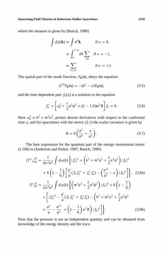
where the measure is given by (Bunch, 1980)∫dµ̃(k) ≡

∫d3k if κ = 0,

≡∫ +∞

0dk∑l ,m

if κ = −1,

≡∑k,l ,m

if κ = +1.

The spatial part of the mode function,Yk(x), obeys the equation

1(3)Yk(x) = −(k2− κ)Yk(x), (3.5)

and the time dependent partfk(η) is a solution to the equation

f ′′k +[ω2

k +λ

2a2φ2+ (ξ − 1/6)a2R

]fk = 0. (3.6)

Hereω2k ≡ k2+m2a2, primes denote derivatives with respect to the conformal

timeη, and for spacetimes with the metric (2.1) the scalar curvature is given by

R= 6

(a′′

a3+ κ

a2

). (3.7)

The bare expression for the quantum part of the energy–momentum tensor(2.10b) is (Anderson and Parker, 1987; Bunch, 1980)

⟨Tη

η

⟩QB =

1

4π2a4

∫dµ(k)

{| f ′k|2+

(k2+m2a2+ λ

2a2φ2

)| fk|2

+ 6

(ξ − 1

6

)[a′

a( fk f ∗′k + f ∗k f ′k)−

(a′2

a2− κ

)| fk|2

]}, (3.8a)

〈T〉QB =1

2π2a4

∫dµ(k)

{(m2a2+ λ

2a2φ2

)| fk|2+ 6

(ξ − 1

6

)×[| f ′k|2−

a′

a( fk f ∗′k + f ∗k f ′k)−

(k2+m2a2+ λ

2a2φ2

+ a′′

a− a′2

a2+(ξ − 1

6

)a2R

)| fk|2

]}. (3.8b)

Note that the pressure is not an independent quantity and can be obtained fromknowledge of the energy density and the trace.

P1: FMN



The equation for the mean field (2.9a) also contains the quantity〈ψ2〉. Itsbare expression can be written in terms of the mode functions as follows

〈ψ2〉B = 1

2π2a2

∫dµ(k)| fk|2. (3.8c)

In these expressions the measure is given by∫dµ(k) ≡

∫ +∞0

dk k2 if κ = 0,−1,

≡+∞∑k=1

k2 if κ = +1.

To determine the adiabatic counterterms needed to renormalize these expec-tation values we solve the mode equation (3.6) using a WKB expansion. To obtainthis expansion we first make the variable transformation

fk = (2Wk)−1/2 exp

[∫ η

dη′Wk(η′)]. (3.9)

Substituting Eq. (3.9) into Eq. (3.6) yields

W2k = ω2

k +λ

2a2φ2+

(ξ − 1

6

)a2R− 1

2

(W′′kWk− 3

2

W′2k

W2k

). (3.10)

This equation is then solved iteratively withωk being of adiabatic order zero andthe next two terms on the right-hand-side being of adiabatic order two.7 Thus tosecond adiabatic order the solution forWk is

Wk = ωk + 1

2ωk

[λ

2a2φ2+

(ξ − 1

6

)a2R− 1

2

(ω′′kωk− 3

2

ω′2kω2

k

)]. (3.11)

To renormalize〈ψ2〉B we use a second order adiabatic expansion for the modes. Afourth-order expansion is necessary to cancel the divergences in〈Tµν〉B (Andersonand Parker, 1987; Bunch, 1980). The renormalization counterterms for these quan-tities are

〈ψ2〉ad = 〈ψ2〉Fad−1

4π2a2

∫dµ(k)

λφ2a2

4ω3k

, (3.12a)

⟨Tη

η

⟩ad =

⟨Tη

η

⟩Fad+

1

4π2a4

∫dµ(k)

{λφ2a2

4ωk− λ

2φ4a4

32ω3k

+ m2λ(φ2a2a′2+ φφ′a3a′)8ω5

k

− 5m4λφ2a4a′2

32ω7k

+ 6

(ξ − 1

6

)×[−λ(φ2a′2+ 2φφ′aa′ + κφ2a2)

8ω3k

+ 3m2λφ2a2a′2

8ω5k

]}, (3.12b)

7 The λ2 a2φ2 term is considered to be of second adiabatic order because only terms with up to two

time derivatives ofφ are needed to cancel divergences in〈Tµν〉B (Paz and Mazzitelli, 1988).

P1: FMN



〈T〉ad = 〈T〉Fad+1

4π2a4

∫dµ(k)

{λφ2a2

2ωk− λφ

2a4(2m2+ λφ2)

8ω3k

+ m2λ

32ω5k

(3λφ4a6+ 4a4φφ′′ + 4a4φ′2+ 8φ2a2a′2+ 8φ2a3a′′

+ 16φφ′a3a′)− 5m4λ

16ω7k

(4φ2a4a′2+ φ2a5a′′ + 2φφ′a5a′)

+ 35m6λa6a′2

32ω9k

+ 6

(ξ − 1

6

)[− λ

4ω3k

(2φφ′aa′ + φ2aa′′ + φφ′′a2

+ φ′2a2+ κφ2a2)+ 3m2λ

8ω5k

(3φ2a2a′2+ 4φφ′a3a′ + 2φ2a3a′′

+ κφ2a4) − 15m4λφ2a4a′2

8ω7k

]}. (3.12c)

The adiabatic counterterms for the free field are (Anderson and Parker, 1987;Bunch, 1980)

〈ψ2〉Fad =1

4π2a2

∫dµ(k)

[1

ωk−(ξ − 1

6

)a2R

2ω3k

+ m2

4ω5k

× (a′2+ aa′′) − 5m4a2a′2

8ω7k

], (3.12d)

⟨Tη

η

⟩Fad =

1

4π2a4

∫dµ(k)

{ωk + m4a2a′2

8ω5k

− m4

32ω7k

(2a2a′a′′′ − a2a′′2

+ 4aa′2a′′ − a′4)+ 7m6a2

16ω9k

(aa′2a′′ + a′4)− 105m8a4a′4

128ω11k

+(ξ − 1

6

)

×[− 3

ωk

(a′2

a2− κ

)− 3m2a′2

ω3k

+ 3m2

4ω5k

(2a′a′′′ − a′′2− a′4

a2

)

− 15m2

8ω7k

(4aa′2a′′ + 3a′4+ κa2a′2)+ 105m6a2a′4

8ω9k

]+(ξ − 1

6

)2

×[− 9

2ω3k

(2a′a′′′

a2− a′′2

a2− 4a′2a′′

a3− 2κa′2

a2+ κ2

)

+ 27m2

ω5k

(a′2a′′

a+ κa′2

)]}, (3.12e)

P1: FMN



〈T〉Fad =1

4π2a4

∫dµ(k)

{m2a2

ωk+ m4a2

4ω5k

(aa′′ + a′2)− 5m6a4a′2

8ω7k

− m4a2

16ω7k

(aa′′′′ + 4a′a′′′ + 3a′′2)+ 7m6a2

32ω9k

(4a2a′a′′′ + 18aa′2a′′

+ 3a2a′′2+ 3a′4)− 231m8a4

32ω11k

(aa′2a′′ + a′4)+ 1155m10a6a′4

128ω13k

+(ξ − 1

6

)[− 6

ωk

(a′′

a− a′2

a2

)− 3m2

ω3k

(2aa′′ − a′2+ κa2)

+ 9m4a2a′2

ω5k

+ 3m2

2ω5k

(aa′′′′ − 2

a′2a′′

a+ a′4

a2

)− 15m4

4ω7k

(4a2a′a′′′

+ 3a2a′′2+ 8aa′2a′′ − a′4+ κa3a′′ + κa2a′2)+ 105m6a2

8ω9k

(8aa′2a′′

+ 5a′4+ κa2a′2)− 945m8a4a′4

8ω11k

]+(ξ − 1

6

)2 [− 9

ω3k

(a′′′′

a− 4a′a′′′

a2

− 3a′′2

a2+ 6a′2a′′

a3− 2κa′′

a+ 2κa′2

a2

)+ 27m2

2ω5k

(4a′a′′′ + 3a′′2

− 6a′2a′′

a+ 4κaa′′ − 2κa′2+ a2κ2

)− 135m4

ω7k

(aa′2a′′ + κa2a′2)

]}.

(3.12f)

Equations (3.12b)–(3.12c) [together with (3.12d)–(3.12f)] give the adiabatic coun-terterms needed to obtain the renormalized values of〈ψ2〉 and〈Tµν〉 for a λφ4-interacting quantum scalar field in a RW spacetime, for the case of a homogeneousmean fieldφ(η).8

4. ANALYTIC APPROXIMATIONS

As it stands the method of adiabatic regularization can be used to computethe quantities〈ψ2〉R and〈Tµν〉R. This then allows one to obtain a self-consistentsolution to the mean field and mode equations (2.9a) and (2.9b) in a backgroundRW spacetime (in the test field approximation) or to these equations plus the semi-classical backreaction equations in a RW spacetime. But before getting involved

8 Mazzitelli and Paz presented these counterterms with the points separated and with the divergencestructure given in the context of dimensional regularization (Paz and Mazzitelli, 1988). Ramsey andHu carried out the adiabatic expansion up to order four forξR = 0 in the context of the leading 1/Nexpansion (Ramsey and Hu, 1997a,b).

P1: FMN



in the backreaction problem (and the difficulties this presents), it would be veryuseful to have a way of estimating how big or small the quantum corrections arebeyond test field approximation. In this section we discuss this issue and presentsuch an approximation.

For a free quantum scalar field in a RW spacetime, Anderson and Eaker haveshown that there is a way of defining a certain approximate energy–momentumtensor that is covariantly conserved (Anderson and Eaker, 2000). In the present pa-per we extend this method to interacting quantum fields and discuss its advantagesand limitations.

The analytic approximations result from a revision of the method of adiabaticregularization that simplifies the calculations in a RW spacetime with compactspatial sections, and in the process yields approximations for the quantities〈ψ2〉Rand〈Tµν〉R. These analytic approximations give information about vacuum polar-ization effects but not particle production, since particle production is a nonlocalphenomenon. However, they also make it possible to solve the mean field, mode,and semiclassical backreaction equations in an approximate manner, which goesbeyond the test field approximation and does not involve a full backreaction cal-culation. This can be useful, for example, if one wishes to determine under whatconditions vacuum polarization effects will be important and what influence theymay have on the mean field and the spacetime geometry. In particular, we believethat these analytic approximations may provide important information for reheat-ing calculations, just before particle production from the inflaton field takes place.The analytic approximations provide a natural way to estimate the change in thevacuum polarization energy of the inflaton field. During the inflationary regimethe mean fieldφ dominates the energy density of the universe. It is reasonable toexpect that when the vacuum polarization energy is of the order of the mean fieldenergy density, the inflaton field will switch from the slow-roll regime to the os-cillatory behavior, that will eventually lead to particle production. In this paper werestrict ourselves to presenting the analytic approximations and our method forobtaining them.

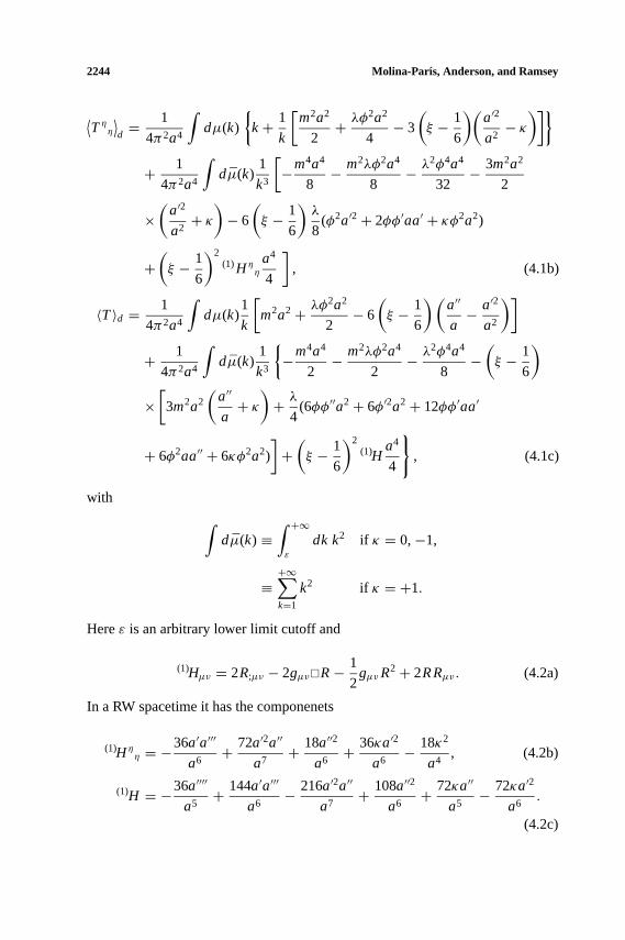
In order to derive the analytic approximation we first improve on the method ofadiabatic regularization by expanding the renormalization counterterms in inversepowers ofk, keeping only terms which are ultraviolet divergent. For the case ofcompact spatial sections (κ = +1) the integral is also changed into a sum. Wecall the resulting expressions〈ψ2〉d and 〈Tµν〉d, respectively. In a general RWspacetime they have the form

〈ψ2〉d = 1

4π2a2

∫dµ(k)

1

k− 1

4π2a2

∫dµ̄(k)

1

k3

×[

m2a2

2+ λφ

2a2

4+(ξ − 1

6

)a2R

2

], (4.1a)

P1: FMN



⟨Tη

η

⟩d= 1

4π2a4

∫dµ(k)

{k+ 1

k

[m2a2

2+ λφ

2a2

4− 3

(ξ − 1

6

)(a′2

a2− κ

)]}+ 1

4π2a4

∫dµ̄(k)

1

k3

[−m4a4

8− m2λφ2a4

8− λ

2φ4a4

32− 3m2a2

2

×(

a′2

a2+ κ

)− 6

(ξ − 1

6

)λ

8(φ2a′2+ 2φφ′aa′ + κφ2a2)

+(ξ − 1

6

)2(1)Hη

η

a4

4

], (4.1b)

〈T〉d = 1

4π2a4

∫dµ(k)

1

k

[m2a2+ λφ

2a2

2− 6

(ξ − 1

6

)(a′′

a− a′2

a2

)]+ 1

4π2a4

∫dµ̄(k)

1

k3

{−m4a4

2− m2λφ2a4

2− λ

2φ4a4

8−(ξ − 1

6

)×[3m2a2

(a′′

a+ κ

)+ λ

4(6φφ′′a2+ 6φ′2a2+ 12φφ′aa′

+ 6φ2aa′′ + 6κφ2a2)

]+(ξ − 1

6

)2(1)H

a4

4

}, (4.1c)

with ∫dµ̄(k) ≡

∫ +∞ε

dk k2 if κ = 0,−1,

≡+∞∑k=1

k2 if κ = +1.

Hereε is an arbitrary lower limit cutoff and

(1)Hµν = 2R;µν − 2gµν¤R− 1

2gµνR2+ 2RRµν. (4.2a)

In a RW spacetime it has the componenets

(1)Hηη = −36a′a′′′

a6+ 72a′2a′′

a7+ 18a′′2

a6+ 36κa′2

a6− 18κ2

a4, (4.2b)

(1)H = −36a′′′′

a5+ 144a′a′′′

a6− 216a′2a′′

a7+ 108a′′2

a6+ 72κa′′

a5− 72κa′2

a6.

(4.2c)

P1: FMN



The renormalized energy–momentum tensor is then computed by subtracting andadding the quantity〈Tµν〉d to Eq. (3.2b), with the result that

〈Tµν〉R ≡ 〈Tµν〉n + 〈Tµν〉an, (4.3a)

〈Tµν〉n ≡ 〈Tµν〉B − 〈Tµν〉d, (4.3b)

〈Tµν〉an ≡ 〈Tµν〉d − 〈Tµν〉ad. (4.3c)

In general〈Tµν〉n must be computed numerically while〈Tµν〉an can always becomputed analytically. The result is

〈ψ2〉an = 〈ψ2〉Fan−λφ2

16π2

{1−

[log

(2ε

aµ

)− κ(κ + 1)

2(logε + γ )

]}, (4.4a)

⟨Tη

η

⟩an= ⟨Tη

η

⟩Fan+

λ

4π2

{−φ

2

48

κ(κ + 1)

2a2− φ

2

16

(m2+ λφ

2

2

)+ φ

2

8

(m2+ λφ

2

4

)[log

(2ε

aµ

)− κ(κ + 1)

2(logε + γ )

]}+ (6ξ − 1)λ

16π2a4

(a2κ

φ2

2+ a′2

φ2

2+ aa′φφ′

)[log

(2ε

aµ

)− κ(κ + 1)

2(logε + γ )

]− λ

96π2a4

(a′2φ2

2+ aa′φφ′

)− (6ξ − 1)λ

16π2a4

(a2κ

φ2

2+ a′2φ2+ aa′φφ′

), (4.4b)

〈T〉an = 〈T〉Fan+λ

4π2

{−φ

2

48

κ(κ + 1)

a2− φ

2

4

(3m2

2+ λφ

2

2

)+ φ

2

4

(2m2+ λφ

2

2

)[log

(2ε

aµ

)− κ(κ + 1)

2(logε + γ )

]}+ (6ξ − 1)λ

16π2a3(aκφ2+ a′′φ2+ 2a′φφ′ + aφ′2+ aφφ′′)

[log

(2ε

aµ

)− κ(κ + 1)

2(logε + γ )

]− λ

96π2a4

(3a4λ

φ4

4+ a2φ′2+ a2φφ′′

+ aa′′φ2+ 2aa′φφ′)− (6ξ − 1)λ

16π2a4

(3a2κ

φ2

2+ a′2

φ2

2+ 4aa′φφ′

+ 2aa′′φ2+ a2φ′2+ a2φφ′′)

, (4.4c)

P1: FMN



with

〈ψ2〉Fan = −a′′

48π2a3+ 1

4π2

{−m2

4− κ(κ + 1)

24a2+ m2

2

[log

(2ε

aµ

)− κ(κ + 1)

2(logε + γ )

]}− (ξ − 1/6)R

8π2

{1−

[log

(2ε

aµ

)− κ(κ + 1)

2(logε + γ )

]}, (4.5a)

⟨Tη

η

⟩Fan =

1

2880π2

[−1

6(1)Hη

η + (3)Hηη − 3κ(κ + 1)

a4

]+ m2

288π2Gη

η

− m2κ(κ − 1)

192π2a2− m4

64π2

[1

2+ 2 log

(µa

2ε

)+ κ(κ + 1)(γ + logε)

]+(ξ − 1

6

)[ (1)Hηη

288π2+ κ(κ − 1)

32π2a4

(1+ a′2

a2

)+ m2

16π2Gη

η

×(

3+ 2 log

(µa

2ε

)+ κ(κ + 1)(γ + logε)

)+ 3κm2

8π2a2

]

+(ξ − 1

6

)2 [ (1)Hηη

32π2

(2+ 2 log

(µa

2ε

)+ κ(κ + 1)(γ + logε)

)− 9

4π2

(a′2a′′

a7+ κa′2

a6

)], (4.5b)

〈T〉Fan =1

2880π2

[−1

6(1)H + (3)H

]+ m2

288π2G− m2κ(κ − 1)

96π2a2

− m4

16π2

[1+ 2 log

(µa

2ε

)+ κ(κ + 1)(γ + logε)

]+(ξ − 1

6

)×[ (1)H

288π2+ κ(κ − 1)

16π2a4

(a′′

a− a′2

a2

)+ m2

16π2G

(3+ 2 log

(µa

2ε

)

+ κ(κ + 1)(γ + logε)

)+ 3κm2

8π2a2− 3m2a′2

8π2a4

]+(ξ − 1

6

)2

×[ (1)H

32π2

(2+ 2 log

(µa

2ε

)+ κ(κ + 1)(γ + logε)

)− 9

8π2

(4a′a′′′

a6− 10a′2a′′

a7+ 3a′′2

a6+ 4κa′′

a5− 6κa′2

a6+ κ

2

a4

)]. (4.5c)

P1: FMN



HereGµν is the Einstein tensor with components

Gηη = −3a′2

a4− 3κ

a2, (4.6a)

G = −6a′′

a3− 6κ

a2= −R, (4.6b)

and(3)Hµν is the tensor

(3)Hµν = RµρRρν − 2

3RRµν − 1

2Rρσ Rρσgµν + 1

4R2gµν , (4.7a)

with components

(3)Hηη = 3a′4

a8+ 6κa′2

a6+ 3κ2

a4, (4.7b)

(3)H = 12a′2a′′

a7− 12a′4

a8+ 12κa′′

a5− 12κa′2

a6. (4.7c)

For a massive fieldµ = m, while for a massless fieldµ is an arbitrary mass scale.However, in the massless case each of the terms in〈Tµν〉an which contains a factorof logµ has as a coefficient a multiple of the tensor(1)Hµν , which comes from anR2 term in the gravitational Lagrangian. Thus, the terms containing logµ simplycorrespond to a finite renormalization of the coefficient of theR2 term in thegravitational action.

Note that ifκ = +1, 〈ψ2〉d and〈Tµν〉d contain a sum overk, while 〈ψ2〉ad

and〈Tµν〉ad contain an integral overk. Thus, either the integral must be convertedto a sum or the sum to an integral. We have converted the sum to an integral usingthe Plana sum formula (Ghika and Visinescu, 1978; Lindelof, 1905; Shenet al.,1985; Whittaker and Watson, 1927). This formula is

+∞∑n=m

f (n) = 1

2f (m)+

∫ +∞m

dx f(x)+ i∫ +∞

0

dt

e2π t − 1[ f (m+ i t )− f (m− i t )].

(4.8)

Because of the way〈Tµν〉d is defined, the third term in the Plana sum formulacan be computed exactly. In the traditional form of adiabatic regularization onewould convert the integral in the adiabatic counterterms to a sum using the Planasum formula and then substitute the result into Eq. (3.2b). However, if this isdone then, for a massive field, it is not possible to compute the third term inthe Plana sum formula analytically. Thus, the computation of the renormalizedenergy–momentum tensor is simplified by our method in theκ = +1 case. Thesame simplification would occur if one was using compact spatial sections forκ = 0 orκ = −1 RW spacetimes.

P1: FMN



5. CONSERVATION OF THE ENERGY–MOMENTUM TENSOR

In this section we show that the renormalized energy–momentum tensor fortheλφ4 theory (at one-loop) in a RW spacetime is covariantly conserved. In a RWspacetime there is only one nontrivial conservation equation which is

Tηη,η + 4a′

aTη

η − a′

aT = 0. (5.1)

We have shown that the energy–momentum tensor for the field can be dividedinto a classical and a quantum part. First consider the classical part which in a RWspacetime has the components (3.3c) and (3.3d). Substituting into Eq. (5.1) andusing (3.3a) we find⟨

Tηη

⟩CR,η +

4a′

a

⟨Tη

η

⟩CR −

a′

a〈T〉CR = −

λ

2φφ′〈ψ2〉R. (5.2)

Thus, the classical energy–momentum tensor is conserved only if there is noquantum correction to the effective mass of the mean field.

The renormalized energy–momentum tensor for the quantum part consistsof the difference between the bare contribution and the adiabatic counterterms.The components of the bare part are given in Eqs. (3.8a) and (3.8b). If they aresubstituted into Eq. (5.1) and the Eq. (3.3b) is used then one finds⟨

Tηη

⟩QB,η +

4a′

a

⟨Tη

η

⟩QB −

a′

a〈T〉QB =

λ

2φφ′〈ψ2〉B. (5.3)

If one substitutes the adiabatic counterterms (3.12b) and (3.12c) into Eq. (5.1) andcompares the result with Eq. (3.2a), one finds⟨

Tηη

⟩ad,η +

4a′

a

⟨Tη

η

⟩ad− a′

a〈T〉ad = λ

2φφ′〈ψ2〉ad. (5.4)

Combining these results and using (3.2a) and (3.2b), one finds that the total renor-malized energy–momentum tensor, classical plus quantum, is conserved. (SeeAppendix A and Appendix B for the details of the proof.)

One further finds that if the analytic approximation is used in place of〈ψ2〉R inthe equation for the mean field and if it is used for the quantum energy–momentumtensor, then the (full) analytically approximated energy–momentum tensor is con-served. This means that one can use the analytic approximation to define a con-sistent set of equations for the mean and the quantum fields, and to be the sourcein the right-hand-side of Einstein’s equation to solve a first approximation to thebackreaction problem.

Thus 〈ψ2〉an and 〈Tµν〉an can be used in place of〈ψ2〉R and 〈Tµν〉R inEqs. (2.9a), (2.10a), and (2.10b) to obtain an analytic approximation for the system.Forκ = 0,−1 RW spacetimes the terms being approximated contain the arbitraryconstantε. This means the approximation is not unique unless the coefficients of

P1: FMN



the logε terms vanish. It is important to note that this is only true when using〈ψ2〉an and〈Tµν〉an as an analytic approximation. Theε dependent terms do notappear in the exact renormalized expressions for these quantities.

From the DeWitt-Schwinger expansion (Christensen, 1976, 1978) it is knownthat for a free quantum field in the large mass limit〈ψ2〉R and〈Tµν〉R have lead-ing order terms proportional to 1/m2. Thus, the analytic approximations for thesequantities are not good approximations in this limit. Previous numerical work(Anderson, 1985, 1986) indicates that the relevant condition is likely to bema¿ 1.The analytically approximated quantities are also local in the sense that they de-pend on the scale factor and its derivatives at a given timeη. Therefore, theycannot accurately describe particle production effects which are inherently nonlo-cal. However, for massless fields they should allow one to estimate how importantvacuum polarization effects are and how they qualitatively modify the evolutionof the system.

6. SUMMARY

We have used adiabatic regularization to renormalize a scalar field theorywith a quartic self-coupling (of the formλφ4) in an arbitrary RW spacetime. Wehave found that the energy–momentum tensor can be naturally split into two parts,a “classical” contribution (which corresponds to the energy–momentum tensorof a classical scalar field with a quartic interaction in a RW spacetime) and a“quantum” piece (which corresponds to the energy–momentum tensor of a freequantum scalar field with the time dependent massm2+ λφ2

2 ). We have displayedthe renormalization counterterms for both the energy–momentum tensor and thecontribution of the quantum fluctuations to the effective mass of the mean field atone-loop order. We have directly checked to see if the energy momentum tensoris covariantly conserved and found that while the entire tensor is conserved, itsclassical and quantum contributions are not separately conserved.

By using a variant on the adiabatic regularization method we have derivedanalytic approximations for the energy–momentum tensor and the contributionof the quantum fluctuations to the effective mass of the mean field. We haveshown that the analytically approximated energy–momentum tensor is covariantlyconserved. Thus the analytic approximations can be used in a self-consistent wayto find approximate solutions to the mean field and backreaction equations. Theapproximations can provide a useful tool for learning about vacuum polarizationeffects for massless fields. However, they are not useful for massive fields in thelarge mass limit. They do not give any significant amount of information aboutparticle production, which is a nonlocal phenomenon.

The approximations could be of use in reheating calculations, in particularthe transition from the slow-roll dynamics of the inflaton field to the oscillatory be-havior around the minimum of the effective potential, (which is believed to produce

P1: FMN



particles of lighter masses), and in the context of relativistic heavy ion collisionas a way of estimating the physical energy density and pressure of the vacuumand thermal excitations. The advantage of this approximation is that one obtainsanalytic expressions for the quantum piece of the energy–momentum tensor, with-out need to solve exactly the mode equation (which is the most difficult part toimplement in numeric computations). In this way, it is relatively easy to study thebackreaction problem of the full system (mean field, quantum fluctuations, andgravitational field).

We believe that this program can be carried forward and improved easily.We plan to extend the present approach and approximations to two-loop order andto the 1/N expansion. We also plan to perform some specific calculations withapplications to reheating and early density perturbations.

APPENDIX A: CONSERVATION OF THE BAREENERGY–MOMENTUM TENSOR

In this Appendix we show that the bare energy–momentum tensor for theλφ4

theory (at one-loop) is covariantly conserved. We start by looking at the equationsof motion

(¤+m2+ ξR)φ + λ

3!φ3+ λ

2φ〈ψ2〉 = 0, (A.1a)

(¤+m2+ ξR)ψ + λ2φ2ψ = 0. (A.1b)

We assume that the mean field is homogeneousφ = φ(η) and write in conformaltime (primes are time derivatives with respect to conformal time)

φ′′ + 2a′

aφ′ + a2

(m2+ ξR+ λ

3!φ2+ λ

2〈ψ2〉

)φ = 0, (A.2a)

ψ ′′ + 2a′

aψ ′ −1(3)ψ + a2

(m2+ ξR+ λ

2φ

)ψ = 0. (A.2b)

The bare energy–momentum tensor is given by

〈Tµv(φ, ψ)〉B = (1− 2ξB)∂µφ∂νφ + (2ξB − 1/2)gµν∂τφ∂τφ − 2ξBφ∇µ∇νφ

+ 2ξBgµνφ¤φ − ξBGµνφ2+ m2

B

2gµνφ

2+ λB

4!gµνφ

4

+ (1− 2ξB)〈∂µψ∂νψ〉 + (2ξB − 1/2)gµν〈∂τψ∂τψ〉− 2ξB〈ψ∇µ∇νψ〉 + 2ξBgµν〈ψ¤ψ〉 − ξBGµν〈ψ2〉

+ m2B

2gµν〈ψ2〉 + λB

4!gµν6φ

2〈ψ2〉, (A.3a)

P1: FMN



with the first two lines corresponding to the classical piece of the energy–momentum tensor and the last two lines to the quantum contribution, that is

〈Tµν(φ, ψ)〉CB def= (1− 2ξB)∂µφ∂νφ + (2ξB − 1/2)gµν∂τφ∂τφ − 2ξBφ∇µ∇νφ

+ 2ξBgµνφ¤φ − ξBGµνφ2+ m2

B

2gµνφ

2+ λB

4!gµνφ

4, (A.3b)

〈Tµν(φ, ψ)〉QB def= (1− 2ξB)〈∂µψ∂νψ〉 + (2ξB − 1/2)gµν〈∂τψ∂τψ〉− 2ξB〈ψ∇µ∇νψ〉 + 2ξBgµν〈ψ¤ψ〉 − ξBGµν〈ψ2〉

+ m2B

2gµν〈ψ2〉 + λB

4gµνφ

2〈ψ2〉. (A.3c)

Theηη component is given by

〈Tηη(φ, ψ)〉B = 1

2φ′φ′ + 6ξB

a′

aφφ′ + 3ξB

(a′2

a2+ κ

)φ2+ a2m2

B

2φ2+ a2λB

4!φ4

+ 1

2〈ψ ′ψ ′〉 − 1

2〈ψ1(3)ψ〉 + 6ξB

a′

a〈ψψ ′〉 + 3ξB

(a′2

a2+ κ

)〈ψ2〉

+ a2m2B

2〈ψ2〉 + a2λB

4φ2〈ψ2〉, (A.4a)

and the trace

〈T(φ, ψ)〉B = (6ξB − 1)1

a2φ′φ′ + 6

a2ξBφφ

′′ + 12

a2ξB

a′

aφφ′

+ ξB Rφ2+ 2m2Bφ

2+ λB

3!φ4+ (6ξB − 1)

1

a2〈ψ ′ψ ′〉

− 1

a2〈ψ1(3)ψ〉 + 6

a2ξB〈ψψ ′′〉 + 12

a2ξB

a′

a〈ψψ ′〉

+ ξB R〈ψ2〉 + 2m2B〈ψ2〉 + λBφ

2〈ψ2〉. (A.4b)

In order to show that the bare energy–momentum tensor is covariantly conserved,we must prove that

∂η⟨Tη

η(φ, ψ)⟩B+ a′

a

[4⟨Tη

η(φ, ψ)⟩B− 〈T(φ, ψ)〉B

] = 0. (A.5)

In order to make the proof a little bit easier, let us introduce the following notation⟨Tη

η(φ, ψ)⟩B

def= 1

a2Kη, and 〈T(φ, ψ)〉B def= 1

a2KT . (A.6)

P1: FMN



The conservation equation now becomes

∂ηKη + a′

a(2Kη −KT ) = 0, (A.7)

with

Kη = 1

2φ′φ′ + 6ξB

a′

aφφ′ + 3ξB

(a′2

a2+ κ

)φ2+ a2m2

B

2φ2+ a2λB

4!φ4

+ 1

2〈ψ ′ψ ′〉 − 1

2

⟨ψ1(3)ψ

⟩+ 6ξBa′

a〈ψψ ′〉 + 3ξB

(a′2

a2+ κ

)〈ψ2〉

+ a2m2B

2〈ψ2〉 + a2λB

4φ2〈ψ2〉, (A.8a)

KT = (6ξB − 1)φ′φ′ + 6ξBφφ′′ + 12ξB

a′

aφφ′ + ξBa2Rφ2+ 2a2m2

Bφ2

+ a2λB

3!φ4+ (6ξB − 1)〈ψ ′ψ ′〉 − ⟨ψ1(3)ψ

⟩+ 6ξB〈ψψ ′′〉

+ 12ξBa′

a〈ψψ ′〉 + ξBa2R〈ψ2〉 + 2a2m2

B〈ψ2〉 + a2λBφ2〈ψ2〉. (A.8b)

In order to present a more explicit proof, we treat the classical and quantum piecesseparately. We start with the classical terms9

∂ηKCη = φ′φ′′ + 6ξ

a′

a(φ′φ′ + φφ′′)+ 6ξ

(a′′

a− a′2

a2

)φφ′

+ 6ξ(κ + a′2

a2

)φφ′ + 6ξ

a′

a

(a′′

a− a′2

a2

)φ2+ aa′m2φ2

+ a2m2φφ′ + aa′λ12

φ4+ a2λ

3!φ3φ′, (A.8c)

2KCη −KC

T = φ′φ′ + 12ξa′

aφφ′ + 6ξ

(a′2

a2+ κ

)φ2

+ a2m2φ2+ a2λ

12φ4+ (1− 6ξ )φ′φ′ − 6ξφφ′′ − 12ξ

a′

aφφ′

− ξBa2Rφ2− 2a2m2Bφ

2− a2λB

3!φ4

= (2− 6ξ )φ′φ′ − 6ξφφ′′ + 6ξ

(a′2

a2− a′′

a

)φ2− a2m2φ2− a2λ

12φ4.

(A.8d)

9 We have dropped the bare subscript from the coupling constantsm, ξ , andλ.

P1: FMN



We can conclude then [by making use of the equation of motion forφ(η), Eq. (A.2a),in the termφφ′′], that

∂ηKCη +

a′

a

(2KC

η −KCT

) = −a2λ

2φφ′〈ψ2〉,

∂η⟨Tη

η

⟩C + a′

a

(4⟨Tη

η

⟩C − 〈T〉C) = −λ2φφ′〈ψ2〉. (A.9)

The proof for the quantum contribution to the energy–momentum tensor goesalong the same lines. By defining10

KQη =

1

2〈ψ ′ψ ′〉 − 1

2

⟨ψ1(3)ψ

⟩+ 6ξBa′

a〈ψψ ′〉 + 3ξB

(a′2

a2+ κ

)〈ψ2〉

+ a2m2B

2〈ψ2〉 + a2λB

4φ2〈ψ2〉, (A.10a)

KQT = (6ξB − 1)〈ψ ′ψ ′〉 − ⟨ψ1(3)ψ

⟩+ 6ξB〈ψψ ′′〉 + 12ξBa′

a〈ψψ ′〉

+ ξBa2R〈ψ2〉 + 2a2m2B〈ψ2〉 + a2λBφ

2〈ψ2〉, (A.10b)

we have then

∂ηKQη = 〈ψ ′ψ ′′〉 −

⟨ψ ′1(3)ψ

⟩+ 6ξa′

a〈ψ ′ψ ′ + ψψ ′′〉

+ 6ξ

(a′′

a− a′2

a2

)〈ψψ ′〉 + 6ξ

(a′2

a2+ κ

)〈ψψ ′〉

+ 6ξa′

a

(a′′

a− a′2

a2

)〈ψψ ′〉 + aa′m2〈ψ2〉 + a2m2〈ψψ ′〉

+ a2λ

2φ2〈ψψ ′〉 + a2λ

2φφ′〈ψ2〉 + aa′λ

2φ2〈ψ2〉, (A.10c)

2KQη −KQ

T = (2− 6ξ )〈ψ ′ψ ′〉 − 6ξ〈ψψ ′′〉 + 6ξ

(a′2

a2− a′′

a

)〈ψ2〉

− a2m2〈ψ2〉 − a2λ

2φ2〈ψ2〉. (A.10d)

10As the quantum contribution to the full energy–momentum tensor is already one-loop, we canconsider all the parameters,m, ξ , andλ to be the renormalized ones.

P1: FMN



We can conclude then [by making use of the equation of motion forψ , Eq. (A.2b),in the termψψ ′′], that

∂ηKQn +

a′

a

(2KQ

η −KQT

) = a2λ

2φφ′〈ψ2〉,

∂η⟨Tη

η

⟩Q + a′

a

(4⟨Tη

η

⟩Q − 〈T〉Q) = λ

2φφ′〈ψ2〉. (A.11)

If we consider the sum of both contributions [Eqs. (A.9) and (A.11)], it is easy tosee that

∂η⟨Tη

η(φ, ψ)⟩B+ a′

a

[4⟨Tη

η(φ, ψ)⟩B− 〈T(φ, ψ)〉B

] = 0. (A.12)

One important point that needs to be mentioned, although it should be clear fromthe previous proofs, is that neither the classical, nor the quantum piece of theenergy–momentum tensor is conserved by itself, as has been shown above.

APPENDIX B: CONSERVATION OF THE RENORMALIZEDENERGY–MOMENTUM TENSOR

The first question that needs to be addressed is how to define the renormalizedenergy–momentum tensor. In order to answer this question, we point out at thisstage that the divergences of〈ψ2〉B can all be absorbed in the bare couplingconstantsm2

B, ξB, andλB, as we have shown in a previous Section, after defining

〈ψ2〉R = 〈ψ2〉B − 〈ψ2〉ad. (B.1)

This scheme defines the renormalized parametersm2R, ξR, andλR. We can then

write the renormalized equation of motion for the mean field in terms of theseparameters to obtain

φ′′ = −2a′

aφ′ − a2

(m2

R+ ξRR+ λR

2φ2

)φ − λR

2φ〈ψ2〉R, (B.2)

with 〈ψ2〉R defined by the previous equation.The bare classical energy–momentum tensor has ultraviolet divergences be-

cause it is given in terms of the bare parameters that are divergent themselves. Therenormalized classical energy–momentum tensor is given by

〈Tµν(φ, ψ)〉CR def= (1− 2ξR)∂µφ∂νφ + (2ξR− 1/2)gµν∂τφ∂τφ − 2ξRφ∇µ∇νφ

+ 2ξRgµνφ¤φ − ξRGµνφ2+ m2

R

2gµνφ

2+ λR

4!gµνφ

4, (B.3)

which is a finite quantity. It is easy to show that this tensor is not covariantlyconserved, in fact

∂η⟨Tη

η(φ, ψ)⟩CR +

a′

a

[4⟨Tη

η(φ, ψ)⟩CR − 〈T(φ, ψ)〉CR

] = −λR

2φφ′〈ψ2〉R. (B.4)

P1: FMN



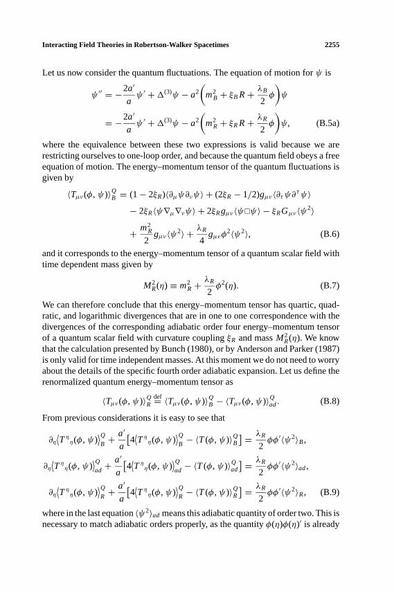
Let us now consider the quantum fluctuations. The equation of motion forψ is

ψ ′′ = −2a′

aψ ′ +1(3)ψ − a2

(m2

B + ξB R+ λB

2φ

)ψ

= −2a′

aψ ′ +1(3)ψ − a2

(m2

R+ ξRR+ λR

2φ

)ψ, (B.5a)

where the equivalence between these two expressions is valid because we arerestricting ourselves to one-loop order, and because the quantum field obeys a freeequation of motion. The energy–momentum tensor of the quantum fluctuations isgiven by

〈Tµν(φ, ψ)〉QB = (1− 2ξR)〈∂µψ∂νψ〉 + (2ξR− 1/2)gµν〈∂τψ∂τψ〉− 2ξR〈ψ∇µ∇νψ〉 + 2ξRgµν〈ψ¤ψ〉 − ξRGµν〈ψ2〉

+ m2R

2gµν〈ψ2〉 + λR

4gµνφ

2〈ψ2〉, (B.6)

and it corresponds to the energy–momentum tensor of a quantum scalar field withtime dependent mass given by

M2R(η) ≡ m2

R+λR

2φ2(η). (B.7)

We can therefore conclude that this energy–momentum tensor has quartic, quad-ratic, and logarithmic divergences that are in one to one correspondence with thedivergences of the corresponding adiabatic order four energy–momentum tensorof a quantum scalar field with curvature couplingξR and massM2

R(η). We knowthat the calculation presented by Bunch (1980), or by Anderson and Parker (1987)is only valid for time independent masses. At this moment we do not need to worryabout the details of the specific fourth order adiabatic expansion. Let us define therenormalized quantum energy–momentum tensor as

〈Tµν(φ, ψ)〉QR def= 〈Tµν(φ, ψ)〉QB − 〈Tµν(φ, ψ)〉Qad. (B.8)

From previous considerations it is easy to see that

∂η⟨Tη

η(φ, ψ)⟩QB +

a′

a

[4⟨Tη

η(φ, ψ)⟩QB − 〈T(φ, ψ)〉QB

] = λR

2φφ′〈ψ2〉B,

∂η⟨Tη

η(φ, ψ)⟩Qad +

a′

a

[4⟨Tη

η(φ, ψ)⟩Qad − 〈T(φ, ψ)〉Qad

] = λR

2φφ′〈ψ2〉ad,

∂η⟨Tη

η(φ, ψ)⟩QR +

a′

a

[4⟨Tη

η(φ, ψ)⟩QR − 〈T(φ, ψ)〉QR

] = λR

2φφ′〈ψ2〉R, (B.9)

where in the last equation〈ψ2〉ad means this adiabatic quantity of order two. This isnecessary to match adiabatic orders properly, as the quantityφ(η)φ(η)′ is already

P1: FMN



of adiabatic order three. The presence of the adiabatic order four term on theright-hand-side would make it impossible to cancel out the adiabatic order seventerms that this procedure will generate (as the left-hand-side is of adiabatic orderfive). In fact, it is not very hard to show that indeed, this last equation is not onlyapproximately valid, but that it is an identity.

It is now time to put all these pieces together and define the renormalizedenergy–momentum tensor for the full system (mean field and fluctuations). Wedefine

〈Tµν(φ, ψ)〉R = 〈Tµν(φ, ψ)〉CR + 〈Tµν(φ, ψ)〉QR= 〈Tµν(φ, ψ)〉CR + 〈Tµν(φ, ψ)〉QB − 〈Tµν(φ, ψ)〉Qad. (B.10)

The important question that remains to be answered at this stage is the following: is〈Tµν(φ, ψ)〉R so defined a covariantly conserved energy–momentum tensor? Theanswer is given by the following identities

∂η⟨Tη

η(φ, ψ)⟩CR +

a′

a

[4⟨Tη

η(φ, ψ)⟩CR − 〈T(φ, ψ)〉CR

] = −λR

2φφ′〈ψ2〉R,

∂η⟨Tη

η(φ, ψ)⟩QB +

a′

a

[4⟨Tη

η(φ, ψ)⟩QB − 〈T(φ, ψ)〉QB

] = λR

2φφ′〈ψ2〉B,

∂η⟨Tη

η(φ, ψ)⟩Qad +

a′

a

[4⟨Tη

η(φ, ψ)⟩Qad − 〈T(φ, ψ)〉Qad

] = λR

2φφ′〈ψ2〉ad. (B.11)

We conclude therefore that

∂η⟨Tη

η(φ, ψ)⟩R+ a′

a

[4⟨Tη

η(φ, ψ)⟩R− 〈T(φ, ψ)〉R

]= −λR

2φφ′〈ψ2〉R+ λR

2φφ′〈ψ2〉B − λR

2φφ′〈ψ2〉ad

= λR

2φφ′[〈ψ2〉B − 〈ψ2〉R− 〈ψ2〉ad] = 0, (B.12)

where the last identity follows from the definition of〈ψ2〉R.

ACKNOWLEDGMENTS

The authors wish to express their gratitude to Salman Habib and Emil Mottolafor their incisive comments on the manuscript and endless hours of fruitful dis-cussion. C. M.-P. and P. R. A. thank the organizers of Peyresq 5, especiallyProfs. Edgard Gunzig and Enric Verdaguer for their kind invitation and hospitality.Part of this work was done while P. R. A. was visiting at Montana State University.He would like to thank W. Hiscock and the entire Department of Physics there fortheir hospitality. This work was supported in part by grant number Phy-9800971

P1: FMN



from the National Science Foundation. C. M.-P. was partially supported by theDepartment of Energy under contract W-7405-ENG-36.

REFERENCES

Anderson, P. R. (1985).Physical Review D32, 1302.Anderson, P. R. (1986).Physical Review D33, 1567.Anderson, P. R. and Eaker, W. (2000).Physical Review D61, 024003.Anderson, P. R. and Parker, L. (1987).Physical Review D36, 2963.Birrell, N. D. (1978).Proceedings of the Royal Society of London B361, 513.Birrell, N. D. (1980).Journal of Physics A: Mathematical and General13, 569.Birrell, N. D. and Davies, P. C. W. (1982).Quantum Fields in Curved Space, Cambridge University

Press, England, and references contained therein.Birrell, N. D. and Ford, L. H. (1979).Annals of Physics (New York)122, 1.Birrell, N. D. and Ford, L. H. (1980).Physical Review D22, 330.Boyanovsky, D., Cormier, D., de Vega, H. J., Holman, R., Singh, A., and Srednicki, M. (n.d.). hep-

ph/9609527.Boyanovsky, D., de Vega, H. J., Holman, R., Lee, D.-S., and Singh, A. (1995).Physical Review D52,

6805.Boyanovsky, D., Holman, R., and Prem Kumar, S. (1997).Physical Review D56, 1958.Bunch, T. S. (1980).Journal of Physics A: Mathematical and General13, 1297.Bunch, T. S. and Panangaden, P. (1980).Journal of Physics A: Mathematical and General13, 919.Bunch, T. S., Panangaden, P., and Parker, L. (1980).Journal of Physics A: Mathematical and General

13, 901.Bunch, T. S. and Parker, L. (1980).Physical Review D20, 2499.Christensen, S. M. (1976).Physical Review D14, 2490.Christensen, S. M. (1978).Physical Review D17, 946.Cognola, G. (1994).Physical Review D50, 909.Collins, J. C. (1974).Physical Review D10, 1213.Cooper, F., Kluger, Y., Mottola, E., and Paz, J. P. (1995).Physical Review D51, 2377.Drummond, I. T. (1975).Nuclear Physics B94, 115.Ford, L. H. and Toms, D. J. (1982).Physical Review D25, 1510.Fulling, S. A. and Parker, L. (1974).Annals of Physics(New York) 87, 176.Fulling, S. A., Parker, L., and Hu, B. L. (1974).Physical Review D10, 3905.Ghika, G. and Visinescu, M. (1978).Nuovo Cimento46A, 25.Hu, B. L. (1983).Physics Letters B123, 189, and references contained therein.Jackiw, R. and Kerman, A. (1979).Physics Letters A71, 158.Lampert, M. A., Daswon, J. F., and Cooper, F. (1996).Physical Review D54, 2213, and references

contained therein.Lampert, M. A. and Molina-Par´ıs, C. (1998).Physical Review D57, 83.Lindelof, E. (1905).Le calcul des Residus, Gautier-Villars, Paris.Mazzitelli, F. D. and Paz, J. P. (1989).Physical Review D39, 2234.Mazzitelli, F. D., Paz, J. P., and Hasi, C. El (1989).Physical Review D40, 995.Molina-Par´ıs, C., Anderson, R., and Ramsey, S. A. (2000).Physical Review D61, 127501.Parker, L. (1966). PhD Thesis, Harvard University, Xerox University Microfilms, Ann Arbor, Michigan,

No. 73-31244 and App. CI., pp. 140–171.Parker, L. and Fulling, S. A. (1974).Physical Review D9, 341.Paz, J. P. and Mazzitelli, F. D. (1988).Physical Review D37, 2170.Ramsey, S. A. and Hu, B. L. (1997a).Physical Review D56, 661.

P1: FMN



Ramsey, S. A. and Hu, B. L. (1997b).Physical Review D56, 678.Ringwald, A. (1987).Annals of Physics(New York) 177, 129,Physical Review D36 (1987), 2598.Shen, T. C., Hu, B. L., and O’Connor, D. J. (1985).Physical Review D31, 2401.Stevenson, P. (1985).Physical Review D32, 1389.Suen, W. M. and Anderson, P. R. (1987).Physical Review D35, 2940.Whittaker, E. T. and Watson, G. N. (1927).A Course of Modern Analysis, Cambridge University Press,

London, Exercise 7, p. 145.

interacting field theories in robertson-walker … paz and mazzitelli (1988). they displayed the...

Documents