interaction of a boundary layer with a turbulent wake - nasa · interaction of a boundary layer...

Interaction of a boundary layer with a turbulent wake

Ugo Piomelli Department of Mechanical Engineering

University of Maryland College Park, MD 20742

Final Report for Grant NAG1 2285 monitored by Dr. M. M. Choudhari

The objective of this grant was to study the transition mechanisms on a flat-plate boundary

layer interacting with the wake of a bluff body. This is a simplified configuration, sketched in

Fig. 1, designed to exemplify the phenomena that occur in multi-element airfoils, in which the

wake of an upstream element impinges on a downstream one. Some experimental data is

available for this configuration [l--31 at various Reynolds numbers.

2

Figure I Sketch of the geometric configuration.

50

The first task carried out was the implementation and validation of the immersed-boundary

method [4, 51. This was achieved by performing calculations of the flow over a cylinder at low

and moderate Reynolds numbers. The low-Reynolds number results are discussed in Ref. 6,

https://ntrs.nasa.gov/search.jsp?R=20040110958 2018-07-16T10:20:14+00:00Z

which is enclosed as Appendix A. The high-Reynolds number results are presented in a paper in

preparation for the Journal of Fluid Mexhanics.

We performed calculations of the wakehoundary-layer interaction at two Reynolds numbers,

Re=385 and 1155. The first case is discussed in Ref. 6, and a comparison of the two calculations

is reported in Ref. 7. The simulations indicate that at the lower Reynolds number the boundary

layer is buffeted by the unsteady Karman vortex street shed by the cylinder. This is shown in

Fig. 2: long streaky structures appear in the boundary layer in correspondence of the three-

dimensionalities in the rollers. The fluctuations, however, cannot be self-sustained due to the

low Reynolds-number, and the flow does not reach a turbulent state within the computational

domain. In contrast, in the higher Reynolds-number case, boundary-layer fluctuations persist

after the wake has decayed (due, in part, to the higher values of the local Reynolds number Re

achieved in this case); some evidence could be observed that a self-sustaining turbulence

generation cycle was beginning to be established.

50

0.2

0

0.2

4

0 xz-plme

2 0 Figure 2 Instantaneous flow field for the Re=385 calculation. Iso-surfaces of pressure and streamwise velocity fluctuations.

A third simulation was subsequently carried out at a higher Reynolds number, Re=3900. This

calculation gave results similar to those of the Re=l155 case. Turbulence was established at

fairly low Reynolds number, as a consequence of the high level of the free-stream perturbation.

Figure 3 shos an instantaneous flow visualization for that case.

A detailed examination of flow statistics in the transitional and turbulent regions, including

the evolution of the turbulent kinetic energy (TKE) budget and frequency spectra showed the

formation and evolution of “turbulent spots”‘ characteristic of the bypass transition mechanism.

It was also observed that the turbulent eddies achieved an equilibrium, fully developed turbulent

states first, as evidenced by the early agreement achieved by the terms in the TKE budget with

those observed in turbulent flows (Figs. 4 and 5). Once a turbulent Reynolds stress profile had

been established, the velocity profile began to resemble a turbulent one, first in the inner region

and later in the outer region of the wall layer. An extensive comparison of the three cases,

including budgets, mean velocity and Reynolds stress profiles and flow visualization, is in Ref.

8.

I O

5

Figure 3 Instantaneous floni fie field for the Re=3900 calculation. Iso-su$aces of pressure and streamwise velocity fluctuations.

Copies of Refs. 6 and 7, which discuss the results obtrained, are enclosed.

References

Underlined articles acknowledge NASA support.

1. Kyriakides NK, Kastrinakis EG, Nychas SG, Goulas, A 1996. Proc. Znst. Mech. Eng 21, 167.

2. Kyriakides NK, Kastrinakis EG, Nychas SG, Goulas, A 1999. AZAA J. 37, 1 197.

3. Kyriakides NK. Kastrinakis EG, Nychas SG, Goulas, A 1999. Eur J. Mech. B-Fluid 18,

1049.

4. Fadlun EA, Verzicco R, Orlandi P, Mohd-Yusof J 2000. J. Comput. Phys. 161,35.

5 . Verzicco R, Mohd-Yusof J, Orlandi P, Haworth, D 2000. AZAA J. 38, 427.

Lines -- LES. Symbols -- Moser et a/. (1 999)

0.3 I 1

Rex=l 7325 ---i +++ 0.2 + + _

-0.2y 1 -0.2y 1 0 20 my+ 6o 80 100 80 100

40 Y + 6o 0 20

V.“

0.2

0.1

0

-0.1

-0.2

V.”

x/D=l50 Rex=l 73250 Re8=459

0 20 My+ 6o 80 100

Figure 4 Turbulent kinetic energy budgets, Re=lI55.

80 100 40 Y + 6o

0 20

6 . Piomelli U. Balaras E 2001 In DNSLES Progress and Challenaes. eds. C. Liu. L. Sake11 and

T. Beutner, (Grevden Press. Columbus), ~ p . 105-1 16.

7. Piomelli U. Choudhari MM. Ovchinnikov V. Balaras E 2003 AZAA Pauer 2003-0975.

8. Ovchinnikov V. Piomelli U. Choudhari MM 2004 To be submitted to J. Fluid Mech.

Lines -- LES. Symbols -- Moser et a/. (1 999)

80 100 40Y+ 6o 80 100 0 20 0 20 4oy+ 6o

0 20 My+8Q 80 100

Figure 5 Turbulent kinetic energy budgets, Re=3900.

0.3 I 1 . _

0.2

0.1

0

-0.1

-0.2r 1 1 i

80 100 0 20 4oy+ *

NUMERICAL SIMULATIONS USING THE: IMMERSED BOUNDARY TECHNiQUE

UGO PIOMELLI AND ELIAS BXLAR+U Department of Mechanical Engineering University of Margland College Park, iZID 2074.2 - USA

Abstract. The immersed-boundary method can be used to simulate flows around complex geometries within a Cartesian grid. This method has been used quite extensively in low Reynoids-number Gows, a d is now being applied to turbulent flows more frequently. The technique will be discussed, and three applications of the method will be presented, with increasing complexity, to illustrate the potential and !islitations of the method, and some of the directions for future work.

1. Introduction

The increase in computer speed achieved over the last few years has made computational fluid dynamics increasingly useful and widespread as a tool to analyze and design flow configuration. Complex geometries, however, present an obstacle even to present-day computers, since the use of body- fitted meshes (structured or unstructured) significantly increases the cost of a calculation in terms of both computational speed and memory require- ments.

An alternative method that may be cost-eEcient in many situations is the "immersed-boundary" method. This technique is based on the introduction or' body forces distributed throughout the flow that mimic the effect that a solid body would have on the h i d . This approach allows the use of codes'in Cartesian coordinates, which present iig3ificant advantages, in terms of speed, xciiracy and !h::ibility. over rodw khat employ bodv fitted grids.

This idea has been widely used in hzmo-dynamics and bio-fluids engineering: two- and three-dimensional calculations of the Bow in the heart

2 C‘GO TIOMELLI XXD ELLIS BALARXS

were reported by Peskin [13, 141 and McQueen and Peskin [8, 91. In these calculations the motion of the boundary was determined by the fluid it- se!f, so that the boundary had to be modeled as a set of elements linked by springs. In cases in which the boundary motion is known a priori, the problem can be significantly simplified.

Goldstein e t al. [4] proposed a feedback forcing mechanism that forces the fluid velocity ui to approach the velocity of the solid boundary. V,, on the boundary itself. Consider the incompressible Navier-Stokes equations:

Goldstein et ai. [4] assigned a force field

t fi(xcs,i, t ) = af 1 [ui(xs , i , t ) - ~ ( x s , i , t ) ] dt‘ + pf [ui(xs,ir t ) - v i ( x s , i , t ) ] 7

0 (3)

where a f and Pf are two negative constants, and xs,i are the coordinates of the solid surface. The net effect of this force is to tend to annihilate the velocity difference ui - V,. The flow, in fact, responds to the forcing as a damped oscillator (see [4] and [3] for a n in-depth discussion of this issue); the frequency of the oscillator is x Iaf/’/’, whereas its damping coefficient is c( jlf/1a11/2. This implies that, in order to enforce the nc-slip condition effectively, af and j3f must have large magnitudes (larger than the highest frequency in the flow), which make the equations stiff. If the forcing is advanced in time explicitly, in fact, the maximum allowable CFL is o ( ~ O - ~ ) ; even implicit methods only allow the use of CFL numbers of 0.1 or less. This constraint makes this method impractical for the calculation of unsteady (in particular, turbulent) flows.

Recently, hlohd-Yusof [ll] proposed the “direct forcing met hod,” which assigns a force field given by

(where the dependence on x,,; and t has been omitted). This forcing im- poses directly the desired velocity on the immersed boundary, and has the advantage (over the feedback forcing method) that it does not require significant reductions io the allowable time-step. It w3s exteEsively tested in a staggered finite-difFerence code by Fadlun e t al. [3]! xho derived an interpolation scheme to be used when the boundary does not coincide with a grid

NUMERICAL SLMULATIONS USING THE IMMERSED BOUZIDARY TECHNIQZUB

............ .......

.............. ,," the ..................... i ....... 1 .

................................................................................................

Figure 1. Interpolation mechod used to apply the forcing.

line. Verzicco et al. [15] applied this method to the large-eddy simulation of high Reynolds number turbulent flows by calculating the flow inside an IC engine.

In the present paper additional applications of this method will be presented, and the potential and limitations of the technique, as well as issues that reqfiire further studyi will he disriissed. After a brief review of the governing equations and of the numerical scheme used, three test cases will be shown: a low Reynolds-number flow over a cylinder in the presence of a moving surface (TVannier [16] flow), the flow over a circular cylinder at low Reynolds number, and the bypass transition on a flat plate caused by the interaction between the boundary layer and the wake of a circular cylinder.

2. Problem formulation

Governing the flow are the incompressible Navier-Stokes equations (1 2) . The flow solver is a standard 2nd-order accurate method on a staggered mesh [I]. The fractional time-step method [2, 61 is used and a 2nd-order accurate Adams-Bashforth method is employed fur the time advancement. A non-reflecting boundary condition [12] is used at the outflow, and periodic boundary conditions in the spanwise direction. The inflow and free-stream conditions depended on the case studied.

The direct forcing (4) was used. Since the immersed body does not follow a grid line the interpolation method proposed by Fadlun e t al. [3] is used. The forcing is imposed not at the surface itself, but at the &st point outside it (see Fig. 1) and the soiid body velocity in (4) is replaced with the velocity obtained by a linear interpolation between the computed fluid velocity outside the body, ut , and the desired body velocity V,. This method has several advantages: first. it has been shown to be fully second- order accurate in time [3]; therefore, it is consistent with the sccmd-order differencing scheme used by the solver; secondly, since it assumes that the velocity profile is linear near the body, it implies homogeneous Neumann

4 UGO PIOMELLI AND ELiAS BALAiLiS

1

. *

3

a - I /

- 2 0

$ -10

Figure 2. puted streamlines; (b) LI and LZ norms of the error, E , for u and N is the total number of grid points.

Wannier flow test case (Wannier 1950). (a) Computational domain and com- velocity components.

boundary conditions for the pressure (see the Appendix in [3] for a full discussion of this issue). This last feature is very important in the hamework of fractional time-step methods, since it implies that the corrector step does not result in a modification of the body velocity imposed through the forcing in the Helmholtz step. On the other hand, the assumption that the velocity profile is linear over the first two layers of cells outside the immersed body requires the use of a very fine mesh in the vicinity of the body.

3. Results and discussion

3.1. WANNIER FLOW

X straightforward way to verify the accuracy of the proposed methodology is to compute a flow containing a curved immersed boundary for which an analytical solution exists. The case considered here is the Stokes flow around a cylinder in the vicinity of a moving wall (see Fig. 2). An analytical solution for this case was derived by Wannier [16]. The streamlines for this flow are shown in Fig. 2a. Three computations on gradually finer uniform grids (32 x 32, 64 x 64, and 128 x 128) were conducted. The L1 and L? norms of the error (the difference between the computed and analytical -iolution) are shown in Fig. 2b as a function of the total number of points N . The error decreases with a -2 slope indicating that the proposed methodology is second order accurate.

3.2. FLOW OVER .4 CIRCIJLAR CYLINDER

The next test case examined is the flow over a circular cylinder at Reo = UmD/v = 300 (where D is the cylinder diameter and U, the free-stream

Lu

i 2 5 -

rHE IMMERSED BO CND-ARY TECHYIQUB

Figure 3. (c) (u'u'), (d) (dw'). Reference data from Ref. [lo].

Flow over a circular cylinder, Reo = 300. VeIocity statistics. (a) C', (b) W ,

velocity). Two calculations will be compared: a 2D one that used 400x200 points in the xz-plane, and a 3D one, with the same mesh in the xz-plane, and 48 points in y. The computational Jomain was 60 ;< 2~ x 30. a d the cylinder center was at x, = 10, z , = 15 (all lengths are made dimensionless by D , all velocities by V,). The grid was stretched both in the 2- and z-directions; the last 116 of the domain (which required only 10 grid points in x) formed a sponge region, used to minimize the upstream propagation of disturbances due to the convective outflow conditions. X uniform velocity profile was imposed at the inlet, and slip-wall conditions were applied a t z = 0 and z = 30.

'The velocity statistics are shown in Fig. 3 . Here and in the following the angle brackets denote averaging in time and in the spanwise direction. The 3D calculation is in very good agreement with the reference data by Mittal and Balachandar [lo]. At this Reynolds number, three-dimensionahty is observed in the wake, which is evidenced in the visualization in Fig. 4, which shows iso-surfaces of the second invariant of the velocity-gradient tenssor,

6

0

-4

-?I

2

5

‘0 i

A 4 ’ 5

6

Figure 4. Flow over a circular cylinder, Reo = 300. Isosurfxes of Q = 3.5.

(where nzJ is the anti-symmetric part of the velocity gradient tensor). The condition Q > 0 identifies effectively the regions of coherent vorticity 15:.

Figure 4 shows the formation of an instability on the initially 2D rollers, and the presence of quasi-streamwise rib vortices joining the rollers. The magnitude of the spaxvise Xeynolds stresses (v’v’). in this calcdaciox however. remained significanti.7 smaller than the other two normal components. -xSich ailowed the 2D calculation to give reasonable results.

The ezects of the grid resolution near the obstacle are shown in 9ig. 5 . The cell Reynolds number is defined as

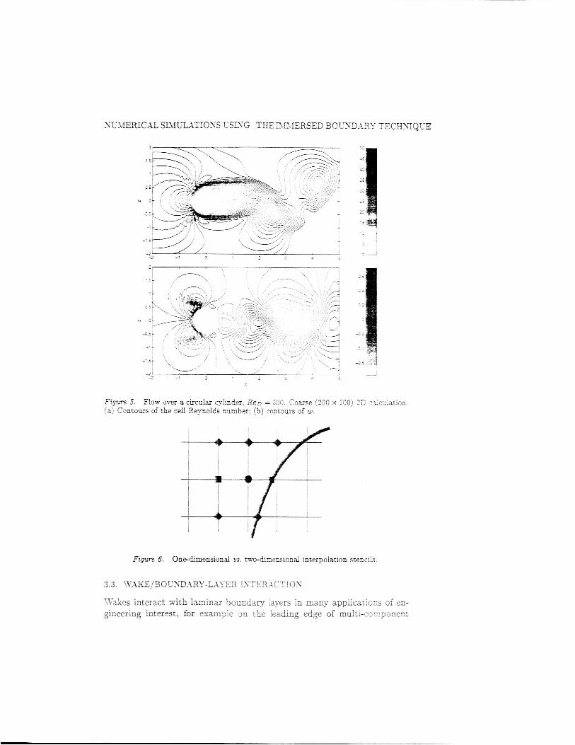
where 1: zxd w are :he illjta-taneous velocities, m d 3.: and 1z ->? 0- +d - spacings. If the inesh is insufficiently fine (Re, > 30), scme csc:;iations can be observed that initiate along lines a t 145’ on the cylincer ,they are especially visible in the w contours, Fig. 5b). Refining the grid. thus reducing Re, reduces the size of this oscillation (Figs. ?a m d 5’. Two- dimensional interpolatioll schemes tha: use bcrh :Le pcizts ixdicrt-d by the diamonds m d those indicated by squarps :n 11%. 6 to ,?e:er=lice V, have also WE fousd (VZ~~CCO, pri:-nte c ~ ~ ~ , l n i c c ~ i i 3 n . 2CO: to reduce the amplitude of these oscillations.

- . 1.

-2 3 *

Figure 5. (a) Contours of the cell Reynolds number; (b) contoun of w.

Flow over a circular cylinder, ReD = 200. Coarse (200 x 100) 7E c&x!ation.

Figure 6. Onedimensional vs. two-dimensional interpolation sxencik

3.3. T~~~XE/E3CUNDIR~-L- IVER 5TTERSCTIC)N

TtVakes interact with laminar boundary !ayFrs in many applicz~ions of eo- gineering interest, for examp!e 3n the !eading edge of multi-com?onent

Figure 7. (a) Contours of the cell Reynolds number; (b) contours of w .

F!ow over a circular cylinder, ReD = 300. Fine (400 x 208) 2D d c n h t i o n .

airfoils, or inside turbemachinery. The interaction of the turbulent eddies ?resent in the wake with the boundary layer itself -hen becomes a primary drjv-r of the transition process ia :he boiindary h y z itself. anld may lead to transition to turbulence at faair!y low Eleynolds numbers.

* . .++cherl :.I r:-r 2

X circular cyiinder, with its axis ncrmal to the stream is placed above a T5e ssdguration e x m i n e d la the pr-sent 3 : ~ ; ; - As :A _. -_& _- - -0. _.

NT;MERICXL SIMULATIONS USCU’G THE MMERSED BOUSDXRY TECHSIQUB

0at plate. The cylinder center is at xc = 10, sc = 3.2, immediateiy above the leading-edge of the plate, which was also at x, = 10. -4s in the previous case, distances +re normalized by D, velocities by U,. The computational domain was 60 x 2 7 x 20. As for the cylinder calculation. the =rid was stretched both in the x- and z-directions and a sponge region was used. The Reynolds number based on cylinder diameter was 385. Thc configuration corresponds to Case 1 in the experimental paper by Kyr:&mies e t al. [7], who observed significant velocicy fluctuations in the boundar:I layer, starting from a point approximately six diameters downstream of :he cylinder. These %uctuations are generated by the large-scale convective motion of the vortices, and do not die down after the wake has weakened, but develop into a turbulent boundary layer despite the fact that the Reynolds number is very low.

The distribution of the streamwise Reynolds stress, (u‘u‘). as a, function of x is shown in Fig. 9. X sudden increase of (u‘u‘) can be observed to begin at x = 8, indicating the beginning of transition. This result is consistent with the observations of Kyriakides et al. [7]> who defined the onset of transition as “the z-location where the velocity signal at the same height above the plate loses its sinusoidal character”, and found that transition occurs at x = 7.4.

The velocity profiles, shown in Fig. 10a at several locations. initially resemble a Blasius profile merging into a wake near the cylinder. As the wake widens and interacts with the boundary layer, a logarithmic layer begins to establish itself, indicative of transition towards turbulent flow. This transitional behavior is also observed in the trace of the Reynolds stress tensor, q2 (equal to twice the turbulent kinetic energy). which in the latter sections establishes a turbulent-like distribution. with a peak of magnitude 7 - 87,,, a t zf 21 10 - 12. It should be noted that this quasi- turbulent state is achieved at very low Reynolds number: the boundary-

t 50 02

o o i t 1

O I /

i b

Figure 9. \Vake/boundary-layer interaction. (u’u’) distribution at i = 0.13.

10 UGO PIOMELLI AND ELMS BALARAS

-5' ' " " " " """ J 1 O P lo-' 10' * 10' 1 o2 1 o1

'0 1 2 3 4 5 6 7 8 9 1 0 1 1 1 2 1 3 V2ITw

4

Figure 10. profile; bottom: q2 = (&A;).

Wake/boundary-layer interaction. Turbulent statistics. Top: mean velocity

layer thickness b (defined a s the distance above the plate at which the first maximum of the velocity profile occurs) is approximately 50-70 wall units.

A visualization of the flow is shown in Fig. 11. The structure of the cylinder wake is similar to that highlighted in Fig. 4, with strong spanwise rollers that exhibit 3D instabilities and eventually break up, and smaller quasi-streamwise vortices in the braid region. The contours of streamwise velocity fluctuation u' on a plane parailel to the wall show significant levels of fluctuations, especially near kinks in the rollers belonging to the lower row. Quasi-streamwise streaks are formed around 2 = 15, whose spacing is approximately 100 wall units.

4. Conclusions

The immersed-boundary techniqiic? has been presented and discussed. 11- iustrative resuits from three simuiacions indicate the potential of this technique, which allows the calculation of flows around ccrcplex geometries without requiring a body-fitted grid.

NI;MERIC.%L SI1cIUL.ATIOYS U S B G THE DISIERSED BOCXD.-IRI- TECHXIQUE

25

4

h 2 n u

6 o 5

Y 2 0 0

" 3 3 10 15 20 25

.r " 7 - Flow _ _

Figure 21. in the z = 0 18 plme Top: perspectwe xew; bottom. mew from above

',Vake/Soundary-iayer anteraction. Isosurfaces or' 2 = 3 4 and coi?:ours of u'

If appropriate interpolation methods are used when the body does not coincide ++5 ?, grid line, the method. is seccd-;r-'_er xcurate. However. some care rcmt be taken in the discr2tizatioo r?f the 9=.v Seld. especially in the yiicinitg of the body. We have observed the dedcpment of numerical oscillations when the cell Reynolds-number exceeded values of approximately 30. These oscillations did not grow or change position in time. and their effect on the flow field downstream of the obstacle was limited in the cases studied. T5s was observed, for instance, in calculations of the flow around t5e cylinder 2: 3eo = 3300 were ZarIec! vit in ~ 5 i c ' . -'.e g i d ccdd Dot 5e sufEcieotiy reiined to satisfy the cell-Fteynolds-cumber requirernent. How- ever. it is not known whether these oscillations might give rise to instabilities in other geometries, or at higher Reynolds ambeis . The developmed of more accurate, multi-dimensional interpolation schemes might be bene-

12 UGO PIOMELLI A4ND ELIAS B.I\L.ARAS

ficial in this respect. The use of multi-block methods, or embedded grids, could ais0 alleviate this problem.

If these nuEerical schemes can be overcone, :>e imzz.x2..- : u . z . x : ; r method appears to be a useful tool for the simulation of flows in complex geometries at mcderate or high Reynolds numbers. This is confirmed by the increasing number of studies using this method that are appearing in the literature.

Acknowledgments

Research supported by the NASA Langley research Center under Grant N44G12285 monitored by Drs. Craig L. Streett and Meelan M. Choudhari.

References 1.

2. 3.

4. 5.

6. 7.

8. 9.

10. 11.

12. 13. 14. 15. 16.

Balaras, E. 1995 Ph. D. Thesis, EPFL (Federal Institute of TechnologyLausanne, Switzerland). Chorin, A.J. 1968 Math. Comput. 22, 745. Fadlun, E..4., Verzicco, R., Orlandi, P., Mohd-Yusof, J. 2000 J . Comput. Phys. 161 35. Goldstein, D., Handler. R. Sirovich, L. 1993 J . Comput. Phys. 105, 354-366. Hunt, J.C.R., Wray, A.1. and Moin, P. 1988 In Center for Turbulence Xeseorch, Proc. Summer Program 1988, 193. Kim, J. and Moin, P. 1985 J. Comput. Phys. 59 308. Kyriakides N.K., Kastrinakis, E.G., Nychas, S.G., Goulas, A. 1996 Proc. Inst. Mech. Eng. 210, 167. McQueen, D.M., Peskin, C.S. 1989 J. Comput. Phys. 82 289. McQueen D.M., Peskin, C.S. 1997 J . Supercomput. 11 213. Mittal, R. and Balachandar, S. 1995 Phys. Fluids 7, 1841. Mohd-Yusof, .I. 1997 in CTR Annu. Res. Briefs 1997, NASA AmesiStanford Uni- versity, 317. Orlmski, I. 1976 J . Comput. Phys. 21, 251. Peskin, C.S. 1972 J . Comput. Phys. 10 252. Peskin, C.S. 1977 J . Comput. Phys. 25 220. Verzicco, R., Mohd-Yusof, J., Orlandi, P., Haworth, D. 2000 AIA.4 J . 38 427. Wannier, G. H. 1950 Quart. Applied Mathematics 8 1.

AIAA 200310975 Numerical simulations of .~vake/bou ndary layer interactions Ugo Piomelli Department of Mechanical Engineering University of Maryland, College Park, MD 20742

Meelan M. Choudhari NASA Langley Research Center, Hampton, VA 23681

Victor Ovchinni kov and Elias Balaras Department of Mechanical Engineering University of Maryland, College Park, MD 20742

For permission to copy or republish, contact the American Institute of Aeronautics ana Astronautics 1801 Alexander Bell Drive, Suite 500, Reston, VA 201 91-4344

Numerical. simulations of wake/boundary layer interactions

Ugo Piomelli * Department of Mechanical Engineering

University of Maryland, College Park, MD 80'742 Meelan M. Choudhari t

NASA Langley Research Center, Hampton, b(4 23651

Victor Ovchinnikov Sand Elias Balarzs 5 Department of Mechanical Engineering

University of Muryland, College Park, fir0 20742

Direct and la rgeeddy simulations of the interaction between the wake of a circular cylinder and a flat-plate boundary iayer are conducted. Two Reynolds numbers are examined. T h e simulations indicate tha t a t the lower Reynolds number the boundary layer is buffeted by the unsteady KArm&n vortex street shed by the cylinder. T h e fluctuations, however, cannot be self-sustained due to the low Reynolds-number, and the flow does not reach a turbulent s t a t e within the computational domain. In contrast , in t h e higher Reynolds-number case, boundary-layer fluctuations persist after t he wake has decayed (due, in part, t o the higher values of the :oca1 Reynolds number Reo achieved in this case); some evidence could be observed that a self-sustaining turbulence generation cycle was beginning t o be established.

Introduction High-lift systems have a significant impact on the

overall cost and safety of aircraft. According to Mered- ith,' a 1% improvement in the maximum lift coefficient (or lift-to-drag ratio) could translate into an increased payload of 14 to 22 passengers on a large twin-engine transport. -An optimal aerodynamic design of a multi- airfoil high-lift configuration requires careful consider- ation of both inviscid and viscous flow phenomena. In particular, laminar-to-turbulent transition is a crucial issue for ground-teflight scaling of high-lift flow fields.

Either of the familiar transition mechanisms for a single-element configuration are also relevant to transition over a multi-airfoil configuration: those asso- ciated with streamwise instabilities in the form of Tollmien-Schlichting or Rayleigh modes, cross-flow and attachment line instabilities, and leading-edge contamination-a form of subcritical ( 1 . e., bypass) transition. However, a unique transition mechanism in the case of multi-element flow-fields involves &e boum!x:--iayer contamination due to mscLdj. wake(s) kom the precedmg element(s1 and/or additional forms of vortical disturbances originating from the separatzd, cove flow underneath an upstream el-

'Professor, AIAA Senior Member tSenior Research Scientist :Graduate Research Assistant §Assistant Professor

Copyright @ 2OU9 by the American ins t i tu te of Aeronaucm and Astronautics, Inc. A!l rights reserved.

ement (Fig. 1). While the "singleelement" class of transition mechanisms have been widely studied in the literature, the wake-contamination issue has received little scrutiny thus far and is the focus of this paper.

Interactions between turbulent wakes and boundary layers have been the subject of much study. Most of the investigations, however, concentrated on the unsteady cdsc that occurs, for instance, in tuibomachin- ery, when the wake of an upstream blade impinges on a downstream blade; the unsteadiness of the impinge- ment region plays zn importznt role in the dynamics of the flow. Fewer studies can be found of the steady case. Squire2 summarizes much of the investigations conducted prior to 1989. Particularly important is the work by Zhou and Squire3 who examined the interaction between the wake of an airfoil and a flat plate. They found that, a region in which the wake and boundary layer are separated by a potential core is fol- lowed by a merging zone, in which the velocity profile in the outer layer is substantially different from that

served that the position of zero Reynolds shear stress a regular PI+ ;'--= L,..,,l,,,. 1,.-,, TL-.. ds0 ob- ..-I.- ,lL.l ., ,U,.UCLL" .& . . I .._,

Fig. 1 actions on an airfoil.

Sketch of the wake/boundary-layer inter-

AMERICAN INSTITUTE OF AERON.XTICS AND ASTRONAUTICS PAPER 2003-0975

and that of zero mean-velocity gradient do act coincide, an important issue for eddy-viscosity turbulent models.

Recently, Kyriakides and c o - w ~ r k e r s ~ ~ performed a series of experiments involving the interaction between the wake of a large-aspect-ratio circular cylinder and a flat-plate boundary layer. These experiments spanned a range of Reynolds numbers and cylinder diameters, including cases in which the wake still con- tained coherent eddies in the interaction region (i.e., the so called case of "strong interaction") and oth- ers in which the interaction took place sufficiently far downstream of the cylinder, such that the spanwise rollers had decayed significantly (Le., "weak interaction" cases). While they provided meamrements for a range of Reynolds numbers, Kyriakides et al.4-6 did not clarify 'now transition could occur (and turbulence could be self-sustained) at the lowest Reynolds numbers examined.

Due to the tremendous challenges inherent in a high- fidelity simulation of the wake-contamination problem, we also choose to study a simple, building-block problem, namely that of interaction between a flat-plate boundary layer and the wake of a circular cylinder that is placed above the flat plate. This model prob lcm provides a reascna!?!e bdame between sImp!icity (two-dimensional geometry invoiving a combination of two canonical flow fields) and the numerical challenges of a complex-geometry simulation including the wake gencrator and a boundary layer. Simultaneously, it allows one to investigate a range of issues, such as the effect of Reynolds number and the role of the spacing between the cylinder and plate (which allows one to traverse the continuous range from strong wake interactions to weak interactions that are analogous to conventional free-stream turbulence). Effects of flow three-dimensionality and/or transverse pressure gradients (which lead to curved wakes) may also be captured, if necessary, by modifymg the free-stream boundary conditions. Most significantly, a limited amount of experimental data is available for a range of flow and geometry ~ a r a m e t e r s . ~ ~

In the present paper we report the initial results from a series of numerical experiments de- simed to study the physical phenomena underlying wakelboundary-layer interactions of this type. The first stage of this investigation involves the study of ihe srrony incerac-ion case, with the speciHc air is to cla.rify some issues left unresolved by the experimental studies, and ^LO <document the flow field in detail. In particular, TF: will focus on the issue of traisi- tion mechanisms at low Reynolds number, which was only partially addressed in the experiment. Thus, we choose to examine low Reynolds-number cases first, before attempting the more challenging simulations at

the xeak interaction case, as well as other shapes of higher & y - l A A L V A U S L A u A L ' " b L s . ni7rnhor Future nlnrk " d l fncus 0"

wake generators. Herein, we analyze h e c t and large-eddy Simulations

of two cases studied by Kyriakides et al..4 having the same geomerry but different Reynolds numbers, whch lead to different responses of the boundary layer to the unsteady wake in the bee stream. Despite the simplic- ity of the geometrical configuration, conducting DXS and LES of the above probiem is a challenge for most numerical methods available today. In the present study we model the effect of the cylinder using an "immersed boundary" formulation." This approach en- ables one to use codes in Cartesian coordinates. which present significant advantages, in terms of speed, accuracy and flexibility, over codes i,hat employ body-fitted grids.

The outline of the paper is as follows: the numerical iormulation of the problem including ine Aeometry of ihe cylinder-plate configuration are described first. Then, the numerical xethodology will be presented. We will then present d ida t ion of the numerical tool in the context of two building-block problems relevant to the flow configuration of interest; results of the simulations will be compared with numerical and experimental data. Results for the wake/boundary-iayer inceraction are discussed next. Finally, conclusions and recommendations for h tu re work are presented.

Problem formulation In this work we present both DNS and LES r e

sults. In the DNS case, the Navier-Stokes equations are solved:

For the LES, we use the filtered equations of conser- vation of mass and momentum

(3)

(4)

(There the over-bar dccotes fltered variables 2nd the Get: of the subgrid j c i e s <ip! ; ( :~s Arw&; -1.. SGS stresses rij = .Lliuj - G,G~); ii and Ti are the body forces used in the immersed-boundary method to enforce the no-slip c0ndiiir;n; on :he body.

For both DNS and LES, the equations of motion are solved numerically using a second-order accurate finite-difference method on a staggered grid. In all cases the grid is uniform in the spanwise direction y , stretched in the strw~mwise and normal mes (x and z , respectively) to allow accurate resolution of

' I O F 12

AMERICAX INSTITUTE OF /LERON.%CTICS AND .kSTRONAUTrCS PAPER '2003-0975

points) the mesh vas stretched wry zizniscmtly, to generate a b d e r :ayer in xihic:? ;?,e q i a t ions are effectively prabolized because of :he iarge aspect ratio of the cells.

3. In the spanwise direction, y, periodic conditions were used.

4. In che freestream, we used a slipwall boundary condition.

I W D 5. On the cylinder surface, no-slip conditions were enforced using the methodology described in Balaras.13 The cylinder was placed at a height of 3.50 above the nominal leading-edge of the plate.

Fig. 2 Sketch of the computational cofiguration and boundary conditions. The drawing is not t o scale.

the boundary layer and of the shear layers emanat- ing from the cylinder. The discretized equations axe integrated in time using an explicit fractional time- step method,'.* in which ail terms are advanced in time using the Adams-Bashforth method. The Pois- son equation is then solved using a direct soiver, and the velocity is corrected to make the field solenoidal. For the LES, the SGS stresses are parameterized using the Lagrangian Dynamic eddy-viscosity model,g which has been shown to give accurate results in transitional flows .

The effect of the cylinder, which does not coincide with the grid lines, is introduced using an “immersed boundary” formulation. In our implementation the enforcement of non-slip boundary conditions on the cylinder surface is performed using a method similar to the the “discrete forcing” approach introduced by Mohd-YusoflO and Fadlun e t a1.I’ With this approach, the solution is reconstructed at the grid nodes near the boundary to ensure satisfaction of the no-slip conditions. While Mohd-Yusoflo and Fadlun e t al.” used a simple one-dimensional reconstruction scheme, in the preser,t study we employ a multidimensional proce dure proposed by B a l ~ a . 9 , ’ ~ in which the solution is reconstructed along the line normal to the interface.

The code is parallelized using MPI message-passing routines; the parallelization is performed by domain- decomposition process. Except for the Poisson solver, the computational domain is divided into a cumber subdomains in the z directions, each of which is assigned to one processor. In the Poisson solver, after the velocity divergence is Fourier-transformed in the .jpan;~ise directions, each prxnssor is icspcmiblie f ~ r Q. set ~f spanwise modes.

We applied the following boundary conditions ( see Fig. 2):

6. On the z = 0 surface, we used free-slip conditions (w = 0, du/& = dv/dz = 0) ahead of the plate, and no-slip conditions (ui = 0) on the plate. A sharp transition between free-slip and no-slip was found io generate numerical oscillations; therefore: a hyperbolic tangent profile was used to merge free-slip and no-slip conditions in a smooth fashion. As a result, the origin of the boundary layer on the plate cannot be determined precisely; in the present calculations, the virtual origin of t,he houndary layer appears to be approximately 1.5D upstream of the actual leading edge.

Two calculations Fere carried out, corresponding to cases 1 and 2 of Kyriakides e t aL4 The geometry for the two cases was the same, but the free-stream velocity was varied to obtain Reynolds numbers Reo equal to 385 and 1,155, respectively. The definition of the R.eynolds mmber is based on the free-stream velocity and cylinder diameter. The extent of the computational domain in the streamwise and wall-normal directions was lOOD and 300, as shown in Fig. 1. The spanwise width of the domain was 21rD wide, a length sufficient to include several rib vortices, and to resolve the three-dimensional structures in the cylinder wake.

Code validation The code used in this paper has been exten-

sively validated for a mriety of turbulent“,” and re-laminarizing16 flows. The :‘immersed boundary” formulation which is used to enforce non-slip boundary conditions on h e cyiiriders surfx-, i i a also been extensively tested in Lhe context of the present code.13 In particular, a series of three-dimensional computations were conducted of h e flow around a circular cylinder at Reo = 300. These involved a total number of grid points ranging from 1.5 x lo6 to 4.7 x lo6. The agreement of the results pjith reference computations

1. At the inlet, a uniform velocity in the 2 direction wvils assigned.

- 2. At the outlet, radiative boundary conditions’:

the domain (which contains only 5% of the grid

using boundary fitted coordinates demonstrated the

tations can be found in Balaras.13 ---..,, wrjLi 6 ; v c L , . -..-A- 17..?e\er...,,, ,IIvlL, Over the !ast 30% if ULbI zccuracy of the method. Details on r,he above compu-

3 OF 12

A M E K C A N ISSTITUTE OF .%ERONAUTlCS AND XSTRONAUTICS PAPER 2003-0975

0 . 0 1 O t , I I i

3 306

0 004 -

Fig. 3 Streamwise deveiopment of the skin-fiiction coefficient Cf.

3 , 1

Fig. 4 tensity, urms.

Profiles of the streamwise turbulence in-

The grid required for accurate simulations of bypass transition needs to be determined carefully. To this end, we performed simulations of bypass transition on a flat plate due to free-stream turbulence. We used the setup adopted by Voke and Yang.18 The calculation was started at the streamwise location Re, N 6, 0CO; the inflow condition consisted of a Blasius boundary layer, on which turbulent fluctuations were added. The fluctuations were obtained hom a separate calculation of spatially developing homogeneous isotropic turbulence. To avoid introducing excessively large fluctuations near the wall, the turbulent fluctuations were windowed in such a way that they vanished at 26,/3 (where 6, is the inflow boundary-layer thickness). Two cases were run, with a 3% and a 6% freestream turbulence amplitude, to match the cdcc- laLionslg and Lhe experimental damL9 The 2esczip- tion of the iniiow conditions both for :,'ne experiment and the LES calculations was not, however, detailed enough to allow US to reproduce exactly :he experimental setup.

We performed DNS of both cases. For the 3% case, we 350 x 96 x 96 points to simulate a domain that had dimensions 7146, x 326, x 486,; For the 6% case, 550 points were used in the streanwise dirsct.ion to discretize a box that was 4766, long. The mesh n-as

miform in the spanwise direction, and stretched in the ,P and 2 r',ir?ctions. Ln :he transition region, the grid size was approimately Ax = 0.26, Ay = 0.086; at least -10 points were used to discretize the local boundary layer thickness, 6. For the LES of the 6% case, 300 x 64 x 96 points were used, resuiting in coarser resolution in 5 and y: ilz = 0.46, Ay = 0.16.

The streamwise development of the skin-friction coefficient Cf = 2r,/pc'% is shown in Fig. 3. One can observe a higher skin-friction coefficient in the laminar region, due to the perturbation introduced at the inflow, which generates a pressure disturbance that propagates well inside the boundary layer and dis- torts the mean-velocity profile in the near-wall region. It was verified that, in the absence of inflow disturbances, the Blasius profile was recovered. The slope of the skin-friction coefficient distribution is, however correct. The transition begins at the correct location for both values of the freestream turbulence intensity, and the extent of the transition region is also predicted ;vith reasonable accuracy. The LES calculation pre- dicts the a slightly delayed beginning of the rise of C f , and a somewhat more rapid transition; the results are, however, in reasonable agreement with the DNS and the experiments. In Fig. 4 the distributions or the r.m.s. turbuience intensities at Ee, = 230,000 (for the 3% freestream turbulence case) are compared with the experimental data of Roach and Br ie r le~ . '~ The agreement is again satisfactory, given the uncertainty in the inflow condition generation.

Finally, a grid refinement study was carried out on the real geometry. T3-o grids were tested, a coarse one that used 576 x 48 x 192 grid points and a medium one with 864 x 72 x 288 points. Calcuiations on a finer grid with 1056 x 128 x 384 points are currently underway. The coarse grid wa j similar to the one that gave grid- converged results in the cylinder calculation. Figure 5 shows the mean velocity profile and the trace of the Reynolds stresses q2 = (u iu ; ) (throughout this paper (.) represents a long-time average, and J" = f - ( f ) is the fluctuating component of f ) at three locations downstream of the cylinder. Very little difference can be observed between the coarse and medium grids for r,he mean velocity profiles; the coarse resoluEion of the wake and boundary !a)-er results in some difference in (1' between the coarse and medium meshes, but the ,igreemenr is aitogecher jatisfactur:;. iil ;he following, the medium grid rejuits will be presented.

Notice that the resolution of the boundary layer in the medium grid compares favorably with the bypass transition case mentioned above. In the transition region, the grid spacing ;vas Ax = 0.076, l y = 0.066 (where 6 is the local boundary layer thickness). At least 80 points were used to discretize the boundary- layer thickness.

A M E R I C A N INSTITUTE OF .kERONAUTICS .\ND A S T R O S A U T I C S P A P E R 2003-0975

I I 10’

~ Re‘= 385 1

0 10 20 0 50 50 30

x/D

10

3 5

0 0 10 20 30 50 60

,dD

U -0.2 0 0.2 0.4 0.6 0.8 1 1.2 1.4

Fig. 6 M e a n velocity contours. - -__- RPn = 38.5; --- RPD = 1; 135.

I 11- h !

I

0 0.05 0.1 0;15 0.2 0.25 0.3

4-

1 05 I

0 95, I

I 0 ‘ 0 20 3C 40 50 60

.dD

Fig. 7 Streamwise development of: (a) the velocity at the edge of che boundary layer; (b) the acceleration parameter .Y.

Results and discussion The rnez--;e!ocity cciitours from the

wakelboundary-layer simulations at Reo = 385 Fig. 5 and Reo = 1,153 are shown in Fig. 6. As expected, of q2, R ~ D = 385. - 576 both the wake and the boundary layer are thinner 72 x 288; X Blasius solution. at the higher Reynolds number. No merging is

cibserved Yithir? the CQmplA2tiQEa.l dQrr?ZLiE. Due to the presence of the cylinder, the boundary layer near

(a) Mean velocity profiles a d (b) profiles 48 192 grid; --- 564

5 OF 12

AMERICAS IXSTITUTE OF XERONAUTICS AND ASTRONAUTICS P A P E R 2003-0975

3 10 20 30 40 50 'a Fig. 8 Streamwise development of statistical quantities. (a) skin friction coefficient Cf; (b) Reynolds number based on the momentum thickness, R e o ; (c) ?eak streamwise and spanwise Reynolds stresses in the boundary layer.

the leading edge first encounters an accelerating outer flow, and then a decelerating one. The corresponding acceleration parameter K = (v/brm)(dU,/da) (where U, is the velocity at the edge of the boundary layer) is initiall:: !age and positive. The region of large p0sitit.e values of K is, however, limited to the region z / D 5 1 (Fig. 7 ) ; over most of the flat plate the acceleration parameter is below the value that may resuit in re-!aminarization ( K N 3 x In fact, for x / D 2 22 the boundary layer is subjected to a mild adverse pressure gradient that is expected to favor tramition to turbulence.

The atreamwise development of several statistical quantities is shown in Fig. 8. The skin friction coefficient Cf (Fig. sa) from both calculations is very close io the d u e corresponding to the Blasius boundary iayer. in :he high Reynoids-number case we observe a significant increase of Cf (towards the end of the computational .!cjmain); this issue will be discussed further below. The Reynolds number based on the momentum thickness, Reo, is shown in Fig. 8b. For both calculations Res remains very low. As mentioned before, the Reo d u e s achieved in the Reo = 38.5 case are unquescionsbly below the minimum vd_!ues at which self-sustained turbulence is typically observed in flat-

A

0.2 0.4 Strouhui

Fig. 9 Power spectra of the streamwise velocity fluctuations near the wall. (a) Dam of Kyriakides et a1.;4 (b) present calculation, R e D = 385.

plate boundary layers. The Reg values from the high Reynolds-number calculation towards the end of the computational domain x e perhaps marginal in this regard.

The power spectra of the streamwise velocity at z / D = 0.i5 are compared in Fig. 9 with the experimental data of Kyriakides e t aL4 The experimental data was taken from Fig. 7 of the paper cited, which did not specify the distmcc from the wall at which the data was measured, nor the scale of the ordinate; the frequency has been rescaled to yield a dimensionless Strouhd number. Our calculations axe in general agreement with the experimental observations; the shedding frequency is 0.22 (in the experiment a value of 0.21 was observed) and we observe a filling-up of the spectrum at both lower and higher frequencies with distance downstream of the cylinder. We do not ob- scrvc, however, the harmonic peak measured in the experiment at St = 0.42. It is ;inc!ear whether this discrepancy is due io experinientai ar numerical er- rors, to insufficient sample convergence in the DNS, or to a difference in che location of she measurements.

Kyriakides et d4 observed that time-traces of the velocity at this height had a sinusoidal behavior up to x / D 7.3 and 2.7 for the low and high Reynolds- number, respectively; they identified transition with the loss of t,he siniiaoidal behavior. The time histories of the velocity fluctuations (not shomn) show depar-

6 OF 12

AMERICAN INSTITUTE OF AERONAvTICS AND ASTRONAUTICS PAPER 2003-0975

Fig. 10 Mean velocity profiles at various locations. - f i ~ = 385; --- Reo = 1,155; X Biasius profile. Each profile is shifted by 1 unit for clarity.

ture from the sinusoidal behavior at similar locations. We believe, however, that a quantitative definition of the onset of transition is more desirable than the subjective one adopted by Kyriakides et id.“ One pos- sibiiiity is to define the location of the transition poiiit in terms of some threshold value of the turbulent fluctuations. Figure 8c shows the developments of the peak (u‘u’) and (v’v’) Reynolds stresses, normalized by the local wall stress rw. The streamwise Reynolds stresses reach d u e s comparable to those expected in turbulent flows in the ReD = 1,155 case, while they remain at about half of this level when Reo = 385.

An important measure of transition is the onset of three-dimensionality. We observe that the spanwise Reynolds stress (v’v’) begins growing earlier for Reo = 385 than for Reo = 1,155. This is a consequence of the faster spreading of the cylinder wake a t the low Reynolds-number. It will be shown later that the first onset of three-dimensionality in the 3oundary layer is caused by the passage of the vortices shed in the wake of the cylinder. The onset of three-dimensionality in the boundary layer is very well correlated with the onset of three-dimensionality in the Take.

Figures 10 and 11 show the profiles of the mean velocity and q2 at several locations downstream of the cylinder. We observe a clear separation between the boundary layer and the wake near the leading edge, which disappear3 as nne moves downstream. Up to x / D = 20 the velocity Trofiles agree very :Vel1 with the Blasius solution at both Reynolds numbers. In the low Reynolds-number case we observe a mild growth of fluctuations in the boundary layer (evidenced both by the streamwise development of (u ‘d ) , Fig. 8, and by the profiles of q 2 , Fig. 11). These fluctuations, how- eker, apph- to be due zntire!y to ;he advection caused by the vortices shed by the cylinder, which, as they are

” 0 0.05 0.1 0.15 0.2 0.25 0.3

q2

Fig. 11 Profiles of q2 at various locations. - R e D = 385; --- ReD = 1,155. Each profile is shifted by 0.05 units for clarity.

0 10 20 30 JO 50 60 70 80 + I

Fig. 12 Profiles of q’ in wall units at various locations. - Reo = 385; --- ReD = 1,155. Each profile is shifted by 5 units for clarity.

convecced dowiisiieam. induce ejections of low-speed fluid from the near-wall region. These velocity fluctuations, in fact, do not result in the levels of Reynolds shear stress (u’w’) typical of the turbulent flat-plate boundary layer (see below).

The high-Reynolds-number calculation shows a different behavior. Significant differences appear in the vclocity prefi!e at the downstre&= !ocations. .At the last location shoivn ( x / D = 5 5 ) , Re, N 58,000 and

.\\.IERICAN IXSTITUTE OF AEROXAUTICS AND ASTRONAUTICS PAPER 2003-0979

2 w - - - - -

I 0 ;

-0.5'

- - . x = 5

I I

0 10 20 30 40 50 60 70 80

z+

Fig. 13 Profiles of (u'w') in wall units at various locations. - Reo = 385; --- ReD = 1,155. Each profile is shifted by 1 unit for clarity.

Rep 2: 340. Although the flow has not achieved a fully developed turbulent state yet, there are several indica- tions that transition to turbulence is taking place. The turbulent kinetic energy (Fig. l l ) , for instance, shows a near-wall peak that is increasing and moving towards the wall. The value of this peak and its location in wall units are those expected in a turbulent flat-plate boundary layer (Fig. 12). The Reynolds shear stress (z'w') (Fig. 13) exhibits a similar behavior: its peak value and distribution for the high-Reynolds-number case are similar to those expected in turbulent flat- plate flows, while in the Reo = 385 case the peak is significantly lower.

The Reynolds stresses appear to move towards a turbulent state more rapidly than the mean velocity proEle; the shape factor H = b*/$ remains close to the laminar value of 2.6 throughout the computational domain, and the mean velocity profile has not achieved a logarithmic profile by the end of the computational domain (Fig. 14). However, significant levels of turbulent fluctuations (r.m.s. levels between 1 and 10% of the freestr?im velocity) are observed within the boundary layer. At the downstream stadons, the freestream turbulence at the edge of the boundary layer is very significant, between 3 and 5% of the velocity at the boundary-layer edge (for the low and high-Reynolds number cases, respectively), levels that are able to trigger bypass transition in boundary layers. Com- putations that use a longer domain should be carried out to determine the exact route to turbu!ence in the present configuration.

IO' 0

+ - Fig. 14 Mean velocity profiles in wall units at various locations. - Reo = 385; --- Ben = 1,155. Each profile is shifted by 10 units for clarity.

Figures 15 m d 16 show instantaneous contours of the streamwise velocity fluctuations, and iso-surfaces of the second invariant of the velocity gradient tensor,

where S,j is the strain-rate and Ri j the rotation-rate tensor. In regions where Q > 0, the vorticity is due to rotational motions, rather than io shear.

In the low-Reynolds-number case (Fig. 15) the cylinder wake is Yery xvell-defined; staggered rows of quasi- 2D vortices are shed, which are joined by clearly ob- servable rib vortices. Three-dimensionalities quickly develop. There is a high correlation between the appearance of three-dimensionalities in the rollers, and the appearance of low- and high-speed streaks in the boundary layer (a very clear example can be observed around x / D = 20). This feature is connected to the increase of the spanwise Reynolds stress (dd) mentioned above. These streaks are convected with the freestream velocity, confirring the observation that t.hey are induced by ['ne outer 3ow: in turbulent flows: the typical n e a r - d i jtreaks, ~ ~ h i c h iire generated in the inner layer, are convected at speeds that are 60- 70% of the freestxxn velocity.

Another effect of the shed vortices on the near-wall region can be observed in Fig. 15c. Corresponding to the vortex street, one can observe alternating regions of high- and low-speed fluctuations, due to the advection from the upper and lower rows of vortices, respectively. These regions correspond to QZ and Q4

a OF 12

Fig. 15

U Y

0 I!! 20 30 X

50 $?)

4 n t i , 50

Isosurfaces of Q. and contours of the streamwise velocity fluctuations in a zz-plane and in t:?e -, z ; 3 = C.2 plane. -?s2 = 385. (a) Pros2ective view; ( 5 ) top view: ( c ) side view.

events,2a and are responsible for regions of significant correlation u'w'. As the rollers become weaker. no new streaks are generated, and the flow does not appear to evolve into a fully turbulent state, the main distur- bmces being due to the streaks that are convected downstream, and weaken progressively.

.it the high Reynolds-number (Fig. 16) a some what different picture emerges. Smaller-scale vortices can De observed in the wake, consistent with the increased Reynolds number. Also, the wake breaks down more rapidly. Well-defined rollers and rib vortices can, noneiheiess, be observed. Some low-speed regions in the boundary layer can still be observed, corraspond- ing to the onset of three-diinensionality in 5 s rollers; unlike the low-Reynolds-number case, however, these streaks do not weaken significantly as they are convected downstream. The decreased viscous dissipation due to the increased Reynolds number certainly plays a role in this, but a self-sustaining turbulence generation cycle may also be beginning to appear. This conjecture is supported by the appearance of quasi-streamwise vortices in the near-wall region for z / D > 50.

Conclusions The work presented in tkis paper had a two-fold

objective, namely, to establish the accuracy of the numerical code for wake-boundary-layer interaction pcblems and to clarify unanswered questions regard- ing p io r experiments4 related to such interactions. We believe that both of these goals have been nearly met through the work described here. In addition to code validation for building-block problems involving the isolated problems of cylinder wake and bypass transition in a flat-plate boundary layer, we have carried out large-eddy and direct simulations to understand the details of the strong interaction between a cylinder wake and a flat-plate boundary layer at two Reynolds numbers (Reo = 385 and 1,155) selected from the low- Reo range in the experiment, for which transition was apparently observed.

We observe a region in which the cylinder wake perturbs the boundary laypr by advecting low-speed fluid from the wall into the outer region, and high- speed fluid from the core towards the wall, a s rollers of alternating rotation are convected above the boundary layer. Three-dmenuional disturbances appear in ;>.e joundary layer in correspondence io :&!is in the spanwise ro!!ers. The appearance of streamwise vorticity in the wake is visually well-correlated with the presence of low- and high-speed streaks near the wall. This, and the fact that these streaks are convected downstream at the freestream velocity (rather than a con=.ection velocity typical of near-wall phenomena) indicate that the perturbations in the boundary layer are forced hvrn the Oiitside, and not generated within the boundary layer itself. As the wake decays, the advection effect becomes less significant, but the wake

generates high ;eveis of >Ze>ti-ea;n zn:!x!epco. *hat are expected to affect the i?ow dowcstream. In the low- Reynolds-number case the flow tends towards a more quiescent state towards +he end of The computational domain and the statistics never reach turbulent levels. In the high-Reynolds-number case, on the other hand, the appearance of coherent, quasi-screamwise vortices is observed, which might be the prelude to the es- tablishment of a self-generating cycle of sweeps and ejections. This ;vas Supported by xhe establishmnent of Reynolds-stress levels comparable to those observed in turbulent flows.

While x m e fer.-:res of the computed flow fields are in jaiisfactory agreement with the measured fiats, the simulations indicate that transitiol does not really take place at the lower Reynolds number: the boundary layer is simply buffeted by the unsteady Kiirman vortex street shed by the cylinder. For Reo = 385 the fluctuations generated in this manner cannot be self- sustained due to low-Reynolds-number effects, and the boundary-layer flow does not transition to turbulence. We believe that the cause behind the discrepancy between the obsermtions of Kyriakides e t and the above results is t o be :ound in an unsatisfactory criterion for transition detection in the experiment. and in the iack of s-&cient!y detai!ed measurements of the type particularly required for transition studies. In contrast, in the higher Xeynolds-number case, boundary-layer fluctuations persist even after the wake has decayed. Ths can be attributed, in part, to the spatial growth of the boundary layer during the interaction, which brings the Reg values closer to the typical range of minimum critical Reynolds numbers required for self-sustained turbulence in zero-pressure- gradient flows; some evidence could be observed that a self-sustaining turbulence generation cycle was beginning to be established.

Near-term extensions to this work will involve additional simulations to clarify the flow behavior downstream of the present domain. We also plan to investigate the possibility of higher-Re simulations, which will also allow the present study of strong wake interactions to be extended to weak interactions. It xi11 be interesting to find out the extent of similarities between the weak interactions and the familiar case of bypass transition due to moderate levels of free-stream turbulence.

Acknowledgments The first, third and fourth authors acknowledge the

financial support of the NASA Langley Research C m - ter, under Grant TXG1228.5.

References 'Meredith, P. 1993 A G A R D CP-515, 19.1. 2Squire L. C. 1989 Pmg. Aerospace Sci. 26, 261-288. 3Zhou, M.D., and Squire, L.C. 1985 J . Aeronaut. 89, 72.

10 OF 12

AM~RIC.W ISSTITUTE OF AmoNArrrcs AND ASTRONAUTICS PAPER 2003-0975

n

10

Fig. I6 z / D = 0.2 plane. h k ~ = 1,153.

Isosurfaces of &, and contours of the streanwise velocity fluctuacions in a zz-plane and in the

41(:r.riakides N.K., Kastrinakis, E.G., Sychas, S.G., Goulas, .4.

5Xyriakides Y.K., Kastrinakis, E.G., Sychas, S.G., Goulas, A.

6Kyriakides N.K., Kastrinakis, E.G., Sychas, S.G., Goulas, A.

7Chorin, A. J. 1968 Math. Comput. 22, 745. SiCim, J. and !doin, ?. 1985 J. Comput. Phys. 59 308. gMeneveau, C., Lund, T. S., and Cabot, W. H. 1996 J. Fluid

'OMohd-Yusof, J. 1997 in CTIl dnnu. Res. Briefs 1997, NASA

"F'zdlun, Z.=?., ~ ~ : : z k o , TZ., Criatndi, ?., Mohd-Ylasof, J. 2000 J . Comput. Phys. 161 35. '2Verzicco, R., Mohd-Yusof, J., Orlandi, P., Haworth, D. 2000 .4M=i J . 38 ,127. :33alaras, 8. 2002 Submitted to Comput. and Fluids. I4Balaras, E., Benocci, C., and Piomelli, G. 1995 TiSeoret. Com- put. Fluid Dyn. 7 207. 15Bdaras, E., Piomelli, U., and Wallace, J.M. 2001 .I. Fluid Mech., 446, 1. '6?iomelli, U., Balaras, E., & Pascarelli, A. 2000 J . Turbulence 1, 001. '70rlanski, I. 1976 J. Comput. Phys. 21, 251. laVoke, P., and Yang, Z. 1995 Phys. Fluids 7, 2256. lsRoach, P.E., and Brierley, D.H. 1992 In Numericnl Simulation of unsteady .flows and transition t o turbulence, 0. Pironneau, W. Rodi, I.L. Rhyming, A.M. Savill and T.V. Truong, eds. Cam- bridze, 315. 'owallace, J.M., Brodkey, R.S., and EcBelman, H 1972 J . Fluid

1996 Pmc. Inst. Mech. Eng. 210, 167.

1399 AIAA J 37. 1197.

1999 Eur J . Mech. B-Pluid la, 1049.

M e h . 319 353-385.

'\mes/Stanf'o~ ---: \, ... ..JL.,' :... % r ) ? " I L I .

Mech. 54, 39.

XMSRIC,\N INSTITCTE OF .\EROXALTICS AND ASTRONAUTICS PAPEX 2003-0975

interaction of a boundary layer with a turbulent wake - nasa · interaction of a boundary layer...

Documents