Interactive Computation and Graphics of Simple Beams

ME 128 – Project 1

Professor Liwei Lin Spring 2006

Scott Moura SID 15905638

February 22, 2006

ME128 – Computer-Aided Mechanical Design

Spring 2006

Name: Scott Moura Project: #1 Interactive Computation and Graphics of Simple Beams Introduction: 10 ____________ Theory: 20 ____________ Code Verification: 10 ____________ Summary of Results: 10 ____________ Results: 10 ____________ FEM Results: 10 ____________ Conclusions: 20 ____________ Computer Source Code 10 ____________ Total: 100 ____________

February 22, 2006

Contents CONTENTS....................................................................................................................... 1

INTRODUCTION............................................................................................................. 2

NOMENCLATURE.......................................................................................................... 3

VARIABLES ...................................................................................................................... 3 SUBSCRIPTS ..................................................................................................................... 3

THEORY ........................................................................................................................... 4 DISTRIBUTED LOAD ......................................................................................................... 5

Governing Equations .................................................................................................. 5 Constants..................................................................................................................... 5

CONCENTRATED LOAD .................................................................................................... 5 Governing Equations .................................................................................................. 5 Constants..................................................................................................................... 6

CONCENTRATED MOMENT............................................................................................... 6 Governing Equations .................................................................................................. 6 Constants..................................................................................................................... 6

BOUNDARY CONDITIONS ................................................................................................. 7 STRESS CALCULATIONS ................................................................................................... 7

CODE VERIFICATION.................................................................................................. 7

SUMMARY OF RESULTS ............................................................................................. 8

RESULTS .......................................................................................................................... 9

FEM RESULTS .............................................................................................................. 12 ANALYSIS METHOD ...................................................................................................... 16

CONCLUSIONS ............................................................................................................. 16 SAFETY FACTOR ............................................................................................................ 16 MAXIMUM NORMAL STRESS.......................................................................................... 17 TOTAL MATERIAL COST ................................................................................................ 17 THEORETICAL ANALYSIS VS. FEA................................................................................. 18 MESH ELEMENT SIZE ..................................................................................................... 18 STRESS CONCENTRATIONS............................................................................................. 19 SUMMARY CONCLUSION................................................................................................ 20

SOURCE CODE ............................................................................................................. 21

BEAMDESIGN.M.............................................................................................................. 21 HEAVISIDE.M.................................................................................................................. 26

1

Introduction The objective of this investigation is to design a software program to analyze a

fixed/simply-supported steel wide flange I-beam under a concentrated load,

concentrated moment, and distributed load based on theoretical principles.

Results from the program are compared to hand derived calculations and finite

element analysis in order to ascertain its accuracy. During each analysis

method, simplifying assumptions are made and must be considered when

comparing results. Subsequently, recommendations for a most successful and

cost effective beam design are made.

The theory-based software program is written in MATLAB, utilizing its user-

friendly graphics objects for input. The governing differential equations for elastic

beam bending serve as the method of analysis. Derivations of all equations used

are provided to the theory section of this report. Assumptions for this calculation

include a two-dimensional beam modeled as a curve and theoretically perfect

fixed/simple-supports.

The software used for finite element analysis (FEA) is SolidWorks with the built-in

COSMOSWorks finite element method (FEM) analysis package. Three-

dimensional models of each beam were drawn and placed under supports and

loading conditions. Unlike the theoretical calculations, this analysis considers a

fully three-dimensional beam with theoretically perfect fixed/simple supports.

The theoretically driven calculations and FEA provide reasonably similar results,

particularly for beam displacement. However, stress concentrations in the FEA

cause the maximum stress values to deviate from the theoretical values. This

can be attributed to the different assumptions and methods of calculation used.

Both of these methods suggest that a W6x9 beam will fail to meet the safety

factor criteria for low-strength or high-strength steel. Alternatively, a W10x12

low-strength steel beam is recommended for its low price and ability to satisfy the

safety factor requirement.

2

Nomenclature Variables A Cross-sectional area of beam, [in2] c Distance from neutral axis, [in] C Integration Constant E Young’s modulus, [psi] I Moment of Intertia about x-axis, [in4] L Beam length, [in] M Moment, [in-lb] M0 Concentrated Moment, [in-lb] P Concentrated load, [lbs] q Distributed load, [lb/in] u Deflection, [in] V Shear, [lbs] w Distributed load, [lb/in] x Position along length of beam, [in] θ Angle of deflection, [rad] σ Stress, [psi]

Subscripts A Fixed end of beam B Simply-supported end of beam M0 Concentrated Moment P Concentrated Force w1 Left-end of distributed load w2 Right-end of distributed load x x-direction y y-direction

3

Theory The governing differential equations for elastic beam bending serve as the basis

for the theoretical beam analysis. They are given below:

( )xqdx

udEI 4

4

= Distributed Load (1)

( )xVdx

udEI 3

3

= Shear (2)

( )xMdx

udEI 2

2

= Moment (3)

( )xdxdu θ= Angle of Deflection (4)

( )xuu = Deflection (5)

These equations assume a perfectly elastic beam with small deflections.

Additionally, the beam is modeled as a two-dimensional curve to simplify the

derivations. For this project an elastic fixed/simply-supported beam under triple-

state loading is considered. A schematic of the system is shown in Figure 1.

Figure 1: Elastic fixed/simply-supported beam under triple-state loading.

Since each load is governed by linear differential equations, each loading

equation is superposed using the principle of superposition. This fact greatly

simplifies the derivation process by considering only one load at a time. For

illustration, the total displacement is calculated by summing each loading

condition, utotal = udistributed load + uconcentrated load + uconcentrated moment.

These equations make use of the Heaviside function, given by the expression

within the angled brackets. The expression is evaluated when it is greater than

zero. A separate MATLAB function was created for the purpose of evaluating

4

this function within the program’s beam calculations. It is shown in the Source

Code.

Distributed Load

Governing Equations

( ) 0w

0w4

4

21xxwxxwxw

dxudEI >−<+>−<−== (6)

( ) 11

w1

w3

3

CxxwxxwxVdx

udEI21

+>−<+>−<−== (7)

( ) 212

w2

w2

2

CxCxx2wxx

2wxM

dxudEI

21++>−<+>−<−== (8)

( ) 32213

w3

w CxEICx

EI2Cxx

EI6wxx

EI6wx

dxdu

21+++>−<+>−<−== θ (9)

( ) 4322314

w4

w CxCxEI2

CxEI6

CxxEI24

wxxEI24

wxu21

++++>−<+>−<−= (10)

Constants

( ) ( ) ( ) ( ⎥⎦⎤

⎢⎣⎡ −−−+−+−−= 2

w22

w24

w4

w31 2121xLLxLLxL

61xL

61

L4w3C ) (11)

( ) ( ) LCxL2wxL

2wC 1

2w

2w2 21

−−−−= (12)

(13) 0C3 =

(14) 0C4 =

Concentrated Load

Governing Equations

( ) 1P4

4

xxPxwdx

udEI −>−<−== (15)

( ) 10

P3

3

CxxPxVdx

udEI +>−<−== (16)

( ) 211

P2

2

CxCxxPxMdx

udEI ++>−<−== (17)

5

( ) 32212

P CxEICx

EI2Cxx

EI2Px

dxdu

+++>−<−== θ (18)

( ) 4322313

P CxCxEI2

CxEI6

CxxEI6Pxu ++++>−<−= (19)

Constants

( ) ( ⎥⎦⎤

⎢⎣⎡ −+−−= P

23P31 xLLxL

31

L2P3C ) (20)

(21) ( ) LCxLPC 1P2 −−=

(22) 0C3 =

(23) 0C4 =

Concentrated Moment

Governing Equations

( ) 2M04

4

0xxMxw

dxudEI −>−<== (24)

( ) 11

M03

3

CxxMxVdx

udEI0

+>−<== − (25)

( ) 210

M02

2

CxCxxMxMdx

udEI0

++>−<== (26)

( ) 32211

M0 Cx

EICx

EI2Cxx

EIM

xdxdu

0+++>−<== θ (27)

( ) 4322312

M0 CxCx

EI2Cx

EI6Cxx

EI2M

xu0

++++>−<= (28)

Constants

( )[ 22M3

01 LxL

L2M3

C0

+−= ] (29)

(30) LCMC 102 −−=

(31) 0C3 =

(32) 0C4 =

6

The following boundary conditions were used to evaluate the constants of

integration. The fixed/simply-supported ends of the beam prescribe these

boundary conditions.

Boundary Conditions (33) ( ) 00xy ==

( ) 00x ==θ (34)

(35) ( ) 0Lxy ==

(36) ( ) 0LxM ==

Stress Calculations Two theoretical stress calculations approximate the actual stress along the

beam. These calculations operate under the simplification of a two-dimensional

system. The normal stress is calculated via the flexure formula, as shown in

Eqn. (37). The formula assumes pure beam bending and small deflections. It is

shown later that the bending stress dominates, and is thus the primary factor to

consider for failure. The second form of stress is the sheer stress, approximated

by Eqn. (38). The norm of the normal and sheer stress is computed to evaluate

the maximum stress along the beam. This value is then compared to the

maximum stress using the Von Mises criteria for the FEA.

I

cMx

⋅=σ (37)

AV

y =σ (38)

Code Verification The MATLAB program output for a W6x9 low-strength steel beam is compared to

hand derived calculations to prove accuracy within the code. The results for

each method at points A and B (the fixed and simply-supported ends,

respectively) are given in Table 1. The values match perfectly, thus ensuring the

program’s precision.

7

Table 1: The accuracy of the code is verified by comparing the MATLAB calculations against hand derived calculations for a W6x9 low-strength steel beam. The computed values for each method are exactly the same, thus verifying the code’s accuracy.

uA (in)

uB (in)

θA (rad)

θB (rad)

MA (in-lbs)

MB(in-lbs)

VA (lbs)

VB (lbs)

MATLAB Calculations 0 0 0 0.009 -194669 0 5912.24 -4462.76

Hand Calculations 0 0 0 0.009 -194669 0 5912 -4463

Summary of Results A program was developed to analyze the displacement, angle of displacement,

moment, shear, and stress of a fixed/simply-supported beam under triple-state

loading. These values are plotted against the beam length in the program’s

output. Additionally, maximum values and boundary values are output for each

property. The maximum values are shown in Table 2. Examination of the W6x9

and W10x12 beams show that the latter experiences less than half of the

maximum stress of the former.

Table 2: The MATLAB beam design analysis program provides the maximum deflection, angle of deflection, moment, sheer, and stress for the proposed beam. Note that the W10x12 beam experiences less than half the maximum stress of the originally proposed beam.

Beam Type

umax (in) @ x (in)

θmax (rad)@ x (in)

Mmax (in-lbs)@ x (in)

Vmax (lbs)@ x (in)

σmax (psi) @ x (in)

W6x9 -0.31204 @ 70.4

0.0095798@ 115.4

-194669 @ 0

5912.24 @ 0

35086 @ 0

W10x12 -0.09512 @ 70.4

0.0029202@ 115.4

-194669 @ 0 5912.24 17934

@ 0

The W6x9 steel beam does not meet the prescribed safety factor of two, as

determined by the design analyses performed in both MATLAB and SolidWorks.

This result is true for both the low-strength and high-strength steel materials. As

an alternative, a W10x12 low-strength steel beam is proposed. The additional

cost incurred is only $37.50 more than a W6x9 low-strength beam.

8

Table 3: The originally proposed W6x9 beam does not meet the prescribed safety factor, regardless of material used. A W10x12 low-strength steel beam is proposed to satisfy the safety factor for an additional cost of $37.50.

Beam Type Steel Strength Total Cost σmax (psi)

@ x (in) Does Not

Fail Safety Factor

Satisfied

W6x9 Low $112.50 35086 @ 0 YES NO

W6x9 High $256.50 35086 @ 0 YES NO

W10x12 Low $150.00 17934 @ 0 YES YES

Results The theory-based software is designed using

the MATLAB programming environment.

Results are dynamically calculated based on

the user’s input. MATLAB offers the ability to

utilize user-friendly graphics objects for ease-

of-input. A screen shot of the MATLAB input

dialog box is shown in Figure 2.

The program results for a W6x9 low-strength

steel beam are provided in Figure 3. These

distributions are calculated dynamically based

on the user’s inputs.

Figure 2: Input dialog box for theory-based MATLAB software.

9

Figure 3: Shear, moment, angle of deflection, deflection, and stress vs. beam length for a W6x9 low-strength beam.

After displaying these distributions, the program informs the user if the proposed

design will fail or does not satisfy the given safety factor. For the W6x9 beam,

the program notifies the user that it does not meet the safety factor. Figure 4

shows an example of this message.

Figure 4: Example of program notification if the beam design does not satisfy the prescribed safety factor. This message appears when the initial W6x9 beam parameters are input into the program.

Additionally, a stress distribution plot is given for the top-half of the beam. Only

the top half is given, because the distribution is symmetric across the neutral

axis. Figure 5 shows an example for the W6x9 beam.

10

Figure 5: Stress distribution plot for the top-half of the W6x9 low-strength steel beam.

To satisfy the given safety factor, a W10x12 low-strength steel beam is

proposed. This configuration was chosen based on its light weight and ability to

meet the safety factor criteria. The loading distributions are provided in Figure 6.

Figure 6: Shear, moment, angle of deflection, deflection, and stress vs. beam length for a W10x12 low-strength beam.

11

FEM Results The finite element analysis was performed within SolidWorks using the

COSMOSWorks package. This program allows the user to select a material for

the beam from built-in libraries. Cast carbon steel is used in this analysis

because it’s Young’s modulus and yield strength is nearly the exact same as the

low-strength steel beam.

Various techniques are applied to simulate the fixed/simply-supported beam

under triple-state loading (Figure 7). A fixed restraint is placed on the left face of

the beam to eliminate all six degrees of freedom (DOFs). Creating a simple-

support on the right side is more challenging. An immovable restraint is placed

on the upper-right edge of the beam, allowing it to rotate, but not translate. It is

important to note that the theory-based MATLAB program models the beam as a

curve, whereas COSMOSWorks performs analysis on a fully three-dimensional

beam. As such, the simple-support is modeled differently for each technique.

Since COSMOSWorks needs a point of reference for load placement, the beam

is split into four sections. The concentrated load of 475 lbs. is located along the

top edge that divides the first two sections. For the distributed load, 9900 lbs is

applied over the entire top surface of the third section. This surface application is

equivalent to a 180 lbs/in load across 55 in. The application of a point moment is

slightly more complicated, but easily achieved. A force of 120 lbs. is placed 15

in. from the point moment location to create a resultant force couple.

12

Figure 7: A fixed/simply-supported beam under triple-state loading is designed and analyzed in SolidWorks using COSMOSWorks. Various techniques are used to model the proposed two-dimensional system using a three-dimensional computer model.

Each beam type is studied using different meshing techniques. The first

technique is a simple 0.7” mesh of 3D tetrahedral solid elements. Figures 8 and

9 show the displacement and stress distributions for the W6x9 cast carbon steel

beam. Note the similar displacement range for the FEA calculations. On the

other hand, the stress distribution range is much larger than the theoretical

results.

Figure 8: Displacement for a W6x9 cast carbon steel beam using a 0.7” mesh.

13

Figure 9: Stress distribution for a W6x9 cast carbon steel beam using a 0.7” mesh.

The second meshing technique uses the same 0.7” mesh, but adds a 0.35”

control mesh at the supports. High accuracy calculations in these areas of

maximum stress are preferable for detailed analysis. Figures 10 and 11 provide

the FEA results for the W10x12 beam with the 0.35” control mesh. The

maximum displacement is less than the W6x9 beam, yet the maximum stress is

much greater.

Figure 10: Displacement for a W10x12 cast carbon steel beam using a 0.7” mesh with 0.35” control mesh at ends.

14

Figure 11: Stress distribution for a W10x12 cast carbon steel beam using a 0.7” mesh with 0.35” control mesh at ends.

Ideally, smaller and smaller meshes should be computed until the results do not

vary significantly. However, smaller mesh sizes would cause the maximum

stress to reach infinity for this system, since the reaction force at the simple

support is acting on extremely small areas.

A comparison of the results from FEM and MATLAB are provided in Table 4.

Both methods produce similar results for the maximum beam displacement.

However, there is a huge discrepancy for the calculated maximum stress (nearly

400%). The FEA outcome can be contributed to the application of a force on a

very small point at the simple-support. This result is discussed further in the

conclusions section. Rather than providing non-comparable data, Table 4

provides the maximum stress, ignoring stress concentrations.

15

Table 4: FEM and MATLAB theoretical analysis comparison. The maximum displacements match well for each method. Conversely, the maximum stress does not due to stress concentrations. Maximum stress values provided here ignore those areas.

Beam Type

Analysis Method umax

(in) Difference w/

Theoretical (%)σmax (psi)

Difference w/ Theoretical (%)

W6x9 Theoretical -0.31204 - 35086 -

W6x9 FEM – 0.7” mesh -0.3062 1.87 % 33980 3.15%

W6x9 FEM – 0.7” mesh w/

0.35” control at ends-0.3064 1.81% 37580 7.1 %

W10x12 Theoretical -0.09512 - 17934 -

W10x12 FEM – 0.7” mesh w/

0.35” control at ends-0.1009 6.08 % 21190 18.2 %

Interestingly, the difference between the theoretical and FEM values increase as

the mesh size is decreased. This outcome can be attributed to the effect of

stress concentrations at the supports.

Conclusions The final results of the theoretical analysis and FEA show that a W6x9 beam

would not satisfy the safety factor of two, using low-strength or high-strength

steel. Therefore a low-strength W10x12 steel beam is recommended for its light

weight and ability to satisfy the safety factor criteria. The additional cost is only

$37.50 per beam. Other beam designs may exhibit better loading characteristics

and satisfy the safety factor requirement. However, the W10x12 provides the

optimum performance among the provided beam types. Further optimization can

easily be achieved with larger sets of beam data, using the theory-based

MATLAB program designed in this study.

Safety Factor The originally proposed beam design fails to meet the safety factor criteria. Both

methods of analysis agree on this fact. According to the theoretical analysis, the

low-strength W6x9 steel beam has a safety factor of 1.03, and only 1.48 for the

high-strength W6x9 steel beam. The FEA computations show that the original

16

beam will easily fail at the supports. On the other hand, the proposed beam has

a safety factor of 2.01 for low-strength steel. This design just nearly satisfies the

safety factor criteria using theoretical analysis. For FEA, however, this beam

also fails at the simple-support. However, this stress concentration must be

ignored, since it is not realistic. In practice, no beam has a perfect simple

support, but rather something more complicated. Additionally, no other portion of

the beam witnesses a stress large enough to fail the safety factor requirement.

As a result, it is the conclusion of this report that a W10x12 low-strength beam

satisfies the prescribed safety factor.

Maximum Normal Stress Steel wide-flange I-beams come in a variety of sizes that can be analyzed and

optimized for this application. Since the normal bending stress is the dominant

component, this value must be minimized. As shown in Eqn. (37), bending

stress is proportional to the beam depth and inversely proportional to the moment

of inertia. Therefore, it is desired to find a beam with the largest I / c ratio.

Among all of the provided beam types, a W14x730 beam has the largest I / c

ratio, at 127.56 compared to 5.5593 for the W6x9 beam. However, this beam

would cost $9,125 per beam for low-strength steel and $20,805 per beam for

high-strength steel. These prices are unreasonable for this simple application.

Therefore, consideration for the total material cost is needed.

Total Material Cost According to the project description, the total cost per I-beam is given by its

weight. Consequently, it is a design goal to minimize the beam’s weight. The

standard steel wide-flange I-beam type is given in the form of Waxb, where a is

the approximate beam depth and b is the beam’s weight. The most cost effective

design minimizes the value of b. As discussed before, the beam with the

smallest maximum stress (W14x730) has an immense weight of 730 lbs

compared to the original 9 lbs beam (W6x9). The cost of such a massive beam

is surely beyond the means of most clients. The proposed W10x12 beam weighs

only 3 lbs more than the original and just meets the safety criteria. The total cost

of a low-strength W10x12 beam is $150, only $37.50 more than the $112.50 17

W6x9 beam. For that reason, the low-strength W10x12 beam is also the most

cost-effective design.

Theoretical Analysis vs. FEA As described in the results, the MATLAB program agrees very well with the hand

derived calculations. Both methods also agree with FEA for displacement

distributions. The values of maximum displacement differed from the theoretical

values by less than 2% for the W6x9 beam and just over 6% for the W10x12

beam. These differences will decrease as the mesh sizes grow smaller.

However, these aberrations are acceptable for basic analyses.

The theoretical analysis and FEA produce drastically different values for the

maximum stress. This is the result of different assumptions used for each

method. The differential equations do not account for stress concentrations at

the boundaries and model a beam as a two-dimensional curve. In practice, this

assumption is not accurate since an I-beam has important characteristics in all

three dimensions. The FEA in COSMOSWorks models the simple-support by

restraining the top-right edge of the beam from translation. This simulation

creates a reaction force on an extremely small area, which does not make

realistic sense. If this stress concentration is disregarded, the FEA does match

the theoretical calculations to a certain extent.

Mesh Element Size The global size for each 3D tetrahedral solid element has a direct effect on the

accuracy of the FEM’s results. As discussed in the results section, smaller mesh

sizes will converge on values that are nearly identical to the theoretical

calculations. For the purpose of basic analysis, a 0.7” mesh size is found to be

adequate and reasonably quick for computation. COSMOSWorks also includes

a useful feature to create smaller mesh sizes near areas of interest on the beam,

thereby increasing accuracy. Control meshes of 0.35” are applied on the beam

supports, where stress is at a theoretical maximum. This technique was not very

useful at the fixed end because the values diverged as the mesh size grew

18

smaller. Since FEA performs calculations at very small geometric scales, the

smaller mesh increased the maximum stress at each support support.

Stress Concentrations The theory-based differential equations do not account for the effects of stress

concentrations at the supports. These effects are readily evident in the FEA.

However, it must be acknowledged that the assumptions associated with the

FEM model are unrealistic. Nonetheless, the effects of these numerically created

stress concentrations are of great interest to this report.

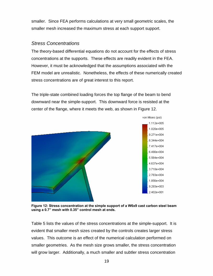
The triple-state combined loading forces the top flange of the beam to bend

downward near the simple-support. This downward force is resisted at the

center of the flange, where it meets the web, as shown in Figure 12.

Figure 12: Stress concentration at the simple support of a W6x9 cast carbon steel beam using a 0.7” mesh with 0.35” control mesh at ends.

Table 5 lists the values of the stress concentrations at the simple-support. It is

evident that smaller mesh sizes created by the controls creates larger stress

values. This outcome is an effect of the numerical calculation performed on

smaller geometries. As the mesh size grows smaller, the stress concentration

will grow larger. Additionally, a much smaller and subtler stress concentration

19

must occur at the fixed support. This fact would explain why stress increase as

mesh sizes grow smaller.

Table 5: Stress concentration values at the simple-support for each beam type and mesh size.

Beam Type Mesh Size Simple-Support Stress

Concentration (psi)

W6x9 0.7” 54,800

W6x9 0.7” mesh w/ 0.35” control at ends 111,200

W10x12 0.7” mesh w/ 0.35” control at ends 89,440

Although this region of high stress has a very interesting effect on the FEA

results, it can be disregarded. In practice it is very unlikely that a beam would be

supported by a theoretical simple-support, across an infinitely small area. As

discussed previously, the restraints applied to the model analyzed in

COSMOSWorks is accompanied by a variety of simplifying assumptions. This

was one of them. To avoid these stress concentrations and provide more

realistic results, SolidWorks models of the actual supports could be drawn and

included in the FEA. However, that investigation is beyond the scope of this

project.

Summary Conclusion Through a theoretical and FEM analysis of a W6x9 fixed/simply-supported beam

under triple-state loading, it is concluded that the beam falls short of the safety

factor requirement. A low-strength W10x12 steel beam is recommended for an

additional cost of $37.50. This beam meets the safety factor criteria while

providing the most cost effective solution. This fact is proven theoretically and

numerically using FEA, under the assumption that the supports are realistic and

practical.

20

Source Code

beamdesign.m

%% Project #1 - Interactive Computation and Graphics of Simple Beams % Scott Moura % SID 15905638 % ME 128, Prof. Lin % Due Wed Feb 22, 2006 %% Nomenclature % A Cross-sectional Area % c Distance from Neutral Axis % cost Material Cost % C Integration Constant % E Young's Modulus % I Moment of Inertia % L Length of Beam % M Bending Moment % M_0 Point Moment % P Point Load % sigma Bending Stress for 3D Distribution % sigma_x Bending Stress % sigma_y Shear Stress % sigma_yield Material Yield Stress % theta Angle of Deflection % u Beam Deflection % V Shear % w Distributed Load % w_x Distributed Load across the beam % W Weight % x Position, from left-end of beam % x_M0 Location of Point Moment % x_P Locaiton of Point Load % x_w1 Location of left-end of distributed load % x_w2 Location of right-end of distributed load clear %% Input Beam Parameters % GUI Input Window prompt = {'Beam Type, Wide-flange [in × lbf/ft]','Beam Length [in]','Distributed Load Intensity [lb/in]',... 'Distributed Load Begins (from fixed end) [in]','Distributed Load Ends (from fixed end) [in]',... 'Point Moment Magnitude (CCW) [in-lb]','Point Moment Location (from fixed end) [in]','Point Load Magnitude [lb]',... 'Point Load Location (from fixed end) [in]','Youngs Modulus [psi]','Yield Stress [psi]','Material Cost [$/lb]','Safety Factor'}; dlg_title = 'Beam Design Parameters'; num_lines= 1; def = {'W6 x 9','120','180','45','100','-1800','30','475','30','29e6','36000','1.25','2'}; answer = inputdlg(prompt,dlg_title,num_lines,def);

21

% Load Beam Data [BeamData,BeamType] = xlsread('BeamData.xls'); BeamType = deblank(BeamType); % Delete Trailing Blank Spaces A = []; for i = 1:length(BeamType) if strcmp(answer{1},BeamType{i}) A = BeamData(i,1); c = (BeamData(i,2))/2; I = BeamData(i,6); tmpidx = findstr(BeamType{i},'x'); W = str2num(BeamType{i}(tmpidx+2:end)); end end if isempty(A) error('Invalid Beam Type') end % Set Variables L = str2num(answer{2}); w = str2num(answer{3}); x_w1 = str2num(answer{4}); x_w2 = str2num(answer{5}); M_0 = str2num(answer{6}); x_M0 = str2num(answer{7}); P = str2num(answer{8}); x_P = str2num(answer{9}); E = str2num(answer{10}); sigma_yield = str2num(answer{11}); cost = str2num(answer{12}); f_S = str2num(answer{13}); %% Evaluate Theoretical Equations % Initiallize Variables x = 0:0.1:L; C = zeros(4,3); w_x = zeros(length(x),4); V = zeros(length(x),4); M = zeros(length(x),4); theta = zeros(length(x),4); u = zeros(length(x),4); % Distributed Load Constants C(1,1) = (3*w)/(4*L^3) * (-1/6*(L-x_w1)^4 + 1/6*(L-x_w2)^4 + L^2*(L-x_w1)^2 - L^2*(L-x_w2)^2); C(2,1) = w/2*(L-x_w1)^2 - w/2*(L-x_w2)^2 - C(1,1)*L; % Point Load Constants C(1,2) = (3*P)/(2*L^3) * (-1/3*(L-x_P)^3 + L^2*(L-x_P)); C(2,2) = P*(L-x_P) - C(1,2)*L; % Point Moment Constants C(1,3) = (3*M_0)/(2*L^3) * ((L-x_M0)^2 - L^2); C(2,3) = -M_0 - C(1,3)*L; % Calculate Beam Property Distributions for i = 1:length(x)

22

% Distributed Load w_x(i,1) = -w * heaviside(x(i)-x_w1,0) + w * heaviside(x(i)-x_w2,0); V(i,1) = -w * heaviside(x(i)-x_w1,1) + w * heaviside(x(i)-x_w2,1) + C(1,1); M(i,1) = -w/2 * heaviside(x(i)-x_w1,2) + w/2 * heaviside(x(i)-x_w2,2) + C(1,1)*x(i) + C(2,1); theta(i,1) = -w/(6*E*I) * heaviside(x(i)-x_w1,3) + w/(6*E*I) * heaviside(x(i)-x_w2,2) + C(1,1)/(2*E*I)*(x(i))^2 + C(2,1)/(E*I)*x(i) + C(3,1); u(i,1) = -w/(24*E*I) * heaviside(x(i)-x_w1,4) + w/(24*E*I) * heaviside(x(i)-x_w2,4) + C(1,1)/(6*E*I)*(x(i))^3 + C(2,1)/(2*E*I)*(x(i))^2 + C(3,1)*x(i) + C(4,1); % Point Force w_x(i,2) = -P * heaviside(x(i)-x_P,-1); V(i,2) = -P * heaviside(x(i)-x_P,0) + C(1,2); M(i,2) = -P * heaviside(x(i)-x_P,1) + C(1,2) * x(i) + C(2,2); theta(i,2) = -P/(2*E*I) * heaviside(x(i)-x_P,2) + C(1,2)/(2*E*I) * (x(i))^2 + C(2,2)/(E*I)*x(i) + C(3,2); u(i,2) = -P/(6*E*I) * heaviside(x(i)-x_P,3) + C(1,2)/(6*E*I)*(x(i))^3 + C(2,2)/(2*E*I)*(x(i))^2 + C(3,2)*x(i) + C(4,2); % Point Moment w_x(i,3) = M_0 * heaviside(x(i)-x_M0,-2); V(i,3) = M_0 * heaviside(x(i)-x_M0,-1) + C(1,3); M(i,3) = M_0 * heaviside(x(i)-x_M0,0) + C(1,3)*x(i) + C(2,3); theta(i,3) = M_0/(E*I) * heaviside(x(i)-x_M0,1) + C(1,3)/(2*E*I)*(x(i))^2 + C(2,3)/(E*I)*x(i) + C(3,3); u(i,3) = M_0/(2*E*I) * heaviside(x(i)-x_M0,2) + C(1,3)/(6*E*I)*(x(i))^3 + C(2,3)/(2*E*I)*(x(i))^2 + C(3,3)*x(i) + C(4,3); end % Distribution Totals (Superpose Equations) w_x(:,4) = w_x(:,1) + w_x(:,2) + w_x(:,3); V(:,4) = V(:,1) + V(:,2) + V(:,3); M(:,4) = M(:,1) + M(:,2) + M(:,3); theta(:,4) = theta(:,1) + theta(:,2) + theta(:,3); u(:,4) = u(:,1) + u(:,2) + u(:,3); % Stress Calculations sigma_x = M(:,4)*c/I; sigma_y = V(:,4)/A; sigma = (sigma_x.^2 + sigma_y.^2).^0.5; [sigma_max, tmpidx] = max(sigma); x_sigma_max = x(tmpidx); % Cost Calculations TotalCost = cost * W * L / 12; %% Analyze Results % Calculate Maximum and Minimum Property Values disp(answer{1}) disp('---------------------------------')

23

[V_max, tmpidx] = max(abs(V(:,4))); V_max = V(tmpidx,4); x_V_max = x(tmpidx); [M_max, tmpidx] = max(abs(M(:,4))); M_max = M(tmpidx,4); x_M_max = x(tmpidx); [theta_max, tmpidx] = max(abs(theta(:,4))); theta_max = theta(tmpidx,4); x_theta_max = x(tmpidx); [u_max, tmpidx] = max(abs(u(:,4))); u_max = u(tmpidx,4); x_u_max = x(tmpidx); % Output Boundary Property Values V_A = ['Sheer at A: ' num2str(V(1,4)) ' lbs']; disp(V_A) V_B = ['Sheer at B: ' num2str(V(end,4)) ' lbs']; disp(V_B) M_A = ['Moment at A: ' num2str(M(1,4)) ' in-lbs']; disp(M_A) M_B = ['Moment at B: ' num2str(M(end,4)) ' in-lbs']; disp(M_B) theta_A = ['Angle of Deflection at A: ' num2str(theta(1,4)) ' rad']; disp(theta_A) theta_B = ['Angle of Deflection at B: ' num2str(theta(end,4)) ' rad']; disp(theta_B) u_A = ['Deflection at A: ' num2str(u(1,4)) ' in']; disp(u_A) u_B = ['Deflection at B: ' num2str(u(end,4)) ' in']; disp(u_B) disp(' ') % Output Maximum and Minimum Property Values maxsheer = ['Maximum Sheer: ' num2str(V_max) ' lbs @ x = ' num2str(x_V_max) ' in']; disp(maxsheer) maxmoment = ['Maximum Moment: ' num2str(M_max) ' in-lbs @ x = ' num2str(x_M_max) ' in']; disp(maxmoment) maxangle = ['Maximum Angle of Deflection: ' num2str(theta_max) ' rad @ x = ' num2str(x_theta_max) ' in']; disp(maxangle) maxdeflect = ['Maximum Deflection: ' num2str(u_max) ' in @ x = ' num2str(x_u_max) ' in']; disp(maxdeflect) maxstress = ['Maximum Stress: ' num2str(sigma_max) ' psi @ x = ' num2str(x_sigma_max) ' in']; disp(maxstress) disp(' ') dispcost = ['Total Cost: $' num2str(TotalCost)]; disp(dispcost)

24

% Create Plots scrsz = get(0,'ScreenSize'); fig1 = figure(1); %set(fig1,'Position',[scrsz(1) scrsz(2) scrsz(3) 0.9*scrsz(4)]) subplot(3,2,1) plot(x,V(:,4)) ylabel('\bfShear, V [lb]') subplot(3,2,2) plot(x,M(:,4)) ylabel('\bfMoment, M [in-lb]') subplot(3,2,3) plot(x,theta(:,4)) ylabel('\bfAngle of Deflection, \theta [rad]') subplot(3,2,4) plot(x,u(:,4)) ylabel('\bfDeflection, u [in]') subplot(3,2,5) plot(x,sigma_x) ylabel('\bfBending Stress, \sigma_x [psi]') xlabel('\bfPosition, x [m]') subplot(3,2,6) plot(x,sigma_y) ylabel('\bfSheer Stress, \sigma_y [psi]') xlabel('\bfPosition, x [m]') % Examine Failure Criteria if (sigma_max > sigma_yield) warnstr = ['The maximum stress (' num2str(sigma_max) ' psi) has exceeded the yield stress value (' num2str(sigma_yield) ' psi). Please reconsider your beam design parameters.']; warndlg(warnstr,'Beam Failure') elseif (sigma_max*f_S) > sigma_yield warnstr = ['The beam does not satisfy the prescribed safety factor of ' num2str(f_S) '. Please reconsider your beam design parameters.'] ; warndlg(warnstr,'Safety Factor not satisfied') end %% Calculate 3D Stress Distribution y = 0:0.1:c; for i = 1:length(x) for j = 1:length(y) sigma_col(j,i) = abs(M(i,4)*y(j)/I); end end figure(2) surf(x,y,sigma_col,'LineStyle','none') colorbar view(0,90) xlabel('Beam Length, x [in]') ylabel('Beam Depth, c [in]')

25

heaviside.m

function y = heaviside(x,n) % HEAVISIDE % Returns x^n if x is positive and zero if x is negative if (x > 0) if n >= 0 y = x^n; else y = 0; end else y = 0; end

26