Interactive Simulation of Fire

Zeki Melek John Keyser

Department of Computer ScienceTexas A&M University

College Station, TX 77843-3112, USAE-mail: z0m8905@cs.tamu.edu

Phone: (979) 845-5007Fax: (979) 847-8578

Technical Report 2002-7-1

July 15, 2002

Abstract

In this paper we describe a fast and interactive model to simulate and control the fire phenomenon.We use a modified interactive fluid dynamics solver to describe the motion of a 3-gas system. Wesimulate the motion of oxidizing air, fuel gases, and exhaust gases. The burning process is simulatedby consuming fuel and air based on the amounts of fuel and air inside each grid cell. The combustionprocess produces heat, and we model the resulting spread of temperature through the system. The heatdistribution induces convection currents in the air, causing the flame to take the appropriate shape. Bymodeling heat distribution, we also simulate the spread of fire to and self-ignition in other combustiblesolids.

Key Words: Physically based modeling, fire simulation, fluid dynamics

1. Introduction

There has been an increasing interest within the computer graphics community for simulation andvisualization of natural phenomena such as water and smoke motion. These physical simulations play anincreasingly important role as a part of the story within the motion picture and game industries, and canbe important cues in applications such as military training. Generally, these applications require visuallycompelling but not strictly accurate models. However, the models need to be capable of capturing thevisual characteristics of the phenomenon, and still be interactive and easy to choreograph. In this paper,we focus on the simulation of fire.

Recently, a number of advances have made realistic interactive modeling of smoke and other gaseousphenomena possible. These coarse-grid fluid-dynamic equation solvers are capable of capturing finescale swirling motion of the air, with a very small computational cost.

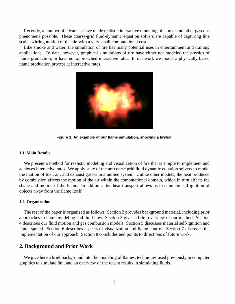
Like smoke and water, the simulation of fire has many potential uses in entertainment and trainingapplications. To date, however, graphical simulations of fire have either not modeled the physics offlame production, or have not approached interactive rates. In our work we model a physically basedflame production process at interactive rates.

Figure 1. An example of our flame simulation, showing a fireball

1.1. Main Results

We present a method for realistic modeling and visualization of fire that is simple to implement andachieves interactive rates. We apply state of the art coarse grid fluid dynamic equation solvers to modelthe motion of fuel, air, and exhaust gasses in a unified system. Unlike other models, the heat producedby combustion affects the motion of the air within the computational domain, which in turn affects theshape and motion of the flame. In addition, this heat transport allows us to simulate self-ignition ofobjects away from the flame itself.

1.2. Organization

The rest of the paper is organized as follows. Section 2 provides background material, including priorapproaches to flame modeling and fluid flow. Section 3 gives a brief overview of our method. Section4 describes our fluid motion and gas combustion models. Section 5 discusses material self-ignition andflame spread. Section 6 describes aspects of visualization and flame control. Section 7 discusses theimplementation of our approach. Section 8 concludes and points to directions of future work.

2. Background and Prior Work

We give here a brief background into the modeling of flames, techniques used previously in computergraphics to simulate fire, and an overview of the recent results in simulating fluids.

2

2.1. Models of Flames

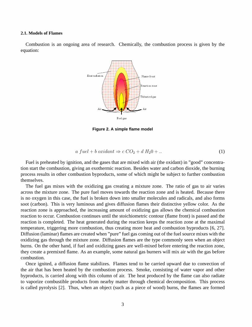
Combustion is an ongoing area of research. Chemically, the combustion process is given by theequation:

Figure 2. A simple flame model

a fuel + b oxidant ⇒ c CO2 + d H20 + .. (1)

Fuel is preheated by ignition, and the gases that are mixed with air (the oxidant) in ”good” concentra-tion start the combustion, giving an exothermic reaction. Besides water and carbon dioxide, the burningprocess results in other combustion byproducts, some of which might be subject to further combustionthemselves.

The fuel gas mixes with the oxidizing gas creating a mixture zone. The ratio of gas to air variesacross the mixture zone. The pure fuel moves towards the reaction zone and is heated. Because thereis no oxygen in this case, the fuel is broken down into smaller molecules and radicals, and also formssoot (carbon). This is very luminous and gives diffusion flames their distinctive yellow color. As thereaction zone is approached, the increasing amount of oxidizing gas allows the chemical combustionreaction to occur. Combustion continues until the stoichiometric contour (flame front) is passed and thereaction is completed. The heat generated during the reaction keeps the reaction zone at the maximaltemperature, triggering more combustion, thus creating more heat and combustion byproducts [6, 27].Diffusion (laminar) flames are created when ”pure” fuel gas coming out of the fuel source mixes with theoxidizing gas through the mixture zone. Diffusion flames are the type commonly seen when an objectburns. On the other hand, if fuel and oxidizing gases are well-mixed before entering the reaction zone,they create a premixed flame. As an example, some natural gas burners will mix air with the gas beforecombustion.

Once ignited, a diffusion flame stabilizes. Flames tend to be carried upward due to convection ofthe air that has been heated by the combustion process. Smoke, consisting of water vapor and otherbyproducts, is carried along with this column of air. The heat produced by the flame can also radiateto vaporize combustible products from nearby matter through chemical decomposition. This processis called pyrolysis [2]. Thus, when an object (such as a piece of wood) burns, the flames are formed

3

from combustible portions of the object being vaporized and then oxidizing in the region just beyond thesurface.

The color of a flame in the reaction zone is determined by the energy released in the exothermicoxidation process. Thus, a ”pure” burning chemical may emit a single wavelength of light, while a morecomplex substance (e.g. wood) may emit at numerous wavelengths. In addition, the heat generated bycombustion can cause combustion materials to emit light in form of thermal radiation [2, 27].

2.2. Flame Modeling in Computer Graphics

Within the computer graphics community, early models of fire include those of Reeves and Perlin.Reeves’s approach [20], using particle systems, requires a very large number of particles to hide thepointillistic nature of the technique, and is thus computationally expensive. Perlin’s approach [17, 18]uses a procedural noise function, which has problems including external forces such as wind into thesimulation. Inakage [11] uses a physical model to emit light in the regions of combustion, but his modelis computationally expensive and deals with still images rather than multiple animated flames.

More recently, Chiba et al. [4] and Takahashi et al. [26] both use a gridded representation of the space,where each grid cell contains a certain amount of fuel gas and heat. This is similar to our representation.Fire itself is modeled by placing geometric primitives around particle trajectories, which are influencedby a vector field. Perry and Picard [19] have a similar representation for the flames. They reuse thesame polygons used for modeling to spread the fire. The flame front is represented by a set of particles,adding new particles as the front expands. Stam and Fiume [24] use a map covering the object definingthe amount of fuel and temperature on every point on the object. Fire animation is done using turbulentwind fields [23] and rendering is based on warped blobs. The approach is costly and user controls arenot so flexible and intuitive.

Beaudin et al. [1] use a similar but more accurate flame front technique to model the spreading ofthe flames. They guarantee that the boundary lies on the object, unlike Perry and Picard’s work. Theyplant the root of the flame skeleton on the surface and displace the skeleton with the air vector field.They use an implicit surface representation to dress up the flame skeletons during the rendering. Theirmethod is fast, interactive, and allows for quick preview, but lacks accurate air and smoke motion insidethe simulation volume.

Yngve et al. [28] proposed a solution for the compressible version of the fluid flow equations, mod-eling the shock waves created by explosions, but it includes strict time step restrictions, making thesolution computationally expensive. A recent paper Nguyen et al. [16] treats two phase incompressibleflow where one phase is being converted into the other, e.g. vaporization of liquid water.

The spread of fire has been another area of research. NIST has developed the CFAST fire simula-tor [12]. CFAST gives an accurate simulation of the impact of fire and its byproducts, but operates inbatch mode, providing the user graphs and data dumps as output. Bukowski and Squin [3] have inte-grated CFAST and the Berkeley Architectural Walkthru program, making the results of CFAST moreunderstandable. However, the aim of this work is not to create visually appealing images, and the firesimulation itself is done offline.

Finally, two fire-related papers are scheduled to be presented at Siggraph 2002[14, 15]. The authorsare not releasing these papers at this time, however, and so we cannot compare our approach to theirs.

4

2.3. Modeling Fluid Flow

Our model is based on the direct simulation of the incompressible fluid dynamic equations on coarsegrids. Kajiya and Von Herzen [13] worked on very coarse grids, using the very limited computer powerthey had at that time. Foster and Metaxas [8, 9] reintroduced the method to the CG community, andwere able to capture nice swirling motions using relatively coarse grids. Their model used an explicitintegration scheme, bounding their time step in order to keep the simulation stable. They also use acostly relaxation step to ensure mass conservation. Yoshida et al. [29] used smoke particles (puffs) tomodel the motion of the smoke and vorticity fields to take obstacles into account. Stam [21, 22] useda semi-Lagrangian advection scheme and implicit solver to make the simulation unconditionally stable;even large time steps are allowed in his Stable Fluids model. He also used pressure-Poisson equationsto conserve mass. Because he used a first order integration scheme, these simulations suffered fromnumerical dissipation. Fedkiw at al. [7] included vorticity confinement in the Stable Fluids model,keeping the smoke “alive” and increasing the quality of the flow with a very small amount of additionalcomputational cost. The Stable fluids model can handle boundaries inside the computational domain.

2.4. Stable Fluids

To model the fluid flow, we use a modified version of Stam’s Stable Fluids approach. We providea brief overview of the method here, but the reader is encouraged to refer to the original reference formore details [21].

Compressible flow equations introduce a very strict time step restriction associated with the acousticwaves. To avoid this strict restriction incompressible flow equations are preferred whenever possible.When the speed of the flow is below the speed of sound, the compression effects are negligible [7].Using coarse grids also lets us neglect viscous effects, which occur at a scale far below our grid cell size.In compact form, the incompressible Navier-Stokes equations governing fluid flow are as follows:

∇ · u = 0 (2)

∂u

∂t= f − (u · ∇)u−∇p (3)

whereu is the velocity field, andp is a pressure field. Eq. 2 describes incompressibility, hencedivergence free flow, and Eq. 3 describes fluid flow. Looking at Eq. 3 more closely,f is the externalforce, including buoyancy and gravity forces. The second term is the nonlinear part of the Navier-Stokesequation - it is the advection of the velocity field on itself. The last term accounts for the pressureinduced motion. The solution of the equations involves three main steps:

• The first step determines the force term. More about the force is described below, but briefly wefind the buoyancy force based on the temperature and the gravity force based on the amount offuel and exhaust gas densities in each grid cell.

• The second step advects the velocity field itself to the next time step. A particle at each cell centeris traced back in time over the time step and the new velocity for the cell is the interpolation of thevelocities that the particle had a time step ago.

5

•

∇2p =1

∆t∇ · u (4)

The third step combines Eq. 2 and 3 and makes the velocity field divergence free and incompress-ible using a projection method [5]. The vector field found in previous steps is made incompressibleby subtracting the gradient of the pressure. The pressure is found by solving the Poisson equation(Eq. 4) with the Neumann boundary condition. The Poisson equation becomes a sparse linear sys-tem, making the implementation straightforward, using multigrid methods such as the conjugategradient [10, 25].

A non-reactive substance like smoke is advected at the same time with the fluid:

∂a

∂t= −(u · ∇)a− αaa + Sa (5)

whereαa is a dissipation rate andSa is a source term. Since Eqs. 3 and 5 have identical structure, thesame source code can be reused.

3. Overview of Our Method

In our model, we transport the fuel and exhaust gases with the motion of the air, creating a dynamic3-gas system. Heat is also transported with the flow of the air, enabling us to model heat distributioninside the computational domain more accurately than any other known fire model. Heat affects thebuoyancy forces and changes the flow accordingly. Sufficient heat and an appropriate mixture of the airand fuel gas creates a combustion reaction, releasing smoke and more heat into the system. Under thecorrect conditions, a stable flame front is produced. With insufficient heat, oxidizing gas, or fuel, theflame is not sustainable, and dies out, as one would hope.

Transporting the heat within the system allows us to pyrolyse material inside the computational do-main. Thus, we can model self ignition of the material even if it is away from the flame. Among the keyassumptions and simplifications we make are:

• The fuel gas is uniform. That is, we assume that fuel is either burned or unburned, that anycombustible byproducts behave exactly the same as the original fuel, and that the amount of heatproduced is a function of just the amount of fuel burned.

• We assume that the viscosity of the mixed gas system is negligible. Although different ratios ofmixed gasses will have different viscosities, we assume that any effects of this are too small to beseen over a coarse grid.

• The compression of the gases as a result of combustion is ignored. Simulating a compressiblefluid is significantly more difficult than an incompressible fluid, and it is unlikely that a simulationof compressible fluids could be achieved at interactive rates. Furthermore, since we are simulatingbasically stable flames (i.e. not explosive situations), it is unlikely that this compression will havea significant visual effect on the solution. The total amount of gas (fuel, oxidizer, and exhaust) ina unit volume is assumed to be constant.

6

• Heat and temperature are treated interchangeably. While this is reasonable for a single gas, amixed-gas system would not necessarily behave this way, however we assume the difference isminimal.

• The pressure effects of gases at different temperatures are not modeled directly (see the bulletabout compression). However, the most significant effects (buoyancy of hot air, spread of heatthrough the fluid) are modeled.

4. Simulating the Flame

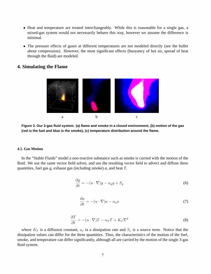
a b c

Figure 3. Our 3-gas fluid system. (a) flame and smoke in a closed environment, (b) motion of the gas(red is the fuel and blue is the smoke), (c) temperature distribution around the flame.

4.1. Gas Motion

In the ”Stable Fluids” model a non-reactive substance such as smoke is carried with the motion of thefluid. We use the same vector field solver, and use the resulting vector field to advect and diffuse threequantities, fuel gasg, exhaust gas (including smoke)a, and heatT.

∂g

∂t= −(u · ∇)g − αgg + Sg (6)

∂a

∂t= −(u · ∇)a− αaa (7)

∂T

∂t= −(u · ∇)T − αT T + KT∇2 (8)

whereKT is a diffusion constant,ax ia a dissipation rate andSx is a source term. Notice that thedissipation values can differ for the three quantities. Thus, the characteristics of the motion of the fuel,smoke, and temperature can differ significantly, although all are carried by the motion of the single 3-gasfluid system.

7

For fuel gasesag is small if not zero, whereas smoke has a largeraa. Sg is initially empty, except theinitial source flame. During the simulation as objects start burning, they too become sources. Smoke andtemperature do not have source terms, since smoke and heat comes from the burning process, accordingto the amount of fuel and air consumed within one time step.

Temperature has a largeKT which simulates diffusion of the heat and smallaT value, diffusing fastbut not dissipating within the system. Diffusion of the temperature field is solved with a similar approachused in [21], using an implicit integration step, which gives a sparse linear system when discretized.

The fluid system is modified by the presence of the fuel, exhaust gas, and temperature. Referring toEq. 3, the external force,F, acting in any one cell is given by:

F = fg(gg + da)

00−1

+ fT (T − Tamb)

001

(9)

wherefg andfT are positive constants controlling the force components based on gravity and tem-perature respectively, andTamb is the room temperature. Hot air will thus rise, and cold air fall, creatingconvection currents necessary to give the correct flame shape. The smoke and fuel gas will tend to fall,though this effect is usually not very noticeable (i.e.fg should be fairly small).

4.2. Combustion

The combustion (burning) in a cell is defined by:if T > Tthreshold

C = r min(dA, b dg) (10)

∂dg

∂t= −C

b(11)

∂da

∂t= C

(1 +

1

b

)(12)

∂T

∂t= T0C (13)

wheredx is the density,r is the burning rate (0 < r ≤ 1), b is the stoichiometric mixture (the amountof air required to burn one unit of fuel),Tthreshold is the lower flammability temperature where burningcan occur, andT0 is the output heat from the reaction. The burning rate is the percentage of the gas thatcan be burned in a second. Oxygen densitydA is defined as

D = dA + dg + da (14)

8

whereD is the total amount of gas in each cell, which is constant. If there is no fuel or smoke thenit is filled with oxygen, and vice versa. Note that although air is not all oxygen, this can be easilyaccounted for by adjusting the stoichiometric mixture appropriately. At this stage we only have modeledone reaction which is controlled with the reaction ratio.

Conceptually, the combustion inside the cell is controlled with 4 parameters.Tthreshold is straightfor-ward. b controls oxygen requirement of the combustion and can be used to model different reactions.T0 controls the intensity of the reaction.r controls how quickly the gas can be burned. The heat outputcoming from a combustion cell can be sufficient to start a reaction in a neighboring cell. Or it mightnot be sufficient and the combustion reaction cannot continue, extinguishing the flame. Using theseparameters, the shape and the stability of the flame can be controlled. Examples are shown in Section 7.

4.3. Creating a Flame

To achieve a steady flame, we simulate the effects of ignition. Initially temperature is constant andlow and there is no smoke or fuel gas in the system. Initial fuel sources start to provide fuel gas to thesystem. Note that this fuel source may be a gaseous source, such as a gas jet, or may be the result ofpyrolysis from a solid, such as a log (see section 5). Since there is no reaction yet, all the motion comesfrom the initial velocity of the gas coming from the fuel source, if there is any. Fuel gas coming out of thesource is advected within the system. The fuel gas is ignited either by reaching a sufficient temperature,or by a special “ignition” step. In the ignition step, we temporarily setTthreshold to 0 for the durationof the time step, simulating an ignition of the fuel (alternatively, we could increase the temperature inone cell for one time step). Assuming there is a mixture of fuel and air in a cell, combustion will occur.This combustion increases the heat in the system and can provide enough heat to the neighboring cellsto continue the burning process on the next time step. Hot air rises due to the buoyancy force, and soonthe flame stabilizes. Smoke is produced as a by-product of the combustion, and tends to rise with the hotair produced by the flame.

There are several possible reasons a flame might not stabilize. If the fuel and air has not mixedat ignition, no burning can occur. If an insufficient amount of fuel is present, too little heat may begenerated to sustain the burning. Likewise, if the output heat from the reaction is too low, the heatproduced might not be enough to propagate combustion and thereby sustain a flame.

5. Representing Solids and Flame Spread

Solid materials inside the computational domain are voxelized and the corresponding grid cells in thecomputational domain are marked as filled. This filled/empty information is used in flow calculations[21, 7]. In the advection step, the particle tracer hits and stops on filled grid cells, and in the diffusionstep the filled grid cells are assigned the same amount of density as their empty neighbor, making theincoming and outgoing density flows equal. If a filled grid cell has more than one empty neighbor,average values are used, but it is possible for material one voxel thick to ”leak”.

Each filled grid cell is a potential fuel source. Active fuel sources emit fuel gas density into the neigh-boring unfilled cells at every time step. Potential fuel sources can later self-ignite, becoming active fuelsources. Every filled grid cell has a pyrolysis temperature, which is a material property (nonflammablematerials simply have an arbitrarily high pyrolysis temperature). When a filled grid cell reaches itspyrolysis temperature, it becomes a fuel source. Since the self ignition temperature of the fuel is gener-

9

ally much smaller than the pyrolysis temperature, if there is enough air around, the resulting fuel startsburning once it mixes with air.

As mentioned before, we maintain a temperature value at each grid cell. Heat propagation is modeledwithin a solid object using the well-known heat flow equation:

∂T

∂t= k∇2T (15)

wherek is the diffusivity constant for the material. For the unfilled cells, heat both diffuses through thesystem and advects along with the gas flow. Thus, we have temperature values at the boundary betweenthe solid and the air. These temperatures serve as boundary conditions when solving the differentialequation.

Thus, we can transport heat through both the air (via the fluid solver) and the solid objects in thescene. Heat from the burning gas warms the air, which moves around, possibly heating up other solidsin the scene. If these solids reach a high enough temperature, they will begin pyrolysis, becoming activefuel sources and spewing more gases, which will likely combust.

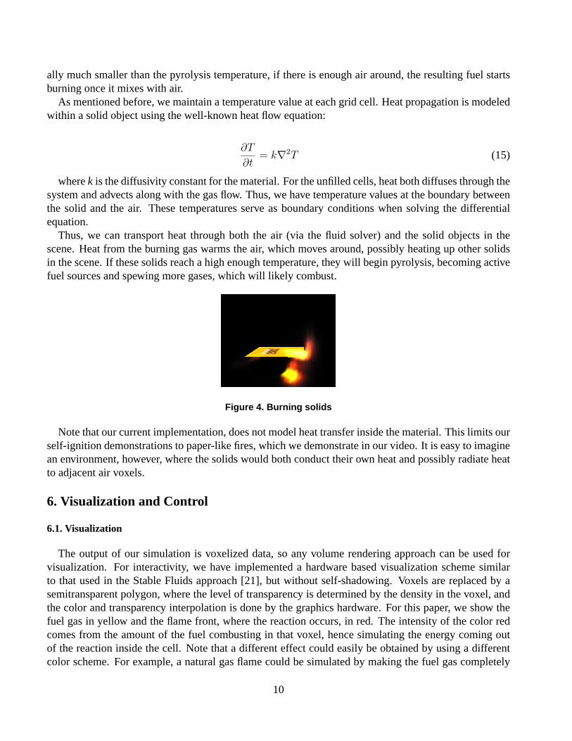
Figure 4. Burning solids

Note that our current implementation, does not model heat transfer inside the material. This limits ourself-ignition demonstrations to paper-like fires, which we demonstrate in our video. It is easy to imaginean environment, however, where the solids would both conduct their own heat and possibly radiate heatto adjacent air voxels.

6. Visualization and Control

6.1. Visualization

The output of our simulation is voxelized data, so any volume rendering approach can be used forvisualization. For interactivity, we have implemented a hardware based visualization scheme similarto that used in the Stable Fluids approach [21], but without self-shadowing. Voxels are replaced by asemitransparent polygon, where the level of transparency is determined by the density in the voxel, andthe color and transparency interpolation is done by the graphics hardware. For this paper, we show thefuel gas in yellow and the flame front, where the reaction occurs, in red. The intensity of the color redcomes from the amount of the fuel combusting in that voxel, hence simulating the energy coming outof the reaction inside the cell. Note that a different effect could easily be obtained by using a differentcolor scheme. For example, a natural gas flame could be simulated by making the fuel gas completely

10

transparent, and the combustion region blue. Generally, we prefer not to show most of the smoke, makingit almost transparent, so as not to obscure the flame. As the objects near their pyrolysis temperature theircolor is darkened to simulate charring [19].

The focus of our work has been on developing an interactive model, hence the visual quality is ofsecondary concern. Although the approach described works well for interactive visualization, higherquality images may be desired. If the restriction on interactivity is released, a larger grid size can alsobe used, giving more complex flame behavior. A low grid resolution and large time step interactivesimulation can be used to choreograph the scene and then a smaller time step-larger grid solution can berendered for better images.

6.2. Control of Flame Shape

In order to simulate different burning reactions, it is important for an animator to have some controlover the flame shape. The shape of the flame can be controlled by modifying a few key parameters:

• Turbulence controls the amount of additional random motion added to the fluid motion field. Ifzero, the flame will eventually stabilize in a fixed shape. Introducing turbulence causes the flameto have a more realistic motion.

Figure 5. The flame at left experiences no turbulence whereas the right flame does. The flame at leftwill remain in that shape, while the one on the right will change over time.

• Burn rate gives the amount of fuel that can be burned in one second, as a percentage of the max-imum amount of fuel that can combust (i.e. is at an adequate temperature and is mixed with airappropriately). Large (=1.0) burning rates tend to create very thin and sharp flames, since fuel isusually consumed soon after mixing with air, while slower burning rates create larger and moreblurry flames.

Figure 6. The flame at left has a faster burning rate than the one at right.

11

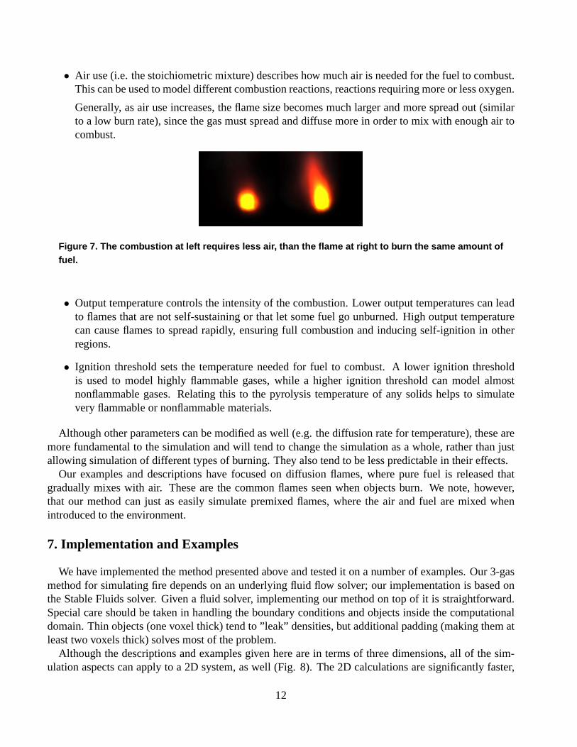
• Air use (i.e. the stoichiometric mixture) describes how much air is needed for the fuel to combust.This can be used to model different combustion reactions, reactions requiring more or less oxygen.

Generally, as air use increases, the flame size becomes much larger and more spread out (similarto a low burn rate), since the gas must spread and diffuse more in order to mix with enough air tocombust.

Figure 7. The combustion at left requires less air, than the flame at right to burn the same amount offuel.

• Output temperature controls the intensity of the combustion. Lower output temperatures can leadto flames that are not self-sustaining or that let some fuel go unburned. High output temperaturecan cause flames to spread rapidly, ensuring full combustion and inducing self-ignition in otherregions.

• Ignition threshold sets the temperature needed for fuel to combust. A lower ignition thresholdis used to model highly flammable gases, while a higher ignition threshold can model almostnonflammable gases. Relating this to the pyrolysis temperature of any solids helps to simulatevery flammable or nonflammable materials.

Although other parameters can be modified as well (e.g. the diffusion rate for temperature), these aremore fundamental to the simulation and will tend to change the simulation as a whole, rather than justallowing simulation of different types of burning. They also tend to be less predictable in their effects.

Our examples and descriptions have focused on diffusion flames, where pure fuel is released thatgradually mixes with air. These are the common flames seen when objects burn. We note, however,that our method can just as easily simulate premixed flames, where the air and fuel are mixed whenintroduced to the environment.

7. Implementation and Examples

We have implemented the method presented above and tested it on a number of examples. Our 3-gasmethod for simulating fire depends on an underlying fluid flow solver; our implementation is based onthe Stable Fluids solver. Given a fluid solver, implementing our method on top of it is straightforward.Special care should be taken in handling the boundary conditions and objects inside the computationaldomain. Thin objects (one voxel thick) tend to ”leak” densities, but additional padding (making them atleast two voxels thick) solves most of the problem.

Although the descriptions and examples given here are in terms of three dimensions, all of the sim-ulation aspects can apply to a 2D system, as well (Fig. 8). The 2D calculations are significantly faster,

12

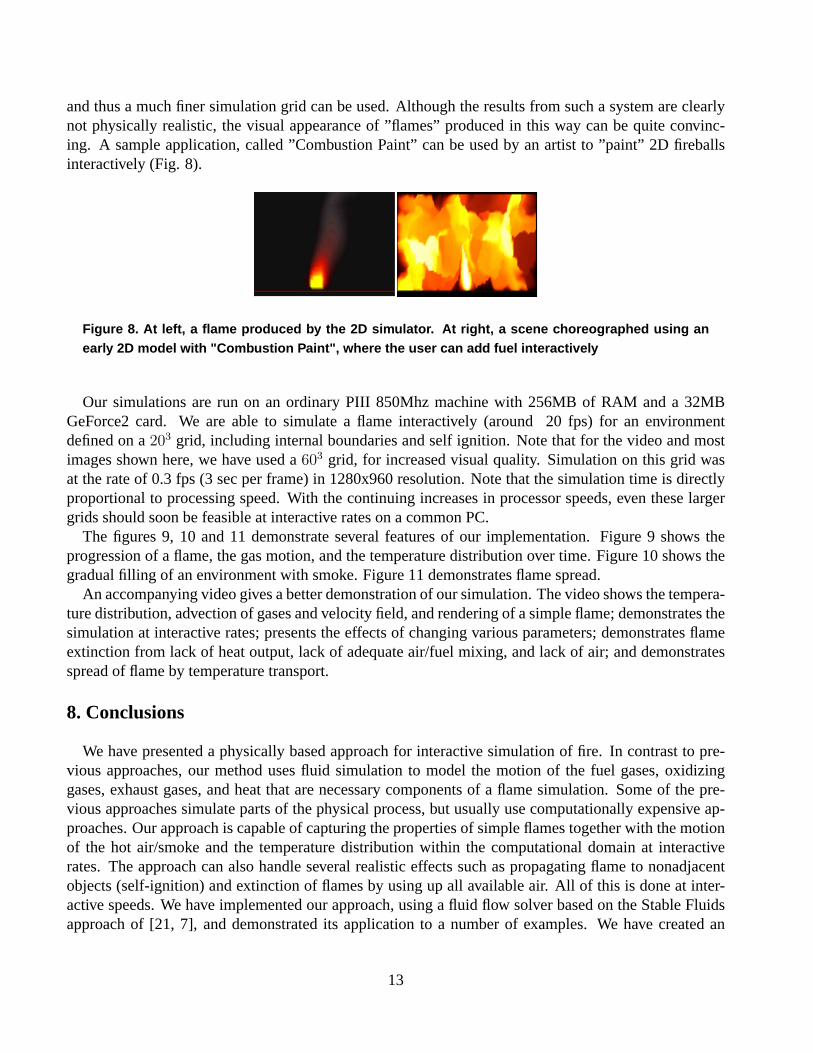
and thus a much finer simulation grid can be used. Although the results from such a system are clearlynot physically realistic, the visual appearance of ”flames” produced in this way can be quite convinc-ing. A sample application, called ”Combustion Paint” can be used by an artist to ”paint” 2D fireballsinteractively (Fig. 8).

Figure 8. At left, a flame produced by the 2D simulator. At right, a scene choreographed using anearly 2D model with "Combustion Paint", where the user can add fuel interactively

Our simulations are run on an ordinary PIII 850Mhz machine with 256MB of RAM and a 32MBGeForce2 card. We are able to simulate a flame interactively (around 20 fps) for an environmentdefined on a203 grid, including internal boundaries and self ignition. Note that for the video and mostimages shown here, we have used a603 grid, for increased visual quality. Simulation on this grid wasat the rate of 0.3 fps (3 sec per frame) in 1280x960 resolution. Note that the simulation time is directlyproportional to processing speed. With the continuing increases in processor speeds, even these largergrids should soon be feasible at interactive rates on a common PC.

The figures 9, 10 and 11 demonstrate several features of our implementation. Figure 9 shows theprogression of a flame, the gas motion, and the temperature distribution over time. Figure 10 shows thegradual filling of an environment with smoke. Figure 11 demonstrates flame spread.

An accompanying video gives a better demonstration of our simulation. The video shows the tempera-ture distribution, advection of gases and velocity field, and rendering of a simple flame; demonstrates thesimulation at interactive rates; presents the effects of changing various parameters; demonstrates flameextinction from lack of heat output, lack of adequate air/fuel mixing, and lack of air; and demonstratesspread of flame by temperature transport.

8. Conclusions

We have presented a physically based approach for interactive simulation of fire. In contrast to pre-vious approaches, our method uses fluid simulation to model the motion of the fuel gases, oxidizinggases, exhaust gases, and heat that are necessary components of a flame simulation. Some of the pre-vious approaches simulate parts of the physical process, but usually use computationally expensive ap-proaches. Our approach is capable of capturing the properties of simple flames together with the motionof the hot air/smoke and the temperature distribution within the computational domain at interactiverates. The approach can also handle several realistic effects such as propagating flame to nonadjacentobjects (self-ignition) and extinction of flames by using up all available air. All of this is done at inter-active speeds. We have implemented our approach, using a fluid flow solver based on the Stable Fluidsapproach of [21, 7], and demonstrated its application to a number of examples. We have created an

13

interactive hardware-based OpenGL renderer that, while not producing “eyecatching” visualizations, isable to show the strength of our model.

There are numerous avenues for expanded research on this topic. Four directions of future work thatwe intend to explore are the following:

• Though we have presented an approach for modeling heat transport within the solid objects, wehave not implemented this yet (though it should be straightforward to do so). Along with this,a more advanced model of fuel output and consumption within solids could be used to simulatecharring and decomposition of the objects themselves over time.

• Our assumption that the sum of the air, fuel, and exhaust gas in a cell is constant is somewhatunrealistic. Treating air as independent of fuel and exhaust will yield more accurate results, par-ticularly for special cases such as consuming all of the air in the room. However, making such achange may necessitate accounting for changes in pressure or gas compression, which may causethe simulation to become too slow.

• Although the parameter values we discuss provide a great deal of control over the flame, it wouldbe useful to provide a more intuitive and complete set of controls for use by animators. For thesame reason, incorporating our implementation into a higher-quality rendering system (e.g. avolume ray-tracer, light emission model) would allow better pictures to be produced.

• Visual quality has not been the focus of this work, and thus there are many ways to improve the vi-sualization. Among the improvements we would like to make are incorporation of a light emissionmodel with a photon map renderer, adding (as a postprocess) a flame skeleton [1] or particle-based[20] approach to provide fine detail, and creating a better model for the luminance via thermal ra-diation of unburned fuel and actual combustion. We believe that incorporating such renderingimprovements will result in images that are competitive with any other flame visualization.

References

[1] P. Beaudin, S. Parquet, and P. Poulin. Realistic and controllable fire simulation.In Proceedings of GraphicsInterface 2001, pages 159–166, 2001.

[2] R. Borghi, M. Destriau, and G. De Soete.Combustion and flames, chemical and physical principles. EditionsTechnip, Paris, 1995.

[3] R. Bukowski and C. Sequin. Interactive simulation of fire in virtual building environments.In Proceedingsof SIGGRAPH 97, Computer Graphics Proceedings, Annual Conference Series, ACM, 1997.

[4] N. Chiba, K. Muraoka, and M. Miura. Two dimensional visual simulation of flames, smoke and the spreadof fire. The Journal of Visualization and Computer Animation, (5(1)):37–54, 1994.

[5] A. Chorin. A numerical method for solving incompressible viscous flow problems.Journal of Computa-tional Physics, (2):12–26, 1967.

[6] C. Detienne.Physical Development of Natural and Criminal Fires. Charles C. Thomas, 1994.[7] R. Fedkiw, J. Stam, and W. Jensen, H. Visual simulation of smoke.In Proceedings of SIGGRAPH 01,

Computer Graphics Proceedings, Annual Conference Series, ACM, pages 15–22, 2001.[8] N. Foster and D. Metaxas. Realistic animation of liquids.Graphical Models and Image Processing,

(58(5)):471–483, 1996.[9] N. Foster and D. Metaxas. Modeling the motion of a hot turbulent gas.In Proceedings of SIGGRAPH 97,

Computer Graphics Proceedings, Annual Conference Series, ACM, pages 181–188, 1997.

14

[10] W. Hackbusch.Multi-grid methods and applications. Springer Verlag, Berlin, 1985.[11] M. Inakage. A simple model of flames.In Proceedings of CG international, pages 71–81, 1990.[12] W. Jones, W, P. Forney, G, D. Peacock, R, and A. Reneke, P. A technical reference for cfast: An engineering

tool for estimating fire and smoke transport. 2000.[13] T. Kajiya, J and P. Von Herzen, B. Ray tracing volume densities.In Computer Graphics (Proceedings of

SIGGRAPH 89), (18(3)):165–174, 1984.[14] A. Lamorlette and N. Foster. Structural modeling of natural flames.In Proceedings of SIGGRAPH 02,

Computer Graphics Proceedings, Annual Conference Series, ACM, 2002. to appear.[15] D. Nguyen, P. Fedkiw, R, and W. Jensen, H. Physically based modeling and animation of fire.In Proceedings

of SIGGRAPH 02, Computer Graphics Proceedings, Annual Conference Series, ACM, 2002. to appear.[16] Q. Nguyen, D, R. Fedkiw, and M. Kang. A boundary condition capturing method for incompressible flame

discontinuities.Journal of Computational Physics, (172):179–198, 2001.[17] H. Perlin, K. An image synthesizer.In Computer Graphics (Proceedings of SIGGRAPH 85), ACM,

(19(3)):287–296, 1985.[18] H. Perlin, K and M. Hoffert, E. Hypertexture.In Computer Graphics (Proceedings of SIGGRAPH 89),

ACM, (23(3)):253–262, 1989.[19] H. Perry, C and W. Picard, R. Synthesizing flames and their spreading.In Proceedings of Fifth Eurographics

Workshop on Animation and Simulation, pages 105–117, 1994.[20] T. Reeves, W. Particle systems - a technique for modeling a class of fuzzy objects.ACM Transactions on

Graphics, (2(2)), 1983.[21] J. Stam. Stable fluids.In Proceedings of SIGGRAPH 99, Computer Graphics Proceedings, Annual Confer-

ence Series, ACM, pages 121–128, 1999.[22] J. Stam. Interacting with smoke and fire in real time.Communications of the ACM, (43(7)):77–83, 2000.[23] J. Stam and E. Fiume. Turbulent wind fields for gaseous phenomena.In Proceedings of SIGGRAPH 93,

Computer Graphics Proceedings, Annual Conference Series, ACM, pages 369–376, 1993.[24] J. Stam and E. Fiume. Depicting fire and other gaseous phenomena using diffusion process.In Proceedings

of SIGGRAPH 95, Computer Graphics Proceedings, Annual Conference Series, ACM, pages 129–136, 1995.[25] N. Swarztrauber, P and A. Sweet, R. Efficient fortran subprograms for the solution of separable elliptic

partial differential equations.ACM Transactions on Mathematical Software, (5(3)):352–364, 1979.[26] J. Takahashi, H. Takahashi, and N. Chiba. Image synthesis of flickering scenes including simulated flames.

IEICE Transactions on Information Systems, (E80-D(11)):1102–1108, 1997.[27] WebSite.Online Class Notes, CPE630, http://eyrie.shef.ac.uk/will/eee/. University of Sheffield, 2002.[28] D. Yngve, G, F. O’Brien, J, and K. Hodgins, J. Animating explosions.In Proceedings of SIGGRAPH 00

Computer Graphics Proceedings, Annual Conference Series, ACM, pages 29–36, 2000.[29] S. Yoshida and T. Nishita. Modelling of smoke flow taking obstacles into account.Proc.of the 8th Pacific

Conference, pages 135–144, 2000.

15

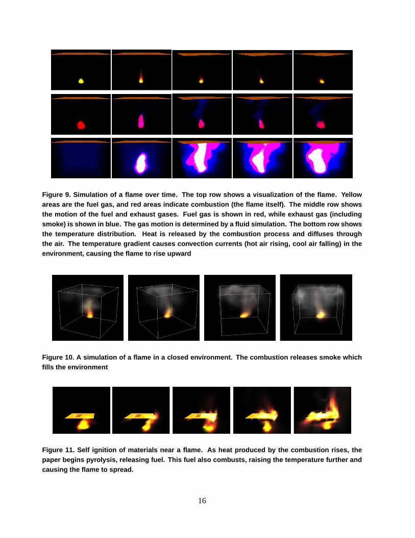
Figure 9. Simulation of a flame over time. The top row shows a visualization of the flame. Yellowareas are the fuel gas, and red areas indicate combustion (the flame itself). The middle row showsthe motion of the fuel and exhaust gases. Fuel gas is shown in red, while exhaust gas (includingsmoke) is shown in blue. The gas motion is determined by a fluid simulation. The bottom row showsthe temperature distribution. Heat is released by the combustion process and diffuses throughthe air. The temperature gradient causes convection currents (hot air rising, cool air falling) in theenvironment, causing the flame to rise upward

Figure 10. A simulation of a flame in a closed environment. The combustion releases smoke whichfills the environment

Figure 11. Self ignition of materials near a flame. As heat produced by the combustion rises, thepaper begins pyrolysis, releasing fuel. This fuel also combusts, raising the temperature further andcausing the flame to spread.

16