interest point descriptors and matching
DESCRIPTION
Interest Point Descriptors and Matching. CS485/685 Computer Vision Dr. George Bebis. Eliminate rotational ambiguity. Compute appearance descriptors. Extract affine regions. Normalize regions. SIFT (Lowe ’04). Interest Point Descriptors. Descriptors. Simplest approach: correlation. - PowerPoint PPT PresentationTRANSCRIPT

Interest Point Descriptors and Matching
CS485/685 Computer Vision
Dr. George Bebis

Interest Point Descriptors
Extract affine regions Normalize regionsEliminate rotational
ambiguityCompute appearance
descriptors
SIFT (Lowe ’04)
Descriptors

Simplest approach: correlation
2 2
2 2
2 2 2 22 1/2 2 1/2
2 2 2 2
( , ) ( , )
( , )
[ ( , )] [ ( , )]
n n
n nk l
n n n n
n n n nk l k l
h k l f i k j l
N i j
h k l f i k j l
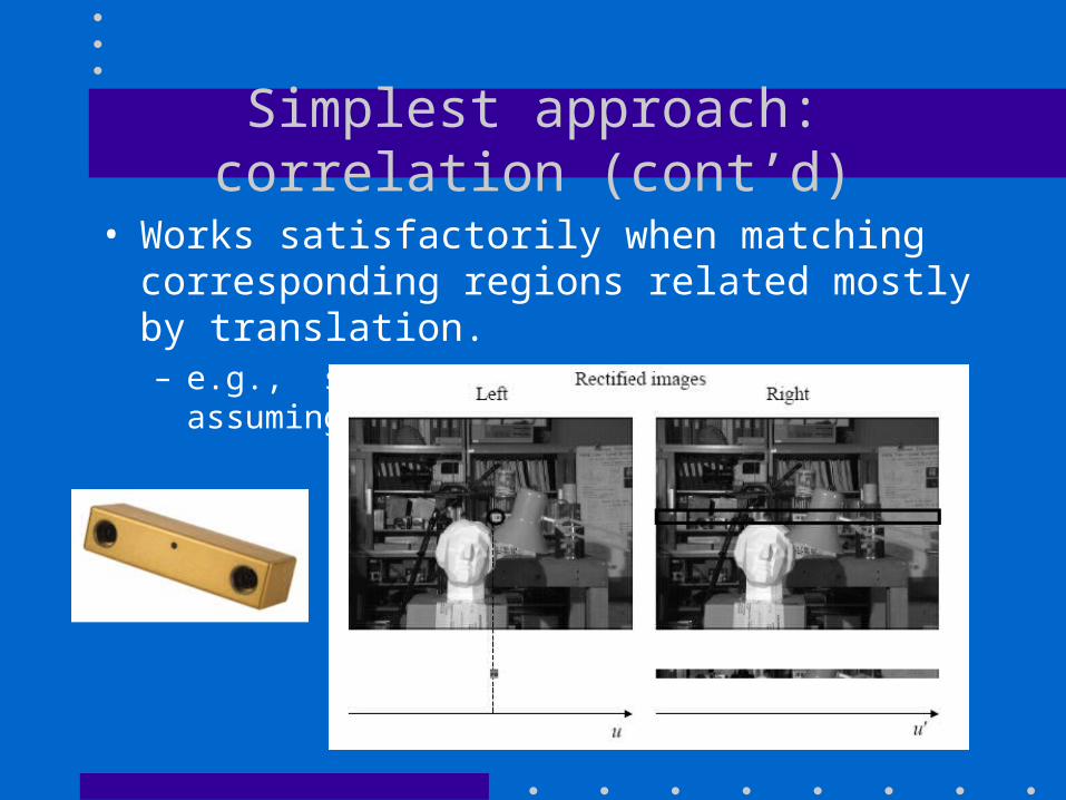
Simplest approach: correlation (cont’d)
• Works satisfactorily when matching corresponding regions related mostly by translation.– e.g., stereo pairs, video sequence assuming small camera
motion
Simplest approach: correlation (cont’d)
• Sensitive to small variations with respect to:– Location
– Pose
– Scale
– Intra-class variability
• Poorly distinctive!
• Need more powerful descriptors!

Scale Invariant Feature Transform (SIFT)
16 histograms x 8 orientations = 128 features
1. Take a 16 x16 window around interest point (i.e., at the scale detected).
2. Divide into a 4x4 grid of cells.
3. Compute histogram of image gradients in each cell (8 bins each).
Properties of SIFT
• Highly distinctive– A single feature can be correctly matched with high probability
against a large database of features from many images.
• Scale and rotation invariant.
• Partially invariant to 3D camera viewpoint– Can tolerate up to about 60 degree out of plane rotation
• Partially invariant to changes in illumination
• Can be computed fast and efficiently.

Example
http://people.csail.mit.edu/albert/ladypack/wiki/index.php/Known_implementations_of_SIFT

SIFT Computation – Steps
(1) Scale-space extrema detection– Extract scale and rotation invariant interest points (i.e., keypoints).
(2) Keypoint localization– Determine location and scale for each interest point.
– Eliminate “weak” keypoints
(3) Orientation assignment– Assign one or more orientations to each keypoint.
(4) Keypoint descriptor– Use local image gradients at the selected scale.
D. Lowe, “Distinctive Image Features from Scale-Invariant Keypoints”, International Journal of Computer Vision, 60(2):91-110, 2004.
Cited 9589 times (as of 3/7/2011)
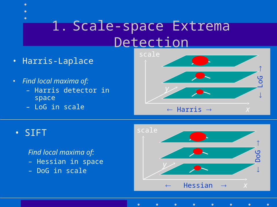
1. Scale-space Extrema Detection
• Harris-Laplace
• Find local maxima of:– Harris detector in space – LoG in scale
scale
x
y
Harris
L
oG
• SIFT
Find local maxima of:– Hessian in space – DoG in scale
scale
x
y
Hessian
D
oG

1. Scale-space Extrema Detection (cont’d)
• DoG images are grouped by octaves (i.e., doubling of σ0)• Fixed number of levels per octave
σ0
2σ0
22σ0
( , , )
( , , )* ( , )
L x y
G x y I x y
( , , )
( , , ) ( , , )
D x y
L x y k L x y
down-samplewhere

1. Scale-space Extrema Detection (cont’d)
• Images within each octave are separated by a constant factor kk
• If each octave is divided in ss intervals:
kkss=2=2 or k=2 or k=21/s1/s
k0σ0
ksσ0
k1σ0
k2σ0
…
(ks=2)

Choosing SIFT parameters
• Parameters (i.e., scales per octave, σ0 etc.) can be chosen experimentally based on keypoint (i) repeatability, (ii) localization, and (iii) matching accuracy.
• In Lowe’s paper:- Keypoints extracted from 32 real images (outdoor, faces,
aerial etc.)- Images were subjected to a wide range of transformations
(i.e., rotation, scaling, shear, change in brightness, noise).
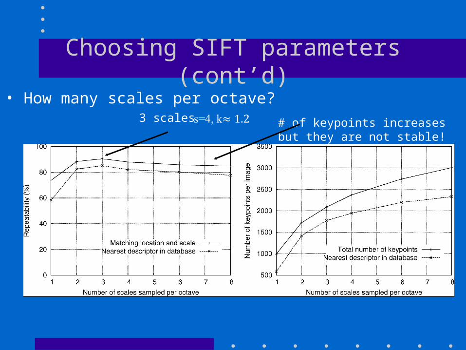
Choosing SIFT parameters (cont’d)
• How many scales per octave?3 scales # of keypoints increases
but they are not stable!

Choosing SIFT parameters (cont’d)
• Smoothing is applied to the first level of each octave.• How should we choose σ0?
σ0 =1.6
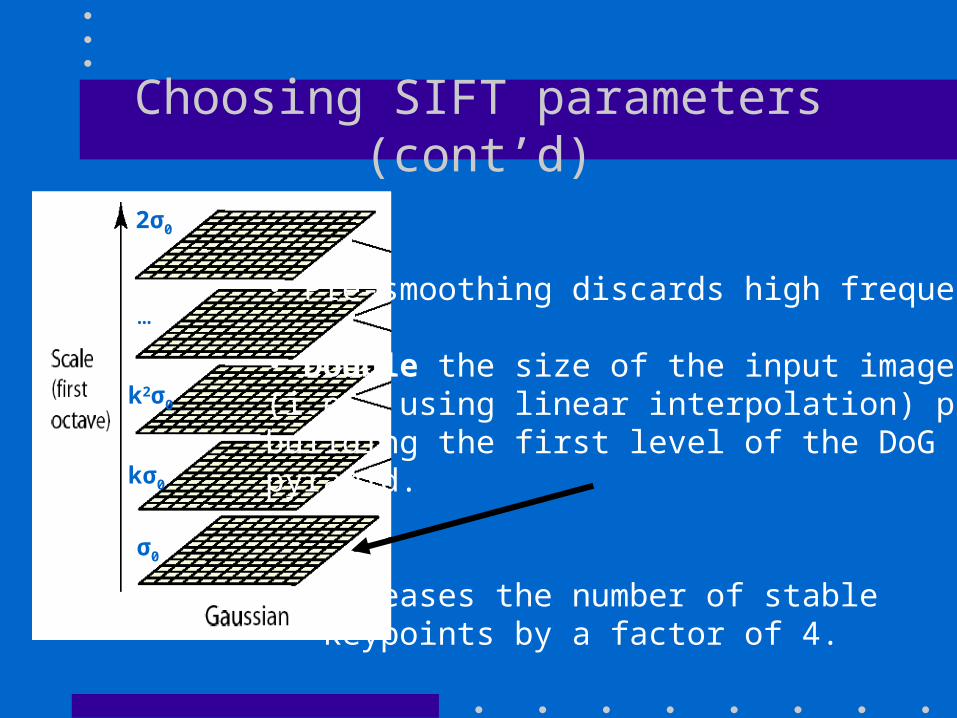
Choosing SIFT parameters (cont’d)
σ0
2σ0
kσ0
k2σ0
…• Pre-smoothing discards high frequencies.
• Double the size of the input image(i.e., using linear interpolation) prior tobuilding the first level of the DoG pyramid.
• Increases the number of stable keypoints by a factor of 4.

1. Scale-space Extrema Detection (cont’d)
• Extract local extrema (i.e., minima or maxima) in DoG pyramid.-Compare each point to its 8 neighbors at the same level, 9 neighbors in the level above, and 9 neighbors in the level below (i.e., 26 total).

2. Keypoint Localization
• Determine the location and scale of keypoints to sub-pixel and sub-scale accuracy by fitting a 3D quadratic polynomial:
i iX X X
( , , )i i iX x x y y
( , , )i i i iX x y
offset
keypointlocation
sub-pixel, sub-scale Estimated location
Substantial improvement to matching and stability!

2. Keypoint Localization
• Use Taylor expansion to locally approximate D(x,y,σ) (i.e., DoG function) and estimate Δx:
• Find the extrema of D(ΔX):
2
2
( ) ( )1( ) ( )
2
TTi i
i
D X D XD X D X
2
2
( ) ( )0i iD X D X
XX X

2. Keypoint Localization
• ΔX can be computed by solving a 3x3 linear system:
2
2
( ) ( )i iD X D XX
X X
2 2 2
2
2 2 2
2
2 2 2
2
D D D Dy x
D D D Dy
y y yx yx
DD D Dxx yx x
4
)()(
1
2
2
,11
,11
,11
,11
2
,1
,,1
2
2
,1
,1
jik
jik
jik
jik
jik
jik
jik
jik
jik
DDDD
y
D
DDDD
DDD
use finite
differences:
2 1
2
( ) ( )i iD X D XX
X X
If in any dimension, repeat.0.5X
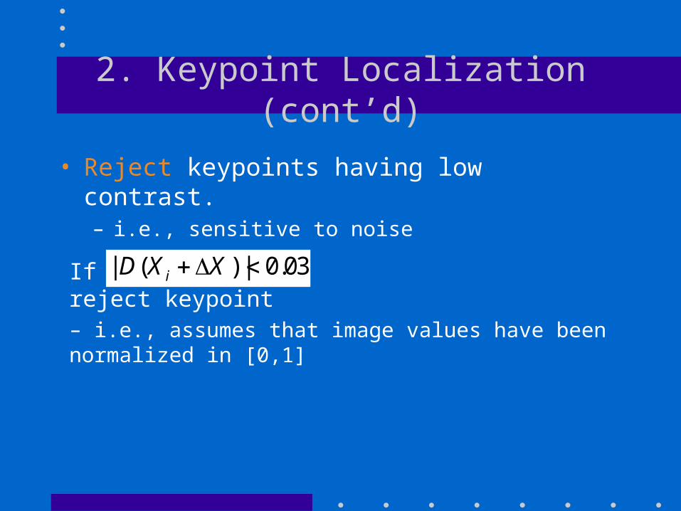
2. Keypoint Localization (cont’d)
• Reject keypoints having low contrast.– i.e., sensitive to noise
If reject keypoint– i.e., assumes that image values have been normalized in [0,1]
| ( ) | 0.03iD X X
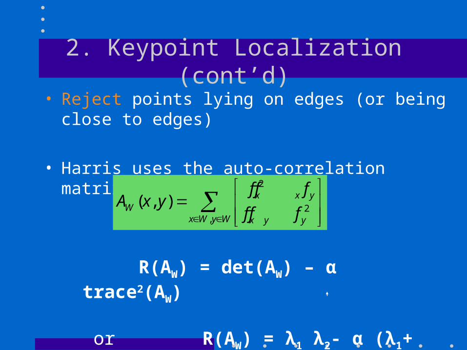
2. Keypoint Localization (cont’d)
• Reject points lying on edges (or being close to edges)
• Harris uses the auto-correlation matrix:
2
2,
( , ) x x yW
x W y W x y y
f f fA x y
f f f
R(AW) = det(AW) – α trace2(AW)
or R(AW) = λ1 λ2- α (λ1+ λ2)2

2. Keypoint Localization (cont’d)
• SIFT uses the Hessian matrix (for efficiency).– i.e., Hessian encodes principal curvatures
α: largest eigenvalue (λmax)β: smallest eigenvalue (λmin)(proportional to principal curvatures)
(SIFT uses r = 10)
(r = α/β)
Reject keypoint if:
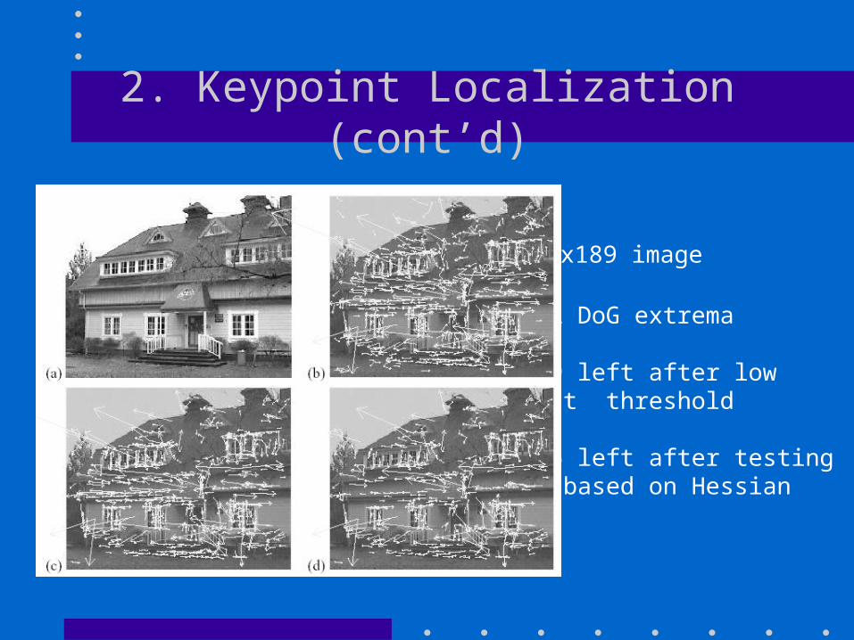
2. Keypoint Localization (cont’d)
(a) 233x189 image
(b) 832 DoG extrema
(c) 729 left after low contrast threshold
(d) 536 left after testing ratio based on Hessian

3. Orientation Assignment
• Create histogram of gradient directions, within a region around the keypoint, at selected scale:
2 2( , ) ( ( 1, ) ( 1, )) ( ( , 1) ( , 1))
( , ) tan 2(( ( , 1) ( , 1)) / ( ( 1, ) ( 1, )))
m x y L x y L x y L x y L x y
x y a L x y L x y L x y L x y
36 bins (i.e., 10o per bin)
• Histogram entries are weighted by (i) gradient magnitude and (ii) aGaussian function with σ equal to 1.5 times the scale of the keypoint.
0 2
( , , ) ( , , )* ( , )L x y G x y I x y

3. Orientation Assignment (cont’d)
• Assign canonical orientation at peak of smoothed histogram (fit parabola to better localize peak).
• In case of peaks within 80% of highest peak, multiple orientations assigned to keypoints. – About 15% of keypoints has multiple orientations assigned.
– Significantly improves stability of matching.
0 2

3. Orientation Assignment (cont’d)
• Stability of location, scale, and orientation (within 15 degrees) under noise.
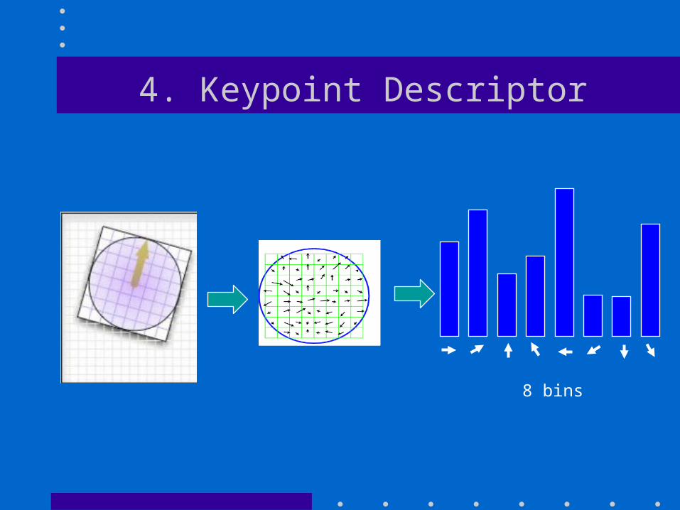
4. Keypoint Descriptor
8 bins

4. Keypoint Descriptor (cont’d)
16 histograms x 8 orientations = 128 features
1. Take a 16 x16 window around detected interest point.
2. Divide into a 4x4 grid of cells.
3. Compute histogram in each cell.
(8 bins)
4. Keypoint Descriptor (cont’d)
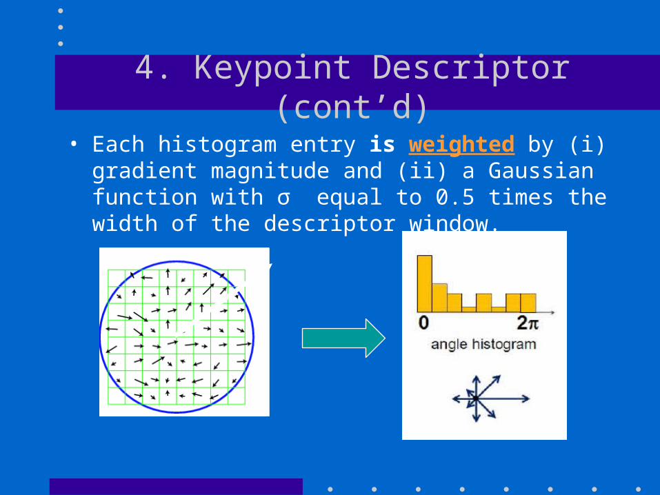
• Each histogram entry is weighted by (i) gradient magnitude and (ii) a Gaussian function with σ equal to 0.5 times the width of the descriptor window.

4. Keypoint Descriptor (cont’d)
• Partial Voting: distribute histogram entries into adjacent bins (i.e., additional robustness to shifts)– Each entry is added to all bins, multiplied by a weight of 1-d,
where d is the distance from the bin it belongs.

4. Keypoint Descriptor (cont’d)
128 features
• Descriptor depends on two main parameters:(1) number of orientations r(2) n x n array of orientation histograms
•
SIFT: r=8, n=4
rn2 features

4. Keypoint Descriptor (cont’d)• Invariance to linear illumination changes:
– Normalization to unit length is sufficient.
128 features

4. Keypoint Descriptor (cont’d)• Non-linear illumination changes:
– Saturation affects gradient magnitudes more than orientations
– Threshold entries to be no larger than 0.2 and renormalize to unit length
128 features
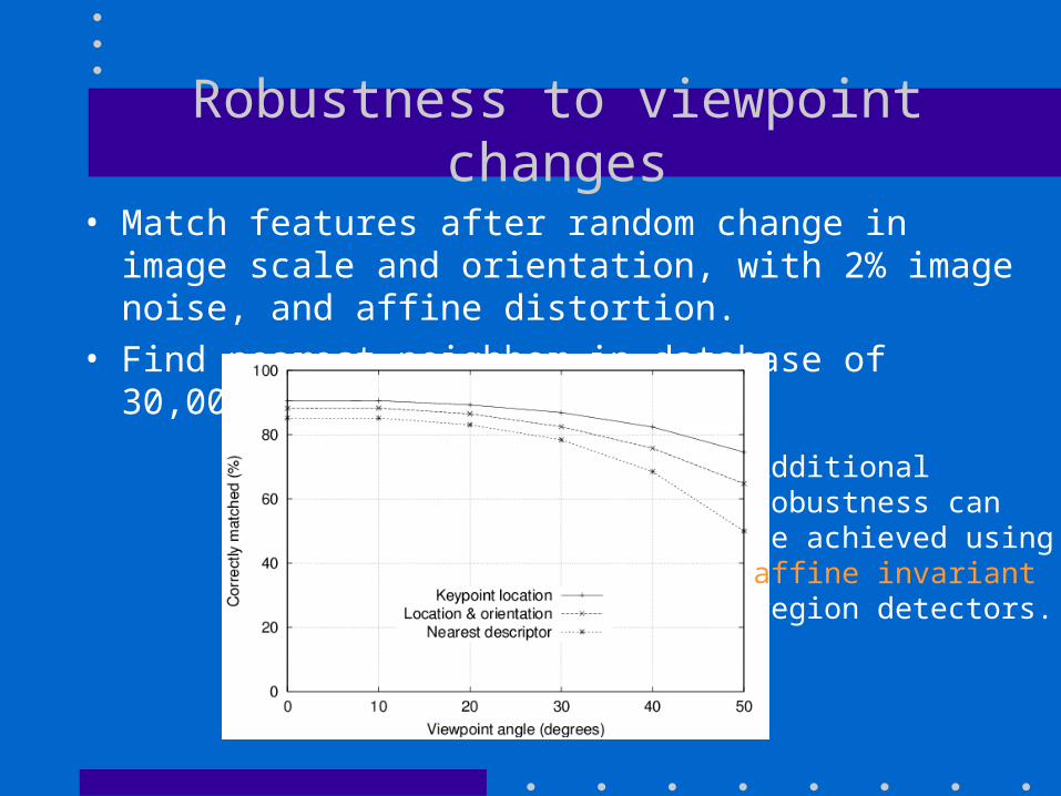
Robustness to viewpoint changes
• Match features after random change in image scale and orientation, with 2% image noise, and affine distortion.
• Find nearest neighbor in database of 30,000 features.
Additional robustness canbe achieved usingaffine invariantregion detectors.
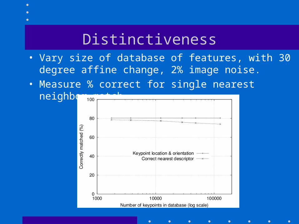
Distinctiveness• Vary size of database of features, with 30 degree affine
change, 2% image noise.
• Measure % correct for single nearest neighbor match.

Matching SIFT features
• Given a feature in I1, how to find the best match in I2?
1. Define distance function that compares two descriptors.
2. Test all the features in I2, find the one with min distance.
I1I2

Matching SIFT features (cont’d)
I1 I2
f1 f2

Matching SIFT features (cont’d)
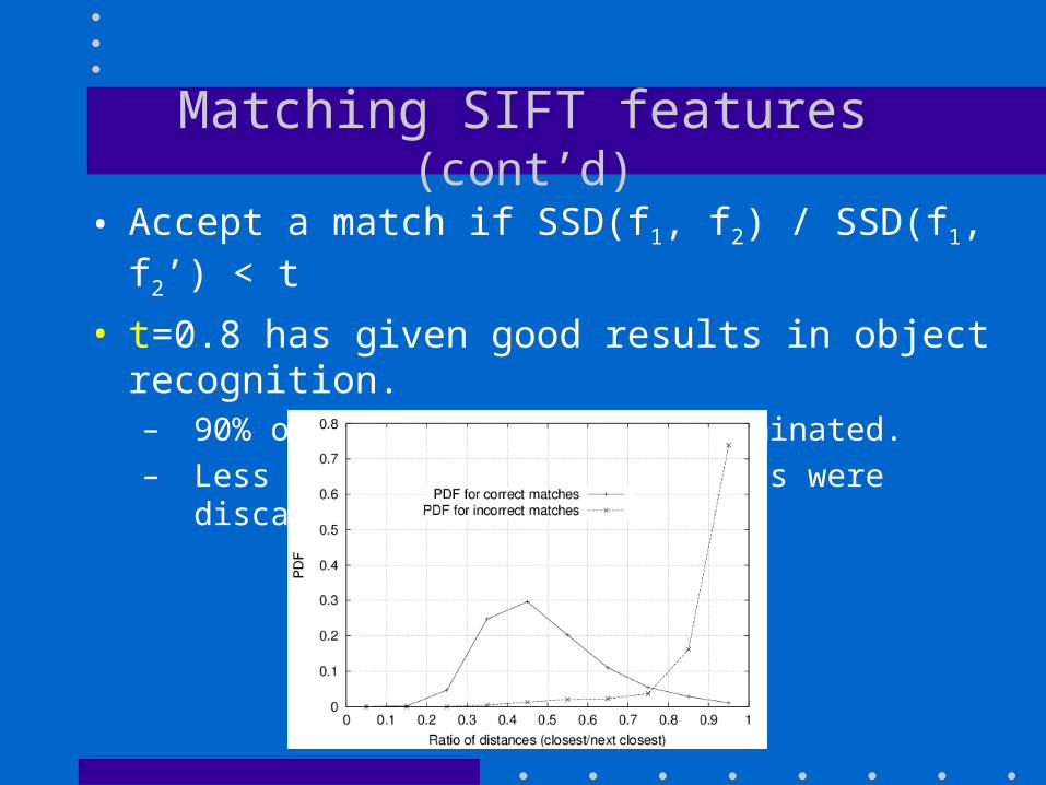
• Accept a match if SSD(f1,f2) < t • How do we choose t?

Matching SIFT features (cont’d)• A better distance measure is the following:
– SSD(f1, f2) / SSD(f1, f2’)
• f2 is best SSD match to f1 in I2
• f2’ is 2nd best SSD match to f1 in I2
I1 I2
f1 f2f2'
Matching SIFT features (cont’d)
• Accept a match if SSD(f1, f2) / SSD(f1, f2’) < t
• t=0.8 has given good results in object recognition.– 90% of false matches were eliminated.
– Less than 5% of correct matches were discarded

Matching SIFT features (cont’d)
• How to evaluate the performance of a feature matcher?
5075
200

Matching SIFT features (cont’d)
• True positives (TP) = # of detected matches that are correct
• False positives (FP) = # of detected matches that are incorrect
5075
200false match
true match
• Threshold t affects # of correct/false matches
Matching SIFT features(cont’d)
10.7
0 1FP rate
TPrate
0.1
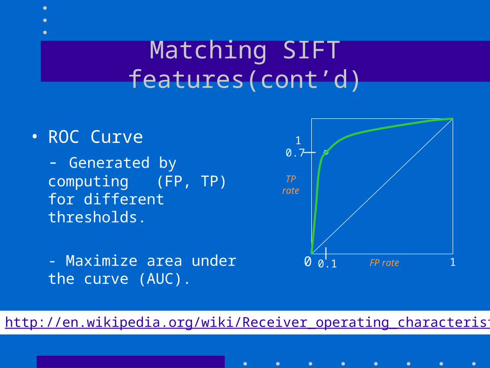
• ROC Curve
- Generated by computing (FP, TP) for different thresholds.
- Maximize area under the curve (AUC).
http://en.wikipedia.org/wiki/Receiver_operating_characteristic

Applications of SIFT
• Object recognition• Object categorization• Location recognition• Robot localization• Image retrieval• Image panoramas

Object Recognition
Object Models

Object Categorization

Location recognition

Robot Localization

Map continuously built over time
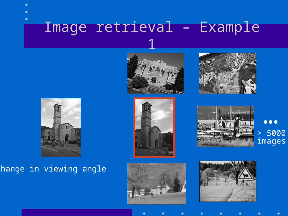
Image retrieval – Example 1
…> 5000images
change in viewing angle
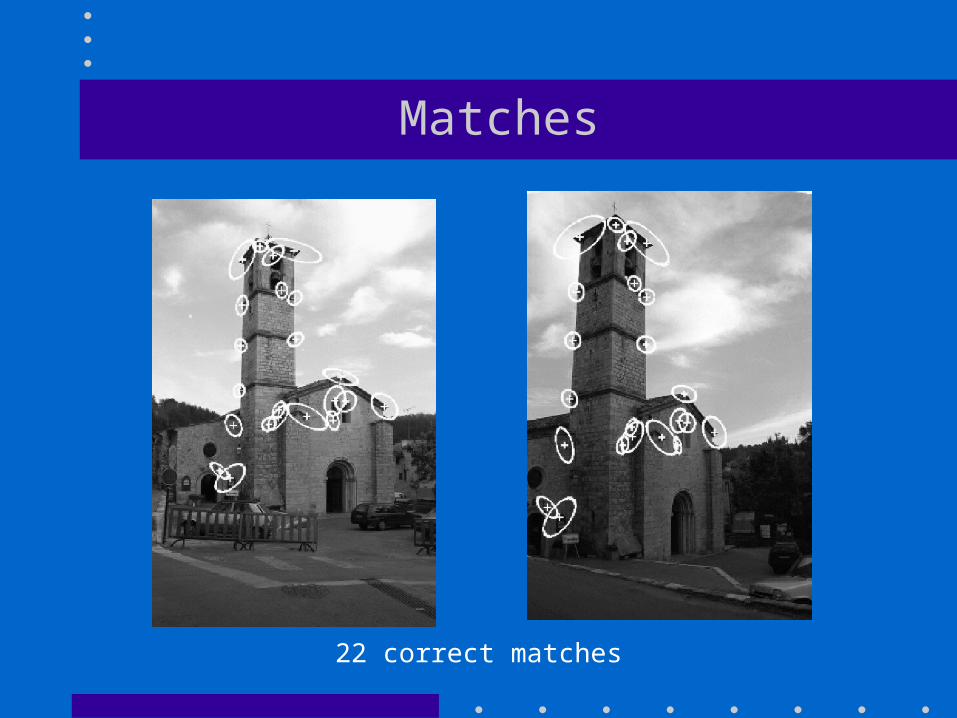
Matches
22 correct matches

Image retrieval – Example 2
…> 5000images
change in viewing angle
+ scale change

Matches
33 correct matches

Image panoramas from an unordered image set

Variations of SIFT features
• PCA-SIFT
• SURF
• GLOH

SIFT Steps - Review
(1) Scale-space extrema detection– Extract scale and rotation invariant interest points (i.e., keypoints).
(2) Keypoint localization– Determine location and scale for each interest point.
– Eliminate “weak” keypoints
(3) Orientation assignment– Assign one or more orientations to each keypoint.
(4) Keypoint descriptor– Use local image gradients at the selected scale.
D. Lowe, “Distinctive Image Features from Scale-Invariant Keypoints”, International Journal of Computer Vision, 60(2):91-110, 2004.
Cited 9589 times (as of 3/7/2011)

• Steps 1-3 are the same; Step 4 is modified.
• Take a 41 x 41 patch at the given scale, centered at the keypoint, and normalized to a canonical direction.
PCA-SIFT
Yan Ke and Rahul Sukthankar, “PCA-SIFT: A More Distinctive Representation for Local Image Descriptors”, Computer Vision and Pattern Recognition, 2004

• Instead of using weighted histograms, concatenate the horizontal and vertical gradients (39 x 39) into a long vector.
• Normalize vector to unit length.
PCA-SIFT
2 x 39 x 39 = 3042 vector

PCA-SIFT
PCA
N x 1 K x 1
'11 KxNxKxN IIA
• Reduce the dimensionality of the vector using Principal Component Analysis (PCA)– e.g., from 3042 to 36
• Some times, less discriminatory than SIFT.
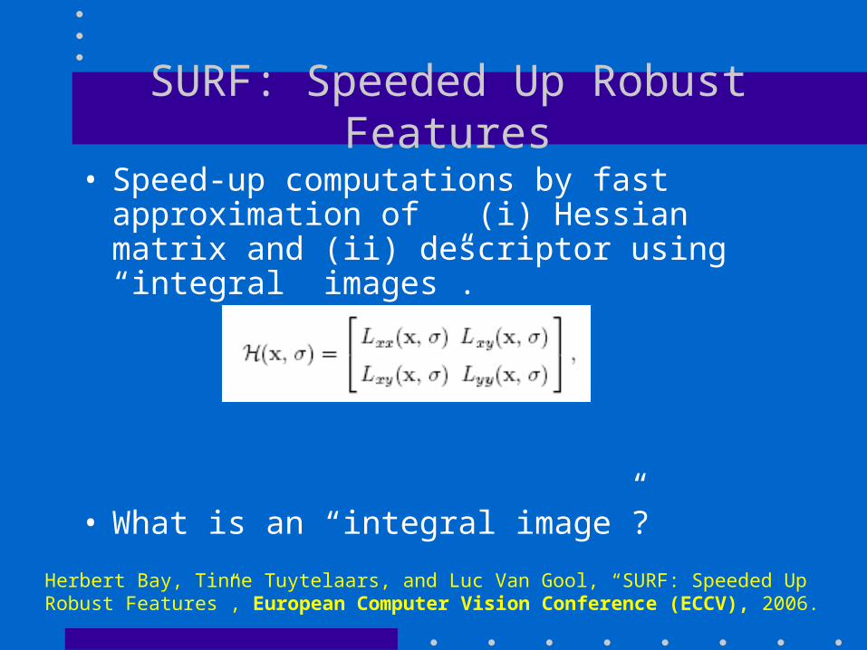
SURF: Speeded Up Robust Features
• Speed-up computations by fast approximation of (i) Hessian matrix and (ii) descriptor using “integral images”.
• What is an “integral image”?
Herbert Bay, Tinne Tuytelaars, and Luc Van Gool, “SURF: Speeded Up Robust Features”, European Computer Vision Conference (ECCV), 2006.
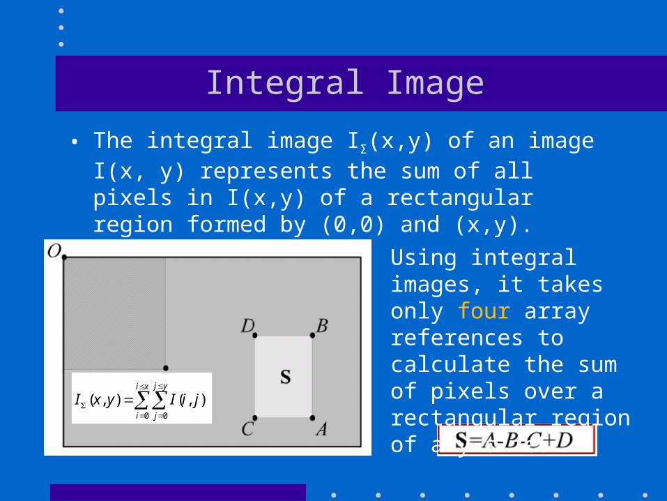
Integral Image
• The integral image IΣ(x,y) of an image I(x, y) represents the sum of all pixels in I(x,y) of a rectangular region formed by (0,0) and (x,y).
• . Using integral images, it takes only four array references to calculate the sum of pixels over a rectangular region of any size.
0 0
( , ) ( , )j yi x
i j
I x y I i j
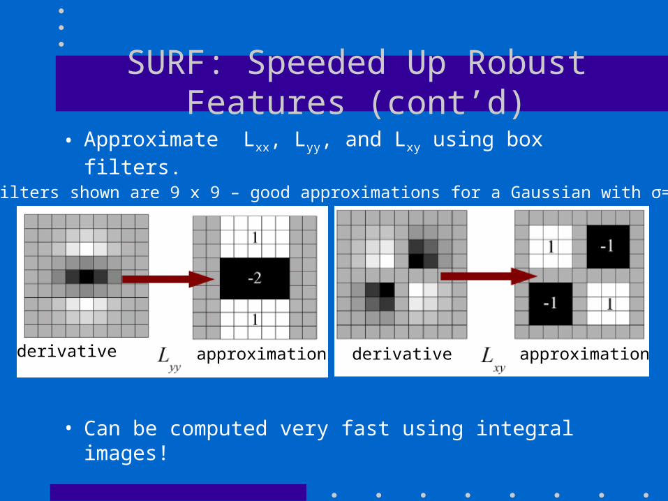
SURF: Speeded Up Robust Features (cont’d)
• Approximate Lxx, Lyy, and Lxy using box filters.
• Can be computed very fast using integral images!
(box filters shown are 9 x 9 – good approximations for a Gaussian with σ=1.2)
derivative approximation approximationderivative
SURF: Speeded Up Robust Features (cont’d)
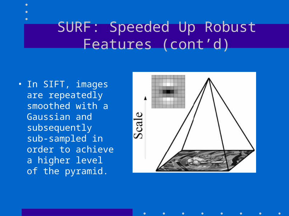
• In SIFT, images are repeatedly smoothed with a Gaussian and subsequently sub-sampled in order to achieve a higher level of the pyramid.

SURF: Speeded Up Robust Features (cont’d)
• Alternatively, we can use filters of larger size on the original image.
• Due to using integral images, filters of any size can be applied at exactly the same speed!
(see Tuytelaars’ paper for details)
SURF: Speeded Up Robust Features (cont’d)
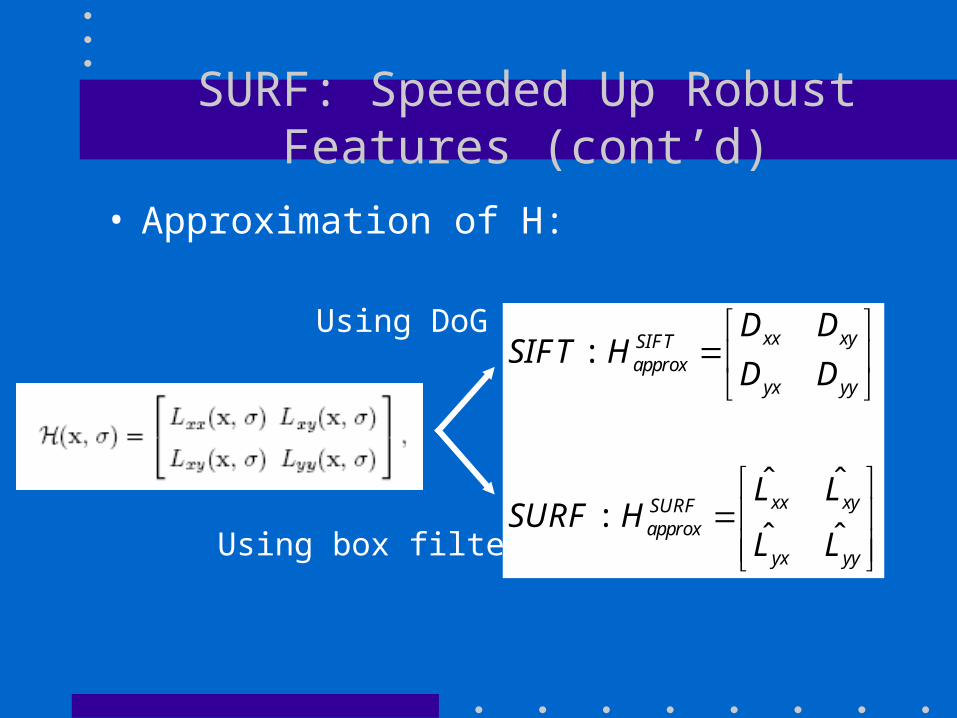
• Approximation of H:
:
ˆ ˆ:
ˆ ˆ
xx xySIFTapprox
yx yy
xx xySURFapprox
yx yy
D DSIFT H
D D
L LSURF H
L L
Using DoG
Using box filters

SURF: Speeded Up Robust Features (cont’d)
• Instead of using a different measure for selecting the location and scale of interest points (e.g., Hessian and DOG in SIFT), SURF uses the determinant of to find both.
• Determinant elements must be weighted to obtain a good approximation:
SURFapproxH
2ˆ ˆ ˆdet( ) (0.9 )SURFapprox xx yy xyH L L L

SURF: Speeded Up Robust Features (cont’d)
• Once interest points have been localized both in space and scale, the next steps are:
(1) Orientation assignment
(2) Keypoint descriptor

SURF: Speeded Up Robust Features (cont’d)
• Orientation assignment
Circular neighborhood of radius 6σ around the interest point(σ = the scale at which the point was detected)
Haar wavelets (responses weighted with Gaussian)Side length = 4σ
x response y response
Can be computed very fast using integral images!
600
angle
( , )dx dy

SURF: Speeded Up Robust Features (cont’d)
• Sum the response over each sub-region for dx and dy separately.
• To bring in information about the polarity of the intensity changes, extract the sum of absolute value of the responses too.
Feature vector size:
4 x 16 = 64
• Keypoint descriptor (square region of size 20σ)
4 x 4grid

SURF: Speeded Up Robust Features (cont’d)
• SURF-128– The sum of dx and
|dx| are computed separately for points where dy < 0 and dy >0
– Similarly for the sum of dy and |dy|
– More discriminatory!

SURF: Speeded Up Robust Features
• Has been reported to be 3 times faster than SIFT.
• Less robust to illumination and viewpoint changes compared to SIFT.
K. Mikolajczyk and C. Schmid,"A Performance Evaluation of Local Descriptors", IEEE Transactions on Pattern Analysis and Machine Intelligence, vol. 27, no. 10, pp. 1615-1630, 2005.
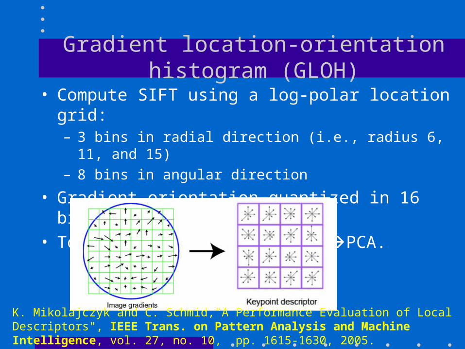
Gradient location-orientation histogram (GLOH)
• Compute SIFT using a log-polar location grid:– 3 bins in radial direction (i.e., radius 6, 11, and 15)
– 8 bins in angular direction
• Gradient orientation quantized in 16 bins.
• Total: (2x8+1)*16=272 bins PCA.
K. Mikolajczyk and C. Schmid,"A Performance Evaluation of Local Descriptors", IEEE Trans. on Pattern Analysis and Machine Intelligence, vol. 27, no. 10, pp. 1615-1630, 2005.

Shape Context
• A 3D histogram of edge point locations and orientations. – Edges are extracted by the Canny edge detector.
– Location is quantized into 9 bins (using a log-polar coordinate system).
– Orientation is quantized in 4 bins (i.e., (horizontal, vertical, and two diagonals).
• Total number of features: 4 x 9 = 36
K. Mikolajczyk and C. Schmid,"A Performance Evaluation of Local Descriptors", IEEE Transactions on Pattern Analysis and Machine Intelligence, vol. 27, no. 10, pp. 1615-1630, 2005.

Spin image
• A histogram of quantized pixel locations and intensity values.– A normalized histogram is computed for each of five rings
centered on the region.
– The intensity of a normalized patch is quantized into 10 bins.
• Total number of features: 5 x 10 = 50
K. Mikolajczyk and C. Schmid,"A Performance Evaluation of Local Descriptors", IEEE Transactions on Pattern Analysis and Machine Intelligence, vol. 27, no. 10, pp. 1615-1630, 2005.

Differential Invariants
Example: some Gaussian derivatives up to fourth order
• “Local jets” of derivatives obtained by convolving the image with Gaussian derivates.• Derivates are computed at different orientations by rotating the image patches. ( , ) ( )
( , ) ( )
( , )* ( )
( , )* ( )
( , )* ( )
( , )* ( )
x
y
xx
xy
yy
I x y G
I x y G
I x y G
I x y G
I x y G
I x y G
computeinvariants
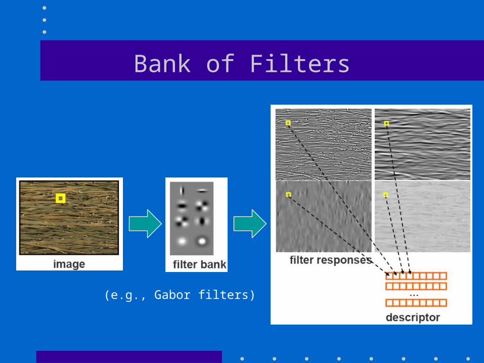
Bank of Filters
(e.g., Gabor filters)

Moment Invariants
• Moments are computed for derivatives of an image patch using:
where p and q is the order, a is the degree, and Id is the image gradient in direction d.
• Derivatives are computed in x and y directions.

Bank of Filters: Steerable Filters