interest rate scenarios · and use other means of analyzing interest rate risk. interest rate...
TRANSCRIPT

TRANSACTIONS OF SOCIETY OF ACTUARIES 1988 VOL. 40 PT 1
INTEREST RATE SCENARIOS
MERLIN F. JETTON
ABSTRACT
This paper describes several methods of creating interest rate scenarios that the actuary can use for pricing analysis or asset-liability testing. The characteristics of the methods as well as possible variations and refinements are discussed. In addition, some aids for using one method are offered.
INTRODUCTION
Recent years have witnessed the increased awareness by actuaries of the risks of changes in interest rates. The proliferation of interest-sensitive prod- ucts, such as single premium deferred annuities, has accompanied this phenomenon.
The concepts of duration and convexity are excellent tools for measuring the risks of interest rate changes. Strategies like immunization have been developed to deal with such risks. Nevertheless, the abstract nature of such concepts often makes communication difficult, especially with nonactuaries. There are various practical difficulties to implementing or using strategies like immunization. These difficulties have led many actuaries to search for and use other means of analyzing interest rate risk.
Interest rate scenarios are often used to address these hurdles. Interest rate scenarios are readily understood by nonactuaries, and basing actuarial analy- sis on scenarios facilitates communication of such analysis. Interest rate scenarios can be used to answer "what if" questions about both sides of the asset-liability equation and to develop an easily comprehended distribution of profit (or loss) results under a wide range of possibilities.
Interest rate scenarios have even appeared in the legal arena. Recently the state of New York passed a regulation that incorporates the use of scenarios to aid in formulating an actuarial opinion for the financial statements of insurers who have sold certain kinds of interest-sensitive products. It would not be surprising to see more of this type of legislation in the future, or to see more detailed scenarios.
Although interest rate scenarios have been used by more than a few ac- tuaries, there is little discussion of them in the actuarial literature. This paper addresses that dearth.
423

424 INTEREST RATE SCENARIOS
PRESET SCENARIOS
A rudimentary way of creating interest rate scenarios is to specify the rates, one by one, for as many scenarios as the creator wants to test. The span of time between different rates (for example, three months or a year), the projection period (for example, ten years), and the kind of rates (for example, 91-day Treasury bills, ten-year high-quality corporate bonds) are chosen to suit the purpose. This is an excellent way to create particular scenarios, such as the "worst case" scenario or a scenario that duplicates a particular historical period. But for many purposes this approach poses sev- eral problems:
• Are the chosen scenarios appropriate? • How many scenarios are enough? • Specifying all the desired rates can be time-consuming. For example, one might want
for each scenario all maturities up to 20 years for Treasury debt, different grades of corporate debt, and mortgage-backed securities.
• Quite often the starting point chosen for each scenario is the current or recent interest rate. In such cases, the scenarios will likely have to be created again when repeat analysis or more analysis is needed at a later date.
Specifying individual rates for particular scenarios is a method that should not be ignored, but leaves much to be desired. Therefore, we consider meth- ods that are more systematic and efficient.
The random generation of scenarios responds to all the problems listed above, particularly efficiency. The user will likely use enough scenarios to cover a wide and representative range of possibilities. Others will be less inclined to question the objectivity of the user's analysis if the scenarios are randomly generated ( " r andom" is often taken to mean "unbiased," and sometimes "object ive") . Because of these advantages, the rest of this paper is devoted to random interest rate generation.
COMMENTS ON TERMINOLOGY
The term "b i a s " is used without being well-defined. It is used in reference to properties of an interest rate generation method that may be considered undesirable, but different methods may have different kinds of biases.
Bias seems to be unavoidable with any probabilistic or stochastic method of interest rate generation. If the method is not biased in one sense, it is biased in some other sense. The term bias can, of course, have many mean- ings besides those specifically mentioned here. Also, with regard to future interest rates, one person's bias may be another person's idea of what is

INTEREST RATE SCENARIOS 425
rational. The way out of this conundrum is to choose the bias that is the least bothersome and to judge the method on the credibility of the scenarios it produces.
The words "expected" and "expectation" are used only with their strict statistical meaning: the sum of the products of possible outcomes times their respective probabilities. The words "anticipated" and "anticipation" are used when the ordinary sense of "expected" or "expectation" is meant.
BINOMIAL LATTICE [1]
The binomial lattice method of creating interest rate scenarios involves a decision tree and random decisions on which branch of the tree to follow in setting the interest rate at the next point in time. The tree or lattice can be depicted as shown in Figure 1.
FIGURE 1
BINOMIAL LATFICE METHOD FOR GENERATING INTEREST RATE SCENARIOS
1,
I3
11
Io
l_l
[-z
1.3
I_4
to t~ t2 t3 t4

426 INTEREST RATE SCENARIOS
Suppose lk = 10 + 0.5k. In other words, the interest rates are evenly spaced 0.5 percent apart with Io = 10 percent. Also, suppose that at any time tk the probabilities that the interest rate is 0.5 percent higher or lower at tk, j are both 1/2. Then a random technique (for example, a flip of a coin, or whether a random integer is even or odd) is used to determine whether the next interest rate is on the higher or lower step of the lattice.
This binomial lattice method might be criticized because the set of pos- sibilities for the next interest rate has only two members. It even precludes the possibility of the rate not changing. Such criticism is valid, but not fatal. The lattice could obviously be made trinomial, or even multinomial. Of course, the random technique would need to be modified. The binomial lattice method also becomes problematic as the number of time periods per scenario is increased. This becomes clear later in the discussion.
One might also suggest setting the interest rates at lk = 10 (1.05) k on the grounds that changes in interest rates should be proportionate to their level. The suggestion is reasonable, but one should be fully aware of the effect. Without a change in the probabilities, the change would introduce an upward bias in the interest rate scenarios created. This is because when at Ik the expected interest rate at time k+ 1 is higher than lk. For example, at 10 percent it is 1/2(10.5 percent) + l/2(9.52 percent) = 10.01 percent. This is not much bias and is insignificant over a small number of time periods, but the effect is compounded with each additional time period.
Such bias could be offset by changing the probabilities so that at interest level Ik the expected rate for the next time period equals lk. Changing the probabilities, of course, invites the criticism that the lattice is biased in the sense that the next interest rate at any time is anticipated to decrease more often than increase.
YIELD CURVE JUMPING [3]
A third method is a probabilistic approach to scenario generation. The technique involves specifying a set of interest rate curves (for example, A- rated corporate bonds) and the probabilities of jumping from one curve to any other in a fixed interval of time (for example, one year). Then, using a random technique and the curves and probabilities specified, one can gen- erate as many scenarios for as long a projection period as desired.
A fairly simple example illustrates the method. Figure 2 shows a limited range of possible yield curves.

INTEREST RATE SCENARIOS
FIGURE 2
YIELD CURVE JUMPING METHOD OF SCENARIO GENERATION
427
e -
/
Curve
Years to M a t u r i t y
The probabilities of moving from any one curve in Figure 2 to any other curve in Figure 2 are given below:
From Curve
Pll P21 P31
P,I
To Curve
2 3 4
Pl2 P13 -- P~ . . . . . .
5 6 7
M
PI?
P77
The sum of the probabilities in each row is 100 percent. Some individual probabilities could, of course, be zero. Interest rate scenarios are generated by using some random choice technique, for example, random numbers that are "mapped" to the probabilities in the table.
The random technique can be visualized as a roulette wheel, or as a spinner for a board game, with 100 possible outcomes. For example, when at curve 3, the 100 possible outcomes are P3~ l ' s , P32 2's, P33 3's, and so on. A spin

428 INTEREST RATE SCENARIOS
of the wheel or spinner determines the curve number at the next point in time in the interest rate scenario. Subsequent spins determine the curve for each subsequent point in time in the scenario, and this technique is used for as many scenarios as desired.
When using this method, as well as any other, one should be aware of the possible biases. For example, if the probabilities in the fourth row of the table are not normally distributed around curve 4, there will be a bias, at least in some sense. The expectation could still be upward or downward and would depend on the interest rates on the curves. Of course, this ex- pectation could vary depending on which curve one is on. When on either the top or bottom curve of Figure 2, it is impossible to eliminate bias in the sense of equal probabilities of rates going up or down.
FIRST STOCHASTIC MODEL
Another way to generate interest rates is to use a recursive algebraic formula in which the interest rate for the next period is determined from the current period interest rate, a random variable, and one or more parameters or constraints. The formula that comes readily to mind is the following:
I,+, = I, ( I + Z x V F )
where I, is the current interest rate; I,+ ~ is the interest rate one period later; Z is a random variable that is normally distributed with a mean of 0 and standard deviation of 1 (Appendix A describes means of developing these random variables, which can be easily programmed on a computer); and VF is a volatility factor appropriate for the time period from t to t + 1 and for the particular interest rate (for example, the one-year Treasury rate or the ten-year Treasury rate).
This model has an advantage over the previous models in that the number of possible outcomes is limited only by the number of possible Z's. It also invites looking at actual historical interest rates to set the volatility factor.
Not much is said about this model because the next model described is quite similar, yet better than this one. The above formula, without a con- straint added, would have the flaw that it could produce a zero or negative interest rate. All it would take is for Z x VF to be less than or equal to - 1. Therefore, the formula should only be used with a lower bound on I1,+ t or Z.

INTEREST RATE SCENARIOS 429
SECOND STOCHASTIC MODEL
D e v e l o p m e n t
Let us alter the previous model by assuming instead that In [(I + A / ) ÷ / ] is normally distributed. Now we can generate interest rates by using the following formula:
I . . l = l ,e z×vr
where the symbols have the same meaning as in the previous formula. This author has found that changes in historical interest rates are approx-
imately normally distributed, whether measured simply or logarithmically. Suppose we have a history of one-year Treasury rates over many years at
our disposal and find that the standard deviation over one-year periods of In [(•+ A I ) + / ] equals 0.27. Further, suppose we set V F = 0.27 in the above formula and generate scenarios.
Unfortunately, this approach only a p p e a r s to produce interest rates con- sistent with history. Actually, the distribution of the randomly generated interest rates is much more varied than the historical rates over multiple time periods, even though the volatility over one-year periods is fine. This is clear from the following formula:
I , . , , = I, e vv~zj ,z2 . . . . . . z ,) .
For example, suppose I, = 8 percent, and E~=~ Zt. = 5. Then I,+,, = 30.86 percent.
How might the model be changed to avoid such unrealistic rates? Three possibilities are:
1. Lower the volatility factor. 2. Put bounds on how high or how low the rates can go. 3. Both of the above. The first solution may be appropriate if short-term rate fluctuations are
not important to the application; however, they often are. The second so- lution is more practical; it may even be suitable for the application. But it will cause the interest rates in a number of scenarios to " s t i ck" at or near the upper or lower bound. Also, it invites the criticism of a bias against rates outside of the bounds. Interest rates may also "s t i ck" with the yield curve jumping model, unless the probabilities of moving from the extreme curves are very skewed.

430 I N T E R E S T R A T E S C E N A R I O S
Comparison with Prior Models
Suppose we were to construct a series of lattices, L3, Ls, L 7 , - • • , the subscript indicating the number of branches at each node on the lattice. Further suppose that for each lattice the interest rates were geometrically spaced and the probabilities were "normally distributed" as much as pos- sible. Then the limit of the series would be the lognormal model just de- scribed (with no bounds).
We saw earlier that a lattice with the interest rates geometrically spaced resulted in an expected interest rate at time t + 1 higher than I,, but that this bias could be removed by changing the probabilities. This becomes difficult as the number of branches at each node is increased, but would be practical with this model. It could be done by shifting the mean of the variable Z downward from zero to a small negative number.
Let us assume that the interest rates on the curves in the yield curve jumping model are geometrically spaced and that the probabilities at each curve are "normally distributed" as much as possible. That would be anal- ogous to this second stochastic model with upper and lower bounds.
T H I R D S T O C H A S T I C M O D E L
The third stochastic model addresses some of the shortcomings of the last model and extends it to generate yield curves, rather than just one kind of interest rate. The model assumes a starting one-year Treasury rate, TI(0), and a starting twenty-year Treasury rate, 7"20(0). The future interest rates are generated in steps: first the one-year rate, then the twenty-year rate, and finally the intermediate rates.
One-Year Treasury Rate
To maintain the short-run volatility shown by history yet temper the long- run volatility, this model incorporates a mean-reverting formula, rather than imposing an upper and lower bound. The one-year Treasury rate one year later, Tl(t+ 1), is calculated as:
T , ( t+ l ) = [T,(t) + f(t)]e z×VF

INTEREST RATE SCENARIOS 431
where f(t) = minimum {.015[T~(00) - T~(t)]3; .5[T~(®) - T,(/)]}
if T~(t) < TI(®) = maximum {.015[/'1(00) - T,(t)]3; .5[T1(®) - T~(t)]}
if T~(t) >_ T~(®); T~(®) is a parameter signifying the " long-run" T~; and Z and VF are defined as in the last model. The function f(t) defined above is not derived from a detailed analysis of
historical data. It does, however, reflect a commonly held view about real- world interest rates. Its varying effect is consistent with the economic law of supply and demand. Clearly, it has very little effect if the difference between T~(t) and TI(Q0) is small and a greater effect as the difference in- creases. When current interest rates are above or below what interested parties perceive to be "normal , " then market forces exert their effect to bring them back into line. And the further from "normal" rates are, the stronger the forces.
A mean reverting function might be criticized from the standpoint that at any given time no one really knows where future interest rates will be; yet the model says that the anticipated rate, T~(t) + f(t), is toward T~(~). The criticism has a certain amount of validity, but perhaps the only alternative is a less realistic model.
One more point is worth discussing. Where does one set Tj(~)? It would typically be set at T1(0), but that is not obligatory. One may set it above or below to effect an upward or downward bias on the interest rate scenarios, if it is thought that the starting interest rates are " l o w " or " h i g h . "
Let us now compare this model with the prior one. The prior model, with the upper and lower bounds, also has a sort of market force as just described. But its behavior is quite different. It has no effect until the interest rate is far from normal. It does not allow the interest rate to go past the bound. It does not pull the interest rate back toward normal.
Twenty-Year Treasury Rate
We noted that the one-year Treasury rate is a function of its anticipated rate and a random term. A similar approach is taken for the twenty-year Treasury rate. The formula is as follows:
T2o(t+l) = [axT~( t+l ) + b] + Z(r2o.

432 I N T E R E S T R A T E S C E N A R I O S
The variable Z is random, normally distributed with a mean of 0 and a standard deviation of 1. Theterm cr2o is the standard deviation of the spreads, presumably derived from historical data, between one-year and twenty-year Treasury rates. Suggested values for a, b, and e2o are given in Appendix B.
The bracketed part of the formula is the anticipated rate and recognizes an important constraint on the " r a n d o m " generation of simultaneous interest rates: There must be a reasonable relationship between any one rate and another.
The above formula, using the values suggested in Appendix B, is graph- ically depicted in Figure 3. The solid curve shows the anticipated twenty- year rate. The broken curves above and below the solid curve indicate the anticipated twenty-year rate _+ Cr2o. Thus, about 68 percent of the time T2o(t + 1) would be anticipated to fall between the broken curves. Points on the graph that are below the 45-degree line would give inverted yield curves.
FIGURE 3
TWENTY-YEAR TREASURY RATE AS A FUNCTION OF THE ONE-YEAR TREASURY RATE AND A RANDOM TERM (VALUES FROM APPENDIX B)
14 r
12
/ /
/ /
10 O
8
6
o
4
f f / / / /
/ / / / j
/
/
,,9" f
f
j f
/
4 6 8 10 12 14 One-Year Treasury Rate
16

INTEREST RATE SCENARIOS 433
A historical graph of twenty-year rates versus one-year rates would not look as simple as the one in Figure 3. For example:
• The middle curve, representing average twenty-year rates, would be bumpier. • The "band" would be a little wider in the middle and narrower at the high end,
probably because of the high number of occurrences of interest rates in the midrange and low number of occurrences of interest rates above 12 percent.
History cannot be formulated so easily. But Figure 3, and hence the values in Appendix B, will give good results for almost any practical application.
Other Treasury Rates
Linear combinations of Tl(t) and T2o(t + 1) for the intermediate maturities would probably give satisfactory results for many practical applications. The formula could be expressed as:
T,,(t+l) = [Wl(m) x TI(t+I)] + [W2o(m) x Tzo(t+l)] (2_<m<19)
in which W1 and W2o are weights for the one-year and twenty-year rates. Alternatively, one could set Tm(t + 1) for two to four key values of m, for example, m = 2, 5, 7, and 10, and interpolate to find the remaining Tm(t + 1).
This approach makes no attempt to simulate the multitude of shapes that the Treasury yield curve may have in the real world. The user is invited to search for a formula or formulas, or even add one or more random elements, to more closely represent the real world.
The Starting Curve
If one were to select a starting curve from the real world, only by pure coincidence would it match the curve that would result from starting with TI(0) and then calculating 7,,(0) (m > 1) with Z = 0, using the above formulas. Rather, the real-world starting curve would be to some degree inconsistent with the later randomly generated curves. One could ignore the inconsistency, bend the real-world curve to fit the model, or adjust the formulas. The last option might involve minor adjustments initially that later diminish and grade into the unadjusted formulas over time. For example, one might use two different formulas for deriving the anticipated twenty-year rate from the one-year rate. The first formula might be for t = 0, the second for t -> 5, and a weighted average of the two formulas for t = 1 to 4.

434 INTEREST RATE SCENARIOS
MULTIPLE CURVES
The last model described a method of generating yield curves for Treasury rates. What if the user also wanted other simultaneously occurring interest rates, such as corporate debt or mortgages?
Interest rates for other kinds of debt can be determined by simple formulas using the Treasury rates for the same maturity. Two possibilities readily come to mind. The first is an addition to the Treasury curve, that is, a so- called quality spread. The second is a multiple of the Treasury rate, which would give a "quali ty spread" that varies with the level of the Treasury rate. The latter is probably more realistic. Either method would probably yield satisfactory results for any practical application. Perhaps time studies of quality spreads have been made and published by someone, but the author is not aware of any.
Whichever formula is chosen, all the following pertain:
• Quality spreads vary significantly with the number of years to maturity. • If the application does not model defaults, then the calculation of the interest rates
should incorporate a credit risk deduction to indirectly allow for defaults. • In the real world, quality spreads are dismayingly volatile. One might specify quality
spreads that are higher (or lower) than normal at the starting poin! for each scenario and grade into more normal spreads later in the scenario. However, doing so would build in a bias.
The volatility of quality spreads in the real world might suggest two kinds of refinements:
• Quality spreads that vary with the economic cycle, narrowing during good times and widening during bad times, however the user might determine those times by interest rates.
• Adding a random element to the calculation of the interest rates for the other kinds of debt.
However, the effort that would be required to measure, program, test, and monitor the refinements probably would far exceed the benefits derived from the refinements.
CONCLUSION
This paper has described methods of creating interest rate scenarios, which are a valuable tool for analyzing interest rate risk and facilitate communi- cation of analysis of such risk. The methods described are skeletal in form. The use of variations, combinations, refinements, and different parameters is encouraged, with one precaution: Analyze the practical results. Are they

INTEREST RATE SCENARIOS 435
reasonable in relation to historical rates? What is the short-run volatility? The long-run volatility? How frequent are the highs and lows? How high and low are they?
The thrust of the first and second stochastic model was toward randomly generated interest rates that are closer to historical reality. This goal was pursued more vigorously with the third stochastic model. Without a com- prehensive theory of the behavior of interest rates, such a pursuit lacks scientific precision. That does not mean that the pursuit should not be un- dertaken. The more realistic we actuaries can make our scenarios, the more credible will be the results.
The use of interest rate scenarios by actuaries is of fairly recent origin, as is the systematic development of such scenarios. The methods described in this paper eventually may be viewed as unsophisticated. But this author hopes that this paper will contribute to the evolution.
How might the model be further improved? Two ideas that seem worthy of consideration are the cyclical nature of interest rates and changes in in- terest rates between different eras, such as before and after October 1979.
REFERENCES
1. CLANCY, R.P. "Options on Bonds and Applications to Product Pricing," TSA XXXVII (1985): 97-151.
2. LEWIS, T.G. Distribution Sampling for Computer Simulation. Lexington, Mass.: Lexington Books, 1975.
3. TULJN, S.B. "Actuarial Opinions on Asset-Liability Matching," RSA 11, no. 4B (1985): 2325-27.
APPENDIX A
The stochastic models require random variables, Z, which are normally distributed with a mean of 0 (Ix = 0) and a standard deviation of 1 (o- = 1). Most statistics textbooks tell us that a normal distribution closely ap- proximates a binomial distribution if certain conditions are met. This fact is used because binomial distributions are easily done on a computer, which will give random numbers.
Let X1, X2, . . . , XN be a sequence of l ' s and O's each indicating a "success" or "fa i lure" where the probability of a success is 1/2 (P = 1/2). Let X equal the sum of the sequence. If N, the number of trials, is sufficiently large, then Ix = NP, tr = ~ / N P ( 1 - P ) , and (X - Ix) + o is normally distributed.

436 INTEREST RATE SCENARIOS
The sequence of l ' s and O's can be produced on a computer by random selection on two possibilities, for example, determining whether a random integer from a range of integers (the range even-numbered or very large) is even or odd. Therefore, it takes little more than N random numbers to produce Z = (X - 0.5N) + 0.25N, which is normally distributed with p~ = 0 and ~ = 1. N = 30 is suggested as a minimum. It is reasonable to discard Z if IZ[ > 3.
There are more esoteric and efficient methods for generating values of Z that are normally distributed with ix = 0 and cr = 1. For example, there is the Box-Muller method [2]. Let U~ and U2 be random numbers, both from the unit interval (0,1). Then two random numbers Z, and Z2 can be calculated a s :
Z, = ( - 2 In UI) u2 cos(2rrU2)
Z2 = ( - 2 In U~) 'tz sin(2rrU2).
APPENDIX B
The volatility factors in all stochastic models and the cr2o in the third stochastic model are important. An effort was made in both models to allow parameters based on historical data. Of course, the numerical value implied by the data will vary with the period of history studied.
For the second stochastic model (the lognormal formula) a reasonable value for the volatility factor to model one-year Treasury rates at one-year intervals is about 0.27.
For the third stochastic model a reasonable value for the volatility factor to model one-year Treasury rates at one-year intervals is about 0.23. It is lower than the 0.27 because the mean-reverting function adds some short- run volatility.
Suggested parameters for calculating the twenty-year Treasury rate are as follow:
a = 0.8 b = 2.5 if T1 < 10% a = 0.6 b = 4.5 ifT~ > 10% cr2o = 0.2 + 0.1T'zo if T'zo -< 10% ] T'zo is the
Crzo = 1.2 if T'zo > 10% J anticipated rate.

INTEREST RATE SCENARIOS 437
Suggested weights for calculating the in-between Treasury rates are as follow:
m Wl(m ) W2o(m )
2 0.64 0.36 5 0.39 0.61 7 0.24 0.76
10 0.16 0.84


DISCUSSION OF PRECEDING PAPER
STEPHEN J. STROMMEN:
Mr. Jetton has provided an excellent and thorough introduction to the topic of interest rate scenarios. His paper is a welcome addition to the actuarial literature.
This discussion describes two possible modifications to the third stochastic model described in the paper. These modifications have proven useful in practice, and one of them is supported by historical data. Throughout this discussion, the notation follows that used by Mr. Jetton in describing his third stochastic model.
A Different Mean-Reverting Formula One of the assumptions in the third stochastic model is the long-run normal
interest rate on one-year Treasuries TI(~). When interest rates are higher than TI(®), they tend to fall, and when they are lower than T~(~), they tend to rise. This is accomplished in the model by using a function, f(t), which is negative when interest rates are higher than Tt(®) and positive when interest rates are lower than TI(®). The assumption is that next year's interest rate, Tj(t+ 1), is randomly distributed around T~(t)+f(t).
The difficulty with this procedure is in choosing an appropriate value for T](®). As Mr. Jetton noted, if the chosen value is different from T~(0), an upward or downward bias is built into every randomly generated scenario. One could consider that to be undesirable, because it is very difficult to build a strong argument for any particular choice of T~(~).
An alternative approach involves an assumption that there is a range of normal values of T~(®) rather than a single value. For example, assume that TI(®) = T~(t) as long as T~(t) lies between 4 percent and10 percent. T](~) is then never lower than 4 percent nor higher than 10 percent. Mr. Jetton's formulas for f(t) can still be used, but this change in T](®) results in f(t) being zero whenever the one-year Treasury rate lies between 4 percent and 10 percent.
This approach eliminates the need to choose a single normal level for interest rates and replaces it with the need to choose a normal range. Aside from the effect on the resulting scenarios, the use of a range of normal values can make it easier to get agreement from a large number of people that a given assumption is realistic. It also makes it less likely that the assumption will need to change from time to time.
439

440 INTEREST RATE SCENARIOS
A Different Approach to the Slope o f the Yield Curve
Throughout the paper, Mr. Jetton tacitly assumes that the slope of the yield curve is directly connected to the level of interest rates. The higher the interest rates, the smaller the slope of the yield curve.
~This shows up in Figure 2 for the "yield curve jumping" method. In Figure 2, all the yield curves for the high interest rates are inverted, while all of those for low interest rates are positively sloping.
It shows up again in Figure 3 for the third stochastic model. In Figure 3 the difference between the one-year Treasury yield and the 20-year yield is randomly distributed around a figure that gets smaller as interest rates rise. By using this model, it is very unlikely that one could randomly generate a positively sloping yield curve when interest rates are at 14 percent, nor could one generate an inverted yield curve when interest rates are at 6 percent.
An alternative approach to the slope of the yield curve is based on a fundamentally different assumption:
The slope of the yield curve depends more on whether interest rates previously went up or down than on the current absolute level of interest rates.
This assumption can be implemented by using the procedure described below. In addition, it will be shown to have some support from historical data.
To aid in the discussion, let us define the "s lope" of the yield curve as:
s(t) = [T2o(t) T,(t)] / T,(t)
so that
T2o(t ) = Tt(t).[1 + S(t)].
Under this definition, the slope is zero when the yield curve is flat. Let us also assume that there is some "normal" value of S(t); call it S(®).
To implement our assumption, let us make S(t) follow a recursive rule. In particular,
S(t + 1) = (1 - a) " S(~) + a.S(t) + b.[T,(t + 1) -T , ( t ) ] / r , ( t ) [1]
In words, this means that next year's yield curve slope is equal to a weighted average of this year's slope and the normal slope, plus a shock factor based on the change in interest rates. Assuming that b is less than zero, any sudden increase in interest rates tends to decrease the slope (perhaps creating an inverted yield curve), but if interest rates remain level thereafter, the slope returns to normal.

D I S C U S S I O N 4 4 1
It can be useful to put limits on the projected value of S(t); one might assume that it must fall between - 0 . 2 5 and + 0.50. This prevents the slope from getting unreasonable in a scenario in which interest rates move in the same direction in sizable amounts for a few years in a row.
Given these definitions, historical data can be used to arrive at reasonable values for the constants S(~), b, and a. If we make the transformation c = S(®)-(1 - a), we can express [1] in a form suitable for a linear regression on two independent variables, as shown in [2] below.
[2] Y = c + aX~ + bX2
where Y = S(t + 1) x, : s(t) Xz = [T~(t + 1) - T,(t)]/T~(t)
Use of historical data on government securities for the period 1960-84 leads to the following regression results:
Parameter Estimate
c 0+064 a 0.718 b -0.587
S(z) = cl(I-a} 0.227 R - squared 0.934
Using these values, the fit between actual and projected slopes is quite good, as is shown in Chart 1 (the data are given in Table 1). In Chart 1, the estimated slope S(t + 1) is calculated from the previous estimated value of S(t) rather than the previous actual value. The fact that the estimated slopes follow the actual ones so closely indicates that the recursive rule works quite well when using parameters estimated from the regression.
When using this alternative approach to the slope of the yield curve, the procedure generating an interest rate scenario for Treasury rates is as follows:
1. Calculate the one-year Treasury rates Tt(t ) for all future years. 2. Calculate the yield curve slope S(t) recursively for each future year, starting with
the current actual slope. 3. Calculate the 20-year Treasury rates from the one-year rates and the slopes: T2o(t)
= T,(t)[1 + S(t)]. 4. Calculate other points on each year's yield curve in the manner suggested by Mr.
Jetton.

Chart 1
Yield Curve Slope 1960-[14
0.4
0.3'
0.2
0"10
-0.1 i X
- ' 0 . 7 ' ~ I I I I I I I I ! I I I I I I I I I I I ! I I I 1
1960 1970 1980
, n ¢ 5 . ~ 1
JI,
[ntirr~t~l
TABLE 1
S i c ~e
Y e a r A c t u a l E s t i m a t e d
1960 1961 1962 1963 1964 1965 1966 1967 1968 1969 1970 1971 1972 1973 1974 1975 1976 1977 1978 1979 1980 1981 1982 1983 1984
0.1634 0.3495 0.3180 0.2280 0.1000 0.0393
-0 .0781 0.0335
-0 .0253 -0 .1007 -0 .0369
0.2290 0.1885
-0 .0373 -0 .0365
0.2090 0.3277 0.2828 0.0268
- 0.1233 -0 .0646 -0 .0706
0.0540 0.1901 0.1438
0.1571 0.2859 0.2367 0.1877 0.1078 0.0997
-0 .0159 0.0927 0.0358
-0 .0597 0.0127 0.2529 0.2467
- 0.0427 - 0.0469
0.1430 0.2310 0.2278 0.0042
-0 .1004 -0 .0933 -0 .1324
0.0618 0.2470 0.1515

DISCUSSION 4 4 3
Random numbers are only used in Step 1. The rest of the procedure is completely deterministic.
Closing Comment
This discussion has provided two possible modifications to the third sto- chastic model presented by Mr. Jetton. Given the current state of actuarial knowledge and practice in this area, it is not possible to say whether they represent a definite improvement. The key, as Mr. Jetton pointed out, is to "Analyze the results!"
JEFFREY M." GURSKI:
Mr. Jetton should be commended for his valuable ground-breaking efforts. The projection of plausible yield curves is an essential and timely topic for many actuaries who need to model their business over various future scen- arios. This discussion presents an alternative to Mr. Jetton's third stochastic model, as well as some comments on the author's version. The alternative version involves first the projection of the ten-year rate in a manner similar to the author's projection of the one-year rate. Then conditional distributions are used to generate movements of the one- and thirty-year rates in a manner that correlates them to the ten-year move.
I. ANALYSIS OF HISTORICAL DATA--RESULTING ASSUMPTIONS
Historical Data
Salomon Brothers" Analytical Record of Yields and Yield Spreads pro- vides an historical data base of month-to-month Treasury yields (i (2) basis) for various maturities back to 1954. This data base was used to:
(1) Test whether the natural logarithms of the changes in yields are indeed normally distributed
(2) Determine what are reasonable levels and slopes of the yield curve (3) Study the volatility patterns of the one-, ten- and thirty-year yields (4) Study the correlation between the movements of the one- and thirty-year yields to
those of the ten-year.
It could be argued, especially in today's rapidly changing financial world, that history should not be used to predict future results. However, we are not predicting any one future. Rather, we are trying to determine a set of plausible futures. Actual historical results will likely provide more reliable guidelines for this purpose than our intuition.

444 INTEREST RATE SCENARIOS
Definition of Random Variables Because the alternative version involves the projection of the one-, ten-
and thirty-year Treasury yields, we focus only on these. The rest of the curve is filled in by using an interpolation that is detailed in Appendix B. Three rates are projected rather than-two in order to better model the various shapes that the yield curve can take on. The thirty-year rate is important when modeling annuity or other long-duration business. When analyzing business having little or no long cash flows, projection of just the one- and thirty-year rates would be sufficient.
First, we define the random variables X~, X~o, and X3o for the natural logarithms of the ratios of yields from one month to the next for each of the respective maturities. That is,
Xi = In [Ti(t + 1)/Ti(t)] for i = 1, 10, and 30, where Ti(t) represents the yield on the/-year Treasury bond at month t.
Tests of Normality
It is indeed reasonable to assume that each of the random variables Xt, Xio, and X~o are normally distributed. Chi-square tests for normality (at the 5 percent level of significance) over recent subsets of the historical data show that this hypothesis cannot be rejected. For example, normality is confirmed for each of the three Treasuries when taking samples over the last two and one-half years, over the last ten years, and over the last twenty years. However, note that samples over the last thirty years or over the entire data base would lead us to reject the normality assumption for each of three Treasuries. This could be due to the lack of 'normal' type changes in rates seen in samples of the early data.
Volatility of Rates
The measure of interest rate volatility that we are interested in is the standard deviation of each of the random variables Xt, Xlo, and X3o. Let these standard deviations be denoted by St, S~o, and $3o, respectively.
Based on the premise that the true variance of the underlying distributions can change over time, one might analyze sample standard deviations over various time periods to see how this measure is "trending." In deciding on an appropriate level of volatility for our purposes, the projection of future yield curves, it is reasonable to weigh the volatility of recent periods more heavily. With this in mind, reasonable estimates for S~, $1o, and $3o (an- nualized basis) turned out to be 22.0, 18.5 and 15.0 percent, respectively.

01SCUSSION 445
These choices are somewhat subjective and could justifiably be influenced somewhat by one's view of the direction of future volatility levels. Although the magnitude of these numbers is not important to this discussion, the process of estimating volatility is a worthy topic of discussion in itself.
I I . T H E M E T H O D
Background." C o n d i t i o n a l D i s t r i bu t i ons
We will be considering the joint normal distributions f (x~, x lo) and f(x.~o, x~o), rather than the multivariate form f (x~, X~o, X3o). For simplicity, I have chosen to ignore the relationship between xl and X~o, but invite those who delight in the more advanced statistics to expand the formulas below to the multivariate case.
It can be shown that the conditional distribution f(x~ I Xlo) is itself normal with mean
['J~l "dr- R l , lO ( S l / S l o ) ( x l o - ['.LIO)
and standard deviation
S, (1 - R2,,1o) I/2
where X~o is a fixed observation of)(10 (not a random variable) Rl.~o is the correlation coefficient for the random variables x~ and x.~
~ and I~o are the means of the random variables x~ and x.~. Note that the means are assumed to be zero (although the entire historical data do reflect an upward trend in rates, this mean is negligible over the more recent data).
The mean and standard deviation off(x3o ]x~o) are analogous to those for f ( x I [Xlo ) given above. Using Ix~ = P-~o = 1~3o -- 0, we have, in summary, the following normal distributions of interest:
Dislribution Mean Standard Dtviatmn
f(x,,,) o S,,,
f(x,~,,,) R,.,o . (S,/S.,) . x, . S, " 0 - R,.,,,) ''~
. . • . • . R ~ . . , . ) f(x~,~q.) R~,, ,,, (S3olS,.) x,o S~, , - (1 - z , a

446 I N T E R E S T R A T E S C E N A R I O S
Deve lopmen t o f Pro jec t ion Formu las
We want to generate random observations Xlo, xl, and X3o from the dis- tributions f(Xlo), f(x~ [ xlo), and f(x3o [ x~o), respectively. This is done by making random generations z from the standard normal, one for each of the three observations needed. In order to keep these three generations from the standard normal distinct, they are labeled Zjo, z~, and Z3o. Now we need to write the xi's in terms of z,'s. Recall that a normal random variable X with mean Ixx and standard deviation S,̀ is defined in terms of the standard normal random variable Z by using the following relation: Z = (X - ~x)/S~ or X = Ix,, + S,`Z. Thus,
To Sample from Formula in Terms of Standard Normal
f(x,,,) x,o = S,(~,,,
f(x, I xl,,) x , = s , [z, (1 - R~., . ) 'c2 + z,o R , . , , ]
f<x3. Ix")) x3,, = s3,) [z3a ( l -- R~(LIn) 1~ + glo R.~o.l(,]
Finally, we can write the formulas for the Treasury rates we are seeking:
T,o(t + 1) = T,o(t ) • exp[S, o • Z,o(t)]
T,(t + 1) = T,(t) • exp{S, • [z,(t) "(1 - R{,,o) '`z + z,o(t) • R,,,o]}
T3o(t+ 1) = T~o(t) • exp{S3o • [Z'3o(t) • (1 - R~o.,o) 'r2 + Z,o( t ) 'R3o. ,o]}
Changes in T~ and T3o are influenced by two factors:
(1) The change in T~o, determined by z~o(t) (2) An independent random movement, determined by zj(t) or z3o(t).
The higher the correlation, the greater the weight given to factor (1), and the lesser the weight given to factor (2). Analysis of the historical data shows that R~.lo has been about 0.85 recently, while a value of 0.95 for R3o.jo shows the strong relationship between the month-to-month changes in T,) and T3o.
I l l . A D J U S T M E N T S T O P R O J E C T E D R A T E S
M e a n Rever t ing Process
I agree with Mr. Jetton that it is desirable to adjust the random projections to keep the rate levels reasonable in relation to historical precedents. In fact,

DISCUSSION 447
the mean reverting adjustment Mr. Jetton suggests is quite similar to the adjustment I have used in my scheme. I will just note my variation:
Tyi(t + 1) = Ti(t + 1) + c'[ri(oo ) - - Ti(t+ !)]
where C is the "central tendency" factor and T~(~o) is the long-term mean for the i year rate. 7",.(oo) could also be used as an assumed level for Ti under "normal" economic conditions. A value of 0.01 for C produces reasonable results when projecting rates month to month.
This mean reverting adjustment has the desirable property of creating a cyclical pattern of interest rates. For example, as rates get high relative to their historical means, there is a fairly strong influence bringing the rates down (because the adjustment is larger as the rates get farther from their mean.)
Constraints on Spreads
The recognition of the historical correlations between rate movements in the methodology helps to keep the projected rates reasonable in relation to one another. However, if these relationships get out of line with historical standards, it is desirable to make adjustments. Analysis of the historical data shows that the spread between Tt and T,o is rarely greater than ___ 225 basis points (bp). Only 10 out of 411 observations had greater spreads. These observations were: -308, -259, -237, 226, 228, 230, 235, 240, 243, and 250 bp. Note that the amount above or below the 225 points is usually not too great.
Because using a fixed constraint would cause spreads to cluster, unusual spreads are dampened significantly but not eliminated entirely. This is ac- complished by using the following process. If the spread between the pro- jected rates T1 and Tlo becomes greater than 225 bp, the excess is reduced by 60 percent using an appropriate adjustment to TI. There is nothing special about the 60 percent figure, except that it helped to constrain the spreads in a manner that produces results similar to the historical experience.
Likewise, the spread between T,~ and T3o w a s kept in line with historical standards. Only 10 out of 411 historical observations of (T~o - Tto) were outside the range - 70 to 90b: - 7 9 , - 7 5 , - 7 4 , 92, 92, 92, 94, 95, 95, and 121. So, using the same method as above, if the projected (T~o - T,0 is less than - 7 0 bp by an amount x, then T3o is increased by 60 percent of x. If (T3o - T~o) is greater than 90 bp byx, then T.~o is reduced by 60 percent ofx.

448. I N T E R E S T R A T E S C E N A R I O S
Results Using the Method
This method was used to project monthly interest rate scenarios over a five-year horizon in order to model our spot-rated group pension business. Thus, 61 yield curves (including the starting curve) were needed for a single trial and 6100 for 100 trials. Using the one-, ten- and thirty-year Treasury yields as of 8/1/88 as a starting point, these rates were projected using the method outlined above. There are 6000 observations in these data which correspond to the random variables X1, Xlo, and X3o, the natural logarithms of the ratios of yields from one period to the next.
Even though the raw random generations were artificially adjusted using the mean reverting process and for spread considerations, sample statistics from the projected Treasuries were very consistent with the assumptions of the underlying distribution:
NfJrm;tlly Distribulcd?
Si Sla S3n R].ln Rlo..uJ Xm XdXI¢I X3(llgla
Assumed 22.0 18.5 15.0 0.85 0.95 yes yes yes Projcctcd 21.5 18.2 15.0 0.85 0.95 ycs yes yes
The patterns of the spreads (Tio - TI), (T3o - Tio) and (T.~o - T1) were also analyzed. The average amounts these spreads changed month to month in the projected curves were reasonable in relation to the historical data. A comparison is shown below:
AVERAGE ABSOLUTE MONTHLY CHANGES IN SPREAD (BASIS POINTS)
Historical (last 20 ye~,rs) Historic~d (ult d;it;t) Projected Curves
IA(7"~n - Till ]~[('/~an - "Gn)l [A('/'~o -Tdl
30.6 III.7 34.S 17.9 8.4 26.0 22.9 12.6 24.5
IV. C O M M E N T S ON T H E A U T H O R ' S A P P R O A C H
The similarities between Mr. Jetton's third stochastic model and the ap- proach outlined above are apparent. The author's method for generating values of T~ is essentially identical to my generation of values of Tlo. Our "mean reverting" formulas are similar and are meant for the same purpose.

DISCUSSION 449
Where I disagree with the author's method is in his calculation of his second rate, T20, and how he relates it to T~. With the equation
Tzo(t + 1) = [a × T, (t + 1) + b] + Z~zo
the author is assuming a fixed linear relationship between the rate levels T2o and T,, and then perturbs the projected values away from the line by using the random component Z~20. This equation prescribes what the slope of the yield curve will be, on average, based on the level of the one-year rate. Yet the historical data show that there have been flat, inverted and positively sloping yield curves at many different rate levels. A simple linear regression is the statistical method under which we can study the relationship between 7"20 and T 1. Actually, to be consistent with Mr. Jetton's approach, we would break the data into two separate regressions: one set with T, -< 10 percent and the other with T, > 10 percent. Either way, regressions of the historical data do seem to reveal a strong linear relationship between the variables (as measured by the coefficient of determination), ostensibly justifying the use of Mr. Jetton's formula for 7"20. However, upon closer analysis, the following points become evident.
(1) The use of "the standard deviation of the spreads" %0 is not appropriate for the author's formula. More consistent would be the use of the standard deviation of the error or "residual" random variable ei from the regression equation Yi = a X , + b +e l .
(2) Whether we analyze actual spreads (T2o - T,) or the residual of the regression, . one finds that these random variables are not normally distributed. Furthermore, tests show there is a strong serial correlation of these random variables through time. For example, if the spread (T2o - T,) is high this month, it is likely to be high next month also. A similar phenomenon is seen when studying the residual random variables one month to the next. As would be expected, this effect begins to wear off as the observation period is lengthened. For example, the spread (T2o
- T~) is less dependent on what it was one year ago than what it was one month ago. The table below shows the serial correlation of the (Tzc ~ - T~) spread for various time lags:
M°°th'a l 2 1 3 J 6 '2t24 Correlation 0.93 0.84 0.77 0.61 0.47 0.11
The serial correlations were also very high for the residual variable. These high serial correlations mean that neither the spreads nor the residuals form a stochastic process, because they do not have the element of randomness

450 INTEREST RATE SCENARIOS
through time. Thus, it would be inappropriate to use the author's "random term" Z%o in his formula for T2o because the residuals are neither normally distributed nor even random in nature.
REFERENCES
Alan Kulig did much of the original work for the method of projecting interest rates described above.
1. ABRAMOWITZ, M. AND STEGON, I.A. Handbook of Mathematical Functions. New York, N.Y.: Dover Publications, Inc., 1972, p. 953.
2. HILLIER, F.S. AND LIEBERMAN, G.J. Introduction to Operations Research. San Francisco, Calif.: Holden-Day Inc., 1980, pp. 650-52.
3. HOEL, P.G. Introduction to Mathematical Statistics. New York, N.Y.: John Wiley & Sons, Inc., 1971, pp. 149-154, 318-319.
4. PFAFFENBERGER, R.C. AN~D PATTERSON, J.H., Statistical Methods. Homewood, 111.: Richard D. Irwin, Inc., 1977, pp. 394--413.
APPENDIX A
Another method of generating random observations from the standard normal distribution is described below (using APL).
Store in the variable F values of the cumulative distribution function of the standard normal for the following 10,001 values of Z: -5 .000 , -4 .999 . . . . . 4.999, 5.000. This can be done efficiently by using SAS,
with the results transferred to an APL environment. Then, random obser- vations of Z can easily be generated by using the APL step:
Z ,-- ( - 5 ) + 0.001 x + / F > 0.000001 x (?1000000)
See Hillier and Liberman [2] for an explanation of the theory behind this approach.
APPENDIX B
Because only the one-, ten-, and thirty-year Treasury rates are projected, we need to interpolate (and extrapolate for rates shorter than one year) to obtain Treasury rates at other maturities. The method described below was quite effective in reproducing historical yield curves from the historical one-, ten-, and thirty-year rates.
We seek to fit two logarithmic splines of the form
Tt = (1/ /0" In (a +bt + ct 2)

DISCUSSION 451
where t is the maturity of the Treasury or,
tl, = a + bt + ct 2
where 1I, = exp(K T,) and where K = 70 proved to be an effective constant, and we need to solve for a, b, and c. One spline is fit between T~ and Tm and the other between T~o and T3o, with the curves going through the points Ti , Tlo and T30.
We solve the following two 3 × 3 systems:
a l + b l + c l = Y~
a~ + 10bl + 100cj = Y~o
bl + 20cl = M = (Y3o-Yw)/20 = desired slope of II, @ t = 10.
and
a 2 + 1 0 6 2 + 1 0 0 c 2 = Y10
a2 + 3062 + 900c2 = Y3o
b 2 + 20c 2 -- M.
a 1, bl, and c~ define the curve between T~ and Tin, and a2, b2, C 2 define the curve between Tio and T3o.
For rates with a maturity less than one year, the first spline can be used to extrapolate. However, when this method was attempted to reproduce historical three-month rates from the historical T1, Tm and T~o, it was found that the reproductions were on average about 25 bp too high. Thus, an adjustment can be made for this, to give the interpolating curve a downward bend more like the actual historical rates.
Occasionally, this method produces some rates that are complex, so the results should be checked for this. When it occurs, quadradic splines can be used instead. The same framework as above is used except that Y, = 7", (no exponential transformation is made).
JOSEPH J. BUFF AND RICHARD B. LASSOW:
Mr. Jetton has written a useful and interesting paper on an essential aspect of asset/liability management, namely, interest rate scenarios. We would like to offer some references and comments in order to complement the author's work.

452 INTEREST RATE SCENARIOS
References on Scenarios
Mr. Jetton comments that there is little discussion of interest rate scenarios in the actuarial literature. He cites three references in the bibliography of his paper, none published later than 1985. Through the forum of Society of Actuaries meetings and annual Valuation Actuary Symposia, there has been an ongoing exposition of interest rate scenarios.
The model Mr. Jetton calls yield curve jumping is an application of a general mathematical process called a stationary Markov chain. For a general discussion of the mathematics of such random walk processes, the reader can consult:
FELLER, W. An Introduction to Probability Theory and Its Applications, 3d ed. New York, N.Y.: John Wiley & Sons, 1968, Chapter XV, p. 372.
The approach that Mr. Jetton calls the second stochastic model is often referred to in the financial literature as the log-normal model. References for the log-normal model include:
ROLL, R. Behavior of Interest Rates. New York, N.Y.: Basic Books, 1970.
BRENNAN, M. and SCHWARTZ E. "'A Continuous Approach to the Pricing of Bonds," Journal of Banking and Finance (1979):133-55.
Some specific numerical case studies using the yield curve jumping ap- proach to yield curve modeling may be found in:
DEAKINS, P.B. AND TULIN, S.B. "C-3 Risk," Chapter III in The Valuation Actuary Handbook, by the Committee on Life Insurance Company Valuation Principles. Itasca, Ill.: Society of Actuaries, 1987.
BAT'rE, M.C. "Corporate Modeling and Forecasting (Practical Aspects of the Valuation Actuary Recommendation)," panel discussion by S.B. Tulin, RSA 12, No. 2 (1986):1239.
Buvv, J.J. "Investment Considerations in Product Development," panel discussion by P.B. Deakins, RSA 13, No. 2 (1987):939.
Some specific numerical case studies using the log-normal model may be found in:
BUFF, J.J. "Testing Interest-Sensitive Cash Flows," Section 4, Chapter II in The Val- uation Actuary Handbook, by the Committee on Life Insurance Company Valuation Principles. Itasca, Ill.: Society of Actuaries, 1987.
BATrE, M.C. "Corporate Modeling and Forecasting (Practical Aspects of the Valuation Actuary Recommendation," panel discussion by D. Carr, RSA 12, No. 2 (1986):1224.

DISCUSSION 453
GRIFFIN, M.W. "Investment Strategy for Life Insurance Products," panel discussion by J.J. Buff, RSA 14, No. 2 (1988):821-61.
Comparison of Scenario Generators Mr. Jetton's discussion of his third stochastic model does not include a
numerical example. Some case studies based on the third stochastic model would be useful to answer these questions:
1. How different are the interest rate scenarios based on the third stochasti~ model compared to those based on the second stochastic model? More importantly, how different is the range of output financial results based on the two models?
2. How important to the output is the choice of the long-term interest rate trend as- sumption? How critical are the values of the parameters chosen for Mr. Jetton's f(t)?
We raise these questions for the following reasons:
1. As with any other financial model, there is probably some point of diminishing returns with regard to the real effective impact, on management decisions, of detail refinements to the model. It is not yet clear whether the differences, in how the second and the third stochastic models try to avoid "unreasonable" interest rates, would lead to material differences in the management information to be derived from the scenario projections. Perhaps the author or other researchers can address this question.
2. The parameterization of the third stochastic model is presumably important to its practical use. Sensitivity testing regarding the choice of critical assumptions is always advisable--even the New York insurance regulation referred to in Mr. Jetton's in- troduction, Regulation 126, calls for sensitivity testing. Some guidance as to the choice of parameters, and their impact on ultimate management decisions, would be of considerable interest. Again, perhaps Mr. Jetton or someone else can address this question in the future.
Having argued that the users of different stochastic scenario models ought to compare the results of the different models, we would like to draw atten- tion to some published research on this question. The Proceedings of the 1987 and 1988 Valuation Actuary Symposia include comparisons of projec- tions output based on two different scenario generators used by some prac- titioners, namely, what Mr. Jetton has called the yield curve jumping model and what the present writers prefer to call the log-normal model. This on- going research indicates that it can sometimes be quite important to identify the effect on an insurer's management information system of:
1. Which scenario generator is used 2. How the scenario generator is parameterized

454 INTEREST RATE SCENARIOS
3. How many scenarios are run 4. How the results are summarized.
Critiques of Different Stochastic Models Every stochastic generator, like every other actuarial or financial model,
will have both strengths and weaknesses. The present writers are not aware that a thorough comparison of the strengths, pitfalls, and hidden assumptions behind the different scenario generators yet exists in one place in the liter- ature. We believe that the compilation of a definitive comparison would be a major undertaking. Purely for argument's sake, we offer some basic ques- tions that practitioners ought to ask regarding any scenario projection pro- cedures they might rely upon:
1. What aspects of historical interest rate behavior does the model encompass, and what aspects does it ignore? In what ways does the model recognize that future interest rate behavior may differ from historical experience?
2. What assumptions about yield curve behavior are implicit in the model, such as a finite or infinite number of possible yield curves, one process or another for avoiding "unrealistic" interest rates, and dependence or independence of the direction of interest rate movements from one period to the next.
3. What parameters for the model can be derived from or based upon historical expe- rience, and which ones are more heavily dependent on professional judgment?
Users of interest rate scenarios should bear in mind that there is some controversy among financial theorists with respect to many aspects of the modeling of interest rates. Opinions tend to be divided on such matters as the appropriateness of mean reversion adjustments, expectations hypothesis adjustments, and arbitrage pricing theory. The choice of method will depend on how the interest rate scenario projections are to be applied. It is possible that in some instances there is no single perfect approach nor one "right answer."
Default Risk
Mr. Jetton touches briefly on the subject of asset default risk. To leave out any provision for default risk in the preparation of interest rate scenario projections may be inappropriate in situations in which default risk exposure is not trivial. Again, New York Regulation 126 does include guidelines as to the treatment of default risk.
Readers looking for more reference material on default risk scenarios may wish to consult:

DISCUSSION 455
ALBERT, F. "Quantifying the C-I Risk (Defaults in Fixed Dollar Investments and Market Value Changes in Equity Investments)," panel discussions by I. Vanderhoof and J. Buff, RSA 13, No. 3 (1987):1591-1622.
In addition, Dr. Vanderhoof has written a paper for the Transactions on the subject of defauit experience, which will appear in Volume XLI.
How Many Scenarios Are Enough ?
Mr. Jetton raises as one problem in stochastic scenario modeling the ques- tion of how many scenarios are enough. This subject is discussed at length in the panel discussion "An Approach to the Stochastic Modeling of C-3 Risk" referenced above. In addition, research on this question is presented in the 1988 Valuation Actuary Symposium Proceedings. We would like to give one example of the application of such research.
Purely for illustrative purposes, let us consider how stochastic scenario modeling can be used to help determine whether a reserve and accompanying assets are "adequate" to support a block of liabilities. Let us suppose that "adequate" means that the business is solvent at the end of some projection period in 90 percent of the scenarios tested. (Of course other definitions of reserve adequacy could be used instead. Furthermore, many applications of stochastic scenario testing do not pertain to reserve adequacy.)
If the projection assumptions and the scenario model parameters are fro- zen, the percentage of scenarios tested that actually show a solvent outcome can be regarded as a random variable. The value of the random variable will depend on the particular set of scenarios produced by the scenario generator. Thus the "success rate" among the scenario set is subject to sampling error, unless "enough" scenarios are used.
The variable being sampled is the underlying success rate across the (po- tentially infinite) universe of scenarios whose distribution is specified by the stochastic model and its parameters. Running a set of scenarios and deter- mining the sample success rate provide an estimate by Monte Carlo tech- niques of the underlying "population" success rate.
The statistical credibility of a sample "success rate" based on a sample of given size can be quantified by determining confidence intervals using probability theory. Chart 1 graphs the 95 percent confidence interval for the population insolvency rate, in an example in which the observed rate of insolvency among the tested scenarios is 10 percent. The confidence interval size is a function of the number of scenarios run. This calculation, using combinatorial techniques we will document elsewhere in the future, is not

456 INTEREST RATE SCENARIOS
dependent on the particular stochastic model used. Note that the X-axis of this graph has a nonlinear scale.
Chart 1 illustrates how sampling credibility increases with sample size. However, there appears to be a point of diminishing returns somewhere around 200 or 500 scenarios, if the user is attempting to test reserve adequacy according to the definition we have chosen for illustration. In general, the "right" number of scenarios to run will depend on the particular problem being analyzed. The matter is subject to considerable professional judgment as well as probability theory.
Chart 1
HOW MANY SCENARIOS ARE ENOUGH?
Observed Reserve Inadequacies = 10% 95% Confidence Interval for True Inadequacy Probability
INADEQUACIES 30%
20%
10%
40 200 1000 2000 3000
NUMBER OF SCENARIOS
4000
Conclusion
We have enjoyed reading and discussing Mr. Jetton's paper. We hope that our discussion will help to demonstrate that this area of work is very fertile.
GRAHAM LORD"
Mr. Jetton presents a collection of straightforward methods of developing interest rate scenarios, methods that are accessible not only to actuaries but

DISCUSSION 457
also to those with whom actuaries must interact. The desirability of such methods has been heightened by the need to adequately analyze and value the plethora of insurance and other financial products that have come into being in recent years and by the need to treat the effect of the interactions between such products (as occurs in asset/liability management, for exam- ple.) The complexity of these products has forced on financial analysts (in- cluding actuaries) a review of the earlier standard valuation techniques: such techniques prove to be inadequate except in the simplest of applications. A subsequent search for methods that more accurately capture the behavior of these complex products leads directly to models that develop interest rate scenarios.
Mr. Jetton states that there has been little discussion in the American actuarial literature on the topic of modeling interest rates and interest rate scenario generation. However, the topic has been very actively pursued by financial economists, econometricians, and actuaries in Europe. Many of the results of these researchers' efforts are available in the public domain. For example, a steady stream of papers related to this topic has been pub- lished by the Journal of the Institute of Actuaries. To cite one earlier paper with which many American actuaries are familiar, there is our Society's Halmstad Prize-winning article of Phelim Boyle [3]. Other actuarial publi- cations that contain papers of interest include our own Society's Record, The Valuation Actuary Handbook, and the Proceedings of the Valuation Actuary Symposia, 1987 and 1988. And there is the Transactions paper of Robert Clancy [4] referred to by Mr. Jetton. (Note this latter paper also won the Halmstad Prize.)
Mr. Jetton's article has opened the door through which we can peek into the world of interest rate analysis and forecasting. His models are relatively simple, each with its own shortcomings. Some of these weaknesses have been avoided in more sophisticated extensions not mentioned, whereas other flaws appear to be inherent in the type of model chosen. An example of the latter is in the yield curve jumping method in which the transition rates, for moving from one curve to another, seem as if they can only be determined subjectively. Their values critically affect the outcome of the random gen- eration of the scenarios and so bias the results.
The binomial lattice approach in finance has its origin in the discrete versions of the Black-Scholes-Merton option pricing theory. Clancy [4] de- veloped an adaptation to the pricing of fixed-income instruments but does acknowledge some of his model's weaknesses mentioned by the paper's discussants [7]. An example is the lack of put-call parity in his approach.

458 INTEREST RATE SCENARIOS
A refined model that corrects these problems is presented in [6]. The lattice method is used not only for the pricing of options on equities but also the pricing of contingent cash flows associated with fixed-income instruments and their derivatives and with interest-sensitive insurance products. The method also underlies many of the discretizations of the stochastic differential equa- tion models of interest rates, such as the models of Cox, Ingersoll and Ross [5] and others. Note here that trinomial and multinomial lattices referred to in the paper prove to be unfruitful extensions [1,2].
A desirable criterion for yield curve scenarios mentioned by Mr. Jetton is mean reversion. He presents an example, apparently not supported by de- tailed evidence, in f(t) for his third stochastic model. If there is reversion, one would think it would be towards an expected forward one-year Treasury rate and not, as is suggested, to the initial rate of T~(0). To determine the forward rate, account must be taken of (i) the structure of the yield curve and of an acceptable term structure theory--whether it be the expectations hypothesis, the liquidity preference theory or the preferred habitat theory, for example, and (ii) the statistical distribution of the generated scenarios. The link between the one-year and the twenty-year rate and the shape of the yield curve along each interest rate path would then be better specified.
In the context of Mr. Jetton's model, the functionf(t) does push successive interest rates, Tl(t), towards TI(®), but can do so excruciatingly slowly. The . following table shows the difference between future values of the one-year rate and the long-run rate for a selection of initial rates when there is no volatility, that is, with VF = 0. With a large difference between the starting and the long-run value, the next one-year rate is moved sharply towards the limit, but the closer the value becomes to the limit, the slower the conver- gence. The table indicates how slow that convergence is. (A nonzero vola- tility could have the effect of making the convergence even slower.) The gradual attenuation is caused by the choice of the constants as well as the form off(t). How have these been determined? In fact, one wonders what the basis is for all the parameters of his principal, the third, stochastic model.
The brief comments made here hint at the extent of the subject of interest rate modeling and indicate how it can become quite technical as models are improved to better mimic reality. Mr. Jetton's paper gives an introduction to a variety of these approaches and in so doing provides a useful starting point for further exploration.

DISCUSSION 459
DEVELOPMENT OF THE DIFFERENCE BETWEEN THE ONE-YEAR RATE
FROM THE LONG-RUN RATE IN THE ABSENCE OF VOLATILITY
t I T K ' ) - T , ( = ) I
0 1 2 5
10 100
1000
10 4 5 3.04 3.13 2.62 2.18 2 1.64 1.56 0.57 0.56 0.18 0.18
1 0.99 0.97 0.93 0.88 0.50 0.18
REFERENCES
1. BOOKSTABER, R., JACOB, D., AND LANGSAM, J. "Pitfalls in Debt Option Models," Morgan Stanley Fixed Income Research Publication, April 1986.
2. BOOKSTABER, R., JACOB, D., AND LANGSAM, J. "Arbitrage-Free Pricing of Options on Interest Sensitive Instruments." In Advances in Futures and Options Research, Vol. 1, Part A. Edited by F.J. Fabozzi. Greenwich, Conn.: JAI Press, 1986, pp. 1- 23.
3. BOYLE, P. "Immunisation under Stochastic Models of the Term Structure," Journal of the Institute of Actuaries 105 (1978):177-87.
4. CLANCY, R. "Options on Bonds and Applications to Product Pricing," TSA XXXVII (1985):97-130.
5. Cox, J., INGERSOLL, J., AND ROSS, S.A. "A Theory of the Term Structure of Interest Rates," Econometrica 53 (1985):385---407.
6. JACOB, D., LORD, G., AND TALLY, J.A. "A Generalized Framework for Pricing Contingent Cash Flows," Financial Management 16 (1987):5-14.
7. TILLEY, J., NORIS, P., BUFF, J., AND LORD, G. Discussion of "Options on Bonds and Applications to Product Pricing," TSA XXXVII (1985):134--45.
JOHN A. MEREU:
I found Mr. Jet ton 's paper to be of great interest. His first stochastic model is one in which the interest rate takes a random walk with steps that are normally distributed about a zero mean. The model can be unrealistic because it permits the occurrence of negative interest rates.
In his second stochastic model it is the log of the interest rate that takes a random walk. This model is more plausible in that negative interest rates cannot occur. However , the interest rates in this model can become unbe- l ievably large because there is no mean reverting feature.
460 INTEREST RATE SCENARIOS
In his third stochastic model the log of the interest rate takes a random walk, but with a component returning it to a defined point of central tend- ency. I believe this is more realistic than the second model and is suitable for an economic environment in which inflation is constant.
Where inflation varies, I would recommend a refinement to the model to provide for a randomly moving point of central tendency that simulates the changing rate of inflation. This will result in a wider spectrum of interest rate tracks to cover plausible futures.
STEVEN P. MILLER:
My comments are directed toward Mr. Jetton's discussion of bias. He notes that, "Bias seems to be unavoidable with any probabilistic or stochastic method of interest rate generation." Accepting the fact that our models are in some way biased, our goal should be to know the implications of any bias and to avoid making bad decisions because of it. The purpose of this discussion is to examine some possible biases and their implications. We also offer a technique for removing a bias in Mr. Jetton's third stochastic model, at the cost of.introducing another.
Option pricing models, using binomial lattices, are often characterized as "unbiased" if they eliminate arbitrage opportunities. In the course of cre- ating a lattice that is arbitrage-free, certain "probabilities" are created. These numbers follow the mathematical definition of probabilities and thus have properties that are extremely useful in estimating the solution to the equations that are inherent in arbitrage pricing theory. There is no reason to believe that these probabilities can be used to forecast interest rates. As a matter of fact, these probabilities are based on the assumption that there is no expected benefit to investing in long bonds, despite historical evidence to the con- trary.* This is not a flaw in option pricing theory, which seeks to find a portfolio of bonds that will match the cash flows under all interest rate paths, regardless of probability. Rather, it is a caution against making probabilistic statements by using numbers that are not intended to reflect the probability of economic events in the real world. We can see that the "b ia s" in this family of models comes from assuming that a model that works for one purpose will work for all purposes.
Mr. Jetton's third stochastic model has many desirable characteristics. For example, the yield curve is more likely to be inverted in high-interest-rate environments than in low; the mean-reverting property reflects the belief
*IBBOTSON ASSOCIATES, Stock, Bonds, Bills and Inflation 1988 Yearbook.

DISCUSSION 461
that authorities will "do something" if interest rates become unreasonable, and the calculation of other rates by weighting of long- and short-term rates produces yield curves that are consistent with history. However, Jetton makes no attempt to eliminate risk-free arbitrage opportunities.
Simply stated, arbitrage is the profit made by buying and selling exactly the same cash flows at different prices. It is believed that an unbiased model should not allow arbitrage without risk. The usual formulation for this is, "the expected present value of a cash flow N years from now should be equal to the value of a zero coupon bond that is purchased today to mature in N years." This is a sufficient but probably not necessary condition. A transaction may be expected to produce excess profits, but this may not be guaranteed.
Arbitrage in Mr. Jetton's third stochastic model may be demonstrated by the following example. Assume that an actuary is pricing a product in an environment in which one-year interest rates are 7.5 percent and twenty- year interest rates are 9.5 percent. All other rates are interpolated as sug- gested in Jetton's paper, and weighting factors not given are calculated by using linear interpolation. The liability exists for one year and is substantially equivalent in market value to a portfolio of bonds consisting of 54.4 percent 19-year bonds, 29.6 percent four-year bonds, and 16.0 percent one-year bonds. Target surplus is equal to 5 percent of liabilities, which is to be invested in one-year bonds, and the profit goal is 12 percent return on equity (ROE). In addition, the actuary would like to guarantee an ROE of at least 10 percent. Expenses are ignored.
The obvious investment strategy would be an exact match, with a profit margin of 60 basis points. This would guarantee a 12 percent ROE under all scenarios. Assume, however, that the actuary uses the third stochastic model to test the product under an investment strategy of 54.4 percent twenty- year bonds, 29.6 percent three-year bonds and 16.0 percent two-year bonds. By sampling 1000 scenarios, we obtain some surprising results. With no profit margin at all, the expected ROE is 12.3 percent and the minimum for any scenario is 10.1 percent. It appears that the actuary can exceed the profit goal with no profit margin at all.
Of course, this "profitable" investment strategy has been presented in a straightforward manner to emphasize that this model allows risk-free arbi- trage. Unfortunately, reasoning similar to the above example may be one facet of a larger problem that is so complex that the presence of such illusory profits may not appear suspicious. In such a case, a company may test a strategy similar to the above example and thus project arbitrage profits that
462 INTEREST RATE SCENARIOS
would be unavailable in the real world. For example, some asset liability management programs use linear programming techniques to find optimal investment strategies. Surely such a program would exploit any inconsist- encies in the model but may not allow the fallacious reasoning to be easily noticed. The result would be underpriced products with the only evidence of the error buried deep in some intermediate calculation. Clearly, it would be useful to eliminate this bias.
One method of correcting the problem involves the introduction of a num- ber of correcting scenarios that eliminate simple arbitrage opportunities. Specifically, if K - 1 scenarios are known and we desire no arbitrage, the Kth scenario that corrects the bias can be calculated by using the following iterative procedure:
B(k,m,n) = [K P ( m + n ) - S]/V(k,n)
where B(s,m,n) = price of an M-year zero coupon bond, in scenario s, at time n
P(m + n)
l/(k,n) S V(k,1)
= price of an m + n year zero coupon bond using today's yield curve
= product of B(k, L t) for t = 0 . . . . , n - 1 = sum of V(s,n) B(s,m,n) for s = 1 . . . . , k - 1 =PO).
The yield curve for par bonds can be created from the zero coupon bond prices by using:
Y (k,m,n) = 1 - B(k,m,n)
B(k,t,n) t = l
when Y(k, m, n) is the yield of an m-year par bond in scenario k at time n. For example, if k = 2, this procedure will produce one correcting scenario
for every scenario generated by the original model. If it is desired, boundary conditions can be placed on the scenarios so that the correcting scenarios are "reasonable." Should boundary conditions constrain the correcting scen- ario, another scenario would be generated to eliminate the rest of the arbitrage.
An actuary could make statements regarding the probability of ruin using the original model, but use the correcting scenarios to estimate the amount of profit due to arbitrage. In the above example, the correcting scenarios give an expected value equal to - 1 times the value given in the original model. Thus, all profits in our example are due to arbitrage.
DISCUSSION 463
The obvious question is, "But what is the probability that any of these correcting scenarios actually happen?" This leads us back to the question of bias, and so it goes. The moral of the story is that one must design an interest rate model around the question at hand and never assume that this model is valid for any other question.
ERIC S. SEAH:
The author points out quite correctly that there are "more efficient meth- ods for generating Z that are normally distributed with I~ = 0 and tr = 1". These methods include the Box-Muller method (also known as the Polar method), the odd-even method, the rectangle-wedge-tail method, and the ratio method. A very good description of these methods can be found in Knuth [1, pp. 117-127].
The author describes a method for producing binomial distributions with parameters n and p (=0.5). The method calls for generating n random numbers and enumerating those which are odd (or even). It works well for small n. For large n, more efficient methods are available, see [1, p. 131].
REFERENCE
1. KNUTH, D.E. The Art of Computer Programming, vol. 2 (Seminumerical Algo- rithms), 2d ed. Reading, Mass.: Addison-Wesley, 1981.
ELIAS S.W. SHIU:
The paper points out that "interest rate scenarios can be used to answer 'what if' questions about both sides of the asset-liability equation and to develop an easily comprehended distribution of profit (or loss) results under a wide range of possibilities." An earlier attempt to address this issue is the Society of Actuaries monograph [9], which deals with provisions for the risks of adverse deviation in a valuation carried out under Generally Ac- cepted Accounting Principles (GAAP) as required by the Audit Guide for Stock Life Insurance Companies. Section 2.13 of [9] discusses the generation of interest rate scenarios.
The hypothesis of no arbitrage is "one of the most basic unifying prin- ciples of the study of financial markets" [8, p. 56]. In a well-developed financial market with rational, profit-seeking individuals, arbitrage oppor- tunities should be very rare. As soon as such opportunities arise, profit- maximizing agents will attempt to exploit them. In an interest-rate movement model, if the yield curves are always flat, then there are arbitrage oppor- tunities; this has been pointed out by actuarial authors such as Boyle [2] and

464 INTEREST RATE SCENARIOS
Milgrom [6]. The binomial lattice method described in this paper is not arbitrage-free. In their discussion of [3], Tilley, Noris, Buff and Lord have pointed out that the put-caUparity relationships for European options do not hold in the binomial model presented in [3]. Indeed, Bookstaber, Jacob and Langsam [1, p. 17] write: "Despite the pernicious nature of such lattice inconsistencies, it appears to have not been widely treated in the academic or professional literature. The potential for arbitrage-inconsistent lattices ex- tends beyond the option pricing models to interest rate simulation method- ology. Interest rate simulations are applied broadly for applications in which the complexity of the option feature of financial instruments makes the usual option pricing models unworkable . . . . Adjustable rate mortgages, CMOs (collateralized mortgage obligations) and a number of financial products, such as the universal life programs and single-premium deferred annuities, are typical candidates for simulation analysis. A simulation model that does not explicitly consider the full span of rates for the relevant portion of the yield curve and that is not founded on an arbitrage-free construction may not give dependable results for either pricing or exposure management."
In addition to the arbitrage problem, the yield curve jumping method described in the paper contains the following bias. The transition matrix P = (P,~) determines a finite-state Markov chain [5, p. 502]. Properties of transition matrices and Markov chains are well-known in the literature. For an irreducible ergodic Markov chain, it can be shown that
lira P"
exists and that each of its rows is the vector ('rrl, wz, 'rr3 . . . . ), where the numbers {'n)} uniquely satisfy the steady-state relations [5, p. 510]:
"rrj > 0,
q'r j = ~ "lT i P ij , j = 1 , 2 , 3 . . . . . i
~ rrj = 1. J
The number rrj is the probability that, after a large number of transitions, the interest rate curve is the j-th one. The steady-state probabilities {'rrj} are independent of the initial curve! When modelers prescribe the transition probabilities {P~}, they may think that they are just putting down conditions for random generation of interest rate curves and may not realize that at the same time they are specifying the long-run trend of interest rates.

DISCUSSION 465
I now sketch another approach for modeling interest rate scenarios. As- sume that the interest rate process l(t) satisfies the stochastic differential equation:
dl(t) l(t) - ~(t, I) dt + (r(t,I) dZ(t), (1)
where Z(t) is a Gauss-Wiener process with incremental variance dt. Consider the function y(t,I) = logo(I). Applying It6's lemma, we have
Oy Oy 1 02y dy = ~ at + ~ dl + ~--~ (d/) 2
dl 1 = o + 7 + 2)( 212 ae)
= ( I X - ~i2) dt + crdZ.
If Ix and cr are constant functions, then
y(t) - y(s) = (Ix - cr2/2)(t - s) + o'[Z(t) - Z(s)],
or
l(t) = l(s)exp{(Ix - cr2/2)(t - s) + ~r[Z(t) - Z(s)]}. (2)
The formula
I,+,, = I, exp[VF(Z, + Z2 + . . . +Z,)]
in the paper may be viewed as a special case of (2). A problem with the log-normal process (2) is that the variance grows
linearly with time. As the variance becomes large, the probability for very high or very low interest rates becomes substantial. "There is reason to think interest rates are mean reverting, since abnormally high rates will lead to a shift in monetary policy to reduce rates while unusually low rates will lead to a less restrained policy which will lead rates to increase" [1, p. 21].
For a mean-reverting interest rate process, one can put ~ ( t , / ) = K(0 - /) in (1), where K and 0 are positive constants. This corresponds to a continuous time first-order autoregressive process where the randomly moving interest rate l(t) is elastically pulled toward a long-run mean 0. The parameter K determines the speed of adjustment. In a path-breaking paper [4], Cox,

466 INTEREST RATE SCENARIOS
Ingersoll and Ross postulate that the spot interest rate (local interest rate) process r(t) satisfies the equation:
dr = K(O - r ) d t + O~/r dZ.
In the context of an intertemporal general equilibrium asset pricing model, they derive a closed-form formula [4, (23)] that determines the values of noncallable and default-free bonds. In their model, the yield curve is rising for low spot rates and falling for high spot rates. There is a range of spot rates that produces a humped yield curve. The volatility of " l o n g " rates decreases with maturity. Interest rates are never negative. The variance of the interest rate is an increasing function of the interest rate. As these are reasonable properties of interest rates, one may consider using their model to generate interest rate scenarios. More complex models involving more than one state variable are also available in the literature.
The Nelson and Siegel paper [7] introduces a parametrically parsimonious model for yield curves that has the ability to represent the shapes generally associated with yield curves: monotonic, humped and S-shaped. "The ability of the fitted curves to predict the price of the long-term Treasury bond with a correlation of 0.96 suggests that the model captures important attributes of the yield/maturity relation" [7, p. 473].
Finally, I would suggest that the binomial method in Appendix A for generating normal random variates is an unusual application of the central limit theorem. Many very efficient methods for generating normal random variates are available in the literature. The Box-Muller method is one of them.
REFERENCES
1. BOOKSTABER, R., JACOB, D., AND LANGSAM, J. "The Arbitrage-Free Pricing of Options on Interest-Sensitive Instruments." In Advances in Futures and Options Re- search, Vol. 1, Part A. Edited by F.J. Fabozzi. Greenwich, Conn.: JAI Press, 1986, pp. 1-23.
2. BOYLE, P.P. "Immunization under Stochastic Models of the Term Structure," Jour- nal of the Institute of Actuaries 105 (1978):177-87.
3. Ct.ANCY, R.P. "Options on Bonds and Applications to Product Pricing," TSA XXXVII (1985):97-130; Discussion 131-51.
4. Cox, J.C., INGERSOLL, J.E., JR., AND ROSS S.A. "A Theory of the Term Structure of Interest Rates," Econometrica 53 (1985):385---407.
5. HmUER, F.S., AND LIEBERMAN, G.J. Introduction to Operations Research, 4th ed., Oakland, Calif.: Holden-Day Inc., 1986.

DISCUSSION 467
6. MILGROM, P.R. "Measuring the Interest Rate Risk," TSA XXXVII (1985):241-57; Discussion 259-302.
7. NELSON, C.R., AND SIEGEL, A.F. "Parsimonious Modeling of Yield Curves," Jour- nal of Business 60 (1987):473-89.
8. VARIAN, H.A. "The Arbitrage Principle in Financial Economics," Journal of Eco- nomic Perspectives 1, no. 2 (1987):55-72.
9. WOODDY, J.C., GOLDSTE1N, A.B., MARKOWITZ, B.G., AND MARKOWITZ, H.M. Adverse Deviation. Chicago, II1.: Society 6f Actuaries, 1981.
JOSEPH H. TAN"
I congratulate the author for writing a timely and informative paper de- scribing the various methods of creating interest rate scenarios. The methods presented are a useful tool for analyzing interest rate risk and facilitating the communication of the analysis of such risk.
My discussion deals with extensions of the author's paper. It is hoped that my discussion can contribute to the value of the methods presented by. the author.
Advantages of the Random Generation Method
The author has listed various advantages of the random interest rate gen- eration method over the rudimentary method (that is, specifying the rates one by one for as many scenarios as the creator wants). I believe another advantage of the random interest rate generation method is that it simplifies the task of forecasting interest rates over an extended period of time (the projection period). That is, under the rudimentary method, the creator has to specify the interest rate for the entire projection period; while under the random generation method, the creator only needs to determine the rate for the next period (perhaps with the use of a probability distribution) given the rate for the current period and maybe the prior periods. The task under the random generation method is simpler because it is easier and more reliable to predict the rate for one period (for example, next year) than for the next 20 or 40 successive periods.
Problems and Misconceptions Related to the Random Generation Method
Although the creation of interest rate scenarios is used for various purposes (for example, pricing, "what if" testing, New York Regulation 126 filing, testing the adequacy of reserve), my discussion focuses on the test for reserve adequacy. To the best of my knowledge, the random generation method is

468 INTEREST RATE SCENARIOS
currently not required for reserve adequacy by any regulatory authority but is internally used in the company to satisfy the actuary and management that the reserve is adequate.
Reserve adequacy testing is often done by using a cash flow test and is a very complicated process, with the creation of the interest rate scenarios being only a part of the process. Other tasks include the setting of the various assumptions required by the actuary's model (for example, lapse rate, mor- tality rate, asset call, expense), the construction of the model, and the gen- eration of the projection. My discussion focuses only on the task of random generation of interest rate scenarios and its implications. To this extent, my discussion assumes that the other tasks involved in the reserve adequacy testing are done appropriately.
Because both reserve adequacy and inadequacy scenarios often are present in a set of interest rate scenarios, it is often difficult for the actuary to conclude whether the reserve is adequate. And in the case of the random generation method, the issue is complicated by the fact that any set of randomly generated scenarios (for example, 50) is a very small sample of the set of all possible scenarios (often called the population) that can be generated by the model. This is because the size of the population is ex- tremely large. Consider a simple example.
Assume that given this year's interest rate, there are only three possible rates for next year. Over a forty-year period, the total number of possible scenarios is 340 (or 1.21 x 10Jg). Even though some of these scenarios can be ruled out by specifying a maximum rate ceiling and a minimum rate floor, there will still be millions and billions of possible scenarios in this simple model. Given that the creator of the interest rate scenarios (for ex- ample, valuation actuary) only generates 50 (or perhaps 100) scenarios:
• How can he or she be 75 percent, 90 percent (or even 5 percent) confident that a "safe" conclusion can be drawn from the results of the model (for example, that the reserve is adequate)?
• How many generated scenarios are enough? Are 50 (or perhaps 1,000) scenarios sufficient?
• Are the chosen scenarios appropriate and representative of the population (that is, the set of all possible scenarios)? Could the next 50 randomly generated scenarios from the same model show significantly different results from the current 50 scen- arios? If so, how should the actuary interpret the results from the model?
In the remaining discussion, I address these three questions. These ques- tions arise because the valuation actuary does not know the underlying prob- ability distribution of the population and hence finds it difficult to make

DISCUSSION 469
probability statements regarding the population based on the results of a small set of randomly generated scenarios. In other words, to make proba- bility statements regarding reserve adequacy for the set of all possible scen- arios in the model, the valuation actuary needs to know the probability distribution of the ending surplus (for example, 40th-year surplus). However, such a probability distribution can take various forms, depending on the particular company's situations and assumptions. That is, based on the com- pany's investment, reinvestment, prepayment, lapse, premium, and so on, experience and assumptions, the underlying probability distribution of the ending surplus could be normal, log-normal, or any other form of known or unknown probability distributions.
Some people believe that by taking a large enough sample size (that is, large number of generated scenarios), the underlying probability distribution would be approximately normal. Their belief, which is mainly due to their mistaken understanding of the central limit theorem, is clearly incorrect. The central limit theorem states that the sample average of a random sample of size n (X,) will approach a normal distribution as n approaches infinity. In applying this theorem to our random generation method, we can only claim that the average ending surplus of the n (say 50) randomly generated scen- arios is approximately normally distributed. And the probability distribution of the individual outcome is still unknown.
Unless future research can clearly identify the probability distribution of the individual (versus sample average) ending surplus, probability statements regarding the ending surplus of the population (that is, the set of all possible rate scenarios) cannot be made. However, based on known statistical results,. probability statements regarding the proportion of adequate scenarios can still be made. I believe that such probability statements are also relevant in addressing the reserve adequacy issue.
Probability Statements Regarding the Proportion of Adequate Scenarios Based on the proportion of adequate scenarios in the set of randomly
generated scenarios, the valuation actuary can make probability statements regarding the minimum proportion of adequate scenarios in the population, that is, the set of all possible scenarios of the model.
Let us use the following notation:
N = the size of the set of all possible scenarios of the model, usually called the population size
P = the proportion of adequate scenarios in the population
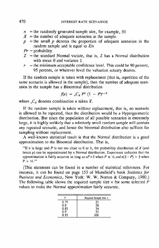
470 INTEREST RATE SCENARIOS
n = the randomly generated sample size, for example, 50 X = the number of adequate scenarios in the sample p = the small p denotes the proportion of adequate scenarios in the
random sample and is equal to X/n Pr = probability Z = the standard Normal variate, that is, Z has a Normal distribution
with mean 0 and variance 1 r = the minimum acceptable confidence level. This could be 90 percent,
95 percent, or whatever level the valuation actuary desires.
If the random sample is taken with replacement (that is, repetition of the same scenario is allowed in the sample), then the number of adequate scen- arios in the sample has a Binominal distribution
f(x) = ,Cx px (1 - p),,-x
where ,,Cx denotes combination n taken X.
If the random sample is taken without replacement, that is, no scenario is allowed to be repeated, then the distribution would be a Hypergeometric distribution. But since the population of all possible scenarios is extremely large, it is highly unlikely that a relatively small random sample will contain any repeated scenario, and hence the binomial distribution also suffices for sampling without replacement.
A well-known statistical result is that the Normal distribution is a good approximation to the Binomial distribution. That is,
" I f n is large and P is not too close to 0 or 1, the probability distribution of X (and hence p) can be approximated by a Normal distribution. Experience indicates that the approximation is fairly accurate as long as nP>5 when P < Vz and n(l -P) > 5 when P > 1/2."
(This statement can be found in a number of statistical references. For instance, it can be found on page 153 of Mansfield's book Statistics for Business and Economics, New York: W. W. Norton & Company, 1980.) The following table shows the required sample size n for some selected P values to make the Normal approximation fairly accurate.
P Required Sample Size n
0.75 21 0.8 26 0.85 34 0.9 51 0.95 101

DISCUSSION 4 7 1
Since the expected value and variance o f p are
E(p) = P
and
we know that
P(1 - P) Var (p) -
n
p - P
472 INTEREST RATE SCENARIOS
in the population. Note that:
1. For a given acceptable confidence level r, the lower bound of P (that is, the quantity to the right of the inequality) gets larger as p or n increases. Hence by increasing the sample size, the actuary can obtain a higher lower bound for P. And by trans- forming the above equation, we can easily derive the minimum sample size n needed to ensure (with some confidence level) that the difference between the sample p and the population P be less than some quantity (say 2 percent).
2. Some statisticians have recommended the use of a continuity correction in the above equation. This is a correction that is used when a discrete probability distribution (for example, binomial) is approximated by a continuous one (for example, Normal). The correction is relatively minor and is normally done by subtracting 0.5 from X (or 1/2n from p).
To assess whether the current reserve is adequate given the results of the randomly generated sample , the valuation actuary can use a procedure as follows:
1. Determine a minimum acceptable confidence level, for example, 90 percent. 2. The reserve will be considered adequate if the lower bound of P, the proportion of
adequate scenarios in the population, is at least some amount P* (for example, 0.80).
Let us illustrate the application of the procedure with a simple example. Assume that in a set of 60 randomly generated scenarios, there are 54 ad- equate scenarios. Then we can say with a 90 percent confidence that
/ 0 . 9 ( 1 - 0.9) V > 0.9 - 1.29 ~ / 60 - 0.85
where 1.29 is the Z value with 90 percent probabil i ty to the left of it. That is, there is a 90 percent probabil i ty that the proportion of adequate scenarios in the set of all possible scenarios of the model wilt be at least 0.85. If a lower bound of 0.8 is specified for P , then the reserve would be judged to be adequate.
If the actuary wants to increase the confidence level from 90 percent to 95 percent, the lower bound of P will be somewhat smaller,
/ 0 . 9 ( 1 - 0.9) P _> 0.9 - 1.645 ~ 60 - 0.84
And, for a 99 percent confidence level, the lower bound of P is 0.81.

OISCUSSION 473
Summary Unless future research clearly identifies the underlying probability distri-
bution of the ending surplus, it will be difficult for the valuation actuary to extend the randomly generated results to the population. However, the ac- tuary can use our suggested procedure to make probability statements re- garding the proportion of adequate scenarios in the set of all possible scenarios that can be generated from the creator's (actuary's) model. Such a procedure is based on well-known statistical results and is simple to apply. It is hoped that future research can uncover more elaborate and precise methods than the simple method illustrated here.
It should be reiterated that any conclusion about reserve adequacy based on the result of a model is highly dependent on the appropriateness of the model and its assumptions. The latter, plus the determination of what is adequate (80 percent, 95 percent, and so on), involves subjective judgment. To this extent, it is better to use the suggested procedure as a management analytical tool and not as a regulatory requirement.
(AUTHOR'S REVIEW OF DISCUSSION)
MERLIN F. JETTON"
I thank the discussants for their fine comments, which enhance the value of this paper.
Mr. Strommen offers some interesting variations on the third stochastic model. Regarding using a range of values for T~(®), I would advise also increasing the coefficients off(t) to achieve a more suitable behavior. With- out such a change, the mean-reversion property would be greatly weakened.
His method of calculating the twenty-year Treasury rate is creative, and it has some nice properties. It provides a built-in solution to the case for which the starting yield curve has an atypical slope. The fact that it uses parameters that can be based on historical interest rates is, I believe, a definite plus.
Mr. Gurski provides some strong statistical support for the hypothesis that changes in interest rates are normally distributed. It is a welcome addition to my paper, because the assumption is an important one and I did not furnish such support.
He describes an alternative model that has much in common with my third stochastic model. The major difference between his model and mine is the method of calculating another point on the yield curve, given only one point. His method relies more heavily on statistics, which a user may find desirable.

474 INTEREST RATE SCENARIOS
A point worth noting, however, is that heavier reliance on conventional statistical methods called for an additional constraint, because such methods fall short of mirroring the real world. Regarding my model, he states that one should use the standard deviation of the error or residual random variable e from the regression equation Y= a X + b + e rather than the standard devia- tion of the spreads. Strictly speaking, he is correct. Practically speaking, they are nearly the same.
Mr. Gurski claims that historical spreads (T2o-Tt) are not normally dis- tributed and that they are serially correlated. The question "Are historical spreads normally distributed?" has no clear answer. It depends on the data you look at and the statistical test (type and confidence level) used. In my opinion there is more than adequate justification for assuming that spreads are normally distributed. The second claim is correct, given that the time interval between measurements is short enough. I would agree that this characteristic of spreads should be recognized in a model in which interest rates are determined more frequently than semiannually or annually.
Mr. Gurski states that he has used a linear mean-reverting formula. I tested a linear formula in the course of developing my cubic formula and found it inadequate to handle the full range of differences between Tl(t) and TI(~). If the coefficient was suitable for large (small) differences, then it was too large (small) for small (large) differences.
I commend Mr. Gurski for having tested output from his model against historical interest rates.
Messrs. Buff and Lassow should be thanked for their list of references, many of which were published after my paper was submitted for publication. They raise several good questions about creating interest rate scenarios. I will respond to a couple of their questions about comparing different models.
First, they asked how scenarios based on the third stochastic model com- pare to those based on the second. It would be easiest to answer with a graph. Suppose a number of scenarios were generated from both models and frequency curves were drawn from the one-year Treasury rates generated by each model. Then the curves would be similar to those in Figure 4.
Second, they asked how important is the choice of the long-term interest rate trend assumption. Again a graph seems to be the best means of response. Suppose two sets of scenarios are generated, one with T~(00)= T,(0) and the second with T~(®) = T~(0) + 1%, and frequency curves are drawn from the one- year Treasury rates. Then the curves would be similar to those in Figure 5.

DISCUSSION 475
FIGURE 4
0.20 Second Stochastic Model (unbounded) Second Stochastic Model (bounded) Third Stochastic Model
o.15 i ' ~
0.05 . . -p " / " ~.-~'~.. .ii
2 4 6 8 10 12 14 16 Interest Rate
FIGURE 5
0.20
0.15
e.,
o O.lO
0.05
Third Stochastic Model
7", (z ) = 7", (0)
T, (~) = T, (O) + 1%
//
2 4 6 8 10 12 14 16 18 Interest Rate
Mr. Lord also deserves thanks for his references to other literature on modeling interest rates.
He points out the relative simplicity of the models presented in the paper. My goal was to provide skeletons and discuss major characteristics, which could be readily understood. I have found that much of the other literature

476 INTEREST RATE SCENARIOS
is very technical, is not made for easy reading, and/or contains models described in words without the mathematics.
Mr. Lord seems to believe that the mean reversion formula should produce a more rapid convergence toward T](c0). The formula I gave does not have much effect when the difference between Tl(t) and Tl(00) is small. I do not believe there is an objective answer here. It would be very difficult to base an answer on historical interest rates, for it would be hard to distinguish between interest rate movements that are " r andom" and those that are due to "mean reversion." Anyone who agrees with Mr. Lord can, of course, use a different formula more suitable to his/her tastes.