Interest Rate Volatility andNo-Arbitrage Affine Term Structure Models∗

Scott Joslin† Anh Le‡

This draft: April 3, 2016

Abstract

An important aspect of any dynamic model of volatility is the requirement thatvolatility be positive. We show that for no-arbitrage affine term structure models, thisadmissibility constraint gives rise to a tension in simultaneous fitting of the physicaland risk-neutral yields forecasts. In resolving this tension, the risk-neutral dynamicsis typically given more priority, thanks to its superior identification. Consequently,the time-series dynamics are derived partly from the cross-sectional information; thus,time-series yields forecasts are strongly influenced by the no-arbitrage constraints. Wefind that this feature in turn underlies the well-known failure of these models withstochastic volatility to explain the deviations from the Expectations Hypothesis observedin the data.

∗We thank Caio Almeida, Francisco Barillas, Riccardo Colacito, Hitesh Doshi, Greg Duffee, MichaelGallmeyer, Bob Kimmel, Jacob Sagi, Ken Singleton, Anders Trolle and seminar participants at theBanco de Espana - Bank of Canada Workshop on Advances in Fixed Income Modeling, Emory Goizueta,EPFL/Lausanne, Federal Reserve Bank of San Francisco, Federal Reserve Board, Gerzensee Asset PricingMeetings (evening sessions), the 2012 Annual SoFiE meeting, the 2013 China International Conference inFinance, and University of Houston Bauer for helpful comments.†University of Southern California, Marshall School of Business, sjoslin@usc.edu‡Pennsylvania State University, Smeal College of Business, anh le@psu.edu

1

1 Introduction

One of the key challenges for stochastic volatility models of the term structures, as observed byDai and Singleton (2002), is the “tension in matching simultaneously the historical propertiesof the conditional means and variances of yields.” Similarly, Duffee (2002) notes that theoverall goodness of fit “is increased by giving up flexibility in forecasting to acquire flexibilityin fitting conditional variances.” Although the difficulty in matching both first and secondmoments in affine term structure models has been a robust finding in the literature, theexact mechanism that underlies this tension is not well understood. In this paper, we showthat the key element in understanding the tension between first and second moments is theno-arbitrage restriction inducing the additional requirement to match first moments underthe risk-neutral distribution. Moreover, we show that precise inference about the risk-neutraldistribution has a number of important implications for stochastic volatility term structuremodels.

The literature has largely attributed the failures of stochastic volatility term structuremodels to match key properties in the data as the tension between the physical first andsecond moments. To see the importance of the no-arbitrage constraints, consider, for example,the deviations from the expectations hypothesis (EH). Campbell and Shiller (1991) show thatwhen the EH holds, a regression coefficient of φn = 1 should be obtained in the regression

yn−1,t+1 − yn,t = αn + φn

(yn,t − y1,t

n− 1

)+ εn,t+1, (1)

where yn,t is the n-month yield at time t. However, in the data, the empirical φn coefficientestimates are all negative and increasingly so with maturity. Dai and Singleton (2002)(hereafter DS) show that no-arbitrage models with constant volatility are consistent withthe downward sloping pattern in the data. However, the no-arbitrage models with one ortwo stochastic volatility factors are unable to match the pattern in the data. Their resultsare replicated in Figure 1.1 DS conjecture “the likelihood function seems to give substantialweight to fitting volatility at the expense of matching [deviations from the EH]”.

We estimate stochastic volatility factor models that do not impose no arbitrage but fitstochastic volatility of yields. In stark contrast to the no arbitrage models, the stochasticvolatility factor models can almost perfectly match the empirical patterns of bond riskpremia as characterized by regression coefficients. This finding clarifies that fitting stochasticvolatility is not an issue per se. Rather, it is the restrictiveness associated with the no-arbitrage structure that underlies the well documented failure of the no arbitrage stochasticvolatility models to rationalize the deviations from the EH in the data.

The tension between first and second moments arises because of the fact that volatilitymust be a positive process. This requires that forecasts of volatility must also be positive.This introduces a tension between first and second moments. This type of tension, observedby Dai and Singleton (2002) and Duffee (2002), is generally present in affine stochasticvolatility models, even when no arbitrage restrictions are not imposed. In a no arbitrage

1See Section 5 for additional details on the data and our estimation.

2

1 2 3 4 5 6 7 8 9 103

2.5

2

1.5

1

0.5

0

0.5

1

Maturity

DataA1(3)

A0(3)

A2(3)

F1(3)

F2(3)

Figure 1: Violations of the Expectations Hypothesis. This figures plots the coefficients φnfrom the Campbell-Shiller regression in (1). When risk premia are constant so that theexpectations hypothesis holds, the coefficients should be uniformly equal to one across allmaturities. The models Am(3) are three factor no arbitrage models with m = 0, 1, or 2factors driving volatility. The models Fm(3) are three factor models that do not impose noarbitrage with m = 1 or 2 factors driving volatility.

model, volatility must also be a positive process under the risk-neutral measure. This inducesan additional tension with risk-neutral first moments. This creates a three-way tension nowbetween first moments under the physical and risk-neutral measure and second moments.The relative importance of these moments (and their role in the tension) are determined bythe precision with which they can be estimated.

At the heart of our result is the fact that the Q dynamics is estimated much moreprecisely than its historical counterpart. Intuitively, although we have only one historical timeseries with which to estimate physical forecasts, each observation of the yield curve directlyrepresents a term structure of risk neutral expectations of yields. Due to this asymmetry,it is typically “costly” for standard objective functions to “give up” cross-sectional fits fortime-series fits in estimation. As a result, when faced with the “first moments” tension– the trade-off between fitting time series and risk-neutral forecasts – standard objectivefunctions typically settle on a rather uneven resolution in which cross-sectional pricing errorsare highly optimized at the expense of fits to time series forecasts. The resulting impact onthe time series dynamics in turn deprives the estimated model of its ability to replicate theCS regressions – meant to capture the times series properties of the data.

Our findings add to the recent discussion that suggests that no arbitrage restrictions arecompletely or nearly irrelevant for the estimation of Gaussian dynamic term structure models

3

(DTSM).2 Still left open by the existing literature is the question of whether the no arbitragerestrictions are useful in the estimation of DTSMs with stochastic volatility. Our results showthat the answer to this question is a resounding yes – an answer that is surprising (given theexisting evidence regarding Gaussian DTSMs) but can now be intuitively explained in lightof our results. That is, the “first moments” tension essentially provides a channel throughwhich relatively more precise Q information will spill over and influence the estimation of theP dynamics. This channel does not exist in the context of Gaussian DTSMs in which theadmissibility constraint ensuring positive volatility is not needed.

Our findings also help clarify the nature of the relationship between the no arbitrage struc-ture and volatility instruments extracted from the cross-section of bond yields documentedby several recent studies.3 For example, we show that for the A1(N) class of models (an Nfactor model with a single factor driving volatility), the cross-section of bonds will revealup to N linear combinations of yields, given by the N left eigenvectors of the risk neutralfeedback matrix (KQ

1 ), that can serve as instruments for volatility. The no arbitrage structurethen essentially implies nothing more for the properties of volatility beyond the assumed onefactor structure and the admissibility conditions. Furthermore, we show that the estimatesof KQ

1 are very strongly identified and essentially invariant to volatility considerations. For avariety of sampling and modeling choices, we show that the estimates of KQ

1 are virtuallyidentical across models with or without stochastic volatility.4 This invariance implies thestriking conclusion that a Gaussian term structure model – with constant volatility – canreveal which instruments would be admissible for a stochastic volatility model.5 An elaborateexample illustrating this point is provided in Section 5.2.

Finally, our results help identify aspects of model specifications that may or may not haveany significant bearing on the model implied volatility outputs. For example, we show thatwithin the A1(N) class of models, different specifications of the market prices of risks areunlikely to significantly affect the identification of the volatility factor. To see this, recallfrom the preceding paragraph that volatility instruments for an A1(N) model are determinedby left eigenvectors of the risk neutral feedback matrix. Intuitively, since the market prices ofrisks serve as the linkage between the P and Q measures, and since the Q dynamics is verystrongly identified, different forms of the market prices of risks are most likely to result indifferent estimates for the P dynamics while leaving estimates of risk neutral feedback matrixessentially intact. This thus implies that volatility instruments are likely identical acrossthese models with different risk price specifications. Our intuition is consistent with the

2See, for example, Duffee (2011), Joslin, Singleton, and Zhu (2011), and Joslin, Le, and Singleton (2012).3For example, Collin-Dufresne, Goldstein, and Jones (2009) find an extracted volatility factor from the

cross-section of yields through a no arbitrage model to be negatively correlated with model-free estimates.Jacobs and Karoui (2009) in contrast generally find volatility extracted from affine models are generallypositively related though in some cases they also find a negative correlation. Almeida, Graveline, and Joslin(2011) also find a positive relationship.

4In addition to our results, findings by Campbell (1986) and Joslin (2013b) also suggest that risk neutralforecasts of yields are largely invariant to any volatility considerations.

5A practical convenience of this result is that we can use the Gaussian model to generate very goodstarting points for the Am(N) models. In our estimation, these starting values take only a few minutes toconverge to their global estimates.

4

almost identical performances of volatility estimates implied by A1(3) models with different(completely affine and essentially affine) risk price specifications as reported in Jacobs andKaroui (2009).

The rest of the paper is organized as follows. In Section 2, we provide the basic intuitionas to how the “first moments” tension arises. In Section 3, we lay out the general setup ofthe term structure models with stochastic volatility that we subsequently consider. Section 4empirically evaluates the admissibility restrictions under both the physical and risk neutralmeasures. Section 5 provides a comparison between the stochastic volatility and pure gaussianterm structure models. Section 6 examines the impact of no arbitrage restrictions on various’model performance statistics. Section 8 provides some extensions. Section 9 concludes.

2 Basic Intuition

In this section, we develop some basic intuition for our results before elaborating in moredetail both theoretically and empirically. We first describe three basic moments that a termstructure model should match. We then show how tensions arise in a no arbitrage termstructure model in matching those moments. In particular, we show that the presence ofstochastic volatility induces a tension between matching first moments under the historicaldistribution (P) and the risk-neutral distribution (Q). This tension accentuates the difficultyin matching first and second moments under the historical distribution.

2.1 Moments in a term structure model

A term structure model should match:

1. M1(P): the conditional first moments of yields under the historical distribution,

2. M1(Q): the conditional first moments of yields under the risk-neutral distribution, and

3. M2: the conditional second moments of yields.6

A number of basic stylized facts are well-known about these moments (see, Piazzesi (2010)or Dai and Singleton (2003), for example.) Empirically, the slope and curvature of theyield curve (as well as the level to a slight extent) exhibit some amount of mean reversion.Also, an upward sloping yield curve often predicts (slightly) lower interest rates in thefuture. M1(P) should capture these types of patterns. Recall that risk-neutral forecasts areconvexity-adjusted forward rates and therefore matching first moments under the risk-neutralmeasure, M1(Q), is closely related to the ability of the model to price bonds. The volatility

6We make no distinction between second moments under the historical and risk-neutral distribution thoughthis is possible in some contexts. In Section 8.2 we discuss also the case where there is unspanned stochasticvolatility.

5

of yields is time-varying and persistent. Volatility is also related at least partially to the leveland shape of yield curve.7 M2 should deliver such features of volatility.

It is worth comparing that we could equivalently replace M1(Q) with matching risk premia.Dai and Singleton (2003) and others take this approach. In this context, the model shouldmatch time-variation in expected excess returns found in the data such as the fact thatwhen yield curve is upward sloping, excess returns for holding long maturity bonds are onaverage higher. Since excess returns are related to differences between actual and risk-neutralforecasts (i.e. the expected excess return is the difference between an expected future spotrate and a forward rate), such an approach is equivalent to our approach. As we explainlater, focusing on risk-neutral expectations has the benefit of isolating parameters which areboth estimated precisely and, importantly, invariant to the volatility specification.

2.2 The first moments tension

We now develop some intuition for how the “first moments” tension—that is a tension betweenmatching M1(P) and M1(Q)—arises.

Consider the affine class of models, AM (N), formalized by Dai and Singleton (2000). Dueto the affine structure, the processes for the first N principle components of the yield curve(e.g., level, slope, and curvature), denoted P , can be written as:

dPt =(K0 +K1Pt)dt+√

ΣtdBt, (2)

dPt =(KQ0 +KQ

1 Pt)dt+√

ΣtdBQt , (3)

where Bt, BQt are standard Brownian motions under the historical measure, P, and the risk

neutral measure, Q, respectively. Σt is the diffusion process of Pt, taking values as an N ×Npositive semi-definite matrix:8

Σt = Σ0 + Σ1V1,t + . . .+ ΣMVM,t, and Vi,t = αi + βi · Pt, (4)

where Vi,t’s are strictly positive volatility factors and conditions are imposed to maintainpositive semi-definite (psd) Σt.

9

7A rich body of literature has shown that the volatility of the yield curve is, at least partially, related tothe shape of the yield curve. For example, volatility of interest rates is usually high when interest rates arehigh and when the yield curve exhibits higher curvature (see Cox, Ingersoll, and Ross (1985), Litterman,Scheinkman, and Weiss (1991), and Longstaff and Schwartz (1992), among others).

8Importantly, diffusion invariance implies that the diffusion, Σt, is the same under both measures. Since Σt

is the same under both the historical and risk-neutral measures, it must be that the coefficients in (4) are thesame under both measures. A caveat applies that at a finite horizon, there may be difference in the coefficientsin (4). These arise because of differences in Et[Vt+∆t] and EQ

t [Vt+∆t]. Importantly, however, (α∆ti , β∆t

i ) willnot depend on P or Q. This differences will manifest in differences in the other coefficients. That is, therewill be (Σ∆t,Q

0 ,Σ∆t,Q1 , . . . ,Σ∆t,Q

M ) which will be different from (Σ∆t,P0 ,Σ∆t,P

1 , . . . ,Σ∆t,PM ). These differences will

not be important for our analysis. Even so, in typical applications, the time horizon is small (from daily to atmost one quarter), so even these differences will be minor. See also Section 4 and Appendix B.

9Alternatively, one could express the diffusion as Σt = Σ0 + Σ1P1,t + . . . + ΣNPN,t. When the model

falls in the AM (N) class, the matrices (Σ1, . . . , ΣN ) will lie in an M -dimensional subspaces, allowing therepresentation in (4)

6

The one-factor structure of volatility

For the sake of clarity, let us first specialize to the case: M = 1. Due to the positivity of theone volatility factor, Vt = α + β · Pt (where for simplicity we drop the indices in equation(4)), forecasts of Vt at all horizons must remain positive. Thus, to avoid negative forecasts,the (N − 1) non-volatility factors must not be allowed to forecast Vt. This in turn requiresthat the drift of Vt must depend on only Vt.

According to equation (2), the drift of Vt (ignoring constant) is given by β′K1Pt. For thisto depend only on Vt, and thus β′Pt, it must be the case that β′K1 is a multiple of β′. Thatis, β must be a left-eigenvector of K1. Equivalently, β must be an eigenvector of K ′1.

Likewise, applying similar logic under the risk-neutral measure, it must follow that β is aleft-eigenvector of KQ

1 . Thus, the volatility loading vector β must be a left eigenvector to boththe risk neutral feedback matrix, KQ

1 , and physical feedback matrix, KP1 . This establishes a

tight connection between the physical and risk neutral yields forecasts since KP1 and KQ

1 areforced to share one common left eigenvector.

With this in mind, an unconstrained estimate of KP1 , for example one obtained by fitting P

to a VAR(1) analogous to (2), may not be optimal. The reason being, such an unconstrainedestimate might force KQ

1 to admit a left eigenvector of K1 as one of its own. Such animposition can result in poor cross-sectional fits. Likewise, an unconstrained estimate of KQ

1

can significantly impact the time series dynamics, by imposing one of its own left eigenvectorsupon KP

1 . By stapling the P and Q forecasts together, the common left eigenvector constraintpotentially triggers some tradeoff as the P and Q dynamics “compete” to match M1(P) andM1(Q).

More general settings

More generally, since the volatility factors Vi,t must remain positive, their conditional expec-tations at all horizons must be positive. For given βi’s, only some values of (K0, K1) willinduce positive forecasts of Vi,t for all possible values of Pt.10 This is the well-documentedtension between matching first and second moments (M1(P) and M2) seen in the literature.We would like to choose a particular volatility instrument (βi’s) to satisfy M2, but the bestchoice of βi’s to match M2 may rule out the best choice of (K0, K1) to match M1(P).

Even within an affine factor model with stochastic volatility (that is, a factor model thatdoes not impose conditions for no arbitrage so that (2) applies but not (3)), this tension wouldarise. That is, no arbitrage does not directly affect this tension. However, for no-arbitrageaffine term structure models, the above logic applies equally to both the P and Q measures.As before, for a given choice of βi’s, we will be restricted on the choice of (KQ

0 , KQ1 ), so that

the drift of Vi,t under the risk-neutral measure guarantees that risk-neutral forecasts of Vi,tremain positive. Thus the no arbitrage structure adds a tension between M2 and M1(Q).That is, the best choice of βi’s to match M2 may be incompatible with the best choice of(KQ

0 , KQ1 ) to match M1(Q).

10In the affine model we consider, the possible values of Pt will be an affine transformation of RM+ ×RN−M

for some (M,N).

7

This implies a three-way tension between M1(P), M1(Q), and M2. When a model matchesM2 and either M1(P) or M1(Q), it may not be possible to match the other first moment.Since the risk-neutral dynamics are typically estimated very precisely, this can lead to adifficulty matching M1(P) when M2 is also matched.

3 Stochastic Volatility Term Structure Models

This section gives an overview of the stochastic volatility models that we consider. First, weestablish a general factor time-series model with stochastic volatility that does not imposeconditions for the absence of arbitrage. Within these models, arbitrary linear combinations ofyields serve as instruments for volatility. An important consideration here is the admissibilityconditions required to maintain a positive volatility process. Next, we show how no arbitrageconditions imply constraints on the general factor model. A key result that we show is thatno arbitrage imposes that the volatility instrument is entirely determined by risk neutralexpectations. Finally, we investigate further the links between volatility and the cross-sectionalproperties of the yield curve within the no arbitrage model. For simplicity, we focus in themain text on the case of a single volatility factor under a continuous time setup; modificationsfor discrete time processes and more technical details are described in Appendix B.

3.1 General admissibility conditions in latent factor models

We first review the conditions required for a well-defined positive volatility process withina multi-factor setting. Following Dai and Singleton (2000), hereafter DS, we refer to theseconditions as admissibility conditions. Recall the N -factor A1(N) process of DS. This processhas an N -dimensional state variable composed of a single volatility factor, Vt, and (N − 1)conditionally Gaussian state variables, Xt. The state variable Zt = (Vt, X

′t)′ follows the Ito

diffusion

d

[VtXt

]= µZ,tdt+ ΣZ,tdB

Pt , (5)

where

µZ,t =

[K0V

K0X

]+

[K1V K1V X

K1XV K1X

] [VtXt

], and ΣZ,tΣ

′Z,t = Σ0Z + Σ1ZVt, (6)

and BPt is a standard N -dimensional Brownian motion under the historical measure, P. Duffie,

Filipovic, and Schachermayer (2003) show that this is the most general affine process onR+ × RN−1.

In order to ensure that the volatility factor, Vt, remains positive, we need that when Vtis zero: (a) the expected change of Vt is non-negative, and (b) the volatility of Vt becomeszero. Otherwise there would be a positive probability that Vt will become negative. Imposingadditionally the Feller condition for boundary non-attainment, our admissibility conditionsare then

K1V X = 0, Σ0Z,11 = 0, and K0V ≥1

2Σ1Z,11. (7)

8

A consequence of these conditions is that volatility must follow an autonomous processunder P since the conditional mean and variance of Vt depends only on Vt and not on Xt.We now show how to embed the A1(N) specification into generic term structure modelswhere no arbitrage is not imposed and re-interpret these admissibility constraints in terms ofconditions on the volatility instruments.

3.2 An A1(N) factor model without no arbitrage restrictions

We can extend the latent factor model of (5–6) to a factor model for yields by appending thefactor equation

yt = AZ +BZZt, (8)

where (AZ , BZ) are free matrices. Importantly, there are no cross-sectional restrictions thattie the loadings (AZ , BZ) together across the maturity spectrum. In this sense, this is a purefactor model without no arbitrage restrictions.

Given the parameters of the model, we can replace the unobservable state variable withobserved yields through (8). Following Joslin, Singleton, and Zhu (2011), hereafter JSZ, wecan identify the model by observing that equation (8) implies Pt ≡ Wyt = (WAZ)+(WBZ)Ztfor any given loading matrix W such that Pt is of the same size as Zt. Assuming WBZ isfull rank,11 this in turn allows us to replace the latent state variable Zt with Pt:

dPt = (K0 +K1Pt)dt+√

Σ0 + Σ1VtdBPt , (9)

where we can write Vt (the first entry in Zt) as a linear function of Pt: Vt = α + β · Pt.Because the rotation from Z to P is affine, individual yields must be related to the yield

factors Pt through:12

yt = A+B Pt. (10)

The admissibility conditions (7) map into:

β′K1 = cβ′, (11)

where c is an arbitrary constant, and

β′Σ0β = 0, and β′K0 ≥1

2β′Σ1β. (12)

We will denote the stochastic volatility model in (9–10) by F1(N). The model is parame-terized by ΘF ≡ (K0, K1,Σ0,Σ1, α, β, A,B) which is subject to the conditions in (12). Ourdevelopment shows that the F1(N) model is the most general factor model with an underlyingaffine A1(N) state variable.

11This is overidentifying. For details, see JSZ. In the current case, this would rule out unspanned stochasticvolatility in the factor model. We extend our logic to the case of partially unspanned volatility in Section 8.

12To maintain internal consistency, we impose that WA = 0 and WB = IN , as in JSZ. This guaranteesthat as we construct the yield factors by premultiplying W to the right hand side of the yield pricing equation(10), we exactly recover Pt.

9

We will refer to the first admissibility condition in (11) as condition A(P). This condition,needed so that Vt is an autonomous process under P, can be restated as the requirement thatβ be a left eigenvector of K1. With this requirement, choosing a β such that Vt matchesyields volatility (M2) is equivalent to imposing a certain left eigenvector on the time seriesfeedback matrix K1, which may hinder our ability to match the time series forecasts of bondyields (M1(P)). When it is not possible to choose K1 to match M1(P) and β to match M2 inthe presence of A(P), a tension will arise. We refer to the tension between first and secondmoments as the difficulty to match M1(P) and M2 in the presence of the constraint A(P).

3.3 No arbitrage term structure models with stochastic volatility

The A1(N) no arbitrage model of DS represents a special case of the F1(N) model. That is,when one imposes additional constraints to the parameter vector ΘF one will obtain a modelconsistent with no arbitrage. In this section, we first review the standard formulation of theA1(N) no arbitrage model. We then focus on the the effect of no arbitrage on the volatilityinstrument through the restriction it implies on the loadings parameter β.

The latent factor specification of the A1(N) model

We now consider affine short rate models which take a latent variable Zt with dynamicsgiven by (5–6) and append a short rate which is affine in a latent state variable. We considerthe general market prices of risk of Cheridito, Filipovic, and Kimmel (2007). Joslin (2013a)shows that any such latent state term structure model can be drift normalized under Q sothat we have the short rate equation

rt = r∞ + ρV Vt + ι ·Xt, (13)

where ι denotes a vector of ones, ρV is either +1 or -1, and the canonical risk-neutral dynamicsof Zt are given by

dZt =

([KQ

0V

0N−1×1

]+

[λQV 01×N−1

0N−1×1 diag(λQX)

]Zt

)dt+

√Σ0Z + Σ1ZVtdB

Qt , (14)

where λQX is ordered. To ensure the absence of arbitrage, we impose the Feller condition thatKQ

0V ≥ 12Σ1Z,11.

No arbitrage pricing then allows us to obtain the no arbitrage loadings that replace theunconstrained version of (8) in the F1(N) model with yt = AQ

Z + BQZZt where AQ

Z and BQZ

are dependent on the parameters underlying (13-14). From this, we again can rotate Ztto Pt ≡ Wyt to obtain a yield pricing equation in terms of Pt: yt = A + BPt. This is aconstrained version of the yield pricing equation for the F1(N) model in (10). In addition tothe time series dynamics in (9), we also obtain the dynamics of P under Q:

dPt = (KQ0 +KQ

1 Pt)dt+√

Σ0 + Σ1VtdBQt , (15)

with Vt = α + β · Pt.

10

Compared to the F1(N) model, one clear distinction of the A1(N) model is the role ofthe Q dynamics (15) in determining yields loadings (A, B) and the volatility loadings β. Weprovide an in-depth discussion of this dependence below. We first explain the impact of theno arbitrage restrictions on the volatility loadings β. Next, we provide an intuitive illustrationas to how the no arbitrage restrictions will give rise to an intimate relation between the yieldsloadings B and the volatility loadings β. This compares starkly with the F1(N) models forwhich B and β are completely independent.

Implications of the no arbitrage restrictions for the factor model

Ideally, we would like to characterize the no arbitrage model as restrictions on the parametervector ΘF in the F1(N) model. In JSZ, they were able to succinctly characterize the parameterrestrictions of the no arbitrage model as a special case of the factor VAR model. In their case,essentially the main restriction was that the factor loadings (B) belongs to an N -parameterfamily characterized by the eigenvalues of the Q feedback matrix. In our current context ofstochastic volatility models, such a simple characterization is not possible because changingthe volatility parameters Σ1Z affects not only the volatility structure but also the loadingsBQZ .13 This is because higher volatility implies higher convexity and thus higher bond prices

or lower yields. The fact that Σ1Z shows up both in volatility and in yields complicates aclean characterization of the restrictions on ΘF that no arbitrage implies.

For this reason, we focus on a simpler but equally interesting question: what is the impactof the no arbitrage restrictions on the volatility loadings β?

Recall from the previous subsection that for an F1(N) model, the two main conditionson β are : (1) matching second moments (M2); and (2) β must be a left eigenvector of thephysical feedback matrix K1 that matches the first moments under P (M1(P)). Turning to theA1(N) model, these conditions are still applicable. Additionally, applying the admissibilityconditions (7) to the risk-neutral dynamics in (15) results in a set of constraints analogous to(11):

β′KQ1 = cβ′, (16)

for an arbitrary number c. We will refer to the condition in (16) for the no arbitrage modelas the admissibility condition A(Q). This implies a third condition on β for the no arbitragemodel: β must be a left eigenvector of the risk neutral feedback matrix KQ

1 that matches thefirst moments under Q (M1(Q)).

The impact of the no arbitrage restrictions on β depends on how strongly identifying thethird condition is compared to the first two. Should KQ

1 be very precisely estimated from thedata, the estimates of β for the A1(N) models are strongly influenced by A(Q). Whence it ispossible that β estimates are different across the F1(N) and A1(N) models. To anticipateour empirical results, we compare these restrictions in subsequent sections and indeed findthat the admissibility condition A(Q) (together with matching M1(Q) and M2) is essentially

13In the Gaussian case, BQZ is only dependent on the eigenvalues of the risk-neutral feedback matrix, and

not on the volatility parameters.

11

the main restriction responsible for pinning down β in no arbitrage models whereas the directtension between first and second moments implied by A(P) has virtually no impact.

Why might KQ1 be strongly pinned down in the data? Similar to JSZ, it can be shown

that the no-arbitrage restriction on KQ1 takes the following form:

KQ1 = (WBQ

Z )diag(λQ)(WBQZ )−1 (17)

where λQ = (λQV , λQX

′)′. This follows from the rotation from Z whose dynamics is given by

(14) to P. Additionally, observe that the loadings BQZ depend only on (ρV , λ

Q,Σ1Z). SinceρV is a normalization factor, it can be ignored. Σ1Z will affect the yield loadings through theJensen effects which are typically small and will be dominated by variation in risk neutralexpectations driven by λQ. Thus BQ

Z will be well approximated by loadings obtained whenΣ1Z is set to zeros. These can be viewed as loadings from a Gaussian term structure modelwhich does not have a stochastic volatility effect. Up to this approximation, the risk-neutralfeedback matrix is essentially a non-linear function of its eigenvalues, which are typicallyestimated with considerable precision (for example, see JSZ).14 Combined, this implies thatKQ

1 will be strongly identified in the data and thus β (up to scaling) is likely strongly affectedby the no arbitrage restrictions due to A(Q).

To relate to the results of JSZ, we make the above arguments relying on the approximationthat convexity effects are negligible. It is important to note that we can make our argumentmore precise without resorting to approximations by a relatively more mechanical examinationof the above steps. In particular, we show in Appendix A that the volatility instrument βis in fact, up to a constant, completely determined by the (N − 1) eigenvalues given in λQX .Coupled with the observation that λQX is typically estimated with considerable precision, it isclear that the volatility instruments are heavily affected by the no arbitrage restrictions.

The relation between yield loadings and the volatility instrument

An alternative way of understanding the impact of the no arbitrage restrictions on thevolatility instrument is through examining the linkage between yield loadings (B) and β.To begin, B and β are clearly independent for the F1(N) models since they are both freeparameters. Intuitively, for these models the yields loadings B are obtained from purelycross-sectional information: regressions of yields on the pricing factors P whereas the volatilityloadings β is obtained purely from the time series information. In contrast, in the contextof an A1(N) model, both B and β are influenced by KQ

1 . This common dependence on therisk-neutral feedback matrix forces a potentially tight linkage between these two components.For the sake of intuition, we consider below a simple example and show that for no arbitragemodels there is indeed an intimate relationship between B and β.

14Intuitively, λQ governs the persistence of yield loadings along the maturity dimension. As shown byJoslin, Le, and Singleton (2012), the estimates of the loadings (obtained, for example, by projecting individualyields onto Pt) are typically very smooth functions of yield maturities. This relative smoothness in turnshould translate into small statistical errors associated with estimates of λQ. This intuition is confirmed byexamining the results of JSZ in which λQ is estimated with considerable precision.

12

Let’s define the convexity-adjusted n-year forward rate on an one-year forward loan by:

ft(n) = EQt [

∫ t+n+1

t+n

rsds]. (18)

In the spirit of Collin-Dufresne, Goldstein, and Jones (2008) we can write the following oneyear ahead risk-neutral conditional expectation:

EQt

Vt+1

ft+1(0)ft+1(1)

= constant +

a1 0 00 0 1a2 a3 a4

Vtft(0)ft(1)

. (19)

The first row is due to the autonomous nature of Vt. The second row is the definition ofthe forward rate in (18) for n = 1. The last row is obtained from the fact that in a threefactor affine model, (Vt, ft(0), ft(1)) are informationally equivalent to the three underlyingstates at time t. From the last row and by applying the law of iterated expectation to (18),we have:

ft(2) = constant + a2Vt + a3ft(0) + a4ft(1). (20)

This equation may be solved to give Vt in terms of ft(0), ft(1), and ft(2). Furthermore, since(18) gives ft+1(2) = EQ

t+1[ft+2(1)] we can use (19) and (20) to express EQt [ft+1(2)] in terms of

ft(0), ft(1), and ft(2). Putting these together allows us to substitute Vt out from (19) andobtain

EQt

ft+1(0)ft+1(1)ft+1(2)

= constant +

0 1 00 0 1α1 α2 α3

ft(0)ft(1)ft(2)

. (21)

Simple calculations give α1 = −a1a3, α2 = a3 − a1a4, and α3 = a4 + a1. It follows from thelast row of (21) that:

ft(3) = constant + α1ft(0) + α2ft(1) + α3ft(2). (22)

Equation (22) reveals that if the forward rates can be empirically observed, the loadings αcan in principle be pinned down simply by regressing ft(3) on ft(0), ft(1), and ft(2). Basedon the mappings from (a1, a3, a4) to α, it follows that the regression implied by (22) will alsoidentify all the a coefficients, except for a2. In the context of equation (20), it means that thevolatility factor is tightly linked to the forward loadings, up to a translation and scaling effect.Since forwards and yields (and therefore yield portfolios) are simply rotated representationsof one another, this implies a close relationship between the volatility instrument and yieldsloadings.

As is well known, yields and forwards at various maturities exhibit very high correlations.The R2’s obtained for cross-sectional regressions similar to (22) are typically close to 100%with pricing errors in the range of a few basis points. Therefore we expect the standard errorsassociated with α to be small and thus the volatility loadings β will be strongly identifiedfrom cross-sectional loadings.

13

Repeated iterations of the above steps allow us to write any forward rate ft(n) as a linearfunction of (f(0)t, ft(1), ft(2)). Suppose that we use J + 1 forwards in (ft(0), . . . ft(J)) inestimation, then:

ft(0)ft(1)ft(2)ft(3)ft(4)

...ft(J)

=

1 0 00 1 00 0 1α1 α2 α3

g4(α). . .gJ(α)

ft(0)ft(1)ft(2)

where (g4, . . . , gJ) represent the cross-sectional restrictions of no-arbitrage. This allows us tothink of the no-arbitrage restrictions as having two facets. First, it imposes a cross-sectionto time series link through the fact that fixing α constrains what the volatility factor mustlook like, through a3 and a4. Second, it induces cross-sectional restrictions on the loadings(g4, . . . gJ), just as is seen with pure Gaussian term structure models.

4 Evaluating the Admissibility Restrictions

We have seen in Section 3 that in order to have a well-defined admissible volatility process,we must have both A(P) and A(Q) which can be restated as that β must be a common lefteigenvector of the feedback matrices under P and Q. These admissibility restrictions arehelpful in providing guidance on potential volatility instruments. For example, although levelis known to be related to volatility, it is unlikely to be an admissible instrument for volatilityby itself. To see this, recall the well-known result (for example Campbell and Shiller (1991))that the slope of the yield curve predicts future changes in the level of interest rates. Up tothe associated uncertainty of such statistical evidence, this suggests that the slope of the yieldcurve predicts the level and thus also that the level of interest rates is not an autonomousprocess.

We evaluate empirically how helpful each of the admissibility restrictions can be inidentifying the potential volatility instrument which in turn depends on the accuracy withwhich the feedback matrices can be estimated. For example, if the physical (risk-neutral)feedback matrix is strongly identified in the data, then the condition A(P) (A(Q)) mustprovide helpful identifying information about β. As will be seen, our assessments are relativelyrobust to the extent that we do not have to actually estimate the term structure models, nordo we require that M2 be matched. Following Joslin, Le, and Singleton (2012) (hereafter JLS),we use the monthly unsmoothed Fama Bliss zero yields with eleven maturities: 6–month,one- out to ten-year. We start our sample in January 1973, due to the sparseness of longermaturity yields prior to this period, and end in December 2007 to ensure our results are notinfluenced by the financial crisis.

We note that the affine dynamics for P in (9) implies that the one month ahead conditional

14

expectation of Pt+∆ is affine in Pt:

Et[Pt+∆] = constant + eK1∆Pt (23)

where ∆ = 1/12. Thus Pt, even when sampled monthly, follows a first order VAR. Importantly,we can show that any left eigenvector of K1 must also be a left eigenvector of the one-monthahead feedback matrix eK1∆, denoted by K1,∆.15 In other words, the set of left eigenvectorsof the instantaneous feedback matrix K1 and the one-month ahead feedback matrix K1,∆

must be identical. As a result, we can equivalently restate A(P) as the requirement that thevolatility loading β be a left eigenvector of K1,∆. Since our data are sampled at the monthlyinterval, it is more convenient for us to focus on K1,∆ in our empirical analysis.

Similarly, the affine dynamics in (15) under Q also implies a first order VAR for Ptsampled at the monthly frequency:

EQt [Pt+∆] = constant+ eK

Q1 ∆︸ ︷︷ ︸

KQ1,∆

Pt. (24)

Applying similar logic, we can again restate A(Q) as the requirement that the volatilityloading β be a left eigenvector of the one-month ahead risk-neutral feedback matrix KQ

1,∆.

It is worth noting that for small ∆, KQ1,∆ ≈ I + ∆KQ

1 . So in some sense, we can view KQ1

and KQ1,∆ interchangeably. Importantly though, as the arguments above illustrate, our results

do not rely on this approximation.

4.1 Admissibility restrictions under PWe first consider the restriction A(P) which is present in both the F1(N) and A1(N) models.This restriction guarantees that Vt is an autonomous process, which in turn is necessary forvolatility to be a positive process under P. This requires the volatility instrument, β, be aleft eigenvector of the one-month ahead physical feedback matrix K1,∆. To the extent thatthe conditional mean is strongly identified by the time-series, this condition will pin downthe admissible volatility instruments up to a sign choice and the choice of which of the N lefteigenvectors instruments volatility. However, in general even with a moderately long timeseries, such as our thirty five year sample, inferences on the conditional means are not veryprecise.

To gauge how strongly identified the volatility instrument is from the autonomy require-ment under P, we implement the following exercise. First we estimate an unconstrained VARon the first three principal factors, Pt. Ignoring the intercepts, the estimates for our sample

15To see this, assume that β is a left eigenvector of K1 with a corresponding eigenvalue c. Applying thedefinition of left eigenvector, β′K1 = cβ′, repeatedly, it follows that β′Kn

1 = cnβ′ or β is also a left eigenvectorof Kn

1 for any n. Substitute these into eK1∆ =∑∞

n=0Kn1 ∆n/n!, it implies that β′eK1∆ = ec∆β′. Thus β is a

left eigenvector of eK1∆ with the corresponding eigenvalue ec∆.

15

period are:

Pt+∆ = constant +

0.9902 −0.0092 −0.04720.0097 0.9548 −0.0802−0.0021 0.0096 0.7991

︸ ︷︷ ︸

K1,∆

Pt + noise. (25)

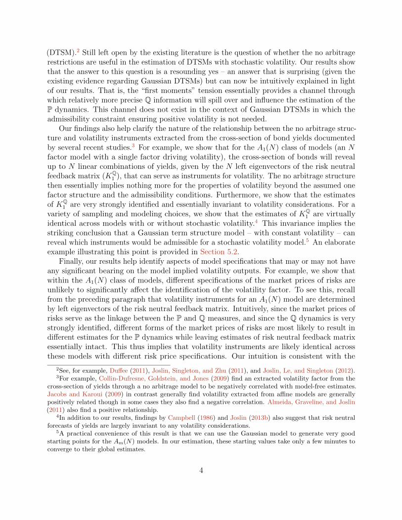
Then, for each potential volatility instrument β · Pt (as β roaming over all possible choices),we re-estimate the VAR under the constraint that β is a left eigenvector of K1,∆. The VARis easily estimated under this constraint after a change of variables so that the eigenvectorconstraint becomes a zero constraint (compare the constraints in (7) and (12)). We thenconduct a likelihood ratio test of the unconstrained versus the constrained alternative andcompute the associated probability value (p-value). A p-value close to one indicates that theevidence is consistent with such an instrument being consistent with A(P) while a p-valueclose to zero indicates contradicting evidence.16 In conducting this experiment, we do notforce β ·Pt to forecast volatility nor is β required to satisfy A(Q). In this sense, this exercise isinformative about the contribution of A(P) in shaping the volatility instrument independentof both A(Q) and the requirement that M2 be matched.

Since β · Pt and its scaled version, cβ · Pt, for any constant c, effectively give the samevolatility factor (and hence deliver the same p-values in our exercise), we scale so that allelements of β sum up to one (the loading on PC1 β(1) = 1 − β(2) − β(3)). We plot thep-values against the corresponding pairs of loadings on PC2 and PC3 in Figure 2. For easeof presentation, in this graph the three PCs are scaled to have in-sample variances of one.

We see that there are three peaks which correspond to the three left eigenvectors of themaximum likelihood estimate of K1,∆. When β is equal to one of these left eigenvectors (up toscaling), the likelihood ratio test statistic must be zero and hence the corresponding p-valuemust be one, by construction. As our intuition suggests, many, though not all, instrumentsappear to potentially satisfy A(P) according to the metric that we are considering. Thuswe conclude that the admissibility requirement under the P measure in general still leaves agreat deal of flexibility in forming the volatility instrument.

4.2 Admissibility restrictions under QTurning to A(Q), to have a clean comparison, it is ideal if we can implement the sameregression approach applied to A(P) in the previous exercise. That is, we first run anunconstrained regression using the Q forecasts:

EQt [Pt+∆] = constant+KQ

1,∆Pt + noise (26)

to obtain an estimate of KQ1,∆. An important difference here with the P case in (25) is that

we now use EQt [Pt+∆] instead of Pt+1 on the left hand side in the regression. Next, for

16We view this test as an approximation since it assumes volatility of the residuals is constant. However,computations of p-values, accounting for heteroskedasticity of the errors, deliver very similar results.

16

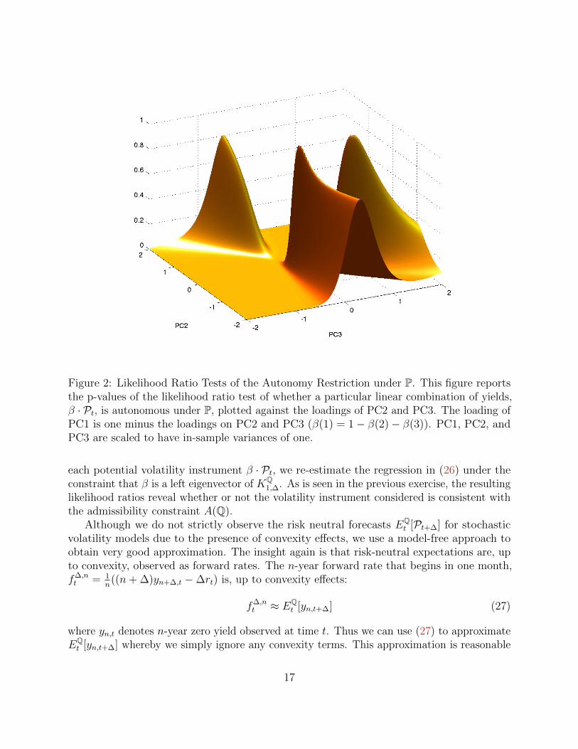
Figure 2: Likelihood Ratio Tests of the Autonomy Restriction under P. This figure reportsthe p-values of the likelihood ratio test of whether a particular linear combination of yields,β · Pt, is autonomous under P, plotted against the loadings of PC2 and PC3. The loading ofPC1 is one minus the loadings on PC2 and PC3 (β(1) = 1− β(2)− β(3)). PC1, PC2, andPC3 are scaled to have in-sample variances of one.

each potential volatility instrument β · Pt, we re-estimate the regression in (26) under theconstraint that β is a left eigenvector of KQ

1,∆. As is seen in the previous exercise, the resultinglikelihood ratios reveal whether or not the volatility instrument considered is consistent withthe admissibility constraint A(Q).

Although we do not strictly observe the risk neutral forecasts EQt [Pt+∆] for stochastic

volatility models due to the presence of convexity effects, we use a model-free approach toobtain very good approximation. The insight again is that risk-neutral expectations are, upto convexity, observed as forward rates. The n-year forward rate that begins in one month,f∆,nt = 1

n((n+ ∆)yn+∆,t −∆rt) is, up to convexity effects:

f∆,nt ≈ EQ

t [yn,t+∆] (27)

where yn,t denotes n-year zero yield observed at time t. Thus we can use (27) to approximateEQt [yn,t+∆] whereby we simply ignore any convexity terms. This approximation is reasonable

17

for two reasons. First, Jensen terms are typically small. Second, notice that since our primaryinterest is not in the level of expected-risk neutral changes but in their variation (as capturedby KQ

1,∆), it is only changes in stochastic convexity effects that will violate this approximation.Thus to the extent that changes in convexity effects are small this approximation will bevalid for inference of KQ

1,∆.

Using this method, we extract observations on EQt [yn,t+∆] from forward rates which we

can then convert into estimates of EQt [Pt+∆] using the weighting matrix W . We denote this

approximation of EQt [Pt+∆] by Pft . Whence regression (26) translates into:

Pft = constant+KQ1,∆Pt + noise. (28)

Regression (28) draws a nice analogy to the time series VAR(1) of (25) that we use inexamining A(P). Importantly, as this regression can be implemented completely independently,abstracting from any time series considerations, it serves as a stand-alone assessment of A(Q),up to the validity of our convexity approximation approach. Notably, (28) makes clear the(essentially) contemporaneous nature of the estimation of KQ

1,∆. Since Pt explains virtually all

contemporaneous yields and forwards (and thus portfolios of forwards such as Pft ), the R2’sof (28) are likely much higher than those for the time series VAR(1) at the monthly frequency.Therefore we expect much stronger identification for KQ

1,∆. Intuitively, although we observeonly a single time series under the historical measure with which to draw inferences, weobserve repeated term structures of risk-neutral expectations every month and this allows usto draw much more precise inferences.

Figure 3 plots the p-values for this test of the restrictions of various instruments to beautonomous under Q. In stark contrast to Figure 2 and in accordance with our intuition,we see that the risk-neutral measure provides very strong evidence for which instrumentsare able to be valid volatility instruments. Most potential volatility instruments are stronglyruled out with p-values essentially at zero. Thus, our results here suggest that were it onlyup to A(P) and A(Q) to decide which volatility instrument to use, the latter would almostsurely be the dominant force, with the remaining degrees of freedom being the sign choice andchoosing which of the N left eigenvectors of KQ

1,∆ is the volatility instrument. This evidencesuggests that the no arbitrage restrictions can potentially have very strong impact in shapingvolatility choices.

Left open by the model-free nature of our analysis in this section is, among other things,the possibility that the defining property of the volatility factor (β should match M2) can bepowerful enough that it might dominate A(Q) at identifying potential volatility instruments.We take up an in depth examination of this possibility in the next section.

5 Comparison of Gaussian and Stochastic Volatility

Models

To understand the contribution of matching M2 on the identification of the volatility loadingsβ, we estimate and compare the (Gaussian) A0(N) models with stochastic volatility models.

18

Figure 3: Likelihood Ratio Tests of the Autonomy Restriction under Q. This figure reportsthe p-values of the likelihood ratio test of whether a particular linear combination of yields,β · Pt, is autonomous under Q, plotted against the loadings of PC2 and PC3. The loading ofPC1 is one minus the loadings on PC2 and PC3 (β(1) = 1− β(2)− β(3)). PC1, PC2, andPC3 are scaled to have in-sample variances of one.

19

N = 4 N = 3

A0(N)

0.998 0.027 0.032 0.014 0.997 0.028 0.025-0.007 0.957 -0.128 -0.042 -0.003 0.954 -0.098-0.010 0.006 0.895 -0.080 -0.005 -0.002 0.928-0.009 -0.009 -0.085 1.007

A1(N)

0.999 0.027 0.030 0.013 0.998 0.028 0.024-0.005 0.959 -0.123 -0.037 -0.002 0.955 -0.097-0.010 0.006 0.902 -0.075 -0.005 -0.000 0.931-0.006 -0.007 -0.079 1.018

A2(N)

0.998 0.028 0.031 0.013 0.997 0.029 0.025-0.005 0.956 -0.125 -0.040 -0.002 0.954 -0.099-0.009 0.003 0.899 -0.077 -0.005 -0.002 0.929-0.005 -0.012 -0.080 1.010

Regression

0.998 0.027 0.029 0.014 0.997 0.027 0.025-0.008 0.957 -0.118 -0.041 -0.003 0.958 -0.098-0.011 0.005 0.905 -0.077 -0.006 0.007 0.925-0.016 -0.006 -0.065 0.987

Table 1: KQ1,∆ Estimates.

Clearly, matching M2 is relevant only in the latter and not the former. Since the A0(N)models are affine models, the one month ahead conditional expectation of yields portfolios Palso take an affine form. Thus for both Gaussian and stochastic volatility models, we canwrite: EQ

t [Pt+∆] = constant +KQ1,∆Pt under the risk neutral measure. Of particular interest

is the estimates of the monthly risk-neutral feedback matrix, KQ1,∆, implied by these models.

As we will show in this section, estimates of KQ1,∆ are highly similar across these models.

This suggests that the role of stochastic volatility (matching M2) is inconsequential for theestimation of KQ

1,∆. Thus identifying volatility instrument (β) is simply limited to making

the choice of which left eigenvector of KQ1,∆ and its sign can best match M2. We use the same

dataset as in the preceding section and note that all of our results remain fully robust for ashortened sample period that excludes the Fed experiment regime.

5.1 Comparison of KQ1,∆ estimates

We estimate AM(N) models, with M = 0, 1, 2 and N = 3, 4, and then rotate the statevariables into low order yield PCs. For estimation, we assume these PCs are priced perfectlywhile higher order PCs are observed with i.i.d. errors. JLS show that this assumption isinnocuous as it is likely to deliver estimates close to those obtained by Kalman filtering whereall yields portfolios are observed with errors. Estimation details and full parameter estimatesare deferred to Appendix C.

20

Table 1 reports the estimates of KQ1,∆ implied by these models. Recall the defining property

of KQ1,∆ given by equation (26) in which KQ

1,∆ is informative about how Pt forecasts Pt+∆

under the risk neutral measure. Since for each N , Pt is characterized by the same loadingmatrix W (that corresponds to the first N PCs of bond yields) across all models, it followsthat KQ

1,∆ estimates are directly comparable across all models with the same number of

factors N . Focusing first on the two models A0(3) and A1(3), the two estimates of KQ1,∆ are

strikingly close: most entries are essentially identical up to the third decimal place. Thisevidence indicates that the identification by the cross-sectional information (and possiblyother moments shared between the A0(3) and A1(3) models) for the parameter KQ

1,∆ seemsoverwhelmingly stronger than the restrictions coming from matching M2. Enriching thevolatility structure to M = 2 does not overturn this observation: the KQ

1,∆ estimate implied bythe A2(3) model remains essentially identical. Additionally, changing the number of factorsto N = 4 (results also reported Table 1) or N = 2 (results not reported) does not alter ourobservation.

We have argued that variation in the one month ahead risk-neutral expectations, asdetermined by KQ

1,∆, is well approximated by the regression based estimate of (28). Thisestimate can be further improved by simple steps that take into account the affine structureof bond yields. Specifically up to convexity effects, the affine structure of bond yields impliesthat:

Bn+∆ = KQ1,∆Bn + B∆

where Bn denotes the unannualized loadings of n-year zero yields on Pt. This suggests wecan recover KQ

1,∆ in two steps. First, we project yields of all maturities onto the states Pt to

recover the loadings Bn.17 Second, an estimate of KQ1,∆ is obtained by projecting Bn+∆ − B∆

onto Bn (allowing for no intercepts).18 As can be viewed from the last panel of Table 1, thismodel free estimate of KQ

1,∆ come strikingly close to estimates obtained from the no arbitragemodels. This evidence suggests that the cross-sectional information alone is sufficient to pindown the risk-neutral feedback matrix, and this identification is so strong that informationfrom other constraints imposed by the models seems irrelevant.

Given the estimates of AM(N) models, we are able to confirm that the convexity effectson yield loadings are negligible. Specifically, holding N fixed, varying M , and thereby varyingthe degree of convexity effects due to the presence of stochastic volatility, is completelyinconsequential for the yield loadings implied by different models. Graphs (not reported) ofyield loadings on Pt plotted against the corresponding maturities (up to ten years) impliedby A0(N), A1(N), and A2(N) are virtually indistinguishable.

The observed invariance property of KQ1,∆ estimates has a number of implications. First,

as stated previously, this allows us to pin down the potential volatility instruments using thecross-section of yields due to the admissibility constraint. Essentially the volatility instrumentis free in terms of the sign but must be one of the left eigenvectors of KQ

1,∆ which can be

17To obtain yields for the full range of maturities from the small set of maturities used in estimation, wecan use simple interpolation techniques such as the constant forward bootstrap or simply a cubic spline.

18de los Rios (2013) develops a similar regression-based approach to obtain estimates of KQ1,∆.

21

computed accurately from either the cross-sectional regression or from estimation of theA0(N) model which has constant volatility and can be estimated quite quickly as shown inJSZ.

This observation also shows that, in some regards, the estimation of the no arbitrageA1(N) model is more tractable than estimate of the F1(N) model. In the case of the Gaussianmodels the opposite holds: the factor model is trivial to estimate as it amounts to a set ofordinary least squares regressions while the no arbitrage model is slightly more difficult toestimate due to the non-linear constraints in the factor loadings. In the stochastic volatilitymodels, the admissibility conditions require a number of non-linear constraints in orderto ensure that volatility remains positive. The no arbitrage model essentially determinesthe volatility instrument up to sign and choice of eigenvector. This actually simplifies theestimation since it reduces the set of non-linear constraints that need to be imposed.

The observation that KQ1,∆ estimates are nearly invariant across Gaussian and stochastic

volatility models leads us to the surprising conclusion that the A0(N) model with constantvolatility allows us to essentially identify (up to choice of which eigenvector) the source ofstochastic volatility in the A1(N) model. We provide an illustration of this point in the nextsubsection.

5.2 Volatility information revealed by the Gaussian model

Despite the similarity, the estimates of KQ1,∆ reported in Table 1 still exhibit slight numerical

differences. It is possible these small numerical differences might become more significantin terms of the left eigenvectors and thus among model implied volatility instruments. Toshow that this is not the case, we carry out the following exercise. Starting with the KQ

1,∆

estimate by the A0(3) model, we form three potential volatility instruments from the threeleft eigenvectors of KQ

1,∆ and then pick out the instrument with most predictive contentfor volatility. Specifically, we first project the level factor, P1,t+∆, onto Pt to obtain theforecast residuals and then choose the volatility candidate with most predictive content forthe squared residuals. This way, from the A0(3) model, we can have a “guess” for what thevolatility instrument of the A1(3) model looks like even before we actually estimate the A1(3)model. Finally, we compare this “guess” to the actual volatility instrument implied by theA1(3) model.

Table 2 reports the adjusted R2 statistics (in percentage) of regressions in which eachpotential volatility instrument is used to predict the squared residuals of the level factor.Evidently, one of the instruments clearly dominates the others at all forecasting horizonsfrom one to twelve months. Comparing this dominant instrument to the actual volatilityfactor of the A1(3) model results in a striking correlation of one. To see this more visually, weplot these two volatility instruments, normalized to have the same scaling and intercepts,19

in Figure 4. Clearly, the A0(3)’s “guess” is very accurate as the two graphs are right on topof one another.

19Specifically, in constructing both volatility instruments, we drop the intercepts and scale the loading onthe level factor (β(1)) to one.

22

Horizon Instrument 1 Instrument 2 Instrument 3

1 9.35 -0.00 0.582 8.84 -0.21 -0.163 8.66 0.92 2.174 7.32 0.96 2.555 6.51 0.50 1.846 6.04 -0.24 0.127 5.28 -0.07 0.578 4.71 -0.24 0.019 4.87 0.33 1.2610 4.59 0.51 1.6611 4.27 0.51 1.7712 4.21 0.03 0.95

Table 2: R2 (in percentage) predicting squared residuals in forecasting the level factor bythe three potential volatility instruments implied by the A0(3) model. Instruments 1, 2, 3are formed from the left eigenvectors of the KQ

1,∆ matrix, corresponding to the eigenvaluesordered from highest to lowest.

1970 1975 1980 1985 1990 1995 2000 2005 20100.04

0.06

0.08

0.1

0.12

0.14

0.16

0.18

A0(3) guessA1(3)

Figure 4: Volatility instrument “guessed” by the A0(3) model and the actual volatility factorimplied by the A1(3) model. The volatility instrument is normalized as β · Pt where β(1) isscaled to one.

23

This exercise and the content of the previous subsection clearly reveal the respective rolesof the cross-sectional and time series information in shaping the choice of volatility instrumentin an A1(3) model. The cross-sectional information pins down the risk-neutral feedbackmatrix KQ

1,∆. The identification seems so strong that time series constraints from matchingM1(P) and M2 appear inconsequential. Regardless of whether the time series constraints areapplied (in the A1(3) model) or not (in the A0(3) model), the estimates of KQ

1,∆ seem largely

unaffected. The precise estimate of KQ1,∆ together with A(Q) dramatically reduces the choice

of potential volatility instruments from an uncountably infinite set to a discrete choice amongthe N left eigenvectors of KQ

1,∆. This is the very sense in which a constant volatility modelsuch as the A0(N) model can reveal volatility information of stochastic volatility models.The A0(N) model pins the optimal volatility instrument to be one of the N left eigenvectors,but it does not determine exactly which one. It is the role of the time series constraints inpicking the left eigenvector (and its sign) that best matches M1(P) and M2.

6 No Arbitrage Restrictions

In this section, we show that the clear distinction of the roles of cross-section and timeseries information in determining the volatility of no arbitrage models can have importantimplications for dynamic term structure models. Specifically, we reconsider the puzzling resultof Dai and Singleton (2002). They show that while Gaussian models are able to replicate thedeviations from the expectation hypothesis found in the data, affine term structure modelswith stochastic volatility are unable to match the patterns found in the data. This failuremay potentially be due to the tension between first and second moments. However, we showthat the stochastic volatility factor model (where the first and second moment tension stillapplies) is able to match deviations from the expectations hypothesis. This demonstratesthat the tension created by also matching M1(Q) in addition to M1(P)and M2 is what drivesthe failures of the stochastic volatility models demonstrated by Dai and Singleton (2002).

These results, together with our previous results, show that recent results about theirrelevancy of no arbitrage restrictions in Gaussian models do not extend to affine modelswith stochastic volatility. For example, Duffee (2011), Joslin, Singleton, and Zhu (2011), andJoslin, Le, and Singleton (2012) all show that no arbitrage is nearly irrelevant in Gaussiandynamic term structure models on a number of dimensions. In contract, for the case ofstochastic volatility models, the no arbitrage constraints on the factor model has materialeffects for both first and second moments.

6.1 Expectation hypothesis

A generic property of arbitrage-free dynamic term structure models is that risk-premiumadjusted expected changes in bond yields are proportional to the slope of the yield curve.Under the expectation hypothesis (EH), risk premiums are constant. This implies that the

24

coefficients φn in the projections

Proj [yn−∆,t+∆ − yn,t|yn,t − y∆,t] = αn + φn

(yn,t − y∆,t

n−∆

), for all n > ∆, (29)

should be uniformly ones under the EH. Campbell and Shiller (1991) shows robust evidencethat φn’s are significantly different from one and become increasingly negative for large n’s.This puzzling pattern of φn’s, which can be observed in Figure 1 for our sample period, hasbecome one of the most studied empirical phenomena for the last twenty years.

Dai and Singleton (2002) show that constant volatility models are not “puzzled” by thispattern and that the population coefficients φn implied by estimated A0(N) models veryclosely match their data counterparts. However, Dai and Singleton (2002) show a starkcontrast for the canonical models AM (N) models with M > 0 with stochastic volatility. Herethey find φn’s typically stay close to the unit line, thereby counter-factually implying thatthe EH nearly holds.

What is behind the difference in performances of the Gaussian and stochastic volatilitymodels? To begin, it is worth noting that the loadings φn’s for all affine models (with orwithout no arbitrage restrictions) can be written as:

φn = (n−∆)(Bn−∆K1,∆ −Bn)Σ(Bn −B∆)′)

(Bn −B∆)Σ(Bn −B∆)′. (30)

where Σ denotes the unconditional covariance matrix of the time series innovations andBn the loadings of the n-period yield yn,t on the principal components of yields Pt. Asnoted earlier, the loadings B’s are essentially identical across models with and withoutstochastic volatility.20 Furthermore, the covariance matrix Σ appears in both the numeratorand denominator of (30), thus its impact on φn is greatly dampened due to cancellation. Thisessentially leaves the one-month ahead physical feedback matrix K1,∆ as the natural focus inexplaining the differences in φn’s across the constant and stochastic volatility models.

One of the main findings of JSZ in the context of the Gaussian models is that no arbitragerestrictions are irrelevant for models’ forecasting performance. Equivalently, estimates of theone-month ahead physical feedback matrix K1,∆ from A0(N) models are exactly identical tothose obtained from OLS regressions of Pt+∆ on Pt and, thus, completely unaffected by noarbitrage restrictions. Turning to the A1(N) models, the concurrent presence of A(P) andA(Q) builds a strong link between the one-month ahead physical and risk neutral feedbackmatrices: K1,∆ and KQ

1,∆ must share one common left eigenvector. To the extent that KQ1,∆ is

very strongly pinned down by the cross-section information, it is likely to force the physicalfeedback matrix K1,∆ to accept one of the N left eigenvectors of KQ

1,∆ as one of its own.

Due to this coupling of K1,∆ and KQ1,∆, the estimate of K1,∆ from the A1(N) model is likely

strongly influenced by the no arbitrage restrictions and thus can be quite different from itsOLS counter-part.

20In fact, these loadings are very close to those obtained from OLS regressions of yields of individualmaturities onto the pricing factors Pt.

25

N = 4 N = 3

A0(N)

0.990 -0.009 -0.047 -0.017 0.990 -0.009 -0.0470.010 0.955 -0.080 -0.032 0.010 0.955 -0.080-0.002 0.010 0.799 0.030 -0.002 0.010 0.7990.000 0.012 -0.012 0.627

A1(N)

0.990 0.015 0.002 -0.034 0.993 0.011 -0.0350.004 0.975 -0.080 -0.099 0.006 0.973 -0.1000.000 0.002 0.835 0.013 -0.001 -0.009 0.823-0.006 0.001 -0.031 0.703

A2(N)

0.987 0.017 0.035 -0.004 0.992 0.015 0.009-0.002 0.958 -0.083 -0.106 0.004 0.974 -0.0750.002 0.013 0.870 0.052 0.013 0.011 0.9020.001 0.020 -0.025 0.729

F1(N)

0.991 -0.013 -0.093 -0.010 0.997 -0.018 -0.0810.006 0.962 -0.054 -0.045 0.002 0.965 -0.0520.009 -0.012 0.867 0.048 0.005 -0.008 0.830-0.009 0.022 0.003 0.715

F2(N)

0.994 -0.013 -0.086 0.028 0.998 -0.018 -0.0560.005 0.962 -0.067 -0.070 0.005 0.965 -0.0100.005 -0.012 0.876 0.032 0.004 -0.007 0.828-0.003 -0.011 -0.027 0.702

Table 3: K1,∆ Estimates

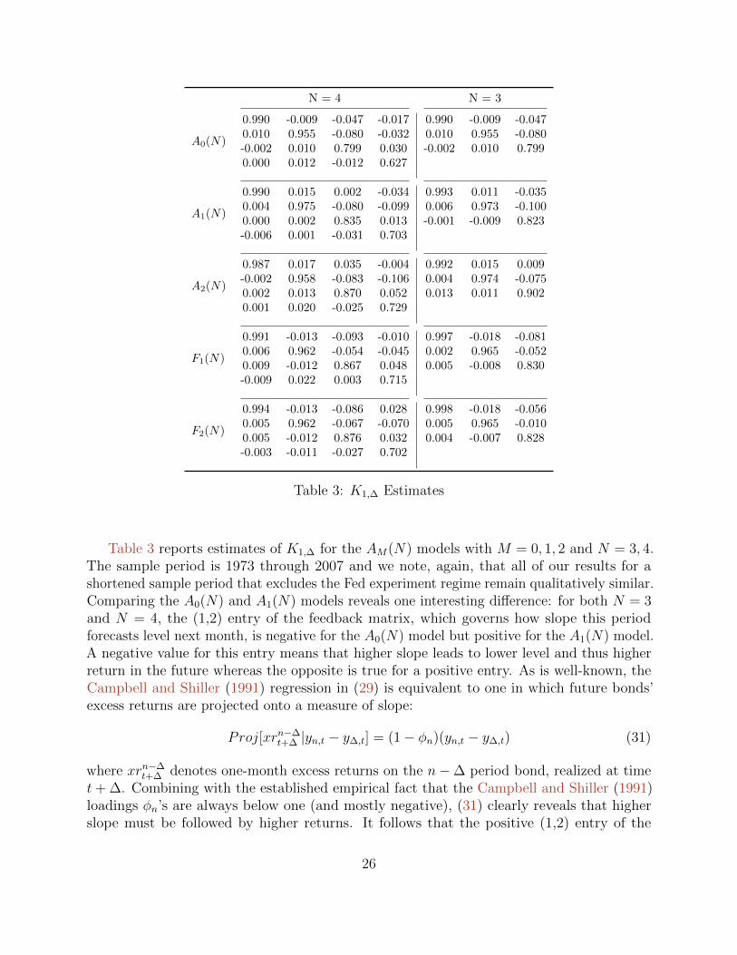
Table 3 reports estimates of K1,∆ for the AM(N) models with M = 0, 1, 2 and N = 3, 4.The sample period is 1973 through 2007 and we note, again, that all of our results for ashortened sample period that excludes the Fed experiment regime remain qualitatively similar.Comparing the A0(N) and A1(N) models reveals one interesting difference: for both N = 3and N = 4, the (1,2) entry of the feedback matrix, which governs how slope this periodforecasts level next month, is negative for the A0(N) model but positive for the A1(N) model.A negative value for this entry means that higher slope leads to lower level and thus higherreturn in the future whereas the opposite is true for a positive entry. As is well-known, theCampbell and Shiller (1991) regression in (29) is equivalent to one in which future bonds’excess returns are projected onto a measure of slope:

Proj[xrn−∆t+∆ |yn,t − y∆,t] = (1− φn)(yn,t − y∆,t) (31)

where xrn−∆t+∆ denotes one-month excess returns on the n−∆ period bond, realized at time

t+ ∆. Combining with the established empirical fact that the Campbell and Shiller (1991)loadings φn’s are always below one (and mostly negative), (31) clearly reveals that higherslope must be followed by higher returns. It follows that the positive (1,2) entry of the

26

feedback matrix, which counter-factually implies that higher slope must be followed by lowerreturns, is likely the key weak point of the A1(N) models. Moreover, the same weakness alsoapplies to the A2(N) models as the (1,2) entries for these models are also similarly positive.

To examine whether the no-arbitrage restrictions are indeed forcing the physical feedbackmatrix of the stochastic volatility models to admit these counter-factual values, we estimatethe FM(N) models established in Section 3. Recall that these are the counter-parts to theAM(N) models with the no-arbitrage restrictions, and thus the “first moments” restrictionsthrough A(P), completely relaxed. We use the same sample period (1973 through 2007)and the same set of yields in estimation, thus the estimated FM(N) and AM(N) models aredirectly comparable. Examining the reported values of the K1 matrix reported in the lasttwo panels of Table 3, for all four FM(N) models (M=1,2 and N=3,4) the (1,2) entry of thefeedback matrix is negative.

Although a negative (1,2) entry should now allow slope to forecast level with the rightsign, the key question is whether the FM(N) models, without no arbitrage restrictions, canproduce loadings φn’s that match up with the Campbell and Shiller (1991) regression (31)in the data. The answer to this question is a definite yes! Examining the pattern of theloadings φn implied by the A1(3) and A2(3) models in Figure 1, we find the well-known resultof Dai and Singleton (2002) in which these stochastic volatility models have a long way to goin matching the empirical Campbell and Shiller (1991) regression coefficients. Nevertheless,once the no arbitrage restrictions are dropped and the the A1(3) and A2(3) models turn intothe corresponding F1(3) and F2(3) models, the model-implied φn’s now become extremelyclose to their empirical counter-parts, arguably as close as those loadings implied by theA0(3) model. A graph (not reported) for four factor models shows very similar results.

In short, Figure 1 constitutes convincing evidence that the no arbitrage restrictions, andin particular needed to match M1(Q), seem directly behind the failure of the AM (N) modelsfor M > 0 in explaining the deviations from the EH. In stark contrast, the admissibilityrestriction A(P) under the physical measure – present in both the AM(N) as well as FM(N)models – appears largely inconsequential for a model’s ability in matching the deviationsfrom the EH.

6.2 Why does imposing no-arbitrage lead to slope predicting levelwith a positive sign?

Whereas it seems clear the presence of no-arbitrage forces slope to predict level with apositive sign, thereby impairing no arbitrage stochastic volatility models’ ability to matchthe empirical Campbell and Shiller (1991) regression coefficients, the exact mechanism is notobvious. To shed light on this, and with an emphasis on intuition, we focus on the A1(N)models and present two heuristic results. First, we show that as long as the risk-neutraldynamics of the non-volatility factors are not too close to being explosive, the loadings of thevolatility factor on the level and slope factors (β(1) and β(2)) will have the same sign. Second,we show that, given the tendency of the volatility factor to be relatively more persistent thanthe slope factor, the sign constraint on β(1) and β(2) necessarily causes slope to predict level

27

with a positive sign.To see the former result in the most simplified manner, let’s focus on the two-factor model

A1(2) and think of the level and slope factors simply as the one-year yield, and the spreadbetween the ten-year and one-year yield, respectively. We can show in Appendix A that thevolatility loadings (with the first entry normalized to one) can be written as:

β = (1,W1BQX(W2B

QX)−1),

where W1 = (1, 0), W2 = (−1, 1). Furthermore, standard bond pricing calculations reveal that

BQX = ∆

(1−eλ

QX

(1−eλQX

∆), 1−e10λ

QX

10(1−eλQX

∆)

)′where λQX denotes the risk-neutral eigenvalue corresponding

to the non-volatility factor as in (14). A few algebraic steps show that :

β(2) = W1BQX(W2B

QX)−1 =

1− eλQX

1− eλQX − 1−e10λQX

10

. (32)

Clearly, as long as λQX ≤ 0, or equivalently the non-volatility factor is stationary, both thenumerator and the denominator of the right hand side of (32) are positive. Therefore we canmake the following statement for the A1(2) model:

1. As long as the non-volatility factor is Q-stationary, the loading of the volatility factoron slope will always be of the same sign as the loading on level.

2. To the extent that the loading of volatility on level is generally positive, it implies thatthe loading on slope is also positive.

Similar results hold up for more general loadings of the level and slope factors and forthe A1(3) model. Adopting the loadings W that correspond to the lower order yield PCs,we roam over the possible values of λQX ≤ 0 for both cases N = 2 and N = 3 and plot inFigure 5 the corresponding values of 1 + log(β(2)) (again with β(1) normalized to one). Notethat this transformation, chosen for better scaling of the graphs, is positive if and only ifβ(2) is positive. As can be seen clearly from the graphs, β(2) is always positive, implyingthat both level and slope will load with the same sign in the volatility instrument of both theA1(2) and A1(3) models.

Turning to the second result, let’s start by noting that the normalized volatility factor ofthe A1(2) model can be written as:

Vt = β · Pt = Lt + β(2)St (33)

where L is the level, S is the slope, and β(2) is positive. Now the admissibility restrictionunder the physical measure requires that only Vt can forecast Vt+∆, or equivalently:

Et[Vt+∆] = constant+ ρV Vt. (34)

28

0.5 0.55 0.6 0.65 0.7 0.75 0.8 0.85 0.9 0.95 10

0.5

1

1.5

2

2.5

3A1(2)

exp( QX )

log(

1+(2

))

(a) A1(2)

0.5 0.55 0.6 0.65 0.7 0.75 0.8 0.85 0.9 0.95 10

0.5

1

1.5

2

2.5

exp( X,2Q )

log(

1+(2

))

A1(3)

exp( X,1Q )=0.75

exp( X,1Q )=0.85

exp( X,1Q )=0.95

(b) A1(3)

Figure 5: log(1 + β(2)) for various values of λQX .

Substitute (33) into (34) and evaluate the one month forecast of the level factor, weobtain:

Et[Lt+∆] = constant+ ρVLt + β(2)(ρV St − Et[St+∆]). (35)

Assuming slope forecasts future slope with a coefficient of ρS,21 then it follows from (35) thatslope forecasts future level with a coefficient of

β(2)(ρV − ρS).

Due to the sign restriction β(2) > 0, established above, the sign with which slope forecastslevel is dependent on the difference between ρV , the persistence of the volatility factor, andρS. Empirically, due to well known volatility level effect, the volatility factor is typicallyquite persistent. In contrast, the slope factor operates at a relatively higher frequency. Thissuggests that ρS, which is closely related to the persistence of the slope factor, is likely muchsmaller than ρV , thus requiring slope to forecast level with a positive coefficient.

7 Risk price specification and identification of the volatil-

ity factor(s)

Within the class of Q-affine term structure models, many different specifications for the marketprices of risks have been proposed. Starting with the completely affine setup formalized byDai and Singleton (2000), we have seen more flexible affine forms such as Duffee (2002),Cheridito, Filipovic, and Kimmel (2007), as well as non-affine forms such as Duarte (2004).Depending on the risk-price specifications, the physical dynamics can be affine or non-affine.

21To be more precise, Et[St+1] = constant+ ρSSt + ρSLLt but we focus only on the St term.

29

A0(3) Duarte1(3) Diag1(3)

0.997 0.028 0.025 0.998 0.028 0.024 0.998 0.028 0.024-0.003 0.954 -0.098 -0.002 0.955 -0.097 -0.002 0.955 -0.098-0.005 -0.002 0.928 -0.005 -0.000 0.931 -0.005 -0.000 0.930

Table 4: KQ1,∆ Estimates

Nonetheless, a common thread through all of these different modelling choices is the factthat the risk-neutral dynamics of the underlying states remain affine and, importantly, freeof artificial constraints beyond those that guarantee admissibility.

Recall from Section 5 that our regression-based estimates of the risk-neutral feedbackmatrix KQ

1,∆, which are completely independent of any physical dynamics, are quite closeto estimates implied by the AM(N) models. It is therefore very likely that the risk neutralfeedback matrix KQ

1,∆ will be very strongly identified regardless of their risk price specifica-tions. Moreover, specializing to models with one volatility factor, due to A(Q), the strongidentification of KQ

1,∆ translates into a virtually discrete choice of the volatility instruments

from the N left eigenvectors of KQ1,∆. As is seen earlier, given the N left eigenvectors, the

choice of which volatility instrument seems to rest on the matching of M2 and much less onthe functional form of risk prices. We therefore conjecture that the volatility factor impliedby these models is likely highly similar across different risk price specifications.

To confirm our conjecture, we use the same data used earlier to estimate two termstructure models with one volatility factor for N = 3 with different risk price specifications.The first adopts the non-affine approach of Duarte (2004) to include a square-root term inthe risk price of the volatility factor. The second restricts the conditional feedback matrixcorresponding to the PC yields portfolios to be diagonal under the physical measures. Similardiagonal restrictions have been considered by Joslin, Le, and Singleton (2012), among others.We refer to these models as Duarte1(3) and Diag1(3), respectively.

As is evident from Table 4, the risk neutral feedback matrices implied by Duarte1(3)and Diag1(3) are virtually identical and are extremely close to the KQ

1,∆ matrix implied bythe constant volatility model A0(3) (which is shown earlier to be very close to that impliedby the A1(3) model). Comparing the volatility factors implied by Duarte1(3) and Diag1(3)in Figure 6 clearly reveals that these volatility factors are virtually indistinguishable. Verysimilar results (not reported) are obtained for four factor models and for a shortened sampleperiod that excludes the Fed regime. In short, we find strong evidence that altering the priceof risk specification is relatively inconsequential for the identification of volatility.

8 Extensions

In this section, we show how our results extend to the case of multiple volatility factors andunspanned stochastic volatility. As before, this tension arises because of the relationship

30

1970 1975 1980 1985 1990 1995 2000 2005 20100.04

0.06

0.08

0.1

0.12

0.14

0.16

0.18

A1(3)Duarte1(3)Diag1(3)

Figure 6: Volatility factor (β ·Pt where β(1) is scaled to one) implied by the A1(3), Duarte1(3),and Diag1(3) models.

between the left eigenspaces of the feedback matrices under P and Q. Additionally, newconditions arise because of requirements of positive feedback amongst CIR factors. We alsoshow how our results extend to the case of unspanned stochastic volatility.

8.1 Multiple volatility factors

In an AM(N) model, as M rises relative to N , the restriction that the univariate volatilityfactor is an autonomous process weakens to the requirement that the M -dimensional volatilityprocess is autonomous. This allows for richer feedback among the factors. While the conditionsare weaker in this sense, new conditions arise where now feedback amongst the volatilityfactors must be positive. Additionally, such factors are now required to be independent.Although the proof of the results that we state below are generally direct, we omit them dueto their tedious nature.

An AM(N) model has a latent factor representation as

dZt = (K0 +K1Zt) dt+ +√

Σ0 + Σ1,1Zt1 + . . .+ Σ1MZt,MdBt (36)

31

with rt = ρ0 + ρ1 ·Xt and the admissibility requirements:

K0i ≥1

2Σ1,i,ii, i ≤M, (37)

K1,ij ≥ 0, i, j ≤M, i 6= j, (38)

K1,ij = 0, i ≤M < j, (39)

Σ0,ii = 0, i ≤M, (40)

Σ1,i,jj = 0, i, j ≤M, i 6= j, (41)

and Σ0,Σ1, . . . ,ΣM are positive semi-definite symmetric matrices. Similar relations apply forthe risk-neutral dynamics. As before we have the relation

yt = AQZ +BQ

ZZt, (42)

where AQZ and BQ

Z are dependent on the underlying parameters.When M > 1 there will be multiple volatility instruments given by a set of vectors

B = {β1, β2, . . . , βM}. As before, we will require that under both the historical and risk-neutral measures there are CIR-type factors which do not have any feedback from theconditionally Gaussian factors. In the A1(N) case, this required that β1 is a left eigenvectorof K1 and KQ

1 . For the general case of M ≥ 1, we require that there exists M left eigenvectorsof K1, {e1, . . . , eM}, and M left eigenvectors of KQ

1 , {f1, . . . , fM} so that the span of B isthe same of the span of both {e′1, . . . , e′M} and {f ′1, . . . , f ′M}.22 This will give a direct tensionbetween first moments.

The conditions for no-feedback between conditionally Gaussian and CIR factors requiredby (39) imply eigenvector restrictions that give rise to a tension between M1(P) and M1(Q).The restriction of positive feedback among the CIR factors given by (38) also implies a tensionbetween M1(P) and M1(Q). To illustrate these tensions, let us consider the case of an A2(2)model. In this case, since M = N , the eigenvector conditions do not bind.

Suppose that KQ1 has real eigenvalues {λ1, λ2}. with corresponding eigenvectors {u1, u2}.

Then UKQ1 U−1 = diag(λ1, λ2) where U = [u′1, u

′2]. Straightforward but tedious computations

imply that the positive feedback conditions in (38) requires that Γ = UK1U−1 must satisfy

one of:

1. Γ12Γ21 ≥ 0, or

2. Γ21 < 0 < Γ12 and Γ22 − Γ11 > 2√−Γ12Γ21, or

3. Γ12 < 0 < Γ21 and Γ11 − Γ22 > 2√−Γ12Γ21.

Note that by our previous logic, KQ1 is likely to be strongly identified by the cross-section

of yields and largely invariant to the choice of M . Therefore U should be estimated veryprecisely. If one considers U to be fixed (i.e. estimated without error), then the conditions

22Alternatively, we can characterize the relation that the exists a single fixed matrix U so that for each i,both (i) K ′1(Uβi) is in the span of B and (ii) (KQ

1 )′(Uβi) is in the span of B.

32

above translate into quadratic constraints on K1. This is the new tension between M1(P)and M1(Q) not present in A1(N) models.

In addition, the tensions with M2 become more pronounced. To see this, suppose that{c1 · Pt, c2 · Pt} have uncorrelated innovations. That is, the covariance matrix of innovationsto CPt, where C = [c′1, c

′2]′, is diagonal. Then it must be that CK1C

−1 and CKQ1 C−1 has

non-negative off-diagonal elements. Again taking the extreme example that KQ1 is estimated

without any error, this will impose a restriction on which possible linear combinations of Ptare uncorrelated.

8.2 Unspanned stochastic volatility

With some modifications, our results also apply in models with unspanned stochastic volatilityas in Collin-Dufresne and Goldstein (2002) and Bikbov and Chernov (2009), among others.We now discuss these results for the case of one or more stochastic volatility factors as wellas for the cases with purely unspanned stochastic volatility or a mixture of spanned andunspanned stochastic volatility. Similar results would apply in cases with unspanned risksuch as inflation risk (see, e.g. Chernov and Mueller (2009)), provided additional data isavailable to price this risk such as inflation swaps.

In the case of an A1(N) model with unspanned stochastic volatility, the tension impliesthat volatility is an autonomous process under M1(P) and M1(Q). The clean separation ofyields and volatility will imply that our results are informative only about volatility and willrequire that volatility is an autonomous process, which is well understood in the literature.For example, Almeida, Graveline, and Joslin (2011) find correlations between yield curvefactors and volatility measures as high as 84% while Jacobs and Karoui (2009) find R2 ashigh as 75%.

When M > 1, several possibilities arise. Joslin (2013a) develops an A2(N) modelwhere there are both spanned and unspanned stochastic volatility. Such a model would beconsistent with the moderate R2 (but less that 100%) that are available from projectingvolatility/variance measures onto the yield curve. Our existing results will apply directlyto the spanned component of volatility. For example, the possible choices for the spannedinstrument for volatility will be determined by KQ

1 . Moreover, spanned and unspannedvolatility factors will follow an A2(2) process. The previous discussion of A2(2) models willnow apply. In this case, M1(P) and M1(Q) will be determined by actual and risk-neutralforecasts of volatility. Risk-neutral forecasts of volatility will now be identified by a cross-section of option prices instead of bond prices. For example, if Vt = (V span

t , V unspant ) and CVt

has uncorrelated innovations, then our results in Section 8.1 show that the risk-neutral andactual forecasts will have to satisfy a number of constraints.

Another alternative is to have a model with multiple unspanned stochastic volatilityfactors. Joslin (2013a) and Trolle and Schwartz (2009) show how to construct such models.In this case, our results regarding A2(2) models (and more generally AN(N)) will applyto the volatility factors. Thus, again, there will be tensions as we have outlined betweenrisk-neutral and actual forecasts of volatility as well as the volatility of volatility. Moreover,our logic would generally apply to multiple unspanned volatility factors where the risk-neutral

33

dynamics could be identified by options as in Carr, Gabaix, and Wu (2009).

9 Conclusion

In the context of no arbitrage affine term structure model with stochastic volatility, wedocument a strong tension between the first moments of bond yields under the time series andrisk neutral measures. We show that, beyond other types of tensions documented so far inthe existing literature, this tension is key in understanding important economic implicationsof no-arbitrage affine models with stochastic volatility. In particular, this tension underliesthe well-known failure of the AM(N) class of models in explaining the deviations from theEH in bond data.

Our primary results are driven by the fact that an affine drift requires a number ofconstraints in order to assure that volatility stays positive. A number of alternative modelscould be considered. First, one could consider a model with unspanned or nearly unspannedvolatility. This, however, can only partially counteract our results in the sense that theprojection of volatility onto yields must still mathematically be a positive process. So severalof our insights maintain. Another possible model to consider is a model with non-linear drift.That is, we can suppose that there is a latent state variable Zt with the drift of Zt linearin Zt without any constraints provided that volatility (or its instrument) is far from theboundary. Near the zero boundary, the drift of the volatility may be non-linear in such a wayas to maintain positivity. Provided that the probability of entering this non-linear region issmall (under Q), similar pricing equation will be obtained as in the standard affine setting.

34

A Dependence of Volatility Loadings β and the Eigen-

values under QOur arguments in Section 3.3 rest on the approximation that convexity effects are negligible.Although we confirm empirically that this approximation holds up in the data, we nowmake our arguments more precise by showing that the volatility instrument β is in factcompletely determined by the (N − 1) eigenvalues given in λQX . This can be seen as follows.

Let P(1)t = W1yt (P(2)

t = W2yt) denote the first entry (entries two to N) of Pt where W1 (W2)refers to the first row (rows 2 to N) of W . Let BQ

V and BQX denote the yield loadings on

Vt and Xt, respectively. Thus, BQV corresponds to the first column, and BQ

Z the remainingcolumns of BQ

Z . Notably, due to the block structure of the feedback matrix in (14) and thefact that the non-volatility factor Xt does not give rise to Jensen effects, it can be shownthat BQ

X only depends on λQX . Then we have,

P(1)t = constant +W1B

QV Vt +W1B

QXXt

P(2)t = constant +W2B

QV Vt +W2B

QXXt.

This gives two equations and two unknowns, so we can subtract W1BQX(W2B

QX)−1 times the

second equation from the first equation to eliminate Xt and obtain

P(1)t −W1B

QX(W2B

QX)−1P(2)

t = constant + cVt,

where c is a constant. This shows directly that no arbitrage imposes the restriction (up toscaling):

β = (1,−W1BQX(W2B

QX)−1). (43)

We see that the volatility instrument is in fact determined entirely by λQX . Coupled with ourreasoning earlier that λQX should be strongly pinned down in the data, it is clear that thevolatility instruments are heavily affected by the no arbitrage restrictions. Equation (43) alsomakes clear the nature of the (close) relationship between the volatility instrument and yieldloadings discussed earlier.

B A Canonical Form for Discrete-Time Term Struc-

ture with Stochastic Volatility

In this section, drawing on the construction in Le, Singleton, and Dai (2010) (LSD), we lay outcanonical forms for discrete-time affine term structure models with stochastic volatility. As isshown by LSD, for monthly data, these provide very good approximation to the continuoustime AM(N) models in the main text.

We start by assuming that the economy is fully characterized by the N -variate statevector Zt = (V ′t , X

′t)′ where Vt is a strictly positive M -variate volatility process and Xt is

conditionally Gaussian. The time interval is ∆.

35

B.1 Risk-neutral dynamics and bond pricing

Under Q, our states follow:

Vt+∆|Vt ∼ CAR(ρQ, cQ, νQ), (44)

Xt+∆ ∼ N(KQ1V,∆Vt +KQ

1X,∆Xt,Σ0,∆ +M∑i=1

Σi,∆Vi,t), independent of Vt+∆ (45)

rt = r∞ + ρ′V Vt + ι′Xt. (46)

CAR denotes a compound autoregressive gamma process. See LSD for more details.Each CAR process is fully characterized by three non-negative parameters: ρQ (M ×M), cQ

(M × 1), and νQ (M × 1). The Laplace transform for a CAR variable:

Et[euZt+1 ] = ea(u)+b(u)Zt where a(u) = −

∑νQi log(1− uicQi ), b(u) =

∑ρQi

ui

1− uicQi,

where the subscript i indexes the ith element for vectors and the ith row for matrices.From the Laplace transform, standard bond pricing calculations show that bond prices for

all maturities are exponentially affine. Denoting by Pn,t the price of a zero coupon bond withn periods (n∆ years) until maturity, we can show that logPn,t = −An − BV,nVt − BX,nXt

with loadings given by:

BX,n = ι′ +BX,n−1KQ1X , (47)

BV,n,i = ρV,i +M∑k=1

(ρQ(k, i)

BV,n−1,k

1 +BV,n−1,kcQk

+BX,n−1KQ1V (:, i)− 1

2BX,n−1Σi,XB

′X,n−1

),

(48)

An = r∞ + An−1 +∑

νQi log(1 +BV,n−1,icQi )− 1

2BX,n−1Σ0XB

′X,n−1, (49)

starting from: A0 = BV,0 = BX,0 ≡ 0.

B.2 Physical dynamics

Under P, the state variables follow:

Vt+∆|Vt ∼ bivariate CAR(ρ, c, ν), (50)

Xt+∆ ∼ N(K0,∆ +K1V,∆Vt +K1X,∆Xt,Σ0,∆ +M∑i=1

Σi,∆Vi,t), independent of Vt+∆ (51)

Non-attainment under P requires the Feller condition: ν ≥ 1.

36

B.3 The continuous time limit

The conditional mean Et[Vt+1] and conditional covariance matrix Vt[Zt+1] implied by theLaplace transform of the CAR process are

EPt [Vt+1](i) = νici + ρiVt, V

Pt [Vt+1](i, i) = νic

2i + 2ciρiZt, (52)

and the off-diagonal elements of V Pt [Vt+1] are all zero (correlation occurs only through the

feedback matrix).That this process converges to the multi-factor CIR process can be seen by letting

ρ = IM×M − κ∆t, ci =σ2i

2∆t, and νi = 2(κθ)i

σ2i

, where κ is a M ×M matrix and θ is a M × 1

vector. In the limit as ∆t→ 0, the Vt converges to:

dVt = κ(θ − Vt)dt+ σ√diag(Vt)dBt,

where σ is a N ×N diagonal matrix with ith diagonal element given by σi.For the conditionally Gaussian variables, it is straightforward to see that if we let

K0,∆ = K0∆t, K1V,∆ = K1V ∆t, K1X,V = I −K1X∆t, and Σi,∆ = Σi∆t, in the time limit, theXt process converges to:

dXt = (K0 +K1V Vt +K1XXt)dt+

√√√√Σ0 +M∑i=1

ΣiVi,tdBt. (53)

B.4 Technical conditions

We now discuss two technical issues related to this parameterization. First, consider themarket prices of variance risk:

V arPt [Vt+1]−1(EPt [Vt+1]− EQ

t [Vt+1]).

As discussed by Cheridito, Filipovic, and Kimmel (2007), when V arPt [Vt+1] approaches zero,there is the issue of exploding market prices of risks unless the intercept terms of EP

t [Vt+1]and EQ

t [Vt+1] are the same (hence the numerator too approaches zero at the same rate asthe denominator). Nevertheless, in our discrete time setup, as long as ν and c are strictlypositive, V arPt [Vt+1] is bounded strictly away from zero. As a result, we don’t have to directlydeal with this issue. If one wishes to avoid this issue even in the continuous time limit, thena sufficient restriction on the parameters is:

vc = vQcQ.

Finally, the scale parameters (c and cQ) in principle can be any pair of positive numbersin our discrete time setup. Nevertheless, the diffusion invariance property of the CIR processrequires that these two parameters have the same continuous time limit (1

2σ2dt). To be

consistent with diffusion invariance of Vt in the continuous time limit, then a sufficientrestriction on the parameters is:

c = cQ.

37

C Estimation

For estimation, we use the monthly unsmoothed Fama Bliss zero yields with eleven maturities:6month, one- out to ten-year. We start our sample in January 1973, due to the sparseness oflonger maturity yields prior to this period, and end in December 2007 to ensure our resultsare not influenced by the financial crisis.

Using the canonical form laid out in Appendix B and assuming that the first N PCs ofbond yields are priced perfectly and the remaining PCs are priced with iid errors and onecommon variance, we compute the model implied one-month ahead conditional means andvariances and implement estimation using QMLE.

In the main text, we note that the one-month ahead conditional mean of the yieldsportfolios Pt take an affine form. The same also holds for the one-month ahead conditionalvariance. That is:

EPt [Pt+∆] =K0,∆ +K1,∆Pt, (54)

EQt [Pt+∆] =KQ

0,∆ +KQ1,∆Pt, (55)

V arPt [Pt+∆] =Σ0,P,∆ +M∑i=1

Σi,P,∆Vi,t, (56)

where Vt = α+β′Pt. Thus one way to fully characterize each of the AM (N) model is throughthe set of parameters Θ∆ = (K0,∆, K1,∆, K

Q0,∆, K

Q1,∆,Σi,P,∆, α, β). In the main text, we have

reported estimates of K1,∆ and KQ1,∆ for the AM(N) models. For completeness, we report

here all the remaining estimates. Table 5 contains estimates of the intercept terms K0,∆ andKQ

0,∆. Table 6 reports the estimates of the volatility loadings α and β. Table 7 and Table 8report the Choleskey decomposition of the variance parameters Σi,P,∆ for 4-factor modelsand 3-factor models, respectively.

38

P Q

M=0 M=1 M=2 M=0 M=1 M=2

AM (4)

0.04 0.05 0.09 0.01 0.01 0.01-0.03 0.01 0.10 -0.03 -0.04 -0.04-0.30 -0.24 -0.26 -0.04 -0.04 -0.030.24 0.23 0.12 -0.07 -0.10 -0.09

FM (4)

0.04 -0.02 -0.07-0.03 0.02 0.04-0.30 -0.25 -0.190.24 0.23 0.24

AM (3)0.03 -0.03 0.02 0.01 0.01 0.01-0.05 -0.10 -0.05 -0.02 -0.04 -0.03-0.28 -0.21 -0.25 -0.05 -0.06 -0.06

FM (3)0.03 -0.04 -0.02-0.05 0.01 0.04-0.28 -0.25 -0.24

Table 5: Estimates of K0,∆ and KQ0,∆

A1(N) A2(N) F1(N) F2(N)

α β α β α β α β

N=4

-7.20 1.94 -6.58 1.75 1.63 -5.43 2.00 -3.87 1.07 1.131.32 5.80 1.28 -0.58 -0.64 -2.94 -0.18 -0.28-0.50 -0.47 1.40 -1.29 -0.57 -0.90-0.70 -0.74 0.72 -0.20 0.79 -0.84

N=3-10.32 2.75 -10.41 2.74 1.23 -1.30 1.00 0.72 3.20 2.19

1.79 21.87 1.82 0.65 -0.54 -2.66 3.90 -1.21-1.58 -1.60 2.99 -0.32 -1.32 -0.67

Table 6: Estimates of α and β

39

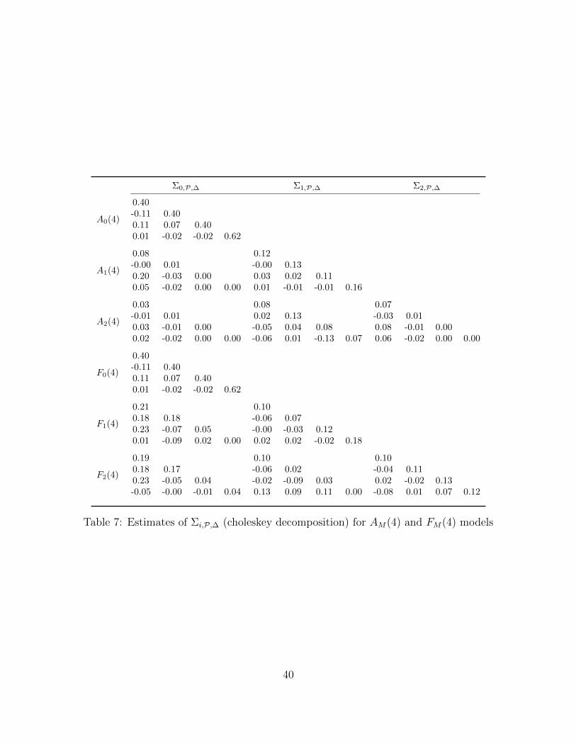
Σ0,P,∆ Σ1,P,∆ Σ2,P,∆

A0(4)

0.40-0.11 0.400.11 0.07 0.400.01 -0.02 -0.02 0.62

A1(4)

0.08 0.12-0.00 0.01 -0.00 0.130.20 -0.03 0.00 0.03 0.02 0.110.05 -0.02 0.00 0.00 0.01 -0.01 -0.01 0.16

A2(4)

0.03 0.08 0.07-0.01 0.01 0.02 0.13 -0.03 0.010.03 -0.01 0.00 -0.05 0.04 0.08 0.08 -0.01 0.000.02 -0.02 0.00 0.00 -0.06 0.01 -0.13 0.07 0.06 -0.02 0.00 0.00

F0(4)

0.40-0.11 0.400.11 0.07 0.400.01 -0.02 -0.02 0.62

F1(4)

0.21 0.100.18 0.18 -0.06 0.070.23 -0.07 0.05 -0.00 -0.03 0.120.01 -0.09 0.02 0.00 0.02 0.02 -0.02 0.18

F2(4)

0.19 0.10 0.100.18 0.17 -0.06 0.02 -0.04 0.110.23 -0.05 0.04 -0.02 -0.09 0.03 0.02 -0.02 0.13-0.05 -0.00 -0.01 0.04 0.13 0.09 0.11 0.00 -0.08 0.01 0.07 0.12

Table 7: Estimates of Σi,P,∆ (choleskey decomposition) for AM(4) and FM(4) models

40

Σ0,P,∆ Σ1,P,∆ Σ2,P,∆

A0(3)0.41-0.11 0.400.10 0.07 0.41

A1(3)0.10 0.090.07 0.00 -0.02 0.100.25 -0.03 0.00 0.01 0.00 0.08

A2(3)0.03 0.08 0.030.02 0.00 -0.03 0.09 0.02 0.000.07 -0.02 0.00 -0.02 -0.02 0.02 0.07 -0.01 0.00

F0(3)0.40-0.11 0.400.11 0.07 0.41

F1(3)0.19 0.140.23 0.11 -0.09 0.090.21 -0.17 0.06 0.01 -0.02 0.14

F2(3)0.09 0.03 0.090.02 0.03 0.05 0.01 -0.07 0.030.26 -0.02 0.06 0.01 -0.02 0.00 0.02 0.08 0.04

Table 8: Estimates of Σi,P,∆ (choleskey decomposition) for AM(3) and FM(3) models

41

References

Almeida, C., J. J. Graveline, and S. Joslin, 2011, “Do interest rate options contain informationabout excess returns?,” Journal of Econometrics.

Bikbov, R., and M. Chernov, 2009, “”Unspanned Stochastic Volatility in Affine Models:Evidence from Eurodollar Futures and Options,” Management Science.

Campbell, J., 1986, “A defense of the traditional hypotheses about the term structure ofinterest rates,” Journal of Finance.

Campbell, J., and R. Shiller, 1991, “Yield Spreads and Interest Rate Movements: A Bird’sEye View,” Review of Economic Studies, 58, 495–514.

Carr, P., X. Gabaix, and L. Wu, 2009, “Linearity-Generating Processes, Unspanned StochasticVolatility, and Interest-Rate Option Pricing,” Discussion paper, New York University.

Cheridito, R., D. Filipovic, and R. Kimmel, 2007, “Market Price of Risk Specifications forAffine Models: Theory and Evidence,” Journal of Financial Economics, 83, 123 – 170.

Chernov, M., and P. Mueller, 2009, “The Term Structure of Inflation Expectations,” Discussionpaper, London Business School.

Collin-Dufresne, P., R. Goldstein, and C. Jones, 2008, “Identification of Maximal Affine TermStructure Models,” Journal of Finance, LXIII, 743–795.

Collin-Dufresne, P., R. Goldstein, and C. Jones, 2009, “Can Interest Rate Volatility BeExtracted From the Cross Section of Bond Yields?,” Journal of Financial Economics, 94,47–66.

Collin-Dufresne, P., and R. S. Goldstein, 2002, “Do Bonds Span the Fixed Income Markets?Theory and Evidence for ‘Unspanned’ Stochastic Volatility,” Journal of Finance, 57,1685–1730.

Cox, J., J. Ingersoll, and S. Ross, 1985, “An Intertemporal General Equilibrium Model ofAsset Prices,” Econometrica, 53, 363–384.

Dai, Q., and K. Singleton, 2000, “Specification Analysis of Affine Term Structure Models,”Journal of Finance, 55, 1943–1978.

Dai, Q., and K. Singleton, 2002, “Expectations Puzzles, Time-Varying Risk Premia, andAffine Models of the Term Structure,” Journal of Financial Economics, 63, 415–441.

Dai, Q., and K. Singleton, 2003, “Term Structure Dynamics in Theory and Reality,” Reviewof Financial Studies, 16, 631–678.

de los Rios, A. D., 2013, “A New Linear Estimator for Gaussian Dynamic Term StructureModels,” Discussion paper, Bank of Canada.

42

Duarte, J., 2004, “Evaluating an Alternative Risk Preference in Affine Term Structure Models,”Review of Financial Studies, 17, 379–404.

Duffee, G., 2002, “Term Premia and Interest Rates Forecasts in Affine Models,” Journal ofFinance, 57, 405–443.

Duffee, G., 2011, “Forecasting with the Term Structure: the Role of No-Arbitrage,” Discussionpaper, Johns Hopkins University.

Duffie, D., D. Filipovic, and W. Schachermayer, 2003, “Affine Processes and Applications inFinance,” Annals of Applied Probability, 13, 984–1053.

Jacobs, K., and L. Karoui, 2009, “Conditional volatility in affine term-structure models:Evidence from Treasury and swap markets,” Journal of Financial Economics, 91, 288–318.

Joslin, S., 2013a, “Can Unspanned Stochastic Volatility Models Explain the Cross Section ofBond Volatilities?,” Discussion paper, USC.

Joslin, S., 2013b, “Pricing and Hedging Volatility in Fixed Income Markets,” Discussionpaper, Working Paper, USC.

Joslin, S., A. Le, and K. Singleton, 2012, “Why Gaussian Macro-Finance Term StructureModels Are (Nearly) Unconstrained Factor-VARs,” Journal of Financial Economics, forth-coming.

Joslin, S., K. Singleton, and H. Zhu, 2011, “A New Perspective on Gaussian DTSMs,” Reviewof Financial Studies.

Le, A., K. Singleton, and J. Dai, 2010, “Discrete-Time AffineQ Term Structure Models withGeneralized Market Prices of Risk,” Review of Financial Studies, 23, 2184–2227.

Litterman, R., J. Scheinkman, and L. Weiss, 1991, “Volatility and the Yield Curve,” Journalof Fixed Income, 1, 49–53.

Longstaff, F. A., and E. S. Schwartz, 1992, “Interest Rate Volatility and the Term Structure:A Two-Factor General Equilibrium Model,” Journal of Finance, 47, 1259–1282.

Piazzesi, M., 2010, “Affine Term Structure Models,” in Y. Ait-Sahalia, and L. Hansen (ed.),Handbook of Financial Econometrics . chap. 12, pp. 691–766, Elsevier B.V.

Trolle, A. B., and E. S. Schwartz, 2009, “A general stochastic volatility model for the pricingof interest rate derivatives,” Review of Financial Studies, 22, 2007–2057.

43