Interface Anisotropy and its Effect on

Microstructural Evolution During Coarsening

Tomoko Sano

Ph.D. Thesis

Materials Science and Engineering Department

Carnegie Mellon University

Pittsburgh, PA 15213

April 29, 2005

Thesis Committee:

Professor Gregory Rohrer (Advisor, Carnegie Mellon University)

Professor Martin Harmer (Lehigh University)

Professor Anthony Rollett (Carnegie Mellon University)

Professor Paul Salvador (Carnegie Mellon University)

Professor Paul Wynblatt (Carnegie Mellon University)

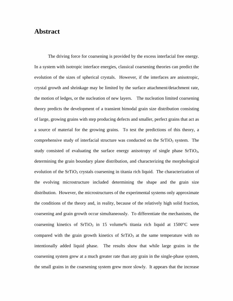
Abstract

The driving force for coarsening is provided by the excess interfacial free energy.

In a system with isotropic interface energies, classical coarsening theories can predict the

evolution of the sizes of spherical crystals. However, if the interfaces are anisotropic,

crystal growth and shrinkage may be limited by the surface attachment/detachment rate,

the motion of ledges, or the nucleation of new layers. The nucleation limited coarsening

theory predicts the development of a transient bimodal grain size distribution consisting

of large, growing grains with step producing defects and smaller, perfect grains that act as

a source of material for the growing grains. To test the predictions of this theory, a

comprehensive study of interfacial structure was conducted on the SrTiO3 system. The

study consisted of evaluating the surface energy anisotropy of single phase SrTiO3,

determining the grain boundary plane distribution, and characterizing the morphological

evolution of the SrTiO3 crystals coarsening in titania rich liquid. The characterization of

the evolving microstructure included determining the shape and the grain size

distribution. However, the microstructures of the experimental systems only approximate

the conditions of the theory and, in reality, because of the relatively high solid fraction,

coarsening and grain growth occur simultaneously. To differentiate the mechanisms, the

coarsening kinetics of SrTiO3 in 15 volume% titania rich liquid at 1500°C were

compared with the grain growth kinetics of SrTiO3 at the same temperature with no

intentionally added liquid phase. The results show that while large grains in the

coarsening system grew at a much greater rate than any grain in the single-phase system,

the small grains in the coarsening system grew more slowly. It appears that the increase

in the average size of the small grains can be attributed to grain growth rather than

coarsening. The simultaneous existence of a constant number of crystals that coarsen

rapidly and a decreasing number of small grains that grow only by grain boundary

migration is consistent with the nucleation limited coarsening theory.

Table of Contents

1. Introduction 1

1.1 Motivation…………………………………………………………. 1

1.2 Objectives and Approach………………………………………….. 4

1.3 References…………………………………………………………. 5

2. Background 7

2.1 Growth Phenomena………………………………………………… 7

2.2 Grain Growth………………………………………………………. 8

2.3 Classical Theory of Coarsening……………………………………. 8

2.4 Abnormal Coarsening……………………………………………… 10

2.5 Coarsening Mechanism……………………………………………. 13

2.5.1 Diffusion Limited Coarsening Mechanism……………….... 14

2.5.2 Surface Attachment Rate Limited Mechanism…………….. 17

2.5.3 Ledge Coarsening Mechanism…………………………….. 18

2.5.4 Nucleation Limited Coarsening……………………………. 21

2.6 Effect of Nucleation Energy Barrier on Coarsening……………….. 22

2.6.1 Effect of Surface Structure on Growth…………………….. 22

2.6.2 Growth by Two Dimensional Nucleation………………….. 28

2.6.3 Nucleation Limited Morphological Changes………………. 31

2.6.4 Effect of NEB on Coarsening……………………………….32

2.6.5 Experimental Evidence of the NEB…………………………37

2.7 System of Interest………………………………………………….. 40

i

2.8 References………………………………………………………….. 42

3. Microstructure Characterization Methods 48

3.1 Sample Preparation………………………………………………….48

3.1.1 Solid-Vapor Study Sample………………………………….48

3.1.2 Solid-Liquid Study Samples……………………………….. 49

3.1.3 Templated Single Crystal Samples………………………….53

3.2 Optical Microscopy…………………………………………………54

3.3 Atomic Force Microscopy…………………………………………..54

3.4 Orientation Imaging Microscopy……………………………………56

3.5 Scanning Electron Microscopy……………………………………..59

3.6 Analysis……………………………………………………………. 60

3.6.1 Measurement of Surface Energy Anisotropy……………….60

3.6.2 Coarsening Analysis……………………………………….. 67

3.7 Misorientation Averaged Distribution of SrTiO3 Grain Boundary

Planes………………………..……………………………………... 71

3.8 References………………………………………………………….. 72

4. SrTiO3 Solid-Vapor Surface Energy 75

4.1 Results……………………………………………………………… 75

4.2 Discussion………………………………………………………….. 85

4.3 References………………………………………………………….. 86

5. Grain Boundary Analysis 89

5.1 Orientation Distribution……………………………………………. 88

5.2 References………………………………………………………….. 90

ii

6. Grain Growth Experiments 91

6.1 Grain Size Distributions…………………………………………….91

6.2 Grain Growth Rate………………………………………………….92

6.3 References…………………………………………………………..94

7. Morphological Changes During Coarsening 95

7.1 Results……………………………………………………………… 95

7.2 Discussion…………………………………………………………..100

7.3 References………………………………………………………….. 103

8. Evolution of the Size Distribution During Coarsening 104

8.1 Crystal Shapes in Liquid…………………………………………… 104

8.2 Results of the Grain Population Based on Size……………………. 111

8.3 References………………………………………………………….. 117

9. Kinetics of Growth 118

9.1 Comparison with Grain Growth Rate……………………………….118

9.2 Calculated Small Grain Sizes………………………………………. 121

9.3 References………………………………………………………….. 123

10. Conclusions 125

11. Future Work 127

11.1 Monte Carlo Simulation …………………………………… ………127

11.2 Grain Boundary Wetting…………………………………………… 128

11.3 References………………………………………………………….. 128

Appendix A 130

Appendix B 140

iii

List of Figures

Fig. 2.1. The grain size distribution predicted by classical coarsening theory…….. 10

Fig. 2.2. Growth rate of uranium particles in lead………………………………… 11

Fig. 2.3. Average grain sizes of matrix grains annealed at 1350°C.………………. 13

Fig. 2.4. Comparison of theoretical interaction rate limited grain size distribution

functions………………………………...…………………….….…………16

Fig. 2.5. The effect of volume fraction of precipitates on Ardell’s grain size

distribution function……………………….……………………………….. 17

Fig. 2.6. The concentration gradient for surface attachment and diffusion

limited coarsening mechanisms………………………….………………….18

Fig. 2.7. Comparison of experimental to theoretical grain size…………….……… 19

Fig. 2.8. Interfacial ledge schematic of precipitate β in matrix α.…………..…….. 20

Fig. 2.9. (a) A rough surface. (b) A flat facet. ………………………………………21

Fig. 2.10. The Wulff construction…………………………………………………. 23

Fig. 2.11. The five possibilities of Wulff shapes...………………………………… 24-25

Fig. 2.12. The change of enthalpy and entropy at the interface …………………… 27

Fig. 2.13. The energy function ∆E plotted against………………………………... 35

Fig. 2.14. The nucleation energy barrier condition for dissolution or growth….….. 36

Fig. 2.15. Coarsening simulation of perfect and defective crystal populations…… 38

Fig. 2.16. (a) Initial sapphire crystals with cavities. (b) After 4h at 1900°C.

(c) After 16h at 1900°C …………………………………………………….40

iv

Fig. 3.1. Phase diagram of SrO-TiO2 system.……………………………………... 49

Fig. 3.2. SEM image of 20mole% TiO2 - 80mole% SrTiO3 powder………..…….. 50

Fig. 3.3. X-ray diffraction peaks from the 50 h sample…………………………… 50

Fig. 3.4. Backscattered electron image of the 10 h sample. (b) Image of the

eutectic precipitate…………………………………………………………. 51

Fig. 3.5. Optical image of an included SrTiO3 grain……………………………… 54

Fig. 3.6. AFM image of (a) an included grain and (b) a thermally grooved

grain boundary.…………………... ………………..……………………… 54

Fig. 3.7. A schematic of the orientation imaging microscope…………………….. 55

Fig. 3.8. An EBSP (Kikuchi pattern) of a SrTiO3 crystal…………………………. 56

Fig. 3.9. Transformation from the sample to the crystal coordinate system…….… 57

Fig. 3.10. An inverse pole figure map of a SrTiO3-TiO2…………………………. 58

Fig. 3.11. A schematic of a thermal groove……………………………………….. 60

Fig. 3.12. Schematics of a thermally grooved triple junction……………………... 61

Fig. 3.13. Schematic of an included grain……………………………….…………63

Fig. 3.14. (a) Optical images of an included grain the first and second layer,

and (b) a schematic of the included grains…………………………………. 64

Fig. 3.15. A planar AFM image of grains coarsened at 1500°C for 24 h…...…….. 66

Fig. 3.16. (a) The habit planes for line segment lij. (b) The stereographic pro-

jection of nijk and line lij. ……………..……………………………………. 68

Fig. 3.17. A schematic of , angle θijlr

k, and normals . ………………………... 68 ijkn

Fig. 3.18. Discretized quarter of the orientation space…………………………….. 69

Fig. 3.19. Correct habit plane normals become evident with more traces………… 70

v

Fig. 4.1. Three examples of the ln(w) vs. ln(t) relations………………….……….. 75

Fig. 4.2. An example of a thermal groove trace…………………………………… 76

Fig. 4.3. Surface normal observations plotted in the SST…………………………. 77

Fig. 4.4. Stereographic projection of the surface energies………………………… 78

Fig. 4.5. The plot of discrete surface energy data and the Fourier series fit.………. 79

Fig. 4.6. Deviations from ideal behavior, plotted for all orientations……………... 80

Fig. 4.7. (a). SST of faceted and non-faceted orientations. (b) A surface

bounded by two facets. (c) A surface bounded by three facets………….….81

Fig. 4.8. Equilibrium crystal shape of SrTiO3 at 1400°C in air……………………. 84

Fig. 5.1. (a) Misorientation averaged distribution of grain boundary planes.

(b) Surface energy projection……………………………….……………… 88

Fig. 5.2. Grain boundary population as a function of surface energies…………… 90

Fig. 6.1. SEM image of the 24 h sample……………………………………………91

Fig. 6.2. Log normal distribution and the grain size distribution plotted for (a) 0 h,

(b) 5 h, (c) 10 h, (d) 15 h, and (e) 24 h samples……………………………. 93

Fig. 6.3. Average grain size over time…………………………………………….. 94

Fig. 7.1. AFM images of (a) 0 h sample and (b) 24 h sample…………………….. 95

Fig. 7.2. (a) Distribution of SrTiO3 interfaces for the 0 h sample, and (b) 24 h

sample. Both determined by manual boundary tracing…………………….97

Fig. 7.3. The reconstructed boundary image of the 10h sample…………………... 98

Fig. 7.4. Automatic extraction of grain boundaries from the OIM images. (a)

Distribution of SrTiO3 interfaces for the 5 h sample. (b) Distribution of

SrTiO3 interfaces for the 10 h sample. (c) Distribution of SrTiO3

vi

interfaces for the 24 h sample……………………………………………… 99

Fig. 7.5. (a) an OIM map of the templated (111) single crystal. (b) An OIM map

of a templated (100) single crystal…………………………………………. 102

Fig. 8.1. (a) An SEM image of the 0 h anneal sample, (b) 5 h annealed sample,

(c) 10 h anneal sample, and (d) 50 h annealed sample……………. ………105

Fig. 8.2. Frequency of grain sizes for the 24 h solid-liquid sample compared to

the LSW distribution…………………………………………….…………. 107

Fig. 8.3. Frequency of grain size versus the normalized grain size for solid-liquid

samples annealed for (a) 0 h, (b) 3 h, (c) 5 h, (d) 10 h, (e) 15 h, (f) 24 h, and

(g) 50 h……………………………………………………………………... 108

Fig. 8.4. Grain size distribution of solid-liquid samples annealed for (a) 0 h, (b) 3 h,

(c) 5 h, (d) 10 h, (e) 15 h, (f) 24 h, and (g) 50 h…………………………... 109

Fig. 8.5. (a) Volume percentages of 5 h grain growth sample compared with

classical grain growth theory (b) Volume percentages of the 5h coarsening

sample compared with LSW….……………………………………………. 110

Fig. 8.6. The median abnormal grain size over time……………………………….112

Fig. 8.7. Volume density of abnormal grains versus annealing time…………….... 113

Fig. 8.8. The sizes of the small grains versus time…………………………………115

Fig. 8.9. Small grain size results compared to small grains size results by Rehrig.. 116

Fig. 8.10. Volume density of small grains versus time……………………………. 116

Fig. 9.1. Grain growth rate versus coarsening rates……………………………….. 120

Fig. 9.2. Experimental and calculated small grain sizes over time…………………122

vii

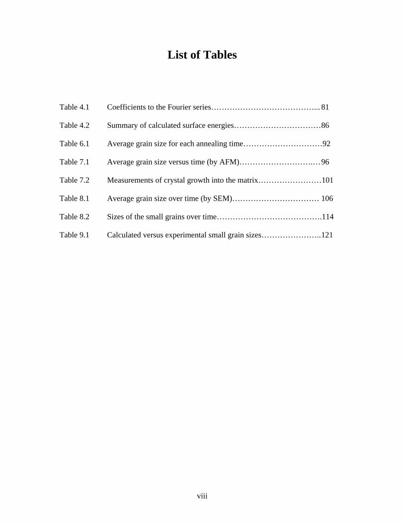
List of Tables

Table 4.1 Coefficients to the Fourier series…………………………………... 81

Table 4.2 Summary of calculated surface energies…………………………… 86

Table 6.1 Average grain size for each annealing time…………………………92

Table 7.1 Average grain size versus time (by AFM)……………………….… 96

Table 7.2 Measurements of crystal growth into the matrix……………………101

Table 8.1 Average grain size over time (by SEM)…………………………… 106

Table 8.2 Sizes of the small grains over time………………………………….114

Table 9.1 Calculated versus experimental small grain sizes………………….. 121

viii

List of Variables

c∞ Far field molar concentration

cR Equilibrium concentration at the phase boundary

r Radius

K Rate constant

γ Surface / interface energy

T Temperature

k Boltzmann’s constant

v Atomic volume

j Atomic flux

D Diffusion coefficient

∆ Supersaturation value

r* Critical radius

ρ Ratio of r to r*

A Constant

r Average grain size

α α = 2γvc∞ / kT

Ω Molar volume

ce Molar concentration of solute

t Time

R Gas constant

f(φ) Volume fraction relation

w Constant or function

cm Concentration of the matrix

L Cube length βBx Mole fraction of solute B in β precipitate

αBx Mole fraction of solute B in α matrix

ϖ Function that evaluate diffusion field

ix

λ Ledge separation distance

L Average ledge length

E Total surface energy

n Normal orientation

S Surface of the Crystal

ri Radius to surface i

s Number of atoms

∆G Free energy change

δ Supersaturation factor

ϕ Nearest neighbor interaction bond energy

ω Nucleus size

AF Facet area

a Atomic height

µe Chemical potential of the reservoir

µs Chemical potential of the crystal surface

µ∞ Chemical potential far from the particle

µeq Equilibrium chemical potential

rc Cube radius

ξ Ratio of µs to µ∞I Nucleation rate

C C = Znmg

Z Zeldovich factor

nm Density of monomers at the facet

g Rate at which critical nuclei becomes supercritical

E+ Energy barrier for addition of atoms

E- Energy barrier for removal of atoms

diffR& Rate of particle coarsening by diffusion

nucR& Rate of particle coarsening by nucleation

n Normal vector

W Groove width

x

χi Half dihedral angle

Ψ Dihedral angle

N Number of diffusing species

φ1 First Euler angle

Φ Second Euler angle

φ2 Third Euler angle

angle α Grain boundary inclination

angle β Right-hand rotation about l

angle τ In-plane angle

l Line of intersection of interfaces

H Height

θ, ϕ Spherical angles iξv

Cahn-Hoffman capillarity vector

pr Probability function

λ(n) Surface normal distribution

λ(∆g,n) Grain boundary distribution

∆g Misorientation

p Pauling’s electrostatic bond valence

p1 Fitting parameter 1 for log normal function

p2 Fitting parameter 2 for log normal function

Nv Volume density of grains

NA Area density of grains

d Grain diameter

xi

1. Introduction

1.1 Motivation

Grain growth is the process in which the average size of the crystals in a dense

polycrystal increases. Since volume must be conserved, this means that some grains

grow while others shrink. If this occurs in a system where a second phase intervenes

between the grains, it is referred to as coarsening or Ostwald ripening. In both cases, the

driving force for the increase in the average grain size is the interfacial energy. As the

average size of the crystals in the system increases, the total interfacial area (and the

associated energy) decreases.

The classical theory of coarsening, established by Lifshitz, Slyozov1 and Wagner2

(LSW), assumes that the coarsening phase is infinitely dilute, so that the average

chemical potential surrounding each crystal is the same. This mean field chemical

potential, µ*, establishes a characteristic size, r* = 2γ/µ* (where γ is the surface energy

per unit area), for a crystal that neither shrinks nor grows. Crystals larger than the critical

radius, r*, grow while those smaller than r* shrink. The theory predicts that the average

radius increases with time raised to the power n, where n = 1/3 for diffusion limited

growth and n = 1/2 for surface attachment limited growth. The theory also predicts a

time independent distribution of normalized grain sizes with the largest grain size being

approximately 3/2 times the average radius. While the LSW theory is in qualitative

agreement with experimental observations, many of the details are quantitatively

1

incorrect. For example, observed grain size distributions are usually different and the

maximum grain size is almost always larger than the predicted size.

The limits of LSW theory are best illustrated by processes where abnormal

coarsening is used to control texture or microstructure. For example, in the templated

grain growth (TGG) process, large seeds are combined with a matrix of much finer grains

of the same size. Interestingly, the larger seeds grow at rates more than an order of

magnitude faster than the matrix grains. While it is true that the large grains enjoy a

small advantage in the capillary driving force, this cannot explain the difference in the

growth rates. In general, the LSW theory provides no explanation for the occurrence and

persistence of bimodal grain size distributions that occur frequently in coarsening

systems of crystals with anisotropic surface energies.

Although the mechanism of abnormal coarsening is not yet understood, it remains

as a useful procedure for growing single crystals of phases that cannot be obtained by

traditional methods. For example, if a phase melts incongruently, or if it undergoes a

phase change after solidification, the only option is to grow the material from a lower

temperature flux. It has been found that large crystals can be grown in seeded

polycrystalline compacts with only a small amount of liquid flux present. This method

has been used on an industrial scale to grow single crystal ferrites to be used as recording

heads in video cassette recorders3. General Electric Co. also uses sapphire seed crystals

in polycrystalline alumina to convert polycrystalline bodies to sapphire single crystals4.

Using single crystal sapphire arc tubes prolongs the life of high-pressure sodium arc

discharge lamps. TGG is also used to grow piezoelectric ceramics used in transducers

and sensors for industrial and military applications5, 6.

2

As mentioned above, the accelerated growth rate of certain seeds is not yet

explained. Kang et al.7 and Chung et al.8, 9 have suggested that abnormal grain growth

occurs by the twin-plane reentrant edge mechanism. They argue that the locations of

twin plane reentrant edges are favorable attachment sites for precipitates, and hence these

grains grow abnormally. However it is unclear if the abnormal growth is because of the

existence of twins, or the twins are simply a highly probable defect in very large grains.

If abnormal growth occurs only for grains with twins, it does not explain the existence of

abnormal SrTiO3 grains that do not have twins. The abnormal coarsening of SrTiO3 will

be described in later chapters.

To understand other reasons for accelerated growth, one can begin by examining

some of the assumptions of LSW theory to identify potential weaknesses. While

abnormal coarsening is usually observed in systems with a high volume fraction of solid,

LSW assumes infinite dilution. Another assumption of LSW theory is that the surface

energies are isotropic, while abnormal coarsening is most frequently observed in systems

that have anisotropic surface energies. Surface energy anisotropy can have several

effects. First, it complicates the driving forces for coarsening, which will vary not only

with the size of the crystals, but also with the shape. The second is that it can lead to the

formation of singular surfaces, where the nucleation of new ledges may become the rate-

limiting factor in growth. Recent simulations have substantiated the hypothesis that

defect controlled growth in a nucleation limited situation can lead to bimodal grain size

distributions10. At this time, however, the experimental support for this theory is not

conclusive.

3

1.2. Objectives and Approach

The hypothesis of this work is that a coarsening theory that incorporates surface

energy anisotropies and the influence of interface structure on the growth mechanism will

be able to explain abnormal coarsening. Simulations based on these ideas are already

available10. The missing component is a rigorous comparison to experimental

observations. Therefore, the central objective of this thesis is to accumulate the

necessary data and compare the results to the predictions of the simulations.

To test this hypothesis, it will be necessary to have comprehensive microstructural

data at various stages of growth and to understand the anisotropy of the interfacial

energy. However it is impossible to create a sample that mimics the microstructure

considered in the nucleation limited coarsening theory. High liquid volume fractions are

not practical because of sedimentation of the solid, which leads to impingement. With

minimized volume fraction of liquid, grains will once again impinge upon each other.

These grains will evolve by two mechanisms: grain growth and coarsening. Hence the

experimental portion of this thesis will have two parts. The first part will address the

grain growth aspect of the microstructural evolution. The second part will address the

combined coarsening and grain growth process in solid-liquid compacts with finite liquid

fractions.

By quantifying the grain growth rates and grain sizes from the grain growth

experiments of single-phase samples, we will attempt to separate out the grain growth

effects from the combined coarsening and grain growth sample to determine the

coarsening mechanism.

4

For this thesis, the combined coarsening and grain growth work will concentrate

on SrTiO3 excess TiO2. At elevated temperatures, solid SrTiO3 is in equilibrium with a

TiO2 rich liquid. This system is relatively well understood and it exhibits abnormal

growth phenomena. As part of the present work, the anisotropy of the surface energy has

been studied in air. Interface distributions have also been measured in both the dense

polycrystal and the solid liquid system and qualitative aspects of the grain boundary and

surface-liquid anisotropy can be inferred. Finally, the distributions of grain sizes and

shapes have been measured as a function of time. The final step of the thesis will be to

evaluate these data with respect to grain growth, classical coarsening, and defect

controlled coarsening models.

1.3 References

1. I. M. Lifshitz, and V. V. Slyozov, “The Kinetics of Precipitation From

Supersaturated Solid Solutions,” J. Phys. Chem. Solids, 19 [1/2] 33-40 (1961).

2. C. Wagner, “Theorie der Alterung von Niederschlägen durch Umlösen (Ostwald-

Reifung),” Z. Elektrochemie, 65 [7/8] 581-591 (1961).

3. S. Matsuzawa and S. Mase, “Method for Producing a Single Crystal of Ferrite”

U.S. Patent 4339301 (1982).

4. C. E. Scott, J. M. Strok, L.M. Levinson, “Solid State Thermal Conversion of

Polycrystalline Alumina to Sapphire Using a Seed Crystal” U.S. Patent 5549746

(1996).

5. G. S. Rohrer, C. L. Rohrer, and W. W. Mullins, “Coarsening of Faceted Crystals,”

J. Am. Ceram. Soc. 85 [3] 675-682 (2002).

5

6. M. P. Harmer, H. M. Chan, H.-Y. Lee, A. M. Scotch, T. Li, F. Meschke, and A.

Khan, “Method for Growing Single Crystals from Polycrystalline Precursors,”

U.S. Pat. No. 6 048 394, 2000.

7. M.-K. Kang, Y.-S. Yoo, D.-T. Kim, and N. M. Hwang, “Growth of BaTiO3 Seed

Grains by the Twin-Plane Reentrant Edge Mechanism,” J. Am. Ceram. Soc. 83 [2]

385-390 (2000).

8. U.-J. Chung, J.-K. Park, N.-.M. Hwang, H.-Y. Lee, and D.-Y. Kim, “Effect of

Grain Coalescence on the Abnormal Grain Growth of Pb(Mg1/3Nb2/3)O3-35 mol%

PbTiO3 Ceramics,” J. Am. Ceram. Soc. 85 [4] 965-968 (2002).

9. U.-J. Chung, J.-K. Park, N.-.M. Hwang, H.-Y. Lee, and D.-Y. Kim, “Abnormal

Grain Growth of Pb(Mg1/3Nb2/3)O3-35 mol% PbTiO3 Ceramics Induced by the

Penetration Twin,” J. Am. Ceram. Soc. 85 [12] 3076-3080 (2002).

10. G. S. Rohrer, C. L. Rohrer, and W. W. Mullins, “Coarsening of Faceted Crystals,”

J. Am. Ceram. Soc., 85 [3] 675-682 (2002).

6

2. Background

2.1 Growth Phenomena

There are several related processes in which the crystals in a microstructure

increase their average size with time. These are grain growth, liquid phase sintering, and

coarsening. While these terms are frequently used interchangeably, the following

definitions will be used in this thesis.

Grain growth occurs in an entirely solid system. Here the transfer of atoms across

the interface is the elementary process by which boundaries move. Liquid phase

sintering is a process in which solid grains are consolidated in the presence of a liquid

phase. The composition of the sample is selected so that solid and liquid phases coexist

when heated to high temperatures. As long as the solid-liquid surface energy is low,

many of the boundaries will be wetted by the liquid, which assists with both the

densification of the powder and the transport of dissolved atoms toward growing grains

and away from shrinking grains. In liquid phase sintering, the elementary process is the

dissolution of material from one crystal, its diffusion through the liquid, and precipitation

on another grain. In liquid phase sintering, the volume fraction of the liquid phase is

usually minimized. If the volume fraction of the intervening phase is larger than the

minimum required to wet all of the grain boundaries, or the system has proceeded beyond

densification to the growth stage, it will be referred to as coarsening. However it should

be noted that liquid phase sintering and coarsening cannot occur independently of grain

growth. In both of the cases where liquid is present, boundaries between impinging

7

crystals can move and grain growth can occur. This is an important consideration in the

interpretation of the experiments in this thesis.

According to these definitions, this thesis is about both grain growth and

coarsening. Specifically the role of both mechanisms in the case of a solid phase in the

presence of a liquid is considered. Grain growth and the classical theory of coarsening

are described in the next section.

2.2 Grain Growth

Normal grain growth occurs when a dense, single-phase polycrystalline sample is

annealed. The driving force for growth is the reduction of the total interface energy. The

grain size distribution of the sample is said to be self-similar, and has been reported to be

lognormal1, 2. The average grain size, r , follows the relation3,

( )nKtrr =− 0 , (2.1)

where 0r is the initial average grain size, K is a constant, and the exponent n is ideally ½.

Most experimental measurements yield exponents less than ½, due to impurities and

pores.

2.3 Classical Theory of Coarsening

The classical theory of coarsening was written by Lifshitz, Slyozov4, and Wagner5

(LSW). They found after the characteristics of the initial state are erased, the average

size of the particles in a saturated solution increases with time to the 1/3 power. The

theory simplifies the situation by assuming the solid phase occupies a minimal volume

fraction of the system. The solid is also assumed to have isotropic surface energies.

8

These two assumptions make it possible to assume each particle is embedded in a

medium with a uniform far field molar concentration, (c∞), so that the equilibrium

concentration, (cR), at the phase boundary of the spherical particles of radius r can be

expressed by the Gibbs-Thomson relation,

∞∞ ⎟⎠⎞

⎜⎝⎛+= c

kTv

rccR

γ2 (2.2)

where γ is the interface energy, T is temperature, k is the Boltzmann’s constant, and v is

the atomic volume of the solute. Eq. (2.2) implies that there are crystals with a critical

size that are in equilibrium with the solution; crystals smaller than this radius are not

stable and will dissolve in the solution while those that are larger will act as substrates for

the precipitation of material from the solution.

The diffusive flux of solute atoms across the phase boundary per unit area is

based on Fick’s first law and is given as,

( ) ⎟⎠⎞

⎜⎝⎛ −∆=−=

∂∂

== rr

DccrD

rCDj R

Rr

α , (2.3)

where the term α = (2γ/kT)vc∞ consolidates the variables in Eq. (2.2). Since the atomic

flux, j, makes the crystal grow or shrink, this is equal to the time rate of change of the

crystal radius, dr/dt. For every supersaturation value ∆, which is the difference c-c∞,

there exists a critical radius of a grain, r* = α/∆, which is in equilibrium with the solution.

If the radius r of a grain is greater than r*, the grain will grow. If r is less than r*, the

grain will dissolve. Using this as a basis, it was determined that the average grain size

follows the relation,

31

94

⎟⎠⎞

⎜⎝⎛= tDr α . (2.4)

9

The time independent part of the grain size distribution function, F(ρ) is

dependent on the normalized radius value ρ, defined as ρ = r / r*.

⎥⎥

⎦

⎤

⎢⎢

⎣

⎡

−

−⎟⎟⎟

⎠

⎞

⎜⎜⎜

⎝

⎛

−⎟⎟⎠

⎞⎜⎜⎝

⎛+

=ρ

ρρρ

ρρ2

3exp

23

23

33)(

311

37

2AF , (2.5)

where A is a constant. With this grain size distribution, the maximum grain size is

approximately 3/2ρ (see Fig. 2.1).

2.4. Abnormal Coarsening

Abnormal coarsening is when a minority subset of grains in the system grows at a

0.0

0.5

1.0

1.5

2.0

2.5

0.0 0.5 1.0 1.5 2ρ

F(ρ)

.0

Fig. 2.1. The grain size distribution predicted by classical coarsening theory4, 5. See Eq. (2.5).

10

greater rate than the other crystals. The distribution of the grain sizes in this case is

bimodal. The mechanism of abnormal coarsening is not understood but second phase

particles, liquid phases, and crystal defects have been implicated6. Considering that the

growth rate depends on the inverse of the grain radius, abnormal growth is kinetically

unfavorable. In other words, larger grains should grow more slowly than smaller ones.

For example, Fig. 2.2 shows the growth rate of uranium grains in lead at 750°C for

different average grain sizes7. The interesting and unexplained aspect of abnormal

growth is that some grains somehow grow several times larger than the average grain size

even though they are expected to have growth rates less than the smaller grains. In this

thesis, the analysis of the experimental data will consider grains in the first peak of the

bimodal grain size distribution as “small” grains and grains in the second peak at larger

grain sizes as “abnormal” grains. The abnormal grain categorization was found to be

-6-4-202468

101214

0 20 40 60 8

Particle Radius (µm)

Gro

wth

Rat

e dR

/dt (

µm/d

ay)

mean R = 5 µm

mean R = 10 µm

mean R = 20 µm

0

Fig. 2.2. Growth rate of uranium particles in lead, with different average grain sizes at 750°C7.

11

beyond the maximum grain size expected by LSW (3/2ρ), and beyond that predicted by

other theories, described in Section 2.5.

Abnormal coarsening has been used to grow single crystals in a controlled manner

by the solid state crystal conversion and templated grain growth (TGG) techniques. The

technique used to coarsen a single crystal abnormally is called solid state crystal

conversion (SSCC). A single crystal is embedded in a powder compact and is sintered

and annealed. The single crystal will grow into the polycrystalline matrix, which has a

small amount of liquid phase. This technique has been used to grow Pb(Mg1/3Nb2/3)O3 -

35mol%PbTiO3 (PMN-35PT) and is very similar TGG 8-10.

TGG is a method often used to grow large single crystals. The difference

between TGG and SSCC is that TGG coarsens crystals with orientation control. Several

“template” seed crystals in alignment are embedded in a matrix. The matrix often starts

as a powder compact of polycrystals in a second phase. The compacted powder with the

seed crystals is sintered and annealed to grow the crystals. The seed grains will grow in

an exaggerated, anisotropic manner into the matrix, with preferences for certain

directions. Once the seed grains form faceted habit planes and impinge on other seed

crystals, the coarsening rate slows down10. This technique has been successfully used

with BaTiO3 and α-alumina11, 12.

A clear example of anisotropic abnormal coarsening is described in the paper by

Rehrig et al.11. In their study, they coarsened an abnormal BaTiO3 grain by TGG at

1350°C. They found that the single seed crystals grew in an anisotropic manner. The

111 surfaces moved at a rate an order of magnitude greater than that of 110 surfaces.

The velocity of the 111 orientation was roughly 590 µm/h but the 110 surface had a

12

0

1

10

100

1000

0 5 10 15 20 25 30 35Time (hours)

Ave

rage

Gra

in S

ize

( µm

)Fine GrainsExaggerated Grains

Fig. 2.3. Average grain sizes of matrix grains annealed at 1350°C. The values in the parentheses are the volume percentages of the exaggerated grains11.

(>95%) (~19%)(~6%)

(<1%)

velocity of 40 µm/h. The same trend was observed with a different matrix composition.

In addition, the sizes of these template crystals were a hundred times greater than the

sizes of the matrix grains. The matrix grains were also found to grow abnormally. Fig.

2.3 shows the average grain size of matrix grains as a function of annealing time at

1350°C 11. From 8 to 20 hours of annealing, there was a bimodal distribution of grain

sizes. After annealing for more than 32 hours, the matrix grain size ranged from 100 to

300 µm.

2.5. Coarsening Mechanism

The rate at which crystals coarsen can be controlled by the rate of diffusion, the

rate at which atoms attach to the surface, the rate at which ledges move on the surface, or

13

the rate at which new ledges nucleate on the surface. The influences of the different

mechanisms on coarsening are described below. There are four major mechanisms of

coarsening. They are diffusion limited, surface attachment rate limited, the ledge

mechanism, and nucleation limited mechanisms. Each will be explained in detail.

2.5.1 Diffusion Limited Coarsening Mechanism

Zener’s13 theory for diffusion controlled growth of precipitates preceded the LSW

theory (described in Section 2.3) by many years. However, Zener did not consider

curvature effects on the solute concentration and driving force. As a result, he arrived at

a parabolic growth law. Today, the LSW theory for diffusion controlled growth, which

predicts that the crystal size increases with time to the 1/3 power, is accepted.

Over the years, there have been several refinements to the diffusion limited

coarsening theory. For example, Lifshitz and Slyozov consider situations where crystals

grow by coalesence. This is a first order attempt to model coarsening in non zero volume

fractions, which will be described below. When particles are coarsening, they may come

into physical contact. When two particles come across each other, the larger particle will

consume the smaller particle, and it is assumed that the volume is conserved. For these

cases, Lifshitz and Slyozov use an “encounter integral” to modify the distribution. This

function incorporates the frequency of encounters of particles of various sizes. By

including particle encounters, the resulting size distribution function is broadened and the

peak is lowered.

Ardell14, Brailsford and Wynblatt15, Davies et al.16 and others17-19 have

incorporated the volume fraction of precipitates into LSW theory. The LSW theory does

14

not take volume fraction into account, hence is only valid for zero or very minimal

volume fraction of precipitates. In other words, the mean particle size is small compared

to the mean distance between particles. It was presumed that the coarsening rate would

increase with increasing volume fraction. If there are more particles in the matrix, the

mean distance between particles decreases, and the kinetics are altered due to the

decrease in the diffusion distance. With a large enough volume fraction, the mechanism

of coarsening will change to that of particle encounters.

Ardell14 incorporates the effects of volume fraction by altering LSW’s diffusion

geometry, and thus the kinetic equation. He describes the radius of constant solute

concentration around a spherical particle polydispersed in a medium. He relates the

radius of the region to the volume fraction and this affects the coarsening rate equation.

Brailsford and Wynblatt15 also modify the kinetic equation, but assume

homogeneous loss/gain of solute atoms in the medium. The solute loss and production

rate is based on the model of a spherical cavity filled with matrix material, surrounding a

spherical particle. The volume fraction of precipitate is related to the sizes of the cavity

and the particle. However, particle coalescence is neglected in their model.

Davies et al.16, differs from Ardell14 and Brailsford and Wynblatt15, in that they

only consider encounters of particles. Davies et al. assume that when a growing particle

encounters another particle, there is rapid transfer of material, and the two particles

coalesce into one. The idea is the same as LSW’s rate equation with particle encounters,

but the difference is that the volume fraction affects the rate constant and the particle size

distribution.

15

Although the previous coarsening rate models differ in approach, the rate

equations are similar. They take the form,

)(63

03 φ

γf

RTDtc

rr e ⋅Ω

=− , (2.6)

where γ is the interfacial energy, Ω is the molar volume of precipitate, ce is the moles per

volume of solute, D is the coefficient of solute diffusion, t is time, R is the gas constant, T

is temperature, and f(φ) is the volume fraction relation. In Ardell’s case, the f(φ) is a

complex relation of volume fraction of precipitates to particle radius. For both Brailsford

and Wynblatt, and Davies et al., f(φ) is ,1*

3

⎟⎠⎞

⎜⎝⎛⋅⎟⎟

⎠

⎞⎜⎜⎝

⎛wr

r where w is a constant for Brailsford

and Wynblatt, and a function of r* and r*0 for Davies et al. The models all produce

similar grain size distributions and the asymptotic results are shown in Fig. 2.414, 15, 16. A

0.0

0.2

0.4

0.6

0.8

1.0

1.2

1.4

1.6

0.0 0.5 1.0 1.5 2.0 2.5

R/R.average

Gra

in S

ize

Dis

trib

utio

n

Ardell

Brailsford andWynblattDavies et al.

Fig. 2.4. Comparison of theoretical interaction rate limited grain size distribution functions for precipitate volume fraction of 0.814, 15, 16.

16

0.0

0.5

1.0

1.5

2.0

2.5

0.0 0.5 1.0 1.5 2.0

R/R.average

Gra

in S

ize

Dis

trib

utio

n1%

0.05%

0%

Fig. 2.5. The effect of volume fraction of precipitates on Ardell’s grain size distribution function14.

comparison of the effect of the volume fraction of precipitates on the distribution is

shown in Fig. 2.514. In general, it can be said that as the particles become closer, the

grain size distribution broadens.

2.5.2 Surface Attachment Rate Limited Mechanism

In Section 2.5.1, the diffusion limited coarsening mechanism was described. In

that mechanism, the diffusion step was slow, but the reaction of the atoms to attach to the

surface of the crystal was fast. In the surface attachment/detachment rate limiting

kinetics (SALK), the opposite is true. The diffusion step is fast, but reaction at the

surface is slow. This is also referred to as a first order reaction limited mechanism.

While the diffusion limited coarsening mechanism had an increasing concentration

17

gradient of solute atoms from the bulk to the surface of a growing crystal, there is no

solute concentration gradient in this case, and concentration of the matrix, cm is a

horizontal line as shown in the plot in Fig. 2.621. Wagner5 was the first to determine that

the SALK coarsening rate is parabolic. This rate equation in terms of average particle

size and anneal time is, 2/1tr ∝ . The grain size distribution function for SALK was

determined by Wagner5 to be,

Fig. 2.6. The concentration gradient of solute atoms for surface attachment limited kinetics versus the diffusion limited coarsening mechanisms. Cm is the matrix concentration and cR is the equilibrium concentration at the surface of the crystal21.

Distance R Crystal surface

cR

cm SALK

Diffusion Limited

⎥⎦

⎤⎢⎣

⎡−

−⎟⎟⎠

⎞⎜⎜⎝

⎛−

=ρρ

ρρ

23exp

22)(

5

F , (2.7)

where time is constant. A comparison of the grain size distribution functions for the

different limiting mechanisms for coarsening is shown in Fig. 2.720, 21.

18

0.0

0.5

1.0

1.5

2.0

2.5

0.00 0.50 1.00 1.50 2.00 2.50R/R.average

F(R

/R.a

vera

ge)

LSW

LSW Vol.Fraction=0.8SALK

Exp. fitted curve

Fig. 2.7. Comparison of experimental grain size distribution of Ni3Al cubes coarsening in Ni-Al alloys, to theoretical LSW with encounters, and volume diffusion limited functions20, 21.

2.5.3 Ledge Coarsening Mechanism

The ledge coarsening mechanism has been considered for the case when the

diffusion rate and the surface attachment rates are comparable. Shiflet, Aaronson, and

Courtney20 modeled the ledge limited theory by considering coarsening cubes. They

assumed that the surfaces of the cubes migrated only by the ledge mechanism. The ledge

mechanism specifies that the interfaces have partially coherent stepped surfaces. They

found that the ledge mechanism kinetics were comparable to that of LSW. A schematic

of the ledge growth is shown in Fig. 2.8. The β phase particle will grow in the G

direction by atomic addition on the ledges, effectively “moving” the ledge in the direction

perpendicular to G, with velocity v. They determined that the average ledge length, L ,

19

varied as t1/3 for large particles and as t1/2 for small particles. Their model is based on a

situation where coarsening occurs only by particles attaching or detaching at surface

ledge sites. A schematic of the rough surface in comparison to a flat, singular surface is

shown in Fig. 2.9. They first determine the equation of the flux of atoms to or from the

matrix, and the equation for the flux of solute due to the growth of a cube. By equating

these two flux relations, the rate of growth dtdLL , for a single cube of precipitate of edge

length, L, was determined to be,

⎟⎠⎞

⎜⎝⎛ −

Ω−

−=LL

RTxxDx

dtdLL

BB

B 1)(

8ϖλγ β

αβ

α

. (2.8)

The variables and are the mole fraction of solute B in the β precipitate and

mole fraction in the α matrix, respectively. The variable D is the diffusivity, γ is the

interfacial energy of the cube, Ω is the molar volume, ω is a non-analytic function which

evaluates the diffusion field around the risers of the ledges, λ is the ledge separation,

βBx α

Bx

L

is the average edge length and RT has its usual meaning. If ϖ was independent of particle

Fig. 2.8. Interfacial ledge schematic of precipitate β in matrix α. The ledges have height h, moves at a velocity v, and are separated from the next ledge by a distance λ. Phase β will grow in the G direction.

vG

β phase

α phase

λ

h

20

(a) (b)

Fig. 2.9. (a) A rough surface with kinks that provide attachment and removal sites. (b) A flat facet with no preferential sites.

size, the integrated form of the rate equation becomes,

( ) ( )RTxx

tDxLLBB

B

ϖλγ

αβ

α

)(812562

02

−Ω

=− . (2.9)

However, ϖ describes the amount of the diffusion about the ledges, thus varies linearly

with particle size. The larger the particle, the larger the parameter ϖ will be. Taking this

linear relationship and applying it to Eq. (2.8) and integrating will give the relation of t ∝

3L for large particles. The resulting equation is,

( ) ( )RTxx

tDxALLBB

B

λγαβ

α

)()(3

03

−Ω

=− (2.10)

where A is a constant. Interestingly, Eq. (2.10) resembles Eq. (2.6), even though they

were constructed from different mechanisms.

21

2.5.4 Nucleation Limited Coarsening

The theories described in Sections 2.3, 2.5.1, 2.5.2 and 2.5.3, all assume that

atomic attachment and detachment sites are always present on the surface. If the surface

is flat and hence lacks these sites, then it will be necessary to create a ledge, and this will

require energy. Depending on the conditions, the required energy may be larger than

thermal fluctuations and if this is the case, the nucleation of new ledges will limit the rate

of coarsening. The following section is devoted to the discussion of nucleation limited

coarsening.

2.6. Effect of Nucleation Energy Barrier on Coarsening

When a single atom from vapor or liquid, attaches to a flat solid surface, the

associated increase in the interfacial energy prevents it from being energetically stable.

Therefore, it is likely to desorb and go back into the liquid or gas phase. This situation

can be remedied if there were a large number of single atoms coming together on the

surface, for example, in a supersaturated medium, so that the energy liberated by

crystallization is greater than the added interfacial energy. The energy required to

nucleate a step-edge on a flat surface that does not have attachment or detachment sites is

referred to as the nucleation energy barrier. In this section, the influence of surface

structure on growth, nucleation, nucleation limited morphological changes, and the recent

theory of nucleation limited coarsening are discussed22.

22

2.6.1 Effect of Surface Structure on Growth

When the surface energy, γ, depends on surface normal orientation (n), the

surface structure will also depend on orientation. In this case, the total surface energy, E,

of an isolated particle is,

∫= dSnE )(γ (2.11)

where S is the surface of the crystal. When the surface energy function is plotted as a

function of n, the polar plot can have a form with cusps and convex curvature. The inner

envelope of tangents to γ(n) at each n forms the Wulff shape23, (see Fig. 2.10) the shape

that minimizes the total surface energy for a fixed volume of material. Herring24

described five possible types of equilibrium shapes resulting from different forms of γ(n).

Fig. 2.10. The dark outer curve is the partial surface energy polar plot and the dashed lines are tangents to the radial vectors. The Wulff construction for this energy function would follow the light green line.

23

(a)

(b)

(c)

24

(d)

(e)

Fig. 2.11. The five possibilities of Wulff shapes. The left figures are the polar plots of the surface energy, and the figures on the right are the corresponding Wulff shapes.

They are shown in Fig. 2.11(a) through (e). Type (a) is a nearly isotropic case where the

polar plot is roughly a circle. The second type (b) is the equilibrium shape that has

smoothly curved surfaces that meet at sharp corners. Note that in this case, γ(n) is

differentiable at all points but there are still missing orientations at the corners of the

25

equilibrium crystal shape. Type (c) is a shape that has flat surfaces bounded by curved

surfaces with no sharp corners. In this case, there are no missing orientations. Type (d)

is the same as type (c), but the cusp is deeper so that the singular surface meets the

curved parts of the equilibrium crystal shape (ECS) at sharp edges. The first stable

orientation that meets the singular facet at the corner is referred to as a complex facet;

there are missing orientations between the singular and complex facet. The last

equilibrium shape (e) is the polyhedron with only flat surfaces and no curved regions.

If a crystal has adopted its ECS, then the radial distance from its center to the

surface is proportional to the surface energy. This is the well known Wulff theorem21,

2

2

1

1

rrγγ

= (2.12)

where r1 and r2 denote lengths from the center of the crystal to surfaces 1 and 2,

respectively.

As seen in the Wulff shape construction (Fig. 2.11), the flat surfaces are caused

by low energy cusps. These cusps are singularities in the surface energy function and the

resulting flat facet is therefore referred to as a singular surface. The deeper the cusp, the

larger the area of the singular surface will be.

Atomically rough surfaces form due to thermal fluctuations above the roughening

transition temperature25. Rough surfaces have high concentration of “kinks” and steps

that provide preferential sites for the addition or removal of atoms (see Fig. 2.9). Rough

surfaces with orientations that belong to the continuously curved section of the Wulff

shape have higher energies than the faceted orientations. In other words, it is usually the

higher energy surface orientations that are likely to be atomically rough.

26

Under some circumstances, high energy surfaces can minimize the total surface

energy by faceting to lower energy orientations on the Wulff shape. By this process, a

flat surface can transform to a hill and valley structure24. In other words, if an initially

flat surface has a high density of broken bonds and is not part of the ECS (it has a

missing orientation) it can lower its energy by increasing its area as long as the new

orientations are terminated by surfaces with fewer broken bonds. The characteristics of

the hill and valley structure will depend on the crystal’s equilibrium shape. For example,

if it is polygonal, as in Fig. 2.11(e), then each of the facets in the hill and valley structure

will be singular. If the ECS is like Fig. 2.11(d), then the hill and valley structure will be

Fig. 2.12. The gradual change of enthalpy and (-)entropy at the interface at the equilibrium temperature causes the excess free energy at the interface26.

Solid Liquid

Enthalpy

-Entropy

γ Free Energy 0

27

composed of a combination of a singular surface and a facet with a complex orientation.

If the ECS is of the type shown in Fig. 2.11(b), both facets will have a complex

orientation.

In the case of solid-liquid systems, the rough interfaces also have higher energy.

These interfaces have a gradual change of enthalpy and entropy from the solid to the

liquid phase. At the temperature at which both phases are in equilibrium, the interface

energy is the same for each phase, except at the interface. At the interface, the increase in

enthalpy and decrease in entropy from the solid to the liquid phase causes an excess free

energy at the interface26 (see Fig. 2.12).

For a flat facet to move in a direction normal to its plane, atomic layers are added

or removed only when a step propagates across the facet surface. After any preexisting

steps on a surface are exhausted, new steps must be nucleated and the crystal encounters

a nucleation (free) energy barrier (NEB). This NEB must be overcome for the defect-free

faceted particle to undergo a volume conserving shape change by intraparticle transport

to its ECS. If a screw dislocation impinges on a non-rough surface, atoms can always be

added to the persistent spiral step associated with the dislocation. In this situation,

although the surface is microscopically flat, there is no NEB for the addition or removal

of atoms.

2.6.2 Growth by Two Dimensional Nucleation

The Burton, Cabrera, and Frank27-29 (BCF) theory provides an explanation for

crystal growth both under conditions of sufficient supersaturations and low

supersaturations, if there is a step source on the surface. The BCF theory includes a

28

quantitative model for the transition from a smooth to a rough surface. It is assumed that

below a certain transition temperature, a surface of low index remains flat, but above this

transition temperature, the surface will become rough with many steps and kinks for

crystal growth. In other words, below this transition temperature, the crystals must grow

by two-dimensional nucleation. (i.e. the NEB must be surmounted) Above the transition

temperature, the growth is determined by the supersaturation and the rate at which

material is transported to the surface; nucleation is not required.

Following the BCF theory, we consider homoepitaxial nucleation on, or the

addition of layers to, a growing crystal in a supersaturated medium below the transition

temperature. Depositing s2 atoms from the vapor to the crystal reduces the free energy by

a factor of s2∆Gc, where ∆Gc = kTlnδ is the free energy per volume for crystallizing the

material. In this expression, the supersaturation factor, δ, is the ratio of the actual

pressure to the equilibrium vapor pressure. However, when the nucleus is created, a step

edge is also formed. For a square nucleus of atoms, sxs, this energy is 2sφ, where φ is

the nearest neighbor atomic interaction bond energy. The total free energy change is,

δϕ ln2 2kTssG −=∆ (2.13)

Differentiation with respect to s shows that the critical nucleus size, s*, is

δϕln

*

kTs = , (2.14)

and the energy for activation becomes,

δϕln

2*

kTG =∆ . (2.15)

From these expressions, we see that at low supersaturations, s* and the energy

barrier are very large. For example, if we take φ = 6 kT and δ =1.01, then ∆G* is roughly

29

3600 kT. Nucleation stops completely for barriers larger than 60 kT. Another way to

look at this is that s* = 600, which means that 6002 atoms would have to spontaneously

coalesce to form a critical nucleus. At a much higher supersaturation of δ = 3.0, 5.52

atoms must coalesce. Therefore, nucleation on a flat surface will not occur in a weakly

supersaturated medium. Without steps or ledges, morphological change will not be

possible as well. When the driving force is comparable to the thermal energy or energy

due to latent heat of crystallization, two-dimensional nucleation has been observed to

occur. Peteves and Abbaschian30 observed the growth of the Ga (111) surface with

dislocations during solidification at supercooling value of 1.5K. Ga (111) surfaces

without dislocations did not grow under these same conditions. However when the

supercooling was over 3.5K, both types of interface grew, and dislocation free and

dislocation assisted growth rates were similar. An example of a transition from a

dislocation controlled growth to a two dimensional nucleation controlled growth exists

for NaCl31. NaCl was observed to grow by two-dimensional nucleation controlled

growth when the supersaturation was very high and the driving force, exceeding 0.9 eV at

347°C, was roughly twice the thermal energy. At low supersaturations, the growth mode

was due to dislocations assisted growth. This supports the idea of the NEB preventing

growth and coarsening.

The theory by Cahn, Taylor, and Carter32 (CTC) predicts morphological changes

in faceted systems driven by a reduction in surface energy, either by surface diffusion

(SD) or by SALK. For SD, the chemical potential gradient varies continuously along the

surfaces of the facets. (Facets here are edges of the polygonal Wulff shape) When the

flux is a positive divergence, the surface will recede, and when the divergence of the flux

30

is negative, it will advance. This flux is proportional to the chemical potential difference

and to the instantaneous growth rate of the facet. For SALK, the chemical potential of

the surrounding medium is taken to be a constant, since the kinetics of attachment and

detachment are very slow. The facet motion is considered to be a linear function of the

local divergence from the equilibrium.

Since facet motion cannot occur without steps on the surface, it is not appropriate

to apply this theory to defect-free crystals where no step creating defects exist. In the

perfect crystal case, the NEB must be incorporated to explain the shape changes.

2.6.3 Nucleation Limited Morphological Changes

A recent estimate of the NEB has been used to model several cases of non-

equilibrium morphology changes with energy barriers for growth and dissolution33, 34, 22.

For an isolated cube with a cubic equilibrium shape, to transfer a layer from one face to

another face, the free energy barrier for the fluctuation about the equilibrium shape is,

Lasasaeb γγγε 444 21 −+= , (2.16)

where is the height of the nucleus, s is the nucleus size, a isaγ4 is the energy of the

created edges, and Laγ4 is of the edges removed. The maximum energy barrier is when

s1 = s2 = L / √2 and the above equation becomes,

)12(4 −= Laeb γε . (2.17)

Taking s = 1 µm, = 2.5 Å, γ = 1 J/ma 2, and kT = 10-20 J, we can substitute into

Eq. (2.17) and find that = 4× 10ebε 4 kT. Only when the crystals size(s) is reduced to 1 nm

does the NEB become surmountable ( = 40 kT). ebε

31

In the general case, the equation of the required free energy to form a nucleus of

size, ω, is

∫ −= eFp aAdla µωγωε 2 , (2.18)

where γp is the nucleus perimeter or step free energy per area, ω is the linear scale factor

indicating the size of the nucleus with respect to the facet size, and has a value 0 ≤ ω ≤ 1,

Af is the facet area, and µe is the chemical potential of the reservoir that acts as a source

for the material in the nucleus. If the crystal is in equilibrium, then ε is zero when ω = 1

and µe is then,

∫= dlA p

Fe γµ 1 , (2.19)

and thus,

∫ −= . 2ωωγε dla p (2.20)

Eq. (2.20) represents the most general form of the barrier.

2.6.4 Effect of NEB on Coarsening

In Sections 2.6.1 and 2.6.3, the effect of the NEB on morphological changes in a

solid phase system was described. Here the effect of the NEB on coarsening in a two-

phase system will be discussed in the form of a coarsening theory. Just like with the

single phase, if the coarsening crystal has defects, particles dissolved in the liquid

medium can precipitate out of solution and attach to the crystal surface with no energy

barrier. However if the surface is a low energy surface and is faceted with no

dislocations, a NEB proportional to the crystal size must be overcome for further

coarsening. The effect of the NEB on coarsening was first examined by Wynblatt and

32

Gjostein35. In this model, it was assumed that there was no barrier for dissolution. A

later analysis of this problem, discussed in the remainder of this section, includes a

barrier for the removal of atoms from some crystals.

The nucleation limited coarsening theory predicts and quantifies barriers for

growth and shrinkage of crystals of different sizes. The theory assumes that the

coarsening process of atoms diffusing from the liquid phase to the surface of a particle or

crystal, and the nucleation on a facet, occur in series. The coarsening particle is

surrounded by an imaginary shell, the surface of which has a uniform chemical potential

of µs, the value of which is between that of the chemical potential far from the particle,

µ∞, and the potential in equilibrium with the particle, µeq. The value of µs is set so that

the steady state diffusional flux at the shell is equal to the steady state flux of nucleation.

The faceted surfaces are assumed to be equidistant from the center of the crystal. This

distance to the facet is assumed to be rc, and if each facet has the surface energy of γ, then

the equilibrium chemical potential is expressed as,

ceq r

γµ 2= . (2.21)

If the particle was a cubic crystal of length L, where L = 2rc, then the equilibrium

chemical potential becomes µe = 4γ/L. If the system is in equilibrium, then µe = µs = µ∞,

and the crystal size will be represented in terms of the critical radius, r*. Hence this

critical radius r* is the equilibrium size of the crystal that neither shrinks nor grows. The

particle will grow if µeq < µs < µ∞, or if r > r* and dissolve into the matrix if µeq > µs

> µ∞, or if r < r*. Setting the variables ρ = r / r*, and ξ = µs / µ∞, the rate of particle

coarsening by diffusion is,

33

2*)()1(

rA

R diffdiff ρ

ξ−=& , (2.22)

where

kTvcD

A mdiff

γ2= , (2.23)

and c is the concentration of solute in the second phase, Dm is the diffusion coefficient of

the solute in the liquid, v is the atomic volume, and kT has the usual meaning.

For the nucleation portion, the nucleation rate in units of nuclei per unit area per

unit time is,

kTEkTE eeCI // −+ −− −= , (2.24)

where E+ is the nucleation barrier for addition of a layer of atoms, E- is the barrier for the

removal of a layer of atoms, and C = Znmg, the product of the Z, the Zeldovich factor

(which gives the steady-state concentration of critical nuclei), nm, the density of

monomers at the facet, and g, the rate at which critical nuclei become supercritical.

Nucleation will occur if E+ < E-, dissolution will occur if E+ > E-, and the particle will be

in equilibrium if E+ = E-. The energy required to create a nucleus of the same shape as

the facet but smaller by the factor ω is,

)( 2seqFaAE µωωµ −=∆ . (2.25)

This is plotted in Fig. 2.1322. Differentiating with respect to ω, gives the maximum ∆E

at ω of,

.2

*2

12max ξρξµµ

ωr

r

s

eq === (2.26)

This maximum value represents the energy barrier E+ for atomic layer addition, and is the

following,

34

ξαγ

µγ

µµ

2*

4 2

22ra

raAaA

Es

F

s

eqF ===+ , (2.27)

where α is AF/r2. Likewise E- is determined at the maximum ∆E by the expression,

)1(41)( max −+=∆−= ++− ρξρξω EEEE (2.28)

which is valid if ρξ ≥ 1/2.

Rewriting Eq. (2.24) then becomes,

),1( )1(4/ −−− −= ρξβρξβ eCeI (2.29)

where

Fig. 2.13. The energy function ∆E plotted against ω, and a schematic of the linear atomic layer scaling, ω22.

0 .

1=ω 0.5ω =0.25ω =

ω 10.860.40.0.20

0.

∆E

05

25

35

kTra

kTE

2*αγξβ ==

+

. (2.30)

With the rate of nucleation, , and putting in typical values for C, the

nucleation rate becomes,

IaAR Fnuc =&

kTEkTEnuc eeerR ///

2331 *)(10 −+ −−− −⎟⎟⎠

⎞⎜⎜⎝

⎛= ξβ

ξρ& . (2.31)

Equating with gives the coarsening rate in terms of r* and ρ. diffR& nucR&

In summary, if the crystal has a step-producing defect, then dissolution or growth

can occur without being affected by an energy barrier. For a crystal with no such defects,

varying energy barriers will affect its evolution. Crystals smaller than ½ r* will shrink

with no energy barrier, and crystals greater than r* will encounter a nucleation energy

barrier (see Fig. 2.14). The barrier is calculated from Eq. (2.27). Assuming twice the

Fig. 2.14. The nucleation energy barrier condition for dissolution or growth. The red line is the nucleation energy barrier for defect-free crystals and the dotted green line is for defective crystals.

r*Crystal Size

0.5r* 2r* 0

0

2a γ r*

growshrinkNEB

36

cube length L is 2r*, the barrier energy is 2 γr*/ξ. It is worth noting that this NEB to

attach an atom on a flat surface scales as r*.

a

The effect of this barrier was examined by a numerical model22. The simulation

assumed that in the population of crystals, a few would have step producing defects.

These crystals with defects were assigned an unrealistically low surface energy of 0.001

J/m2, which made the NEB negligible, and the perfect crystals were given a surface

energy of 0.1 J/m2. The results of the simulation for the evolution of perfect and

defective crystals are shown in Fig. 2.1522. It was found that initially, both crystals with

defects and without defects grew. In the beginning, the energy barrier is small enough

and the thermal energy large enough that even defect-free crystals grow. This results is a

unimodal grain size distribution. But at a certain size, the defect-free crystals can no

longer grow, because of the nucleation energy barrier. They can, however, dissolve and

be consumed by the crystals with defects. The crystals with defects continue to grow,

becoming abnormal grains, and a bimodal distribution develops. The unique aspect of

the nucleation limited coarsening theory is that during the bimodal coarsening process,

the number of large grains stays constant. These large grains are believed to be crystals

that had step-producing defects.

However, it should be noted that when all the defect-free crystals are consumed,

the abnormal grains no longer have any advantage. At this point, normal coarsening

returns, along with a unimodal grain size distribution.

37

2.6.5 Experimental Evidence of the NEB

There is reasonable evidence that the NEB exists. Observations reported in the

literature support the idea that the NEB influences the rates at which small crystals and

cavities evolve. In this section, this evidence is briefly described.

The NEB was found to play a role when the initial shape is far from the ECS.

Metois and Heyraud36 researched the shape transformation kinetics of Pb spheres and

plates supported on graphite. They found that after annealing at 250°C, small Pb spheres

attained a nearly spherical static shape but only some of the plate-shaped crystals reached

the static shape, while the rest stayed in a tabular shape. This suggests that a NEB

Fig. 2.15. Coarsening simulation results of perfect and defective crystal populations. The perfect crystal populations are represented by the dotted line, and the defective crystal populations are represented by the solid line. Figure (a) is at time = 0, (b) is at time = 0.01s, (c) is at time = 0.08s, and (d) is at time = 0.11s22.

R (nm)

102

104

103

10

1

0.1

102

104

103

10

1

0.1

0.01

102

104

103

10

1

0.1

0.01

0 40 80 40 0

(a)

0.01

0.1

1

10

103104

102

0.01

0.1

1

10

103104

102

0.01

0.1

1

10

103104

102

(c) (d)

(b)

0.01

80R (nm)

Num

ber d

ensi

ty, (

arb.

)

38

inhibits the addition of new layers to the tabular crystals, and prevents them from

evolving to the more spherical shape.

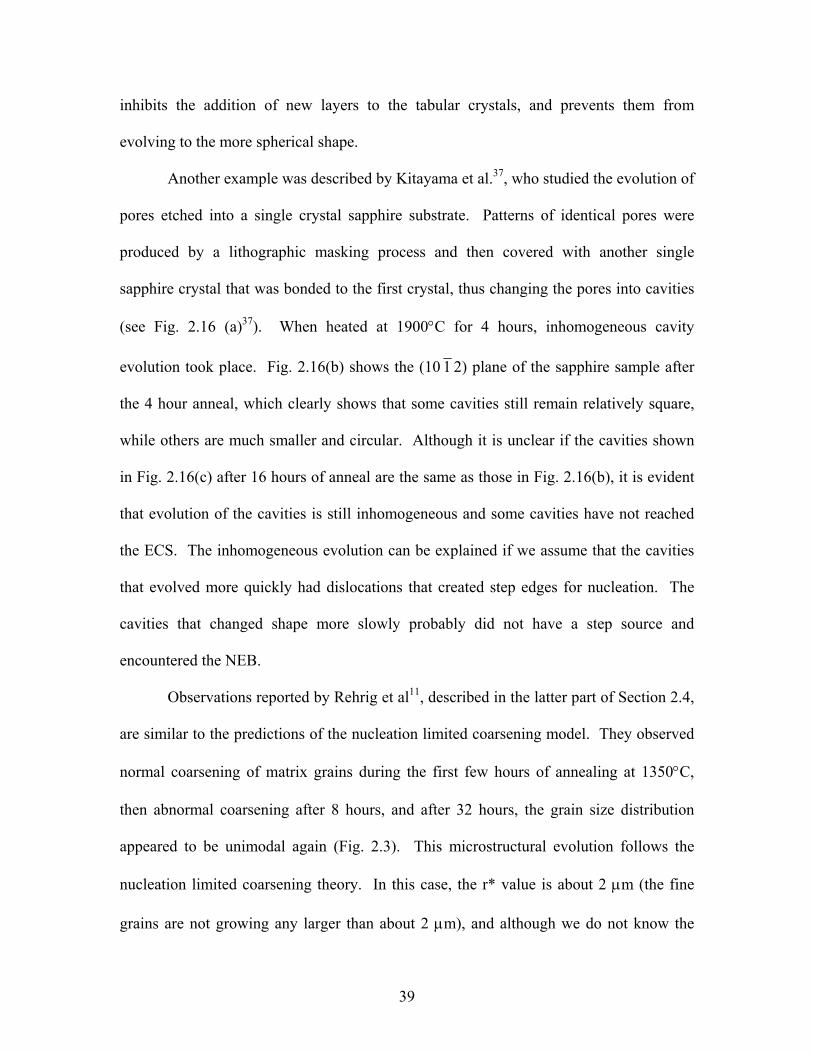
Another example was described by Kitayama et al.37, who studied the evolution of

pores etched into a single crystal sapphire substrate. Patterns of identical pores were

produced by a lithographic masking process and then covered with another single

sapphire crystal that was bonded to the first crystal, thus changing the pores into cavities

(see Fig. 2.16 (a)37). When heated at 1900°C for 4 hours, inhomogeneous cavity

evolution took place. Fig. 2.16(b) shows the (10 1 2) plane of the sapphire sample after

the 4 hour anneal, which clearly shows that some cavities still remain relatively square,

while others are much smaller and circular. Although it is unclear if the cavities shown

in Fig. 2.16(c) after 16 hours of anneal are the same as those in Fig. 2.16(b), it is evident

that evolution of the cavities is still inhomogeneous and some cavities have not reached

the ECS. The inhomogeneous evolution can be explained if we assume that the cavities

that evolved more quickly had dislocations that created step edges for nucleation. The

cavities that changed shape more slowly probably did not have a step source and

encountered the NEB.

Observations reported by Rehrig et al11, described in the latter part of Section 2.4,

are similar to the predictions of the nucleation limited coarsening model. They observed

normal coarsening of matrix grains during the first few hours of annealing at 1350°C,

then abnormal coarsening after 8 hours, and after 32 hours, the grain size distribution

appeared to be unimodal again (Fig. 2.3). This microstructural evolution follows the

nucleation limited coarsening theory. In this case, the r* value is about 2 µm (the fine

grains are not growing any larger than about 2 µm), and although we do not know the

39

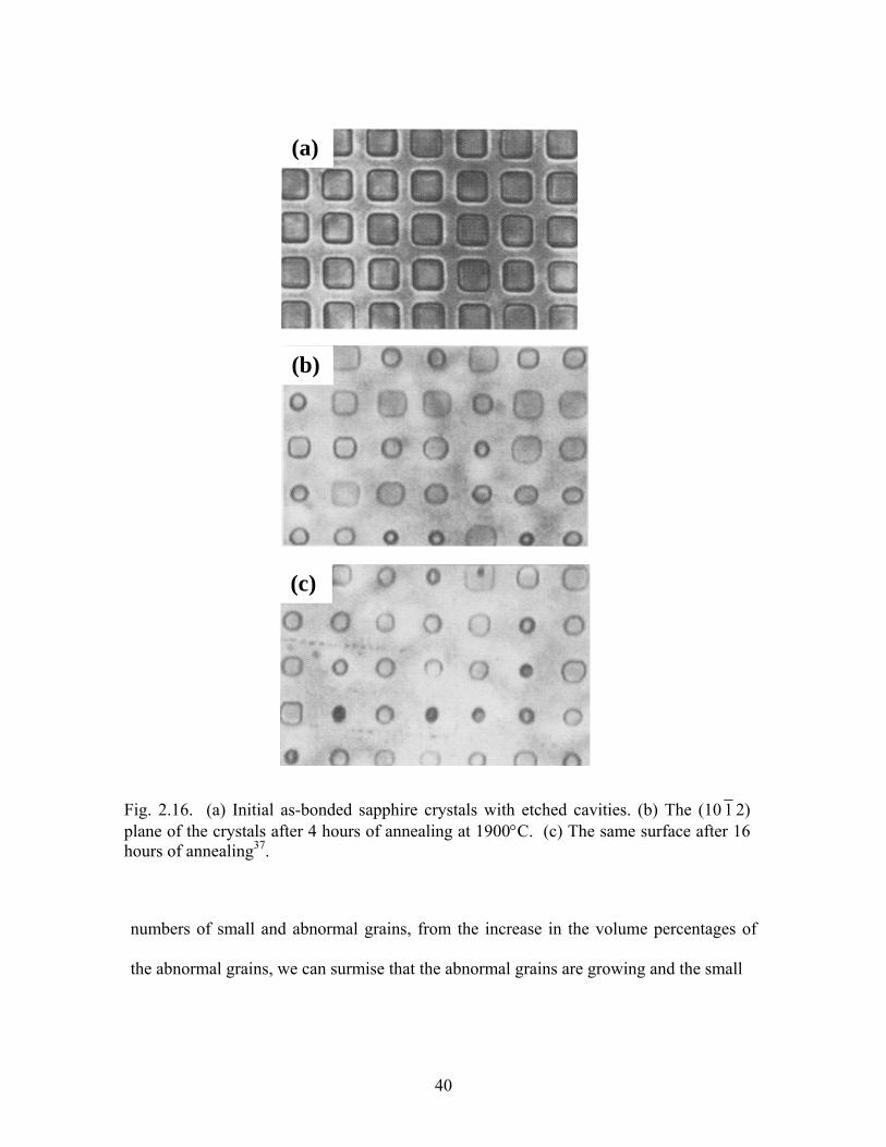
Fig. 2.16. (a) Initial as-bonded sapphire crystals with etched cavities. (b) The (10 1 2) plane of the crystals after 4 hours of annealing at 1900°C. (c) The same surface after 16 hours of annealing37.

(a)

(b)

(c)

numbers of small and abnormal grains, from the increase in the volume percentages of

the abnormal grains, we can surmise that the abnormal grains are growing and the small

40

grains are dissolving. One of the goals of this work is to make observations that will

allow a more direct and unambiguous comparison of the theory for nucleation limited

coarsening.

2.7 System of Interest

The nucleation limited coarsening theory has four predictions. They are: 1) grains

with defects will coarsen at the expense of the small perfect grains, which results in a

transient bimodal grain size distribution, 2) during the bimodal distribution regime, the

number of abnormal grains stays constant, 3) the small perfect grains do not coarsen, and

4) after the perfect grains are consumed, a unimodal grain size distribution develops.

These predictions will be experimentally tested. However the experimental system

cannot mimic the theoretical system. The experimental system will consist of both

coarsening and grain growth. Lu and German38 considered the overall growth of grains

to be comprised of solid-liquid, solid-vapor, and solid-solid growth factors in liquid phase

sintering systems. They proposed that the overall grain growth rate is a sum of the rates

due to those components, weighted by the contiguities of the different phases. In the

same line of reasoning as Lu and German, the belief is that if the effects from grain

growth are accounting for, the nucleation limited coarsening theory can still be tested.

Measurements of the growth rates of faceted particles and the time evolution of

the grain size distribution will be used to characterize the growth mechanisms and

determine the influence of the NEB on coarsening. As described earlier, the signature of

nucleation limited coarsening will be a non-steady state bimodal grain size distribution

and a constant number density of abnormal grains. To make the observations needed to

41

test this model, SrTiO3 crystals will be coarsened in a TiO2 excess liquid phase. The

microstructure will be examined with varying time at a temperature above the eutectic.

The grain sizes will be measured by the linear intercept method from images obtained by

atomic force microscopy and scanning electron microscopy. From the measured grain

sizes, grain size distribution characterizations, the growth rate of the grains, as well as

determinations of number densities of abnormal and small grains can be accomplished.

These results will be compared with those of single-phase SrTiO3 grain growth samples,

prepared and annealed in the same method. By characterizing the single-phase SrTiO3

system, the aim is to deduce the grain growth effects in the two-phase system.

In addition to the grain sizes, the shapes of the coarsening crystals will be

determined. The shapes of the crystals reflect the anisotropy of the interface energy and

are expected to be faceted in some orientations. The orientations of these faceted

interface planes will also be determined.

SrTiO3 was selected primarily because it is a prototypical example of a wide

variety of cubic perovskite materials. The surface properties are of interest for its

potential applications as a substrate for heteroepitaxial films and as a new gate dielectric

for field effect transistors39, 40. In addition, SrTiO3 compacts can be prepared with a

random orientation distribution. A random distribution of crystal orientations is

necessary for unbiased crystal shape analysis.

2.8 References

1. P. Feltham, “Grain Growth in Metals,” Acta Met., 5 [2] 97-105 (1957).

42

2. F. C. Hull, “Plane section and spatial characteristics of equiaxed β-brass grains,”

Mater. Sci. Technol., 4 [9] 778-785 (1988).

3. W. D. Callister, Materials Science and Engineering An Introduction: pp. 177-178.

John Wiley & Sons, Inc., New York, 2000.

4. I. M. Lifshitz, and V. V. Slyozov, “The Kinetics of Precipitation From

Supersaturated Solid Solutions,” J. Phys. Chem. Solids, 19 [1/2] 33-40 (1961).

5. C. Wagner, “Theorie der Alterung von Niederschlägen durch Umlösen (Ostwald-

Reifung),” Z. Elektrochemie, 65 [7/8] 581-591 (1961).

6. W. D. Kingery, H. K. Bowen, and D. R. Uhlmann, Introduction to Ceramics; pp.

461-468. John Wiley & Sons, Inc., New York, 1976.

7. G. W. Greenwood, “The Growth of Dispersed Precipitates in Solutions,” Acta

Metall., 4 [5] 243-248 (1956).

8. T. Li, A. M. Scotch, H. M. Chan, M. P. Harmer, S-E. Park, T. R. Shrout, and J. R.

Michael, “Single Crystals of Pb(Mg1/3Nb2/3)O3-35mol% PbTiO3 from

Polycrystalline Precursors,” J. Am. Ceram. Soc., 81 [1] 244-248 (1998).

9. A. Khan, F. A. Meschke, A. M. Scotch, H. M. Chan, and M. P. Harmer, “Growth

of Pb(Mg1/3Nb2/3)O3-35mol% PbTiO3 Single Crystals from (111) Substrates by

Seeded Polycrystal Conversion,” J. Am. Ceram. Soc., 82 [11] 2958-2962 (1999).

10. M. P. Harmer, H. M. Chan, H-Y. Lee, A. M. Scotch, T. Li, F. Meschke, A. Khan,

“Method for Growing Single Crystals from Polycrystalline Precursors,” U.S.

Patent 6048394 (2000).

43

11. P. W. Rehrig, G. L. Messing, and S. Trolier-McKinstry, “Templated Grain

Growth of Barium Titanate Single Crystals,” J. Am. Ceram. Soc., 83[11] 2654-

2660 (2000).

12. M. M. Seabaugh, I. H. Kerscht, and G. L. Messing, “Texture Development by

Templated Grain Growth I Liquid-Phase-Sintered α-Alumina,” J. Am. Ceram.

Soc., 80 [5] 1181-1188 (1997).

13. C. Zener, “Theory of Spherical Precipitates from Solid Solution,” J.Appl.

Phys.20 950-953 (1949).

14. A. J. Ardell, The Effect of Volume Fraction on Particle Coarsening: Theoretical

Considerations,” Acta Metall., 20 [1] 61-71 (1972).

15. A. D. Brailsford and P. Wynblatt, “The Dependence of Ostwald Ripening

Kinetics on Particle Volume Fraction,” Acta Metall., 27 [3] 489-497 (1979).

16. C. K. L. Davies, P. Nash, and R. N. Stevens, “The Effect of Volume Fraction of

Precipitate on Ostwald Ripening,” Acta Metall., 28 [2] 179-189 (1980).

17. K. Tsumuraya and Y. Miyata, “Coarsening Models Incorporating Both Diffusion

Geometry and Volume Fraction of Particles.” Acta Metall., 31 [3] 437-452

(1983).

18. P. W. Voorhees and M. E. Glicksman, “Solution to the Multi-Particle Diffusion

Problem with Applications to Ostwald Ripening. I. Theory,” Acta Metall., 32 [11]

2001-2011 (1984).

19. P. W. Voorhees and R. J. Schaefer, “IN SITU Observation of Particle Motion and

Diffusion Interactions During Coarsening,” Acta Metall., 35 [2] 327-339 (1987).

44

20. G. J. Shiflet, H. I. Aaronson, and T. H. Courtney, “Kinetics of Coarsening by the

Ledge Mechanism,” Acta Metall., 27 [3] 377-385 (1979).

21. L. Ratke, D. Uffelmann, W. Bender, and P. W. Voorhees, “Theory of Ostwald

Ripening Due to a Second-Order Reaction, “ Scripta Met. et Mater., 33 [3] 363-7

(1995).

22. G. S. Rohrer, C. L. Rohrer, and W. W. Mullins, “Coarsening of Faceted Crystals,”

J. Am. Ceram. Soc. 85 [3] 675-682 (2002).

23. G. Wulff, “Zur Frage der Heschwindigkeit des Wachstums un der Auflosung der

Krystallflachen,” Z. Krist. 34, 449-530 (1901).

24. C. Herring, “Some Theorems on the Free Energy of Crystal Surfaces,” Phys. Rev.

82 [1] 87-93. (1951).

25. D. S. Fisher and J. D. Weeks, “Shape of Crystals at Low Temperatures: Absence

of Quantum Roughening,” Phys. Rev. Lett., 50 [14] 1077-1080 (1983).

26. D. A. Porter and K. E. Easterling, Phase Transformations in Metals and Alloys;

pp. 169. Chapman & Hall, New York, NY, 1995.

27. W. K. Burton and N. Cabrera, “Crystal Growth and Surface Structure,” Discuss.

Faraday Soc., 5, 33-48 (1949).

28. F. C. Frank, “The Influence of Dislocations on Crystal Growth,” Discuss.

Faraday Soc., 5, 48-54 (1949).

29. W. K. Burton, N. Cabrera, and F. C. Frank, “The Growth of Crystals and the

Equilibrium Structure of Their Surfaces,” Philos. Trans. R. Soc. London, Ser. A,

243, 300-358 (1951).

45

30. S. D. Peteves and R. Abbaschian, “Gowth Kinetics of Solid-Liquid Ga Interfaces:

Part I. Experimental,” Metall. Trans. A, 22A [6] 1259-1270 (1991).

31. K. W. Keller, “Modes of Crystal Growth Revealed by Electron Microscopy on

NaCl,” J. Crystal Growth 74 [1] 161-171 (1986).

32. W. C. Carter, A. R. Roosen, J. W. Cahn, and J. E. Taylor, “Shape Evolution by

Surface Diffusion and Surface Attachment Limited Kinetics on Completely

Faceted Surfaces.” Acta Metall. Mater. 43 [12] 4309-23 (1995).

33. W. W. Mullins and G. S. Rohrer, “Nucleation Energy for Volume-Conserving

Shape Changes of faceted Crystals,” J. Am. Ceram. Soc. 83 [1] 214-16 (2000).

34. G. S. Rohrer, C. L. Rohrer, and W. W. Mullins, “Nucleation Energy Barriers for

Volume Conserving Shape Changes of Crystals with Nonequilibrium

Morphologies,” J. Am. Ceram. Soc. 84 [9] 2099-2104 (2001).

35. P. Wynblatt and N. A. Gjostein, “Particle Growth in Model Supported Metal

Catalysts-I. Theory,” Acta Metall., 24 [12] 1165-74 (1976).

36. J. J. Metois and J. C. Heyraud, “Mechanisms of Morphological Change During

the Establishment of the Equilibrium Shape; Lead on Graphite,” J. Crystal

Growth 57 [3] 487-492 (1982).

37. M. Kitayama, T. Narushima, and A. M. Glaeser, “The Wulff Shape of Alumina:

II, Experimental Measurements of Pore Shape Evolution Rates,” J. Am. Ceram.

Soc., 83 [10] 2572-83 (2000).

38. P. Lu and R. M. German, “Multiple Grain Growth Events in Liquid Phase

Sintering,” J. Mater. Sci., 36 [14] 3385-3394 (2001).

46

39. M. Kawasaki, K. Takahashi, T. Maeda, R. Tsuchiya, M. Shinohara, O. Ishiyama,

T. Yonezawa, M. Yoshimoto, and H. Koinuma, "Atomic Control of the SrTiO3

Crystal Surface," Science, 266 [5190], 1540-2 (1994).

40. R. A. McKee, F.J. Walker, M.F. Chisholm, "Crystalline Oxides on Silicon: The

First Five Monolayers," Phys. Rev. Lett. 81 [14] 3014-7 (1998).

47

3. Microstructure Characterization Methods

3.1 Sample Preparation

The following sections describe the methods used to prepare the samples for the

solid-vapor surface energy and grain growth study, the samples for the solid-liquid

coarsening study, and the templated single crystal samples. In addition, descriptions of

microscopy equipment used and analytical techniques will be covered.

3.1.1 Solid-Vapor Study Sample

The samples were fabricated from 99% pure SrTiO3 powder with particle sizes

being < 5 µm from Aldrich Chemical Company, Inc., Milwaukee, WI. A charge of 1.94

±0.01 grams of powder and 2 drops of a polyethylene glycol and dionized water solution

were mixed in a mortar with a pestle. The mixture of powder and binder was uniaxially

pressed to about 1.2×107 pascal or 1700 psi of pressure.

The sample was heated in vacuum (1×104 pascal) at 800°C for 25 hours and then

sintered with reconditioned airflow at 1350°C for 10 hours (ramp rate was 3°C/min). The

grains were grown at 1650°C for 20 hours (same ramp rate) and lapped flat using a

Logitech PM5 automatic polisher (Logitech Ltd. Glasgow, Scotland). The sample was

lapped flat with 3 µm alumina slurry and polished with 0.02 µm colloidal silica slurry for

a ±0.2 µm uniformity throughout the sample. The grains were then grooved at 1400°C for

6 minutes. (10°C/min ramp to/from 1100°C, 30°C/min ramp from/to 1100°C to/from

48

1400°C) Optical microscope images of the entire sample surface were recorded,

including all visible island grains.

After removing 4.65 µm ±0.3 µm by polishing with colloidal silica, the sample

was thermally grooved using the same time and temperature as before. Optical images of

the same ten included grains from the first layer were recorded and the grain boundary

inclination angles were determined by overlapping the first and second layer images.

Grain boundaries, pores, and other surface features were used to align the images of the

two layers. The measurement error is believed to be about 1 pixel, or 0.25 µm. The

boundaries of the included grains were then imaged by atomic force microscopy (AFM),

and the surface orientations mapped by orientation imaging microscopy (OIM).

3.1.2 Solid-Liquid Study Samples

The samples for the SrTiO3 particles in a liquid matrix were prepared in the same

manner as the solid-vapor samples, except the powder included excess ultra high purity

rutile so as to make the composition 20 mole% TiO2, 80 mole% SrTiO31. Therefore, at

the annealing temperature, the sample was comprised of 15 volume% liquid and 85

volume% solid SrTiO3, with the liquid composition being 33.3 mole % SrTiO3 and 66.7

mole % TiO2 (see Fig. 3.1). The powders were mixed with a mortar and pestle, ball

milled with 1 cm diameter glass balls in ethanol for 5 hours at 50 rpm, then dried at 60˚C

for 24 hours. Inspection of the powders at this point by SEM showed agglomerates of

roughly spherical submicron particles with no obvious flat surfaces (Fig. 3.2). The

powder was pressed into pellets as done previously with pure SrTiO3.

49

Fig. 3.1. Phase diagram of SrO-TiO2 system. The red dot indicates the composition of the samples that were annealed at 1500°C1.

1500

The samples were heated in vacuum (1×104 pascal) at 800°C for 25 hours and

allowed to cool at a rate of 2°C/min. Each sample was individually annealed in a box

furnace at 5°C/min ramp to and from 1500°C. Each sample was held at 1500°C for

varying times between 0 and 50 hours. The samples were then lapped with 3 µm alumina

slurry and polished with 0.02 µm colloidal silica slurry for ±0.3 µm uniformity

throughout the sample.

X-ray diffraction was conducted on the 24 h and 50 h samples to determine the

phases. It was determined that for both 24 h and 50 h samples, SrTiO3 and TiO2 (rutile)

50

Fig. 3.2. SEM image of pre-annealed 20 mole% TiO2 – 80 mole% SrTiO3 powder agglomerates.

Fig. 3.3. X-ray diffraction peaks from the 50 h sample.

3020 40 50 60 2*Theta

50 h

Blue = TiO2 RutileRed = SrTiO3

0

500

1000

1500

2000

Counts/sec

3020 40 50 60 2*Theta3020 40 50 60 2*Theta

50 h

Blue = TiO2 Rutile

0

500

1000

1500

2000

Counts/sec

Red = SrTiO3

51

were present as shown in Fig. 3.3. Other phase study conducted was to detect the

presence of the eutectic precipitates. Due to the composition, the eutectic precipitates

Fig. 3.4. (a) A backscattered electron image of the 10 h sample. Arrows point to the eutectic precipitate. (b) A typical eutectic precipitate.

Eutectic Precipitates

52

were few in number and dispersed throughout the sample. A backscattered electron

image indicating the location of a eutectic precipitate is shown in Fig. 3.4(a) and the

precipitate is shown in Fig. 3.4(b).

Each sample was imaged by AFM and the orientations mapped by OIM. OIM

scans were conducted for all samples at a 60° tilt with 20.0 kV beam at a working

distance of 17 mm. All the scans were conducted in a square grid. In other words, the

array of points making up the scan was aligned in a square pattern. The step size, which

sets the distance between each point, was selected based on the grain size for each

sample. For the 0 h sample, the step size was 0.3 µm, for the 5 h sample, the step size

was 0.6 µm, 10 h sample was 1.55 µm, and the 15 h and 24 h samples were both 1.6 µm.

The single-phase solid polycrystalline samples for the grain growth study were

prepared by the same method as the solid-liquid samples, with the only difference being

the powder was 100% SrTiO3 with no TiO2 additions.

3.1.3 Templated Single Crystal Samples

The matrix powder surrounding the template single SrTiO3 crystals was the same

composition as those of the solid-liquid samples. After ball milling the SrTiO3 and rutile

powders, a square piece of SrTiO3 (100) or (111) single crystal was placed in a mold of

powder so that when the powder and single crystal were uniaxially pressed, the single

crystal was located inside the powder compact. The compact was then isostatically

pressed to 2.4×108 pascal (3.5×104 psi) and annealed in a box furnace at 1500°C for 5

hours with ramp rates of 5°C/min.

53

3.2 Optical Microscopy

The Carl Zeiss optical microscope used for this research was paired with the

AnalySIS 3.0 software by Soft Imaging System GmbH for image capture. With the three

objectives on the microscope, the magnification range was adequate to take micrographs

of the grains with a sufficient level of detail. In the solid-vapor study, the optical

microscope was used to obtain images of grain boundary locations of included grains.

An example is shown in Fig. 3.5.

3.3 Atomic Force Microscopy

A Cp AFM by TM Microscopes (originally Park Scientific Instruments,

Sunnyvale, CA) controlled by the PSI ProScan1.5 software was used in this research.

Gold-coated Si3N4 cantilever tips were used to image the surfaces of the samples in

contact mode. The scan sizes and height (gray scale) contrast were selected to be

compatible with the features of interest. All scans were conducted with the 100 µm

scanner.

The scanner houses a piezoelectric tube, to which the sample holder is connected2.

The tube bends back and forth when voltages are applied. This motion moves the sample

under the probe tip in a raster pattern. In contact mode, while the sample is being

scanned, the cantilever bends from the repulsive forces between the atoms in the probe

tip and the atoms on the surface of the sample. A sensor detects the deflection and moves

the sample on the scanner up or down in the z direction to keep the displacement

constant. This z motion corresponds to the surface topography and becomes a scanned

image of the type illustrated in Fig. 3.6.

54

20 µm

Fig. 3.5. Optical image of an included SrTiO3 grain.

(a) (b)

Fig. 3.6. Atomic Force Microscopy image of (a) the same included grain as in Fig. 3.3, and (b) a three-dimensional rendering of a section of the thermally grooved grain boundary.

20 µm

5 µm

1 µm

5 µm

0.6 µm

0

55

3.4 Orientation Imaging Microscopy

The orientation image microscope (TexSEM Laboratories, Inc. of Provo, UT.)

was used to obtain electron backscattered diffraction (EBSD) patterns of crystals. This

orientation imaging microscope (OIM) was connected to a XL40 FEG (Phillips,

Eindhoven, The Netherlands) scanning electron microscope (SEM). The samples were

attached to flat SEM stubs using carbon adhesives, and coated with thin layers of carbon

to prevent charging. The carbon was applied to the samples under 133 pascal (1 Torr) of

vacuum by the SPI Supplies carbon coater module, installed with a carbon fiber head.

All OIM imaging was conducted at a 60° stage tilt, with 20.0 kV accelerating voltage and

a spot size of 5.

The schematic of the OIM system is shown in Fig. 3.7 and the operation of the

Fig. 3.7. A schematic of the orientation imaging microscope.

Electro nBeam

Stage Control

Unit

Sample

Phosphor screen

CCD Camera

SEM Control

Unit

CameraControl

Unit

COMPUTER

Move Beam/Stage

Process Image

Record Data

Index EBSP

56

microscope will be briefly described here3, 4. The incident electron beam penetrates the

surface of the tilted sample and emits backscattered electrons that have diffracted in the

surface region. These electrons excite a phosphor screen and produce photons. The

photons are detected by the charge coupled device (CCD) camera, which digitizes the

Kikuchi patterns. An example of a pattern is shown in Fig. 3.8.

The pattern undergoes an image processing algorithm, called a Hough transform,

and the location of the bands are plotted as points in the (ρ,θ) coordinates of the Hough

space. The position of triplets, or groups of three bands, is matched with sample

symmetry and diffraction pattern center information to determine the best index solution

for the intersection points of the bands.

Fig. 3.8. An EBSP (Kikuchi pattern) of a SrTiO3 crystal.

57

For each indexed pattern of a point on a crystal, there are associated Bunge Euler

angles, notated as, φ1, Φ, φ2, which specify the transformation that aligns the reference

direction on the microscope stage to the local orientation of the crystal lattice vectors. To

align the crystal and stage reference axes, the sample frame is rotated through an angle of

φ1 about the Zs axis, then an angle of Φ about the Xs axis, and lastly through an angle of

(a)

sample

crystal

Fig. 3.9. Schematic representation of the transformation from the sample coordinate to the crystal coordinate system if the crystal was oriented with respect to the sample as in (a). (b) Transformation from the sample coordinate system xs to an intermediate coordinate system, (c) transformation from the sample zs to the crystal coordinate system, zc, (d) transformation from xs to the crystal coordinate system, xc and ys to yc.

sz

cy

cz

Φ

sy

sxcx

φ2

sc zz =

sxcx

sycy

sx

sz

sy

cx

cyφ1

cz

(d) (b)) (c)

58

Fig. 3.10. An inverse pole figure map of a 15 volume% liquid - 85 volume% solid SrTiO3 sample annealed at 1500°C for 10 h. The standard stereographic triangle on the right indicates the orientations corresponding to the different colors.

φ2 about the Zs axis (see Fig. 3.9). When the crystals’ orientations are plotted in an

inverse pole figure map, the orientations are depicted in different colors. An example of

an inverse pole figure map is shown in Fig. 3.10. This method was used to obtain crystal

orientation data for all the samples examined in this work.

3.5 Scanning Electron Microscopy

The XL30 FEG (Phillips, Eindhoven, The Netherlands) scanning electron

microscope (SEM) was used to obtain images of the samples to determine the grain size

distributions. To prevent charging, the samples were coated with carbon as described in

Section 3.4. All SEM imaging was conducted at a 0° stage tilt, with 20.0 kV accelerating

59

voltage and a spot size of 3. Various magnifications were used to best image the

microstructures. For the 3, 5, and 10 h solid-liquid samples, two magnifications were

used to image the abnormal grains and the much smaller grains. For each low

magnification scan area, high magnifications scans of the same area were acquired. The

linear intercept method was used to calculate the grain size distributions. A cut-off grain

size was determined to obtain grain size data from either the low magnification image or

the high magnification image for the samples with bimodal grain size distributions.

3.6 Analysis

With data collected from the microscopy equipment discussed above, the

following analysis will be conducted. Section 3.6.1 will describe the analysis of the

solid-vapor study to obtain the surface energy anisotropy, and Section 3.6.2 will describe

the solid-liquid coarsening analysis to determine the interface habit planes.

3.6.1 Measurement of Surface Energy Anisotropy

The surface energy anisotropy of SrTiO3 was measured using the thermal groove

technique5. A schematic cross-section of a thermal groove is shown in Fig. 3.11. In this

method, AFM is used to determine the geometry of the thermal grooves of the included

grains and the crystallographic orientations are obtained by OIM. Included grains are

used, since the misorientation is constant around the grain. It is assumed that the grain

boundary energy, γgb, is constant for each included grain. The geometry and orientation

data are correlated to Herring’s6 force balance relation,

0ˆˆ =∂∂

+∑i

iii ii nt

βγ

γ , (3.1)

60

where γi is the excess free energy per unit area of the ith interface, ti is the unit vector that

lies in that interface and is perpendicular to the line of intersection, l, of the three

interfaces, ni is the unit vector normal to the line of intersection (ni = l × ti) and βi is the

right-handed angle of rotation about l. This is depicted in Fig. 3.12.

Measurements of the slope at the groove root directly from AFM profiles have

unavoidable errors that result from the finite shape of the tip. A previous analysis of the

problem illustrated that these errors can be largely avoided by assuming that the groove

has a known quasistatic profile, and then finding the slope at the groove root based on

measurements of the depth and width of sufficiently large grooves7. This indirect

determination at the slope of the root is valid only when the groove is formed by surface

diffusion. There is an inherent approximation in this procedure, since the quasistatic

profile was determined under the assumption that the surface energy is isotropic. The

Fig. 3.11. A schematic of a thermal groove. Ψ is the dihedral angle.

Surface

Crystal 2

Ψs

χ2χ1H

Crystal 1

W

61

errors associated with this approximation have not been quantified. However, since the

majority of the observed grooves have profiles that approximate the expected quasistatic

shape, and past results obtained by this method have been consistent with independent

observations. The largest error is instead thought to arise from the EBSD orientation

measurement (± 5°) and from the assumption that the grain boundary energy is

independent of its orientation3. Each side of the groove is measured independently for

the depth and half width.

Fig. 3.12. Schematics of a thermally grooved triple junction.

22tsγ1n11tsγ G

rainundary

n

bo Crystal 2Crystal 1

2ˆ3n

3tgbγ

l

α

β

interface3

interface 2interface 1

t2

t3^

t1^

lβ

n3 ^ n2 ^

n1^

If the thermal grooves are formed by surface diffusion, the surface energies can be

determined by only measuring the widths and heights of the grooves. Rather than using

the AFM to determine the groove profile, if the grooves are formed by surface diffusion,

a more accurate geometry can be determined by using Robertson’s8 relation of width and

height to the groove profile. If the slope of the plot of the natural log of groove width

versus natural log of time is roughly 1/4, as predicted by Mullins9, then it can be assumed

62

that the grooves formed by surface diffusion and his equation can be used to calculate the

surface diffusion coefficient,

NtvkTWD

SVs 24

4

6.4 γ= , (3.2)

where k is the Boltzmann’s constant, T is the absolute temperature, γSV is the surface

energy, v is the molecular volume, N is the number of diffusing species and t is time.

Another necessary parameter is the orientation of both sides of the thermal

groove. The crystal orientations are determined from EBSP analysis and are expressed in

Euler angles. To transform vectors in the sample reference frame (n) to the crystal

reference frame (z), the following 3×3 matrix is used:

⎢⎢⎢

⎣

⎡

⎥⎥⎥

⎦

⎤

ΦΦ−ΦΦΦ+−Φ−−ΦΦ+Φ−

=Φcscss

sccccssccsscsscsccscsscc

g

11

221212121

221212121

21 ),,(φφ

φφφφφφφφφφφφφφφφφφ

φφ , (3.3)

where c stands for cosine and s for sine. With respect to the variables defined in Figs.

3.11 and 3.13, the surface normal in the sample reference frame is,

ii

i

ii

ii

n

nn

χ

τχτχ

sin)1(

sincoscoscos

3,

2,

1,

−=

=

=

(3.4)

and χ is the partial dihedral angle of the groove on side i, and τ is the in-plane angle.

This vector is transformed to the crystal reference frame by the following relation,

jiji ngz = , (3.5)

where nj is the matrix from Eq. (3.4)

63

The angle of the grain boundary, α, is determined by overlapping the optical

images of the included grains from the first layer and the second layer observed after

serial sectioning several microns, ∆H (see Fig. 3.14). The ∆x values are the distances

between the grain boundaries of the included grains between layer one and layer two.

The angle α is determined by,

⎟⎠⎞

⎜⎝⎛

∆∆

=Hxtanα . (3.6)

The capillarity reconstruction method10 was used to determine surface energy.

This method discretizes the surface normal domains into 15 units of ∆cosθ and ∆φ, which

divides the orientation space into 152 cells of equal area. To apply this method, the

Herring relation is rewritten in terms of the Cahn-Hoffman11, 12 capillarity vector, , iξv

)( 0ˆ321 =×++ lξξξvvv

, (3.7)

Fig. 313. Schematic of an included grain with groove trace segment v perpendicular to the grain boundary, line l perpendicular to v, and the angle τ between the coordinate e1 and v.

1e

2e

Crystal 2 l

v1e

τ

Crystal 1

64

In Eq. (3.7), ξ1, ξ2, and ξ3 are the capillarity vectors associated with the two free surfaces

and the grain boundary, respectively, and l is the unit vector pointing along the line where

the three interfaces meet. For every observed groove root, there is a separate equilibrium

equation with the form of Eq. (3.7) for which we have measured the direction of l and the

directions of the two perpendicular components of each ξ vector. The only unknowns are

the magnitudes of the vectors. It is important that the number of unknown parameters is

smaller than the number of observations. Therefore, the domain of distinguishable

surface normals is discretized and the number of distinct grain boundaries is limited by

making many measurements at a small set of circumferential thermal grooves. To further

simplify the problem, we make the approximation that the energy of each grain boundary

is independent of the interface plane. The errors arising from this approximation are

expected to change signs around the groove circumference and, therefore, partially cancel

Fig. 3.14. (a) Optical images of an included grain the first and second layer, and (b) a schematic of the included grains.

∆H

(b) (a) ∆x

∆H α

65

as data from a large number of grooves is averaged. Using this approximation, each

circumferential groove adds only a single unknown parameter to the set of equilibrium

equations. Therefore, after a sufficient number of observations, an iterative procedure,

originally described by Morawiec13, can be used to find the set of capillarity vectors that

most nearly satisfies this system of linear equations.

A Fourier function was used smooth out the discrete surface energy points. The

Fourier series function is,

[ ] [ ]∑∑

= = ⎪⎭

⎪⎬⎫

⎪⎩

⎪⎨⎧

+

−++−

+=

R

i

R

j ij

ijijij

s

jid

jicjibjia

1 0

)100(

)sin()2sin(

)sin(1)2cos()cos()2sin()cos(1)2cos(

),(

ϕθ

ϕθϕθϕθ

γϕθγ

(3.8)

where θ and ϕ are angles in the spherical coordinates and R is the series order. The

program written in Fortran, which determines the coefficients of the series from inputs of

γ, θ, and ϕ values, is in the Appendix A14. Although small fluctuations in the data are

smoothed, determining the surface energy by a Fourier series can add artificial peaks and

dips that result from the shapes of the trigonometric functions and the finite order of the

series.

The equilibrium shape can be determined by the Wulff construction. Using the

surface energy results from the capillarity reconstruction method, a point on the surface

of the Wulff shape can be found for each orientation present on the Wulff shape. The

spaces between the points can be filled in by the use of the software Qhull and the

approximate equilibrium shape is constructed with GEOMVIEW.

66

3.6.2 Coarsening Analysis

For the coarsening study, the sizes and shapes of the grains are of interest. The

sizes will allow us to compare experimental results of the grain size distribution and

coarsening rate to the predictions of the LSW coarsening theory. We also need to

investigate the shapes of the grains during coarsening to understand how the driving force

for growth is affected by morphological changes. The objective is to determine the

distributions of SrTiO3 crystals surfaces, λ(n), where n is the interface normal in the

crystal reference frame and λ is the relative area, measured in multiples of a random

distribution (MRD). For an isotropic distribution of interfaces, λ is unity for all n. In the

anisotropic case, values of λ above or below unity indicate relative areas larger or smaller

than expected in the isotropic case.

Fig. 3.15. A planar AFM image of grains coarsened at 1500°C for 24 hours. The green line indicates a solid-liquid interface.

10µm

0.1 µm

0

67

A stereological approach was used to determine the solid-liquid interface habit

planes. On a planar section, the interface plane appears as a line, as illustrated in Fig.

3.15. The direction of the line in the laboratory reference frame can be determined from

AFM images and the line can be transformed to the crystal reference frame using the

orientations measured by EBSD. The coordinates of the line segment endpoints were

measured using a program that records the data as they are traced using a computer

mouse. The stereological calculation can begin when this data is combined with the

orientations of that grain.

The analysis, which has been described in two recent papers can be explained

briefly in the following way15, 16. Each observed interface trace, ijl , must be part of a

habit plane that obeys the condition 0ˆ =⋅ ijkij nl as shown in Fig. 3.16(a). In other words,

, the normals of possible habit planes, are in the ijkn ijl zone as depicted in Fig. 3.16(b).

The vectors in the sample reference frame are transformed into the crystal reference

frame vectors, by,

ijkn

'n

mijk

lml ngn ˆ),,(ˆ 21' φφ Φ= , (3.9)

where g(φ1, Φ, φ2) is specified by Eq. (3.3). To account for the fact that a random section

plane is more likely to intersect a perpendicular plane than a parallel one, we multiply the

observed length by a factor of sinθk, where θk is the inclination of the interface plane as

illustrated in Fig. 3.17.

The probability function, which describes the probability that a particular length

of line is of a plane with the normal is, 'n

68

∑∑

=kji kij

kji kijijki

l

lngnp

,,

,,'

sin

sinˆ)ˆ(

θ

θr , (3.10)

where i is the grain number, j the line segment, and k specifies a discrete orientation. The

domain of orientations was parameterized by φ and cosθ into cells of equal area. A

schematic of half of a hemisphere is shown in Fig. 3.18. With 10° resolution, (θ = 10), k

Fig. 3.16. (a) The line segment lij has an infinite number of habit planes with normal nijk. (b) In the crystal reference frame, the normals nijk must lie in the lij zone.

Fig. 3.17. A schematic of the boundary line ijl

r, the interface plane inclination angle θk,

and possible normals of the habit plane which form an arc. ijkn

φ

θk

x

ijkn

ijlr

y

lij

nijk

(b) (a)

nijk

lij

69

is 9, and with 36 segments of φ, the total number of equal area cells is 324. When )ˆ( 'npr

is computed by summing a large number of line segments, the correct habit planes occur

with a probability that is higher than the incorrect habit planes and )ˆ( 'npr is maximized

with these orientations (see Fig. 3.19).

For comparison, solid-liquid interface line segments were also extracted using the

TexSEM OIM Analysis 3 software. Since liquid does not diffract well, the liquid phase

data points were assumed to have confidence indexes of less than 0.l. Euler angle value

of (0, 0, 0) was artificially given to theses data points (using a program presented in

Appendix B). To discard single points within the liquid phase with confidence indices of

greater than 0.1, the minimum pixel size of an acceptable grain was set to 5 pixels.

The software then reconstructed and extracted interface and grain boundary

segments by a method described by Wright and Larsen17. Since only interphase

boundary segments are needed, boundary segments with only one neighboring crystal

Fig. 3.18. Discretized quarter of the orientation space. All cells have equal area.

φ

θ

70

having (0, 0, 0) Euler angles were used for the habit plane analysis. The habit plane

results from this data were consistent with results obtained by hand tracing.

Fig. 3.19. Correct habit plane normals become evident with more interface traces.

4.00

0

0 1.0

0.00

2.0

3.00

3.7 Misorientation Averaged Distribution of SrTiO3 Grain Boundary

Planes

The same orientation averaged stereological calculation can be conducted on a

single phase SrTiO3 sample to determine the grain boundary plane distribution. The

grain boundary distribution, λ(∆g,n), is defined as the relative areas of grain boundaries

with a misorientation, ∆g, and boundary plane normal, n, in units of MRD. The methods

used to measure λ(∆g,n) for SrTiO3 are the same as previously developed for the study of

MgO; a detailed account of these methods has already been published18.

71

3.8 References

1. E. M. Levin, C. R. Robbins, and H. F. McMurdie, Phase diagrams for ceramists

1969 Supplement; M. K. Reser ed., American Ceramic Society, Columbus, OH,

Figure 2334 (1969).

2. User’s Guide to AutoProbe CP: Part I: Learning to Use AutoProbe CP: Basic

Imaging Techniques 48-101-1121, Rev. A. For PSI ProScan Software Version 1.5

pp. 2-21 (1998).

3. V. Randle and O. Engler, Introduction to Texture Analysis Macrotexture,

Microtexture and Orientation Mapping; pp 165-167. Gordon and Breach Science

Publishers, Amsterdam, The Netherlands, 2000.

4. B. El-Dasher, “Understanding the TSL EBSP Data Collection System,” Mini-

course, Pittsburgh, PA, September 19, 2002.

5. D. M. Saylor, D. E. Mason, and G. S. Rohrer, “Experimental Method for

Determining Surface Energy Anisotropy and Its Application to Magnesia,” J. Am.

Ceram. Soc. 83 [5] 1226-32 (2000).

6. C. Herring, "Surface Tension as a Motivation for Sintering"; pp. 143-79 in The

Physics of Powder Metallurgy. Edited by W.E. Kingston. McGraw Hill, New

York, 1951.

7. D. M. Saylor and G. S. Rohrer, “Measuring the Influence of Grain-Boundary

Misorientation on Thermal Groove Geometry in Ceramic Polycrystals,” J. Am.

Ceram. Soc. 82 [6] 1529-36 (1999).

8. W. M. Robertson, “Grain-Boundary Grooving by Surface Diffusion for Finite

Surface Slopes,” J. Appl. Phys. 42 [1] 463-7 (1971).

72

9. W. W. Mullins, “Theory of Thermal Grooving,” J. Appl. Phys. 28 [3] 333-339

(1957).

10. D. M. Saylor and G.S. Rohrer, “Evaluating Anisotropic Surface Energies Using

the Capillarity Vector Reconstruction Method,” Interface Science 9 [1/2], 35-42

(2001).

11. D. W. Hoffman and J. W. Cahn, “A Vector Thermodynamics for Anisotropic

Surfaces. I. Fundamentals and Applications to Plane Surface Junctions,” Surface

Science 31 [1] 368-388 (1972).

12. J. W. Cahn and D. W. Hoffman, “A Vector Thermodynamics for Anisotropic

Surfaces. II. Curved and Faceted Surfaces,” Acta Metall., 22 [10] 1205-1214

(1974).

13. A. Morawiec, "Method to Calculate the Grain Boundary Energy Distribution over

the Space of Macroscopic Boundary Parameters from the Geometry of Triple

Junctions," Acta Mater. 48 [13] 3525-32 (2000).

14. W. H. Press, B. P. Flannery, S. A. Teukolsky, W. T. Vetterling, Numerical

Recipes in Fortran; p.668. Cambridge University Press, Cambridge, MA, 1992

15. D. M. Saylor and G. S. Rohrer, “Determining Crystal Habits from Observations

of Planar Sections,” J. Am. Ceram. Soc., 85 [11] 2799-2804 (2002).

16. C.-S. Kim and G. S. Rohrer, “Geometric and Crystallographic Characterization of

WC surfaces and Grain Boundaries in WC-Co Composites,” Interface Science 12

[1] 19-27 (2004).

17. S. I. Wright and R. J. Larsen, ”Extracting Twins from Orientation Imaging

Microscopy Scan Data,” J. Micro. 205 [3] 245-52 (2002).

73

18. D. M. Saylor, A. Morawiec, and G. S. Rohrer, “Distribution of Grain Boundaries

in Magnesia as a Function of Five Macroscopic Parameters,” Acta Mater., 51 [13]

3663-3674 (2003).

74

4. SrTiO3 Solid-Vapor Surface Energy

4.1 Results

In this section, the results of the solid-vapor study will be discussed. These

results are documented in a recent paper1 but will be covered in detail here. As discussed

in Section 3.6.1, the measurement of the surface energy anisotropy depends on thermal

grooves that are formed by surface diffusion. Mullin’s2 equation for the width as a

function of time (Eq. 3.2) shows that if grooves are formed by surface diffusion, the

width will be proportional to t1/4. The data in Fig. 4.1 show the width of three different

grooves that were measured at the same location after 6 minutes, 12 minutes, and 60

minutes. All three have slopes very close to ¼ and we therefore conclude that these

Fig. 4.1. Three examples of the ln(w) vs. ln(t) relations. The bottom line has a slope of 0.26 with a coefficient of determination value, R2, of 0.998, the middle line has a slope of 0.25 with R2 of 0.999, and the top line has a slope of 0.23 with a R2 of 0.987.

ln(W

) (µm

)

ln(t) (min) 4.5 43.532.52

2

1.4 1.7

0.5 1.5

0.8 1.1

m = 0.25

75

grooves were formed by surface diffusion.

The surface diffusion coefficient of SrTiO3 at 1400°C was calculated by using Eq.

(3.2),

NtvkTWD

SVs 24

4

6.4 γ= , (3.2)

estimating γSV to be 1 J/m2, v as 5.74×10-29 m3/molecule, and N as v-2/3. The diffusion

coefficient ranged from 1x10-10 m2/s to 1x10-9 m2/s. These observations are consistent

with the earlier results by Jin et al.3 who obtained values close to ~0.5 x10-10 m2/s.

As mentioned in Section 3.6.1, the surface energy analysis depends on measuring

thermal grooves formed by surface diffusion around island grains. After determining the

location of the included grains, a 4.65 µm layer was removed by polishing. The included

grains were located in the second layer, and optical and AFM images were recorded. An

optical image of one such included grain is shown in Fig. 3.3. A large AFM image that

encompasses the whole included grain is shown in Fig. 3.4(a).

AFM images of the grain boundaries were recorded (Fig. 3.4(b)) such that each

image overlapped with the previous image. Continuing the scans around the grain

Fig. 4.2. An example of a thermal groove trace perpendicular to the grain boundary.

heig

ht, µ

m

in plane distance, µm

0.8 0.6 0.4

0 0.2

12 108642 0

76

allowed the whole grain boundary to be mapped. By examining the topography data

along lines perpendicular to the grain boundary groove (Fig. 4.2), it was possible to

measure the central minimum and the maxima flanking the groove. From these

measurements, the width and the maximum height of the groove were determined. A

total of 479 groove traces were measured around the periphery of 10 included grains. To

determine the orientation of the surfaces at the groove root, it was necessary to obtain the

orientation of the grain on both sides of the boundary. Orientations were measured using

EBSPs. For a reliable analysis, it is important to sample all distinguishable orientations.

With both the groove geometry and grain orientation data, the surface normals were

calculated. The distribution of observed surface orientations at the groove root is plotted

in a standard stereographic triangle (SST) shown in Fig. 4.3.

The groove boundary inclination angle, α, (Fig. 3.12(b)) was found to range from

–33° to 49° with 68% of the boundaries being between –5° and 0°. Using these data, the

Fig. 4.3. Surface normal observations plotted in the SST.

(111)

(110)(100)

77

relative surface energy as a function of orientation, γ(n), was calculated using the

procedure described in Section 3.5.1, and the results are shown in Fig. 4.4.

Fig. 4.4. Stereographic projection of the surface energies projected on the <100>.

a.u.

Fig. 4.5. The discrete surface energy data plotted in solid diamonds and the Fourier series data points plotted as stars.

0.9

0.93

0.96

0.99

1.02

1.05

1.08

0 15 30 45 60 75 90 105 120 135

θ (degrees)

γ(n)

(arb

.)

dataR=2 fit

(100)

(110)(111)

(100)

78

The relative energy around the perimeter of the standard stereographic triangle is

shown plotted with solid diamonds in Fig. 4.5. The minimum energy is at (100) and the

total anisotropy is 10%. To make an assessment of the uncertainty in the energy model,

we quantify the extent to which it satisfies the equilibrium equations. Each discrete

surface normal is involved in as many as 360 equilibrium equations at all the triple

junctions. While the right hand side of Eq. (3.9) is ideally zero, in reality there will be a

small residual. Assuming that the source of the residual is evenly distributed among the

three interfaces at the junction, we assign one third of the residual to the surface normal

of interest. We can then adjust the energy of the orientation by this amount to create a

hypothetical corrected energy. Since this process can be repeated for each equation a

surface normal is involved in, we can define a distribution of corrected energies with

standard deviation that is determined by the variation in the magnitudes of the residuals.

Thus, the standard deviation of these corrected energies is a measure of how well the

energy model actually satisfies all of the equations. Thus we use this quantity as a

measure of the uncertainty. These standard deviations are plotted in Fig. 4.6 and

illustrate that the typical uncertainty, with respect to satisfying the condition for local

equilibrium, is about 0.03. This plot also shows that the error is sharply peaked at the

(110) orientation. Based on this analysis, we assign the following values for the relative

energies and uncertainties (the units are arbitrary):

.01.002.106.001.103.093.0

111

110

100

±=±=±=

γγγ

79

Fig. 4.6. Residuals of Eq. (3.9) which represent deviations from ideal behavior, plotted for all orientations.

a.u.

Fig. 4.5 also shows that the 111 and the 110 energies are similar. The

fluctuations between 40° and 105° are comparable to the experimental uncertainty and

are not meaningful. However they greatly influence the construction of the equilibrium

crystal shape (ECS). Even the small minima imply the existence of facets on the ECS.

The capillarity vector reconstruction method produces a discrete representation of the

energy. To express the data in a continuous manner and smooth the unrealistic

fluctuations, a linear least squares fit of the Fourier series in Eq. (3.8) was performed. A

comparison of the discrete data and the fitted series are shown in Fig. 4.5. The

coefficients for the fitted series are shown in Table 4.1.

The plot of surface structure as a function of crystallographic orientation on a

standard stereographic triangle (see Fig. 4.7(a)) is referred to as an orientation stability

plot. Note that the open diamond near (111) corresponds to the surface illustrated in Fig.

80

4.7(b) that is bounded by two different facets, and the open diamond near the center of

the SST corresponds to the surface bounded by three facets are illustrated in Fig. 4.7(c).

The faceting to two different orientations occurs when the surface at that orientation

lowers its energy by forming surfaces of two different, more stable orientations. In the

Table 4.1. Coefficients to the Fourier series a10 a11 a20 a21 a220.581 -0.061 -0.106 0.206 -0.191 b10 b11 b20 b21 b220.550 -0.146 -0.129 0.294 -0.353 c11 c21 c22 -1.100 -0.242 0.116 d11 d21 d22 -0.899 -0.333 0.270

(a) (b)

(c)

Fig. 4.7. (a). SST of faceted and non-faceted orientations. (b) The open diamond at the edge, close to (111) is the orientation of a surface bounded by two different facets. (c). The surface bounded by three different facets was observed at the center.

(110)(100)

(111)

400

0

Å

1 µm

1 µm

Å 700

0

Not faceted

Faceted

81

case with Fig. 4.7(b), the two stable surfaces are 111 and a complex orientation

approximately 15° from 100. The orientation bounded by three different facets is also

unstable, but does not lie in a zone with two stable orientations. Fig. 4.7(c) shows a

surface that formed a 111 facet, a complex facet about 5° from 110, and a complex

facet inclined by about 15° from 100. The plot reveals the trends that flat orientations

occur in distinct fields surrounding the 100 and 110 poles and that other orientations

are faceted. While no perfectly flat surfaces were found near the 111 orientation, these

faceted surfaces were made up of large, flat 111 terraces, separated by steps with

heights greater than 2 nm (see Fig. 4.7(b)). This suggests that the 111 surface is part of

the equilibrium crystal shape, but that for surfaces near this orientation, the steps bunch to

form facets with inclined orientations. This is in contrast to orientations close to the

110 and 100 surfaces, where single layer steps tend to be separated so that the

surface remains flat and, a wider range of stable orientations are permitted.

By applying the Wulff construction to γ(n), we can determine an ECS and see if

the missing orientations correlate with the orientation stability plot. In this discussion,

we use the discrete reconstructed γ(n). When we do this, we find that orientations within

15° of 100 and orientations within 5° of 110 are on the ECS; most of the other

orientations are missing. This result is consistent with the orientation stability plot in Fig.

4.7(a). However the ECS also contains features that are inconsistent with this plot. For

example, the Wulff construction leads to the result that several orientations inclined by

about 15 ° from 111 are part of the ECS, while 111 is not. The appearance of these

facets on the ECS is the result of a small downward fluctuation in the reconstructed γ(n)

at these surface normals (note in Fig. 4.5 that γ(n) decreases by a small amount for

82

surfaces inclined from (111)). Since this downward fluctuation is within the

experimental uncertainty, it should not be considered significant. This illustrates two

important points. The first is that small changes in γ(n), within the range of the

experimental uncertainty, can have dramatic effects on the ECS. The second is that the

current experimental techniques do not have the precision to exactly determine the ECS

from observations of thermal grooves.

On the other hand, by combining the reconstructed γ(n) with the orientation

stability data from observations of surface faceting, it is possible to develop an acceptable

model for the ECS. For example, from γ(n) and the orientation stability map, we know

that 100 and 110 surfaces are on the ECS, as are surfaces close to these orientations.

Furthermore, the appearance of 111 terraces on faceted surfaces in the vicinity of this

orientation indicates that it too is part of the ECS. Orientations not on the ECS are

bounded by either two or three facets. While current measurements do not exactly define

the boundaries between the orientations bounded by two or three facets, the surfaces with

three facets are clustered near the center of the standard stereographic triangle; an

example of such a surface is illustrated in Fig. 4.7(c). The three facet planes are 111, a

complex plane about 5° from 110, and a complex plane inclined by about 15° from

100. Orientations on great circles connecting two surfaces that are part of the ECS

break up into two facets. For example, within experimental error, the surface in Fig.

4.7(b) is on the great circle joining (111) and a complex plane near (100). Similar

surfaces are observed along the other lines that connect orientations that are part of the

ECS.

83

Based on this information, the ECS is approximately cube shaped, with the edges

and corners truncated by 110 and 111 planes. Furthermore, while the 111 facets

will be very flat, the presence of surfaces vicinal to 100 and 110 means that the flat

low index facets will be surrounded by curved surfaces meeting each other at sharp

edges. The ECS illustrated in Fig. 4.8 reflects the above considerations and is consistent

with both the reconstructed energy and the orientation stability data. While the identity

of the surfaces that are part of the ECS and the places that they intersect are relatively

certain, other features that depend on the details of the function are less certain. For

example, the shape features six equivalent caps made up of 100 and surfaces inclined

by ≤ 15°. While the size of the cap is relatively certain, the relative areas of each of the

surfaces that make up the cap are uncertain. The cap might be gently curved, with each

surface making up a roughly equal contribution to the total area, or it might be a mostly

flat 100 surface with the curvature concentrated near the edges where it meets 111

and a surface near 110.

Fig. 4.8. Equilibrium crystal shape of SrTiO3 at 1400°C in air.

84

4.2 Discussion

The result that the (100) surface has the minimum energy is consistent with bulk

termination models. While it is difficult to predict the relaxation processes involved in

surface formation, the first order contribution to the surface energy from the bond rupture

process is relatively easy to estimate. When the perovskite structure is cleaved parallel to

(100), one Ti-O and four Sr-O bonds are ruptured. To create the (110) surface, at least

two Ti-O and five Sr-O bonds must be ruptured. To create the (111) surface, at least three

Ti-O and three Sr-O bonds must be ruptured. If we take Pauling's4 electrostatic bond

valences (p) to be measures of the relative bond energies, then the Ti-O bond has a

strength of 2/3 and the Sr-O bond a strength of 1/6. Therefore, the ratios of the total bond

valences lost during the creation of each surface is p110/p100 = 1.62 and p111/p100 = 1.87.

Hence, creating (110) and (111) surfaces requires that a larger number of stronger bonds

be broken than when creating the (100) surface. This conclusion is consistent with the

observation that (110) and (111) have similar energies that are significantly higher than

(100).

Electrostatic considerations also suggest that the (100) surface energy should be

lower than the others. When this surface is created by cleavage, equal areas of TiO2

terminated crystal and SrO terminated crystal must be created. Each of these surfaces is

charge neutral and referred to as nonpolar. Cleavage leaves charged surface termination

layers for other orientations. These are usually referred to as polar surfaces. Since polar

surfaces have permanent dipole moments, they are expected to have relatively higher

energies5. Therefore, it is expected that surfaces away from the nonpolar (100)

orientations have dipolar charge, which can contribute to the increase in the energy.

85

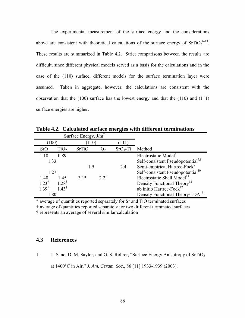
The experimental measurement of the surface energy and the considerations

above are consistent with theoretical calculations of the surface energy of SrTiO36-13.

These results are summarized in Table 4.2. Strict comparisons between the results are

difficult, since different physical models served as a basis for the calculations and in the

case of the (110) surface, different models for the surface termination layer were

assumed. Taken in aggregate, however, the calculations are consistent with the

observation that the (100) surface has the lowest energy and that the (110) and (111)

surface energies are higher.

Table 4.2. Calculated surface energies with different terminations

Surface Energy, J/m2 (100) (110) (111)

SrO TiO2 SrTiO O2 SrO3-Ti Method 1.10 0.89 Electrostatic Model6

1.33 Self-consistent Pseudopotential7,8

1.9 2.4 Semi-empirical Hartree-Fock9

1.27 Self-consistent Pseudopotential10

1.40 1.45 3.1* 2.2+ Electrostatic Shell Model11

1.23† 1.28† Density Functional Theory12

1.39† 1.43† ab initio Hartree-Fock12

1.80 Density Functional Theory/LDA13

* average of quantities reported separately for Sr and TiO terminated surfaces + average of quantities reported separately for two different terminated surfaces † represents an average of several similar calculation

4.3 References

1. T. Sano, D. M. Saylor, and G. S. Rohrer, “Surface Energy Anisotropy of SrTiO3

at 1400°C in Air,” J. Am. Ceram. Soc., 86 [11] 1933-1939 (2003).

86

2. W. W. Mullins, “Theory of Thermal Grooving,” J. Appl. Phys., 28 [3] 333-339

(1957).

3. M. Jin, E. Shimada, and Y. Ikuma, “Grain Boundary Grooving by Surface

Diffusion in SrTiO3 Bicrystal,” J. Mater. Res., 14 [6] 2548-53 (1999).

4. L. Pauling. "The principles determining the structure of complex ionic crystals",

J. Am. Chem. Soc., 51 1010-26 (1929).

5. P.W. Tasker, "The Stability of Ionic Crystal Surfaces," J. Phys. C: Solid State

Phys., 12 [22] 4977-4984 (1979).

6. W. C. Mackrodt, "Atomistic Simulation of Oxide Surfaces," Phys. Chem. Min.,

15 [3] 228-237 (1988).

7. J. Padilla and D. Vanderbilt, "Ab Initio Study of SrTiO3 Surfaces," Surf. Sci., 418

[1] 64-70 (1998).

8. B. Meyer, J. Padilla, and D. Vanderbilt, "Theory of PbTiO3, BaTiO3, and SrTiO3

Surfaces," Faraday Discuss., Surface Science and Metal Oxides 114 395-405

(1999).

9. A. Pojani, F. Finocchi, and C. Noguera, " Polarity on the SrTiO3 (111) and (110)

Surfaces," Surf. Sci., 442 [2] 179-198 (1999).

10. C. Cheng, K. Kunc, and M. H. Lee, "Structural Relaxation and Longitudinal

Dipole Moment of SrTiO3 (001) (1x1) Surfaces," Phys. Rev. B, 62 [15], 10409-

10418 (2000).

11. E. Heifets, E. A. Kotomin, and J. Maier, "Semi-empirical Simulations of Surface

Relaxation for Perovskite Titanates," Surf. Sci., 462 [1-3] 19-35 (2000).

87

12. E. Heifets, R. I. Eglitis, E. A. Kotomin, J. Maier, and G. Borstel, "Ab Initio

Modeling of Surface Structure for SrTiO3 Perovskite Crystals," Phys. Rev. B, 64

[23] 235417-235422 (2001).

13. X. Zhang and A. Demkov, "Steps on the (001) SrTiO3 Surface," J. Vac. Sci.

Technol. B, 20 [4] 1664-1670 (2002).

88

5. Grain Boundary Analysis

5.1 Orientation Distribution

Recently it was observed in MgO1 that the population of grain boundaries was

inversely correlated to the sum of the surface energies of the planes on either side of the

boundary. To determine if this trend also occurs in SrTiO3, the grain boundary character

distribution was determined by the method explained in Section 3.7, and compared to the

measured surface energies described in Chapter 4.

Fig. 5.1 shows the comparison between the surface energy as a function of

orientation and the grain boundary plane distribution. Clearly, at the orientations where

(a) (b)

Fig. 5.1. (a) Misorientation averaged distribution of grain boundary planes. (b) Surface energy projection.

MRD a.u.

88

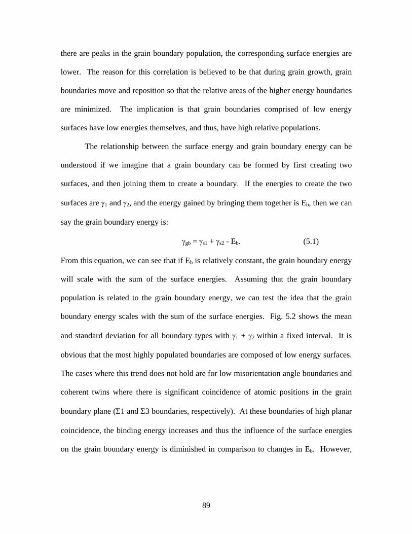
there are peaks in the grain boundary population, the corresponding surface energies are

lower. The reason for this correlation is believed to be that during grain growth, grain

boundaries move and reposition so that the relative areas of the higher energy boundaries

are minimized. The implication is that grain boundaries comprised of low energy

surfaces have low energies themselves, and thus, have high relative populations.

The relationship between the surface energy and grain boundary energy can be

understood if we imagine that a grain boundary can be formed by first creating two

surfaces, and then joining them to create a boundary. If the energies to create the two

surfaces are γ1 and γ2, and the energy gained by bringing them together is Eb, then we can

say the grain boundary energy is:

γgb = γs1 + γs2 - Eb. (5.1)

From this equation, we can see that if Eb is relatively constant, the grain boundary energy

will scale with the sum of the surface energies. Assuming that the grain boundary

population is related to the grain boundary energy, we can test the idea that the grain

boundary energy scales with the sum of the surface energies. Fig. 5.2 shows the mean

and standard deviation for all boundary types with γ1 + γ2 within a fixed interval. It is

obvious that the most highly populated boundaries are composed of low energy surfaces.

The cases where this trend does not hold are for low misorientation angle boundaries and

coherent twins where there is significant coincidence of atomic positions in the grain

boundary plane (Σ1 and Σ3 boundaries, respectively). At these boundaries of high planar

coincidence, the binding energy increases and thus the influence of the surface energies

on the grain boundary energy is diminished in comparison to changes in Eb. However,

89

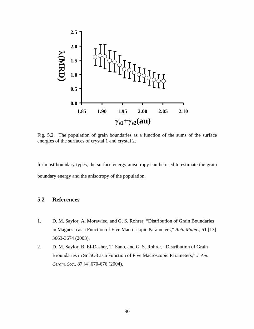
Fig. 5.2. The population of grain boundaries as a function of the sums of the surface energies of the surfaces of crystal 1 and crystal 2.

0.0

0.5

1.0

1.5

2.0

2.5

1.85 1.90 1.95 2.00 2.05 2.10

λ(MR

D)

γs1+γs2(au)

for most boundary types, the surface energy anisotropy can be used to estimate the grain

boundary energy and the anisotropy of the population.

5.2 References

1. D. M. Saylor, A. Morawiec, and G. S. Rohrer, “Distribution of Grain Boundaries

in Magnesia as a Function of Five Macroscopic Parameters,” Acta Mater., 51 [13]

3663-3674 (2003).

2. D. M. Saylor, B. El-Dasher, T. Sano, and G. S. Rohrer, “Distribution of Grain

Broundaries in SrTiO3 as a Function of Five Macroscopic Parameters,” J. Am.

Ceram. Soc., 87 [4] 670-676 (2004).

90

6. Grain Growth Experiments

6.1 Grain Size Distributions

The nucleation limited coarsening theory1 predicts that in a system of completely

dispersed grains in a liquid phase, the defective grains grow at the expense of the small

grains. But as explained in Chapter 1, the contiguity of the actual microstructure will

allow grain growth to occur.

To calculate the rates of grain growth without the effects of liquid, single-phase

polycrystalline SrTiO3 samples were prepared. The sample preparation methods were

identical to that described in Section 3.1.1. After sintering under vacuum for 25 hours at

800°C, the samples were annealed at 1500°C for 0, 5, 10, 15, and 24 hours (ramp rate of

5°C/min). Each sample was lapped, polished, and thermally grooved as described in

Fig. 6.1. A SEM image of the 24 h sample. In addition to flaws from grain pull-out during polishing, there is some porosity.

91

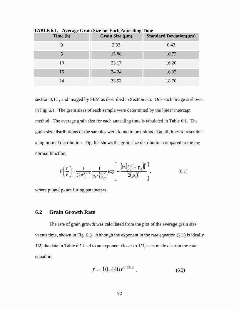
TABLE 6.1. Average Grain Size for Each Annealing Time Time (h) Grain Size (µm) Standard Deviation(µm)

0 2.33 0.43

5 15.88 10.72

10 23.17 16.20

15 24.24 16.32

24 33.53 18.70

section 3.1.1, and imaged by SEM as described in Section 3.5. One such image is shown

in Fig. 6.1. The grain sizes of each sample were determined by the linear intercept

method. The average grain size for each annealing time is tabulated in Table 6.1. The

grain size distributions of the samples were found to be unimodal at all times to resemble

a log normal distribution. Fig. 6.2 shows the grain size distribution compared to the log

normal function,

( )( )( )( ) ⎥

⎥

⎦

⎤

⎢⎢

⎣

⎡ −−

⋅=⎟

⎠⎞

⎜⎝⎛

21

2

2

12/1 2

lnexp1

)2(1

p

prr

rrpr

rFπ

, (6.1)

where p1 and p2 are fitting parameters.

6.2 Grain Growth Rate

The rate of grain growth was calculated from the plot of the average grain size

versus time, shown in Fig. 6.3. Although the exponent in the rate equation (2.1) is ideally

1/2, the data in Table 6.1 lead to an exponent closer to 1/3, as is made clear in the rate

equation,

3312.0448.10 tr = . (6.2)

92

0h

0

30

60

90

120

0.1 1 10

Normalized grain size

Num

ber

5h

0

30

60

90

120

0.1 1 1

Normalized grain size

Num

ber

0

10h

0

30

60

90

120

0.1 1 10

Normalized grain size

Num

ber

15h

0

30

60

90

120

0.1 1 10

Normalized grain size

Num

ber

24h

0

30

60

90

120

0.1 1 10

Normalized grain size

Num

ber

(b)(a)

(d)(c)

Fig. 6.2. Log normal distribution plotted with the grain size distribution of the (a) 0 h sample, (b) 5 h sample, (c) 10 h sample, (d) 15 h sample, and (e) 24 h sample

(e)

93

y = 10.448x0.3312

R2 = 0.9932

0

10

20

30

40

50

60

0 5 10 15 20 25Time (h)

Gra

in S

ize

( µm

)

Fig. 6.3. A plot of the average grain size over time. The standard deviations are depicted by the error bars.

The reason why the rate follows time to the 1/3 (less than time to the 1/2) is most likely

due to pores and impurities inhibiting growth. This growth law will be compared to the

rate of grain size increase that occurs during coarsening.

6.3. References

1. G. S. Rohrer, C. L. Rohrer, and W. W. Mullins, “Coarsening of Faceted Crystals,”

J. Am. Ceram. Soc. 85[3] 675-682 (2002).

94

7. Morphological Changes During Coarsening

7.1 Results

Microscopic observations of SrTiO3 heated for times from 0 to 50 hours in the

eutectic liquid show that both the average grain size and shape change. Fig. 7.1 shows

AFM images of polished surfaces. The solidified eutectic phase, referred to here as the

liquid phase, appears with a lighter contrast in these images because it polishes at a

slower rate and is topographically higher than the SrTiO3 crystals. While the interfaces

between the SrTiO3 and the liquid are easily identified on these planar sections, it should

also be realized that the SrTiO3 crystals impinge upon each other and form a three

(a) (b)

Fig. 7.1. (a) Sample grains with different interface types for the 0 hour sample. (b) Sample faceted grains in the 24 h sample. Darker shades of gray are SrTiO3 crystals and the lighter gray is the eutectic liquid. Grains with a [100] normal to the sample surface are marked with stars.

Curved grain

2µm 10µm

µm0.1

0

95

dimensional skeletal network. From these typical images, it is clear that at all times

examined, the growth shape of SrTiO3 in liquid contains both curved surfaces and flat

surfaces. The average grain sizes were calculated by the linear intercept method of AFM

images and are listed in Table 7.1. However, it should be noted that the grain sizes were

averaged even for microstructures that appeared bimodal. Hence, it would be

inappropriate to assign any physical significance to these grain sizes, since the averages

are not representative of the population. The accurate grain size distributions are

presented in Chapter 8. The point of presenting these data is to show that increasingly

larger crystals were sampled at later times to determine the average shape.

After annealing at 1500°C, orientations of the SrTiO3 grains in a typical area of

the sample were determined by OIM. Micrographs of the same area were then recorded

by AFM. The faceted interfaces between the grain and the liquid imaged by the AFM

were traced and digitized. At least 2500 boundaries were traced for each sample. 2857

lines were traced from 619 grains for the 0 h, 2917 lines from 388 grains for the 5 h, 2526

lines from 554 grains for 15 h, and 3519 lines from 657 grains for the 24 h sample. The

distributions of SrTiO3 surfaces (λ (n)) for the 0 and 24 h samples are shown in Fig. 7.2.

Table 7.1. Average grain size versus time (by AFM) Time (h) Grain Size (µm)

0 0.08

5 4.2

10 6.5

15 10.2

24 16.0

96

As described in Section 3.6.2, the OIM software can be used to automatically

extract the solid-liquid interface line segments. This is an alternative to manually tracing

(a)

(b)

Fig. 7.2. (a) Distribution of SrTiO3 surfaces in contact with the liquid for the 0 h sample, and (b) for the 24 h sample. Both figures were determined by manual boundary tracing of AFM images.

MRD

MRD

97

boundary segments and it was applied to the data from 5, 10, and 24 h samples. Figure

7.3 shows an example of an OIM reconstructed boundary image that was used to extract

solid-liquid interface boundary segment data. The distributions of SrTiO3 surfaces for

these three data sets are shown in a stereographic projection in Fig. 7.4. Both methods

indicate the same morphological trend. All of the samples showed a relatively high

population of 100 type surfaces and a relatively low population of 111 surfaces. For

the traced data set, the MRD ratio of 100 planes to 110 planes increases from 1.23

for the 0 h sample, to a ratio of 2.30 for the 24 h sample. The automatically extracted

data set has the same increasing trend of the 100 to 110 surface MRD ratio from 1.02

Fig. 7.3. The reconstructed boundary image of the 10 h sample. This image is the same OIM scan as that of Fig. 3.10. The method of reconstruction was described in Section 3.6.2.

155 µm

98

for the 5 h sample, to 1.16 for the 10 h, and to 1.49 for the 24 h sample. Both data sets

also show a preference for planes in the <100> zones. At the earliest times, there are also

(a) (b)

(c)

Fig. 7.4. The data analyzed here were obtained by automatic extraction of grain boundaries from the OIM images. (a) Distribution of SrTiO3 surfaces in contact with the liquid for the 5 h sample. (b) Distribution of SrTiO3 surfaces in contact with the liquid for the 10 h sample. (c) Distribution of SrTiO3 surfaces in contact with the liquid for the 24 h sample.

99

peaks at the 110 positions, but they shrink with time and eventually disappear. As the

SrTiO3 crystals are annealed for longer times, a larger fraction of the surface is bounded

by 100 type interfaces. The tendency for crystals to be bounded by 100 surfaces is

confirmed by the shapes of the crystals in Fig. 7.1, which show examples of crystals that

happen to be aligned so that [100] is nearly perpendicular to the sample plane. These

grains have faceted <100> grain interfaces, while others have curved boundaries. The

curved surfaces are probably faster moving surfaces with higher energies.

7.2 Discussion

As shown in Figs. 7.2 and 7.4, the boundary plane orientation distribution evolves

with annealing time. These results provide a statistical representation of the distribution

of orientations in contact with the liquid. These are the surfaces that are receding or

advancing as a result of the coarsening process and the changes in the area of these

surfaces represent the driving force for coarsening.

Initially, the crystals have distinct 100 and 110 planes. This was observed

for 1500°C anneals up to 5 hours. The peaks at the 110 positions in the stereographic

projections disappear at longer anneal times. The analysis of the sample annealed for 24

h shows that the 100 orientation makes up the largest fraction of area in contact with

the liquid. An isolated crystal, therefore, would be expected to have a cubic shape.

These results agree with the characteristics of the equilibrium crystal shape, including the

curved regions around the 100 surfaces.

100

The changes in the interface distribution reported here can potentially influence

the kinetics of coarsening in several ways. First, we assume that the increase in the area

of the 100 surfaces in contact with the liquid occurs because this is the slowest moving

interface. As the crystal grows faster in other directions, the higher mobility interfaces

disappear and leave behind the slowest interface. Since the 111 and neighboring

orientations have very small areas even at the earliest times, we conclude that these

surfaces have mobilities that are significantly greater than those in the <100> zone and

the 100 surfaces have the minimum mobility.

To validate these findings, templated SrTiO3 single crystal growth experiments

were conducted. Single crystals with (100) and (111) orientations were embedded in 15

vol% liquid - 85 vol% solid SrTiO3 matrix samples. After annealing for 5 h at 1500°C,

the (111) single crystal grew 294 microns in the [111] direction, while the (100) single

crystals grew roughly 170 microns in the [100] direction. These results are tabulated in

Table 7.2. It is clear that the (111) surface grows at a much faster rate than the (001)

orientation. An OIM inverse pole figure map of the (111) crystal cross section is shown

in Fig. 7.5(a) and an OIM inverse pole figure map of a (100) oriented crystal cross

section, showing what appears to be columnar growth, is shown in Fig. 7.5(b).

Table 7.2. Measurements of crystal growth into the matrix Single Crystal Orientation (001) sample 1 (001) sample 2 (111)

Average Growth (µm) 172.24 168.44 294.31

101

Fig. 7.5. (a) An OIM map of the templated (111) single crystal sample. (b) An OIM map of a templated (100) single crystal sample.

Gro

wth

D

irec

tion (b)

Ori

gina

l sin

gle

crys

tal

Gro

wth

dir

ectio

n

Ori

gina

l sin

gle

crys

tal

(a)

102

However observations by Chung and Kang1 of macroscopic SrTiO3 crystals

growing into a matrix of fine grains indirectly suggest that the 110 orientation grows

more slowly than the 100 orientation. Although the origin of this inconsistency is not

clear, it should be noted that several aspects of the prior work differ from the present

circumstances, such as the amount and composition of the liquid, and the defect structure

and composition of the growing crystal. In any case, it can be concluded that as more of

the total interfacial area is made up of the more slowly moving surfaces, the average

growth rate will be diminished. Another factor that affects the coarsening rate is the

change in the average surface energy. If the 100 orientation has the minimum energy,

then the driving force for growth is diminished as this orientation comprises a greater

fraction of the total interfacial area.

7.3 References

1. S.-Y. Chung and S.-J.L. Kang, “Intergranular Amorphous Films and Dislocation

Promoted Grain Growth in SrTiO3,” Acta Mater., 51[8] 2345-2354 (2003).

103

8. Evolution of the Size Distribution During

Coarsening

8.1 Crystal Shapes in Liquid

The motivation for this thesis was to experimentally test the nucleation limited

coarsening theory. The nucleation limited coarsening theory, described in Section 2.6.4,

predicts that below a certain average size, all grains can participate in the coarsening

process. However, when the defect free crystals reach a size where the NEB is

sufficiently larger than available thermal fluctuations, coarsening will be affected.

Because there is no NEB for crystals less than ½ r*, the dissolution of these crystals is

not limited. Hence these defect free crystals will dissolve and supply the material that

allows the defective grains to grow. During this coarsening period, the grain size

distribution is bimodal and the number density of abnormal grains is constant. When all

of the small, defect free grains are consumed, the larger defective grains will no longer

have any advantage and normal coarsening will occur, exhibiting a unimodal grain size

distribution. Hence the main predictions of the theory are, 1) transient bimodal grain size

distribution exists, 2) the number density of abnormal grains during the bimodal regime is

constant, 3) the small grains do not coarsen, and 4) the number density of the small grains

decreases during the bimodal regime. To test these theoretical predictions, accurate

measurements of the crystal size and shape distributions as a function of time are needed.

From those measurements, the number densities of abnormal and small grains will be

104

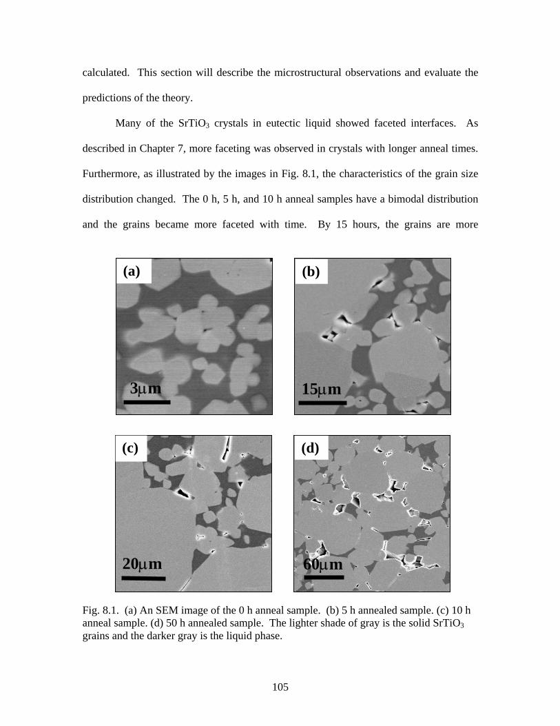
calculated. This section will describe the microstructural observations and evaluate the

predictions of the theory.

Many of the SrTiO3 crystals in eutectic liquid showed faceted interfaces. As

described in Chapter 7, more faceting was observed in crystals with longer anneal times.

Furthermore, as illustrated by the images in Fig. 8.1, the characteristics of the grain size

distribution changed. The 0 h, 5 h, and 10 h anneal samples have a bimodal distribution

and the grains became more faceted with time. By 15 hours, the grains are more

Fig. 8.1. (a) An SEM image of the 0 h anneal sample. (b) 5 h annealed sample. (c) 10 h anneal sample. (d) 50 h annealed sample. The lighter shade of gray is the solid SrTiO3 grains and the darker gray is the liquid phase.

60µm

(d)(c)

20µm

3µm

(a) (b)

15µm

105

TABLE 8.1. Average grain size over time (by SEM) Time (h) Grain Size (µm)

0 1.22 3 4.73

5 6.78

10 15.93

15 21.39

24 23.80

50 35.37

homogenous in size, and a distinct bimodal distribution no longer exists. The sample

annealed for 50 h continues in this trend and the grain size distribution is unimodal. At

all annealing times, there were some grains several times larger than the others. To

quantify what is evident in Fig. 8.1, grain sizes were determined from SEM images by the

linear intercept method and are listed in Table 8.1.

The frequency of normalized grain sizes for the 24 h sample is compared to the

ideal LSW distribution, shown in Fig 8.2. The 24 h data set was scaled by a constant to

match the area under the curve of the LSW distribution. The predicted distribution is

inconsistent with the experimental data. The LSW distribution has a maximum grain size

of 3/2 r , which does not agree with the experimental result, where the maximum reduced

grain size was 5.65. Fig. 8.3 was obtained by plotting the frequency versus the reduced

grain size. The curves are not consistently self-similar like the grain growth distributions

shown in Fig. 6.2.

When the volume percentages of grain sizes were analyzed, unlike the grain

growth experiment, the coarsening experiments showed bimodal distributions. Samples

annealed between 0 and 10 hours exhibited bimodal grain size distributions, but the

106

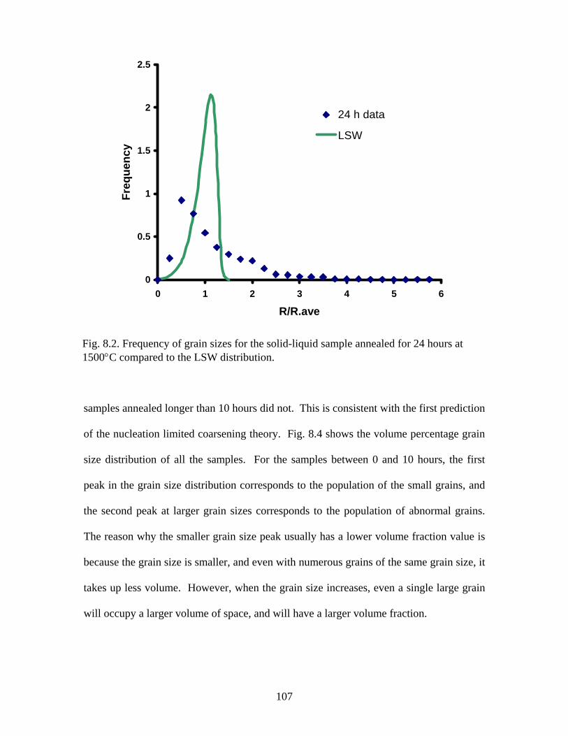
samples annealed longer than 10 hours did not. This is consistent with the first prediction

of the nucleation limited coarsening theory. Fig. 8.4 shows the volume percentage grain

size distribution of all the samples. For the samples between 0 and 10 hours, the first

peak in the grain size distribution corresponds to the population of the small grains, and

the second peak at larger grain sizes corresponds to the population of abnormal grains.

The reason why the smaller grain size peak usually has a lower volume fraction value is

because the grain size is smaller, and even with numerous grains of the same grain size, it

takes up less volume. However, when the grain size increases, even a single large grain

will occupy a larger volume of space, and will have a larger volume fraction.

0

0.5

1

1.5

2

2.5

0 1 2 3 4 5

R/R.ave

Freq

uenc

y

6

24 h data

LSW

Fig. 8.2. Frequency of grain sizes for the solid-liquid sample annealed for 24 hours at 1500°C compared to the LSW distribution.

107

0 hour

0

60

120

180

240

0.1 1 10

r/r.average

Freq

uenc

y

3 hour

0200400600800

1000

0.1 1 10

r/r.average

Freq

uenc

y

5 hour

0

800

1600

2400

3200

0.1 1 10

r/r.average

Freq

uenc

y

10 hour

0

300

600

900

1200

0.1 1 10

r/r.average

Freq

uenc

y

15 hour

0

200

400

600

800

1000

0.1 1 10

r/r.average

Freq

uenc

y

24 hour

0

200

400

600

0.1 1 10

r/r.average

Freq

uenc

y

50 hour

070

140210280350

0.1 1 10r/r.average

Freq

uenc

y Fig. 8.3. Frequency of grain size versus the normalized grain size for the solid-liquid samples annealed at 1500°C for (a) 0 hours, (b) 3 hours, (c) 5 hours, (d) 10 hours, (e) 15 hours, (f) 24 hours, and (g) 50 hours.

(g)

(f)(e)

(d)(c)

(b)(a)

108

0 hour

0

2

4

6

8

0.1 1 10

Grain Size (µm)

Volu

me

%

3 hour

0

2

4

6

8

0.1 1 10 100

Grain Size (µm)

Volu

me

%

5 hour

0

2

4

6

0.1 1 10 100Grain Size (µm)

Volu

me

%

10 hour

0

2

4

6

0.1 1 10 100Grain Size (µm)

Volu

me

%

15 hour

0

2

4

6

0.1 1 10 100

Grain Size (µm)

Volu

me

%

24 hour

0

2

4

6

0.1 1 10 100

Grain Size (µm)

Volu

me

%

50 hour

0

2

4

6

0.1 1 10 100

Volu

me

% Fig. 8.4. Grain size distribution of the solid-liquid sample annealed at 1500°C for (a) 0 hours, (b) 3 hours, (c) 5 hours, (d) 10 hours, (e) 15 hours, (f) 24 hours, and (g) 50 hours.

(a) (b)

(c) (d)

(e) (f)

(g)

109

0

2

4

6

0.1 1 10r/r.ave

Volu

me

%

0

2

4

6

0.1 1 10r/r.critical

Volu

me

%

Fig. 8.5. Figure (a) is the volume percentages of grain sizes for the 5 h single-phase sample. Figure (b) is the volume percentages of grain sizes for the 5 h two-phase sample.

(b)

(a)

110

The grain sizes from the single-phase grain growth experiments did not show any

bimodal grain size distributions. Fig. 8.5 shows an example of the volume fraction

versus grain size in the coarsening and grain growth experiments. The 5 h grain growth

volume fraction versus grain size plot in Figure 8.5(a) shows a unimodal distribution,

while Figure 8.5(b), the 5 h coarsening volume percentage versus grain size shows two

peaks; a smaller peak around 0.6 and a larger peak at roughly 7. The observed

distributions are clearly inconsistent with the LSW theory. The maximum grain size

found to be larger than 3/2 r , as mentioned earlier. In addition, although the LSW theory

predicts grain size distributions to be constant with time, the experimental results show

that the distribution changes with time.

8.2 Results of the Grain Population Based on Size

These experiments were based on the idea that the large grains and the smallest

grains evolve by different mechanisms. To analyze their populations separately, the

crystals were classified as abnormal grains (grains in the second peak of the grain size

distribution) and small grains (grains in the first peak of the grain size distribution.

Bimodal distributions were observed between 0 and 10 hours. Hence the analysis will be

on samples from this time frame. This section will address the evolution of the grains in

both populations, starting with the abnormal grains.

Fig. 8.6 shows the median grain size of abnormal grains (listed in Table 8.1) over

time. These grain size measurements closer to the t1/3 relation than the t1/2 relation.

Though inconclusive, this suggests that the abnormal grains could be coarsening by the

diffusion limited mechanism and attachment/detachment kinetics are not limiting growth.

111

This is what is expected for crystals with persistent step sources according to the

nucleation limited coarsening theory.

To test the second prediction of the nucleation limited coarsening theory, the

volume density of abnormal grains was calculated. During the abnormal coarsening

regime, the number of abnormal grains is predicted to stay approximately constant. The

volume density of abnormal grains, Nv, was determined from planar SEM images, by

using the following stereological result to correct for the bias introduced by observations

from a single section1,

Nv = NA/d, (8.1)

y = 16.149x0.2421

R2 = 0.9711

0

10

20

30

40

50

60

0 2 4 6 8Time (h)

Gra

in s

ize

( µm

)

10

Fig. 8.6. The median abnormal grain sizes over time plotted with standard deviation error bars. The trend line equation has time to the power of 0.24.

112

where NA is the number of abnormal grains per area and d is the average diameter of the

abnormal grains. The volume density as a function of time is plotted in Fig 8.7, where

the standard deviations are represented by the error bars. As formulated in Eq. (8.1), the

points are the observed number of abnormal grains per area, divided by the average

diameter of the abnormal grains of that sample. During the abnormal coarsening regime

from 0 to 5 hours, the volume density of abnormal grains is constant within experimental

uncertainty. At 10 hours, the bimodal grain size distribution is nearly unimodal (Fig.

8.4(d)) and hence the volume density is lower than those of 0 to 5 hours. When an

0.0E+00

5.0E-05

1.0E-04

1.5E-04

2.0E-04

2.5E-04

0 5 10 15

Time (h)

Volu

me

Den

sity

(Num

ber/ µ

m3 )

Fig. 8.7. Volume density of abnormal grains versus annealing time. The error bars indicate the standard deviation.

113

approximately unimodal distribution returns at 15 hours, the volume density is reduced.

This abnormal grain volume density relation was predicted by the nucleation limited

coarsening theory. Another aspect that is consistent with this theory, is that after the

abnormal coarsening regime, a unimodal distribution is observed.

The third prediction of the nucleation limited coarsening theory is that these small

grains would stop coarsening, dissolve, and be incorporated into the large grains.

Calculations of the average sizes of the small grains show that they continue to grow (see

Table 8.2). These are different from the average grain sizes in Table 7.1, which were

measured by AFM. While the measurements by the linear intercept method of AFM

images selectively samples crystals in the AFM field of view, it overlooks the larger

crystals and has a much smaller sampling area. The measurements from the SEM scans

incorporate a larger area, and can be more accurate by using multiple magnifications.

Small grain sizes measured from SEM images plotted as a function of the anneal time is

shown in Fig. 8.8. This is comparable to the observations by Rehrig et al.2 (see Fig. 8.9)

who saw a small increase in grain size for the smaller crystals. The increase in the

SrTiO3 small grain sizes is within the standard deviation of Rehrig et al.’s results. The

cause of the growth is believed to be not by coarsening, but by grain growth. This

hypothesis will be investigated further in Chapter 9.

The change in volume density over time for the small grains is consistent with the

TABLE 8.2. Sizes of the small grains over time Anneal time (H) 0 3 5 10

Grain Size (µm) 0.79 2.49 3.48 5.95

114

0

2

4

6

8

10

0 2 4 6 8 10 1

Time (h)

Gra

in S

ize

( µm

)

2

Fig. 8.8. The sizes of the small grains versus time. The error bars represent the standard deviation.

fourth prediction of the nucleation limited coarsening theory. Initially there is a large

density of small grains, but over time, the density decreases (see Fig. 8.10).

The four main predictions of the nucleation limited coarsening theory have been

examined. The experimental results are consistent with the predictions. The only

uncertain results are the growth mechanism of the small grains. This will be addressed in

the next chapter.

115

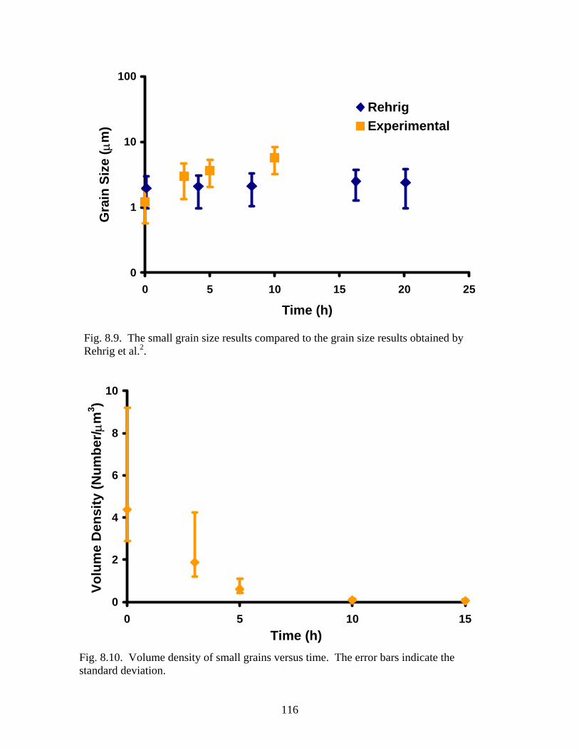
0

1

10

100

0 5 10 15 20 25

Time (h)

Gra

in S

ize

( µm

)RehrigExperimental

Fig. 8.9. The small grain size results compared to the grain size results obtained by Rehrig et al.2.

0

2

4

6

8

10

0 5 10 15Time (h)

Volu

me

Den

sity

(Num

ber/ µ

m3 )

Fig. 8.10. Volume density of small grains versus time. The error bars indicate the standard deviation.

116

8.3 References

1. J. C. Russ, Practical Rheology; p. 54. Plenum Press, New York, 1986.

2. P. W. Rehrig, G. L. Messing, and S. Trolier-McKinstry, “Templated Grain

Growth of Barium Titanate Single Crystals,” J. Am. Ceram. Soc., 83[11] 2654-

2660 (2000).

117

9. Kinetics of Growth

9.1 Comparison with Grain Growth Rate

In Section 8.2, the small grains were found to grow with time. The mechanism for

this growth is believed to be by grain growth. To verify this hypothesis and the

suggestion that the abnormal grain are coarsening, the grain growth rates were compared

to the coarsening rates. The analysis of the abnormal grains will be discussed first.

The grains in the single-phase sample can only grow by grain growth. The average

grain size of these grains increased at a rate of time to the 1/3, or the equation,

3312.0448.10 tr = . (9.1)

Compared to the small grains’ coarsening rate in the two-phase sample, the single-phase

grain growth rate for average sized grains was faster. However, the largest grain sizes in

the two-phase sample showed the opposite relation. The abnormal grains in the two-

phase sample grew at a faster rate than the average grains in the single-phase sample.

These growth rate comparisons are plotted in Fig. 9.1. The two-phase sample having a

faster growth or coarsening rate for the abnormal grains is evident in Fig. 8.5, where the

maximum grain size for the two-phase sample is larger than the maximum grain size in

the single-phase sample. However for a given annealing time, the average sized grains in

the single-phase sample were larger than the average sized grains in the two-phase

sample. But as stated earlier, the abnormal grains of the two-phase sample are larger than

the largest grains in the single-phase sample. This indicates that in the two-phase

samples, the abnormal grains are coarsening and not growing by grain growth. If the

abnormal grains were growing by grain growth, since the grain growth rate is slower, the

118

abnormal grains will be no bigger than the largest grains in the single-phase samples.

However that was not the case.

Recent observations of abnormal grain growth in polycrystalline alumina by

MacLaren et al1 and Dillon and Harmer2, suggests impurities play a large role in grain

boundary mobility. Silica and yttria impurities accumulated at some rough alumina grain

boundaries, causing an impurity induced structural transition. At some critical impurity

concentration, when the samples were annealed above 1550°C, an amorphous layer, less

than a nanometer thick, developed between the grain boundaries. This transition is

believed to be the cause of the increase in the mobility of those grain boundaries. This

structural transition could be a reasonable explanation for abnormal grain growth in the

polycrystalline case, but for crystals with flat interfaces coarsening in 15 volume %

liquid, the impurity concentration argument for abnormal coarsening is unlikely, since

excess liquid is present at all stages.

Finally, the appearance of grains with flat facets in contact with the liquid

suggests that some of these surfaces, such as those with the 100 orientation, are

singular. Models for nucleation limited coarsening described in Section 2.6.4 suggest

that such interfaces should be immobile unless a step-generating defect, such as a screw

dislocation, exists at the surface3, 4. According to coarsening models based on these

assumptions, the only crystals that can grow are those containing a defect. Because

crystals less than ½ r* can shrink without a barrier, some of the ideal crystals bounded by

singular surfaces are able to supply material to sustain the growth of larger crystals with

defects4. For ceramics, we can take the approximate dislocation density to be 106/cm2.

Therefore, there is one dislocation in a crystal with a 1 µm diameter. We note that in the

119

0

20

40

60

80

0 2 4 6 8 10Time (h)

Gra

in S

ize

( µm

)Two-phase Abnormal Grains

Two-phase Small Grains

Single-phase Grain Growth Average

Fig. 9.1. A plot of the average grain growth rate versus coarsening rates for the abnormal grains and the small grains.

present case, by considering volume conservation, coarsening from an average size of 0.8

µm to 16 µm means that roughly 1 in 8000 of the crystals in the initial population persist

throughout growth. It is reasonable to suspect that step-generating defects would be

found in crystals prepared by ball milling with at least this frequency.

The results of the small grains in the two-phase sample showed that they are

growing slower than the average grains in the single-phase sample. This supports the

possibility that the smaller grains’ growth mechanism is dominated by grain growth. The

120

maximum growth rate for the small grains is the grain growth rate of the average grains

in the single-phase sample. The growth rate being slower than the maximum rate is

reasonable, since the contiguity of the two-phase sample is less than the single-phase

sample. But to be certain, the grain sizes of smaller grains, calculated to have grown by

grain growth affected by contiguity, will be compared with the experimental small grain

sizes.

9.2 Calculated Small Grain Sizes

To determine how much of the surface area of small grains are bound by other solid

crystals, and hence allowing for the possibility of grain growth, the solid phase contiguity

was calculated. The solid phase contiguity is the ratio of solid-solid interface area over

all the interface areas5, 6. Using the experimental measurements of the solid-solid and

solid-liquid interface line segments, the contiguity can be calculated by the equation7,

[ ]∑∑

+=

)()(2)(2

//

/

lsss

ss

LengthLengthLength

Contiguity (9.2)

where s/s indicates solid-solid interfaces and s/l indicates solid-liquid interfaces. In the

OIM scans, if a grain appeared to be located next to another grain, the boundary was

considered to be a solid-solid grain boundary. If the grain had a neighbor with Euler

Table 9.1. Calculated versus experimental small grain sizes Time (h) Experimental (µm) Calculated- only

grain growth (µm) Calculated- grain growth

and coarsening (µm) 0 0.79 0.72 2.17

3 2.49 4.75 9.44

5 3.48 5.63 10.82

10 5.95 7.08 13.02

121

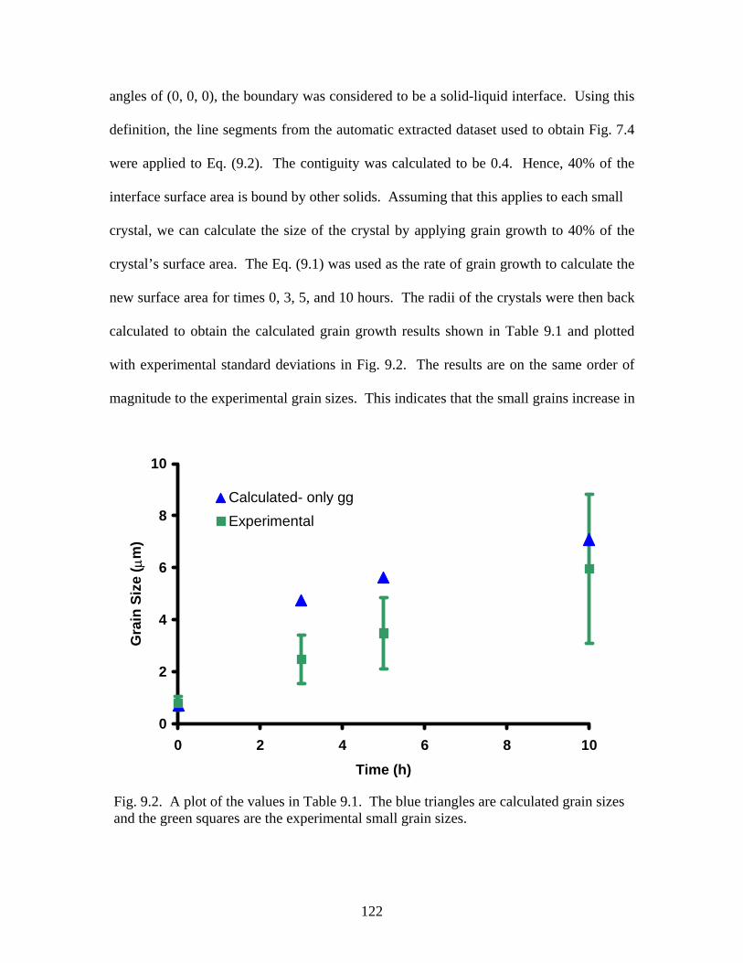
angles of (0, 0, 0), the boundary was considered to be a solid-liquid interface. Using this

definition, the line segments from the automatic extracted dataset used to obtain Fig. 7.4

were applied to Eq. (9.2). The contiguity was calculated to be 0.4. Hence, 40% of the

interface surface area is bound by other solids. Assuming that this applies to each small

crystal, we can calculate the size of the crystal by applying grain growth to 40% of the

crystal’s surface area. The Eq. (9.1) was used as the rate of grain growth to calculate the

new surface area for times 0, 3, 5, and 10 hours. The radii of the crystals were then back

calculated to obtain the calculated grain growth results shown in Table 9.1 and plotted

with experimental standard deviations in Fig. 9.2. The results are on the same order of

magnitude to the experimental grain sizes. This indicates that the small grains increase in

0

2

4

6

8

10

0 2 4 6 8Time (h)

Gra

in S

ize

( µm

)

10

Calculated- only ggExperimental

Fig. 9.2. A plot of the values in Table 9.1. The blue triangles are calculated grain sizes and the green squares are the experimental small grain sizes.

122

size at a rate that is consistent with the grain growth rate. When coarsening is

incorporated into the calculations by assuming that the small grain has a defect and hence

40% of the crystal surface is undergoing grain growth and 60% of the crystal surface is

coarsening by the rate of coarsening determined from the abnormal grains, the calculated

grain sizes increased by over 85%. The calculated grain sizes incorporating grain growth

and coarsening mechanisms are also shown in Table 9.1. When 60% of the surface area

is considered to be coarsening, since the coarsening rate is much faster than the grain

growth rate, the effect is significant. Thus, we can conclude that the small grains are

growing by grain growth, and not coarsening, which is consistent with the fourth

prediction of the nucleation limited coarsening theory as listed in Section 8.1.

9.3 References

1. I. McLaren, R. M. Cannon, M. A. Gülgün, R. Voytivych, N. Popescu-Pogrion, C.

Scheu, U. Täffner, and M. Rühle, “Abnormal Grain Growth in Alumina:

Synergistic Effects of Yttria and Silica,” J. Amer. Ceram. Soc., 86[4] 650-659

(2003).

2. S. Dillon and M. P. Harmer, [personal communication].

3. B.W. Sheldon and J.Rankin, “Step-Energy Barriers and Particle Shape Changes

during Coarsening,” J. Amer. Ceram. Soc., 85[3] 683-690 (2002).

4. G. S. Rohrer, C. L. Rohrer, and W. W. Mullins, “Coarsening of Faceted Crystals,”

J. Am. Ceram. Soc. 85[3] 675-682 (2002).

5. J. Gurland, “An Estimate of Contact and Contiguity of Dispersions in Opaque

Samples,” Trans. Metall. Soc. AIME, 236[5] 642-646 (1966).

123

6. R. M. German, “The Contiguity of Liquid Phase Sintered Microstructures,”

Metall. Trans. A, 16A[7] 1247-1252 (1985).

7. E. Underwood, Quantitative Stereology; Addison-Wesley, New York, 1970.

124

10. Conclusions

To test the nucleation limited coarsening theory, the SrTiO3 system was studied.

A comprehensive investigation of the surface energy anisotropy, grain boundary plane

distribution, crystal shapes, grain size distribution, and kinetics of SrTiO3 grains in excess

liquid was conducted.

The thermal groove method was used to determine the surface energy anisotropy

of SrTiO3 in air at 1400°C. In this system, the 100 surfaces had the lowest energy,

followed by 110 and 111 surfaces. Surfaces vicinal to 100 and 110 surfaces

were also on the equilibrium crystal shape. The grain boundary population was found to

be inversely correlated to the sum of the energies of the surfaces adjoining the boundary.

In other words, even in dense polycrystals, grain surfaces tend to be terminated by low

energy 100 planes.

The tendency to terminate crystals by 100 surfaces was also observed in the

coarsening experiment. The observed habit planes are not indications of surfaces on the

Wulff shape, but simply indicate the surfaces that are part of the growth shape during

coarsening. The crystals coarsening in the eutectic liquid had large areas of 100 planes

and some 110 planes. Unlike the solid-vapor equilibrium shape, the coarsening grains

did not exhibit a preference for 111 surfaces. In fact, the 111 planes were the least

observed. As the crystals coarsened, the frequency of 110 plane observations

decreased and the frequency of 100 plane observations increased.

125

The results from the study of SrTiO3 coarsening in a eutectic liquid are

inconsistent with LSW’s predictions that the maximum grain size is 3/2 r . On the other

hand, the results support the nucleation limited coarsening theory. At the earlier times of

coarsening, the grain size distribution appeared bimodal. The samples annealed for 3, 5

and 10 hours exhibited a continued bimodal distribution of grains. A more homogeneous

grain size returned after annealing for 15 hours. The results showed that the abnormal

grains were coarsening faster than the single-phase grains growing by grain growth. This

indicates that these grains are coarsening and have no nucleation barriers. In addition, the

result of the volume fraction of abnormal grains was consistent with that predicted by the

nucleation limited coarsening theory.

The continued growth of the small grains was due to grain growth. Application of

single-phase grain growth rate to the solid-solid interface area of the small grains in the

two-phase sample resulted in a comparable grain size to those determined by

experiments. The rate of growth for the small grains was slower than those of abnormal

grains and the single-phase grains. The small grains’ growth rate is consistent with the

grain growth mechanism limited by reduced contiguity. This is still consistent with the

nucleation limited coarsening theory, in that abnormal coarsening is occurring due to a

population of defective grains growing by the coarsening mechanism, while a population

of defect free crystals are growing by grain growth but also being consumed by the

defective grains by capillarity forces. When the small, defect free crystals are all

consumed, a unimodal grain size distribution develops.

126

11. Future Work

11.1 Monte Carlo Simulation

In Chapter 9, the continued growth of small grains was explained by grain

growth. However the calculated predictions of grain sizes increasing by grain growth and

coarsening, affected by the reduced contiguity, are primitive. Monte Carlo simulations

with initial microstructures from the experimental data will be used to better estimate the

grain sizes.

The 2-D Monte Carlo simulation of microstructural evolution during coarsening

will be based on the work by Tikare and Cawley1. To mimic the coarsening and growth

mechanisms of the samples, grain growth will also be applied. If the randomly chosen

site is a solid and the chosen neighbor is liquid, or vice versa, coarsening will occur. If

however both the chosen site and the neighbor are solids, grain growth will occur.

The initial microstructure required for the simulations are based on the OIM scans

of the coarsening samples. Using the TexSEM software’s Grain File output, the liquid

phase with artificial Euler angles of (0, 0, 0) is given the grain id value of –1. The

location of the grains and liquid are based on the x, y coordinates given in the Grain File

and converted to pixel locations. Since for Monte Carlo simulations, the microstructure

must be periodic, a contingency will be placed so that if the randomly chosen site is at the

edge or corner of the microstructure, the choices of the neighbor sites will be forced

within the microstructure.

127

In addition, 2-D Monte Carlo simulation of grain growth will be conducted to

compare the difference between the simulated rate of the combined coarsening and grain

growth of the two-phase system and the simulated rate of grain growth of the single-

phase system with pores.

11.2 Grain Boundary Wetting

In addition to the Monte Carlo simulations, other work that will complete the

thesis is to analyze the grain boundaries by transmission electron microscopy (TEM).

We have assumed that grains that are touching other grains are bound by solid-solid

boundaries. However we do not know for certain if there is a nanometer thick film of

liquid between the grains. The results of a TEM analysis could affect the contiguity and

the grain growth argument for the small grains.

11.3 Experiments Without Contiguity Effects

Coarsening experiments with microstructures that closely resemble the theoretical

microstructure can be conducted. This micro designed technique was used by Kitayama

et al.2 and requires lithographic patterning of pores into a single crystal. The location of

the etched pores can be controlled such that contiguity is not a factor. Another single

crystal is bonded over the pores, to transform the pores into cavities. Coarsening

experiments of these negative grains can be conducted and locations of defects

determined by etching the surfaces of the surfaces of the pores.

128

11.4 References

1. V. Tikare and J. D. Cawley, “Application of the Potts Model to Simulation of

Ostwald Ripening,” J. Am. Ceram. Soc., 81[3] 485-491 (1998).

2. M. Kitayama, T. Narushima, and A. M. Glaeser, “The Wulff Shape of Alumina:

II, Experimental Measurements of Pore Shape Evolution Rates,” J. Am. Ceram.

Soc., 83 [10] 2572-83 (2000).

129

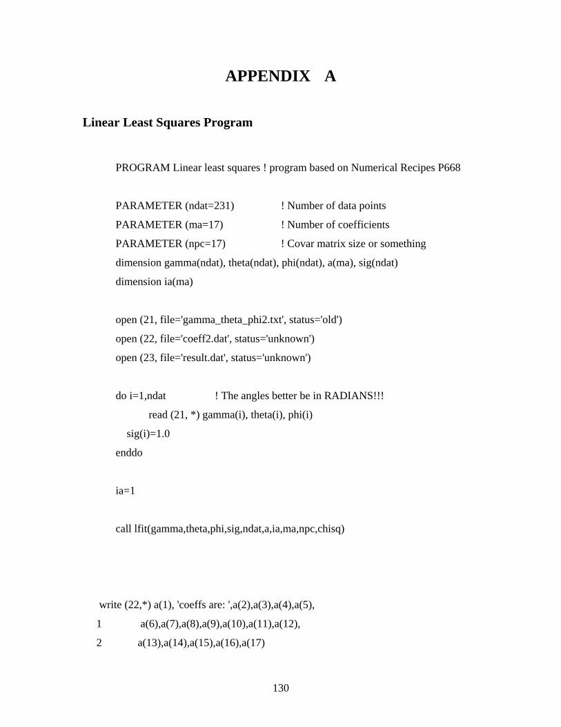
APPENDIX A Linear Least Squares Program

PROGRAM Linear least squares ! program based on Numerical Recipes P668

PARAMETER (ndat=231) ! Number of data points

PARAMETER (ma=17) ! Number of coefficients

PARAMETER (npc=17) ! Covar matrix size or something

dimension gamma(ndat), theta(ndat), phi(ndat), a(ma), sig(ndat)

dimension ia(ma)

open (21, file='gamma_theta_phi2.txt', status='old')

open (22, file='coeff2.dat', status='unknown')

open (23, file='result.dat', status='unknown')

do i=1,ndat ! The angles better be in RADIANS!!!

read (21, *) gamma(i), theta(i), phi(i)

sig(i)=1.0

enddo

ia=1

call lfit(gamma,theta,phi,sig,ndat,a,ia,ma,npc,chisq)

write (22,*) a(1), 'coeffs are: ',a(2),a(3),a(4),a(5),

1 a(6),a(7),a(8),a(9),a(10),a(11),a(12),

2 a(13),a(14),a(15),a(16),a(17)

130

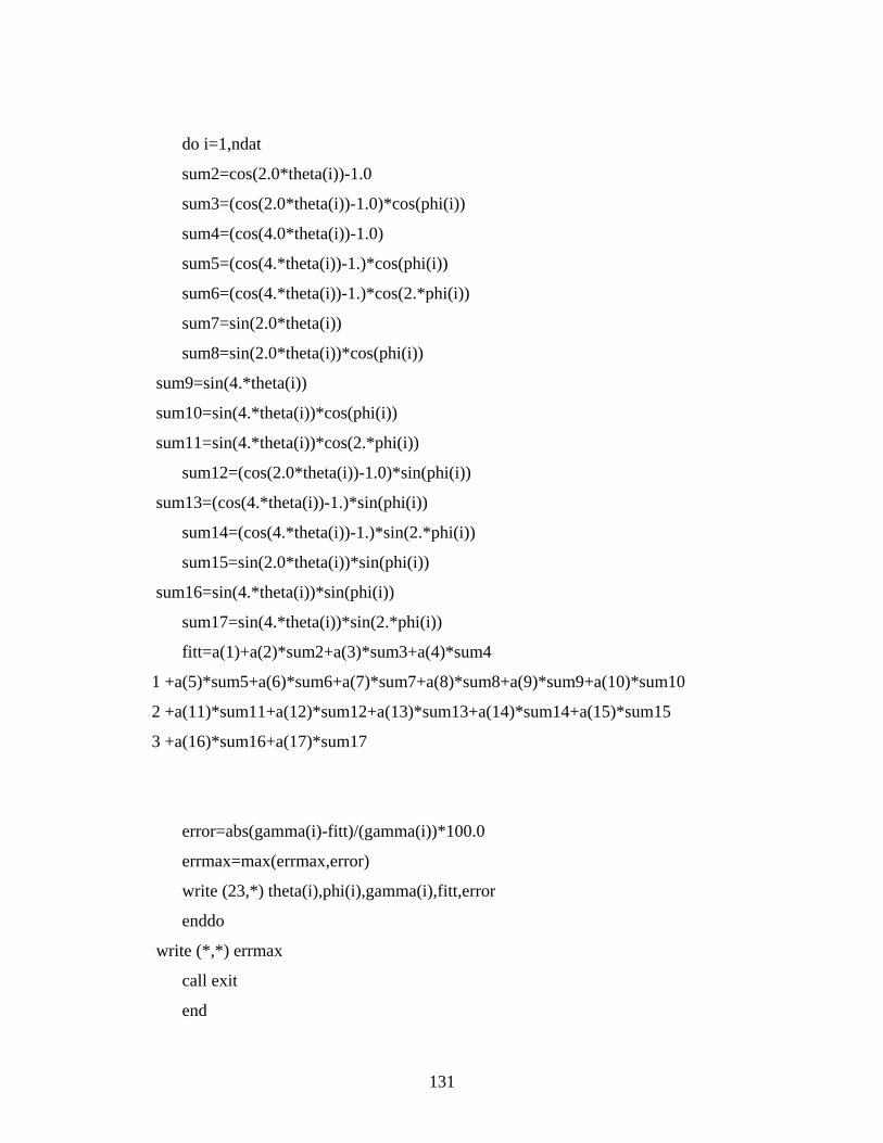
do i=1,ndat

sum2=cos(2.0*theta(i))-1.0

sum3=(cos(2.0*theta(i))-1.0)*cos(phi(i))

sum4=(cos(4.0*theta(i))-1.0)

sum5=(cos(4.*theta(i))-1.)*cos(phi(i))

sum6=(cos(4.*theta(i))-1.)*cos(2.*phi(i))

sum7=sin(2.0*theta(i))

sum8=sin(2.0*theta(i))*cos(phi(i))

sum9=sin(4.*theta(i))

sum10=sin(4.*theta(i))*cos(phi(i))

sum11=sin(4.*theta(i))*cos(2.*phi(i))

sum12=(cos(2.0*theta(i))-1.0)*sin(phi(i))

sum13=(cos(4.*theta(i))-1.)*sin(phi(i))

sum14=(cos(4.*theta(i))-1.)*sin(2.*phi(i))

sum15=sin(2.0*theta(i))*sin(phi(i))

sum16=sin(4.*theta(i))*sin(phi(i))

sum17=sin(4.*theta(i))*sin(2.*phi(i))

fitt=a(1)+a(2)*sum2+a(3)*sum3+a(4)*sum4

1 +a(5)*sum5+a(6)*sum6+a(7)*sum7+a(8)*sum8+a(9)*sum9+a(10)*sum10

2 +a(11)*sum11+a(12)*sum12+a(13)*sum13+a(14)*sum14+a(15)*sum15

3 +a(16)*sum16+a(17)*sum17

error=abs(gamma(i)-fitt)/(gamma(i))*100.0

errmax=max(errmax,error)

write (23,*) theta(i),phi(i),gamma(i),fitt,error

enddo

write (*,*) errmax

call exit

end

131

! -----------------------------------------------------------------

Subroutine lfit(gamma,theta,phi,sig,ndat,a,ia,ma,npc,chisq)

Parameter (MMAX=17)

Dimension ia(ma),a(ma),covar(npc, npc),sig(ndat)

Dimension theta(ndat),phi(ndat),gamma(ndat)

Integer i, j, k, l, m, mfit

Real sig2i, sum, wt, ym

Dimension afunc(MMAX), beta(MMAX)

mfit=0

do j=1, ma

if (ia(j).ne.0) mfit=mfit+1

enddo

if (mfit.eq.0) pause 'lfit: no parameter to be fitted'

covar=0.

beta=0.

do i=1, ndat

call choad(afunc,theta(i),phi(i))

ym=gamma(i)

if (mfit.lt.ma) then

do j=1, ma

if (ia(j).eq.0) ym=ym-a(j)*afunc(j)

enddo

endif

132

sig2i=1./sig(i)**2

j=0

do l=1, ma

if (ia(l).ne.0) then

j=j+1

wt=afunc(l)*sig2i

k=0

do m=1,l

if (ia(m).ne.0) then

k=k+1

covar(j, k) = covar(j, k)+wt*afunc(m)

endif

enddo

beta(j) = beta(j)+ym*wt

endif

enddo

enddo

do j=2, mfit

do k=1, j-1

covar(k, j) = covar(j, k)

enddo

enddo

call gaussj(covar, mfit, npc, beta, 1, 1)

j=0

do l=1, ma

133

if (ia(l).ne.0) then

j=j+1

a(l) = beta(j)

endif

write (*,*) a

enddo

chisq=0.

do i=1, ndat

call choad (afunc,theta(i),phi(i))

sum=0.

do j=1, ma

sum=sum+a(j)*afunc(j)

enddo

chisq=chisq+((gamma(i)-sum)/sig(i))**2

enddo

! call covsrt(covar, npc, ma, ia, mfit) ! Not bothering w/ this subroutine

return

End

! --------------------------------------------------------------

Subroutine covsrt(covar, npc, ma, ia, mfit)

Integer ma, mfit, npc, ia(ma)

Real*4 covar(npc, npc)

Integer i, j, k

134

Real*4 swap

do i=mfit+1, ma

do j=1, i

covar(i, j)=0

covar(j, i)=0

enddo

enddo

k=mfit

do j=ma, 1, -1

if (ia(j).ne.0) then

do i=1, ma

swap=covar(i, k)

covar(i, k)=covar(i, j)

covar(i, j)=swap

enddo

do i=1, ma

swap=covar(k, i)

covar(k, i)=covar(j, i)

covar(j, i)=swap

enddo

k=k-1

endif

enddo

return

end

! ---------------------------------------------------------------

135

Subroutine gaussj(covar, mfit, npc, beta, m, mp)

PARAMETER (NMAX=17)

Integer mfit, npc, m, mp

Real covar(npc,npc), beta(npc,mp)

Integer i,icol,irow,j,k,l,ll

DIMENSION indxc(NMAX),indxr(NMAX),ipiv(NMAX)

Real big, dum, pivinv

do j=1, mfit

ipiv(j)=0

enddo

do i=1, mfit

big=0.

do j=1, mfit

if(ipiv(j).ne.1) then

do k=1, mfit

if (ipiv(k).eq.0) then

if (abs(covar(j, k)).ge.big) then

big=abs(covar(j, k))

irow=j

icol=k

endif

else if (ipiv(k).gt.1) then

pause 'singular matrix in gaussj'

endif

enddo

endif

136

enddo

ipiv(icol)=ipiv(icol)+1

if (irow.ne.icol) then

do l=1, mfit

dum=covar(irow, l)

covar(irow, l)=covar(icol,l)

covar(icol, l)=dum

enddo

do l=1, m

dum=beta(irow, l)

beta(irow, l)=beta(icol,l)

beta(icol, l)=dum

enddo

endif

indxr(i)=irow

indxc(i)=icol

if (covar(icol, icol).eq.0.) pause 'singular matrix in gaussj'

pivinv=1./covar(icol, icol)

covar(icol, icol)=1.

do l=1, mfit

covar(icol, l)=covar(icol, l)*pivinv

enddo

do l=1, m

beta(icol, l)=beta(icol, l)*pivinv

enddo

do ll=1, mfit

if (ll.ne.icol) then

dum=covar(ll, icol)

covar(ll, icol)=0

137

do l=1, mfit

covar(ll, l)=covar(ll, l)-covar(icol, l)*dum

enddo

do l=1, m

beta(ll, l)=beta(ll, l)-beta(icol, l)*dum

enddo

endif

enddo

enddo

do l=mfit, 1, -1

if (indxr(l).ne.indxc(l)) then

do k=1, mfit

dum=covar(k, indxr(l))

covar(k, indxr(l))=covar(k, indxc(l))

covar(k, indxc(l))=dum

enddo

endif

enddo

return

end

! ----------------------------------------------------

Subroutine choad (afunc,thet,ph)

Real thet, ph

dimension afunc(17)

138

afunc(1)=1.

afunc(2)=cos(2.*thet)-1. ! afunc(2) = a10

afunc(3)=(cos(2.*thet)-1.)*cos(ph) ! afunc(3) = a11

afunc(4)=(cos(4.*thet)-1.) ! afunc(4) = a20

afunc(5)=(cos(4.*thet)-1.)*cos(ph) ! afunc(5) = a21

afunc(6)=(cos(4.*thet)-1.)*cos(2.*ph) ! afunc(6) = a22

afunc(7)=sin(2.*thet) ! afunc(7) = b10

afunc(8)=sin(2.*thet)*cos(ph) ! afunc(8) = b11

afunc(9)=sin(4.*thet) ! afunc(9) = b20

afunc(10)=sin(4.*thet)*cos(ph) ! afunc(10)= b21

afunc(11)=sin(4.*thet)*cos(2.*ph) ! afunc(11)= b22

afunc(12)=(cos(2.*thet)-1.)*sin(ph) ! afunc(12)= c11

afunc(13)=(cos(4.*thet)-1.)*sin(ph) ! afunc(13)= c21

afunc(14)=(cos(4.*thet)-1.)*sin(2.*ph) ! afunc(14)= c22

afunc(15)=sin(2.*thet)*sin(ph) ! afunc(15) = d11

afunc(16)=sin(4.*thet)*sin(ph) ! afunc(16)= d21

afunc(17)=sin(4.*thet)*sin(2.*ph) ! afunc(17)= d22

return

end

139

APPENDIX B

Convert Liquid Phase Euler Angles to (0, 0, 0)

Program toAng

! Written by Chang Soo Kim

!

!

real iq

integer phase

dimension area(0:1000000)

open (22, file='3H_020805-ave-hx.txt', status='old')

open (31, file='3H_020805-ave-hx-m.ang', status='unknown')

pi=4.0*atan(1.0)

area=0.0

nline=0

111 continue

nline=nline+1

if (mod(nline,10000).eq.0) write (*,*) 'line =', nline

read (22,*,end=112) phi1, PHI, phi2, x, y, iq, ci, id

area(id)=area(id)+1.0

goto 111

112 continue

close (22)

open (22, file='3H_020805-ave-hx.txt', status='old')

140

nline=0

101 continue

phase=1

idumm=-480

nline=nline+1

if (mod(nline,10000).eq.0) write (*,*) 'line =', nline

read (22,*,end=102) phi1, PHI, phi2, x, y, iq, ci, id

if (id.eq.0 .or. area(id).lt.10.0) then

phi1=0.0

PHI=0.0

phi2=0.0

ci=0.25

phase=2

endif

c if (phase.eq.1) then

c phi1=0.0

c PHI=90.0*pi/180.0

c phi2=0.0

c endif

write (31,901) phi1, PHI, phi2, x, y, iq, ci, phase, idumm

goto 101

102 continue

close (22)

901 format (3x,3(f5.3,3x),2(f8.3,3x),f5.1,3x,f5.3,3x,i1,3x,i6)

call exit

end

141