interface procedures for finite di erence approximations...
TRANSCRIPT

Interface Procedures for Finite Difference
Approximations of the Advection-Diffusion Equation
Jing Gonga,∗, Jan Nordstromb
aDepartment of Information Technology, Scientific Computing Division, UppsalaUniversity, Box 337, SE-751 05 Uppsala, Sweden
bDepartment of Mathematics, Linkoping University, SE-581 83 Linkoping, Sweden
Abstract
We investigate several existing interface procedures for finite difference meth-
ods applied to advection-diffusion problems. The accuracy, stiffness and re-
flecting properties of the various interface procedures are investigated.
The analysis and numerical experiments show that there are only minor
differences between the various methods once a proper parameter choice has
been made.
Keywords: high order finite difference methods, numerical stability,
accuracy, interface conditions, summation-by-parts, weak boundary
conditions
1. Introduction
The conventional multi-block methodology for structured meshes is often,
for efficiency and ease of mesh generation, used in computational physics (see
[1],[2],[3],[4],[5],[6],[7]). A stable and accurate coupling at the block interfaces
is therefore of utmost importance. However, there are many potential traps
∗Corresponding author.Email address: [email protected] (Jing Gong)
Preprint submitted to Journal of Computational and Applied Mathematics July 10, 2011

and possibilities for failure. Instabilities introduced at the block boundaries
or interfaces are often handled by adding artificial dissipation. When advec-
tion is the dominant transport process, excessive amounts can easily reduce
the accuracy. The artificial interfaces will also inevitably introduce numer-
ical reflections, and care must be taken to minimize them. Another third
important aspect when constructing interface procedures is to minimize the
potential additional stiffness due to a large spectral radius.
The development of numerical schemes that overcome the problems men-
tioned above is an ongoing challenge, especially for high order finite difference
methods. Strictly stable and accurate high order finite difference methods
for both hyperbolic, parabolic and incompletely parabolic problems were de-
rived in [8], [9], [10], [11], [12], [13], [14], [15]. These methods employ so
called Summation-by-Parts (SBP) operators and the Simultaneous Approx-
imation Term (SAT) procedure for imposing boundary conditions, see [16],
[8], [11], [17], [15], [18]. With well-posed boundary conditions for the contin-
uous problem, SBP operators and the SAT procedure, it is straightforward
to prove stability using the energy-method. The methods discussed above
have been implemented and tested in realistic flow calculations, see [19], [20],
[21], [22].
In [8], [12] various versions of the SAT method in multiple domains were
presented. That work was continued in [23] where the theoretical properties
of interface procedures were investigated in detail. The main focus in [23]
was on the stability and formal accuracy properties of the various schemes.
We continue this investigation and focus on the stiffness and reflecting prop-
erties of the different interface treatments. For clarity, we follow the path
2

in [23], and consider one-dimensional problems in this paper. However, the
SAT formulation can easily be extended to several space dimensions and to
complicated boundary conditions (see [12], [13], [24], [14], [19], [20], [21]).
Examples of other types of hybrid methods and approaches can be found in
[25], [26], [27], [28], [29], [30], [31].
In Section 2 we derive conditions for well-posedness of the continuous
advection-diffusion problem. Section 3 deals with the various semi-discrete
multiple domain problems. We present the formulations and give a short
theoretical overview of the existing stability theory. The size and location of
the eigenvalues for both the continuous and discrete problems are considered
in Section 4. In Section 5 we perform numerical experiments and compare
the different interface procedures. We present both one- and two-dimensional
calculations. Conclusions are drawn in Section 6.
2. The continuous problem
Consider the advection-diffusion problem in one space dimension,
ut + aux = εuxx + F, 0 ≤ x ≤ 1, t > 0, (1a)
αu(0, t) + βux(0, t) = gL(t), t ≥ 0, (1b)
γu(1, t) + δux(1, t) = gR(t), t ≥ 0, (1c)
u(x, 0) = f(x), 0 ≤ x ≤ 1, (1d)
where a, ε > 0 and ε� a. In most cases we use F = 0 and we limit ourself
to Robin boundary conditions with β, δ 6= 0. The functions F, gL, gR and f
are the data of the problem.
3

Remark: When the solution can be estimated in terms of all types of data,
the problem (1) is called strongly well posed, see [32] for more details.
Let the inner product for real valued functions a, b ∈ L2[0, 1] be defined by
(a, b) =∫ 1
0ab dx and the corresponding norm by ‖a‖2 = (a, a). The energy
method applied to (1) with F = 0 yields
d
dt
(‖u‖2
)+2ε‖ux‖2 =
(a+
2α
βε
)(u(0, t)− ε
β
1
a+ 2αβεgL(t)
)2
−(a+
2γ
δε
)(u(1, t)− ε
δ
1
a+ 2γδεgR(t)
)2
−(ε
β
)2(
1
a+ 2αβε
)gL(t)2 +
(ε
δ
)2(
1
a+ 2γδε
)gR(t)2.
(2)
Hence an energy estimate is obtained if
a+2α
βε < 0 and a+
2γ
δε > 0. (3)
Remark: With the choice (3), the last two terms in (2) are positive but
bounded since they contain only boundary data.
We have proved the following proposition.
Proposition 2.1 With condition (3) satisfied, the problem (1) is strongly
well posed.
3. The semi-discrete problem
In this Section we give a short theoretical overview of the existing stability
theory for interface procedures. Most of the material, in scattered form, can
be found in [8], [12], [23], [21], [33], [34], [35] but is summarized here for
completeness. Section 3.1 deals with the single domain problem and the
4

general SBP-SAT theory while Section 3.2 deals with the specifics related to
the multiple domain problem.
3.1. Single domain in one-dimension
Consider the problem (1) discretized on the single domain [0, 1] with a
uniform mesh of (N+1) points. The vector u = [u0, u1, . . . , uN ] is the discrete
approximation of u. The discrete approximation of u at the grid point i is
denoted ui. ux and uxx are the approximations of ux and uxx, respectively.
By using the SBP operators constructed in [9] and [15] we have
ux = D1u = P−1Qu,
uxx = D2nu = D1(D1u) =(P−1Q
)2u, or
uxx = D2cu = P−1(−A+BS)u,
(4)
where A is a matrix with that satisfies A+AT ≥ 0. P is a symmetric positive
definite matrix. Q is an almost skew-symmetric matrix that satisfies
Q+QT = B = diag([−1, 0, . . . , 0, 1]). (5)
Both operators D2n and D2c satisfy the second derivative SBP property
(8) below. Moreover, D2c is a difference operator with minimum band-width.
The operator S has the form (see [11]),
S =
−s1 · · · −sr 0 · · ·
1. . .
1
· · · 0 sr · · · s1
. (6)
5

The first and last row of S approximates the first derivative at the two
boundaries, respectively. For simplicity, we denote
(D1Bu)0 =
(D1u)0, if D2n used,
(Su)0, if D2c used,
(D1Bu)N =
(D1u)N , if D2n used,
(Su)N , if D2c used.
As a result, the semi-discrete approximation of (1) can be written
ut + aD1u =εD2u + τLP−1e0
[αu0 + β(D1Bu)0 − gL
](7a)
+ τRP−1eN[γuN + δ(D1Bu)N − gR
],
u(t = 0) =f. (7b)
In (7), D2 is either D2n or D2c. The SAT treatment (see [16], [8], [11], [17],
[15], [18]) is used to implement the boundary condition and the coefficients
τL and τR are chosen to give a stable scheme. The vectors e0 = [1, 0, . . . , 0]T
and eN = [0, 0, . . . , 1]T are used to place the penalty terms at the boundary
points.
Remark: When the solution can be estimated in terms of all types of data,
the problem is called strongly stable, see [32] for more details.
We define a discrete inner product and norm for the grid functions by
(u,v)P = uTPv, ‖u‖2P = (u,u)P = uTPu
and
(u,v)A+AT = uT (A+ AT )v, ‖u‖2A+AT = (u,u)A+AT = uT (A+ AT )u.
If P is a diagonal matrix with positive elements, it is referred to (with a slight
abuse of notation) as a diagonal norm [10]. The relations (4)-(6) together
6

with the definitions of the norms above lead to the SBP relations
uT[PD1 + (PD1)
T]u = −u2
0 + u2N ,
uT[PD2n + (PD2n)T
]u = ‖D1u‖2P − 2u0(D1Bu)0 + 2uN(D1Bu)N ,
uT[PD2c + (PD2c)
T]u = (u,u)A+AT − 2u0(D1Bu)0 + 2uN(D1Bu)N .
(8)
For more details on SBP approximations of second derivatives, see [11].
We apply the energy method by multiplying (7a) by uTP , and adding
the transpose. This yields,
d
dt
(‖u‖2P
)+ 2εDiss = au2
0 − au2N − 2εu0(D1Bu)0 + 2εuN(D1Bu)N
+ 2τL[αu2
0 + βu0(D1Bu)0 − u0gL]
+ 2τR[γu2
N + δuN(D1Bu)N − uNgR]
=(a+ 2τLα)(u0 −
τL
a+ 2τLαgL)2
− (a− 2τRγ)(uN +
τR
a− 2τRγgR)2
− τL2
a+ 2τLαgL
2+
τR2
a− 2τRγgR
2 − 2(ε− τLβ)u0(D1Bu)0︸ ︷︷ ︸(I)
+ 2(ε+ τRδ)uN(D1Bu)N︸ ︷︷ ︸(II)
,
(9)
where Diss represents ‖D1u‖2P if D2n is used and (u,u)A+AT if D2c is used.
To cancel the indefinite terms (I) and (II) in equation (9), we choose
τL =ε
βand τR = −ε
δ. (10)
7

Substituting (10) into (9) we have
d
dt
(‖u‖2P
)+ 2εDiss =
(a+
2α
βε
)(u0 −
ε
β
1
a+ 2αβεgL)2
−(a+
2γ
δε
)(uN −
ε
δ
1
a+ 2γδεgR)2
−(ε
β
)2(
1
a+ 2αβε
)gL
2+
(ε
δ
)2(
1
a+ 2γδε
)gR
2.
(11)
We have obtained the following result.
Proposition 3.1 If condition (3) for well-posedness and (10) are satisfied,
the approximation (7) is strongly stable.
Remark: The estimate (11) is completely similar to the continuous esti-
mate (2), see also the remark above Proposition 2.1.
3.2. Multiple domains and interface conditions
Without loss of generality, we consider a computational domain which
consists of two sub-domains. The unknown on the left sub-domain is denoted
by u and on the right sub-domain by v, respectively. The same technique
described in the previous section is used here to discretize both domains.
The corresponding notations are also modified by adding superscripts L and
R in order to identify the left and right sub-domains.
Since the outer boundary treatment has already been discussed, we will
only focus on the interface treatment. The coupling of u and v as well as the
first derivatives DL1 u and DR
1 v at the interface will be done by using various
forms of the SAT technique. The content in this Section summarize some
of the results in [23] but we specifically identify the difference between the
compact and non-compact form of the second derivative.
8

3.2.1. The Baumann-Oden (BO) method
In this method (first proposed in [36]), the semi-discrete approximation
of (1) is given by
ut + aDL1 u = εDL
2 u+σL1 (PL)−1eLN(uN − v0)+
σL2 (PL)−1eLN[(DL
1Bu)N − (DR1Bv)0
]+
σL3 (PL)−1(DL1B)TeLN(uN − v0) + BTL,
(12a)
vt + aDR1 v = εDR
2 v+σR1 (PR)−1eR0 (v0 − uN)+
σR2 (PR)−1eR0[(DR
1Bv)0 − (DL1Bu)N
]+
σR3 (PR)−1(DR1B)TeR0 (v0 − uN) + BTR,
(12b)
on the left and right subdomain respectively. The coefficients σL1 , σL2 , σL3 ,
σR1 , σR2 , σR3 will be determined by stability considerations. DL2 represents
DL2n or DL
2c and DR2 represents DR
2n or DR2c. BT
L and BTR are introduced to
represent the stable left and right boundary terms respectively.
We apply the energy method by multiplying (12a) and (12b) with uTPL
and vTPR respectively, adding the transposes, using the relations (8) and
9
summing up. That leads to
d
dt
(‖u‖2PL + ‖v‖2PR
)+2εDissL + 2εDissR
=au20 − au2
N − 2εu0(DL1Bu)0
+2εuN(DL1Bu)N + 2σL1 uN(uN − v0)
+2σL2 uN[(DL
1Bu)N − (DR1Bv)0
]+2σL3 (DL
1Bu)N(uN − v0) + 2uTBTL
+av20 − av2
N − 2εv0(DR1Bv)0
+2εvN(DR1Bv)N + 2σR1 v0(v0 − uN)
+2σR2 v0
[(DR
1Bv)0 − (DL1Bu)N
]+2σR3 (DR
1Bv)0(v0 − uN) + 2vTBTR,
(13)
where we have used
DissL,R(w) =
‖D1w‖2PL,R , if DL,R2 = DL,R
2n
(w,w)AL,R+(AL,R)T , if DL,R2 = DL,R
2c
, (14)
and
uTeL0 = u0, uTeLN = uN , uT [QL + (QL)T ]u = u2N − u2
0,
vTeR0 = v0, vTeRN = vN , vT [QR + (QR)T ]v = v2N − v2
0.
Equation (13) can be written in matrix form as
d
dt
(‖u‖2PL + ‖v‖2PR
)+ 2εDissL + 2εDissR = uTIMIuI + BT. (15)
In (15) BT collects all terms on the outer boundaries, that is,
BT = 2u · BTL + au20 − 2εu0(D
L1Bu)0 + 2v · BTR − av2
N + 2εvN(DR1Bv)N ,
10

and
uI =[uN (DL
1Bu)N v0 (DR1Bv)0
]T,
MI =
−a+ 2σL1 ε+ σL2 + σL3 −σL1 − σR1 −σL2 − σR3
ε+ σL2 + σL3 0 −σL3 − σR2 0
−σL1 − σR1 −σL3 − σR2 a+ 2σR1 −ε+ σR2 + σR3
−σL2 − σR3 0 −ε+ σR2 + σR3 0
.
Note that we already shown in Section 3.1 that BT is bounded and causes
no stability problems.
We need a negative semi-definite MI for stability. The three 2 × 2 sub-
matrices along the diagonal must be negative semi-definite, which yields the
necessary conditions,
−a+ 2σL1 ≤ 0, a+ 2σR1 ≤ 0, (16)
and
ε+ σL2 + σL3 = 0, −ε+ σR2 + σR3 = 0, −σL3 − σR2 = 0. (17)
The conditions (17) inserted into matrix MI yields,
MI =
−a+ 2σL1 0 −σL1 − σR1 0
0 0 0 0
−σL1 − σR1 0 a+ 2σR1 0
0 0 0 0
.
We can verify that MI is negative semi-definite if
σL1 ≤a
2, σR1 = σL1 − a, (18)
which also satisfies (16).
The following proposition has been proved.
11

Proposition 3.2 Consider the semi-discrete scheme (12) for the well-posed
problem (1). If
σL1 ≤a
2, σR1 = σL1 − a,
σR2 = ε+ σL2 , σL3 = −ε− σL2 , σR3 = −σL2 . (19)
and Proposition 3.1 holds, then (12) is stable.
This proof was also given in [23].
3.2.2. The Carpenter-Nordstrom-Gottlieb (CNG) method
In [8] the authors used σL3 = σR3 = 0 in the interface treatment. The
semi-discrete approximation of (1) is given by
ut + aDL1 u =εDL
2 u + σL1 (PL)−1eLN(uN − v0)+
σL2 (PL)−1eLN[(DL
1Bu)N − (DR1Bv)0
]+ BTL,
(20a)
vt + aDR1 v =εDR
2 v + σR1 (PR)−1eR0 (v0 − uN)+
σR2 (PR)−1eR0[(DR
1Bv)0 − (DL1Bu)N
]+ BTR,
(20b)
on the left and right subdomain respectively. The same notation as in
(12a),(12b) is used.
By applying the energy method introduced in Section 3.2.1, we obtain
the corresponding interface matrix MI ,
MI =
−a+ 2σL1 ε+ σL2 −σL1 − σR1 −σL2ε+ σL2 0 −σR2 0
−σL1 − σR1 −σR2 a+ 2σR1 −ε+ σR2
−σL2 0 −ε+ σR2 0
.
12

To show stability we need the following relations
DissL = κL(DL1Bu)2
N + DissL, DissR = κR(DR
1Bv)20 + Diss
R
where κL,κR > 0 and DissL,Diss
R> 0. DissL and DissR are defined in (14).
Note that κL, κR are proportional to the mesh sizes in the left and right
domain respectively.
With this substitution equation (15) becomes
d
dt
(‖u‖2PL + ‖v‖2PR
)+ 2εDiss
L+ 2εDiss
R= uTIM
′IuI + BT (21)
with
M ′I =
−a+ 2σL1 ε+ σL2 −σL1 − σR1 −σL2
ε+ σL2 −2εκL −σR2 0
−σL1 − σR1 −σR2 a+ 2σR1 −ε+ σR2
−σL2 0 −ε+ σR2 −2εκR
.
and
BT = 2u · BTL + au20 − 2εu0(D
L1Bu)0 + 2v · BTR − av2
N + 2εvN(DR1Bv)N .
BT from the outer boundaries is bounded as shown in Section 3.1.
Remark: The terms −2εκL and −2εκR inserted in MI to form M ′I are
necessary. Without them M ′I would not be negative semi-definite.
A sufficient condition for semi-negative definiteness of M ′I derived in [8]
is written,
σR1 = σL1 − a, σR2 = ε+ σL2 , σL1 ≤a
2− ε
4
[(σR2 )2
κL+
(σL2 )2
κR
]. (22)
The following proposition was proved in [8].
13

Proposition 3.3 Consider the semi-discrete scheme (20) for the well-posed
problem (1). If the conditions in (22) and Proposition 3.1 are satisfied, then
(20) is stable.
Remark: The coefficients in (22) depend on κL and κR, which in turn depend
on the mesh size. As a result, the coefficients must be modified, when the
grid is refined.
Remark: The number of unknown parameters in (12) and (20) are reduced
once stability has been shown, see (19) and (22).
3.2.3. The Local Discontinuous Galerkin (LDG) method
In the LDG method (first introduced in [37], see also [38] and [39]), equa-
tion (1a) is written in first order form as
ut + aux − εpx = σL1 (u− v)δ(xi) + σL2 (p− q)δ(xi)
−εux + εp = σL3 (u− v)δ(xi)x ∈ [0, xi], (23a)
and
vt + avx − εq = σR1 (v − u)δ(xi) + σR2 (q − p)δ(xi)
−εvx + εq = σR3 (v − u)δ(xi)x ∈ [xi, 1]. (23b)
In (23) xi denotes the location of the interface and p ≈ ux and q ≈ vx are
intermediate variables. δ(xi) is the delta function.
The semi-discrete approximation of (23) is
ut + aDL1 u− εDL
1 p =σL1 (PL)−1eLN(uN − v0)+
σL2 (PL)−1eLN(pN − q0) + BTL
−εDL1 u + εp =σL3 (PL)−1eLN(uN − v0)
(24a)
14
on the left subdomain, and
vt + aDR1 v − εDR
1 q =σR1 (PR)−1eR0 (v0 − uN)+
σR2 (PR)−1eR0 (q0 − pN) + BTR
−εDR1 v + εq =σR3 (PR)−1eR0 (v0 − uN)
(24b)
on the right subdomain. In (24) we have p ≈ DL1 u and q ≈ DR
1 v.
Proposition 3.4 The conditions (19) in Proposition 3.2 lead to stability of
the LDG method (24).
Proof : Applying the energy method introduced in Section 3.2.1 to (24) yields
d
dt
(‖u‖2PL + ‖v‖2PR
)+ 2ε‖p‖2PL + 2ε‖q‖2PR = vTIMIvI + BT, (25)
where MI and BT are given in (15) and vI = [uN pN v0 q0]T .
Consequently, the conditions (19) also lead to an energy estimate for the
LDG method. �
The relation between Proposition 3.2 and 3.4 was originally given in [23].
4. Spectral analysis
In this section we investigate the spectral properties of the various schemes.
There are two main reasons for this investigation. Firstly, we need an accu-
rate prediction of the eigenvalue with the largest real part. A positive real
part leads to exponential growth and instability while a negative real part
determines the convergence rate to steady-state, see [40]. An accurate predic-
tion of the largest eigenvalue is also a requirement for an accurate prediction
of the time development of the numerical solution. Secondly, to reduce stiff-
ness and increase efficiency we want a spectrum with a limited size of the
spectral radius, see [41].
15
4.1. The spectrum of the continuous problem
The Laplace transform of (1) with zero initial data gives
su+ aux = εuxx, 0 ≤ x ≤ 1
u(0) + βux(0) = 0, ux(1) = 0.(26)
where u is the Laplace transform of u and we have chosen α = 1, γ = 0 and
δ = 1 as an example.
The general solution of (26) is u = σ1eκ1x + σ2e
κ2x with
κ1,2 =a
2ε
(1±
√1 +
4ε
a2s
).
By applying the boundary conditions and demanding a unique solution we
obtain that the Kreiss condition (see [32]) for stability of (26) is
detC(s) =
∣∣∣∣∣∣1 + βκ1 1 + βκ2
κ1eκ1 κ2e
κ2
∣∣∣∣∣∣ 6= 0 for <(s) ≥ 0.
The spectrum of the continuous problem consist of s-values making
detC(s) = (1 + βκ2)κ1eκ1 − (1 + βκ1)κ2e
κ2 = 0, (27)
(for more details, see [10]).
We have the following lemma.
Lemma 4.1 Equation (27) has a solution if s ≤ −a2/(4ε), s ∈ <.
The proof is presented in Appendix.
By choosing a = 1, ε = 0.1 and β = −2ε/a = −0.2 in (26), we
obtain the two maximum eigenvalues s1c = −2.67261695452793 and s2
c =
−4.12696691192682 for the continuous system in (26). The least negative
16

500 400 300 200 100 01
0.5
0
0.5
1
Figure 1: The part of spectrum for the continuous system. max(<(λi)) =
−2.67261695452793.
part of the spectrum for continuous system is presented in Figure 1. Note
that all the eigenvalues are real.
Remark: The purely real spectrum of the continuous advection-diffusion
problem has also been observed in [10]. The spectrum of the advection
problem (ε = 0) with only one boundary condition at x = 0 has no continuous
spectrum (detC(s) 6= 0 for all s). The existence of the second derivative,
albeit with a small ε, changes the mathematical character of the problem
completely, introduces one more boundary condition, produces a spectrum
and make the advection-diffusion problem behave spectrally as the diffusion
problem.
4.2. The spectrum of the semi-discrete problem
It is convenient to introduce notations for the methods introduced in
the previous sections. If the approximation for the second derivative SBP
operator is of the form D2 = D1 ·D1 we denote it the non-compact form. The
17

formulation D2 = P−1(−A + BS) is denoted the compact form. Moreover,
we denote
SIN : the scheme (7) with non-compact form on single domain;
SIC : the scheme (7) with compact form on single domain;
BON : the Baumann-Oden scheme (12) with non-compact form;
BOC : the Baumann-Oden scheme(12) with compact form;
CNGN : the borrowing scheme (20) with non-compact form;
CNGC : the borrowing scheme (20) with compact form;
LDG : the local discontinuous Galerkin method (24) (No compact form);
CON : the continuous system (1).
All the semi-discrete schemes can be written in the form,
ut = Au + F , (28)
where A is a matrix and F is a function of F , gL and gR given in (1). Note
that the matrix A may not be symmetric since we introduce boundary and
interface terms. This means that parts of the spectra can be complex. This
is contrary to spectrum for the continuous problem, which is purely real. If
the number of grid points N →∞ the spectra of the semi-discrete problems
converge to the spectra of the continuous problems since our approximations
are stable and accurate. For a finite number of grid points, part of the
spectra of semi-discrete problem corresponds to the spectra of the continuous
problem.
18
Remark: The most important eigenvalue of A in (28) is the one with the
largest real part. A positive real part leads to exponential growth and insta-
bility while a negative real part determines the convergence rate to steady-
state. By computing that eigenvalue and comparing it to the corresponding
eigenvalue for the continuous problem we can determine whether the discrete
and continuous problem have the same convergence rate, see for example [40].
It is of course also necessary for an accurate prediction of the time evolution.
Moreover, it is a good test of the numerical scheme to investigate if it can
capture that important quantity.
4.2.1. The eigenvalue with the largest real part
We compare the spectra of these schemes in the two sub-domains with
uniform mesh of 161 grid points. The computation on [0, 1] is divided into
two sub-domains [0, 1/2] and [1/2, 1]. For the BAN, BOC, and LDG schemes,
we choose the coefficients σL1 = a/2 = 1/2 and σL2 = ε. The other coefficients
are decided by the stability conditions in (19). In the CNGN and CNGC
schemes, the coefficient σL1 depends on κL and κR, which increase with grid
refinement. In all tests, σL1 , is determined by the maximum value under the
stability condition (22), that is,
σL1 =a
2− 1
4ε
[(σR2 )2
κL+
(σL2 )2
κR
].
Table 1 presents that the maximum eigenvalues for different ε (a = 1).
Note that LDG cannot employ the compact form to discretize the second
derivative. Due to the compact form, the maximum eigenvalues of SIC,
BOC, and CNGC agree well with the continuous system (see Table 1). But
for the non-compact form, if ε is small (ε ≤ 0.06 for the second order as well
19

as ε ≤ 0.04 for the sixth order), the maximum eigenvalues of the semi-discrete
schemes do not correspond to that of the continuous system.
(a) Second order accuracy
ε 0.005 0.01 0.02 0.05 0.1 0.2
SIN −3.3187 −3.9873 −4.6158 −4.6724 −2.6732 −1.5110
BON −3.8587 −4.8050 −5.6747 −5.0748 −2.6732 −1.5110
CNGN −3.9489 −5.4306 −6.7694 −5.1153 −2.6732 −1.5110
LDG −3.4369 −4.0825 −4.7007 −4.7111 −2.6728 −1.5110
SIC −28.8214 −23.5382 −12.6223 −5.1068 −2.6732 −1.5110
BOC −29.6753 −22.5115 −12.6223 −5.1068 −2.6732 −1.5110
CNGC −29.6825 −22.5296 −12.6223 −5.1068 −2.6732 −1.5110
CON −49.3632 −25.2135 −12.4380 −5.1021 −2.6726 −1.5109
(b) Sixth order accuracy
ε 0.005 0.01 0.02 0.05 0.1 0.2
SIN −5.1959 −6.4197 −7.7066 −5.1021 −2.6726 −1.5109
BON −6.1718 −7.7586 −9.1441 −5.1021 −2.6726 −1.5109
CNGN −6.7816 −9.2849 −10.8014 −5.1021 −2.6726 −1.5109
LDG −5.3114 −6.5127 −8.3412 −5.1021 −2.6726 −1.5109
SIC −29.3339 −22.9183 −12.5456 −5.1021 −2.6726 −1.5109
BOC −28.9662 −22.5006 −12.5456 −5.1021 −2.6726 −1.5109
CNGC −27.9956 −23.7056 −12.5456 −5.1021 −2.6726 −1.5109
CON −49.3632 −25.2135 −12.4380 −5.1021 −2.6726 −1.5109
Table 1: The maximum eigenvalues with 161 grid points. a = 1.
Denote the convergence rate qe for the maximum eigenvalue by
qe =log10
(|sc − s(1)
d |/|sc − s(2)d |)
log10 (N (1)/N (2))(29)
20

where sc and sd are the maximum eigenvalues of the continuous system and
semi-discrete schemes. s(1)d and s
(2)d are the maximum eigenvalues on the
meshes of N (1) and N (2) grid points (including boundary points), respectively.
The convergence rate qe with a = 1 and ε = 0.1 are shown in Tables 2 and
3. The eigenvalues of the semi-discrete system converges to the eigenvalues
of continuous system with the grid refinement. With non-compact form, the
SIN and LDG schemes have higher precision. For example, by using the sixth
order accuracy SBP operator and 81 grid points, the SIN has eight digits
precision while both BON and CNGN have 6 digits precision on multiple
domain. The convergence rates of the non-compact forms (SIN, BON and
CNGN) are almost similar to those of the compact forms (SIC, BOC and
CNGC). However there are significant differences in error levels between the
non-compact form and compact form (see Tables 2 and 3).
Remark All the semi-discrete approximations of (1) have spectra located in
the left half of the complex plane, which means that the long-time behavior
of the solution is correct.
4.2.2. The spectral radius
To speed up convergence to steady state and increase computational effi-
ciency it is essential that the spectral radius of the numerical scheme is min-
imal, see [41]. In (19) there are six unknown variables and four equations.
Let σL1 and σL2 be the free parameters. Table 4 shows the spectral radius of
these schemes on a uniform mesh of 161 grid points on two sub-domains with
different σL2 . σL1 is fixed to a/2. We do not present more results with differ-
ent σL1 since σL1 only affect the results marginally when σLl ∈ [−a, a/2]. The
21

(a) Second order accuracy
SIN BON CNGN LDG
Points∣∣sd − sc
∣∣ qe∣∣sd − sc
∣∣ qe∣∣sd − sc
∣∣ qe∣∣sd − sc
∣∣ qe
41 2.2e− 02 − 3.3e− 03 − 5.4e− 03 − 1.8e− 02 −
81 1.8e− 03 3.69 7.2e− 04 2.23 9.2e− 04 2.58 1.5e− 03 4.30
121 4.9e− 04 3.26 3.0e− 04 2.19 3.5e− 04 2.35 4.4e− 04 3.64
161 2.1e− 04 2.86 1.6e− 04 2.16 1.8e− 04 2.29 2.0e− 04 2.74
201 1.2e− 04 2.62 1.0e− 04 2.13 1.1e− 04 2.24 1.1e− 04 2.53
(b) Sixth order accuracy
SIN BON CNGN LDG
Points∣∣sd − sc
∣∣ qe∣∣sd − sc
∣∣ qe∣∣sd − sc
∣∣ qe∣∣sd − sc
∣∣ qe
41 1.1e− 05 − 6.5e− 05 − 1.3e− 04 − 9.9e− 06 −
81 6.4e− 08 7.38 2.5e− 06 4.85 5.0e− 06 4.79 5.5e− 08 7.83
121 2.9e− 09 7.60 3.5e− 07 4.79 7.0e− 07 4.80 2.4e− 09 7.63
161 3.1e− 10 7.81 8.6e− 08 4.91 1.7e− 07 4.92 2.6e− 10 7.85
201 5.3e− 11 7.88 2.9e− 08 4.93 5.8e− 08 4.93 4.7e− 11 7.71
Table 2: The convergence rate of the maximum eigenvalue for non-compact form D2 = D1 ·
D1. sd and sc are the maximum eigenvalues for the semi-discrete schemes and continuous
problem, respectively. a = 1 and ε = 0.1.
22

spectral radius are almost same for all these schemes if reasonable coefficients
are chosen. From these tables we find that σL2 = O(ε) minimize the spectral
radius. Note that the LDG scheme always has a minimal spectral radius
when σL1 = a/2 and σL2 = −ε/2, that is, with the centered fluxes. When
σL1 = 0 and σL2 = −ε the one-sided fluxes (see [39]) have been obtained. In
this case, the LDG scheme has a rather small spectral radius (see Table 4).
(a) Second order accuracy
SIC BOC CNGC
Points∣∣sd − sc
∣∣ qe∣∣sd − sc
∣∣ qe∣∣sd − sc
∣∣ qe
41 8.9e− 03 8.9e− 03 8.8e− 03
81 2.2e− 03 2.05 2.2e− 03 2.05 2.2e− 03 2.05
121 9.8e− 04 2.02 9.8e− 04 2.01 9.8e− 04 2.01
161 5.5e− 04 2.01 5.5e− 04 2.01 5.5e− 04 2.00
201 3.5e− 04 2.00 3.5e− 04 2.00 3.5e− 04 2.00
(b) Sixth order accuracy
SIC BOC CNGC
Points∣∣sd − sc
∣∣ qe∣∣sd − sc
∣∣ qe∣∣sd − sc
∣∣ qe
41 1.7e− 08 5.9e− 08 2.2e− 07
81 1.5e− 10 6.99 4.6e− 09 3.74 1.6e− 08 3.89
121 9.8e− 12 6.74 8.8e− 10 4.09 3.0e− 09 4.11
161 7.1e− 13 9.23 2.5e− 10 4.47 8.4e− 10 4.51
201 6.9e− 12 − 8.0e− 11 5.09 2.9e− 10 4.75
Table 3: The convergence rate of the maximum eigenvalue for compact form D2 =
P−1(−A + BS). sd and sc are the maximum eigenvalues for the semi-discrete schemes
and continuous problem, respectively. a = 1 and ε = 0.1.
23

(a) Second order accuracy. SIN: 5.1e+ 3; SIC: 1.0e+ 4.
σL2 −10ε −ε −ε/2 0 ε/2 ε 10ε
BON 1.1e+ 5 7.1e+ 3 5.2e+ 3 6.6e+ 3 1.3e+ 4 2.0e+ 4 1.2e+ 5
CNGN 9.4e+ 5 5.2e+ 3 5.2e+ 3 5.6e+ 3 1.3e+ 4 2.5e+ 4 1.0e+ 6
LDG 3.7e+ 6 1.6e+ 4 5.2e+ 3 1.8e+ 4 4.7e+ 4 9.9e+ 4 4.5e+ 5
BOC 2.0e+ 5 1.2e+ 4 1.0e+ 4 1.2e+ 4 2.2e+ 4 3.3e+ 4 2.4e+ 5
CNGC 9.4e+ 5 1.0e+ 4 1.0e+ 4 1.0e+ 4 1.3e+ 4 2.3e+ 4 1.1e+ 6
(b) Sixth order accuracy. SIN: 1.5e+ 4; SIC: 3.6e+ 4.
σL2 −10ε −ε −ε/2 0 ε/2 ε 10ε
BON 3.1e+ 5 1.7e+ 4 1.6e+ 4 1.6e+ 4 3.1e+ 4 4.8e+ 4 3.3e+ 5
CNGN 2.4e+ 6 1.6e+ 4 1.5e+ 4 1.4e+ 4 3.0e+ 4 6.0e+ 4 2.9e+ 6
LDG 9.3e+ 6 4.4e+ 4 1.5e+ 4 4.4e+ 4 1.1e+ 5 2.4e+ 5 1.0e+ 7
BOC 5.6e+ 5 3.4e+ 4 3.4e+ 4 3.7e+ 4 3.7e+ 4 6.1e+ 4 6.1e+ 5
CNGC 2.3e+ 6 3.6e+ 4 3.4e+ 4 3.6e+ 4 3.6e+ 4 5.3e+ 4 2.8e+ 6
Table 4: The spectral radius. a = 1, ε = 0.1 and σL1 = a/2.
24

Remark By comparing with the schemes SIN and SIC (without interface),
it is clear that the coupling schemes (with interfaces) do not significantly
increase the spectral radius.
5. Numerical experiments
Denote the convergence rate q in the computational domain by
q =log10
(||u− v(1)||2/||u− v(2)||2
)log10 (N (1)/N (2))
(30)
where u is an exact solution. v(1) and v(2) are the corresponding numerical
solutions on the meshes of N (1) and N (2) grid points (including boundary
points), respectively.
With a diagonal norm, the first derivative SBP operator was constructed
with 2p-th order internal accuracy and p-th order at the boundary (see [9],
[11] and [15]). According to [42], (p + 1)-th order accuracy is achieved in a
hyperbolic equation which only includes the first derivative. For example,
an SBP operator with sixth order internal accuracy and third order accurate
boundary closures will lead to a fourth order accurate scheme.
In the advection-diffusion equation, as described previously, there are two
options to construct the SBP operator for the second derivative. The non-
compact form is obtained by using the first derivative operator D1 = P−1Q
twice, that is, D2 = D1 · D1. With a diagonal norm, we obtain a bound-
ary closure of order (p − 1)-th. In the compact form we use the minimal
width operator D2 = P−1(−A + BS), and the second derivative SBP op-
erators have p-th order accuracy at the boundaries, see [11] for details. It
was proved in [43] that if the solution is point-wise bounded, the accuracy
25

of advection-diffusion equation is two orders higher than the accuracy of the
second derivative approximation at the boundaries. For clarity, the theoret-
ical convergence rate is shown in Table 5.
Hyperbolic Viscous Overall
internal boundary internal boundary
q with non- 2p p 2p p− 1 p+ 1
compact form
q with 2p p 2p p p+ 2(∗)
compact form
Table 5: The theoretical convergence rate by using different SBP operators with diagonal
norm. p = 1, 2, and 3. (*) For the compact form and p = 1 we get q = 2.
One exact solution to the advection-diffusion equation (1) is
u = sin(w(x− ct))e−bx, c > 0, w =
√c2 − a2
2ε, b =
c− a2ε
, |c| > |a|.
In the following analysis we have chosen a = 1, ε = 0.01, c = 1.01 and α = 1,
β = −0.01, γ = 0, δ = 1. We use the classical fourth-order Runge-Kutta
method for the time integration. A small time-step is used to minimize the
temporal errors.
5.1. One dimension
5.1.1. Single domain
We begin by studying the accuracy of the SBP operators on a single
domain. The convergence rate for both options of the second derivatives are
26
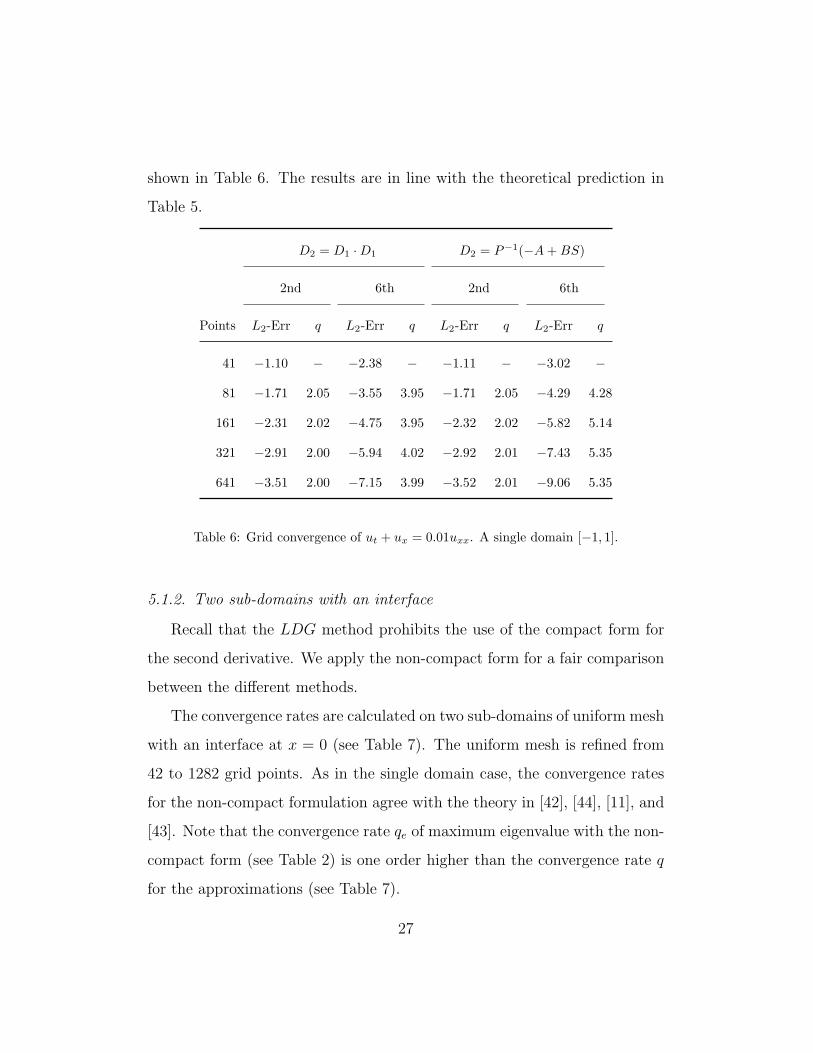
shown in Table 6. The results are in line with the theoretical prediction in
Table 5.
D2 = D1 ·D1 D2 = P−1(−A+BS)
2nd 6th 2nd 6th
Points L2-Err q L2-Err q L2-Err q L2-Err q
41 −1.10 − −2.38 − −1.11 − −3.02 −
81 −1.71 2.05 −3.55 3.95 −1.71 2.05 −4.29 4.28
161 −2.31 2.02 −4.75 3.95 −2.32 2.02 −5.82 5.14
321 −2.91 2.00 −5.94 4.02 −2.92 2.01 −7.43 5.35
641 −3.51 2.00 −7.15 3.99 −3.52 2.01 −9.06 5.35
Table 6: Grid convergence of ut + ux = 0.01uxx. A single domain [−1, 1].
5.1.2. Two sub-domains with an interface
Recall that the LDG method prohibits the use of the compact form for
the second derivative. We apply the non-compact form for a fair comparison
between the different methods.
The convergence rates are calculated on two sub-domains of uniform mesh
with an interface at x = 0 (see Table 7). The uniform mesh is refined from
42 to 1282 grid points. As in the single domain case, the convergence rates
for the non-compact formulation agree with the theory in [42], [44], [11], and
[43]. Note that the convergence rate qe of maximum eigenvalue with the non-
compact form (see Table 2) is one order higher than the convergence rate q
for the approximations (see Table 7).
27

(a) second order accuracy
BON CNGN LDG
Points L2-Err q L2-Err q L2-Err q
41 −1.07 − −1.07 − −1.07 −
81 −1.69 2.13 −1.69 2.13 −1.70 2.14
161 −2.30 2.06 −2.30 2.06 −2.30 2.06
321 −2.90 2.02 −2.90 2.03 −2.91 2.03
641 −3.51 2.01 −3.51 2.01 −3.51 2.01
(b) sixth order accuracy
BON CNGN LDG
Points L2-Err q L2-Err q L2-Err q
41 −2.02 − −2.02 − −1.93 −
81 −3.26 4.25 −3.28 4.40 −3.24 4.49
161 −4.55 4.37 −4.57 4.35 −4.62 4.67
321 −5.79 4.15 −5.80 4.09 −5.93 4.39
641 −7.00 4.00 −7.00 4.00 −7.17 4.14
Table 7: Grid convergence of ut + ux = 0.01uxx. Two sub-domains, uniform mesh in
[−1, 1].
28

Now the convergence rate q is tested on two sub-domains with non-
uniform grid. We start with 41 grid points in the left subdomain and 11
grid points in the right subdomain. For each refinement the grid points
are doubled in both sub-domains. Table 8 presents the results using a non-
compact second derivative. The convergence rate exactly coincide with the
theoretical values.
(a) second order accuracy
BON CNGN LDG
Points L2-Err q L2-Err q L2-Err q
41 + 11 −0.99 − −0.93 − −0.96 −
81 + 21 −1.64 2.19 −1.63 2.29 −1.60 2.14
161 + 41 −2.26 2.12 −2.27 2.13 −2.22 2.05
321 + 81 −2.88 2.05 −2.89 2.03 −2.83 2.01
641 + 161 −3.48 2.01 −3.48 2.01 −3.43 2.00
(b) sixth order accuracy
BON CNGN LDG
Points L2-Err q L2-Err q L2-Err q
41 + 11 −1.45 − −1.34 − −1.33 −
81 + 21 −2.62 3.97 −2.65 4.37 −2.18 2.83
161 + 41 −3.81 4.04 −3.86 4.03 −3.27 3.62
321 + 81 −5.05 4.13 −5.06 3.97 −4.47 3.98
641 + 161 −6.26 4.04 −6.26 3.99 −5.68 4.03
Table 8: Grid convergence for non-compact form. Two sub-domains, non-uniform mesh.
So far we have used the non-compact form. Table 9 shows the conver-
29

gence q for the BON and CNGN schemes on compact form. In Table 9 the
convergence rate for the second and sixth order accurate schemes are in line
with the theoretical conclusion in Table 5. Note that the convergence rates
using the sixth order scheme in Table 9 attain almost 6 while the theoretical
value is 5.
2nd (BOC) 6th (BOC) 2nd (CNGC) 6th (CNGC)
Points L2-Err q L2-Err q L2-Err q L2-Err q
41 −1.07 − −2.35 − −1.07 − −2.37 −
81 −1.68 2.02 −3.77 4.89 −1.69 2.12 −3.79 4.89
161 −2.29 2.02 −5.34 5.30 −2.29 2.01 −5.35 5.28
321 −2.89 2.00 −7.04 5.70 −2.89 2.00 −7.04 5.69
641 −3.50 2.00 −8.83 5.70 −3.49 2.01 −8.82 5.95
Table 9: Grid convergence for compact form. Two sub-domains, non-uniform mesh.
5.1.3. The reflecting properties
To test the reflecting and oscillation properties of these schemes, a “wave”
like analytic solution of (1) is chosen
u = κ exp(−θ(x− ct+ b)2). (31)
The initial data, boundary data and forcing function are modified to adapt
to the analytic solution (31). The forcing function in (1) becomes
F = −ε(− 2κθ + 4κθ2(x− ct+ b)2
)exp
(− θ(x− ct+ b)2
)(32)
In all tests we use a = 1, ε = 0.01, κ = 0.5, θ = 100, b = 0.8 and c = 1.
The exact solutions at T = 0.3, T = 0.8 and T = 1.3 are shown in Figure
30

2. With increasing time, the solution propagate from left to right without
changing form. The calculation in this section is done on an equidistant grid
for both domains.
1 0.5 0 0.5 10
0.05
0.1
0.15
0.2
0.25
0.3
0.35
0.4
0.45
0.5
t=0.3t=0.8t=1.3
Figure 2: Exact solution.
The error of the schemes are presented at T = 0.3, T = 0.8 and T = 1.3
in Figures 3 and 4. We notice that for the SIN scheme (without an interface),
the error propagate from left to right. In both the second order accurate cases
(see Figures 3) and the sixth order accurate case (see Figures 4), the error
propagate from left to right via the interface at x = 0 without reflection for all
compact schemes. However the schemes BON, CNGN and LDG (with non-
compact form) lead to an oscillatory error caused by the interface. The error
attains a maximum when the “wave” pass the interface around T = 0.8 (see
Figures 4). But it is also clearly seen propagating backwards at T = 0.8. The
schemes BOC and CNGC (with compact form) also introduces an oscillation
at interface, however the magnitude of the error is very small compared with
the non-compact schemes.
Sixth order accurate dissipation operators [45] are introduced in the non-
compact schemes BON, CNGN and LDG. The calculations are shown in
31

1 0.8 0.6 0.4 0.2 0 0.2 0.4 0.6 0.8 10.05
0.04
0.03
0.02
0.01
0
0.01
0.02
0.03
0.04
0.05
Error
t=0.3t=0.8t=1.3
(a) SIN
1 0.8 0.6 0.4 0.2 0 0.2 0.4 0.6 0.8 10.05
0.04
0.03
0.02
0.01
0
0.01
0.02
0.03
0.04
0.05
Error
t=0.3t=0.8t=1.3
(b) LDG
1 0.8 0.6 0.4 0.2 0 0.2 0.4 0.6 0.8 10.05
0.04
0.03
0.02
0.01
0
0.01
0.02
0.03
0.04
0.05
Error
t=0.3t=0.8t=1.3
(c) BON
1 0.8 0.6 0.4 0.2 0 0.2 0.4 0.6 0.8 10.05
0.04
0.03
0.02
0.01
0
0.01
0.02
0.03
0.04
0.05Error
t=0.3t=0.8t=1.3
(d) CNGN
1 0.8 0.6 0.4 0.2 0 0.2 0.4 0.6 0.8 10.05
0.04
0.03
0.02
0.01
0
0.01
0.02
0.03
0.04
0.05
Error
t=0.3t=0.8t=1.3
(e) BOC
1 0.8 0.6 0.4 0.2 0 0.2 0.4 0.6 0.8 10.05
0.04
0.03
0.02
0.01
0
0.01
0.02
0.03
0.04
0.05
Error
t=0.3t=0.8t=1.3
(f) CNGC
Figure 3: Error. Second order accuracy. 81 points used. σL2 = −ε/2.
32

1 0.8 0.6 0.4 0.2 0 0.2 0.4 0.6 0.8 10.012
0.009
0.006
0.003
0
0.003
0.006
0.009
0.012
Error
t=0.3t=0.8t=1.3
(a) SIN
1 0.8 0.6 0.4 0.2 0 0.2 0.4 0.6 0.8 10.012
0.009
0.006
0.003
0
0.003
0.006
0.009
0.012
Error
t=0.3t=0.8t=1.3
(b) LDG
1 0.8 0.6 0.4 0.2 0 0.2 0.4 0.6 0.8 10.012
0.009
0.006
0.003
0
0.003
0.006
0.009
0.012
Error
t=0.3t=0.8t=1.3
(c) BON
1 0.8 0.6 0.4 0.2 0 0.2 0.4 0.6 0.8 10.012
0.009
0.006
0.003
0
0.003
0.006
0.009
0.012Error
t=0.3t=0.8t=1.3
(d) CNGN
1 0.8 0.6 0.4 0.2 0 0.2 0.4 0.6 0.8 10.012
0.009
0.006
0.003
0
0.003
0.006
0.009
0.012
Error
t=0.3t=0.8t=1.3
(e) BOC
1 0.8 0.6 0.4 0.2 0 0.2 0.4 0.6 0.8 10.012
0.009
0.006
0.003
0
0.003
0.006
0.009
0.012
Error
t=0.3t=0.8t=1.3
(f) CNGC
Figure 4: Error. Sixth order accuracy. 81 points used. σL2 = −ε/2.
33

Figure 5. By comparing with the calculations in Figure 4 we find that the
artificial dissipation operators kill the non-physical numerical oscillations ef-
ficiently for schemes BON and CNGN. However the artificial dissipation only
reduce the magnitude of the oscillation of LDG to 30%.
1 0.8 0.6 0.4 0.2 0 0.2 0.4 0.6 0.8 10.012
0.009
0.006
0.003
0
0.003
0.006
0.009
0.012
Error
t=0.3t=0.8t=1.3
(a) LDG
1 0.8 0.6 0.4 0.2 0 0.2 0.4 0.6 0.8 10.012
0.009
0.006
0.003
0
0.003
0.006
0.009
0.012
Error
t=0.3t=0.8t=1.3
(b) BON
1 0.8 0.6 0.4 0.2 0 0.2 0.4 0.6 0.8 10.012
0.009
0.006
0.003
0
0.003
0.006
0.009
0.012
Error
t=0.3t=0.8t=1.3
(c) CNGN
Figure 5: Error. Sixth order accuracy, artificial dissipation. 81 points used. σL2 = −ε/2.
5.2. Multi-domains in two-dimensions
The SAT formulation can easily be generalized to several space dimen-
sions. We demonstrate that by using the Baumann-Orden scheme described
34
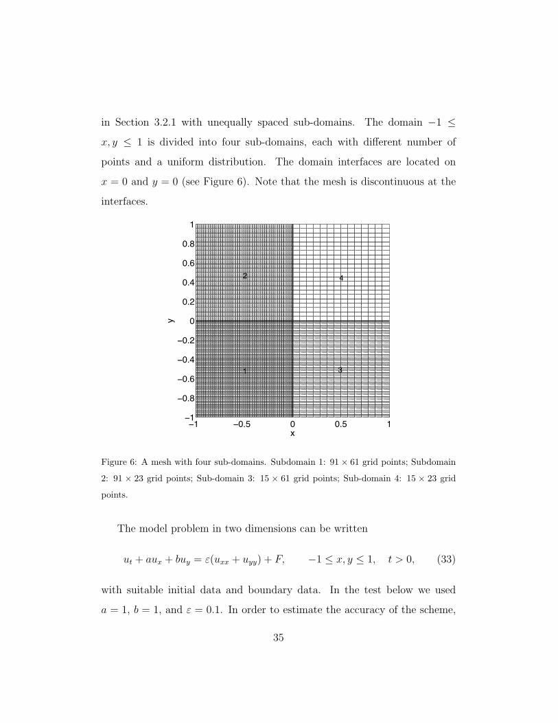
in Section 3.2.1 with unequally spaced sub-domains. The domain −1 ≤
x, y ≤ 1 is divided into four sub-domains, each with different number of
points and a uniform distribution. The domain interfaces are located on
x = 0 and y = 0 (see Figure 6). Note that the mesh is discontinuous at the
interfaces.
1 0.5 0 0.5 11
0.8
0.6
0.4
0.2
0
0.2
0.4
0.6
0.8
1
x
y
1 3
4 2
Figure 6: A mesh with four sub-domains. Subdomain 1: 91× 61 grid points; Subdomain
2: 91 × 23 grid points; Sub-domain 3: 15 × 61 grid points; Sub-domain 4: 15 × 23 grid
points.
The model problem in two dimensions can be written
ut + aux + buy = ε(uxx + uyy) + F, −1 ≤ x, y ≤ 1, t > 0, (33)
with suitable initial data and boundary data. In the test below we used
a = 1, b = 1, and ε = 0.1. In order to estimate the accuracy of the scheme,
35

an exact solution u = sin(2π(x+ y − 2t)) has been chosen. The initial data,
boundary data and the forcing function F are adjusted to correspond to
the exact solution. Table 10 shows a grid-refinement study for three different
orders of accuracy. Note that the convergence rate approaches the theoretical
rates studied previously in the one-dimensional cases.
2nd 4th 6th
Points L2-Err q L2-Err q L2-Err q
4144 −1.57 − −2.17 − −2.08 −
8904 −1.94 2.20 −2.63 2.77 −2.58 3.07
15904 −2.23 2.30 −3.00 2.93 −3.03 3.57
24603 −2.43 2.04 −3.28 2.92 −3.38 3.73
35404 −2.58 2.02 −3.51 2.94 −3.67 3.70
62604 −2.84 2.03 −3.88 2.97 −4.14 3.78
97304 −2.84 2.03 −4.17 3.00 −4.57 3.85
Table 10: The convergence rate of ut + ux + uy = 0.1(uxx + uyy) + F with non-compact
form in four subdomains of nonuniform mesh in two dimensions.
We also consider the reflexion properties from the interfaces in two di-
mensions. The analytic solution
u(x, y, t) = κ exp(−θ((x− c1t+ b1)2 + (y − c2t+ b2)
2)), (34)
is used as boundary and initial data.
In this test, κ = 0.5, θ = 50, c1 = 1, b1 = 0.5, c2 = 1, and c2 = 0.5.
Figure 7 shows the numerical results at t = 0.1, 0.3, 0.5, 0.7, 0.9,
36

and 1.5 with the scheme. Between t = 0.3 and t = 0.7 the vortex propagates
close to the interfaces y = 0 and x = 0. No problems could be detected at
the interfaces and the reflexion is very small indeed, see Figure 8. For even
more complex geometries, we can use our technique with hybrid methods,
see [14], [24] and [46] or the recently developed method with non-matching
grid lines [47].
6. Conclusions
Stable and accurate interface treatments for the linear advection-diffusion
equation have been studied. The treatment is based on SBP operators and
the SAT technique, which lead to an energy estimate and stability. Accurate
high order calculations are performed in both single domain and multiple
domains with an interface.
Three stable interface procedures: the Baumann-Oden method, the Carpenter-
Nordstrom-Gottlieb method and the local discontinuous Galerkin method
have been investigated. The compact form and non-compact form of the
second derivative SBP operators have also been compared.
The spectral radius for the schemes depend on the chosen coefficients. The
interface procedures do not increase the spectral radius if suitable penalty
parameters chosen. In particular, when the centered fluxes were used in the
LDG, the minimal spectral radius was been obtained.
By using the compact form we can obtain one order higher accuracy
than for the non-compact form. Moreover, the compact form introduces less
reflection and oscillation than the non-compact form. Artificial dissipation
can reduce the non-physical oscillation from the interface for the non-compact
37

1 0.5 0 0.5 11
0.8
0.6
0.4
0.2
0
0.2
0.4
0.6
0.8
1
x
y
(a) t = 0.1
1 0.5 0 0.5 11
0.8
0.6
0.4
0.2
0
0.2
0.4
0.6
0.8
1
x
y(b) t = 0.3
1 0.5 0 0.5 11
0.8
0.6
0.4
0.2
0
0.2
0.4
0.6
0.8
1
x
y
(c) t = 0.5
1 0.5 0 0.5 11
0.8
0.6
0.4
0.2
0
0.2
0.4
0.6
0.8
1
x
y
(d) t = 0.7
1 0.5 0 0.5 11
0.8
0.6
0.4
0.2
0
0.2
0.4
0.6
0.8
1
x
y
(e) t = 0.9
1 0.5 0 0.5 11
0.8
0.6
0.4
0.2
0
0.2
0.4
0.6
0.8
1
x
y
(f) t = 1.5
Figure 7: The calculation on a mesh with four subdomains and sixth order accuracy.
Subdomain 1: 81× 61 points; subdomain 2: 81× 41 points; subdomain 3: 31× 61 points;
subdomain 4: 31× 41 points.
38

1 0.5 0 0.5 15
2.5
0
2.5
5 x 10 3
x (y=0)
Erro
r
t=0.3t=0.5t=0.7
(a) interface y = 0
1 0.5 0 0.5 15
2.5
0
2.5
5 x 10 3
y (x=0)
Erro
r
t=0.3t=0.5t=0.7
(b) interface x = 0
Figure 8: The error on the interfaces y = 0 and x = 0.
form.
In short, this analysis show that only minor differences separates the
different interface procedures. However the local discontinuous Galerkin
method is more difficult to implement since the scheme requires one to rewrite
the original viscous problem as a first order system of equations.
Appendix
Here we prove Lemma 4.1.
When s ≤ −a2/(4ε), s ∈ <, the term√
1 + 4sε/a2 is a pure imaginary
number and κ1,2 becomes
κ1,2 =a
2ε
(1±
√1 +
4sε
a2
)= c(1± b(s)i)
where c = a/(2ε) > 0 ∈ < is a constant and b(s) =∣∣√−(1 + 4sε/a2)
∣∣ ≥ 0 ∈
39

<. Substituting κ1,2 into (27) yields
detC(s) =[1 + βc(1− b(s)i)
]c(1 + b(s)i)ec(1+b(s)i)
−[1 + βc(1 + b(s)i)
]c(1− b(s)i)ec(1−b(s)i)
= 2cec[b(s) cos(cb(s)) + (1 + βc+ βcb2(s)) sin(cb(s))
]i
= F (b(s))i
(35)
which only contains imaginary parts and the continuous real-function
F (b(s)) = 2cec[b(s) cos(cb(s))+(1+βc+βcb2(s)) sin(cb(s))
], F (b(s)) ∈ <.
We have
F(b(s) =
2nπ
c
)= 2cec
2nπ
c= 4necπ > 0,
F(b(s) =
(2n+ 1)π
c
)= −2cec
2nπ
c= −4necπ < 0. n = 1, 2, . . .
(36)
As a result, there exists b(s) ∈ [2nπ/c, (2n+ 1)π/c] or
s = −a2(b2 + 1)
4ε∈[−a
2((2n+ 1)π)2 + c2)
4εc2,−a
2(2nπ)2 + c2)
4εc2
], n = 1, 2, . . . ,
such that F (b(s)) = 0. Therefore, (27) has a solution for s ≤ −a2/(4ε),
s ∈ <.
However, we note that when s > −a2/(4ε), s ∈ <, the equation (27) has
no solution. To verify this, we rewrite the term κ1,2,
κ1,2 =a
2ε
(1±
√1 +
4sε
a2
)= c(1± b(s))
where b(s) = |√
1 + 4sε/a2| > 0, b(s) ∈ <.
Applying κ1,2 to (27) leads to
detC(s) =[1 + βc(1− b(s))
]c(1 + b(s))ec(1+b(s))
−[1 + βc(1 + b(s))
]c(1− b(s))ec(1−b(s))
= cec(1−b(s))[e2cb(s)(1 + b(s) + βc− βcb2(s))− (1− b(s) + βc− βcb2(s))
]40
The inequality derived from the well-posedness condition (3),
−1 ≤ βc ≤ 0,
implies that the term 1 + b(s) + βc − βcb2(s) is positive. Consequently we
have
detC(s) >cec(1−b(s))[(1 + b(s) + βc− βcb2(s))− (1− b(s) + βc− βcb2(s))
]=2cec(1−b(s))b(s) > 0
(37)
Therefore, detC(s) is always positive for s > −a2/(4ε), s ∈ <. �
References
[1] M. Darbandi and A. Naderi. Multiblock hybrid grid finite volume
method to solve flow in irregular geometries. Computer Methods in
Applied Mechanics and Engineering, 196:321–336, 2006.
[2] A. Rizzi, P. Eliasson, I. Lindblad, C. Hirsch, C. Lacour, and J. Hauser.
The engineering of multiblock multi-grid software for Navier-Stokes flows
on structured meshes. Computers and Fluids, 22:341–367, 1993.
[3] E. van der Weide, G. Kalitzin, J. Schluter, and J.J. Alonso. Unsteady
turbomachinery computations using massively parallel platforms. AIAA
Paper 2006-421, 2006.
[4] J. Chao, A. Haselbacher, and S. Balachandar. A massively parallel multi-
block hybrid compact-WENO scheme for compressible flows. Journal of
Computational Physics, 228(19):7473–7491, Oct 20 2009.
41

[5] A Rouboa and E Monteiro. Heat transfer in multi-block grid during so-
lidification: Performance of finite differences and finite volume methods.
Journal of Materials Processing Technology, 204(1-3):451–458, Aug 11
2008.
[6] L Lehner, O Reula, and M Tiglio. Multi-block simulations in general rel-
ativity: high-order discretizations, numerical stability and applications.
Classical and Quantum Gravity, 22(24):5283–5321, Dec 21 2005.
[7] XG Zhang, GA Blaisdell, and AS Lyrintzis. High-order compact schemes
with filters on multi-block domains. Jornal of Scientific Computing,
21(3):321–339, Dec 2004.
[8] M.H. Carpenter, J. Nordstrom, and D. Gottlieb. A stable and con-
servative interface treatment of arbitrary spatial accuracy. Journal of
Computational Physics, 148:341–365, 1999.
[9] H.-O. Kreiss and G. Scherer. Finite element and finite difference meth-
ods for hyperbolic partial differential equations, in: C. De Boor (Ed.),
Mathematical Aspects of Finite Elements in Partial Differential Equa-
tion. Academic Press, New York, 1974.
[10] K. Mattsson. Boundary procedures for summation-by-parts operators.
Journal of Scientific Computing, 18(1):133–153, 2003.
[11] K. Mattsson and J. Nordstrom. Summation by parts operators for finite
difference approximations of second derivatives. Journal of Computa-
tional Physics, 199:503–540, 2004.
42

[12] J. Nordstrom and M. H. Carpenter. High-order finite difference methods,
multidimensional linear problems and curvilinear coordinates. Journal
of Computational Physics, 173:149–174, 2001.
[13] J. Nordstrom and R. Gustafsson. High order finite difference approxi-
mations of electromagnetic wave propagation close to material disconti-
nuities. Journal of Scientific Computing, 18(2):215–234, 2003.
[14] J. Nordstrom and J. Gong. A stable hybrid method for hyperbolic
problems. Journal of Computational Physics, 212:436–453, 2006.
[15] B. Strand. Summation by parts for finite difference approximation for
d/dx. Journal of Computational Physic, 110(1):47–67, 1994.
[16] M.H. Carpenter, D. Gottlieb, and S. Abarbanel. Time-stable bound-
ary conditions for finite-difference schemes solving hyperbolic systems:
Methodology and application to high-order compact schemes. Journal
of Computational Physics, 111(2):220–236, 1994.
[17] J. Nordstrom, K. Forsberg, C. Adamsson, and P. Eliasson. Finite volume
methods, unstructured meshes and strict stability. Applied Numerical
Mathematics, 45:453–473, 2003.
[18] B. Strand. Numerical studies of hyperbolic IBVP with high-order fi-
nite difference operators satisfying a summation by parts rule. Applied
Numerical Mathematics, 26(4):497–521, 1998.
[19] M. Svard, M.H. Carpenter, and J. Nordstrom. A stable high-order finite
difference scheme for the compressible Navier-Stokes equations: far-field
43

boundary conditions. Journal of Computational Physics, 225(1):1020–
1038, 2007.
[20] M. Svard and J. Nordstrom. A stable high-order finite difference scheme
for the compressible Navier-Stokes equations: wall boundary conditions.
Journal of Computational Physics, 227:4805–4824, 2008.
[21] J. Nordstrom, J. Gong, E. van der Weide, and M. Svard. A stable
and conservative high order multi-block method for the compressible
Navier-Stokes equations. Journal of Computational Physics, 228:9020–
9035, 2009.
[22] K. Mattsson, M. Svard, M.H. Carpenter, and J. Nordstrom. High-order
accurate computations for unsteady aerodynamics. Computers & Fluids,
36(3):636–649, Mar 2007.
[23] M. H. Carpenter, J. Nordstrom, and D. Gottlieb. Revisiting and extend-
ing interface penalties for multi-domain summation-by-parts operators.
Journal of Scientific Computing, 45:118–150, 2010.
[24] J. Nordstrom and J. Gong. A stable and efficient hybrid method
for aeroacoustic sound generation and propagation. Comptes Rendus
Mecanique, 333:713–718, 2005.
[25] F. Edelvik and G. Ledfelt. A comparsion of time domain hybrid solvers
for complex scattering problems. Internation Journal of Numerical Mod-
eling, 15(5-6):475–487, 2002.
[26] F. Edelvik and G. Ledfelt. Explicit hybrid time domain solver for the
44

Maxwell’s equations in 3d. Journal of Scientific Computing, 15(1):61–
78, 2000.
[27] T. Rylander and A. Bondeson. Stable FEM-FDTD hybrid method for
Maxwell’s equations. Computational Physics Communication, 125:75–
82, 2000.
[28] M. Djordjevicand and B. M. Notaros. Higher order hybrid method of
moments-physical optics modelling technique for radiation and scatter-
ing from large perfectly conduction surfaces. IEEE Transactions on
Antennas and Propagation, 53(2):800–813, 2005.
[29] A. Burbeau and P. Sagaut. A dynamic p-adaptive discontinuous
Galerkin method for viscous flow with shcoks. Computers and Fluids,
34(4-5):401–417, 2005.
[30] X. Ferrieres, J.P. Parmantier, S. Bertuol, and A.R. Ruddle. Application
of a hybrid finite difference/finite volume method to solve an automo-
tive emc problem. IEEE Transactions on Electromagnetic Compatibility,
46(4):624–634, 2004.
[31] A. Monorchio, A.R. Bretones, R. Mittra, G. Manara, and R.G. Martin.
A hybrid time-domain technique that combines the finite element, finite
difference and method of moment techniques to solve complex electro-
magnetic problem. IEEE Transactions on Antennas and Propagation,
52(10):2666–2674, 2004.
[32] B. Gustafsson, H.-O. Kreiss, and J. Oliger. Time Dependent Problems
and Difference Methods. John Wiley & Sons, Inc., 1995.
45

[33] J. Lindstrom and J. Nordstrom. A stable and high-order accurate
conjugate heat transfer problem. Journal of Ccomputational Physics,
229(14):5440–5456, Jul 20 2010.
[34] J. Nordstrom and S. Eriksson. Fluid Structure Interaction Problems:
the Necessity of a Well Posed, Stable and Accurate Formulation. Com-
munications in Computational Physics, 8(5):1111–1138, Nov 2010.
[35] S. Eriksson, Q. Abbas, and J. Nordstrom. A stable and conservative
method for locally adapting the design order of finite difference schemes.
Journal of Computational Physics, 230(11, Sp. Iss. SI):4216–4231, May
20 2011.
[36] C.E. Baumann and J.T. Oden. A discontinuous hp finite element method
for convection-diffusion problems. Computer Methods in Applied Me-
chanics and Engineering, 175:331–341, 1999.
[37] W.H. Reed and T. R. Hill. Triangular mesh methods for the neutron
transport equation. Technical Report LA-UR-73-479, Los Alamos Sci-
entific Laboratory, 1973.
[38] B. Cockburn and C.-W. Shu. The local discontinuous Galerkin method
for time-dependent convection-diffusion systems. SIAM Journal of Nu-
merical Analysis, 35:2440–2463, 1998.
[39] C.-W. Shu. Different formulations of the discontinuous Galerkin method
for the viscous terms. In Z.-C. Shi, M. Mu, W. Xue, and J. Zou, editors,
Advances in Scientific Computing. Science Press, 2001.
46

[40] J Nordstrom. The Influence of Open Boundary Cconditions on the
Convergence to Steady-State for the Navier-Stokes Equations. Journal
of Computational Physics, 85(1):210–244, Nov 1989.
[41] M. Svard, K. Mattsson, and J. Nordstrom. Steady-stable computations
using summation-by-parts operators. Journal of Scientific Computing,
24(1):79–95, 2005.
[42] B. Gustafsson. The convergence rate for difference approximation to
mixed initial boundary value problems. Mathematics of Computation,
29, 1975.
[43] M. Svard and J. Nordstrom. On the order of accuracy for difference
approximations of initial-boundary value problems. Journal of Compu-
tational Physics, 218(1):333–352, 2006.
[44] B. Gustafsson. The convergence rate for difference approximation to
general mixed initial boundary value problems. SIAM Journal on Nu-
merical Analysis, 18(2):179–190, 1981.
[45] K. Mattsson, M. Svard, and J. Nordstrom. Stable and accurate artificial
dissipation. Journal of Scientific Computing, 21(1):57–79, 2004.
[46] J. Gong and J. Nordstrom. A stable and efficient hybrid method for
viscous problems in complex geometries. Journal of Computational
Physics, 226:1291–1309, 2006.
[47] K. Mattsson and M. H. Carpenter. Stable and accurate interpolation
operators for high-order multi-block finite-difference methods. SIAM
Journal on Scientific Computing, 32(4):2298–2320, 2010.
47