intergenerational social mobility in european oecd countries

Unclassified ECO/WKP(2009)50 Organisation de Coopération et de Développement Économiques Organisation for Economic Co-operation and Development 07-Jul-2009 ___________________________________________________________________________________________

English - Or. English ECONOMICS DEPARTMENT

INTERGENERATIONAL SOCIAL MOBILITY IN EUROPEAN OECD COUNTRIES ECONOMICS DEPARTMENT WORKING PAPERS NO.709

By Orsetta Causa, Sophie Dantan and Åsa Johansson

All Economics Department Working Papers are available through OECD's internet web site at www.oecd.org/eco/working_papers

JT03267758

Document complet disponible sur OLIS dans son format d'origine Complete document available on OLIS in its original format

EC

O/W

KP(2009)50

Unclassified

English - O

r. English

ECO/WKP(2009)50

2

ABSTRACT/RESUMÉ

Intergenerational social mobility in European OECD countries

This paper breaks new ground by providing comparable estimates of intergenerational wage and education persistence across 14 European OECD countries based on a new micro data from Eurostat. A further novelty is that it examines the potential role of public policies and labour and product market institutions in explaining observed differences in intergenerational wage mobility across countries. The empirical estimates show that intergenerational wage persistence is relatively high in southern European countries, as well as in the United Kingdom. Likewise, intergenerational persistence in education is relatively high both in southern European countries and in Luxembourg and Ireland. By contrast, both persistence in wages and education tends to be lower in Nordic countries. In addition, empirical results show that education is one important driver of intergenerational wage persistence across European countries. There is a positive cross-country correlation between intergenerational wage mobility and redistributive policies, as well as a positive correlation between wage-setting institutions that compress the wage distribution and mobility.

JEL classification: J60; J62; C20; C21; I20; H23; H31

Keywords: intergenerational wage mobility; intergenerational education mobility; education; public policies; household survey data

********

Mobilité sociale intergénérationnelle dans les pays européenne de l'OCDE

Cet article comble une faille dans la littérature en présentant de nouvelles mesures harmonisées du degré de mobilité sociale intergénérationnelle de salaire et d’éducation pour 15 pays Européens de l’OCDE, grâce à l’utilisation de nouvelles donnes microéconomiques publiées par Eurostat. Il analyse également le rôle des politiques en vigueur sur le marché du travail et sur le marché des produits dans l’explication des différences de mobilité entre pays. Les estimations suggèrent que la persistance intergénérationnelle des salaires est relativement élevée dans les pays du Sud de l’Europe, ainsi qu’au Royaume-Uni. De la même façon, la persistance intergénérationnelle du niveau d’éducation est relativement élevée dans les pays du Sud de l’Europe, ainsi qu’au Luxembourg. En revanche, la persistance intergénérationnelle, aussi bien du niveau de l’éducation que des salaires, est relativement faible dans les pays Nordiques. De plus, les résultats empiriques montrent que dans les pays Européens de l’OCDE, l’éducation est un vecteur important de la mobilité sociale intergénérationnelle. L’étude suggère qu’il existe une corrélation positive entre la mobilité sociale intergénérationnelle des salaires et la générosité des politiques de redistribution du revenu, résultat qui s’applique également à l’analyse de l’impact des instances de négociation collective qui compressent la grille salariale.

Classification JEL: J60; J62; C20; C21; I20; H23; H31

Mots clés : mobilité sociale intergénérationnelle dans les salaries ; mobilité sociale intergénérationnelle dans l’éducation ; éducation ; politiques publiques ; données de ménages

ECO/WKP(2009)50

3

Copyright OECD, 2009

Application for permission to reproduce or translate all, or part of, this material should be made to: Head of Publications Service, OECD, 2 rue André-Pascal, 75775 Paris CEDEX 16, France.

ECO/WKP(2009)50

4

TABLE OF CONTENTS

INTERGENERATIONAL SOCIAL MOBILITY IN EUROPEAN OECD COUNTRIES ........................... 5

Introduction ................................................................................................................................................. 5 Related literature and contributions of this paper ........................................................................................ 6 Analytical and estimation framework ......................................................................................................... 8

Wage persistence and the role of education ............................................................................................. 8 Data and measurement issues ................................................................................................................ 10

Patterns of intergenerational social mobility in European OECD countries ............................................. 11 Intergenerational wage persistence across European OECD countries ................................................. 11 Intergenerational education persistence across European OECD countries .......................................... 17

Public policies and intergenerational persistence in wages ....................................................................... 20 Identifying the role of policies ............................................................................................................... 20 Cross-country and cross-cohort estimates ............................................................................................. 22

Concluding remarks .................................................................................................................................. 25 APPENDIX: DATA SOURCES FOR POLICY AND INSTITUTIONAL VARIABLES ....................... 26 GLOSSARY .............................................................................................................................................. 28

BIBLIOGRAPHY ......................................................................................................................................... 30

Tables

1. The EU-SILC sample: descriptive statistics .......................................................................................... 34 2. The influence of father's educational attainment on son's wage ............................................................ 35 3. The influence of father's educational attainment on a daughter's wage ................................................ 38 4. Persistence in wages is higher at the top and the bottom ...................................................................... 41 5. Long-distance mobility: probability to move from the bottom to the top and vice versa ..................... 42 6. The influence of parental background on individuals' adult wages: quantile regressions ..................... 43 7. Baseline cross-country results, men and women ................................................................................... 45 8. The influence of policies on intergenerational wage persistence, men ................................................. 46 9. The influence of policies on intergenerational wage persistence, women ............................................ 47

Figures

1. Wage premium and penalty due to family background: selected European OECD countries .............. 48 2. Wage premium and penalty due to parental background, controlling for own education: selected European OECD countries ........................................................................................................................ 49 3. Summary measure of wage persistence: selected European OECD countries ...................................... 50 4. The risk ratio of achieving higher education: selected European OECD countries .............................. 51 5. Probability premium and penalty of achieving tertiary education: selected European OECD countries52 6. Probability premium and penalty of achieving below-secondary education: selected European OECD countries .................................................................................................................................................... 53 7. Summary measures of persistence in education: selected European OECD countries ......................... 54

ECO/WKP(2009)50

5

INTERGENERATIONAL SOCIAL MOBILITY IN EUROPEAN OECD COUNTRIES

By Orsetta Causa, Sophie Dantan and Åsa Johansson1

Introduction

1. This paper assesses patterns in intergenerational social mobility across European OECD countries and examines the potential role of policies in explaining observed differences across countries. Intergenerational social mobility refers to the relationship between the socio-economic status of parents and that of their offspring when they become adults. In both cases, status can be measured in several ways: by income, wage, social class, education or occupation. As in most other economic research in this area, this study focuses on wages and education.2 More precisely, the focus is on the impact of a father’s education on both his offspring’s education and wages. For brevity, the remainder of this paper will refer to the impact of a father’s education on offspring’s wages as “wage mobility” or “wage persistence”.3 It provides three contributions. First, it assesses the degree of intergenerational wage and education persistence across European OECD countries in a comparative perspective. Second, it analyses the role of education as a determinant of intergenerational wage persistence across countries. Third, it investigates the role of public policies and institutions, particularly those having an influence on cross-sectional income inequality, in mitigating or reinforcing wage persistence across generations.

2. A number of seemingly robust conclusions emerge from the analysis:

• Across European OECD countries covered by the analysis there is a substantial wage premium associated with growing up in a higher-educated family, whereas there is a penalty with growing up in a lower-educated family, even after controlling for a number of individual characteristics. The premium and penalty are particularly large in southern European countries, as well as in the

1. Corresponding authors are: Orsetta Causa ([email protected]), Åsa Johansson

([email protected]) both at the OECD Economics Department and Sophie Dantan ([email protected]) at Université Cergy-Pontoise. The authors would like to thank Anna d’Addio, Jørgen Elmeskov, Stephen Machin, Fabrice Murtin, Giuseppe Nicoletti, and Jean-Luc Schneider for their valuable comments and Chatherine Chapuis for excellent statistical work, as well as Irene Sinha for excellent editorial support. The views expressed in this paper are those of the authors and do not necessarily reflect those of the OECD or its member countries.

2. Economists typically analyse income or wage mobility, while sociologists focus on mobility across “social classes” and occupations (see Erikson and Goldthorpe, 1992 for an overview of social class mobility). One advantage of measuring intergenerational mobility by class or occupation is that data restrictions are much less stringent as retrospective information on parents’ occupation is often available. However, there is an important disadvantage associated with the limited cross-country comparability of occupation and “social classes”.

3 . As explained below, there are good reasons for doing so because a father’s education can be considered to be an appropriate proxy for family income.

ECO/WKP(2009)50

6

United Kingdom. The penalty is also high in Luxembourg and Ireland. In general, wage persistence across generations, measured as the difference between the wage premium and penalty, is slightly stronger for sons than for daughters.

• The degree of persistence in wages across generations differs along the wage distribution. In several countries the wage penalty associated with a having a low-educated father is higher at the top of the wage distribution. To the extent that wage is correlated with ability, this result suggests that more able children of low-educated fathers may face financial constraints in access to tertiary education.

• Similarly, across the countries covered by the analysis, there is substantial persistence in educational achievement across generations. In particular, the probability of achieving tertiary education is higher for offspring of higher-educated families, while, other factors controlled for, it is much smaller for offspring of lower-educated families. The increase in the probability of achieving tertiary education is particularly strong in Luxembourg, Italy, Finland and Denmark where it is 30 percentage points higher for a son whose father had tertiary education compared to one whose father had upper-secondary education.

• There is a positive cross-country correlation between intergenerational wage mobility and redistributive policies.

• Wage-setting institutions that compress the wage distribution are associated with lower intergenerational wage persistence.

• Stricter labour market regulation is associated with higher wage persistence across generations, while stricter product market regulation is associated with lower wage persistence.

3. The remainder of the paper is organised as follows. Section 2 introduces the analytical and estimation framework. Section 3 presents, on a country-by-country basis, measures of wage and educational persistence and assesses the role of education as a determinant of wage persistence. Section 4 investigates the role of policies and institutions in understanding differences in intergenerational wage persistence across European OECD countries. Section 5 concludes.

Related literature and contributions of this paper

4. Economic research estimating the extent of intergenerational income persistence is large and increasing. Most of it is based on the estimation of the so-called "intergenerational income elasticity", which measures the extent to which children’s income levels reflect those of their parents. When this elasticity is equal to zero, there is complete mobility in the sense that parents’ and their offsprings' income are unrelated. By contrast, a value of one represents a situation with complete immobility, where the income condition of parents is fully mirrored in that of their offspring. Usually, these studies tend to find that persistence is relatively high in the United States but lower in the Nordic European countries and Canada (Corak, 2006; d’Addio, 2007).4 While this cross-country pattern is relatively well-established in the literature, although for a relatively small subset of countries, the assessment of the precise level of income persistence within countries is far from being established, mostly because of substantial measurement error in the estimation of the intergenerational income elasticity (e.g. d’Addio, 2007 for an overview).

4. Some caution is needed: it should be borne in mind that this comparison is based on different studies, using

different samples, estimation methods, variable definitions and time periods.

ECO/WKP(2009)50

7

5. In most cases the empirical studies on the intergenerational transmission of income are, in one way or another, related to the well-known Becker-Tomes model (Becker and Tomes, 1979; 1986). In this model, parents sacrifice a share of their consumption possibilities to invest in the human capital of their children. Together with the intergenerational transmission of “endowments” (e.g. genetic and wealth inheritance), these investments generate the observed pattern of persistence in incomes over generations.

6. The role of education in explaining intergenerational persistence in income has been emphasised in recent work (e.g. Bourguignon et al. 2003; Blanden et al. 2006; Blanden et al. 2005 and Blanden 2008a). In order to assess the contribution of education to intergenerational income persistence, as well as to investigate its cross-country distribution, these studies decompose the intergenerational income elasticity into three parts. The first is attributable to differences in educational attainment between individuals from different backgrounds or income groups, the second to differences in the returns to education in the labour market, and the third “unexplained” part is not transmitted through education.

7. Among the few cross-country studies, Solon (2004) uses the Becker-Tomes model to explore why intergenerational income persistence may vary across countries and over time. His analysis emphasises the role of education in generating intergenerational persistence. It shows that the relationship between parental income, children’s related human capital, and the labour market returns from this capital plays a crucial role in the transmission of economic status between generations. More specifically, intergenerational income persistence is found to be greater, the larger the inheritability of income-related traits (such as the propensity to undertake education and work ethics), the more efficient the investments in human capital, and the higher the earnings returns to human capital, while persistence decreases with the progressivity of public investment in human capital.

8. The Solon model also establishes a link between intergenerational income persistence and cross-sectional income inequality. It is possible that a country with greater (post tax and transfers) income inequality might also have greater inequalities in the investments that rich and poor parents can make for their children’s development. Indeed, if income affects access to education, e.g. because of liquidity constraints, the ability to take advantage of the high returns to education will be limited to richer households. At the same time, this effect will depend upon how progressive public policy is, i.e. the degree to which children from less advantaged backgrounds disproportionately benefit from public programmes. Hence, while in the Solon model higher returns to education are associated with higher persistence, it is clear that is not the return per se that matters, but rather the opportunity for children from disadvantaged backgrounds to reap the benefits of education. Against this background, the mechanisms underlying the relationship between intergenerational income mobility and cross-sectional income inequality are broader than those implied by variation in the returns to education; for instance they might include policies and institutions affecting access to education by children from families with different backgrounds.

9. One of the main conjectures of the Solon model is, therefore, that the same policies influencing cross-sectional income inequality also affect intergenerational income persistence. Recent empirical work has provided evidence supporting this prediction. A number of authors found a positive correlation between cross-sectional income inequality and intergenerational income or wage persistence, suggesting that countries with the most equal distribution of income at one point in time also exhibit the highest income mobility across generations (Björklund and Jäntti, 1997; Gottschalk and Smeeding, 1997; Aaberge et al. 2002; Andrews and Leigh, 2007). As mentioned earlier, possible explanations of this relationship include not only differences in the returns to education but also the idea that a number of policies and labour market institutions, such as tax and transfers, wage-setting systems and income replacement rates, are important for understanding both intergenerational mobility and the level of cross-section inequality (e.g. d’Addio, 2007). The influence of these policies and institutions has not yet been investigated empirically, partly due to data, measurement and identification issues.

ECO/WKP(2009)50

8

10. Cross-country comparison of intergenerational social mobility is often hindered by the fact that individual studies are not carried out with an explicit comparative aim as different studies use different samples, variable definitions, and estimation methods. This study seeks to fill this gap by using a new harmonised, microeconomic cross-country dataset. Using these data, comparable and consistent estimates of intergenerational wage and education persistence are estimated for 14 European OECD countries. Moreover, the role of education in driving wage mobility across generations is examined and the influence of policies and institutions on intergenerational wage persistence is investigated in a multivariate framework. Focusing on the influence of cross-sectional inequality, the paper looks at the potential for policies that affect the dispersion of cross-sectional incomes and/or parents' wages to influence wage persistence across generations.

Analytical and estimation framework

Wage persistence and the role of education

11. Consistent with recent research, the empirical analysis in this study attempts to understand the channels through which parental background influences individuals’ wages by decomposing wage persistence into a part which is related to persistence in education and the returns to education, and another which is not. More formally, it is assumed that there are three broad educational attainment levels (high, medium, and low). In each family i the offspring’s wages reflect both the influence of individual effort, measured by the level of educational attainment ECi -- where ECi is a vector (1,0) if attainment is high or a vector (0,1) if attainment is low (medium education being the reference category) -- and the influence of parental background Ei, which is proxied by the highest level of education attained by the offspring’s father (again low or high):

1ln iiiii XcECbEaW εα +⋅+⋅+⋅+= (1)

where ln Wi is the log of the gross hourly wage of adult child i, Xi is a set of other “Mincerian” individual characteristics affecting wages, and ε1i is an error term. In this specification, vector a, where a= (ahigh, alow), measures the direct influence of parental educational background on wages, while vector b, b= ( bhigh, blow), captures the labour market returns of offsprings’ education.

12. In theory, the preferred measure of parental background is some estimate of long-run permanent income, such as household’s disposable income, as this would most directly influence an individual's standard of living (e.g. Chadwick and Solon, 2002; Solon 2004; Lee and Solon, 2006) and would be less volatile than current wages. In practice, accurate measurement of a household’s disposable income is difficult as it should take into account the structure of the household, the extent of female participation in the labour market, as well as the different sources of income (e.g. earnings, assets, welfare). Empirical studies on intergenerational income mobility have highlighted the importance of properly measuring family background, as well as the consequences on mobility estimates associated with various forms of measurement error, most notably that arising from life cycle effects in earnings data (e.g. d’Addio, 2007).

13. The dataset used in this study does not contain any data on parental income or wages. As discussed above, parental background is measured by a father’s education. Indeed, research has generally shown that fathers’ background variables are better predictors of sons' (and daughters’) outcomes than those of mothers (e.g. Nguyen and Getinet, 2003). 5 Also, the level of education can be considered as a 5. Some studies have shown that for daughters the socio-economic status of mothers is more important than

that of fathers (Österberg, 2000). Nevertheless, most results in this study are robust to the use of mothers’ education as a proxy for parental background, which is not surprising given the widespread existence of assortative mating (e.g. Kalmijn, 1994; Epstein and Guttman, 1984).

ECO/WKP(2009)50

9

proxy for permanent income or social status as it is less likely to suffer from transitory measurement errors or life-cycle bias than wages, while being highly correlated with wages in most countries (e.g. Solon, 2002).6

14. It is further assumed that the offsprings’ educational attainment is related to that of a father’s, as follows:

2iiii XgEdjEC ε+⋅+⋅+= (2)

Combining equation (1) and (2) yields,

3ln iiii XhEfeW ε+⋅+⋅⋅+= (3)

where f=a+bd, h=c+bg, e=α+bj and ε3i = bε2i + ε1i.

15. The coefficient f captures the total effect of parental background on individual wages. This effect can be decomposed in a direct effect (a) and an indirect effect through education (bd), which, in turn, consists of the returns to education in the labour market (b) and the strength of the influence of father’s education on his offspring’s education (d). The direct effect can be thought to capture social norms (such as work ethics), social network effects (such as family connections in accessing the labour market), or wealth transfers, while the indirect effect captures the access to education for individuals from different family backgrounds (e.g. Bourguignon et al. 2003). To the extent that individual wages reflect individual productivity, a related interpretation is that equation (1) could be thought as “augmented” productivity equation, where parental background is added to the standard Mincerian determinants of wage. In this framework, parameter d would capture the transmission of productivity across generations, while parameter a would capture individuals’ success in the labour market through the other channels mentioned above (“social stratification”).7

16. To investigate the intergenerational channels identified above, the empirical strategy adopted in this paper proceeds in three steps: i) estimate equation (3), as a measure of the overall influence of parental background on individuals’ wages; ii) estimate equation (1), as a measure of the influence of parental background on individuals’ wages, controlling for individuals’ educational achievement, in order to find out whether parental background has a direct influence, over and above any effect via education; iii) estimate equation (2) as a measure of persistence in education.

17. The impact of parental background on individual outcomes combines the joint impact of “nature” and “nurture” on them. Thus, the estimates of the impact of parental background may also include the transmission of heritable ability. There is ample debate in the literature on the relative importance of these components in accounting for the influence of parental background on individual outcomes. The studies that can provide some guidance on this issue are based on samples of twins or adopted individuals, a very stringent data requirement in the present context (Sacerdote, 2002; Plug and Vijverberg, 2003; 2005). However, there is no reason to believe that genetic inheritability varies systematically across countries.

6. Because the dataset does not contain information on parental wages or incomes, two-stage Instrumental

Variables techniques cannot be implemented. These estimation techniques require the existence of an alternative micro household data set of “pseudo-parents” to be able to predict parents’ wages or incomes (e.g. Björklund and Jäntti, 1997; Lefranc and Trannoy, 2005).

7 . Empirically this interpretation has a somewhat limited interest: individual productivity can arguably be directly impacted by parental background (e.g. through work ethics or attitudes towards risk), over and above the impact of parental background on individual educational attainment.

ECO/WKP(2009)50

10

Therefore, the extent to which inheritability can account for the cross-country variation in the influence of parental background on individual outcomes is limited. Against this background, this paper adopts a comparative approach by analysing to what extent estimates of equations (1) - (3) differ across countries.

Data and measurement issues

18. The empirical analysis relies on the recently released European Union Statistics on Income and Living Conditions (EU-SILC) household database. EU-SILC is the first international micro dataset that allows quantitative analysis of the transmission of both social advantage and disadvantage across countries in a comparable way.8 The analysis focuses on the 2005 EU-SILC cross-section, which includes a specific module on intergenerational transmission of poverty.9 This module allows linking economic and educational outcomes of successive cohorts of individuals to their family’s socio-economic background. Individuals aged between 24 and 64 from a sample of the households covered by the EU-SILC survey are asked retrospective information on their socio-economic situation as teenagers. Such retrospective information covers family composition, age, educational levels, activity status and occupation of parents, as well as an indicator of financial distress conditions.

19. The sample used in the analysis consists of individuals aged 25 to 54 and is divided into three successive age groups or cohorts: 25-34, 35-44 and 45-54 years of age. Most results of the country-by-country analysis are presented for the 35-44 year old cohort in order to reduce life-cycle measurement error in individuals’ economic outcomes (Haider and Solon, 2006). For the same reason, individuals that are selected to respond to the intergenerational module, but are reported to still be in education, are dropped from the analysis. However, including them has no impact on the results. Conversely, the variation across cohorts is used to identify the association between policies and wage persistence in a panel data setting.

20. Individuals’ earnings are measured by gross hourly wages for employees.10 Self employed are excluded from the sample, due to well-known difficulties of properly reporting and measuring their income. The sample is restricted to individuals who declare having worked more than 15 hours per week

8 . The EU-SILC collects timely and harmonised cross-sectional and longitudinal multidimensional micro data

on income, poverty and social exclusion within the European Statistical System (ESS). It was launched in 2004 in 13 member countries, plus Norway and Iceland, and currently covers the years 2004, 2005 and 2006 for up to 27 countries (25 member countries plus Norway and Iceland). This analysis excludes some central and eastern European OECD countries due to their particular situation as transition economies, which could influence intergenerational mobility patterns in those countries. Germany is not included in either because inspection of the dataset revealed a sizeable discrepancy between EU-SILC data on educational attainment by cohort and official statistics of the population’s educational attainment, as reported in the OECD Education at a Glance database, as well as in the German socio-economic panel. While there are a number of reasons to expect discrepancies across different sources, their size in the case of the EU-SILC database was considered to be too high for it to be reliable enough for statistical inference purposes.

9. Exploiting the longitudinal dimension of the data would require a longer time span than is currently available in the EU-SILC data (2004-2006). This extension could be the topic of future research.

10. The wage concept in this study refers to gross hourly wages and it is based on new comparable micro data across European OECD countries, the EU-SILC database. Gross hourly wages are based on wages and salaries paid in cash for time worked in main and any secondary job including holiday pay and any additional payments during the year preceding the interview. This is brought to an hourly basis by using the number of hours the person normally works in his/her main job, including overtime. Admittedly, using hours worked in the main job may lead to an over-estimation of hourly wages for persons with two or more jobs. Moreover, only wage earners are covered. This may potentially exaggerate the degree of intergenerational wage mobility, to the extent that the offspring of higher-educated families are less likely to be inactive than the offspring of low-educated families.

ECO/WKP(2009)50

11

and earning more than 1 Euro per hour, in order to avoid the results being influenced by atypical or occasional labour market outcomes.11 Education is defined, for both parents and offspring, as the highest International Standard Classification of Education (ISCED) level attained by the individual. For the purpose of estimation, the five ISCED categories are aggregated into three modalities: (1) low education (pre-primary, primary, lower secondary, i.e. ISCED 0-2); (2) medium education (upper-secondary and post-secondary i.e. ISCED 3,4 ); and (3) higher education (tertiary i.e. ISCED 5,6). Thus, as already mentioned, Ei and ECi are equal to 1 if father or child is high or less-educated and are equal to 0 otherwise, the reference being medium-educated.

21. Table A3.1 provides a description of the dataset, including the number of observations, the highest educational level of sons, daughters, and their fathers, as well as the mean hourly wage by cohort, for the 35-44 and 45-54 age groups. The total sample consists of some 53 400 observations, spread across the three cohorts in roughly equal proportion. The distribution of educational attainment in European countries among men aged 35-44 is in line with the statistics reported in Education at a Glance (OECD, 2007), i.e. 30% attained below-upper secondary education, 45% upper-secondary education, and 25% attained tertiary education. The mean hourly wage for the middle cohort (35-44) varies from 5.5 Euros per hour in Portugal to 23.6 Euros per hour in Luxembourg. Among fathers of sons aged 35-44, 78% attained below-upper secondary education, 12% upper-secondary education, and 10% tertiary education.

[Table A3.1. The EU-SILC sample: descriptive statistics]

Patterns of intergenerational social mobility in European OECD countries

Intergenerational wage persistence across European OECD countries

Empirical implementation and identification issues

22. Estimation of equation (1) suffers from a well-known endogeneity problem with respect to own education. This is the case when unobserved ability or motivation is correlated with both educational attainment and wages. Endogeneity biases upwards the estimate of the influence of own education on wages. Instrumental variable estimation has been traditionally used to address this problem (e.g. Angrist and Krueger, 1999; Duflo, 2002; Ichino and Winter-Ebmer, 2004). However, recent studies point to the difficulty of finding appropriate instruments. Also, studies using instrumental variable estimation tend to find even higher estimates of the influence of education on wages than those using OLS estimation (e.g. Card, 2001). This signals that measurement error bias might be a more serious problem than endogeneity.12

23. By contrast with OLS estimates of the returns to (own) education in equation (1), it is not clear that OLS estimates of the effect of parental background on individual outcomes suffer from endogeneity bias in equations (1) and (3). Even if endogeneity bias is present in the estimates of a father’s education, the OLS estimates of parameters a (in equation 1) and f (in equation 3) could be interpreted as the influence of a father’s education on individuals’ wages once its correlation with unobservable family background variables is taken into account. This is the approach used in recent intergenerational social mobility studies (see Bourguignon et al. 2003, who address the endogeneity of individual education but not of parental education). However, assuming that OLS estimates of parental background on individual

11 . This truncation of wages could bias the results in the direction of finding more wage persistence. However,

the bias can be argued to be small given that Heckman sample selection techniques are used for women to predict wages for non-participants who would earn low wages and that the use of Heckman sample selection techniques for men does not alter the results.

12 . Other approaches to solve the endogeneity issue include the parametric bound analysis, used in the context of intergenerational social mobility literature by Bourguignon et al. (2003).

ECO/WKP(2009)50

12

outcomes do not suffer from endogeneity bias in equations (1) and (3) does not imply that the empirical analysis can deliver consistent estimates of the direct and indirect effects of parental background on children’s wages (a and db) respectively. Indeed, because own education in equation (1) is an endogenous variable, the error terms of equations (1) and (2) are potentially correlated. As highlighted above, there is no easy solution to this identification issue because of the difficulty of finding appropriate instruments.

24. Regressions are performed separately for men and women, by cohort and country. Heckman's sample selection bias correction procedure is used for women, while OLS is used for men. Indeed, self-selection into employment might more seriously bias women’s wage regressions than men’s. However, the reported results are robust to the use of either OLS or Heckman estimation for both men and women. This suggests that the empirical estimates of wage persistence presented in this paper are not biased by self selection into employment. The identifying variable used in the selection equation for women is the presence of children in the household, as is customary in the comparable literature. This variable is highly predictive of women’s employment probability (see tables below).

25. The wage regressions control for a number of standard individual characteristics (Xi), such as urbanisation of the area of residence, marital status, and migration background.13 Experience or age terms are not included in the baseline specification because of their statistical insignificance; this result can be explained by the relatively narrow range of variation of age within each cohort. Including age or experience as additional controls in the analysis does not alter the results.

26. Because education of parents and their offspring is measured by a categorical variable, it is not possible to estimate, as is often done in the comparable literature, the elasticity of the offspring wages with respect to those of parents. Instead, the wage regressions provide an estimate of the (percentage) change in hourly wages associated with moving across categories of fathers’ education (high, low, relative to medium).

Wage premium and penalty due to family background

27. In all European OECD countries covered by the analysis, there is a positive wage premium associated with coming from an advantaged family background, while there is a penalty associated with coming from a disadvantaged background (Figure A3.1, Panel A). Estimated coefficients for all cohorts, based on equation (3), are presented in Tables A3.2 (men) and A3.3 (women). As mentioned above, the reported results focus on the 35-44 year old cohort. The wage premium is interpreted as the percentage increase in the child’s wage of having a father with tertiary education relative to one whose father had upper-secondary education. The wage penalty is interpreted as the percentage decrease in the child’s wage of having a father with less than upper-secondary education relative to one whose father had upper-secondary education.14

28. The wage premium for sons is particularly large in some southern European OECD countries and in the United Kingdom. In these countries, having a father with tertiary education raises a son’s earnings by 20% or more, compared to one whose father had upper-secondary education. The wage penalty of having a father with only basic education, compared to one whose father had upper-secondary education appears to be high in the same countries, as well as in the Netherlands, Luxembourg, and Ireland. In these countries, the wage of a son whose father has below upper secondary education falls short by more than 16% of the wage of a son whose father has upper-secondary education.

13 . Migrants are defined as individuals declaring to be born in a country outside EU25.

14 . This is a standard approximation: precisely, the estimated coefficients are log points.

ECO/WKP(2009)50

13

29. The influence of a father’s education on his daughter’s wages follows a similar cross-country pattern as the one observed for men (Figure A3.1, Panel B). For women, the average wage penalty of coming from a disadvantaged background is sometimes much higher than the premium of coming from an advantaged background. Women coming from disadvantaged backgrounds also face lower probabilities of being employed, as implied by the coefficients estimated in the employment selection equation (Table A3.3). Focusing on the middle-aged (35-44 years of age) cohort, there is a significant employment penalty of having a father with less than upper-secondary education, compared with having a father with upper-secondary education in Greece, Italy, Ireland, Belgium, Finland, and the United Kingdom.15

[Figure A3.1. Wage premium and penalty due to parental background]

[Table A3.2. The influence of father’s educational attainment on son’s wage]

[Table A3.3. The influence of father’s educational attainment on daughter’s wage]

Migration and intergenerational wage persistence

30. Differences in immigration patterns across European OECD countries may influence patterns in wage persistence. The direction of the potential influence is difficult to assess a priori as it may depend on the nature of immigration. For example, many studies have argued that Canada’s and Australia’s high estimated levels of intergenerational social mobility are driven by their high proportion of highly-skilled migrants (e.g. Abdurrahman, et al. 2008; d’Addio, 2007).16 However, the EU-SILC data suggest that in European OECD countries the contribution of migration to the overall persistence in wages across generations is small. In most countries estimates of persistence coefficients obtained controlling for migration status differ very little from estimates omitting this control and, in any case, the differences are statistically insignificant. Thus, migration does not appear to be an important driver of intergenerational wage persistence (although a migration background obviously affects wage levels in most countries), and estimated cross-country differences in persistence are thereby not driven by cross-country differences in immigration patterns.17

31. One important dimension of intergenerational social mobility is probably related to the interplay between migration and family background, a channel which is not explored in this study and deserves an analysis of its own. Nonetheless, the results confirm existing literature findings showing that immigrants from non-European countries earn substantially less than similar natives (Tables A3.2 and A3.3) (e.g. Causa and Jean, 2007). Moreover, because the estimation controls for parental background (i.e. fathers’ education), these estimates imply the existence of substantial wage gaps between immigrants and natives of comparable family background. Focusing on the middle cohort, estimated wage gaps are close to 30% in

15. Estimation of Heckman wage-equations for men 35-44 years of age also shows that in some countries (e.g.

Belgium, Italy, Greece and the United Kingdom) there is a significant employment penalty of having a less-educated father relative to a person whose father had upper-secondary education.

16. In Canada, this finding may reflect the selection process (point system) determining the characteristics of the immigrant population (Abdurrahman et al. 2008).

17. Results are available upon request. They should, however, be interpreted with caution as a number of methodological caveats apply to the analysis. Migrants are identified as individuals born outside of EU25, as mentioned above, and in some cases estimates are based on small samples. It is not possible to distinguish between first and second generation migrants as parents’ migration status is not available in the questionnaire.

ECO/WKP(2009)50

14

a number of European OECD countries (Austria, Belgium, Ireland, Portugal, and Spain for men, Austria, Belgium, Finland, Italy, and the Netherlands for women).18

The role of education as a driver of persistence

32. Further regression analysis (estimation of equation 1) suggests that in a number of countries parental background, measured by father’s education, mainly influences their offspring wages through their educational achievement (Figure A3.2 and Tables A3.2 and A3.3). More specifically, considering the 35-44 year old men, this finding applies to all European OECD countries except Portugal, the United Kingdom, Spain, Italy, Luxembourg, the Netherlands and Ireland. In those countries, direct linkages from parental education to their offspring wages appear to be important, perhaps reflecting the relevance of social norms or networks. The estimated role of own educational attainment is even more pronounced in the case of women.19 Thus, the offspring’s educational achievement appears to play an important role in driving intergenerational persistence in wages.

33. The finding of a reduced importance of parental education on their offspring's wages after controlling for their education does not seem to be driven by potential multicollinearity between parents’ and offspring educational attainment. Generally, the statistical insignificance of parental education arises from a reduced estimated coefficient, rather than from an increased standard error associated with this estimate, as would be implied by multicollinearity (Tables A3.2 and A3.3). Also, regression results suggest the existence of a systematic pattern whereby the estimated impact of parental background is reduced by roughly one-third for men (and one-half for women) when the offspring educational attainment is taken into account.20 This could tentatively suggest that about one-third to one-half of the parental background effect on their offspring wages is mediated through an individuals’ own educational attainment.

[Figure A3.2. Wage premium and penalty due to parental background, controlling for own education]

Summary measure of persistence in wages

34. One way of summarising the extent of wage mobility across generations is to measure the gap between the wage premium and penalty of coming from a high- or low-educated family, respectively. A greater gap would imply stronger persistence in wages over generations. According to this measure, intergenerational income persistence for sons is particularly strong in some southern European countries and in the United Kingdom, while it is lower in some Nordic countries, Austria and Greece, partly in line with existing findings in the literature (Figure A3.3). The cross-country ranking of persistence in wages for women is similar to that of men. However, wage persistence for women is lower than for men in the United Kingdom, while it is higher in Spain, Greece, Ireland, and Austria.

18 . This result may be influenced by the fact that immigrants’ low labour market integration could also be

reflected in lower employment.

19 For the middle-aged cohort, Italy, Sweden, Luxembourg, the Netherlands and Ireland are the only countries where a father’s education is still significant after controlling for a daughter’s own education, although the results for Ireland are counter-intuitive since the estimated coefficient on the wage premium is negative.

20. For example, in Portugal the wage premium associated with having a higher-educated father decreases from 0.74 to 0.49, in Spain it decreases from 0.20 to 0.13, and in the United Kingdom from 0.31 to 0.22. This pattern is also present in countries for which the impact of parental background is no longer significant after the offspring educational attainment is taken into account. For example, in Belgium the wage premium is reduced from 0.088 to 0.024.

ECO/WKP(2009)50

15

35. The cross-country pattern of the estimated wage premium and penalty for offspring could be influenced by distributional differences in fathers’ educational attainment and individuals’ wages. Countries’ relative positions might be affected by the relative width of their wage distribution, whereby relatively wider distributions of individual wages (relative to parental background) might mechanically translate into higher persistence estimates. This would arise if, for a given correlation between parents’ and children’s relative positions, higher variance in children’s wages relative to parental education inflates the estimated elasticity of children’s wages to parental education. Against this background, Figure A3.3 presents, along with the summary measure of wage persistence, a “standardised” measure of wage persistence where cross-country (and cross-cohort) distributional differences in fathers’ education and individuals’ wages are taken into account. The standardised measure is defined as the partial correlation between fathers’ education and offsprings’ wage, i.e. as the summary measure of wage persistence multiplied by the ratio of the standard deviation of fathers’ education to the standard deviation of offsprings’ wage.21 The use of a partial correlation along with an elasticity estimate is standard in the intergenerational income and wage mobility literature (e.g. Machin, 2004). In general, it is computed to correct for changes in inequality across generations within countries. The partial correlation is equal, under certain conditions,22 to the rank correlation between parents’ education and their offspring wage. In this respect, it is conceptually closer to an ordinal index of social mobility, where intergenerational persistence is assessed by comparing parents’ and offspring relative positions.23

36. While correcting for distributional differences narrows the cross-country variation in wage persistence, countries’ relative positions are not much affected.24 The rank correlation between the two measures is 0.96 for men and 0.98 for women. For both sons and daughters, the exceptions are Belgium and the Netherlands, countries that appear relatively less mobile on the “standardised” than on the non-standardised measure.

[Figure A3.3. Summary measure of wage persistence]

37. It is difficult to compare this measure of persistence in wages over generations with existing measures of the “intergenerational elasticity of income” because the proxy used for measuring parental background in this study (father education) is different from what is commonly used (father wage or

21 . The relationship between the elasticity of y to x, yxβ and the sample correlation between x and y, yxρ , is

⋅=

y

xyxyx σ

σβρ , where σ refers to standard deviation.

22 . These conditions require that the joint distribution of fathers’ education and children’s wages is lognormal, which is a stringent requirement given the categorical nature of the educational variable in the EU-SILC dataset.

23 . One can distinguish between absolute, relative, and ordinal mobility indices, depending on their sensitivity to differences in marginal distributions or to differences in the relationship between parents’ and offspring’s status. Absolute indices will be the most sensitive to marginal distributions, while ordinal indices will be the less sensitive (see Checchi and Dardanoni, 2002). Both the “corrected” and the “uncorrected” measures belong to the class of relative indexes. The “corrected” measure of wage persistence can however be considered as closer to an ordinal index than the “uncorrected” one.

24 . Portugal is the only country for which the standardised persistence measure decreases after the correction, because the standard deviation in fathers’ education is lower than the standard deviation in individuals’ wages. This pertains to the relatively wide distribution of hourly wages in Portugal. However, given the heterogeneity between hourly wages and education levels measures, the adjustment factor used for this correction does not have a proper interpretation; it is computed in order to compare countries’ rankings before and after the correction and should not be interpreted cardinally.

ECO/WKP(2009)50

16

income). Even so, the findings in this study are qualitatively in line with existing evidence for fathers and sons.25 The United Kingdom is estimated to have low wage mobility, while some Nordic countries appear to be more mobile, as frequently found in the empirical mobility literature (e.g. d’Addio 2007; Corak, 2006). However, there are some differences. In particular, France appears to be much less mobile in terms of the intergenerational income elasticity than on the basis of the influence of fathers’ education on sons’ wages. This might reflect the limitations associated with the use of father’s education as a proxy for parental background.

Low mobility at bottom and top of the wage distribution

38. Most intergenerational mobility studies present average measures of persistence across generations. Implicitly, it is assumed that the effect of parental background is identical over the entire wage (or income) distribution. However, it is likely that the degree of wage persistence differs along the wage distribution, as suggested by some empirical studies (e.g. Jäntti et al. 2006; Bratberg et al. 2007; Corak and Heisz 1999; Grawe 2004). Descriptive analysis based on the EU-SILC data suggests that in most European OECD countries covered by the analysis, persistence in wages (in relation to father’s education) is higher at the tails of the distribution, especially at the top percentiles (Table A3.4). Persistence at the top is relatively high for men in Portugal, Italy, Spain, Luxembourg and Finland, and in France, Ireland, Italy and Spain for women, while persistence at the bottom is particularly high for men in Denmark, Luxembourg, the United Kingdom, and in Luxembourg and Ireland for women.

[Table A3.4. Persistence in wages is higher at the top and the bottom]

39. The relatively low estimated average mobility in some OECD countries may be due to the lack of mobility between the bottom and the top of the wage distribution. For instance, some studies have held that the relatively low average mobility observed in the United States originates from a low mobility out of the bottom of the distribution, while income mobility for the middle class is similar to the one observed in the Nordic countries; conversely, the relatively low average mobility observed in the United Kingdom has been attributed to a low downward mobility from the top to the bottom of the income (or wage) distribution (e.g. Jäntti, et al. 2006).26 According to EU-SILC data, in the average European country, the probability of a child to end up in the lowest or the highest wage quantile relative to his parents’ position is relatively low (see Table A3.5, where “bottom-to-top” and “top-to-bottom” mobility are measured as the probability for the offspring to end up in the top wage decile conditional on her/his father having below-secondary education and the probability for the offspring to end up in the bottom wage decile conditional on her/his father having tertiary education, respectively). Bottom-to-top mobility is particularly low in the United Kingdom and Luxembourg for men, and in Sweden for women, while top-to-bottom mobility is low in the United Kingdom and in most southern European countries for men, and in Spain and Belgium for women.

[Table A3.5. Long-distance mobility: probability to move from bottom to top and vice versa]

Non-linearities in wage persistence and financial constraints

25. There are much less comparable estimates of intergenerational persistence in wages or incomes for

daughters, making it difficult to compare findings in this paper with earlier evidence.

26. A recent study found that income persistence is highest at the very top (99th percentile ) of the income distribution in Sweden, where average persistence is estimated to be low, suggesting that equality of opportunity for a large majority of wage earners may coexist with “capitalistic dynasties” (Björklund et al. 2008).

ECO/WKP(2009)50

17

40. Non-linearities in income or wage persistence might reflect the existence of credit constraints to finance children’s education. Indeed, such constraints are most likely to be binding for high-ability children born into disadvantaged families. Their wages would fall below that of non-constrained children with the same ability level (e.g. Becker and Tomes, 1986; Becker 1989). However, the role of financial constraints in explaining non-linearities is likely to be weaker in countries where tertiary education is financed by the public sector (Grawe, 2004; Bratberg et al. 2007) or through “universal” funding systems.

41. One way to empirically study non-linearities in intergenerational wage persistence, possibly related to the existence of credit constraints, is to use quantile wage regression techniques. Quantile regressions complement the basic linear model by estimating separate slope coefficients for each quantile of the children’s wage distribution. To the extent that wage is correlated with ability, this methodology has been used to measure wage persistence at different levels of the child’s (conditional) ability distribution (Grawe, 2004).

42. Estimates based on the EU-SILC dataset show that the influence of having a father with low education on children’s wages is significantly stronger at higher wages in a number of European countries (e.g. Belgium, France, Italy, Luxembourg, Netherlands, and the United Kingdom) (Table A3.6). This could suggest that in some countries financial constraints might hinder disadvantaged parents from investing in high ability childrens’ education. This could in turn produce an inefficient allocation of talents throughout the economy. 27

[Table A3.6. The influence of parental background on individuals' wages: quantile regressions]

Intergenerational education persistence across European OECD countries

43. Given that own educational attainment appears to be a crucial driver of wages in European OECD countries, it is important to study to what extent educational attainment is transmitted from parents to children. To this end, this section analyses cross-country patterns of intergenerational education persistence.

44. Simple inspection of the EU-SILC dataset suggests that, except for women in the United Kingdom and Denmark, in all European OECD countries covered by the analysis, a person is more than twice as likely to achieve tertiary education if his/her father had also done so, compared to a person whose father only had basic education (Figure A3.4). 28 This relative likelihood is particularly high in some southern European countries (Italy, Portugal and Greece) and Luxembourg.29

[Figure A3.4. The risk ratio of achieving higher education]

27 . To the extent that the distribution of wages reflects the distribution of abilities, this approach might partly

reduce the influence of inherited ability transmission in the estimation of the impact of parental background on wage persistence.

28. This likelihood is based on simple statistical frequencies and is called the risk ratio. It is the ratio of two conditional probabilities: the probability of a child to achieve tertiary education given that his/her father had achieved tertiary education to the probability of a child to achieve tertiary education given that his/her father had achieved below-upper secondary education.

29 . Tertiary education attainment levels vary across countries, which may have repercussions for the estimated degree of persistence in education. Correcting for these differences in attainment rates does not alter the cross-country pattern. For instance, sons from higher-educated families are over-represented in tertiary education in all European OECD countries, particularly in Portugal and Italy where they are over-represented by a factor of 5 or more (data available upon request).

ECO/WKP(2009)50

18

Empirical implementation

45. Multivariate regression analysis provides more compelling evidence on intergenerational education persistence. Given that educational achievement is defined here as a categorical variable taking three values (low, medium, high), the estimation approach follows an ordered probit in which observed educational outcomes of offspring (ECi) are assumed to be driven by a latent continuous variable (E*) measuring their “propensity to achieve higher education” and an error term. Consistent with equation (2) above, E* is determined by parental educational background (Ei) and a number of individual characteristics (Xi), i.e. those included in wage regressions (marital status, migrant status and living in urban/rural area) plus other factors specifically influencing educational choice at the time when the individual was a teenager (e.g. number of siblings and dual or single parent family status).

46. Under certain assumptions (notably normality of the error term), the probability that an individual achieves a certain level of education, given the variables conditioning his/her propensity to achieve higher education, can be estimated by maximum likelihood as:

)Pr()Pr( /*

mediumlowi TElowEC ≤== ,

)Pr()Pr( /*

/ highmediummediumlowi TETmediumEC ≤<== , and

)Pr()Pr( /*

highmediumi TEhighEC >==

whereT are the cut off points at which the probability of achieving each educational outcome changes. The interest of ordered probit estimation is that it allows to compute the percentage change in the probability of achieving each educational level as parental education background (or other conditioning variables subsumed in E*) change.30

Probability premium or penalty of achieving tertiary education

47. In almost all European OECD countries covered by the analysis there is a statistically significant probability premium of achieving tertiary education associated with coming from a higher-educated family, while there is a probability penalty associated with growing up in a lower-educated family. Figure A3.5 reports the marginal effects associated with changes in a father’s education on the probability of the child to achieve tertiary education for the 35-44 year old cohort.31 For pairs of fathers and sons, the estimated premium is particularly large in Luxembourg and Italy, but also in Finland and Denmark, where the probability of achieving tertiary education is almost 30 percentage points higher for a son whose father had tertiary education, compared to one whose father had upper-secondary education. The penalty of coming from a low-educated family is particularly high in Ireland and Greece. The cross-country pattern in the estimated probability premium for 35-44 year old women is not too dissimilar from that of men.32 But there are some notable differences. Women’s probability premium is significantly lower than for men in Denmark, while it is much higher than for men in the Netherlands, Ireland, Belgium and Austria. Moreover, the estimated penalty of having a low-educated father is higher than for men in several countries, in particular Portugal, Sweden, and France.

30 . In the same way as for wage persistence, estimation of the impact of parental background on children’s

education combines the joint impact of nature and nurture on individual outcomes.

31. The corresponding estimations by gender and for other cohorts are available upon request. The marginal effects are computed at the mean of the other explanatory (control) variables.

32. The rank correlation between sons’ and daughters’ probability premium is 0.59.

ECO/WKP(2009)50

19

[Figure A3.5. Probability premium and penalty of achieving tertiary education]

Probability premium or penalty of achieving below upper-secondary education

48. Similarly, in all countries covered by the analysis, the estimated probability of achieving below upper-secondary education is much greater, on average 18 percentage points higher, for a son or daughter whose father had below upper-secondary education, compared to a child whose father had achieved upper-secondary education. In Figure A3.6, this increase in probability is measured by the probability penalty, while the decrease in the probability of a child to achieve below upper-secondary education if his/her father had achieved tertiary education compared to one whose father had achieved upper-secondary education is measured by the probability premium, which is, on average, around 10 percentage points for both genders. The probability penalty is estimated to be particularly large in Ireland and certain southern European countries, which have also been found to show a relatively high degree of persistence in wages and in tertiary education across generations.

[Figure A3.6. Probability premium and penalty of achieving below upper-secondary education]

Summary measures of persistence in education

49. In the same way as with intergenerational wage persistence, persistence in tertiary education and in below-secondary education can be summarised by measuring the gap between the probability premium (penalty) and penalty (premium) to achieve tertiary and below-secondary education respectively (Figure A3.7, Panels A and B). A larger gap in either measure implies that fathers’ education more strongly influences that of individuals and, therefore, indicates stronger persistence in education across generations. Analysing the two measures at the same time allows investigation of the features of education persistence across and within countries. The main conclusions are as follows:

• Education persistence is found to be relatively high in southern European countries, whereas it seems to be relatively low in Nordic countries and Austria.

• There are a number of differences across the two persistence measures, reflecting countries’ relative positions. Indeed, the rank correlation between high- and low-education persistence is 0.66 (the simple correlation is 0.65). Portugal is found to be relatively mobile in terms of tertiary education, whereas it is found to be the most immobile across European OECD countries in terms of below-secondary education. Persistence is higher in Denmark in tertiary education than it is in below-secondary education, while the opposite pattern is found for Sweden.

• The cross-country pattern is similar for pairs of fathers and daughters. However, substantial gender differences are found in some countries, suggesting that persistence is higher for daughters than for sons (i.e. Austria, Portugal, Luxembourg, and Belgium).

• The general cross-country picture is in line with earlier studies on educational persistence (Hertz et al. 2007, de Broucker and Underwood, 1998): the relative positions of Nordic countries as being relatively mobile and southern European countries and Ireland as much less mobile is confirmed here. The relatively mobile position of the United Kingdom is also highlighted in other studies.

[Figure A3.7. Summary measures of persistence in education]

ECO/WKP(2009)50

20

Summing up

50. Comparing countries’ relative positions in terms of educational and wage persistence reveals interesting patterns. Notably, while the United Kingdom appears as one of the most immobile countries in terms of wages, it is found to be relatively mobile in terms of education. This result could be potentially due to the limitations associated with the use of a three-modal categorical variable for measuring education.33 Indeed, the limited variability of this measure for the United Kingdom potentially masks substantial differences within each educational category and, in particular, within the top educational category. This interpretation is consistent with research showing that the high persistence in the United Kingdom is concentrated at the top of the wage and education distributions (Jäntti et al. 2006, Grawe, 2004). 34 Wage persistence is found to be more correlated across countries with persistence in below-secondary education than in tertiary education: the rank correlations are 0.59 and 0.41 respectively.35

Public policies and intergenerational persistence in wages

51. This section investigates the role of public policies and institutions, particularly those that have an influence on cross-sectional income inequality, in mitigating or reinforcing wage persistence across generations.

Identifying the role of policies

52. The empirical approach for assessing the role of policies and institutions in explaining intergenerational wage persistence exploits the variation in policies across countries and time (cohorts). To explore whether certain policies or institutions mitigate or reinforce wage persistence, policy and institutional variables are interacted with parental background in a panel regression framework that allows heterogeneity across countries and over time (cohorts) to be taken into account. More specifically, the following two specifications are estimated:

Specification 1:

itctctcitcctitctcitcitctcitc ZQPEPECEXW εφδλβγα +++⋅+⋅⋅+⋅+⋅+⋅+= ⋅⋅⋅ln (4)

Specification 2:

itctcctitcctitctcitcitctcitc ZQHEPECEXW ηδλβγα ++++⋅⋅+⋅+⋅+⋅+= ⋅⋅⋅ln (5)

where t, c, and i index time (cohort), country and individual respectively; P denotes the policy or institutional variable; Q denotes country fixed effects; Z denotes time fixed effects; H denotes interactions between country and time fixed effects; ln Wi , Xi, ECi and Ei are defined as in equation (1). 53. The analysis exploits family, country and time (cohort) variation to identify the average direct influence of parental educational attainment on wages, β . Moreover, country and time (cohorts) variation

in policies and institutions is used to identify their relationship with persistence in wages due to parental

33 . See Blanden (2008b) for a methodological discussion on differences between income and education

mobility measures.

34 . These results are also consistent with Causa and Chapuis (2009) findings, according to which secondary educational inequalities are concentred at the bottom of the socio-economic distribution in Portugal and at the top in the United Kingdom.

35 . These correlations refer to estimates for men and use the “standardised” wage persistence measures.

ECO/WKP(2009)50

21

background. The first specification allows estimation also of the direct impact of policies on an individual’s wage, but omits country-specific cohort effects. The second specification includes country-specific cohort effects, but cannot identify the direct impact of policies on the dependent variable.36

54. Running panel regressions with policy interactions terms makes it possible to measure how the impact of parental background, measured by father’s education, varies across policy settings. Indeed, interacting policies (P) with parental background (Ei) implies that the impact of father’s education varies across policy settings as follows:

ctitcitc

itc PEE

W⋅+⋅=

∂∂ δβln

where ( )lowhigh βββ ,= are the coefficients associated with each level of parental educational attainment

and ( )lowhigh δδδ ,= are the coefficients on the interaction of policies and different levels of parental

educational attainment.

Empirical implementation

55. As with the country-by-country regressions, men’s wage equations are estimated by OLS, whereas a Heckman sample selection model is used for estimating those for women. The sample used in the analysis consists of cohorts aged 25-34, 35-44, and 45-54 years. Individual characteristics are allowed to have a country- and cohort-specific influence in the OLS regressions for men. A more “restricted” model, in which individual characteristics display only country-specific variation, had to be estimated in the case of women due to convergence problems arising in Heckman estimations. Most results for women are robust to the alternative use of OLS estimation through an “unrestricted” country- and cohort-specific model. Furthermore, estimating a Heckman “restricted” model for men does not alter the results either. Therefore, the use of different specifications across gender does not drive the differences in the results.

56. The individual sample weights are rescaled so that each country receives an equal weight, while maintaining sample representativeness within countries. This rescaling is undertaken in order to avoid that countries with a relatively large population and/or with a large proportion of individuals coming from advantaged or disadvantaged backgrounds drive the results. At the same time, the distribution of individuals coming from advantaged or disadvantaged backgrounds within countries and thereby their relative proportions are taken into account in the estimations. Moreover, the presence of country-fixed effects and/or country-specific cohort fixed effects could reduce the dependence of the results on cross-country and cross-cohort differences in the overall level of wage and educational inequalities. Robust standard errors account for the clustering of individuals in country-cohort classes.

57. Due to the limited degrees of freedom in the identification of the impact of policies and institutions and to the potential multicollinearity issues associated with the introduction of several correlated policy variables in the same equation it is not possible to introduce various policies simultaneously. Hence, there is a risk that one policy-specific effect might capture the effect of another, omitted and correlated policy.

58. As already mentioned, the policy analysis focuses on those policies and institutions that can be related to cross-sectional inequality. While a number of such variables were tested, those that showed a

36 . These specifications were also estimated by controlling for GDP per capita, in order to check whether the

empirical persistence patterns are driven by differences in income levels across European OECD countries. The results are robust to the inclusion of this variable. The results are available upon request.

ECO/WKP(2009)50

22

significant correlation with persistence were tax progressivity, average income replacement ratios for the unemployed, union density, coverage of collective agreements, employment protection legislation for regular contracts and product market regulation. Those variables were drawn from various OECD sources for different years so as to obtain one value by cohort and country. Data permitting, the date of the policy variables corresponds to the closest year of each cohort’s entrance into the labour market (see Appendix for more details on data sources and construction).

Cross-country and cross-cohort estimates

59. As a first step, panel (cross-country and cross-cohort) estimates of the influence of a father's education on their offspring's wages are obtained mirroring the specification used earlier in the country- and cohort-specific estimates. On average, across countries and cohorts, having a father with tertiary education is estimated to raise a son's wages by around 9%, compared to a son whose father had upper-secondary education, while having a father with below-secondary education is estimated to reduce a son’s wage by 15%, compared to one whose father had upper-secondary education (Table A3.7).3738 Furthermore, the influence of a father’s education on his offspring’s wage is larger for sons than for daughters. There are several possible explanations for this difference in the influence of father’s education on sons’ and daughters’ wage. For instance, women’s intergenerational disadvantage may be channelled also through low labour market participation, rather than solely through low wages. Indeed, there appears to be a significant influence of a father’s education on his daughter’s employment probability in the first stage of the Heckman estimation. Another possibility is that a mother’s background (education) is more important than that of a father’s in understanding women’s wage persistence.

60. The impact of parental background is reduced by around two-thirds for both sons and daughters after controlling for the offspring own educational achievement.39 Hence, the reduction is stronger than that observed in the country-by-country analysis. However, a father’s education remains significantly associated with offspring wages. More specifically, there still remains a significant wage penalty of having a father with below-upper secondary education while, as in the analysis by country and cohort, the wage premium becomes statistically insignificant after controlling for the offspring education. This may also reflect that cross-country panel regressions are more likely than country-by-country regressions to capture long-run phenomena.

[Table A3.7. Baseline cross-country results, men and women]

61. Against this background, the following panel data analysis investigates whether policies and institutions mitigate or reinforce the impact of parental background on individual wages, over and above the impact of parental background on individual education. The main reason motivating this approach is that empirically it would be extremely difficult to separate the impact of policies on the part of the returns to education that is related to parental background from the impact of policies on the returns to education themselves (that is, respectively on parameters d and b in equations (2) and (1)). Yet, only the former

37. In the country-by-country analysis, Portugal is an outlier with respect to the estimated wage premium and

penalty. However, most results reported in the cross-country analysis are robust to the exclusion of Portugal.

38. It should be borne in mind that these panel results are not strictly comparable to the country- and cohort-specific estimates presented earlier. However, they can be considered to correspond to an “average” estimate of intergenerational wage persistence across countries and cohorts. Indeed, these estimates are in line with (simple) average estimates of intergenerational wage persistence, where the average calculation is based on the results presented in the country-by-country (and cohort-by-cohort) analysis.

39 . This refers to the wage penalty because the wage premium becomes statistically insignificant; for the latter the impact is reduced by 4/5 for both men and women.

ECO/WKP(2009)50

23

would be relevant for analysis of intergenerational persistence. Thus, the cross-country analysis focuses on the impact of policies on the direct impact of parental background on individual wages (parameter a in equation (1)), conditional on the indirect impact of parental background on individual wages (parameter bd in equation (1)).40

62. The drawback is that the analysis does not take account of the impact of policies on wage persistence as channelled through educational achievement of individuals coming from different family backgrounds. Not only redistributive, income support, and labour and product market policies, but also educational policies are likely to affect educational achievement differently for the offspring of high- and low-educated parents. Therefore, assuming that public policies would affect the two channels in the same way, the following empirical findings can be considered as lower-bound estimates of the overall impact of policies on wage persistence.

Redistributive and income support policies

63. By reducing current inequalities and providing insurance against unexpected income losses, income transfer and redistributive policies may mitigate the impact of family background on the offspring wages, which would reduce not only current but also future inequalities. Redistributive policies can alleviate financial constraints on disadvantaged families and allow them to invest in children’s human capital.

64. One common measure of the redistributive nature of the tax system is the progressivity in the personal income tax schedule. Progressivity differs significantly across countries and has also varied over time (Johansson et al. 2008). This may reflect differences in social preferences, with strong progressivity in countries where an emphasis is placed on a more even distribution of post-tax wages, incomes and consumption. To capture its effect through parental ability to invest in their offspring’s education, progressivity is measured at the time when the individual was a teenager, depending on data availability. Cross-country estimates suggest that higher tax progressivity correlates across countries with a lower influence of a father’s education on his offspring’s (both daughters and sons) wages (Tables A3.8 and A3.9).This finding is in line with the hypothesis that redistributive policies narrow the after-tax wage differential between households and may subsequently mitigate the impact of families’ background on the offspring future economic outcomes.

65. All European OECD countries use unemployment benefits to support income of unemployed individuals, but replacement rates differ across countries. By increasing resources of those at the bottom of the distribution, unemployment benefits may reduce income inequality, as found in a recent study by Checchi and Garcia-Peñalosa (2008). This effect has to be weighed against the negastive impact of higher unemployment benefits on employment (e.g. Bassanini and Duval, 2006), which could potentially reverse the effect on inequality at the economy-wide level. 41 Cross-country estimates reported in the last column of Table A3.8 suggest that higher average unemployment benefit replacement rates are associated with a lower influence of a father’s education on his son’s wages. However, this result does not hold for daughters, as the estimated parameter is not statistically significant.

40 . Given that individual education is cohort- and country-specific, the impact of parental background on

individual achievement in the wage equation is subsumed under the country and cohort-specific effect. Hence, the model is much less restrictive than would be implied by an interaction of own education with parental education: the latter would assume equality of the returns to education across countries within child-father education category.

41. However, the available empirical evidence suggests a net negative influence of unemployment benefits on income inequality, implying that the redistributive impact dominates the employment impact (Checchi and Garcia-Peñalosa, 2008).

ECO/WKP(2009)50

24

[Table A3.8. The influence of policies on intergenerational wage persistence, men]

[Table A3.9. The influence of policies on intergenerational wage persistence, women]

66. The policy implications of these findings are not clear, because empirical evidence also suggests that the presence of transfer income among parents is associated with lower wage prospects for their offspring (Corak, 2006). In addition, some studies have found a substantial degree of intergenerational persistence in reliance on welfare, which would imply sustained cycles of welfare dependency (Page, 2004).42 Therefore, income-support programmes are more likely to remove obstacles to intergenerational social mobility if they are designed to encourage labour market participation and self-sufficiency across generations, while at the same time providing an adequate safety net during job search.

Labor and product market institutions

67. Wage inequality differs across OECD countries. Differences in wage distribution reflect not only wage differences across different socio-economic groups but also within them. The distribution of wages is influenced by labour supply and demand factors, as well as by the institutional environment (e.g. Blau and Kahn, 1996; 2003; Acemoglu 2003; OECD 2002). Across OECD countries, wage inequality tends to be lower in countries with institutions that compress the distribution of wages (e.g. the Nordic countries). One well-established finding on wage-setting systems is that high unionisation rates, high coverage of collective agreements, and highly co-ordinated collective bargaining all seem to reduce wage dispersion, in particular at the bottom of the wage distribution (e.g. Edin and Toppel, 1997; Calmfors, 2004; Checchi and Garcia-Peñalosa, 2008). To the extent that lower wage inequality is associated with lower intergenerational wage persistence, the empirical estimates reported in Tables A3.8 and A3.9 are in line with this suggestive interpretation. Across European OECD countries, there is a negative association between union density (i.e. the share of workers that are union members), as well as union coverage (i.e. the share of workers covered by collective wage agreements), and intergenerational persistence in wages. However, lower wage dispersion at the bottom may also reduce low-skilled and/or low-wage employment, and in this way increase overall income inequality (e.g. Bassanini and Duval, 2006).

68. Furthermore, the empirical results suggest that labour and product market policies are also related to wage persistence. There is a positive association between employment protection for regular contracts and intergenerational wage persistence, and there is a negative association between product market regulation and intergenerational wage persistence (Tables A3.8 and A3.9). The explanation of these findings is not straightforward. One hypothesis is that stricter employment protection legislation on regular contracts is used by protected workers (so called “insiders”) to claim higher wages (Lindbeck and Snower, 1998; Garibaldi and Violante, 2005), at the expense of the unemployed and/or precarious workers (so called “outsiders”). This may result in larger wage gaps between the two groups. If “insiders” disproportionately come from relatively advantaged family backgrounds, while “outsiders” come disproportionately from disadvantaged family backgrounds, intergenerational persistence would tend to increase. The positive association between product market regulation and intergenerational wage mobility is counter-intuitive and would need further work to be properly analysed. One tentative conjecture could be

42. The transmission channel for this finding is not clear. One possible explanation of this phenomenon is that growing up in families that depend on welfare support reduces the stigma that the child perceives in getting his/her income from this source. Another, possibility is that a child living in a family receiving welfare support acquires information about the programme and its rules, thereby making it easier for him/her to collect it (Corak, 2006). It is important to note that empirical estimates of this persistence pattern might suffer from a self-selection bias, whereby welfare dependency is driven by unobserved individual characteristics that are correlated across generations.

ECO/WKP(2009)50

25

that product market liberalisation is, in the short term, associated with stronger cross-sectional income inequality, which in turn reduces intergenerational income mobility.

Concluding remarks

69. This study provides new comparable estimates of wage and education persistence across European OECD countries. The results suggest that intergenerational wage persistence is relatively high in southern European countries, as well as in the United Kingdom. Likewise, intergenerational persistence in education is relatively high both in southern European countries and in Luxembourg and Ireland. By contrast, both persistence in wages and education tends to be lower in Nordic countries. In addition, empirical results show that one important driver of intergenerational wage persistence across European countries is the impact of parental background on individuals’ educational attainment, but that at the same time other more direct effects of parental background are at work, particularly in countries in which persistence is found to be relatively strong.

70. A novel feature of this study is that it goes beyond pure measurement of persistence across generations and assesses the potential association between public policies and various institutions on the one hand, and persistence on the other. In particular, empirical findings show that policies that are known to reduce cross-sectional inequality are also associated with lower intergenerational wage persistence. This is a conjecture in previous literature that this paper has explicitly addressed in the empirical analysis.

71. The analysis could be extended in several directions. One possible extension is the study of gender differences in persistence patterns: not only the respective roles of fathers and mothers, but also the differential mechanisms underlying intergenerational mobility patterns for men and women and the role of assortative mating. Another avenue for future research would be to relate intergenerational social mobility to intragenerational social mobility, by exploiting the (future) longitudinal nature of the EU-SILC data and looking at individual trajectories. In addition, more needs to be done in order to explore the causality between policies and intergenerational wage and education persistence, either through specific case studies designed under experimental settings, or through the use of cross-country-time series of microeconomic educational data. Finally, it would be useful to analyse the overall impact of policies on wage persistence - not only by measuring the association between policies and wage persistence for given levels of investment in education - but also by providing estimates of the impact of policies on wage persistence, as channeled through the decision to invest in education for individuals coming from different family backgrounds.

ECO/WKP(2009)50

26

APPENDIX: DATA SOURCES FOR POLICY AND INSTITUTIONAL VARIABLES

Tax progressivity: Progressivity of the personal income tax system

Rate at which the income tax burden increases with income. The measure of progressivity used in this report is the difference between the marginal and average personal income tax rates, divided by one minus the average personal income tax rate, for an average single production worker. A higher number indicates higher progressivity. Source: Taxing Wages, OECD Tax Database

Average unemployment benefit replacement ratio

Definition: average unemployment benefit replacement rate across two income situations (100% and 67% of APW earnings), three family situations (single, with dependent spouse, with spouse in work) and three different unemployment durations (1st year, 2nd and 3rd years, and 4th and 5th years of unemployment). Source: OECD, Benefits and Wages Database.

Union density

Definition: trade union density rate, i.e. the share of workers affiliated to a trade union, in %. Source: OECD, Employment Outlook 2004. Data adjustments: data for missing years are obtained by linear interpolation. Furthermore, original data for most OECD countries are typically available until 2001. Extrapolations have, therefore, been made in order to expand data availability up to 2003. These are mainly based on national sources but, in some cases, an assumption of unchanged union densities over the period 2001-2003 had to be made due to lack of data.

Coverage of collective wage agreements

Definition: collective bargaining coverage rate, i.e. the share of workers covered by a collective agreement, in %. Source: OECD, Employment Outlook 2004. In the case of Ireland, the average bargaining coverage rate is taken from Belot M. and J. Van Ours (2004), “Does the Recent Success of Some OECD Countries in Lowering their Unemployment Rates Lie in the Clever Design of their Labor Market Reforms?”, Oxford Economic Papers, Vol. 56.

Employment Protection Legislation on regular contracts

Definition: OECD summary indicator of the stringency of Employment Protection Legislation on regular contracts. Source: OECD, Employment Outlook 2004.

Product Market Regulation

Definition: OECD summary indicator of regulatory impediments to product market competition in seven non-manufacturing industries. The data used in this paper cover regulations and market conditions in

ECO/WKP(2009)50

27

seven energy and service industries: gas, electricity, post, telecommunications (mobile and fixed services), passenger air transport, railways (passenger and freight services) and road freight. Source: Conway, P. and G. Nicoletti (2006), “Product Market Regulation in the Non-Manufacturing Sectors of OECD Countries: Measurement and Highlights”, OECD Economics Department Working Paper, No. 530.

ECO/WKP(2009)50

28

GLOSSARY

• (Intergenerational) persistence: (Intergenerational) persistence is synonymous to (intergenerational) immobility and refers to the positive association between children’ and parents’ outcomes.

• Intergenerational income elasticity: refers to the point estimate of the relationship between offsprings’ and parents’ incomes; it measures the extent to which offsprings’ income levels reflect those of their parents. When this elasticity is equal to zero, there is complete mobility in the sense that parents’ and offsprings’ incomes are unrelated. By contrast, a value of one represents a situation with complete immobility, where the income condition of parents is fully mirrored in that of their offspring. The income concept varies between different studies, most often it is some measure of current wages/earnings.

• (Intergenerational) long-distance mobility: (Intergenerational) long-distance mobility refers to a situation where offspring born into families belonging to the bottom of the wage distribution end up as adults in the top of the wage distribution (and vice versa). For example, in the present work, the “bottom-to-top mobility” reports the probability for the offspring to end up in the top wage percentile (90th) conditional on their father having below-secondary education, while the “top-to-bottom” mobility reports the probability for the offspring to end up in the bottom wage percentile (10th) conditional on their father having tertiary education. A father’s educational achievement is a proxy for parental background or wages.

• Wage premium: The wage premium is the percentage increase in the offspring’s adult wage associated with having a father with tertiary education relative to one whose father had upper-secondary education. A larger premium indicates that a father’s education more strongly influences their offsprings’ wages and can be interpreted as stronger persistence in wages.

• Wage penalty: The wage penalty is the percentage decrease in the offspring’s wage associated with having a father with less than upper-secondary education relative to one whose father had upper-secondary education. A larger penalty indicates that a father’s education more strongly influences his offspring’s wages and can be interpreted as stronger persistence in wages.

• Probability premium of achieving tertiary education: The probability premium is the percentage increase in the probability that an offspring will achieve tertiary education given that his father had tertiary education relative to one whose father had upper-secondary education. A larger premium indicates that a father’s education more strongly influences his offspring’s education and can be interpreted as stronger persistence in education.

• Probability penalty of achieving tertiary education: The probability penalty is the percentage decrease in the probability that an offspring will achieve tertiary education given that his/her father had below upper-secondary education relative to one whose father had upper-secondary education. A larger penalty indicates that a father’s education more strongly influences his offspring’s education and can be interpreted as stronger persistence in education.

• Probability premium of achieving below-upper secondary education: The probability premium is the percentage decrease in the probability that an offspring will achieve below-upper

ECO/WKP(2009)50

29

secondary education given that his father had tertiary education relative to one whose father had upper-secondary education. A larger premium indicates that a father’s education more strongly influences his offspring’s education and can be interpreted as stronger persistence in education.

• Probability penalty of achieving below-upper secondary education: The probability penalty is the percentage increase in the probability that an offspring will achieve below-upper secondary education given that his/her father had below upper-secondary education relative to one whose father had upper-secondary education. A larger penalty indicates that a father’s education more strongly influences his offspring’s education and can be interpreted as stronger persistence in education.

ECO/WKP(2009)50

30

BIBLIOGRAPHY

Aaberge, R., A. Björklund, M., Jäntti, M. Palme, P.J. Pedersen, N. Smith and T. Wennemo (2002), “Income Inequality and Income Mobility in the Scandinavian Countries compared to the United States”, Review of Income and Wealth, Series 48, Number 4.

Acemoglu, D. (2003), “Cross-Country Inequality Trends”, Economic Journal, Vol. 113.

Andrews, D. and A. Leigh (2007), “More Inequality, Less Social Mobility”, mimeo.

Angrist, J. D., and A. B. Krueger (1999), “Empirical Strategies in Labor Economics”, in O. Ashenfelter and D. Card (Eds.), Handbook of Labour Economics, Vol. 3A. Holland: Elsevier Science (Chapter 23).

Abdurrahman, A, W-H. Chen and M. Corak (2008), “Intergenerational Education Mobility Among the Children of Canadian Immigrants”, IZA Discussion Paper No. 3759, IZA Bonn.

Bassanini, A. and R. Duval (2006), "Employment Patterns in OECD Countries: Reassessing the Role of Policies and Institutions," OECD Economics Department Working Papers No. 486.

Becker, G, (1989), “On the Economics of the Family: Reply to a Skeptic”, American Economic Review, American Economic Association, Vol. 79.

Becker, G.S. and N. Tomes (1979), “An Equilibrium Theory of the Distribution of Income and Intergenerational Mobility”, Journal of Political Economy, Vol. 87, pp. 1153-89.

Becker, G.S. and N. Tomes (1986), “Human Capital and the Rise and Fall of Families”, Journal of Labour Economics, Vol. 4, pp. S1-S39.

Björklund, A., J. Roine and D. Waldenström (2008), “Intergenerational Top Income Mobility in Sweden: A Combination of Equal Opportunity and Capitalistic Dynasties”, IZA Discussion Paper No. 3801.

Björklund, A. and M. Jäntti (1997), “Intergenerational Income Mobility in Sweden Compared to the United States”, American Economic Review, 87(5), pp. 1009-1018.

Blanden , J.(2008a), “How Much Can We Learn from International Comparison of Social Mobility?", paper for Sutton-Carnegie Summit on Social Mobility.

Blanden, J. (2008b), "Intergenerational Income Mobility in a Comparative Perspective" in P. Dolton , R. Apslund and E. Barth (eds.), Education and Inequality Across Europe, Edward Edgar, Forthcoming.

Blanden, J., P. Gregg and S. Machin (2005), “Intergenerational Mobility in Europe and North America”, A report supported by the Sutton Trust.

ECO/WKP(2009)50

31

Blanden, J., P. Gregg and L. Macmillan (2006), “Accounting for Intergenerational Income Persistence: Non-Cognitive Skills, Ability and Education”, CEE Working Paper.

Blau, F. and L. Kahn (1996), “International Differences in Male Wage Inequality: Institutions versus Market Forces”, Journal of Political Economy, Vol. 104

Blau, F. and L. Kahn (2003), "Understanding International Differences in the Gender Pay Gap," Journal of Labor Economics”,Vol. 21.

Bourguignon, F., F. Ferreira and M. Menendez (2003), “Inequality of Outcomes and Inequality of Opportunities in Brazil”, Delta, Working Papers No. 2003-24.

Bratberg, E., Ø. A Nilsen K. Vaage (2007), “Trends in Intergenerational Mobility across Offspring's Earnings Distribution in Norway”, Industrial Relations, Vol. 46.

Calmfors, L. (2004), “Labour Market Institutions, Pay-Setting Systems and Employment: What Is There to Learn from the Experiences of the Old EU Member States?” Speech at the Social Economic Council in the Ministry of Social Affairs, Tallinn, Estonia.

Card, D. (2001), “Estimating the Returns to Schooling: Progress on Some Persistent Econometric Problems”, Econometrica, Vol. 69.

Causa, O. and C. Chapuis (2009), “Equity in Student Achievement across OECD Countries: An Investigation of the Role of Policies”, OECD Economics Department Working Papers No.708.

Causa, O. and S. Jean (2007), “Integration of Immigrants in OECD Countries: Do Policies Matter?” ,OECD Economics Department Working Papers, No. 564.

Chadwick, L. and G. Solon (2002), “Intergenerational Income Mobility among Daughters,” American Economic Review, Vol. 92.

Checchi, D. and V. Dardanoni (2002), “Mobility Comparaisons: Does Using Different Measures Matter?”, Working Paper No. 15.200 – Maggio, Dipartimento di Economia Politica e Aziendale, Università degli studi di Milano.

Checchi, D and C. Garcia-Penalosa (2008), “Institutions and Inequality”, Economic Policy.

Corak, M. (2006), "Do Poor Children Become Poor Adults? Lessons from a Cross Country Comparison of Generational Earnings Mobility", IZA Discussion Paper No. 1993.

Corak, M. and A. Heisz (1999), "The Intergenerational Income Mobility of Canadian Men", Journal of Human Resources, Vol. 34.

D’Addio, A. (2007), “Intergenerational Transmission of Disadvantage: Mobility or Immobility Across Generations? A Review of the Evidence for OECD Countries”, OECD Social, Employment and Migration Working Paper, No. 52.

De Broucker, P. and K. Underwood (1998), “La mobilité intergénérationnelle du niveau de scolarité: comparaison internationale axée sur les études postsecondaires”, Revue trimestrielle de l'éducation, Vol. 5 (2), pp. 30-51.

ECO/WKP(2009)50

32

Duflo, E. (2002), ”Schooling and Labor Market Consequences of School Construction in Indonesia: Evidence from an Unusual Policy Experiment”, American Economic Review, Vol. 91, pp. 795–813.

Edin, P-A and R. Topel (1997), “Wage Policy and Restructuring: The Swedish Labor Market since 1960”, in R. Freeman, B. Swedenborg, and R. Topel (Eds), The Welfare State in Transition: Reforming the Swedish Model, University of Chicago Press

Epstein, E, and R. Guttman (1984), ”Mate Selection in Man: Evidence, Theory, and Outcome.” Social Biology, Vol. 31.

Erikson, R and J.H Goldthorpe (1992), “The Constant Flux: A Study of Class Mobility in Industrial Societies”, Clarendon, Oxford, UK.

Garibaldi, P. and G. Violante, (2005), “The Employment Effects of Severance Payments with Wage Rigidities”, The Economic Journal, Vol. 115.

Gottschalk, P. and T. Smeeding (1997), “Cross-National Comparisons of Earnings and Income Inequality”, Journal of Economic Literature, 35, pp. 633-686.

Grawe, N. D. (2004), “Reconsidering the Use of Nonlinearities in Intergenerational Earnings Mobility as a Test of Credit Constraints”, Journal of Human Resources, Vol. 34.

Haider, S. and G. Solon (2006), “Lifecycle Variation in the Association between Current and Lifetime Earnings”, American Economic Review, Vol. 96.

Hertz, T., T, Jayasundera, P. Piraino, S. Selcuk, N. Smith and A. Verashchagina (2007), “The Inheritance of Educational Inequality: International Comparisons and Fifty-Year Trends”, The B.E. Journal of Economic Analysis and Policy, Vol 7.

Ichino, A., and R. Winter-Ebmer (2004), “The Long Run Educational Costs of World War II: An Application of Local Average Treatment Effect estimation”, Journal of Labor Economics, Vol. 22, pp. 57–86.

Jäntti, M., Bratsberg, B., Roed, K., Raum, O, Naylor, R., Österbacka, E., Björklund, A. and T. Eriksson, (2006), “American Exceptionalism in a New Light: A Comparison of Intergenerational Earnings Mobility in the Nordic Countries, the United Kingdom and the United Kingdom”, IZA Discussion Paper No. 1938.

Johansson, Å., C. Heady, J. Arnold, B. Brys and L. Vartia (2008), “Tax end Economic Growth” , OECD Economics Department Working Papers, No. 620.

Kalmijn, M. (1994), “Assortative Mating by Cultural and Economic Occupational Status.” American Journal of Sociology, Vol. 100.

Lee C.I and G. Solon (2006), “Trends in Intergenerational Income Mobility," NBER Working Paper No. 12007.

Lefranc, A. and A. Trannoy (2005), “Intergenerational Earnings Mobility in France: Is France More Mobile than the US?”, Annales d’économie et statistique No. 78.

Lindbeck, A. and D.J. Snower, (1988), “The Insider-Outsider Theory of Employment and Unemployment”, MIT Press, Cambridge, MA.

ECO/WKP(2009)50

33

Machin, S. (2004), “Education Systems and Intergenerational Mobility”, Draft prepared for Cesifo/PEPG Conference, Munich, September 2004.

Nguyen, A. and H.A. Getinet (2003), "Intergenerational Mobility in Educational and Occupational Status: Evidence from the U.S", Working Papers 000185, Lancaster University Management School, Economics Department.

OECD (2002), “Employment Outlook, Chapter 5, “And the Twain Shall Meet: Cross-Market Effects of Labour and Product Market Policies”, Paris.

Österberg, T. (2000), “Intergenerational Income Mobility in Sweden: What Do Tax-Data Show?”, Review of Income and Wealth, Vol 46.

Page, M . (2004), “New Evidence on the Intergenerational Correlation in Welfare Participation”, in Miles Corak (editor). Generational Income Mobility in North America and Europe. Cambridge: Cambridge University Press.

Plug, E. and W. Vijverberg (2003), “Schooling, Family Background, and Adoption: Is it Nature or is it Nurture?”, Journal of Political Economy, Vol. 111(3), pp. 611-641.

Plug E. and W. Vijverberg (2005), “Does Family Income Matter for Schooling Outcomes? Using Adoptees as a Natural Experiment”, The Economic Journal, Vol. 115.

Sacerdote, B. (2002), “The Nature and Nurture of Economic Outcomes”, American Economic Review, American Economic Association, Vol. 92(2), pp. 344-348.

Solon, G. (2002), “Cross-Country Differences in Intergenerational Income Mobility”, Journal of Economic Perspectives, Vol. 16.

Solon, G. (2004), "A Model of Intergenerational Mobility Variation over Time and Place." In Generational Income Mobility in North America and Europe, ed. Miles Corak. 38–47. Cambridge, England: Cambridge University Press.

ECO/WKP(2009)50

34

25-34 35-44 45-54 Total 25-34 35-44 45-54 Total Austria 463 600 458 1 520 463 600 458 1 520Belgium 569 678 600 1 846 569 678 600 1 846Denmark 300 350 306 956 300 350 306 956Finland 179 174 175 528 179 174 175 528France 3 356 3 597 3 203 10 155 3 356 3 597 3 203 10 155Greece 705 677 596 1 977 705 677 596 1 977Ireland 187 169 200 556 187 169 200 556Italy 3 642 3 985 3 218 10 846 3 642 3 985 3 218 10 846Luxembourg 26 30 29 86 26 30 29 86 Netherlands 938 1 111 1 023 3 072 938 1 111 1 023 3 072Portugal 699 651 575 1 925 699 651 575 1 925Spain 3 213 2 942 2 325 8 479 3 213 2 942 2 325 8 479Sweden 529 535 476 1 540 529 535 476 1 540United Kingdom 3 011 3 717 3 217 9 944 3 011 3 717 3 217 9 944Total 17 816 19 215 16 400 53 431 17 816 19 215 16 400 53 431

Low Medium High Low Medium High Low Medium High Low Medium High Low Medium High Low Medium HighAustria 13.5 63.2 23.4 11.1 63.3 25.6 13.0 64.7 22.3 25.2 58.3 16.6 23.3 59.0 17.7 28.5 57.0 14.5Belgium 25.6 38.2 36.3 22.6 40.8 36.6 30.1 37.0 33.0 27.2 34.7 38.1 20.6 37.8 41.6 31.4 36.7 31.9Denmark 25.3 49.4 25.3 23.9 52.3 23.9 24.8 50.1 25.2 27.5 41.4 31.1 19.5 46.3 34.2 31.8 34.4 33.8Finland 22.0 49.0 29.0 12.5 54.2 33.3 22.7 47.6 29.7 19.6 41.8 38.6 9.5 45.1 45.4 20.8 44.0 35.2France 17.7 55.6 26.7 10.9 61.8 27.2 23.5 56.5 19.9 22.6 48.7 28.7 12.6 57.5 29.9 29.8 48.8 21.3Greece 40.8 37.3 21.9 34.2 42.2 23.6 47.4 31.9 20.7 44.2 34.5 21.4 33.5 38.6 27.9 52.3 33.7 14.0Ireland 40.8 25.3 33.9 35.1 28.3 36.6 49.8 24.3 25.9 39.1 32.2 28.7 35.4 36.6 28.0 44.6 34.0 21.4Italy 50.2 36.8 13.0 47.3 40.1 12.6 53.3 32.6 14.1 50.8 36.3 12.9 43.5 42.2 14.4 57.6 31.2 11.3Luxembourg 31.5 41.8 26.7 29.1 46.2 24.7 33.5 44.7 21.8 41.3 35.9 22.9 37.9 40.5 21.6 46.6 35.5 17.9Netherlands 23.7 40.1 36.2 21.2 42.9 35.9 28.0 38.1 33.8 32.7 39.6 27.7 22.6 45.0 32.4 37.8 38.0 24.2Portugal 75.8 13.4 10.7 80.0 11.5 8.5 79.7 9.9 10.4 69.5 13.9 16.6 71.8 14.0 14.2 79.9 8.3 11.8Spain 48.9 23.1 28.0 47.3 24.8 28.0 53.9 22.2 23.9 51.0 20.8 28.1 46.1 23.6 30.4 62.4 19.7 17.9Sweden 15.6 57.0 27.4 10.1 64.4 25.6 19.7 54.6 25.7 13.2 50.3 36.6 8.2 55.6 36.2 13.3 51.1 35.6United Kingdom 19.1 46.7 34.2 12.0 54.1 33.9 21.7 45.6 32.7 21.7 43.0 35.3 12.2 49.5 38.3 22.3 42.8 34.9Total 27.8 42.3 29.9 29.9 44.7 25.3 37.3 39.4 23.3 30.2 41.8 28.0 28.6 43.2 28.2 41.6 36.4 22.0

25-34 35-44 45-54 25-34 35-44 45-54Austria 12.1 13.9 14.8 10.5 10.9 11.7Belgium 13.6 15.2 17.1 13.3 14.5 15.7Denmark 18.5 22.8 22.5 15.7 19.1 20.0Finland 13.7 16.5 16.7 11.0 13.1 13.5France 11.0 14.4 14.7 10.6 11.7 12.5Greece 6.1 8.1 9.1 5.7 8.0 7.9Ireland 16.0 19.7 20.9 15.5 17.0 17.5Italy 9.6 11.4 13.5 9.0 10.6 11.7Luxembourg 17.9 23.6 26.8 16.1 18.2 22.2Netherlands 14.9 20.8 22.6 15.5 17.2 16.5Portugal 4.5 5.5 6.4 4.4 4.9 6.1Spain 7.6 9.3 10.1 7.0 8.3 8.5Sweden 13.3 16.7 17.4 10.4 12.5 14.0United Kingdom 16.0 18.3 20.1 15.2 15.8 14.4

Low Medium High Low Medium High Low Medium High Low Medium High Low Medium High Low Medium HighAustria 58.3 37.0 4.7 56.1 39.2 4.7 64.9 31.5 3.6 57.8 37.4 4.8 58.6 37.8 3.6 61.5 34.3 4.2Belgium 66.6 18.8 14.6 63.2 21.6 15.1 73.4 15.4 11.1 64.0 20.3 15.7 62.5 21.0 16.6 68.7 19.7 11.6Denmark 43.2 42.0 14.9 42.5 41.9 15.5 46.4 43.1 10.5 42.9 43.5 13.7 44.4 41.5 14.0 46.6 42.6 10.8Finland 68.3 15.4 16.4 64.9 17.9 17.2 78.8 9.9 11.4 69.5 16.0 14.5 62.4 17.0 20.7 82.3 10.8 6.9France 85.5 6.4 8.2 85.4 6.1 8.5 90.2 5.1 4.7 85.0 6.6 8.4 84.9 7.0 8.1 90.6 4.5 4.9Greece 85.1 8.6 6.4 86.4 7.7 6.0 92.2 4.3 3.6 84.5 8.6 6.9 83.4 9.0 7.6 89.6 6.2 4.2Ireland 80.8 10.2 9.0 77.0 11.8 11.2 87.7 7.8 4.5 83.4 9.2 7.5 81.4 12.5 6.1 89.6 6.4 4.0Italy 85.6 11.0 3.5 85.8 10.3 3.8 89.3 7.8 2.9 85.3 11.1 3.6 85.2 10.7 4.1 89.2 7.6 3.1Luxembourg 61.7 27.4 10.9 63.1 28.9 8.0 64.1 27.6 8.3 58.1 30.5 11.4 60.1 30.6 9.4 58.6 30.5 11.0Netherlands 65.5 17.2 17.3 61.0 18.4 20.6 73.0 15.4 11.6 65.6 18.4 16.0 61.5 20.7 17.9 73.3 15.4 11.4Portugal 93.5 3.1 3.4 95.1 2.1 2.9 96.3 2.1 1.6 93.2 3.1 3.7 92.9 3.0 4.1 96.2 2.0 1.8Spain 85.1 5.9 9.1 84.8 4.8 10.4 90.2 3.9 5.9 84.6 6.6 8.8 85.6 5.4 9.0 88.2 4.9 6.9Sweden 72.8 12.8 14.4 73.7 11.3 15.0 81.4 9.9 8.8 72.9 12.9 14.1 72.7 11.8 15.5 78.9 11.1 10.1United Kingdom 64.0 21.3 14.7 60.5 23.1 16.4 65.9 21.6 12.6 65.8 20.0 14.2 59.2 24.1 16.7 70.6 18.0 11.4Total 65.7 20.4 13.8 78.1 12.4 9.6 83.0 10.6 6.4 65.1 20.5 14.4 77.4 13.2 9.4 83.2 10.3 6.5

Respondents to the 2005 Intergenerational Social Mobility module only.Source: OECD calculations based on the 2005 EU-SILC Database.

Weighted data.

1. Education is defined as the highest ISCED level attained by the individual. The five ISCED categories are aggregated into three modalities: (1) low education (pre-primary, primary, lower secondary); (2) medium education (upper-secondary and post-secondary); and (3) high education (tertiary). 2. Mean hourly wage is measured by gross hourly wages for employees. The sample is restricted to individuals that declare working more than 15 hours per week and declare to earn more than 1 Euro per hour.

C. Mean hourly wage 2

D. Educational attainment of fathers 1

Total 35-44 45-54 Total 35-44 45-54

Men Women

Men Women

Table 1. The EU-SILC sample: descriptive statistics

A. Number of observations

Total 35-44 45-54Men Women

Total 35-44 45-54

B. Educational attainment 1

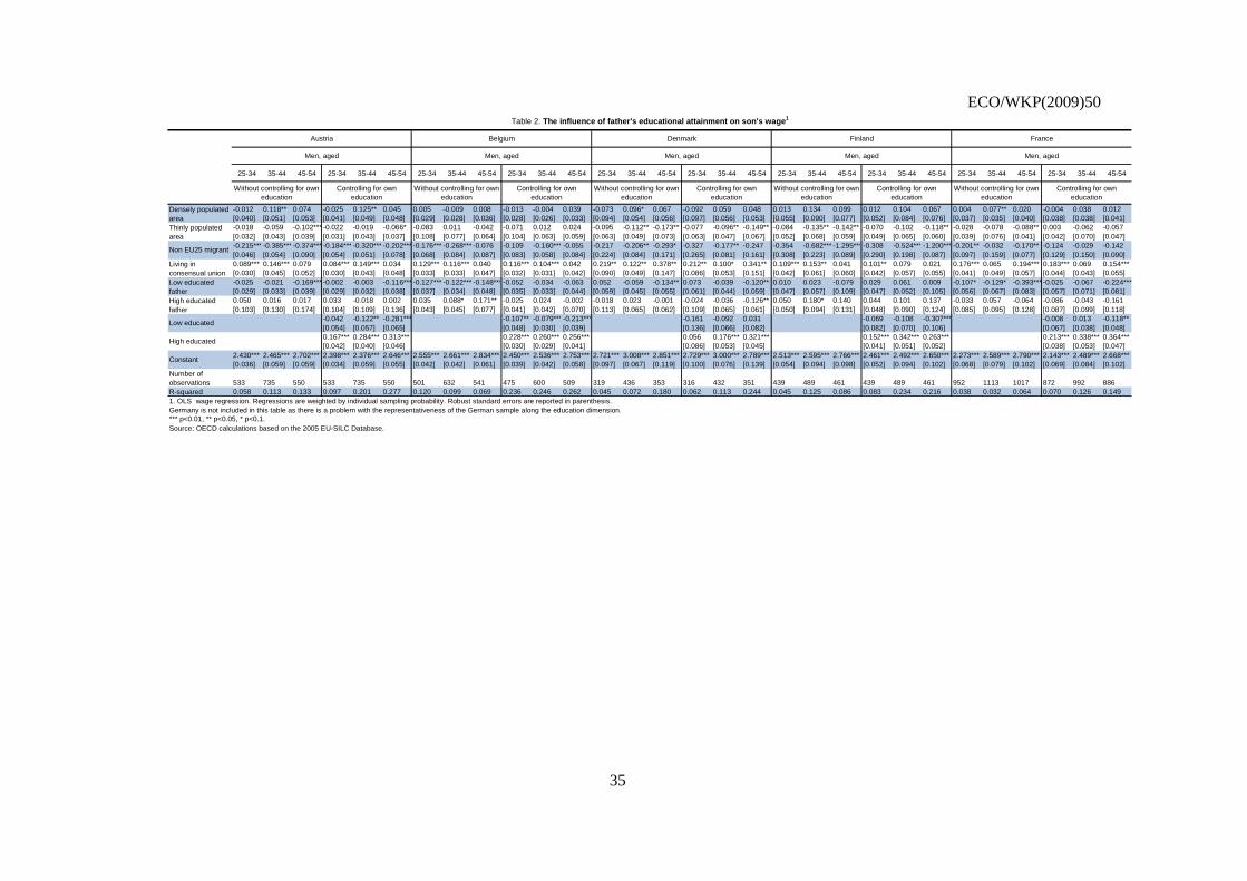
ECO/WKP(2009)50

35

25-34 35-44 45-54 25-34 35-44 45-54 25-34 35-44 45-54 25-34 35-44 45-54 25-34 35-44 45-54 25-34 35-44 45-54 25-34 35-44 45-54 25-34 35-44 45-54 25-34 35-44 45-54 25-34 35-44 45-54

-0.012 0.118** 0.074 -0.025 0.125** 0.045 0.005 -0.009 0.008 -0.013 -0.004 0.039 -0.073 0.096* 0.067 -0.092 0.059 0.048 0.013 0.134 0.099 0.012 0.104 0.067 0.004 0.077** 0.020 -0.004 0.038 0.012[0.040] [0.051] [0.053] [0.041] [0.049] [0.048] [0.029] [0.028] [0.036] [0.028] [0.026] [0.033] [0.094] [0.054] [0.056] [0.097] [0.056] [0.053] [0.055] [0.090] [0.077] [0.052] [0.084] [0.076] [0.037] [0.035] [0.040] [0.038] [0.038] [0.041]-0.018 -0.059 -0.102*** -0.022 -0.019 -0.066* -0.083 0.011 -0.042 -0.071 0.012 0.024 -0.095 -0.112** -0.173** -0.077 -0.096** -0.149** -0.084 -0.135** -0.142** -0.070 -0.102 -0.118** -0.028 -0.078 -0.088** 0.003 -0.062 -0.057[0.032] [0.043] [0.039] [0.031] [0.043] [0.037] [0.108] [0.077] [0.064] [0.104] [0.063] [0.059] [0.063] [0.049] [0.073] [0.063] [0.047] [0.067] [0.052] [0.068] [0.059] [0.049] [0.065] [0.060] [0.039] [0.076] [0.041] [0.042] [0.070] [0.047]-0.215*** -0.385*** -0.374*** -0.184*** -0.320*** -0.202*** -0.176*** -0.268*** -0.076 -0.109 -0.160*** -0.055 -0.217 -0.206** -0.293* -0.327 -0.177** -0.247 -0.354 -0.682*** -1.295*** -0.308 -0.524*** -1.200*** -0.201** -0.032 -0.170** -0.124 -0.029 -0.142[0.046] [0.054] [0.090] [0.054] [0.051] [0.078] [0.068] [0.084] [0.087] [0.083] [0.058] [0.084] [0.224] [0.084] [0.171] [0.265] [0.081] [0.161] [0.308] [0.223] [0.089] [0.290] [0.198] [0.087] [0.097] [0.159] [0.077] [0.129] [0.150] [0.090]0.089*** 0.146*** 0.079 0.084*** 0.149*** 0.034 0.129*** 0.116*** 0.040 0.116*** 0.104*** 0.042 0.219** 0.122** 0.378** 0.212** 0.100* 0.341** 0.109*** 0.153** 0.041 0.101** 0.079 0.021 0.176*** 0.065 0.194*** 0.183*** 0.069 0.154***[0.030] [0.045] [0.052] [0.030] [0.043] [0.048] [0.033] [0.033] [0.047] [0.032] [0.031] [0.042] [0.090] [0.049] [0.147] [0.086] [0.053] [0.151] [0.042] [0.061] [0.060] [0.042] [0.057] [0.055] [0.041] [0.049] [0.057] [0.044] [0.043] [0.055]-0.025 -0.021 -0.169*** -0.002 -0.003 -0.116*** -0.127*** -0.122*** -0.148*** -0.052 -0.034 -0.063 0.052 -0.059 -0.134** 0.073 -0.039 -0.120** 0.010 0.023 -0.079 0.029 0.061 0.009 -0.107* -0.129* -0.393*** -0.025 -0.067 -0.224***[0.029] [0.033] [0.039] [0.029] [0.032] [0.038] [0.037] [0.034] [0.048] [0.035] [0.033] [0.044] [0.059] [0.045] [0.055] [0.061] [0.044] [0.059] [0.047] [0.057] [0.109] [0.047] [0.052] [0.105] [0.056] [0.067] [0.083] [0.057] [0.071] [0.081]0.050 0.016 0.017 0.033 -0.018 0.002 0.035 0.088* 0.171** -0.025 0.024 -0.002 -0.018 0.023 -0.001 -0.024 -0.036 -0.126** 0.050 0.180* 0.140 0.044 0.101 0.137 -0.033 0.057 -0.064 -0.086 -0.043 -0.161[0.103] [0.130] [0.174] [0.104] [0.109] [0.136] [0.043] [0.045] [0.077] [0.041] [0.042] [0.070] [0.113] [0.065] [0.062] [0.109] [0.065] [0.061] [0.050] [0.094] [0.131] [0.048] [0.090] [0.124] [0.085] [0.095] [0.128] [0.087] [0.099] [0.118]

-0.042 -0.122** -0.281*** -0.107** -0.079*** -0.213*** -0.161 -0.092 0.031 -0.069 -0.108 -0.307*** -0.008 0.013 -0.118**[0.054] [0.057] [0.065] [0.048] [0.030] [0.039] [0.136] [0.066] [0.082] [0.082] [0.070] [0.106] [0.067] [0.038] [0.048]0.167*** 0.284*** 0.313*** 0.228*** 0.260*** 0.256*** 0.056 0.176*** 0.321*** 0.152*** 0.342*** 0.263*** 0.213*** 0.338*** 0.364***[0.042] [0.040] [0.046] [0.030] [0.029] [0.041] [0.086] [0.053] [0.045] [0.041] [0.051] [0.052] [0.038] [0.053] [0.047]

2.430*** 2.465*** 2.702*** 2.398*** 2.376*** 2.646*** 2.555*** 2.661*** 2.834*** 2.450*** 2.536*** 2.753*** 2.721*** 3.008*** 2.851*** 2.729*** 3.000*** 2.789*** 2.513*** 2.595*** 2.766*** 2.461*** 2.492*** 2.650*** 2.273*** 2.589*** 2.790*** 2.143*** 2.489*** 2.668***[0.036] [0.059] [0.059] [0.034] [0.059] [0.055] [0.042] [0.042] [0.061] [0.039] [0.042] [0.058] [0.097] [0.067] [0.119] [0.100] [0.076] [0.139] [0.054] [0.094] [0.098] [0.052] [0.094] [0.102] [0.068] [0.079] [0.102] [0.069] [0.084] [0.102]

533 735 550 533 735 550 501 632 541 475 600 509 319 436 353 316 432 351 439 489 461 439 489 461 952 1113 1017 872 992 886R-squared 0.058 0.113 0.133 0.097 0.201 0.277 0.120 0.099 0.069 0.236 0.246 0.262 0.045 0.072 0.180 0.062 0.113 0.244 0.045 0.125 0.086 0.083 0.234 0.216 0.038 0.032 0.064 0.070 0.126 0.149

Germany is not included in this table as there is a problem with the representativeness of the German sample along the education dimension.

Source: OECD calculations based on the 2005 EU-SILC Database.

Table 2. The influence of father's educational attainment on son's wage1

Austria Belgium Denmark Finland France

Men, aged

Without controlling for own education

Controlling for own education






Densely populated area

Men, aged Men, aged Men, aged Men, aged




High educated

Constant

1. OLS wage regression. Regressions are weighted by individual sampling probability. Robust standard errors are reported in parenthesis.

*** p<0.01, ** p<0.05, * p<0.1.

Thinly populated area

Non EU25 migrant

Living in consensual unionLow educated fatherHigh educated father

Low educated

Number of observations

ECO/WKP(2009)50

36

25-34 35-44 45-54 25-34 35-44 45-54 25-34 35-44 45-54 25-34 35-44 45-54 25-34 35-44 45-54 25-34 35-44 45-54 25-34 35-44 45-54 25-34 35-44 45-54 25-34 35-44 45-54 25-34 35-44 45-54

0.070* -0.279** 0.066 0.036 -0.068 0.174** 0.003 0.063 0.006 -0.036 0.062 -0.081 0.067*** 0.124*** 0.075** 0.059** 0.094*** 0.050* -0.021 -0.159* -0.268***0.003 -0.070 -0.263*** .. .. .. .. .. .. [0.037] [0.127] [0.117] [0.035] [0.125] [0.086] [0.077] [0.073] [0.086] [0.074] [0.067] [0.074] [0.025] [0.023] [0.030] [0.024] [0.022] [0.026] [0.068] [0.084] [0.083] [0.056] [0.077] [0.071] .. .. .. .. .. .. 0.000 -0.389*** -0.059 0.000 -0.138 0.134 -0.147 -0.137* -0.142* -0.147* -0.097 -0.132* 0.027 0.009 -0.077** 0.032 0.009 -0.059** 0.058 -0.107 -0.128* 0.042 -0.086 -0.147** .. .. .. .. .. .. [0.000] [0.126] [0.116] [0.000] [0.127] [0.084] [0.092] [0.074] [0.084] [0.089] [0.068] [0.076] [0.028] [0.027] [0.033] [0.027] [0.025] [0.028] [0.081] [0.084] [0.077] [0.074] [0.068] [0.069] .. .. .. .. .. .. -0.093 -0.420*** -0.468***-0.050 -0.367*** -0.526***-0.012 -0.273** 0.108 -0.099 -0.353*** -0.083 -0.131*** -0.305***-0.321***-0.078* -0.268***-0.343***-0.379***-0.440***-0.031 -0.165* -0.547***-0.079 0.077 -0.187** -0.357***0.131* -0.109* -0.275**[0.073] [0.071] [0.093] [0.066] [0.081] [0.090] [0.127] [0.135] [0.179] [0.127] [0.127] [0.192] [0.050] [0.045] [0.066] [0.047] [0.045] [0.081] [0.106] [0.150] [0.190] [0.099] [0.126] [0.154] [0.104] [0.077] [0.097] [0.078] [0.065] [0.108] 0.201*** 0.201*** 0.119 0.192*** 0.161*** 0.067 0.000 0.000 0.000 0.000 0.000 0.000 0.104*** 0.118*** 0.063* 0.122*** 0.113*** 0.097*** 0.011 -0.026 -0.287** -0.004 -0.040 -0.364*** 0.293*** 0.203*** 0.117 0.310*** 0.173*** 0.129 [0.038] [0.051] [0.088] [0.035] [0.049] [0.075] [0.000] [0.000] [0.000] [0.000] [0.000] [0.000] [0.023] [0.025] [0.033] [0.022] [0.023] [0.029] [0.067] [0.155] [0.120] [0.060] [0.154] [0.113] [0.080] [0.052] [0.106] [0.082] [0.046] [0.097] -0.078 -0.121* -0.222* -0.001 0.002 -0.019 -0.121 -0.331***-0.321*** -0.076 -0.150* -0.124 -0.129*** -0.192***-0.438***-0.053* -0.077* -0.116***-0.240***-0.309***-0.305***-0.100 -0.121* -0.148** 0.123 -0.164***-0.223***0.151* -0.071* -0.082 [0.059] [0.068] [0.115] [0.061] [0.060] [0.100] [0.103] [0.091] [0.114] [0.095] [0.086] [0.103] [0.027] [0.042] [0.051] [0.029] [0.042] [0.044] [0.067] [0.078] [0.076] [0.073] [0.068] [0.064] [0.080] [0.050] [0.078] [0.079] [0.043] [0.076] 0.135 -0.029 0.156 0.113 -0.108 0.061 0.052 -0.085 -0.094 -0.016 -0.164 -0.201 0.087 0.231*** 0.044 0.032 0.126 -0.006 0.174* 0.084 0.343** 0.001 -0.059 0.077 0.023 0.094 0.189** -0.012 0.016 0.110 [0.087] [0.109] [0.172] [0.078] [0.104] [0.146] [0.127] [0.126] [0.245] [0.130] [0.126] [0.245] [0.073] [0.086] [0.147] [0.071] [0.079] [0.135] [0.093] [0.176] [0.133] [0.080] [0.166] [0.129] [0.105] [0.074] [0.086] [0.106] [0.066] [0.081]

-0.048 -0.128*** -0.194*** -0.098 -0.090 -0.203*** -0.124***-0.163***-0.241*** -0.257***-0.386***-0.307*** -0.101** -0.108** -0.265***[0.039] [0.038] [0.044] [0.098] [0.069] [0.069] [0.023] [0.020] [0.023] [0.055] [0.066] [0.066] [0.049] [0.044] [0.049] 0.252*** 0.316*** 0.371*** 0.230*** 0.368*** 0.405*** 0.129*** 0.268*** 0.421*** 0.314*** 0.329*** 0.386*** 0.118* 0.401*** 0.307***[0.048] [0.047] [0.058] [0.079] [0.062] [0.081] [0.035] [0.035] [0.041] [0.089] [0.080] [0.075] [0.060] [0.047] [0.086]

1.682*** 2.315*** 2.234*** 1.587*** 1.959*** 1.919*** 2.792*** 3.193*** 3.248*** 2.681*** 2.937*** 3.057*** 2.232*** 2.396*** 2.812*** 2.198*** 2.357*** 2.558*** 2.872*** 3.334*** 3.501*** 2.787*** 3.228*** 3.450*** 2.364*** 2.897*** 3.071*** 2.305*** 2.721*** 2.907***[0.059] [0.141] [0.176] [0.065] [0.144] [0.149] [0.106] [0.085] [0.121] [0.100] [0.088] [0.116] [0.029] [0.046] [0.059] [0.031] [0.046] [0.053] [0.069] [0.076] [0.062] [0.074] [0.070] [0.056] [0.106] [0.059] [0.108] [0.112] [0.053] [0.108] 528 547 464 526 547 462 214 337 338 213 336 335 2078 2475 2080 2076 2473 2080 556 505 454 553 500 450 459 603 460 452 602 458

R-squared 0.105 0.121 0.148 0.193 0.265 0.350 0.059 0.137 0.066 0.144 0.296 0.284 0.060 0.153 0.144 0.100 0.257 0.341 0.156 0.165 0.200 0.304 0.336 0.373 0.089 0.097 0.076 0.114 0.311 0.248 Germany is not included in this table as there is a problem with the representativeness of the German sample along the education dimension.

".." refers to data unavailability.Source: OECD calculations based on the 2005 EU-SILC Database.

*** p<0.01, ** p<0.05, * p<0.1.

Table 2.The influence of father's educational attainment on son's wage1

(continued)

Greece Ireland Italy Luxembourg Netherlands

Men, aged Men, aged












Men, aged


Men, aged


Thinly populated area Non EU25 migrant

Living in consensual union Low educated fatherHigh educated father

Low educated

High educated

Constant

ECO/WKP(2009)50

37

25-34 35-44 45-54 25-34 35-44 45-54 25-34 35-44 45-54 25-34 35-44 45-54 25-34 35-44 45-54 25-34 35-44 45-54 25-34 35-44 45-54 25-34 35-44 45-54

0.097* 0.153*** 0.354*** 0.018 0.086* 0.220*** 0.065** 0.141*** 0.098** 0.029 0.079** 0.060 -0.037 0.048 0.118 -0.078 0.028 0.079 0.104* -0.042 -0.088 0.071 -0.046 -0.076[0.053] [0.058] [0.075] [0.047] [0.050] [0.057] [0.029] [0.033] [0.046] [0.028] [0.031] [0.040] [0.106] [0.105] [0.122] [0.109] [0.108] [0.113] [0.055] [0.061] [0.070] [0.051] [0.060] [0.065]0.024 -0.054 0.068 0.029 -0.032 0.053 -0.004 -0.072** -0.134*** -0.006 -0.038 -0.076* -0.045 -0.128 -0.124 -0.058 -0.110 -0.112 0.172 0.153 0.312* 0.154 0.215** 0.315*[0.054] [0.063] [0.075] [0.052] [0.054] [0.061] [0.032] [0.035] [0.049] [0.030] [0.031] [0.042] [0.079] [0.091] [0.105] [0.079] [0.087] [0.094] [0.125] [0.123] [0.170] [0.124] [0.107] [0.164]-0.189 0.338* -0.302** -0.087 0.092 -0.497 -0.192*** -0.351***-0.429*** -0.184***-0.339*** -0.472***-0.012 -0.238* -0.156 -0.098 -0.259** -0.164 -0.117* -0.039 -0.020 -0.133** -0.039 -0.006[0.124] [0.187] [0.144] [0.129] [0.245] [0.341] [0.056] [0.056] [0.082] [0.060] [0.057] [0.095] [0.140] [0.123] [0.119] [0.097] [0.123] [0.115] [0.066] [0.084] [0.101] [0.067] [0.076] [0.084]0.007 0.126* -0.023 0.071* 0.083 -0.005 0.132*** 0.186*** 0.103 0.133*** 0.166*** 0.109* 0.045 0.130* 0.076 0.028 0.112 0.076 0.084* 0.122* 0.128* 0.086* 0.095 0.132**[0.045] [0.072] [0.128] [0.041] [0.054] [0.094] [0.025] [0.037] [0.069] [0.024] [0.035] [0.058] [0.061] [0.069] [0.053] [0.060] [0.071] [0.051] [0.045] [0.068] [0.067] [0.044] [0.065] [0.063]-0.376*** -0.411** -0.710***-0.108 -0.007 -0.012 -0.136*** -0.177***-0.334*** -0.076* -0.031 -0.124* 0.047 -0.089 -0.061 0.065 -0.064 0.100 -0.082* -0.162*** -0.206***-0.075 -0.094* -0.105[0.099] [0.175] [0.212] [0.084] [0.188] [0.242] [0.037] [0.056] [0.072] [0.040] [0.048] [0.067] [0.064] [0.070] [0.101] [0.063] [0.074] [0.118] [0.050] [0.058] [0.070] [0.048] [0.054] [0.066]0.192 0.739*** 0.131 0.141 0.490** 0.053 0.087 0.196*** 0.241** 0.038 0.128** 0.151* -0.075 0.116 0.277** -0.115 0.091 0.272** 0.080 0.313*** 0.309*** 0.019 0.223*** 0.159[0.142] [0.201] [0.344] [0.136] [0.209] [0.340] [0.057] [0.076] [0.096] [0.055] [0.063] [0.089] [0.098] [0.104] [0.137] [0.099] [0.105] [0.134] [0.059] [0.077] [0.102] [0.059] [0.072] [0.097]

-0.220***-0.451*** -0.739*** -0.060** -0.167*** -0.260*** 0.044 -0.004 -0.063 -0.121 -0.334***-0.331***[0.055] [0.070] [0.097] [0.029] [0.031] [0.037] [0.053] [0.099] [0.054] [0.090] [0.077] [0.073]0.369*** 0.489*** 0.344*** 0.196*** 0.340*** 0.286*** 0.119* 0.135* 0.352*** 0.216*** 0.367*** 0.369***[0.078] [0.093] [0.116] [0.034] [0.036] [0.044] [0.065] [0.070] [0.068] [0.043] [0.048] [0.062]

1.675*** 1.769*** 2.157*** 1.515*** 1.763*** 2.060*** 1.950*** 2.047*** 2.381*** 1.880*** 1.945*** 2.256*** 2.496*** 2.723*** 2.786*** 2.479*** 2.679*** 2.578*** 2.607*** 2.796*** 2.884*** 2.529*** 2.653*** 2.735***[0.108] [0.192] [0.248] [0.100] [0.203] [0.257] [0.042] [0.069] [0.105] [0.047] [0.062] [0.094] [0.097] [0.112] [0.136] [0.094] [0.105] [0.139] [0.068] [0.096] [0.095] [0.068] [0.096] [0.090]

465 482 404 458 467 389 1469 1635 1277 1465 1621 1255 330 335 325 329 335 325 493 565 523 493 564 523R-squared 0.150 0.151 0.136 0.310 0.420 0.499 0.082 0.157 0.145 0.151 0.315 0.318 0.014 0.090 0.124 0.034 0.103 0.233 0.037 0.104 0.105 0.093 0.241 0.236

Germany is not included in this table as there is a problem with the representativeness of the German sample along the education dimension.*** p<0.01, ** p<0.05, * p<0.1.Source: OECD calculations based on the 2005 EU-SILC Database.


Portugal Spain Sweden United Kingdom

High educated

Constant


Non EU25 migrant

Living in consensual unionLow educated fatherHigh educated father

Low educated


Table 2. The influence of father's educational attainment on son's wage 1 (continued)


Men, aged Men, aged Men, aged Men, aged









ECO/WKP(2009)50

38

25-34 35-44 45-54 25-34 35-44 45-54 25-34 35-44 45-54 25-34 35-44 45-54 25-34 35-44 45-54 25-34 35-44 45-54 25-34 35-44 45-54 25-34 35-44 45-54 25-34 35-44 45-54 25-34 35-44 45-54

0.042 0.153*** 0.194*** 0.015 0.109*** 0.060 -0.041 0.057* -0.050 -0.048 0.057** -0.057 0.190** 0.152*** 0.067 0.120 0.145*** 0.060 -0.082 0.197** 0.088 -0.099 0.195*** 0.093 0.061 0.066* 0.047 0.056 0.012 0.042(0.050) (0.043) (0.056) (0.050) (0.041) (0.046) (0.034) (0.032) (0.048) (0.030) (0.026) (0.043) (0.084) (0.056) (0.074) (0.085) (0.053) (0.069) (0.095) (0.081) (0.088) (0.093) (0.075) (0.076) (0.047) (0.036) (0.045) (0.047) (0.040) (0.041)-0.055 -0.025 -0.156*** -0.032 -0.003 -0.098** -0.177** 0.060 -0.231** -0.144** 0.063 -0.220** 0.082 -0.148*** 0.072 0.070 -0.116** 0.060 -0.167* -0.025 -0.066 -0.172* -0.016 -0.057 -0.055 -0.174*** -0.051 -0.040 -0.129** -0.049(0.048) (0.055) (0.055) (0.045) (0.066) (0.046) (0.083) (0.084) (0.109) (0.062) (0.083) (0.101) (0.087) (0.057) (0.070) (0.086) (0.053) (0.066) (0.092) (0.085) (0.082) (0.090) (0.079) (0.072) (0.059) (0.047) (0.063) (0.060) (0.054) (0.058)-0.147 -0.342*** -0.523*** -0.095 -0.217*** -0.228*** 0.141 -0.350*** -0.145 -0.057 -0.250*** -0.252*** -0.203 0.033 -0.047 -0.180 -0.005 -0.007 0.540** -0.324* 0.329 0.634** -0.220 0.345 0.172 -0.230*** 0.005 0.189 0.017 -0.050(0.107) (0.068) (0.089) (0.090) (0.063) (0.075) (0.101) (0.085) (0.112) (0.089) (0.064) (0.083) (0.221) (0.137) (0.182) (0.212) (0.130) (0.157) (0.255) (0.168) (0.305) (0.251) (0.178) (0.225) (0.146) (0.086) (0.098) (0.173) (0.098) (0.102)-0.049 -0.040 -0.071 -0.014 -0.041 0.000 0.085** -0.029 0.031 0.084*** -0.028 0.051 -0.040 0.087 -0.099 -0.074 0.078 -0.079 0.090 0.042 -0.124** 0.068 0.043 -0.100* 0.021 -0.011 0.043 0.039 0.002 0.011(0.046) (0.041) (0.049) (0.043) (0.046) (0.039) (0.038) (0.042) (0.054) (0.032) (0.037) (0.047) (0.073) (0.067) (0.077) (0.072) (0.063) (0.069) (0.070) (0.064) (0.063) (0.068) (0.060) (0.058) (0.051) (0.039) (0.052) (0.049) (0.043) (0.041)0.021 -0.086** -0.127*** 0.036 -0.016 -0.032 0.011 -0.056 -0.068 0.051 0.033 -0.018 -0.105 0.058 -0.124** -0.034 0.067 -0.092* -0.036 0.057 0.023 -0.040 0.050 0.049 -0.106 -0.118 -0.114 -0.107 -0.066 -0.188**(0.039) (0.036) (0.046) (0.036) (0.034) (0.038) (0.041) (0.042) (0.072) (0.035) (0.034) (0.047) (0.073) (0.053) (0.059) (0.071) (0.053) (0.054) (0.071) (0.057) (0.073) (0.070) (0.054) (0.067) (0.067) (0.073) (0.179) (0.067) (0.076) (0.079)0.209 0.113 0.302*** 0.117 0.085 0.106 0.141*** 0.119** 0.039 0.062 0.046 -0.020 -0.032 -0.102 0.129 -0.079 -0.111 0.074 -0.087 0.170** 0.276* -0.113 0.067 0.236* -0.093 0.038 0.294 -0.088 0.042 -0.007(0.149) (0.116) (0.114) (0.133) (0.084) (0.102) (0.047) (0.049) (0.089) (0.045) (0.044) (0.073) (0.089) (0.076) (0.092) (0.089) (0.074) (0.087) (0.096) (0.080) (0.144) (0.094) (0.079) (0.136) (0.082) (0.109) (0.197) (0.079) (0.109) (0.110)

-0.234*** -0.297*** -0.197*** -0.144*** -0.130*** 0.029 -0.275** -0.139* -0.067 0.226* 0.030 0.071 -0.119 -0.058 -0.193***(0.075) (0.079) (0.058) (0.048) (0.041) (0.069) (0.129) (0.082) (0.068) (0.123) (0.092) (0.075) (0.103) (0.057) (0.046)0.231*** 0.290*** 0.444*** 0.262*** 0.268*** 0.261*** 0.164** 0.068 0.140** 0.177*** 0.258*** 0.243*** 0.079* 0.269*** 0.276***(0.052) (0.045) (0.054) (0.033) (0.033) (0.048) (0.069) (0.046) (0.061) (0.066) (0.053) (0.051) (0.047) (0.044) (0.044)

2.349*** 2.342*** 2.313*** 2.260*** 2.308*** 2.495*** 2.550*** 2.682*** 2.884*** 2.306*** 2.513*** 2.790*** 2.563*** 2.921*** 3.131*** 2.558*** 2.903*** 3.066*** 2.541*** 2.452*** 2.747*** 2.462*** 2.331*** 2.569*** 2.505*** 2.461*** 2.680*** 2.445*** 2.512*** 2.749***(0.050) (0.061) (0.066) (0.048) (0.075) (0.067) (0.046) (0.067) (0.167) (0.048) (0.054) (0.077) (0.091) (0.076) (0.083) (0.099) (0.071) (0.082) (0.106) (0.088) (0.090) (0.105) (0.088) (0.084) (0.079) (0.080) (0.189) (0.088) (0.091) (0.092)

-0.004 -0.099 0.233* 0.009 -0.093 0.227 -0.084 0.065 0.129 -0.140 0.067 0.173 0.445** 0.163 -0.050 0.300 0.138 0.005 0.421** 0.469** 0.139 0.393** 0.472** 0.239 -0.029 0.211** 0.081 -0.051 0.237** 0.171*(0.161) (0.133) (0.134) (0.165) (0.136) (0.139) (0.128) (0.104) (0.110) (0.136) (0.112) (0.111) (0.216) (0.190) (0.197) (0.220) (0.196) (0.206) (0.190) (0.200) (0.219) (0.196) (0.195) (0.222) (0.102) (0.088) (0.086) (0.109) (0.095) (0.100)-0.113 -0.459*** -0.086 -0.089 -0.413*** 0.003 0.334 -0.280 0.181 0.243 -0.337 0.223 -0.097 0.134 -0.568*** -0.210 0.153 -0.523*** 0.217 0.345* -0.131 0.212 0.405** 0.071 0.097 0.062 -0.165 0.121 0.048 -0.082(0.145) (0.116) (0.118) (0.145) (0.117) (0.122) (0.350) (0.227) (0.249) (0.390) (0.247) (0.238) (0.209) (0.164) (0.182) (0.205) (0.175) (0.179) (0.163) (0.177) (0.189) (0.164) (0.174) (0.179) (0.125) (0.116) (0.119) (0.133) (0.120) (0.135)-0.353 -0.265* -0.509*** -0.240 -0.080 -0.155 -1.149*** -1.038*** -0.489** -1.045*** -1.078*** -0.116 -0.628 -0.655* 0.330 -0.676 -0.468 0.463 -1.427*** -0.565 -1.240** -1.351*** -0.522 -1.329*** -0.791*** -0.765*** -0.594*** -0.696*** -0.591*** -0.468**(0.224) (0.156) (0.192) (0.239) (0.165) (0.201) (0.210) (0.176) (0.236) (0.242) (0.248) (0.250) (0.408) (0.338) (0.617) (0.415) (0.365) (0.685) (0.520) (0.375) (0.512) (0.523) (0.387) (0.509) (0.174) (0.133) (0.141) (0.213) (0.175) (0.188)-0.374** -0.169 -0.102 -0.408** -0.185 -0.099 0.221 0.208* 0.140 0.071 0.229* 0.185 0.525** -0.175 0.450** 0.419* -0.185 0.442** -0.106 -0.398** 0.236 -0.121 -0.514*** 0.211 0.247* -0.020 -0.271** 0.092 -0.084 -0.244*(0.172) (0.129) (0.125) (0.171) (0.130) (0.131) (0.149) (0.123) (0.115) (0.152) (0.129) (0.116) (0.216) (0.191) (0.185) (0.220) (0.197) (0.185) (0.168) (0.179) (0.145) (0.166) (0.170) (0.148) (0.127) (0.111) (0.109) (0.135) (0.119) (0.132)-0.104 -0.094 -0.034 -0.059 0.008 0.103 -0.171 -0.412*** -0.405*** 0.075 -0.093 -0.165 0.152 -0.120 0.154 0.258 -0.108 0.149 0.095 -0.404** -0.226 0.117 -0.264 -0.154 -0.064 0.000 -0.152 0.211 0.179 0.184(0.122) (0.108) (0.105) (0.123) (0.114) (0.109) (0.152) (0.126) (0.125) (0.158) (0.140) (0.137) (0.193) (0.154) (0.154) (0.201) (0.163) (0.160) (0.148) (0.177) (0.207) (0.150) (0.185) (0.222) (0.141) (0.149) (0.242) (0.145) (0.163) (0.195)-0.807*** -0.085 0.194 -0.838*** -0.121 0.069 0.085 0.109 0.392* -0.077 -0.047 0.154 0.179 0.291 -0.157 0.091 0.256 -0.245 0.546*** -0.179 -0.015 0.507*** -0.163 -0.099 0.384** -0.133 0.032 0.350** -0.160 0.167(0.243) (0.228) (0.282) (0.250) (0.246) (0.297) (0.181) (0.174) (0.210) (0.189) (0.196) (0.202) (0.221) (0.235) (0.239) (0.215) (0.238) (0.247) (0.180) (0.216) (0.378) (0.180) (0.226) (0.412) (0.178) (0.198) (0.292) (0.178) (0.216) (0.256)-1.243*** -0.295** -0.109 -1.211*** -0.338*** -0.179* -0.453*** -0.119 0.308*** -0.277* -0.198 0.167* -0.422** 0.584*** 0.005 -0.368* 0.520*** 0.036 -0.762*** 0.043 0.217** -0.725*** 0.008 0.072 -0.534*** -0.192 0.219*** -0.400*** -0.093 0.163**(0.147) (0.125) (0.099) (0.146) (0.131) (0.108) (0.138) (0.129) (0.105) (0.148) (0.146) (0.097) (0.191) (0.139) (0.114) (0.198) (0.161) (0.113) (0.149) (0.148) (0.104) (0.151) (0.154) (0.101) (0.107) (0.125) (0.064) (0.112) (0.118) (0.077)

-0.466** -0.555*** -0.590*** -0.630*** -0.335** -0.729*** -0.895*** -0.198 -0.197 -0.337 -0.514** -0.120 -0.187 -0.250** -0.162*(0.182) (0.125) (0.122) (0.186) (0.134) (0.123) (0.266) (0.249) (0.183) (0.265) (0.251) (0.182) (0.191) (0.125) (0.098)0.013 0.075 0.497*** 0.618*** 0.787*** 0.313** -0.105 -0.029 0.150 0.027 0.289* 0.554*** 0.466*** 0.398*** 0.227(0.164) (0.149) (0.185) (0.148) (0.127) (0.135) (0.181) (0.164) (0.185) (0.139) (0.153) (0.153) (0.107) (0.097) (0.149)

1.606*** 1.230*** 0.600*** 1.632*** 1.302*** 0.594*** 1.020*** 0.753*** 0.103 0.772*** 0.474** 0.100 0.541** 0.624*** 0.640*** 0.868*** 0.748*** 0.615** 0.759*** 1.175*** 0.784*** 0.759*** 1.064*** 0.484* 0.778*** 0.845*** 0.886*** 0.477** 0.652*** 0.629***(0.219) (0.172) (0.147) (0.222) (0.179) (0.168) (0.168) (0.178) (0.158) (0.199) (0.203) (0.180) (0.248) (0.212) (0.199) (0.257) (0.231) (0.252) (0.232) (0.226) (0.229) (0.247) (0.239) (0.249) (0.176) (0.193) (0.261) (0.204) (0.213) (0.218)

615 859 745 615 859 745 627 839 737 596 772 680 395 537 419 392 534 419 546 624 719 546 623 719 1141 1441 1341 1032 1238 1149

270 262 243 270 262 243 156 264 330 139 224 292 68 60 63 67 57 63 164 114 142 164 113 142 349 382 366 280 274 265Log likelihood -435.3 -729.2 -658.9 -353.0 -514.9 -539.9 -420.6 -409.3 -336.5 -535.8 -550.0 -605.2 -1054 -1231 -1136Model degrees of freedom 8 8 8 8 8 8 8 8 8 7 8 8 8 8 8Rho (selectivity effect) -0.124 0.0489 -0.604 0.0836 -0.255 -0.770 0.191 -0.921 -0.936 -0.897 -0.905 -0.921 -0.813 -0.832 -0.841


Table 3. The influence of father's educational attainment on daughter's wage1

Austria Belgium Denmark Finland France


Wage rate

Women, aged Women, aged Women, aged Women, aged Women, aged






High educated father





Densely populated area Thinly populated area

Non EU25 migrant

Living in consensual union

Low educated father


Low educated

High educated

Constant

Employed (selection equation)


Non EU25 migrant


Low educated father

1. Wage regression model with selection into paid employment. Heckmann full maximum likelihood estimation. Regressions are weighted by individual sampling probability. Robust standard errors are reported in parenthesis.*** p<0.01, ** p<0.05, * p<0.1.

Offspring

Low educated

High educated

Constant

Number of observationsNumber of censored observations

ECO/WKP(2009)50

39

25-34 35-44 45-54 25-34 35-44 45-54 25-34 35-44 45-54 25-34 35-44 45-54 25-34 35-44 45-54 25-34 35-44 45-54 25-34 35-44 45-54 25-34 35-44 45-54 25-34 35-44 45-54 25-34 35-44 45-54

-0.041 0.131 -1.367***-0.266* 0.024 -0.855***0.069 0.107 0.171** 0.020 0.035 0.092 0.059** 0.116*** 0.016 0.058** 0.085*** 0.009 0.239 -0.135 -0.325***0.221 -0.097 -0.332*** .. .. .. .. .. .. (0.085) (0.320) (0.232) (0.153) (0.125) (0.167) (0.073) (0.068) (0.079) (0.068) (0.059) (0.065) (0.025) (0.028) (0.032) (0.024) (0.025) (0.027) (0.189) (0.110) (0.099) (0.172) (0.096) (0.081) .. .. .. .. .. .. -0.168** 0.007 -1.499***-0.356** -0.034 -0.949***0.118 0.036 -0.050 0.108 -0.099 -0.058 -0.017 -0.118***-0.040 -0.020 -0.067* -0.015 0.389** 0.069 -0.143 0.337** 0.031 -0.183* .. .. .. .. .. .. (0.076) (0.346) (0.225) (0.152) (0.131) (0.163) (0.080) (0.076) (0.101) (0.074) (0.076) (0.086) (0.032) (0.044) (0.052) (0.031) (0.038) (0.043) (0.171) (0.153) (0.125) (0.138) (0.109) (0.111) .. .. .. .. .. .. -0.159** -0.585***-0.630***-0.106 -0.365*** -0.592***0.009 0.403 -0.057 0.005 0.020 -0.147** -0.207***-0.331***-0.220** -0.164***-0.282***-0.181** -0.507 -0.235 -0.150 -0.586 -0.222 0.006 -0.108 -0.290* -0.064 -0.108 -0.290* -0.064(0.080) (0.078) (0.132) (0.079) (0.075) (0.130) (0.129) (0.247) (0.211) (0.147) (0.225) (0.071) (0.042) (0.057) (0.095) (0.040) (0.051) (0.082) (0.367) (0.260) (0.142) (0.368) (0.246) (0.165) [0.247] [0.167] [0.085] [0.247] [0.167] [0.085]0.146*** 0.017 0.251*** 0.198*** -0.035 0.192** .. .. .. .. .. .. 0.078*** 0.038 0.119* 0.079*** 0.053* 0.154*** 0.141 -0.114 -0.099 0.146 -0.046 -0.175 0.051 0.105 0.008 0.051 0.105 0.008 (0.046) (0.108) (0.097) (0.044) (0.060) (0.089) .. .. .. .. .. .. (0.024) (0.032) (0.069) (0.023) (0.030) (0.031) (0.127) (0.227) (0.114) (0.118) (0.091) (0.130) [0.051] [0.066] [0.075] [0.051] [0.066] [0.075] -0.045 -0.269***-0.261* 0.037 -0.057 -0.101 0.003 -0.352***-0.487***0.043 -0.263*** -0.180 -0.120***-0.176***-0.179** -0.057** -0.028 -0.017 -0.302** -0.264***-0.283** -0.177 -0.147* -0.081 -0.086* -0.071 -0.134 -0.086* -0.071 -0.134(0.063) (0.102) (0.157) (0.064) (0.069) (0.118) (0.080) (0.084) (0.085) (0.071) (0.083) (0.115) (0.027) (0.035) (0.082) (0.028) (0.033) (0.045) (0.126) (0.089) (0.112) (0.108) (0.076) (0.112) [0.046] [0.054] [0.084] [0.046] [0.054] [0.084] 0.167** 0.086 0.325 0.134* -0.001 0.399** 0.162* -0.017 -0.043 0.137 -0.244** -0.105 0.022 0.280*** 0.144* -0.027 0.178*** 0.115 0.136 0.131 0.281** 0.003 -0.171 0.001 0.004 0.123** 0.161** 0.004 0.123** 0.161**(0.078) (0.113) (0.211) (0.080) (0.096) (0.193) (0.086) (0.102) (0.163) (0.087) (0.113) (0.144) (0.063) (0.074) (0.087) (0.064) (0.068) (0.086) (0.174) (0.187) (0.133) (0.179) (0.161) (0.114) [0.049] [0.061] [0.079] [0.049] [0.061] [0.079]

-0.071 -0.377*** -0.265*** -0.339***-0.305*** -0.242*** -0.173***-0.311***-0.133*** -0.436***-0.302***-0.227**(0.058) (0.059) (0.082) (0.082) (0.061) (0.084) (0.034) (0.038) (0.038) (0.144) (0.089) (0.099)0.224*** 0.533*** 0.326*** 0.326*** 0.589*** 0.554*** 0.144*** 0.247*** 0.295*** 0.228** 0.406*** 0.590***(0.053) (0.048) (0.092) (0.075) (0.068) (0.067) (0.031) (0.037) (0.039) (0.105) (0.104) (0.088)

1.780*** 2.000*** 3.784*** 1.904*** 1.802*** 3.072*** 2.591*** 2.964*** 3.092*** 2.377*** 2.562*** 2.759*** 2.129*** 2.324*** 2.598*** 2.072*** 2.247*** 2.478*** 2.543*** 3.071*** 3.166*** 2.510*** 2.924*** 3.109*** 2.685*** 2.734*** 2.783*** 2.685*** 2.734*** 2.783***(0.107) (0.307) (0.307) (0.178) (0.140) (0.249) (0.090) (0.093) (0.156) (0.110) (0.102) (0.134) (0.042) (0.047) (0.074) (0.043) (0.052) (0.053) (0.135) (0.357) (0.143) (0.135) (0.109) (0.148) [0.050] [0.082] [0.105] [0.050] [0.082] [0.105]

1.248** -5.822 1.095* 1.339** -6.322 1.264** 0.298 -0.105 -0.021 0.143 -0.123 -0.108 -0.006 0.093 -0.012 -0.010 0.030 -0.045 -0.257 0.082 -0.225 -0.183 0.098 -0.274 .. .. .. .. .. .. (0.631) (0.000) (0.656) (0.657) (0.000) (0.556) (0.198) (0.153) (0.150) (0.206) (0.150) (0.155) (0.071) (0.063) (0.067) (0.071) (0.065) (0.069) (0.251) (0.197) (0.179) (0.268) (0.189) (0.183) .. .. .. .. .. .. 1.015 -6.133***0.960 1.173* -6.503*** 1.193** -0.286 -0.420***-0.207 -0.403* -0.472*** -0.239 -0.097 0.051 -0.126 -0.092 0.112 -0.048 -0.537* -0.309 -0.149 -0.553* -0.285 -0.158 .. .. .. .. .. .. (0.631) (0.106) (0.654) (0.657) (0.113) (0.554) (0.213) (0.152) (0.150) (0.215) (0.152) (0.156) (0.082) (0.076) (0.085) (0.083) (0.081) (0.084) (0.321) (0.219) (0.237) (0.330) (0.211) (0.232) .. .. .. .. .. .. -0.440** -0.001 0.701*** -0.396* 0.077 0.741*** -0.828** -0.485 1.345** -0.885** -0.797** 1.245** -0.287** -0.211 0.203 -0.206* -0.215 0.099 -1.473*** -0.228 -0.480 -1.570***-0.319 -0.475 -1.264*** -0.655* 0.061 -1.264***-0.655* 0.061 (0.212) (0.189) (0.234) (0.215) (0.224) (0.261) (0.330) (0.422) (0.544) (0.349) (0.380) (0.518) (0.115) (0.131) (0.182) (0.118) (0.144) (0.202) (0.257) (0.376) (0.344) (0.268) (0.317) (0.374) [0.296] [0.337] [0.331] [0.296] [0.337] [0.331] -0.320** -0.664***-0.561***-0.358*** -0.686*** -0.586*** .. .. .. .. .. .. -0.093 -0.309***-0.536***-0.095 -0.271***-0.459*** 0.516* 0.540** 0.536 0.499* 0.574** 0.530 0.331 0.103 -0.116 0.331 0.103 -0.116(0.139) (0.170) (0.148) (0.135) (0.169) (0.154) .. .. .. .. .. .. (0.073) (0.076) (0.076) (0.073) (0.083) (0.076) (0.300) (0.267) (0.344) (0.301) (0.258) (0.344) [0.239] [0.160] [0.175] [0.239] [0.160] [0.175] -0.221 -0.500** -0.501** -0.102 -0.058 -0.046 -0.164 -0.357* -0.169 -0.046 -0.134 0.344 -0.108 -0.396***-0.603***0.057 -0.066 -0.091 -0.689*** 0.019 0.323* -0.468* 0.046 0.471** -0.308* -0.206 -0.597***-0.308* -0.206 -0.597***(0.159) (0.221) (0.232) (0.162) (0.232) (0.249) (0.280) (0.182) (0.277) (0.317) (0.191) (0.303) (0.085) (0.095) (0.118) (0.090) (0.102) (0.128) (0.229) (0.183) (0.186) (0.245) (0.179) (0.210) [0.172] [0.136] [0.183] [0.172] [0.136] [0.183] 0.143 -0.106 -0.964***0.018 -0.192 -0.900** 0.702* -0.106 0.118 0.553 -0.284 0.022 0.356** -0.022 0.224 0.387** -0.241 0.111 -0.684** 0.244 0.575* -0.952***0.073 0.401 0.218 -0.004 0.043 0.218 -0.004 0.043 (0.224) (0.310) (0.341) (0.228) (0.312) (0.372) (0.375) (0.262) (0.390) (0.390) (0.277) (0.412) (0.178) (0.176) (0.221) (0.177) (0.180) (0.257) (0.319) (0.366) (0.305) (0.322) (0.342) (0.326) [0.199] [0.185] [0.270] [0.199] [0.185] [0.270] -0.293** 0.269* 0.585*** -0.115 0.112 0.291** -1.516***-0.594***-0.026 -1.379***-0.353* -0.091 -0.633***-0.453***0.035 -0.574***-0.458***-0.158*** -1.428*** -0.862***-0.151 -1.320***-0.857***-0.207 -1.395*** -0.751*** -0.023 -1.395***-0.751***-0.023(0.132) (0.162) (0.108) (0.124) (0.144) (0.136) (0.188) (0.188) (0.147) (0.207) (0.198) (0.131) (0.071) (0.074) (0.108) (0.071) (0.079) (0.060) (0.220) (0.267) (0.168) (0.229) (0.192) (0.171) [0.190] [0.151] [0.180] [0.190] [0.151] [0.180]

-0.477*** -0.660*** -0.417*** -0.452** -0.451*** -0.533*** -0.610***-0.629***-0.819*** -0.237 0.072 -0.112(0.138) (0.130) (0.131) (0.224) (0.139) (0.144) (0.071) (0.064) (0.068) (0.247) (0.183) (0.196)0.537*** 0.684*** 0.979*** 0.712*** 0.587*** 0.575*** -0.116 0.496*** 0.743*** 0.687*** 0.324 0.544**(0.135) (0.147) (0.182) (0.198) (0.168) (0.190) (0.099) (0.103) (0.134) (0.263) (0.224) (0.255)

-0.394 6.932*** -0.664 -0.732 7.181*** -1.075* 1.722*** 1.131*** 0.366 1.502*** 0.791*** 0.133 0.602*** 1.000*** 0.893*** 0.667*** 0.938*** 0.877*** 2.529*** 1.100*** 0.078 2.226*** 0.995*** 0.020 1.452*** 0.831*** 0.686*** 1.452*** 0.831*** 0.686***(0.650) (0.269) (0.714) (0.681) (0.275) (0.636) (0.366) (0.261) (0.311) (0.409) (0.297) (0.342) (0.098) (0.111) (0.142) (0.107) (0.120) (0.153) (0.314) (0.287) (0.218) (0.344) (0.253) (0.231) [0.233] [0.197] [0.216] [0.233] [0.197] [0.216]

799 834 758 796 829 753 420 724 691 417 717 685 3031 3629 3163 3023 3625 3155 593 602 565 586 599 559 560 725 583 560 725 583

376 392 491 373 387 487 142 313 317 139 307 313 1317 1657 1669 1309 1654 1661 180 218 289 177 217 285 155 285 212 155 285 212Log likelihood -657.2 -686.0 -566.4 -291.2 -607.6 -664.9 -2476 -3024 -2455 -622.4 -654.1 -585.8 -448.5 -692.0 -598.9Model degrees of freedom 7 8 7 7 7 7 8 8 8 8 8 8 4 4 4 Rho (selectivity effect) -0.646 0.457 -0.716 0.240 0.840 0.0739 0.261 0.169 -0.722 -0.159 0.0100 0.0318 0.163 -0.0134 0.0205

".." refers to data unavailability.Source: OECD calculations based on the 2005 EU-SILC Database.

Table 3. The influence of father's educational attainment on daughter's wage 1 (continued)

Greece Ireland Italy Luxembourg


Women, aged Women, aged Women, aged Women, aged Without controlling for own

educationControlling for own

educationWithout controlling for own

education







Non EU25 migrant


Low educated father

Low educated father


Low educated

High educated

Constant


Number of observationsNumber of censored observations

*** p<0.01, ** p<0.05, * p<0.1.

Netherlands

Without controlling for own

educationControlling for own

education

Wage rate


1. Wage regression model with selection into paid employment. Heckmann full maximum likelihood estimation. Regressions are weighted by individual sampling probability. Robust standard errors are reported in parenthesis.

Offspring

Low educated

High educated

Constant

Non EU25 migrant


ECO/WKP(2009)50

40

25-34 35-44 45-54 25-34 35-44 45-54 25-34 35-44 45-54 25-34 35-44 45-54 25-34 35-44 45-54 25-34 35-44 45-54 25-34 35-44 45-54 25-34 35-44 45-54

0.197*** 0.152** 0.279*** 0.130** 0.065 0.145** 0.079** 0.190*** 0.145*** 0.049 0.078* 0.098* 0.123 -0.221* 0.123 0.214 -0.171 0.109 -0.048 0.103* -0.006 -0.042 0.069 0.033(0.067) (0.068) (0.093) (0.051) (0.050) (0.057) (0.036) (0.058) (0.055) (0.032) (0.046) (0.050) (0.157) (0.128) (0.090) (0.167) (0.140) (0.087) (0.063) (0.057) (0.064) (0.060) (0.052) (0.062)0.150** -0.010 0.156 0.036 -0.034 0.075 0.025 -0.116* 0.015 0.025 -0.054 0.036 0.001 -0.154* -0.008 0.080 -0.140 -0.009 -0.057 0.019 -0.181 -0.063 -0.029 -0.133(0.076) (0.076) (0.097) (0.058) (0.054) (0.068) (0.046) (0.065) (0.065) (0.044) (0.052) (0.057) (0.148) (0.089) (0.079) (0.154) (0.102) (0.079) (0.184) (0.194) (0.120) (0.188) (0.191) (0.116)-0.026 -0.536** 0.614 -0.295***-0.468** 0.129 -0.304***-0.238***-0.300*** -0.247***-0.138** -0.253***-0.178 -0.230** -0.088 -0.220 -0.253** -0.132 0.067 0.117 0.144 0.056 0.070 0.108(0.145) (0.267) (0.418) (0.111) (0.234) (0.113) (0.070) (0.086) (0.081) (0.068) (0.067) (0.082) (0.297) (0.102) (0.147) (0.288) (0.122) (0.146) (0.085) (0.096) (0.106) (0.079) (0.086) (0.100)-0.079 -0.157* 0.218** 0.049 -0.069 0.188*** 0.169*** -0.062 0.059 0.178*** -0.034 0.119** -0.173 -0.076 0.011 -0.142 -0.166* 0.016 -0.014 -0.016 0.044 -0.008 -0.016 0.022(0.057) (0.082) (0.104) (0.046) (0.062) (0.071) (0.033) (0.055) (0.057) (0.032) (0.042) (0.049) (0.106) (0.074) (0.054) (0.107) (0.089) (0.054) (0.053) (0.052) (0.057) (0.051) (0.051) (0.053)-0.220* -0.680** -0.978***0.100 0.011 -0.589** -0.134***-0.336***-0.335*** -0.061 -0.061 -0.158** 0.153 -0.269***-0.086 0.147 -0.308** -0.097 -0.004 -0.095* -0.167***0.012 -0.082 -0.102(0.113) (0.272) (0.191) (0.109) (0.215) (0.275) (0.050) (0.103) (0.082) (0.046) (0.093) (0.075) (0.100) (0.094) (0.072) (0.103) (0.126) (0.070) (0.061) (0.056) (0.065) (0.059) (0.052) (0.067)0.011 0.115 -0.030 0.265** 0.104 -0.571* 0.020 0.220* 0.122 -0.004 0.034 0.026 0.153 -0.075 -0.019 0.163 -0.244 -0.036 0.087 0.149** 0.249** 0.045 0.087 0.172*(0.178) (0.304) (0.232) (0.133) (0.235) (0.294) (0.060) (0.120) (0.101) (0.058) (0.104) (0.092) (0.136) (0.139) (0.101) (0.132) (0.159) (0.097) (0.076) (0.075) (0.102) (0.074) (0.075) (0.098)

-0.387***-0.474*** -0.467*** -0.097* -0.331*** -0.103* -0.132 0.320** -0.012 -0.332***-0.316***-0.358***(0.065) (0.066) (0.100) (0.053) (0.044) (0.060) (0.237) (0.126) (0.112) (0.103) (0.103) (0.100)0.598*** 0.622*** 0.784*** 0.280*** 0.577*** 0.336*** -0.162* 0.096 0.063 0.184*** 0.257*** 0.202***(0.066) (0.089) (0.130) (0.036) (0.046) (0.060) (0.091) (0.083) (0.048) (0.055) (0.048) (0.055)

1.504*** 2.110*** 2.225*** 1.021*** 1.702*** 2.210*** 1.900*** 1.679*** 2.254*** 1.725*** 1.577*** 2.215*** 2.406*** 2.829*** 2.705*** 2.408*** 3.085*** 2.686*** 2.724*** 2.687*** 2.513*** 2.596*** 2.595*** 2.452***(0.133) (0.270) (0.216) (0.122) (0.235) (0.317) (0.057) (0.123) (0.106) (0.070) (0.113) (0.106) (0.176) (0.140) (0.100) (0.214) (0.176) (0.103) (0.082) (0.078) (0.119) (0.089) (0.074) (0.114)

0.274* 0.165 0.278** 0.088 0.064 0.206 0.020 0.194** 0.087 -0.019 0.077 0.010 -0.058 -0.146 -0.398 -0.033 0.134 -0.347 0.071 -0.092 0.055 0.124 -0.063 0.145(0.161) (0.137) (0.130) (0.157) (0.147) (0.134) (0.094) (0.081) (0.093) (0.096) (0.085) (0.094) (0.242) (0.315) (0.402) (0.293) (0.219) (0.424) (0.165) (0.132) (0.136) (0.165) (0.136) (0.144)-0.140 0.281* 0.086 -0.230 0.262* 0.080 -0.347***-0.227***-0.181* -0.287***-0.180** -0.132 -0.177 -0.176 -0.712** -0.027 -0.174 -0.644* -0.142 -0.359 -0.403* -0.092 -0.334 -0.404*(0.173) (0.146) (0.144) (0.166) (0.152) (0.150) (0.101) (0.087) (0.100) (0.102) (0.090) (0.104) (0.225) (0.259) (0.349) (0.201) (0.160) (0.363) (0.350) (0.282) (0.216) (0.337) (0.284) (0.229)-0.590* 0.432 0.159 -0.948***0.728 -0.283 -0.421** 0.032 0.106 -0.403** 0.250 -0.013 0.142 -0.102 -0.838** 0.257 -0.300 -0.579 -0.690***-0.636***-0.313 -0.592***-0.639***-0.355*(0.328) (0.495) (0.701) (0.313) (0.503) (0.542) (0.170) (0.155) (0.190) (0.185) (0.170) (0.212) (0.386) (0.308) (0.364) (0.415) (0.191) (0.385) (0.158) (0.160) (0.196) (0.164) (0.170) (0.196)-0.336* -0.149 -0.280* -0.100 -0.125 -0.396***-0.113 -0.307***-0.564*** -0.110 -0.372*** -0.544***0.516*** 0.285 0.196 0.610* 0.481*** 0.140 0.065 0.037 0.114 -0.008 -0.111 0.058(0.174) (0.171) (0.145) (0.179) (0.188) (0.152) (0.085) (0.086) (0.089) (0.088) (0.094) (0.091) (0.176) (0.217) (0.180) (0.353) (0.140) (0.190) (0.146) (0.126) (0.127) (0.152) (0.130) (0.132)-0.108 -0.095 -0.823* 0.206 0.795* -0.976 -0.170 -0.207 -0.177 0.051 0.036 0.407** 0.015 0.061 -0.066 0.113 -0.089 0.040 -0.309** -0.223* 0.057 -0.247 -0.131 0.312**(0.359) (0.335) (0.452) (0.421) (0.464) (0.846) (0.135) (0.142) (0.171) (0.140) (0.155) (0.168) (0.194) (0.261) (0.298) (0.171) (0.198) (0.298) (0.153) (0.125) (0.134) (0.158) (0.128) (0.143)1.026* 0.275 -0.306 0.906 0.264 -1.002 -0.080 0.296 0.456** -0.126 0.096 0.382* -0.036 0.508 0.238 -0.201 -0.123 0.188 0.108 -0.236 0.559** -0.005 -0.381** 0.460**(0.591) (0.479) (0.607) (0.607) (0.543) (0.948) (0.171) (0.182) (0.212) (0.172) (0.196) (0.204) (0.202) (0.366) (0.363) (0.271) (0.252) (0.353) (0.218) (0.162) (0.223) (0.223) (0.166) (0.227)-0.414** 0.124 0.190 -0.172 0.136 0.115 -0.679***-0.198***0.128* -0.518***-0.228*** -0.031 -0.280***0.369 0.285* -0.312 0.006*** 0.168 -1.535***-0.651***-0.159 -1.419***-0.570***-0.213*(0.178) (0.176) (0.124) (0.161) (0.165) (0.108) (0.080) (0.071) (0.077) (0.094) (0.086) (0.065) (0.107) (0.237) (0.160) (0.449) (0.000) (0.168) (0.150) (0.144) (0.119) (0.156) (0.147) (0.117)

-0.971***-0.839*** -0.329 -0.564***-0.461*** -0.678*** -0.592* -0.561***-0.247 -0.954***-0.794***-1.036***(0.192) (0.215) (0.212) (0.096) (0.081) (0.096) (0.309) (0.200) (0.278) (0.243) (0.184) (0.144)0.330 0.718** 0.673** 0.282** 0.553*** 0.602*** 0.098 0.332** 0.482** 0.186 0.395*** 0.208(0.350) (0.351) (0.278) (0.110) (0.101) (0.119) (0.162) (0.133) (0.204) (0.141) (0.120) (0.137)

1.351*** 0.579 0.875* 1.394*** 0.392 1.430 1.065*** 0.497*** 0.260 0.899*** 0.486** 0.192 0.716*** 0.577 1.405*** 0.565** 0.724** 1.241*** 1.779*** 1.525*** 0.496*** 1.662*** 1.455*** 0.538**(0.420) (0.374) (0.476) (0.447) (0.530) (0.911) (0.156) (0.173) (0.195) (0.177) (0.194) (0.196) (0.266) (0.407) (0.441) (0.260) (0.282) (0.441) (0.250) (0.197) (0.191) (0.277) (0.198) (0.216)

557 678 647 549 648 610 1922 2231 2045 1909 2203 1982 340 382 386 339 380 385 598 733 643 598 731 643

123 193 307 117 171 278 719 1126 1220 709 1102 1163 61 54 58 60 53 57 180 183 180 180 182 180Log likelihood -410.5 -552.0 -554.8 -1629 -1933 -1590 -379.0 -370.3 -269.4 -565.1 -770.2 -693.4Model degrees of freedom 8 8 8 8 8 8 0 0 8 8 8 8Rho (selectivity effect) 0.809 -0.696 -0.647 -0.443 0.786 -0.734 -1.000 -1.000 -0.777 -0.256 -0.361 0.272



Wage rate








Low educated

High educated

Constant

Spain Sweden United Kingdom Women, aged Women, aged Women, aged Women, aged




Portugal

Thinly populated area Non EU25 migrant

Living in consensual union Low educated father


Number of observations Number of censored observations

1. Wage regression model with selection into paid employment. Heckmann full maximum likelihood estimation. Regressions are weighted by individual sampling probability. Robust standard errors are reported in parenthesis.*** p<0.01, ** p<0.05, * p<0.1.

Table 3. The influence of father's educational attainment on daughter's wage 1

(continued)

Offspring Low educated

High educated

Constant

Non EU25 migrant

Living in consensual union Low educated father



ECO/WKP(2009)50

41

p25 p50 p75 p25 p50 p75

Austria 37.0 34.2 45.8 39.2 33.8 47.1Belgium 39.2 34.2 55.3 39.8 36.3 50.8Denmark 42.3 35.0 49.7 38.4 39.2 42.0Finland 38.4 44.7 60.0 35.9 32.3 52.0France 34.1 24.1 53.4 35.4 28.3 62.0Greece 33.1 23.9 33.5 37.8 34.8 55.6Ireland 39.5 20.5 41.6 40.9 40.6 70.4Italy 35.0 27.0 67.0 37.2 34.9 68.4Luxembourg 41.0 30.6 60.1 44.0 38.2 59.8Netherlands 39.3 29.6 51.8 38.3 37.5 49.7Portugal2 37.1 30.5 78.2 38.4 29.1 51.3Spain 36.2 27.2 63.9 37.5 37.8 59.9Sweden 36.0 27.3 53.8 37.6 21.1 53.1United Kingdom 40.7 30.2 57.9 36.8 29.8 43.0

Unweighted average 37.8 29.9 55.1 38.4 33.8 54.6

2. 25-34 years old for Portugal.



Table 4. Persistence in wages is higher at the top and the bottom1

35-44 years old

Men Women

1. This table reports the probability for the offspring to end up in the same wage quartile as the offspring's parent. Parental background is proxied by the highest level of education achieved by the offspring's father. Thus, the first column reports the probability of a son/daughter to end up in the lowest quartile (25th) conditional on his father having less than upper secondary education, the second column reports the probability of a son/daughter to end up in median wages conditional on his father having upper-secondary education, and the third column reports the probability of a son/daughter to end up in the highest quartile (75th) conditional on his father having tertiary education. If parental background had no influence on off springs' wages, the probability to end up in each quartile would be the same.

ECO/WKP(2009)50

42

Men Women Men Women

Austria 9.1 8.8 6.5Belgium 8.2 8.0 5.5 5.0Denmark 6.5 10.3 9.7 13.7Finland 7.5 8.5 10.2 12.3France 9.1 9.2 9.0 13.3Greece 10.4 7.5 11.1 9.9Ireland 6.7 9.2 9.1 9.1Italy 8.3 8.7 5.3 n.aLuxembourg 5.3 7.3 8.7 9.8Netherlands 7.4 7.6 6.9 7.5Portugal2 7.3 10.4 3.9 n.aSpain 8.5 9.0 1.8 4.4Sweden 6.9 6.6 9.8 12.5United Kingdom 5.8 8.1 3.3 8.7

Unweighted average 7.6 8.5 7.3 9.4

2. 25-34 years old for Portugal.


1. The bottom-to-top mobility reports the probability for the offspring to end up in the top wage percentile (90th) conditional on the offspring’s father having below upper-secondary education, while the top-to-bottom mobility reports the probability for the offspring to end up in the bottom wage percentile (10th) conditional on the offspring’s father having tertiary education.


Table 5. Long-distance mobility: Probability to move from the bottom to the top and

vice versa 1

35-44 years old

Bottom to top Top to bottom

ECO/WKP(2009)50

43

25th 50th 75th 25th 50th 75th 25th 50th 75th 25th 50th 75th 25th 50th 75th 25th 50th 75th 25th 50th 75th

0.051 0.066* 0.067 -0.007 0.021 -0.039 0.038 0.066* 0.068 0.172* 0.110 0.065 0.086** 0.053 0.109*** -0.415** -0.318***-0.128 0.036 0.051 0.081(0.041) (0.039) (0.084) (0.039) (0.029) (0.042) (0.055) (0.038) (0.053) (0.096) (0.074) (0.093) (0.041) (0.032) (0.040) (0.162) (0.108) (0.198) (0.056) (0.063) (0.120)-0.054 -0.051 -0.135* 0.010 -0.018 -0.007 -0.079 -0.104***-0.126** -0.126* -0.105* -0.208** -0.088* -0.140***-0.186***-0.599***-0.431***-0.226 -0.109* -0.119* -0.203(0.037) (0.034) (0.074) (0.096) (0.073) (0.098) (0.051) (0.035) (0.049) (0.076) (0.062) (0.081) (0.053) (0.042) (0.053) (0.162) (0.108) (0.197) (0.064) (0.068) (0.131)-0.328*** -0.318***-0.364***-0.133 -0.243*** -0.264***-0.190 -0.229** -0.283** -0.960*** -0.743***-0.510***-0.281***-0.198***-0.109 -0.405***-0.447***-0.460***-0.466***-0.280***-0.032(0.052) (0.047) (0.098) (0.083) (0.069) (0.098) (0.127) (0.090) (0.118) (0.194) (0.176) (0.179) (0.071) (0.061) (0.081) (0.063) (0.056) (0.123) (0.098) (0.091) (0.189)0.000 -0.004 -0.029 -0.069 -0.105*** -0.141***-0.050 -0.048 -0.064 -0.074 -0.052 0.097 -0.016 -0.064 -0.254***-0.130** -0.030 -0.157 -0.392***-0.306***-0.433***(0.032) (0.030) (0.064) (0.044) (0.034) (0.049) (0.049) (0.033) (0.045) (0.068) (0.061) (0.074) (0.075) (0.059) (0.074) (0.061) (0.055) (0.107) (0.070) (0.073) (0.157)-0.240** 0.204** 0.168 0.146** 0.145*** 0.090 0.012 0.082* 0.103* 0.104 0.222*** 0.365*** 0.057 0.115 0.019 0.052 0.065 -0.124 -0.218***-0.001 -0.197(0.096) (0.080) (0.163) (0.063) (0.047) (0.065) (0.062) (0.042) (0.059) (0.094) (0.078) (0.096) (0.103) (0.077) (0.092) (0.088) (0.084) (0.173) (0.084) (0.112) (0.207)0.103** 0.091** 0.136* 0.098** 0.109*** 0.056 0.060 0.072** 0.096* 0.093 0.188*** 0.175** 0.100* 0.106** 0.085 0.309*** 0.244*** 0.160** .. .. ..(0.040) (0.037) (0.082) (0.046) (0.037) (0.053) (0.050) (0.036) (0.050) (0.069) (0.058) (0.073) (0.054) (0.045) (0.061) (0.042) (0.038) (0.076) .. .. ..2.289*** 2.476*** 2.730*** 2.425*** 2.622*** 2.934*** 2.925*** 3.045*** 3.222*** 2.469*** 2.631*** 2.835*** 2.229*** 2.502*** 2.942*** 2.159*** 2.229*** 2.440*** 3.003*** 3.144*** 3.548***(0.047) (0.045) (0.097) (0.057) (0.044) (0.064) (0.059) (0.041) (0.059) (0.095) (0.087) (0.112) (0.091) (0.070) (0.087) (0.172) (0.117) (0.216) (0.068) (0.073) (0.145)

735 735 735 632 632 632 436 436 436 489 489 489 1113 1113 1113 547 547 547 337 337 337

".." refers to data unavailability.

Table 6. The influence of parental background on individuals' adult wages: quantile regressions

Austria Belgium Denmark Finland France Greece Ireland

Wage

High educated fatherLiving in consensual union

Constant

Wage


Low educated father

Wage Wage Wage Wage Wage

Non EU25 migrant


Men 35-44 years old. Quantile wage regressions based on quartiles of the corresponding distribution. Regressions are weighted by individual sampling probability. Robust standard errors are reported in parenthesis.

*** p<0.01, ** p<0.05, * p<0.1.



ECO/WKP(2009)50

44

25th 50th 75th 25th 50th 75th 25th 50th 75th 25th 50th 75th 25th 50th 75th 25th 50th 75th 25th 50th 75th

0.122*** 0.101*** 0.077*** -0.334***-0.270***-0.157* .. .. .. 0.118** 0.144** 0.156* 0.153*** 0.145*** 0.163*** 0.057 0.102 0.212** 0.054 -0.051 -0.060(0.017) (0.024) (0.021) (0.062) (0.062) (0.080) .. .. .. (0.058) (0.070) (0.093) (0.028) (0.030) (0.050) (0.110) (0.068) (0.087) (0.076) (0.070) (0.080)0.019 -0.013 -0.000 -0.145** -0.170** -0.163* .. .. .. -0.021 -0.086 -0.026 -0.053* -0.082** -0.062 -0.075 -0.126** -0.073 0.067 0.273* 0.172(0.020) (0.027) (0.025) (0.069) (0.069) (0.094) .. .. .. (0.067) (0.074) (0.096) (0.030) (0.032) (0.055) (0.094) (0.059) (0.076) (0.155) (0.143) (0.163)-0.287***-0.227***-0.295***-0.411***-0.744***-0.549***-0.153** -0.227** -0.245** 0.273 0.204 0.485* -0.288***-0.350***-0.413***-0.505***-0.177** -0.068 -0.136 -0.184* 0.150(0.037) (0.046) (0.038) (0.100) (0.120) (0.155) (0.074) (0.103) (0.113) (0.167) (0.231) (0.262) (0.051) (0.048) (0.083) (0.130) (0.075) (0.094) (0.104) (0.102) (0.112)-0.107***-0.145***-0.216***-0.303***-0.224***-0.324***-0.113***-0.098 -0.203***-0.235** -0.580***-0.597** -0.097* -0.232***-0.178** -0.121 0.018 -0.061 -0.152** -0.143** -0.220***(0.026) (0.035) (0.032) (0.060) (0.059) (0.077) (0.042) (0.060) (0.065) (0.103) (0.217) (0.256) (0.054) (0.058) (0.088) (0.107) (0.064) (0.071) (0.074) (0.069) (0.076)0.133*** 0.278*** 0.415*** 0.076 0.185* 0.247 0.112** 0.158** 0.077 0.997*** 0.643** 0.406 0.161** 0.132* 0.218** 0.015 0.136* 0.230** 0.284*** 0.334*** 0.380***(0.046) (0.063) (0.063) (0.100) (0.099) (0.153) (0.051) (0.073) (0.076) (0.153) (0.267) (0.348) (0.065) (0.069) (0.107) (0.128) (0.075) (0.090) (0.097) (0.092) (0.105)0.129*** 0.078*** 0.112*** -0.300***-0.109 -0.033 0.176*** 0.118** 0.160*** 0.072 0.125 0.131 0.166*** 0.144*** 0.143** 0.068 0.090* 0.147** 0.162** 0.201*** -0.034(0.018) (0.025) (0.022) (0.081) (0.077) (0.113) (0.039) (0.056) (0.057) (0.074) (0.085) (0.115) (0.031) (0.035) (0.061) (0.089) (0.052) (0.068) (0.081) (0.077) (0.089)2.076*** 2.365*** 2.659*** 3.114*** 3.368*** 3.673*** 2.649*** 2.886*** 3.174*** 1.284*** 1.868*** 2.242*** 1.698*** 2.112*** 2.324*** 2.602*** 2.667*** 2.800*** 2.379*** 2.745*** 3.270***(0.031) (0.041) (0.036) (0.056) (0.058) (0.073) (0.048) (0.071) (0.074) (0.115) (0.233) (0.282) (0.063) (0.068) (0.110) (0.140) (0.087) (0.101) (0.114) (0.106) (0.120)

2475 2475 2475 505 505 505 603 603 603 482 482 482 1635 1635 1635 335 335 335 565 565 565

*** p<0.01, ** p<0.05, * p<0.1.".." refers to data unavailability.Source: OECD calculations based on the 2005 EU-SILC Database.

Table 6. The influence of parental background on individuals' adult wages: quantile regressions (continued)

Italy Luxembourg Netherlands Portugal Spain Sweden United Kingdom

Men 35-44 years old. Quantile wage regressions based on quartiles of the corresponding distribution. Regressions are weighted by individual sampling probability. Robust standard errors are reported in parenthesis.

Wage

Densely populated area Thinly populated areaNon EU25 migrant

Wage Wage

High educated father Living in consensual union

Low educated father

Wage Wage Wage Wage

Constant Number of observations

ECO/WKP(2009)50

45

Model 1 Model 2 Model 1 Model 2 Model 1 Model 2 Model 1 Model 2

-0.151*** -0.148*** -0.104*** -0.137*** -0.059*** -0.055*** -0.043*** -0.044***(0.022) (0.021) (0.024) (0.033) (0.012) (0.012) (0.013) (0.013)0.086*** 0.089*** 0.071*** 0.091*** 0.010 0.011 0.008 0.008(0.019) (0.019) (0.021) (0.028) (0.015) (0.015) (0.015) (0.015)

-0.152*** -0.158*** 0.033 0.033(0.044) (0.046) (0.039) (0.039)0.194*** 0.153** 0.000 0.000(0.057) (0.060) (0.064) (0.064)

Number of observations 27950 27950 38556 38556 27415 27415 37640 37640R-squared 0.512 0.514 0.591 0.593Number of clusters 39 39 39 39 39 39 39 39Country-specific cohort effects No Yes No Yes No Yes No Yes

Standard errors clustered by country and cohort in brackets, *** p<0.01, ** p<0.05, * p<0.1. All regressions include a constant.

Sources: OECD calculations based on the 2005 EU-SILC Database, various OECD and non-OECD sources.

Low educated father


Low educated father


Model 1: Regression of hourly wages on father's level of education, own level of education (if not otherwise stated), individual control variables (urbanisation of the living area, marital status, and migration background). The regression includes country-fixed effects and cohort fixed effects. Country-cohort specific parameters are used for all variables except for father's level of education in men’s estimations. Country-cohort specific parameters are used for all variables except for father's level of education in women’s estimations.

Model 2: Regression of hourly wages on father's level of education, own level of education (if not otherwise stated), individual control variables (urbanisation of the area of residence, marital status, and migration background). The regression includes country-cohort fixed effects. Country-cohort specific parameters are used for all variables except for father's level of education in men’s estimations. Country-cohort specific parameters are used for all variables except for father's level of education in women’s estimations.

1. Cross-country least-squares regressions weighted by individual sampling probability, rescaled so that each country receives an equal weight, while taking country-specific sample representativeness into account.

2. Cross-country Heckman estimation weighted by individual sampling probability, rescaled so that each country receives an equal weight, while taking country-specific sample representativeness into account. Selection probability (probability to be employed) depends on the same variables as wage and on parental status.

Wage rate


Men1 Women2

Table 7. Baseline cross-country results, men and women

Men1 Women2

Without controlling for own education Controlling for own education

ECO/WKP(2009)50

46

Model 1 Model 2 Model 1 Model 2 Model 1 Model 2 Model 1 Model 2 Model 1 Model 2 Model 1 Model 2 Model 1 Model 2-0.059*** -0.055*** -0.050*** -0.050*** -0.064*** -0.060*** -0.040*** -0.039*** -0.069*** -0.067*** -0.058*** -0.057*** -0.048*** -0.047***(0.012) (0.012) [0.010] [0.010] [0.012] [0.011] [0.011] [0.011] [0.011] [0.011] [0.012] [0.012] [0.012] [0.012]0.010 0.011 0.022 0.022 0.025* 0.026* 0.024 0.024 0.010 0.011 0.019 0.018 0.025 0.026(0.015) (0.015) [0.016] [0.016] [0.014] [0.015] [0.016] [0.016] [0.016] [0.016] [0.016] [0.016] [0.016] [0.016]

0.021*** 0.025*** 0.203* 0.214* 0.016 0.016 0.132** 0.137** 0.002** 0.001** 0.006 0.003[0.007] [0.008] [0.116] [0.121] [0.013] [0.013] [0.061] [0.059] [0.001] [0.001] [0.086] [0.084]-0.016 -0.014 -0.703*** -0.715*** 0.038* 0.038* -0.009 -0.010 -0.002** -0.002** -0.265*** -0.271***[0.015] [0.016] [0.183] [0.184] [0.019] [0.019] [0.076] [0.076] [0.001] [0.001] [0.095] [0.097]0.122 -0.034 -0.247** -0.892*** -0.001 0.548**[0.079] [0.498] [0.098] [0.262] [0.002] [0.231]

27415 27415 26362 26362 26889 26889 25912 25912 27415 27415 24827 24827 26362 26362R-squared 0.591 0.593 0.591 0.592 0.578 0.581 0.575 0.576 0.591 0.593 0.572 0.574 0.591 0.592Number of clusters 39 39 37 37 38 38 36 36 39 39 34 34 37 371. Data refer to 1979-1982 (cohort 1), 1988-1992 (cohort 2) or 1998-2003 (cohort 3).2. Data refer to 1982-1983 (cohort 1), 1988-1992 (cohort 2) or 1998-2002 (cohort 3).Cohort 1 refers to 45-54 years old, cohort 2 to 35-44, and cohort 3 to 25-34.

Policy variables are mean-centred.

Sources: OECD calculations based on the 2005 EU-SILC Database, various OECD and non-OECD sources. See Appendix.Standard errors clustered by country and cohort in brackets, *** p<0.01, ** p<0.05, * p<0.1. All regressions include a constant.

Average unemployment

benefit

replacement rate1

(per cent)

Low educated father


Low educated father x policyHigh educated father x policy

Policy

Model 1: Regression of hourly wages on father's level of education, own level of education, individual control variables (urbanisation of the area of residence, marital status, and migration background) and policy variables. The regression includes country-fixed effects and cohort fixed effects. Father's level of education is interacted with policy variables, entered one at a time (except for the baseline). Country-cohort specific parameters are used for all variables except for father's level of education and policy interactions. The baseline regression is defined as above and omits the policy interactions.

Model 2: Regression of hourly wages on father's level of education, own level of education, individual control variables (urbanisation of the area of residence, marital status, and migration background). The regression includes country-cohort fixed effects. The father's level of education is interacted with policy variables, entered one at a time (except for the baseline). Country-cohort specific parameters are used for all variables except for father's level of education and policy interactions. The baseline regression is defined as above and omits the policy interactions.

Cross-country least-squares regressions weighted by individual sampling probability, rescaled so that each country receives an equal weight, while taking country-specific sample representativeness into account.


Table 8. The influence of policies on intergenerational wage persistence, men

BaselineProduct market

regulation1 Tax progressivity2

Employment protection

legislation of

regular contracts2

Union density1

(per cent)

Collective bargaining

coverage1

(per cent)

ECO/WKP(2009)50

47

Model 1 Model 2 Model 1 Model 2 Model 1 Model 2 Model 1 Model 2 Model 1 Model 2 Model 1 Model 2 Model 1 Model 2

-0.043*** -0.044*** -0.032*** -0.033*** -0.053*** -0.050*** -0.028** -0.029** -0.053*** -0.054*** -0.035*** -0.037*** -0.028** -0.029***(0.013) (0.013) [0.011] [0.010] [0.013] [0.012] [0.012] [0.011] [0.014] [0.014] [0.011] [0.011] [0.011] [0.011]0.008 0.008 0.024* 0.027** 0.010 0.011 0.019 0.021 0.015 0.012 0.011 0.014 0.022* 0.025*(0.015) (0.015) [0.013] [0.014] [0.014] [0.014] [0.015] [0.014] [0.017] [0.016] [0.014] [0.014] [0.013] [0.013]

0.026*** 0.031*** 0.282 0.177 0.011 0.010 0.106* 0.117** 0.001* 0.001* -0.050 -0.057[0.006] [0.008] [0.186] [0.192] [0.015] [0.015] [0.057] [0.059] [0.001] [0.001] [0.091] [0.092]-0.019* -0.016 -0.281 -0.291 0.012 0.015 -0.076 -0.061 -0.000 -0.000 -0.189** -0.196**[0.011] [0.011] [0.188] [0.191] [0.019] [0.018] [0.057] [0.056] [0.001] [0.001] [0.093] [0.090]0.012 -0.659*** -0.079* -0.006 0.004*** 0.227*[0.027] [0.193] [0.046] [0.144] [0.001] [0.133]

0.033 0.033 0.044 0.044 0.060 0.083** 0.024 0.029 0.045 0.035 0.069* 0.073* 0.047 0.048(0.039) (0.039) [0.038] [0.037] [0.041] [0.042] [0.030] [0.030] [0.043] [0.045] [0.039] [0.038] [0.038] [0.039]0.000 0.000 0.030 0.030 0.028 0.050 0.007 0.013 0.002 -0.009 0.068 0.071 0.034 0.035(0.064) (0.064) [0.059] [0.059] [0.066] [0.068] [0.063] [0.062] [0.067] [0.066] [0.060] [0.059] [0.063] [0.063]

0.009 -0.001 -0.822* -1.561*** 0.045 0.074** -0.193 -0.051 -0.006** -0.007*** -0.221 -0.236[0.030] [0.029] [0.480] [0.346] [0.039] [0.035] [0.195] [0.257] [0.003] [0.003] [0.217] [0.272]0.003 -0.009 -0.714 -1.397** 0.005 0.031 0.043 0.153 -0.004 -0.005 -0.151 -0.162[0.042] [0.040] [0.775] [0.660] [0.068] [0.066] [0.266] [0.299] [0.005] [0.004] [0.330] [0.398]-0.048 -1.230 0.128 0.388 -0.003 -0.027[0.060] [0.793] [0.155] [0.542] [0.004] [0.507]

37640 37640 36455 36455 36844 36844 35896 35896 37640 37640 34077 34077 36455 36455Number of clusters 39 39 37 37 38 38 36 36 39 39 34 34 37 371. Data refer to 1979-1982 (cohort 1), 1988-1992 (cohort 2) or 1998-2003 (cohort 3).2. Data refer to 1982-1983 (cohort 1), 1988-1992 (cohort 2) or 1998-2002 (cohort 3).Cohort 1 refers to 45-54 years old, cohort 2 to 35-44, and cohort 3 to 25-34.

Policy variables are mean-centred.

Sources: OECD calculations based on the 2005 EU-SILC Database, various OECD and non-OECD sources. See Appendix.


Low educated father



Policy

Model 1: Regression of hourly wages on father's level of education, own level of education, individual control variables (urbanisation of the area of residence, marital status, and migration background) and policy variables. The regression includes country-fixed effects and cohort fixed effects. Father's level of education is interacted with policy variables, entered one at a time (except for the baseline). Country-specific parameters are used for all variables except for father's level of education and policy interactions. The baseline regression is defined as above and omits the policy interactions.

Model 2: Regression of hourly wages on father's level of education, own level of education, individual control variables (urbanisation of the area of residence, marital status, and migration background). The regression includes country-cohort fixed effects. The father's level of education is interacted with policy variables, entered one at a time (except for the baseline). Country-specific parameters are used for all variables except for father's level of education and policy interactions. The baseline regression is defined as above and omits the policy interactions.

Cross-country Heckman regressions weighted by individual sampling probability, rescaled so that each country receives an equal weight, while taking country-specific sample representativeness into account. Selection probability (probability to be employed) depends on the same variables as wage and on parental status.

Standard errors clustered by country and cohort in brackets, *** p<0.01, ** p<0.05, * p<0.1. All regressions include a constant.


Policy

Union density1

(per cent)

Collective bargaining

coverage1

(per cent)

Average unemployment

benefit

replacement rate1

(per cent)

Wage rate

Low educated father



Table 9. The influence of policies on intergenerational wage persistence, women

BaselineProduct market

regulation1 Tax progressivity2

Employment protection

legislation of

regular contracts2

ECO/WKP(2009)50

48

A. Men, 35-44 years old2

B. Women, 35-44 years old3

2. Based on OLS Wage regression model.3. Based on Wage regression model with selection into paid employment (Heckman full maximum likelihood estimation).

* denotes statistically significant at 10 % at least.** denotes statistically significant at 5 % at least.Source: OECD calculations based on the 2005 EU-SILC Database.

1. The figure shows the estimated percentage change in wages of offsprings depending on their parental background measured by father’s highest education level. The wage premium is the increase in the offspring’s wage of having a father with tertiary education relative to an offspring whose father had upper-secondary education. The wage penalty is the decrease in the offspring’s wage of having a father with less than upper-secondary education relative to an offspring whose father had upper-secondary education. Father's educational achievement is a proxy for parental background or wage.

Figure 1. Wage premium and penalty due to parental background1: Selected European OECD countries

Germany is not included in this figure as there is a problem with the representativeness of the German sample along the education dimension.

**

**** ** *

*

**

** ** ** ****

**

* *

**

-80

-60

-40

-20

0

20

40

60

80

Prt Gbr Ita Esp Fin Swe Nld Bel Lux Fra Dnk Aut Grc Irl

Wage premium

Wage penalty

Percentage change in wage

***

** ** ** **

**

**

*

**

**

**

****

**

-80

-60

-40

-20

0

20

40

60

80

Ita Esp Fin Gbr Lux Nld Bel Prt Aut Grc Fra Irl Swe Dnk

Wage premiumWage penalty


ECO/WKP(2009)50

49

Men , 35-44 years old2

Women , 35-44 years old3


** denotes statistically significant at 5 % at least.Source: OECD calculations based on the 2005 EU-SILC Database.

1. The figure shows the estimated percentage change in wages of offsprings depending on their parental background measured by father’s highest education level. The wage premium is the increase in the offspring’s wage of having a father with tertiary education relative to an offspring whose father had upper-secondary education. The wage penalty is the decrease in the offspring’s wage of having a father with less than upper-secondary education relative to an offspring whose father had upper-secondary education. Father's educational achievement is a proxy for parental background or wage.


Figure 2. Wage premium and penalty due to parental background, controlling for own education1:Selected European OECD countries

* denotes statistically significant at 10 % at least.

**

****

* * ** *

-80

-60

-40

-20

0

20

40

60

80

Prt Gbr Esp Ita Fin Swe Bel Nld Aut Dnk Fra Lux Grc Irl



****

***

****

-80

-60

-40

-20

0

20

40

60

80

Ita Nld Prt Gbr Aut Fin Bel Fra Esp Grc Dnk Lux Irl Swe



ECO/WKP(2009)50

50


** denotes statistically significant at 5 % at least.Source: OECD calculations based on the 2005 EU-SILC Database.

Men, 35-44 years old2

Women, 35-44 years old3

1. Persistence in wage is measured as the distance or gap between the estimated wage premium and penalty. Thus, it measures the percentage increase in wages of an offspring having a father with tertiary education relative to an offspring having a father with below-upper secondary education. A larger number implies a larger gap, thus stronger persistence in wages or a higher degree of immobility over generations. Father's educational achievement is a proxy for parental background or wage. The summary measure of wage persistence, corrected for distributional differences, corresponds to the summary measure of wage persistence, multiplied by the ratio of the standard deviation of fathers’ education to the standard deviation of sons’ or daughters’ gross hourly wage.

Figure 3. Summary measure of wage persistence1: Selected European OECD countries

Germany is not included in this figure as there is a problem with the representativeness of the German sample along the education dimension.* denotes statistically significant at 10 % at least.

**

****

**

****

**

*** *

*

-30

-10

10

30

50

70

90

110

130

Prt Gbr Ita Esp Nld Bel Lux Irl Swe Fin Fra Dnk Grc Aut

Summary measure of wage persistenceSummary measure of wage persistence, corrected for distributional differences

Difference between the wage premium and the wage penalty, percentage points

**

*

**** ** **

* **

* ***

-30

-10

10

30

50

70

90

110

130

Esp Prt Ita Lux Grc Irl Bel Nld Gbr Aut Swe Fin Fra Dnk

Summary measure of wage persistenceSummary measure of wage persistence, corrected for distributional differences

Difference between the wage premium and the wage penalty, percentage points

ECO/WKP(2009)50

51


Figure 4. The risk ratio of achieving higher education1: Selected European OECD countries

1. The risk ratio is the ratio of two conditional probabilities. It measures the ratio between the probability of an offspring to achieve tertiary education given that her/his father had achieved tertiary education and the probability of an offspring to achieve tertiary education given that her/his father had achieved below-upper secondary education. Father's educational achievement is a proxy for parental background or wages.


1 3 5 7 9 11 13

0

1

2

3

4

5

6

7

8

9

0

1

2

3

4

5

6

7

8

9

Nld Aut Gbr Fin Bel Fra Esp Dnk Swe Irl Grc Lux Ita Prt

Men, 35-44 years oldWomen, 35-44 years old

Equal chance

ECO/WKP(2009)50

52

* denotes statistically significant at 10 % at least.** denotes statistically significant at 5 % at least.


1. The figure shows the estimated percentage points change in the probability of an offspring to achieve tertiary education depending on the offspring's parental background. The probability premium is the increase in the probability of an offspring to achieve tertiary education given that his/her father had achieved tertiary education relative to an offspring whose father had upper-secondary education. The probability penalty is the decrease in the probability of an offspring to achieve tertiary education given that his/her father had achieved below upper-secondary education relative to an offspring whose father had upper-secondary education.

Based on ordered probit estimation of individuals' educational attainment, conditional on urbanisation of the living area, migration status, marital status, number of siblings and family status when the individual was a teenager. Marginal fixed effects reported.Germany is not included in this figure as there is a problem with the representativeness of the German sample along the education dimension.

Figure 5. Probability premium and penalty of achieving tertiary education1:Selected European OECD countries

Men, 35-44 years old

Women, 35-44 years old

**

**** **

** * ** ** *** ** *

** **

** ***

**

**

**

**

****

**

*

-50

-40

-30

-20

-10

0

10

20

30

40

50

60

Lux ita Dnk Fin Gbr Prt Irl Nld Esp Fra Bel Swe Grc Aut

Probability premium of having a father with high vs. medium educationProbability penalty of having a father with low vs. medium education

Percentage points

**

** ** **** ** **

** *** **

****

**

**** **

**

**

**

**

** **-50

-40

-30

-20

-10

0

10

20

30

40

50

60

Lux Irl Nld Fin ita Gbr Bel Esp Aut Fra Dnk Grc Prt Swe

Probability premium of having a father with high vs. medium educationProbability penalty of having a father with low vs. medium education

Percentage points

ECO/WKP(2009)50

53

** denotes statistically significant at 5 % at least.


Figure 6. Probability premium and penalty of achieving below upper-secondary education:

Selected European OECD countries1

Men, 35-44 years old

1. The figure shows the estimated percentage points change in the probability of an offspring to achieve below upper-secondary education depending on the offspring's parental background. The probability penalty is the increase in the probability of an offspring to achieve below upper-secondary education given that his/her father had achieved below upper-secondary education relative to an offspring whose father had upper-secondary education. The probability premium is the decrease in the probability of an offspring to achieve below upper-secondary education given that his/her father had achieved tertiary education relative to an offspring whose father had upper-secondary education.

Based on ordered probit estimation of individuals' educational attainment, conditional on urbanisation of the area of residence, migration status, marital status, number of siblings and family status when the individual was a teenager. Marginal fixed effects reported.Germany is not included in this figure as there is a problem with the representativeness of the German sample along the education dimension.

Women, 35-44 years old

* denotes statistically significant at 10 % at least.

**** ** **

** ****

** **

** ****

** * ****

**** ** ** ** ** **

-50

-40

-30

-20

-10

0

10

20

30

40

50

60

Irl ita Esp Grc Prt Lux Bel Nld Dnk Fra Swe Gbr Fin Aut

Probability premium of having a father with high vs. medium education

Probability penalty of having a father with low vs. medium education

Percentage points

** **

**

****

****

**** ** **

**

** ****

**** **

** ** ** ** **

-50

-40

-30

-20

-10

0

10

20

30

40

50

60

Prt ita Esp Grc Lux Bel Irl Aut Nld Fra Swe Dnk Gbr Fin

Probability premium of having a father with high vs. medium education

Probability penalty of having a father with low vs. medium education

Percentage points

ECO/WKP(2009)50

54

* denotes statistically significant at 10 % at least.** denotes statistically significant at 5 % at least. Source: OECD calculations based on the 2005 EU-SILC Database.


Figure 7. Summary measures of persistence in education: Selected European OECD countries

A. Summary measure of persistence in tertiary education 1

1. Persistence in tertiary education is measured as the distance between the estimated probability premium and penalty. Thus, it measures the percentage increase in the probability of an offspring having a father with tertiary education to achieve tertiary education relative to an offspring having a father with below-upper secondary education. A larger number implies a larger gap, thus stronger persistence in tertiary education or a higher degree of immobility across generations. Based on ordered probit estimation of individuals' educational attainment. Marginal fixed effects reported.

B. Summary measure of persistence in below upper-secondary education 2

2. Persistence in below upper-secondary education is measured as the distance between the estimated probability penalty and premium. Thus, it measures the percentage increase in the probability of an offspring having a father with below upper-secondary education to achieve below upper-secondary education relative to an offspring having a father with tertiary education. A larger number implies a larger gap, thus stronger persistence in below upper-secondary education or a higher degree of immobility across generations. Based on ordered probit estimation of individuals' educational attainment. Marginal fixed effects reported.

** **

** ** ** **

** ** * ** ** ** **

*

**

** ** **

**

**

**

**

**

**

****

** **

0

10

20

30

40

50

60

70

80

Lux Irl ita Esp Grc Bel Swe Gbr Prt Nld Fin Fra Dnk Aut

Men, 35- 44 years oldWomen, 35 - 44 years old

Difference between the probability premium and penalty, percentage points

*

**** **

** **

** ****

** ** ** ***

**

** **

**

**

**

**

** **

****

****

**

0

10

20

30

40

50

60

70

Prt ita Esp Irl Lux Grc Bel Dnk Nld Gbr Fin Fra Swe Aut

Men, 35- 44 years oldWomen, 35 - 44 years old

Difference between the probability penalty and premium, percentage points

ECO/WKP(2009)50

55

WORKING PAPERS

The full series of Economics Department Working Papers can be consulted at www.oecd.org/eco/working_papers/

708. Equity in student achievement across OECD countries: an investigation of the role of policies (July 2009) Orsetta Causa and Catherine Chapuis 707. Intergenerational social mobility (July 2009) Orsetta Causa and Åsa Johansson 706. Taxes or grants: what revenue source for sub-central governments?

(July 2009) Hansjörg Blöchliger and Oliver Petzold

705. The spending power of sub-central governments: a pilot study (July 2009) Steffen Bach, Hansjörg Blöchliger and Dominik Wallau

704. Price and volume elasticities of Brazilian foreign trade: A profit function approach (July 2009) Luiz de Mello and Mauro Pisu

703. Current account sustainability in Brazil: A non linear approach (July 2009) Luiz de Mello and Matteo Mogliani

702. The incentives to participate in and the stability of international climate coalitions: a game-theoretic

approach using the WITCH Model (July 2009) Valentina Bosetti, Carlo Carraro, Enrica De Cian, Romain Duval, Emanuele Massetti

and Massimo Tavoni 701. The economics of climate change mitigation: how to build the necessary global action in a cost-

effective manner (June2009) Jean-Marc Burniaux, Jean Chateau, Rob Dellink, Romain Duval and Stéphanie Jamet

700. Capital inflows, household debt and the boom bust cycle in Estonia

(June 2009) Zuzana Brixiova, Laura Vartia and Andreas Wörgötter 699. The effect of financial crises on potential output: new empirical evidence from OECD countries

(May 2009) Davide Furceri and Annabelle Mourougane 698. Employment - productivity trade-off and labour composition

(May 2009) Hervé Boulhol and Laure Turner 697. Labour market flexibility in Estonia: what more can be done? (May 2009) Zuzana Brixiova 696. Structural policies to overcome geographic barriers and create prosperity in New Zealand (April 2009) Yvan Guillemette 695. Ten years of product market reform in OECD countries – insights from a revised PMR indicator (April 2009) Anita Wölfl, Isabelle Wanner, Tomasz Kozluk and Giuseppe Nicoletti 694. Structural reforms and the benefits of the enlarged eu internal market

ECO/WKP(2009)50

56

(April 2009) Jens Arnold, Peter Höller, Margaret Morgan and Andreas Wörgötter 693. Co-benefits of climate change mitigation policies: literature review and new results (April 2009) Johannes Bollen, Bruno Guay, Stéphanie Jamet and Jan Corfee-Morlot 692. The impact of monetary and commodity fundamentals, macro news and central bank communication

on the exchange rate: Evidence from South Africa (April 2009) Balázs Égert 691. Assessing the impacts of climate change: a literature review (April 2009) Stéphanie Jamet and Jan Corfee-Morlot 690. The determinants of employment and earnings in Indonesia: a multinomial selection approach (April 2009) Margherita Comola and Luiz de Mello 689. Inflation responses to recent shocks: do G7 countries behave differently (April 2009) Lukas Vogel, Elena Rusticelli, Pete Richardson, Stéphanie Guichard and Christian

Gianella 688. Infrastructure investment in network industries: the role of incentive regulation and regulatory

independence (March 2009) Balázs Égert 687. Government consumption volatility and the size of nations (March 2009) Davide Furceri and Marcos Poplawski Ribeiro 686. Infrastructure investment: links to growth and the role of public policies (March 2009) Balázs Égert and Tomasz Kozluk and Douglas Sutherland 685. Infrastructure and growth: empirical evidence (March 2009) Balázs Égert and Tomasz Kozluk and Douglas Sutherland 684. The effects of population structure on employment and productivity (March 2009) Hervé Boulhol 683. The macroeconomic consequences of banking crises in OECD countries (March 2009) David Haugh, Patrice Ollivaud and David Turner 682. Adjusting housing policies in Slovakia in light of euro adoption (March 2009) Felix Hüfner 681. Achieving fiscal flexibility and safeguarding sustainabilit - The case of Slovakia (March 2009) Isabell Koske 680. Raising the flexibility of the Slovak economy during the catch-up phaseDo Latin American central

bankers behave non-linearly? The experience of Brazil, Chile, Colombia and Mexico (March 2009) Isabell Koske 679. Do Latin American central bankers behave non-linearly? The experience of Brazil, Chile, Colombia

and Mexico (February 2009) Luiz de Mello, Diego Moccero and Matteo Mogliani/

intergenerational social mobility in european oecd countries

Documents