internal structure and volcanic hazard potential of mt ...16.pdf · internal structure and volcanic...

Journal of Volcanology and Geothermal Research 319 (2016) 12–28

Contents lists available at ScienceDirect

Journal of Volcanology and Geothermal Research

j ourna l homepage: www.e lsev ie r .com/ locate / jvo lgeores

Internal structure and volcanic hazard potential of Mt Tongariro, NewZealand, from 3D gravity and magnetic models

Craig A. Miller a,b,⁎, Glyn Williams-Jones b

a Department of Earth Sciences, Simon Fraser University, Burnaby, BC V5A 1S6, Canadab GNS Science, Wairakei Research Centre, Private Bag 2000, Taupo 3352, New Zealand

⁎ Corresponding author at: Department of Earth ScieBurnaby, BC V5A 1S6, Canada.

E-mail address: [email protected] (C.A. Miller).

http://dx.doi.org/10.1016/j.jvolgeores.2016.03.0120377-0273/© 2016 Elsevier B.V. All rights reserved.

a b s t r a c t
a r t i c l e i n f o
Article history:Received 14 November 2015Received in revised form 14 March 2016Accepted 16 March 2016Available online 19 March 2016

A new 3D geophysical model of the Mt Tongariro Volcanic Massif (TgVM), New Zealand, provides a high resolu-tion view of the volcano's internal structure and hydrothermal system, from which we derive implications forvolcanic hazards. Geologically constrained 3D inversions of potential field data provides a greater level of insightinto the volcanic structure than is possible from unconstrained models. A complex region of gravity highs andlows (±6 mGal) is set within a broader, ~20 mGal gravity low. A magnetic high (1300 nT) is associated withMt Ngauruhoe, while a substantial, thick, demagnetised area occurs to the north, coincident with a gravity lowand interpreted as representing the hydrothermal system. The hydrothermal system is constrained to the westby major faults, interpreted as an impermeable barrier to fluid migration and extends to basement depth.These faults are considered low probability areas for future eruption sites, as there is little to indicate theyhave acted as magmatic pathways. Where the hydrothermal system coincides with steep topographic slopes,an increased likelihood of landslides is present and the newly delineated hydrothermal system maps the areamost likely to have phreatic eruptions. Such eruptions, while small on a global scale, are important hazards atthe TgVM as it is a popular hiking area with hundreds of visitors per day in close proximity to eruption sites.The model shows that the volume of volcanic material erupted over the lifespan of the TgVM is five to sixtimes greater than previous estimates, suggesting a higher rate of magma supply, in line with global rates of an-desite production.We suggest that ourmodel of physical property distribution can be used to provide constraintsfor other models of dynamic geophysical processes occurring at the TgVM.

© 2016 Elsevier B.V. All rights reserved.

Keywords:GravityMagnetic3D modellingVolcanic hazardHydrothermal systemVolcanic structure

1. Introduction

Knowledge of a volcano's internal structure is important for manyaspects of volcanology and volcanic hazard assessment. This is especial-ly so in complex multi-vent systems where there is no central ventthrough which most eruptions occur and where multiple vents havebeen active in historic times. By geophysically imaging the volcanoplumbing system and structures in the basement below the volcanicedifice, it is possible to assess the importance of these structures in con-trollingmagma ascent paths and vent locations. In addition, knowledgeof the extent of a volcano's hydrothermal systemprovides important in-formation on the likely style of eruptions. Hydrothermal systems oftenmanifest as scenic surface features, attracting hikers and tourists, butwhen over-pressurised can produce small, but dangerous phreaticeruptions with very little warning (e.g., Raoul Island, Christensonet al., 2007; Te Maari, Procter et al., 2014; Ontake, Sano et al., 2015)and are often overlooked in volcanic hazard assessments. As such,knowledge of the extent of a hydrothermal system and its interaction

nces, Simon Fraser University,

with magma pathways provides important information on the likeli-hood of such eruptions and allows suitable hazard mitigation to beput in place (Potter et al., 2014). Long-lived hydrothermal systems con-siderably alter andmechanicallyweaken large volumes of rock, which ifcoincident with steep slopes presents a considerable landslide, laharand flank collapse hazard (e.g., López and Williams, 1993, Day, 1996;Finn et al., 2001; Reid et al., 2002;Moon et al., 2005; Tontini et al., 2013).

Geophysical knowledge of a volcano's internal physical propertydistribution also provides context within which processes that occurduring volcanic unrest can be interpreted. Often, geophysical modelsof volcano unrest are limited by use of an unrealistic uniform halfspaceor simple 1D model: the necessary geophysical context required formore detailedmodelling is unknown (Cannavò et al., 2015). This resultsin inaccuratemodelswhich impedes scientists' ability tomake informeddecisions during times of volcanic unrest.

Herewe present a new, detailed, 3D geophysical model of themulti-vent Mt Tongariro volcanic massif (TgVM), New Zealand, combining anextensive new gravity dataset with aeromagnetic and geological data.We use a geologically constrained inverse modelling technique not pre-viously applied to complex multi-vent andesite stratovolcanoes (cf.Blaikie et al., 2014), to produce a geologically sound and geophysicallyaccurate model of the TgVM. This model enables examination of

13C.A. Miller, G. Williams-Jones / Journal of Volcanology and Geothermal Research 319 (2016) 12–28

1) the basement surface and faultingunder the edifice, 2) the bulk inter-nal structure of the volcano and 3) the extent of the hydrothermal sys-tem. Furthermore, we assess the volcanic hazard implications offeatures in our model. For example the distribution of hydrothermallyaltered rock has an influence on future landslide potential and weconsider the likelihood of basement faults acting as future magmapathways.

2. Geologic setting and existing geophysical data

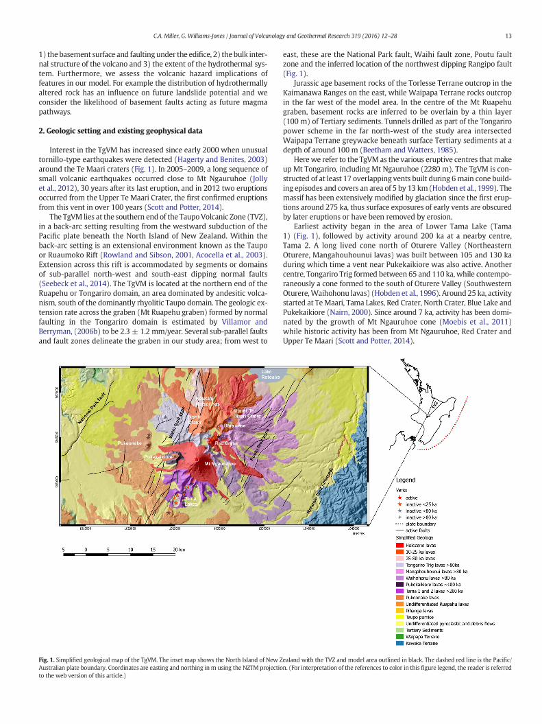
Interest in the TgVM has increased since early 2000 when unusualtornillo-type earthquakes were detected (Hagerty and Benites, 2003)around the Te Maari craters (Fig. 1). In 2005–2009, a long sequence ofsmall volcanic earthquakes occurred close to Mt Ngauruhoe (Jollyet al., 2012), 30 years after its last eruption, and in 2012 two eruptionsoccurred from the Upper Te Maari Crater, the first confirmed eruptionsfrom this vent in over 100 years (Scott and Potter, 2014).

The TgVM lies at the southern end of the TaupoVolcanic Zone (TVZ),in a back-arc setting resulting from the westward subduction of thePacific plate beneath the North Island of New Zealand. Within theback-arc setting is an extensional environment known as the Taupoor Ruaumoko Rift (Rowland and Sibson, 2001, Acocella et al., 2003).Extension across this rift is accommodated by segments or domainsof sub-parallel north-west and south-east dipping normal faults(Seebeck et al., 2014). The TgVM is located at the northern end of theRuapehu or Tongariro domain, an area dominated by andesitic volca-nism, south of the dominantly rhyolitic Taupo domain. The geologic ex-tension rate across the graben (Mt Ruapehu graben) formed by normalfaulting in the Tongariro domain is estimated by Villamor andBerryman, (2006b) to be 2.3 ± 1.2 mm/year. Several sub-parallel faultsand fault zones delineate the graben in our study area; from west to

Fig. 1. Simplified geological map of the TgVM. The inset map shows the North Island of New ZAustralian plate boundary. Coordinates are easting and northing in m using the NZTM projectioto the web version of this article.)

east, these are the National Park fault, Waihi fault zone, Poutu faultzone and the inferred location of the northwest dipping Rangipo fault(Fig. 1).

Jurassic age basement rocks of the Torlesse Terrane outcrop in theKaimanawa Ranges on the east, while Waipapa Terrane rocks outcropin the far west of the model area. In the centre of the Mt Ruapehugraben, basement rocks are inferred to be overlain by a thin layer(100 m) of Tertiary sediments. Tunnels drilled as part of the Tongariropower scheme in the far north-west of the study area intersectedWaipapa Terrane greywacke beneath surface Tertiary sediments at adepth of around 100 m (Beetham and Watters, 1985).

Here we refer to the TgVM as the various eruptive centres that makeup Mt Tongariro, including Mt Ngauruhoe (2280 m). The TgVM is con-structed of at least 17 overlapping vents built during 6main cone build-ing episodes and covers an area of 5 by 13 km (Hobden et al., 1999). Themassif has been extensively modified by glaciation since the first erup-tions around 275 ka, thus surface exposures of early vents are obscuredby later eruptions or have been removed by erosion.

Earliest activity began in the area of Lower Tama Lake (Tama1) (Fig. 1), followed by activity around 200 ka at a nearby centre,Tama 2. A long lived cone north of Oturere Valley (NortheasternOturere, Mangahouhounui lavas) was built between 105 and 130 kaduring which time a vent near Pukekaikiore was also active. Anothercentre, Tongariro Trig formed between 65 and 110 ka, while contempo-raneously a cone formed to the south of Oturere Valley (SouthwesternOturere,Waihohonu lavas) (Hobden et al., 1996). Around 25 ka, activitystarted at TeMaari, Tama Lakes, Red Crater, North Crater, Blue Lake andPukekaikiore (Nairn, 2000). Since around 7 ka, activity has been domi-nated by the growth of Mt Ngauruhoe cone (Moebis et al., 2011)while historic activity has been from Mt Ngauruhoe, Red Crater andUpper Te Maari (Scott and Potter, 2014).

ealand with the TVZ and model area outlined in black. The dashed red line is the Pacific/n. (For interpretation of the references to color in this figure legend, the reader is referred

14 C.A. Miller, G. Williams-Jones / Journal of Volcanology and Geothermal Research 319 (2016) 12–28

Flank collapse has punctuated cone building episodes, either trig-gered by eruptions (Lecointre et al., 2002), or triggering eruptions byrapidly de-pressurising the hydrothermal system (Jolly et al., 2014). Inboth cases, the active hydrothermal system played an important rolein mechanically weakening the rock prior to failure (Breard et al.,2014). Currently the largest surface hydrothermal features are at RedCrater, Ketetahi and Te Maari craters, although other mapped areas ofalteration suggest a long history of hydrothermal activity in many loca-tions on the massif. What is not documented from surface mapping ishow extensive alteration is within the massif.

2.1. Previous geophysical studies

Previous geophysical studies have imaged the structure, magmaticand hydrothermal systems of the TgVMat varying degrees of resolution.Zeng and Ingham (1993) undertook two dimensional modelling ofsparse gravity data along a profile south of Tama Lakes and suggestedthe presence of low density pyroclastic material overlying a dense base-ment.Walsh et al. (1998) summarised electrical resistivity data todelin-eate the extent of the hydrothermal system along a single profile; theyfound a shallow low resistivity layer, interpreted as geothermal conden-sate several hundred metres thick, overlying a vapour-dominated layerof unknown thickness. Rowlands et al. (2005) undertook a moderateresolution seismic tomography study and identified significant low ve-locity anomalies beneath Mts Ruapehu, Tongariro and Ngauruhoewhich they interpreted as remnant magma batches and thick pyroclas-tic material from various volcanic sources. Cassidy et al. (2009) pro-duced a more detailed 2D model across the Tama Lakes profile, fromnew gravity, aeromagnetic and magnetotelluric (MT) data. They alsomodelled the basement structure and inferred that the Waihi faultswere pathways for magma intrusion into the TgVM. Johnson et al.(2011) and Johnson and Savage (2012) used seismic anisotropy mea-surements tomap spatial and temporal changes in anisotropy; in partic-ular they found a strong change in anisotropy north of Mt Ngauruhoewhich they associated with the TgVM hydrothermal system. Hill et al.(2015) undertook a detailed 3D MT survey and found evidence forboth shallow and deep conductive zones, interpreted as magma ascentpathways and deeper storage zones. In particular, they found a narrow(1 km) vertical conductive zone under Mt Ngauruhoe interpreted torepresent the ascent path of magmatic fluids from a source at 4-12 kmdepth.

2.2. Physical property measurements

The TgVM consists of a variety of rock types including alternatinglayers of highly vesicular scoria and dense lavas, underlain by densemeta-sediments. To constrain the physical properties of different rockunits for modelling, we extracted a dataset of 176 samples from theGNS Science PetLab database (http://pet.gns.cri.nz) from rocks onand around the TgVM. Physical properties include wet and dry densityand magnetic susceptibility. We also incorporated physical propertymeasurements from several studies of individual vents of the TgVM;including Tongariro (Hackett, 1985), North Crater (Griffin, 2007), MtNgauruhoe, (Krippner, 2009; Sanders, 2010), and Blue Lake (Simons,2014), for a total of 288 measurements. For analysis purposes, we

Table 1Summary of physical properties for rock types within the TgVM. All volcanic includes all andes

Dry density Dry density Wet density

Mean (kg/m3) Stdev (kg/m3) Mean (kg/m3)

Andesite lava 2384 (n = 132) 302 2535 (n = 108)Pyroclastic 1591 (n = 143) 569 1931 (n = 143)All volcanic 1971 (n = 275) 607 2334 (n = 251)Greywacke 2706 (n = 31) 56 2727 (n = 30)Sandstone 2407 (n = 3) 6 2517 (n = 3)

grouped samples into four main rock types: Andesite lava, referring todense lavaflows; Pyroclastic, a range ofmaterial frompumice and scoriato denser welded agglutinates; Greywacke, referring to basementTorlesse and Waipapa Terrane rocks; and Sandstone, Tertiary sand-stones from the Taumarunui Formation.

For each rock type, we computed physical property histograms(Supplementary Material Fig. 3) with the mean and standard deviationfor each (Table 1). Wet densities better represent whole rock densitiesfor rocks that are below thewater table and aremore suitable for gravitymodelling. Depending on theporosity of the rock, dry vswet densities inthese samples can vary by as much as 340 kg/m3.

Magnetic susceptibilities of fresh volcanic rock samples range from0.001 to 0.04 SI, while basement greywacke rocks are only very weaklymagnetic (b0.001 SI) or non-magnetic (below detection limit). Huntand Mumme (1986) showed magnetisation intensities of young MtNgauruhoe lavas range from 0.7 to 49 A/m from unweathered samples.No samples of hydrothermally altered rock were available in the data-base and measurements of magnetic susceptibility in volcanic rocksmay be dominated by remnant magnetisation, so are only used as aguide.

3. Geophysical data acquisition and processing

Our study covers 504 km2within a rectangle 28 km× 18 km rangingin elevation from 600m to 2300m. This region encompasses all the lavaflows from the TgVM and includes basement rocks outcropping to theeast and west of the volcano.

3.1. Gravity survey design

We collected gravity data along radial traverses on foot, from thesummit of the volcano massif (~2200 m) to the tree line (~1100 m)where thick vegetation prevented further surveying. This results in a2–3 km wide region with no coverage from 1100 m to 700 m. Below700 m, surveying resumed along the roads at the base of the volcano.The area with no coverage consists mostly of distal lava flows and pyro-clastic deposits. Station spacing along the traverses is 500 m and tra-verses were located approximately 1 km apart; spacing reflects atrade-off between completing coverage of the entire volcano and reso-lution of structures in the volcano. At 500 m station spacing, Nyquisttheorem indicates wewill be able to resolve features with awavelengthof N1000mwhich is considered adequate for the size of the volcano, butwe would not be able to resolve small scale features such as individualfeeder dykes as observed at Red Crater (Wadsworth et al., 2015).However, we can resolve large scale fault offsets and bulk rock physicalproperty distributions related to different parts of the volcano andhydrothermal system. The station density across the survey area is0.8 stations/km2 which increases to 1.4 stations/km2 on the upperflanks of the volcano.

3.2. Gravity datasets

Our gravity dataset contains data from three sources. The oldestdata, sourced from the GNS Science New Zealand gravity stationdatabase (http://gns.cri.nz/Home/Products/Databases/New-Zealand-

ite lava and pyroclastic samples. Number of samples of each rock type is given by n.

Wet density Magnetic susceptibility Magnetic susceptibility

Stdev (kg/m3) Mean (SI) Stdev (SI)

205 0.022 (n = 94) 0.017267 0.009 (n = 46) 0.010364 0.017 (n = 140) 0.016456


Gravity-Station-Network), provides absolute gravity values referencedto the IGSN71 gravity datum (Morelli et al., 1974). These data providefar field, regional coverage to a distance of 40 km from the TgVM.Many of the 576 stations selected date from the 1960s, '70s and '80sandwere located with accuracies of 100m horizontally and N5m verti-cally. Repeat occupation of a subset of these stations during the currentsurvey reveals no systematic offset between current and old readingswith most stations being repeatable to within 0.2 mGal. As a controlon data quality, we excluded GNS Science data with measured eleva-tions that are grossly different (10s of m) from a 10 m Digital ElevationModel (DEM). These mostly occur in areas of steep terrain to the east ofthe study area where the poor horizontal positioning results in a largeelevation difference.

The second dataset comprises 66 stations on themassif from Cassidyand Locke (1995) and Cassidy et al. (2009). These data were locatedusing a mixture of barometry, precise levelling and differential GPS,hence height accuracies vary from ~5 m to b0.5 m.

The third dataset is newdatawe collected at 315 stations over 2 fieldcampaigns in 2014 and 2015. Vertical and horizontal positionswere de-termined using differential GNSS (using a Trimble Geoexplorer XH), op-erating in rapid static mode with 2min occupations and post processedwith Trimble Pathfinder Office software using nearby GeoNet CGPSstations as reference stations. The short baselines between rover andbase stations (b10 km) allows gravity stations to be located with verti-cal accuracies of better than 0.2 m.

To combine the data from the 3 surveys, we reoccupied the primarybase station from the Cassidy survey and tied it to our newly establishedlocal base station. Repeatmeasurement of a selection of the Cassidy sta-tions showed values agreed within 0.12 mGal. Finally, we tied our localbase station back to the National Park reference station (GNS station ID96), so that both our and the Cassidy stationswere assigned an absolutegravity value, consistent with the GNS dataset.

3.3. Gravity data reduction and errors

We corrected the rawdata from the 2014 and 2015 surveys for Earthtide, ocean loading and drift (e.g. Battaglia et al., 2012) to produce datarelative to our local base. Average base station loop closure errors afterEarth tide and ocean loading are accounted for are 0.02 ± 0.03 mGal.We applied a correction scheme following that outlined in Hinze et al.(2005), across all generations of data, to compute a consistent dataset.Details of the correction scheme are in supplementary materials.

Estimating the overall error in gravity values from closure, height,positioning and terrain errors gives a RMS value of 0.070 mGal for the2014 and 2015 surveys. The Cassidy survey data has errors from 0.1 to1 mGal, while errors from the GNS Science dataset are up to ~1 mGal,mostly due to the poor accuracy of the height determination.

One of the most important choices in gravity data reduction is theselection of the reduction density applied to the Bouguer and terraincorrections. The shape and amplitude of the resulting complete Bougueranomaly can vary with choice of reduction density which directly influ-ences the resulting models. Methods such as Nettleton (1939) andParasnis (1966) or their derivatives (Gottsmann et al., 2008), are oftennot valid in heterogeneous volcanic rock environments so we use ourphysical property dataset instead. See supplementary materials for fur-ther discussion on the calculation of correction density from gravitymeasurements. We chose the mean volcanic rock wet density value of2334 kg/m3 (rounded down to 2300 kg/m3), to represent the bulk den-sity of the volcanomassif, for computing the complete Bouguer anoma-ly. This density is valid for the mass above the reduction datum, i.e., the

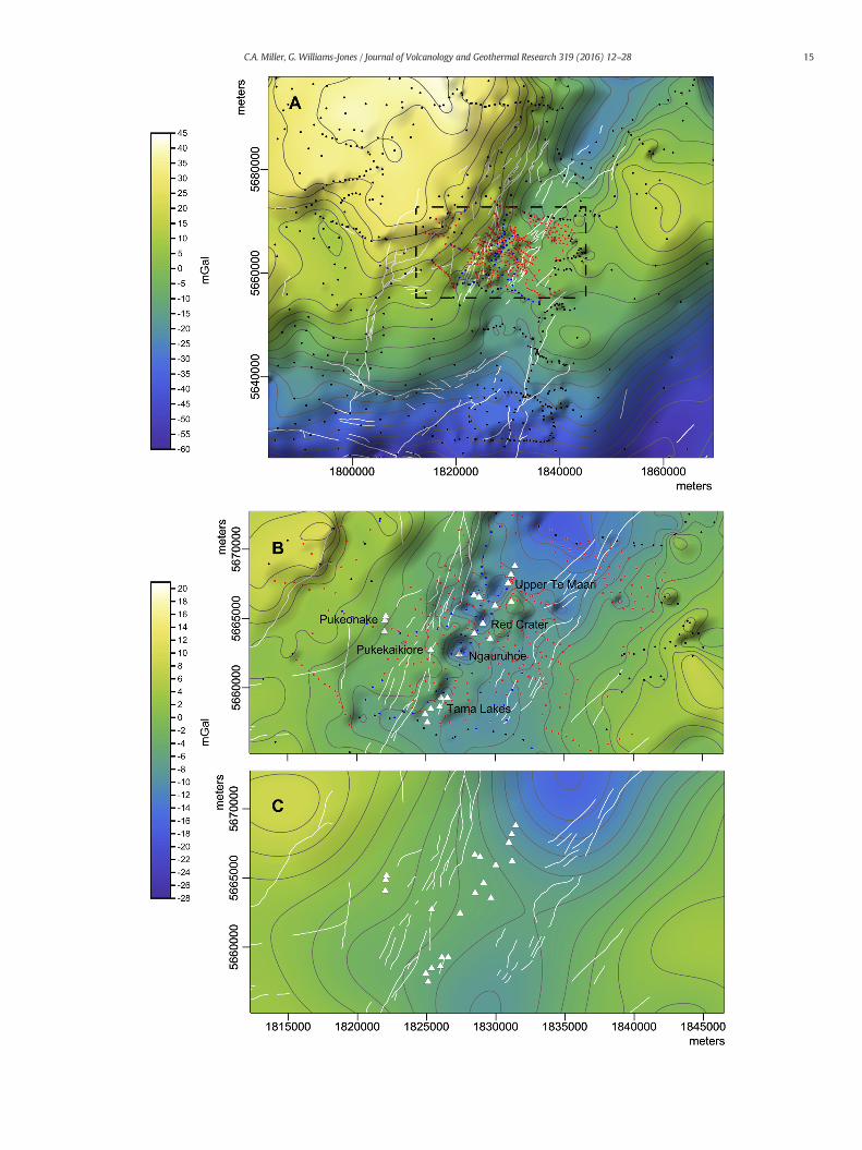
Fig. 2.Complete Bouguer anomaly data for A) regional area aroundMt Tongariro, contour intervdots are GNS Science stations, blue dots are Cassidy stations, red dots are stations collected incontour interval 2 mGal. Vent locations are shown in white triangles and stations as for part AShown in all figures are the active faults (white lines). Coordinates are easting and northing inlegend, the reader is referred to the web version of this article.)

ellipsoid. Our study area contains a wide variety of volcanic and base-ment rock types above this datum, so finding a single density suitablefor all rock types is not possible and may have resulted in parts of thedataset being over or under corrected. Howeverwe consider our chosencorrection density to be in themiddle of the range of all rock types, thusany error caused by over or underestimation of the correction densityshould be evenly distributed around the chosen value and not overlybias the results.

3.4. Complete Bouguer anomaly

We computed the complete Bouguer anomaly (CBA) on the datasetof 957 stations, covering an area of 70 kmby 80 km in order to accurate-ly determine the regional gravity in the area of interest around thevolcanoes (Fig. 2A). The regional CBA ranges from +41 mGal in thenorthwest to−54mGal in the south and broadly consists of two gravityhighs to the northwest and east. These highs correlate with mappedareas of outcropping basement Torlesse Terrane in the east and theWaipapa Terrane in the west (Fig. 1). Between these highs is a broadgravity low defining the width of the Taupo Volcanic Zone. The TgVMis situated at a local maximum in this gravity low which decreasesfurther to the north-east and also to the south, towards Mt Ruapehu.The strike of the gravity signal changes from NE–SW to E–W just tothe south of Mt Ruapehu, representing the termination of the TVZ.

In the modelling area (dashed box in Fig. 2A), the CBA shows abroad, asymmetric ‘U-shaped’ trend, descending steeply from a gravityhigh (28 mGal) in the north-west to a broad low (−4 mGal) and thenincreasing gradually to another high (12 mGal) in the east (Fig. 2B).The TgVM is located on the west side of the gravity low, and ischaracterised by short wavelength anomalies with localised maximaand minima (±6 mGal). Local minima are associated with thecones of Mt Ngauruhoe, Red Crater, Mt Tongariro summit and TeMaari as well as with the Upper Tama Lake crater. Local maxima arelocated in the Oturere Valley to the east of Red Crater and to the eastof Blue Lake. A small gravity high is also located in the MangatepopoValley.

Modelling requires removal of a regional field that creates a longwavelength gradient across the anomalymap reflecting the broad crust-al structure relating to the TVZ and the subduction zone to the east. Zengand Ingham (1993) and Cassidy et al. (2009) fit the regional field in theTongariro area using a third order polynomial calculated from stationslocated on outcropping basement rocks. The use of a third order polyno-mial is common in gravity studies throughout the TVZ (e.g., Stern, 1979;Stagpoole and Bibby, 1999; Caratori Tontini et al., 2015).We remove thesame regional field from our data and the resulting residual anomalymap is shown in Fig. 2B.

3.5. Aeromagnetic data acquisition and processing

Approximately 510 line kilometres of aeromagnetic data were ac-quired in February 1995, along 19 flight lines, at a nominal 500 m spac-ing, of which only the southernmost line is published in Cassidy et al.(2009). A proton precession magnetometer was towed 100 m behinda Cessna fixed-wing aircraft and data were acquired at 2 s intervalswhich for an average flight speed of 100 knots resulted in 1 sample ap-proximately every 100 m. The survey was flown at a constant altitudeconfiguration with a mean altitude of 2450 m, although turbulencemeant that flight altitude could vary by as much as 100 m above orbelow the mean, along each line. Flight lines were oriented NW–SEperpendicular to the main strike of the TVZ. A single tie line was flown

al 5mGal. Thedetailed 28×18 kmmodel area is shown in the blackdashed rectangle. Blackthis study. B) The residual CBA in the model area after removal of a 3rd order polynomial,. C) The residual CBA low pass filtered to 10,000 m wavelength, contour interval 2 mGal.m using the NZTM projection. (For interpretation of the references to color in this figure

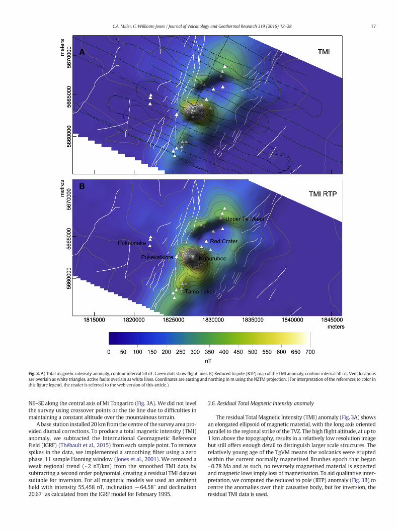
Fig. 3. A) Total magnetic intensity anomaly, contour interval 50 nT. Green dots show flight lines. B) Reduced to pole (RTP) map of the TMI anomaly, contour interval 50 nT. Vent locationsare overlain as white triangles, active faults overlain as white lines. Coordinates are easting and northing in m using the NZTM projection. (For interpretation of the references to color inthis figure legend, the reader is referred to the web version of this article.)


NE–SE along the central axis of Mt Tongariro (Fig. 3A). We did not levelthe survey using crossover points or the tie line due to difficulties inmaintaining a constant altitude over the mountainous terrain.

A base station installed 20 km from the centre of the survey area pro-vided diurnal corrections. To produce a total magnetic intensity (TMI)anomaly, we subtracted the International Geomagnetic ReferenceField (IGRF) (Thébault et al., 2015) from each sample point. To removespikes in the data, we implemented a smoothing filter using a zerophase, 11 sample Hanning window (Jones et al., 2001). We removed aweak regional trend (~2 nT/km) from the smoothed TMI data bysubtracting a second order polynomial, creating a residual TMI datasetsuitable for inversion. For all magnetic models we used an ambientfield with intensity 55,458 nT, inclination −64.58° and declination20.67° as calculated from the IGRF model for February 1995.

3.6. Residual Total Magnetic Intensity anomaly

The residual TotalMagnetic Intensity (TMI) anomaly (Fig. 3A) showsan elongated ellipsoid of magnetic material, with the long axis orientedparallel to the regional strike of the TVZ. The high flight altitude, at up to1 km above the topography, results in a relatively low resolution imagebut still offers enough detail to distinguish larger scale structures. Therelatively young age of the TgVM means the volcanics were eruptedwithin the current normally magnetised Brunhes epoch that began~0.78 Ma and as such, no reversely magnetised material is expectedandmagnetic lows imply loss of magnetisation. To aid qualitative inter-pretation, we computed the reduced to pole (RTP) anomaly (Fig. 3B) tocentre the anomalies over their causative body, but for inversion, theresidual TMI data is used.

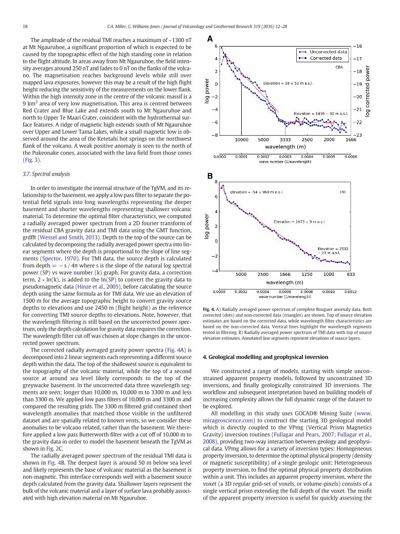
Fig. 4. A) Radially averaged power spectrum of complete Bouguer anomaly data. Bothcorrected (dots) and non-corrected data (triangles) are shown. Top of source elevationestimates are based on the corrected data, while wavelength filter characteristics arebased on the non-corrected data. Vertical lines highlight the wavelength segmentstested in filtering. B) Radially averaged power spectrum of TMI data with top of sourceelevation estimates. Annotated line segments represent elevations of source layers.


The amplitude of the residual TMI reaches a maximum of ~1300 nTat Mt Ngauruhoe, a significant proportion of which is expected to becaused by the topographic effect of the high standing cone in relationto the flight altitude. In areas away fromMt Ngauruhoe, the field inten-sity averages around 250 nT and fades to 0 nT on the flanks of the volca-no. The magnetisation reaches background levels while still overmapped lava exposures, however this may be a result of the high flightheight reducing the sensitivity of themeasurements on the lower flank.Within the high intensity zone in the centre of the volcanic massif is a9 km2 area of very low magnetisation. This area is centred betweenRed Crater and Blue Lake and extends south to Mt Ngauruhoe andnorth to Upper Te Maari Crater, coincident with the hydrothermal sur-face features. A ridge of magnetic high extends south of Mt Ngauruhoeover Upper and Lower Tama Lakes, while a small magnetic low is ob-served around the area of the Ketetahi hot springs on the northwestflank of the volcano. A weak positive anomaly is seen to the north ofthe Pukeonake cones, associated with the lava field from those cones(Fig. 3).

3.7. Spectral analysis

In order to investigate the internal structure of the TgVM, and its re-lationship to the basement, we apply a lowpass filter to separate the po-tential field signals into long wavelengths representing the deeperbasement and shorter wavelengths representing shallower volcanicmaterial. To determine the optimal filter characteristics, we computeda radially averaged power spectrum from a 2D fourier transform ofthe residual CBA gravity data and TMI data using the GMT function,grdfft (Wessel and Smith, 2013). Depth to the top of the source can becalculated by decomposing the radially averaged power spectra into lin-ear segments where the depth is proportional to the slope of line seg-ments (Spector, 1970). For TMI data, the source depth is calculatedfrom depth = −s / 4π where s is the slope of the natural log spectralpower (SP) vs wave number (k) graph. For gravity data, a correctionterm, 2 ∗ ln(k), is added to the ln(SP) to convert the gravity data topseudomagnetic data (Hinze et al., 2005), before calculating the sourcedepth using the same formula as for TMI data. We use an elevation of1500 m for the average topographic height to convert gravity sourcedepths to elevations and use 2450 m (flight height) as the referencefor converting TMI source depths to elevations. Note, however, thatthe wavelength filtering is still based on the uncorrected power spec-trum, only the depth calculation for gravity data requires the correction.The wavelength filter cut off was chosen at slope changes in the uncor-rected power spectrum.

The corrected radially averaged gravity power spectra (Fig. 4A) isdecomposed into 2 linear segments each representing a different sourcedepth within the data. The top of the shallowest source is equivalent tothe topography of the volcanic material, while the top of a secondsource at around sea level likely corresponds to the top of thegreywacke basement. In the uncorrected data three wavelength seg-ments are seen; longer than 10,000 m, 10,000 m to 3300 m and lessthan 3300 m. We applied low pass filters of 10,000 m and 3300 m andcompared the resulting grids. The 3300 m filtered grid contained shortwavelength anomalies that matched those visible in the unfiltereddataset and are spatially related to known vents, so we consider theseanomalies to be volcano related, rather than the basement. We there-fore applied a low pass Butterworth filter with a cut off of 10,000 m tothe gravity data in order to model the basement beneath the TgVM asshown in Fig. 2C.

The radially averaged power spectrum of the residual TMI data isshown in Fig. 4B. The deepest layer is around 50 m below sea leveland likely represents the base of volcanic material as the basement isnon-magnetic. This interface corresponds well with a basement sourcedepth calculated from the gravity data. Shallower layers represent thebulk of the volcanic material and a layer of surface lava probably associ-ated with high elevation material on Mt Ngauruhoe.

4. Geological modelling and geophysical inversion

We constructed a range of models, starting with simple uncon-strained apparent property models, followed by unconstrained 3Dinversions, and finally geologically constrained 3D inversions. Theworkflow and subsequent interpretation based on building models ofincreasing complexity allows the full dynamic range of the dataset tobe explored.

All modelling in this study uses GOCAD® Mining Suite (www.mirageoscience.com) to construct the starting 3D geological modelwhich is directly coupled to the VPmg (Vertical Prism MagneticsGravity) inversion routines (Fullagar and Pears, 2007; Fullagar et al.,2008), providing two-way interaction between geology and geophysi-cal data. VPmg allows for a variety of inversion types: Homogeneousproperty inversion, to determine the optimal physical property (densityor magnetic susceptibility) of a single geologic unit; Heterogeneousproperty inversion, to find the optimal physical property distributionwithin a unit. This includes an apparent property inversion, where thevoxet (a 3D regular grid-set of voxels, or volume-pixels) consists of asingle vertical prism extending the full depth of the voxet. The misfitof the apparent property inversion is useful for quickly assessing the


degree of three dimensionality in the data. Finally, geometry inversionof geological contacts optimise the shape of a unit while its physicalproperty remains constant. Each type of inversion can be applied se-quentially and in combination. VPmg models the subsurface as a set ofvertical rectangular prisms whose top surface matches the topography.Internally, the prisms are divided into cells with arbitrary verticaldimension. Cell subdivisions can be based on geologic units and eachunit can be assigned homogeneous or heterogeneous physical proper-ties. Heterogeneous units can be inverted in a smooth sense via leastsquares or stochastically. In stochastic inversion, random perturbationsare chosen for each cell of each geologic unit. The size of the randomperturbations is governed by the a priori defined property distributionand limited to three standard deviations from the mean propertyvalue of the unit being inverted. The perturbation is accepted if it re-duces the chi-squared misfit, and is rejected otherwise (Fullagar andPears, 2007). The RMS misfit (mGal) is computed and recorded, where

RMS ¼ffiffiffiffiffiffiffiffiffiffiffiffiffiffiffiffiffiffiffiffiffiffiffiffiffiffiffiffiffiffiffiffiffiffiffiffiffiffi1=N

XNn¼1

On−Cnð Þ2vuut ð1Þ

where N is the number of data, On is the measured data and Cn thecalculated model response.

Mathematical details of the inversion method are provided insupplementary material.

4.1. Model initialisation

Voxet cell sizes are 250 m (half gravity station spacing) in the eastand north axes and 100m in the vertical (depth) axis. VPmgmathemat-ically extends the model volume to 25 km depth to ensure completemodelling of the data at all wavelengths. The voxet is then embeddedin a halfspace so that the model does not terminate abruptly, reducingedge effects. The physical property of the halfspace is optimised by theinversion routine.

We gridded the observed gravity and magnetic data at a 250 m cellsize to ensure that each vertical prism in the voxet is associated with 1data point located in the centre of the prism. VPmg requires the inputof a topographic surface as the top surface of the model, so that thetopography is modelled directly. This was constructed using a pointdataset from an 8 m DEM (down sampled to 24 m) as constraints forfitting a smooth surface using the DSI interpolator in GOCAD. Theresulting surface consists of a mesh of equilateral triangles with~100 m sides. This topographic surface is then down sampled to the250 m voxet for modelling.

We beginwith a simple two layer case, consisting of a basement unitand a cover unit of volcanics; the complex geological history of theTgVM makes constructing a more detailed model highly subjective. In-stead, we use the inversion process to discover detail within the subsur-face and focus on building geological constraints into the model fromkilometre scale features.

To construct the basement surface, we imported into GOCAD shapefiles of surface fault traces from the GNS Science New Zealand ActiveFault Database and outlines of geological units from GNS ScienceHawke's Bay QMAP (Lee et al., 2011). We used the mapped contactsto accurately define the basement–volcanics boundary in our model.We have not explicitly modelled the thin (~100 m) overlying layer ofTertiary sediments as they have a similar density to the average volcanicrock density and distinguishing the twowithout other constraints is dif-ficult. Using the DEM and the basement geology contact curves, wewarped a flat starting surface to the shape of the outcropping basementtopography. We then overlaid the surface fault traces of the NationalPark, Waihi, Poutu and Rangipo fault zones. These fault zones aremade from numerous sub-parallel strands and modelling each individ-ual strand is outside the resolution of our gravity data. As such, only themajor fault strands were included. We assigned initial offsets to these

faults based on the model of Cassidy et al. (2009) and consistent withthe mapped continuation of the faults outside the study area byVillamor and Berryman (2006b).We thenwarped the basement surfaceto fit the fault offsets. As a sensitivity test of our model to the startinggeometry, we also created a flat basement surface that only includedthe outcropping basement, i.e., with no fault steps in it.

5. Results

We began our exploration of the data by first performing apparentproperty inversions to determine the broad lateral distribution of phys-ical properties.We then performed anunconstrained 3D inversion to in-vestigate the approximate vertical extent of anomalous features. Theseresults (see supplementary material) highlight the necessity to betterconstrain the depth to the basement interface which from our knowl-edge of the geology and petrophysical contrasts suggests should be asharp interface.

5.1. 3D geologically constrained density inversion

To begin the geologically constrained model, we first used a geome-try inversion to adjust the shape of the starting basement surface to fitthe low pass filtered gravity data. In the geometry inversion, the base-ment density contrast is fixed at 400 kg/m3 (to represent an absolutevalue of 2700 kg/m3 matching our petrophysical data) and the top ofthe basement in each voxet cell is allowed to vary vertically. Theresulting RMSmisfit for thismodel is 1.7mGal. The areas of worstmisfitare associated with older GNS Science stations that may have errors upto 1mGal. To test for any density variations in the basement whichmayimprove the fit of the model, we performed a second inversion on thestarting basement surface, comprising a combined geometry and het-erogeneous property inversion. In this approach, alternating steps of asingle heterogeneous density inversion iteration, followed by a singlegeometry inversion iteration are run to produce a model that accountsfor both the geometry and density contrasts within the basement. Thisimproved the misfit RMS to 0.75 mGal.

With the shape of the basement now constrained, we model thecover unit using a heterogeneous density inversion. In this model, thebest fit basement geometry and physical property distribution, as de-scribed above, is fixed and the initially homogeneous cover unit is con-verted to a heterogeneous unit. We then perform both a conventionalinversion and a stochastic inversion in the cover unit using the unfil-tered, full wavelength, gravity data. In this way we are fitting theremainder of the gravity signal, not accounted for by the basementmodel, by density variations in the cover unit. The final conventionalinversionmodel of the full dataset has anRMS of 0.9mGalwhile the sto-chastic inversion produces a model with RMS of 0.93 mGal, with thehighestmisfits associatedwith poorer quality gravity stations. This mis-fit is due to the combination of the fit of the basement surface plus themisfit due to the heterogeneous cover model. When the basement mis-fit is subtracted, the misfit due to the cover unit alone is 0.15 mGal.

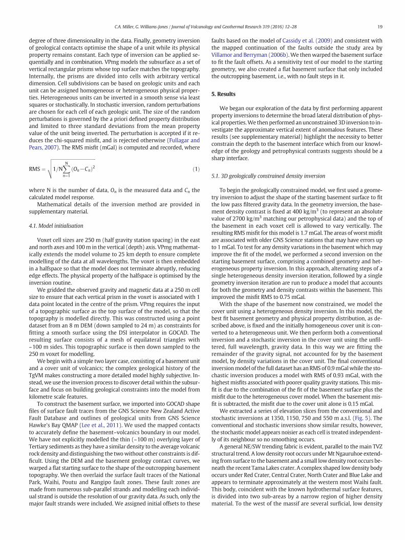
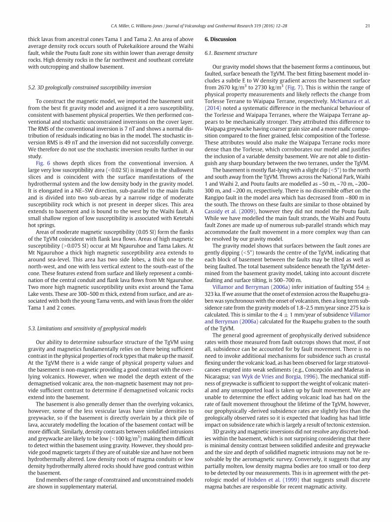
We extracted a series of elevation slices from the conventional andstochastic inversions at 1350, 1150, 750 and 550 m a.s.l. (Fig. 5). Theconventional and stochastic inversions show similar results, however,the stochasticmodel appears noisier as each cell is treated independent-ly of its neighbour so no smoothing occurs.

A general NE/SW trending fabric is evident, parallel to themain TVZstructural trend. A lowdensity root occurs underMtNgauruhoe extend-ing from surface to thebasement and a small lowdensity root occurs be-neath the recent Tama Lakes crater. A complex shaped low density bodyoccurs under Red Crater, Central Crater, North Crater and Blue Lake andappears to terminate approximately at the western most Waihi fault.This body, coincident with the known hydrothermal surface features,is divided into two sub-areas by a narrow region of higher densitymaterial. To the west of the massif are several surficial, low density

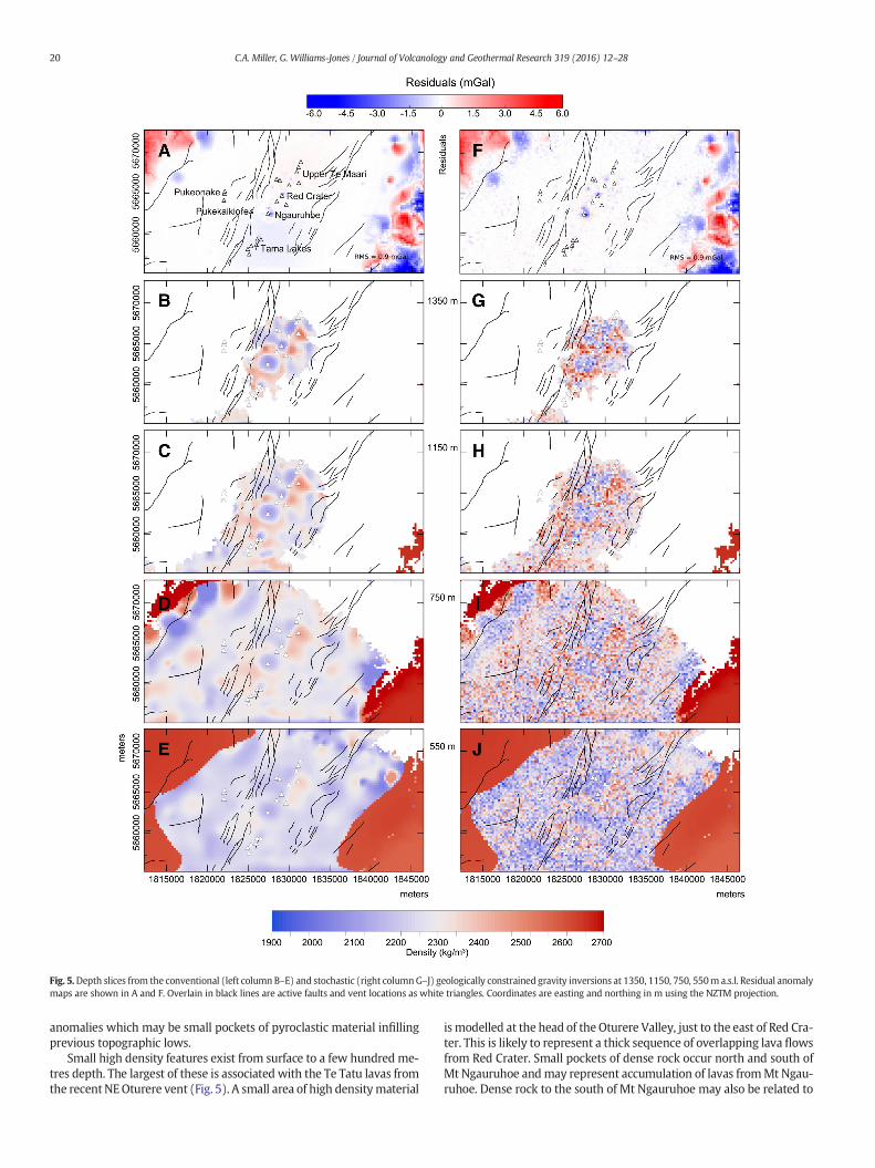
Fig. 5.Depth slices from the conventional (left column B–E) and stochastic (right columnG–J) geologically constrained gravity inversions at 1350, 1150, 750, 550m a.s.l. Residual anomalymaps are shown in A and F. Overlain in black lines are active faults and vent locations as white triangles. Coordinates are easting and northing in m using the NZTM projection.


anomalies which may be small pockets of pyroclastic material infillingprevious topographic lows.

Small high density features exist from surface to a few hundred me-tres depth. The largest of these is associated with the Te Tatu lavas fromthe recentNEOturere vent (Fig. 5). A small area of high densitymaterial

is modelled at the head of the Oturere Valley, just to the east of Red Cra-ter. This is likely to represent a thick sequence of overlapping lava flowsfrom Red Crater. Small pockets of dense rock occur north and south ofMt Ngauruhoe andmay represent accumulation of lavas fromMt Ngau-ruhoe. Dense rock to the south of Mt Ngauruhoe may also be related to


thick lavas from ancestral cones Tama 1 and Tama 2. An area of aboveaverage density rock occurs south of Pukekaikiore around the Waihifault, while the Poutu fault zone sits within lower than average densityrocks. High density rocks in the far northwest and southeast correlatewith outcropping and shallow basement.

5.2. 3D geologically constrained susceptibility inversion

To construct the magnetic model, we imported the basement unitfrom the best fit gravity model and assigned it a zero susceptibility,consistent with basement physical properties. We then performed con-ventional and stochastic unconstrained inversions on the cover layer.The RMS of the conventional inversion is 7 nT and shows a normal dis-tribution of residuals indicating no bias in the model. The stochastic in-version RMS is 49 nT and the inversion did not successfully converge.We therefore do not use the stochastic inversion results further in ourstudy.

Fig. 6 shows depth slices from the conventional inversion. Alarge very low susceptibility area (b0.02 SI) is imaged in the shallowestslices and is coincident with the surface manifestations of thehydrothermal system and the low density body in the gravity model.It is elongated in a NE–SW direction, sub-parallel to the main faultsand is divided into two sub-areas by a narrow ridge of moderatesusceptibility rock which is not present in deeper slices. This areaextends to basement and is bound to the west by the Waihi fault. Asmall shallow region of low susceptibility is associated with Ketetahihot springs.

Areas of moderate magnetic susceptibility (0.05 SI) form the flanksof the TgVM coincident with flank lava flows. Areas of high magneticsusceptibility (N0.075 SI) occur at Mt Ngauruhoe and Tama Lakes. AtMt Ngauruhoe a thick high magnetic susceptibility area extends toaround sea-level. This area has two side lobes, a thick one to thenorth-west, and one with less vertical extent to the south-east of thecone. These features extend from surface and likely represent a combi-nation of the central conduit and flank lava flows from Mt Ngauruhoe.Two more high magnetic susceptibility units exist around the TamaLake vents. These are 300–500m thick, extend from surface, and are as-sociatedwith both the young Tama vents, andwith lavas from the olderTama 1 and 2 cones.

5.3. Limitations and sensitivity of geophysical models

Our ability to determine subsurface structure of the TgVM usinggravity and magnetics fundamentally relies on there being sufficientcontrast in the physical properties of rock types thatmakeup themassif.At the TgVM there is a wide range of physical property values andthe basement is non-magnetic providing a good contrast with the over-lying volcanics. However, when we model the depth extent of thedemagnetised volcanic area, the non-magnetic basement may not pro-vide sufficient contrast to determine if demagnetised volcanic rocksextend into the basement.

The basement is also generally denser than the overlying volcanics,however, some of the less vesicular lavas have similar densities togreywacke, so if the basement is directly overlain by a thick pile oflava, accurately modelling the location of the basement contact will bemore difficult. Similarly, density contrasts between solidified intrusionsand greywacke are likely to be low (b100 kg/m3) making them difficultto detect within the basement using gravity. However, they should pro-vide goodmagnetic targets if they are of suitable size and have not beenhydrothermally altered. Low density roots of magma conduits or lowdensity hydrothermally altered rocks should have good contrast withinthe basement.

Endmembers of the range of constrained and unconstrainedmodelsare shown in supplementary material.

6. Discussion

6.1. Basement structure

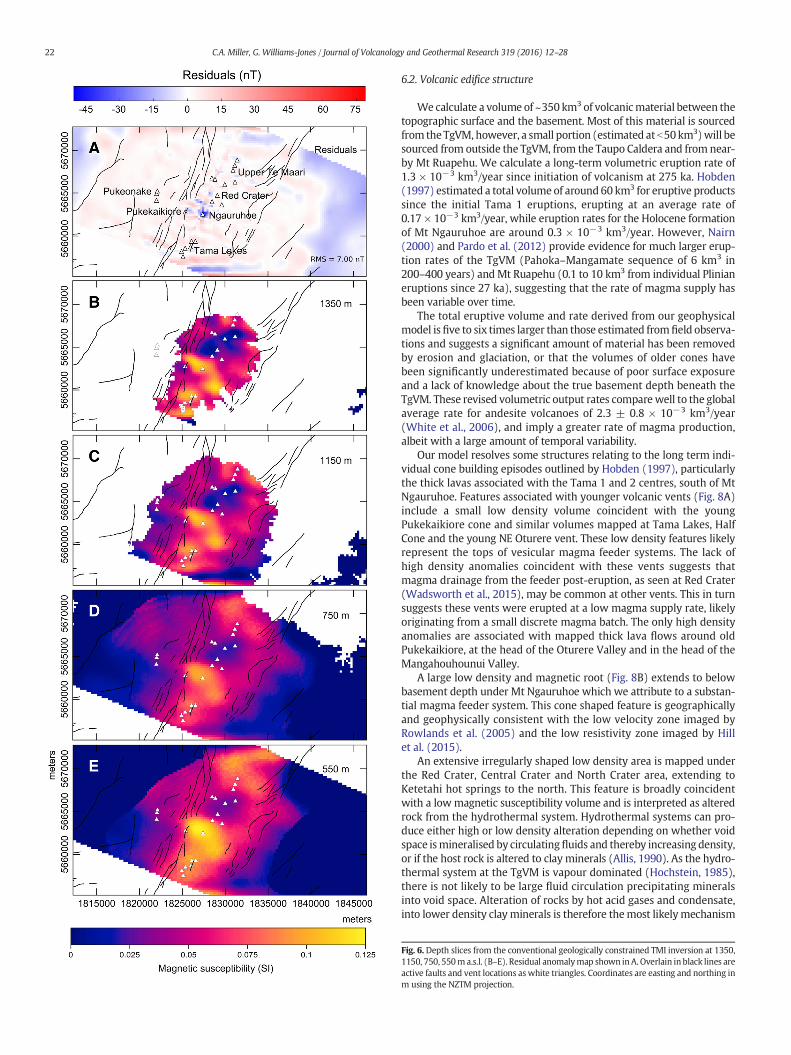
Our gravity model shows that the basement forms a continuous, butfaulted, surface beneath the TgVM. The best fitting basement model in-cludes a subtle E to W density gradient across the basement surfacefrom 2670 kg/m3 to 2730 kg/m3 (Fig. 7). This is within the range ofphysical property measurements and likely reflects the change fromTorlesse Terrane to Waipapa Terrane, respectively. McNamara et al.(2014) noted a systematic difference in the mechanical behaviour ofthe Torlesse and Waipapa Terranes, where the Waipapa Terrane ap-pears to be mechanically stronger. They attributed this difference toWaipapa greywacke having coarser grain size and amoremafic compo-sition compared to the finer grained, felsic composition of the Torlesse.These attributes would also make the Waipapa Terrane rocks moredense than the Torlesse, which corroborates our model and justifiesthe inclusion of a variable density basement. We are not able to distin-guish any sharp boundary between the two terranes, under the TgVM.

The basement ismostly flat-lyingwith a slight dip (b5°) to the northand south away from the TgVM. Throws across the National Park,Waihi1 and Waihi 2, and Poutu faults are modelled as ~50 m, ~70 m, ~200–300 m, and ~200 m, respectively. There is no discernible offset on theRangipo fault in the model area which has decreased from ~800 m inthe south. The throws on these faults are similar to those obtained byCassidy et al. (2009), however they did not model the Poutu fault.While we have modelled the main fault strands, the Waihi and Poutufault Zones are made up of numerous sub-parallel strands which mayaccommodate the fault movement in a more complex way than canbe resolved by our gravity model.

The gravity model shows that surfaces between the fault zones aregently dipping (b5°) towards the centre of the TgVM, indicating thateach block of basement between the faults may be tilted as well asbeing faulted. The total basement subsidence beneath the TgVM deter-mined from the basement gravity model, taking into account discretefaulting and surface tilting, is 500–700 m.

Villamor and Berryman (2006a) infer initiation of faulting 554 ±323 ka. If we assume that the onset of extension across the Ruapehu gra-benwas synchronouswith the onset of volcanism, then a long termsub-sidence rate from the gravitymodels of 1.8–2.5mm/year since 275 ka iscalculated. This is similar to the 4 ± 1 mm/year of subsidence Villamorand Berryman (2006a) calculated for the Ruapehu graben to the southof the TgVM.

The general good agreement of geophysically derived subsidencerates with those measured from fault outcrops shows that most, if notall, subsidence can be accounted for by fault movement. There is noneed to invoke additional mechanisms for subsidence such as crustalflexing under the volcanic load, as has been observed for large stratovol-canoes erupted into weak sediments (e.g., Concepción and Maderas inNicaragua; van Wyk de Vries and Borgia, 1996). The mechanical stiff-ness of greywacke is sufficient to support theweight of volcanic materi-al and any unsupported load is taken up by fault movement. We areunable to determine the effect adding volcanic load has had on therate of fault movement throughout the lifetime of the TgVM, however,our geophysically -derived subsidence rates are slightly less than thegeologically observed rates so it is expected that loading has had littleimpact on subsidence ratewhich is largely a result of tectonic extension.

3D gravity andmagnetic inversions did not resolve any discrete bod-ies within the basement, which is not surprising considering that thereis minimal density contrast between solidified andesite and greywackeand the size and depth of solidified magnetic intrusions may not be re-solvable by the aeromagnetic survey. Conversely, it suggests that anypartially molten, low density magma bodies are too small or too deepto be detected by our measurements. This is in agreement with the pet-rologic model of Hobden et al. (1999) that suggests small discretemagma batches are responsible for recent magmatic activity.


6.2. Volcanic edifice structure

Wecalculate a volume of ~350 km3 of volcanicmaterial between thetopographic surface and the basement. Most of this material is sourcedfrom theTgVM, however, a small portion (estimated atb50km3)will besourced from outside the TgVM, from the Taupo Caldera and from near-by Mt Ruapehu. We calculate a long-term volumetric eruption rate of1.3 × 10−3 km3/year since initiation of volcanism at 275 ka. Hobden(1997) estimated a total volume of around 60 km3 for eruptive productssince the initial Tama 1 eruptions, erupting at an average rate of0.17 × 10−3 km3/year, while eruption rates for the Holocene formationof Mt Ngauruhoe are around 0.3 × 10−3 km3/year. However, Nairn(2000) and Pardo et al. (2012) provide evidence for much larger erup-tion rates of the TgVM (Pahoka–Mangamate sequence of 6 km3 in200–400 years) and Mt Ruapehu (0.1 to 10 km3 from individual Plinianeruptions since 27 ka), suggesting that the rate of magma supply hasbeen variable over time.

The total eruptive volume and rate derived from our geophysicalmodel isfive to six times larger than those estimated from field observa-tions and suggests a significant amount of material has been removedby erosion and glaciation, or that the volumes of older cones havebeen significantly underestimated because of poor surface exposureand a lack of knowledge about the true basement depth beneath theTgVM. These revised volumetric output rates comparewell to the globalaverage rate for andesite volcanoes of 2.3 ± 0.8 × 10−3 km3/year(White et al., 2006), and imply a greater rate of magma production,albeit with a large amount of temporal variability.

Our model resolves some structures relating to the long term indi-vidual cone building episodes outlined by Hobden (1997), particularlythe thick lavas associated with the Tama 1 and 2 centres, south of MtNgauruhoe. Features associated with younger volcanic vents (Fig. 8A)include a small low density volume coincident with the youngPukekaikiore cone and similar volumes mapped at Tama Lakes, HalfCone and the young NE Oturere vent. These low density features likelyrepresent the tops of vesicular magma feeder systems. The lack ofhigh density anomalies coincident with these vents suggests thatmagma drainage from the feeder post-eruption, as seen at Red Crater(Wadsworth et al., 2015), may be common at other vents. This in turnsuggests these vents were erupted at a low magma supply rate, likelyoriginating from a small discrete magma batch. The only high densityanomalies are associated with mapped thick lava flows around oldPukekaikiore, at the head of the Oturere Valley and in the head of theMangahouhounui Valley.

A large low density and magnetic root (Fig. 8B) extends to belowbasement depth under Mt Ngauruhoe which we attribute to a substan-tial magma feeder system. This cone shaped feature is geographicallyand geophysically consistent with the low velocity zone imaged byRowlands et al. (2005) and the low resistivity zone imaged by Hillet al. (2015).

An extensive irregularly shaped low density area is mapped underthe Red Crater, Central Crater and North Crater area, extending toKetetahi hot springs to the north. This feature is broadly coincidentwith a lowmagnetic susceptibility volume and is interpreted as alteredrock from the hydrothermal system. Hydrothermal systems can pro-duce either high or low density alteration depending on whether voidspace ismineralised by circulatingfluids and thereby increasing density,or if the host rock is altered to clay minerals (Allis, 1990). As the hydro-thermal system at the TgVM is vapour dominated (Hochstein, 1985),there is not likely to be large fluid circulation precipitating mineralsinto void space. Alteration of rocks by hot acid gases and condensate,into lower density clay minerals is therefore themost likelymechanism

Fig. 6. Depth slices from the conventional geologically constrained TMI inversion at 1350,1150, 750, 550m a.s.l. (B–E). Residual anomalymap shown inA. Overlain in black lines areactive faults and vent locations as white triangles. Coordinates are easting and northing inm using the NZTM projection.

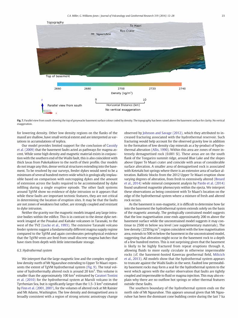
Fig. 7.Parallel view from south showing the top of greywacke basement surface colour coded bydensity. The topography has been raised above the basement surface for clarity. No verticalexaggeration.


for lowering density. Other low density regions on the flanks of themassif are shallow, have small vertical extent and are interpreted as var-iations in accumulations of tephra.

Our model provides limited support for the conclusion of Cassidyet al. (2009) that the basement faults acted as pathways for magma as-cent. While some high density andmagnetic material exists in conjunc-tionwith the southern end of theWaihi fault, this is also coincidentwiththick lavas from Pukekaikiore to the north of their profile. Our modelsdo not image any thin, dense vertical structures extending into thebase-ment. To be resolved by our surveys, feeder dykes would need to be aminimumof several hundredmetreswidewhich is geologically implau-sible based on comparison with outcropping dykes and the amountof extension across the faults required to be accommodated by dykeinfilling during a single eruptive episode. The other fault systemsaround TgVM show no evidence of dyke intrusion so it appears thatwhile these faults are important tectonic features, they are not criticalin determining the location of eruption sites. It may be that the faultsare not zones of weakness but rather, are strongly coupled and resistantto dyke intrusion.

Neither the gravity nor themagnetic models imaged any large intru-sive bodies within the edifice. This is in contrast to the dense dyke net-work imaged at the Pouakai and Kaitake volcanoes in Taranaki, to thewest of the TVZ (Locke et al., 1993). The extensive Taranaki volcanofeeder systems suggest a fundamentally differentmagma supply regimecompared to the TgVM and again corroborates petrophysical evidencethat the TgVM vents are feed from small discrete magma batches thathave risen from depth with little intermediate storage.

6.3. Hydrothermal system

We interpret that the large magnetic low and the complex region oflow density north of Mt Ngauruhoe extending to Upper TeMaari repre-sents the extent of TgVM hydrothermal system (Fig. 9). The total vol-ume of hydrothermally altered rock is around 20 km3. This volume issmaller than the approximately 100 km3 estimated by Caratori Tontiniet al. (2010) for the hydrothermal system at Marsili volcano in theTyrrhenian Sea, but is significantly larger than the 1.5–3 km3 estimatedby Finn et al. (2001, 2007), for the volumes of altered rock at Mt Rainierand Mt Adams, Washington. The low density and demagnetised area isbroadly consistent with a region of strong seismic anisotropy change

observed by Johnson and Savage (2012), which they attributed to in-creased fracturing associated with the hydrothermal reservoir. Suchfracturing would help account for the observed gravity low in additionto the formation of low density clay minerals as a by-product of hydro-thermal alteration (Allis, 1990). Within this area are zones of more in-tensely demagnetised rock (0.001 SI). These areas are on the southflank of the Tongariro summit ridge, around Blue Lake and the slopesabove Upper Te Maari crater and coincide with areas of considerablesurface alteration. A smaller area of demagnetised rock is associatedwith Ketetahi hot springs where there is an extensive area of surface al-teration. Ballistic blocks from the 2012 Upper Te Maari eruption showvarying degrees of alteration, from fresh to extensively altered (Breardet al., 2014) while mineral component analysis by Pardo et al. (2014)found unaltered magnetite phenocrysts within the ejecta. We interpretthese observations as being consistent with Te Maari's location on theedge of the hydrothermal system where a mixture of fresh and alteredrock occurs.

As the basement is non-magnetic, it is difficult to determine how farinto the basement the hydrothermal system extends solely on the basisof the magnetic anomaly. The geologically constrained model suggeststhat the low magnetisation zone ends approximately 200 m above thebasement surface while the unconstrained model suggests it may con-tinue to 2500 m below sea level (see supplementary materials). Thelowdensity (2250 kg/m3) region coincidentwith the lowmagnetisationarea, extends to 500mbelow the basement in the unconstrainedmodel,suggesting that alteration might occur in the basement rock to a depthof a few hundred metres. This is not surprising given that the basementis likely to be highly fractured from repeat eruptions through it,allowing fluids to more easily circulate in otherwise impermeablerocks (cf. the basement-hosted Kawerau geothermal field, Milicichet al., 2013). All models show that the hydrothermal system appearsto truncate against theWaihi faults in the west. Faulted low permeabil-ity basement rocks may form a seal for the hydrothermal system to thewest which agrees with the earlier observation that faults are tightlycoupled and impermeable tofluid ormagma injection. Thismay also ex-plain why there are no outflow hot springs or other thermal featuresoutside these faults.

The southern boundary of the hydrothermal system ends on thenorth side of Mt Ngauruhoe. This appears unusual given that Mt Ngau-ruhoe has been the dominant cone building centre during the last 7 ka

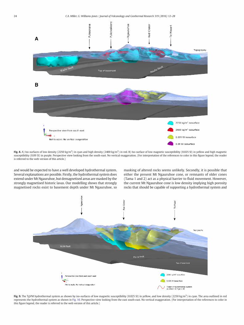
Fig. 8. A) Iso-surfaces of low density (2250 kg/m3) in cyan and high density (2400 kg/m3) in red. B) Iso-surface of low magnetic susceptibility (0.025 SI) in yellow and high magneticsusceptibility (0.09 SI) in purple. Perspective view looking from the south-east. No vertical exaggeration. (For interpretation of the references to color in this figure legend, the readeris referred to the web version of this article.)


and would be expected to have a well developed hydrothermal system.Several explanations are possible. Firstly, the hydrothermal systemdoesextendunderMtNgauruhoe, but demagnetised areas aremaskedby thestrongly magnetised historic lavas. Our modelling shows that stronglymagnetised rocks exist to basement depth under Mt Ngauruhoe, so

Fig. 9. The TgVM hydrothermal system as shown by iso-surfaces of low magnetic susceptibilrepresents the hydrothermal system as shown in Fig. 10. Perspective view looking from the ethis figure legend, the reader is referred to the web version of this article.)

masking of altered rocks seems unlikely. Secondly, it is possible thateither the present Mt Ngauruhoe cone, or remnants of older cones(Tama 1 and 2) act as a physical barrier to fluid movement. However,the current Mt Ngauruhoe cone is low density implying high porosityrocks that should be capable of supporting a hydrothermal system and

ity (0.025 SI) in yellow, and low density (2250 kg/m3) in cyan. The area outlined in redast south-east. No vertical exaggeration. (For interpretation of the references to color in

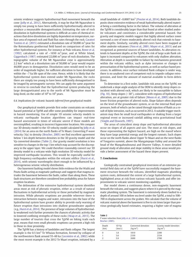
Table 2P wave velocities from Jolly et al. (2014) converted to density using the relationships inBrocher (2005).

Depth(km)

1D Vp(km/s)

Converted densities(kg/m3)

Gravity model densities(kg/m3)

0 1.8 1810 22001 3.6 2330 23342 5.9 2690 2700


seismic evidence suggests hydrothermal fluid movement beneath thecone (Jolly et al., 2012). Alternatively, it may be that Mt Ngauruhoe issimply too young to have been sufficiently hydrothermally altered toproduce a measurable demagnetisation. Estimating the rate of rockdissolution in hydrothermal systems is difficult as rates of chemical re-actions that drivedissolution are highly dependent on temperature, sur-face area of exposed rock and fluid flux rates through the rock. CaratoriTontini et al. (2015) estimated a dissolution rate of 50,000 m3/year forthe Rotomahana geothermal field based on comparison of rates forother hydrothermal systems. For instance at Poás volcano, Rowe et al.(1992) calculated a rate of ~1650 m3/year, and at White Island,Giggenbach (1987) estimated 22,000 m3/year of rock dissolution. Thetopographic volume of the Mt Ngauruhoe cone is approximately2.2 km3 which at a dissolution rate of 50,000 m3/year would require44,000 years to demagnetise. Dissolution rates would need to be anorder of magnitude higher, for sufficient alteration to have developedwithin the ~7 ka life span of the cone. Hence, while it is likely that thehydrothermal system does extend under Mt Ngauruhoe, the rocksthere are simply too young to have been sufficiently demagnetised tobe imaged by aeromagnetic surveys. We can apply the same argumentin reverse to conclude that the hydrothermal system producing thelarge demagnetisated area to the north of Mt Ngauruhoe must belong-lived, on the order of 104 to 105 years.

6.4. Implications for volcanic hazards inferred from geophysical models

Our geophysical models provide first order constraints on volcanichazard potential at TgVM and offer some possibility for improvementsin hazard monitoring. Use of simple 1D seismic velocity models involcanic earthquake location algorithms can impact real-timehazard assessment in times of volcanic unrest if those models areoversimplified, resulting in incorrect hypocenter locations.We compareour 3D density model to the 1D velocity model calculated by Jolly et al.(2014) for an area on the north flanks of Te Maari. Converting P-wavevelocity (Vp) to density (Brocher, 2005) we find excellent agreementbelow 1 km depth between densities in the 3D gravity model and theVp converted densities (Table 2). Our gravity model resolution is lesssensitive to changes in the top 1 kmwhichmay account for the discrep-ancy in the upper layer. We could therefore reasonably convert our 3Ddensity model to a volcano wide high resolution 3D velocity model forimproved earthquake locations. This would be especially useful forhigh frequency earthquakes within the volcanic edifice (Hurst et al.,2014), with seismic wavelengths short enough to be influenced by aheterogeneous seismic velocity distribution.

Our basement faultingmodel shows little evidence for theWaihi andPoutu faults acting asmagmatic pathways and suggests that magma in-trudes the basement between the faults, rather than along them. Thesefault structures are therefore considered low probability areas for futureeruption locations.

The delineation of the extensive hydrothermal system identifiesareas most at risk of phreatic eruption, either as a result of naturalfluctuations in hydrothermal activity or those perturbed by magmaticintrusion. While phreatic eruptions are possible wherever there isinteraction between magma and water, intrusions into the base of thehydrothermal system have greater ability to provide early warning offuture eruption than intrusions into shallow groundwater aquifers(e.g., Hurst et al., 2014). The presence of large volumes of hydrothermal-ly weakened rock further promotes the chances of phreatic activity dueto lowered confining strengths of these rocks (Heap et al., 2015). Thelarge number of tourists that cross the TgVM on hiking trails eachyear, means that even small phreatic eruptions can present a high riskto those in close proximity.

The TgVM has a history of landslides and flank collapse. The largestexample is the 0.5 km3 Te Whaiau formation, formed by collapse ofthe northwestern flank around 55–60 ka (Lecointre et al., 2002) whilethe most recent example is the 2012 Te Maari eruption, initiated by a

small landslide of ~0.0007 km3 (Procter et al., 2014). Both landslide de-posits show extensive evidence of weak hydrothermally alteredmateri-al being a contributing factor in the failure. The volume of alteration atthe TgVM is considerably larger than that found at other studied andes-ite volcanoes and constitutes a considerable potential hazard. Ourgravity and magnetic models suggest that highly altered surface zonessurround a core of more moderately altered rock that extends to base-ment depths. Similarly, variably altered cores have been mapped atother andesite volcanoes (Finn et al., 2001; Mayer et al., 2015) and arerecognised as potential sources of future landslides. As alteration ex-tends to basement depths at the TgVM, the risk of large scale flank col-lapse is increased compared to volcanoes with only shallow alteration.Alteration at depth is susceptible to failure by mechanisms generatedwithin the volcanic edifice, such as dyke intrusion or changes inpressurisation of the hydrothermal system, aswell as surface based pro-cesses. In addition, once surface initiated flank collapse is under way,there is no unaltered core of competent rock to impede collapse retro-gression, and limit the amount of material available to form debrisflows.

To determine to a first order, landslide risk areas on the TgVM, weundertook a slope angle analysis of the DEM to identify steep slopes co-incident with altered rock, which are likely to be susceptible to failure(Fig. 10). Steep slopes (N30°), coincident with regions of hydrothermalalteration, are at greater risk of failure (Moon et al., 2005) due to thelower friction properties of altered rocks. Slope failure often dependson the level of the groundwater system, or on the internal fluid porepressure, both of which can be raised through injection of fluids as a re-sult of dyke intrusion, such as occurred in 2012. A suitable triggermech-anism may then be small local earthquakes or shaking from a largerregional event or increased rainfall adding extra gravitational load(Voight and Elsworth, 1997).

The areas of coincident steep slope and hydrothermal alterationoccur on slopes of all aspects and size. The most at risk slopes, andthose representing the highest hazard, are high on the massif wherethey have large potential energy and the longest runouts. Such slopesoccur on the north flanks above Upper Te Maari and on the west flanksof Tongariro summit, above the Mangatepopo Valley and around thehead of the Mangahouhounui and Oturere Valleys. A more detailedground study of alteration and slope stability in these areas would pro-vide a better assessment of the hazard these slopes present.

7. Conclusions

Geologically constrained geophysical inversions of an extensive po-tential field data set at the TgVM have successfully mapped the base-ment structure beneath the volcano, identified magmatic plumbingsystem roots, delineated the extent of a large hydrothermal system,highlighted areas at risk from various volcanic hazards and offer im-provements to volcanic unrest monitoring capability.

Our model shows a continuous dense, non-magnetic basementbeneath the volcano, and suggests placeswhere it is pierced by themag-matic plumbing system. The basement is extensively down faulted to adepth of around 100m below sea level under the TgVM, a total to 500–700m displacement across the graben.We calculate that the volume ofvolcanicmaterial above the basement is five to six times larger thanpre-vious geologically based estimates, requiring a higher rate of magma

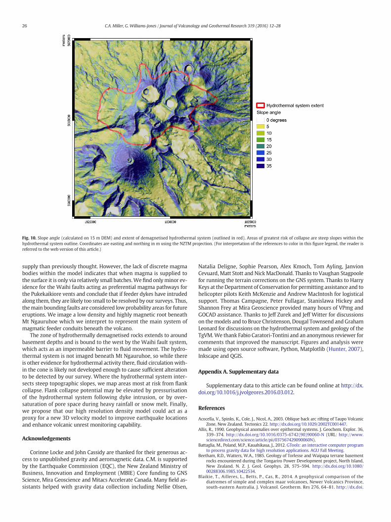
Fig. 10. Slope angle (calculated on 15 m DEM) and extent of demagnetised hydrothermal system (outlined in red). Areas of greatest risk of collapse are steep slopes within thehydrothermal system outline. Coordinates are easting and northing in m using the NZTM projection. (For interpretation of the references to color in this figure legend, the reader isreferred to the web version of this article.)


supply than previously thought. However, the lack of discrete magmabodies within the model indicates that when magma is supplied tothe surface it is only via relatively small batches.We find onlyminor ev-idence for the Waihi faults acting as preferential magma pathways forthe Pukekaikiore vents and conclude that if feeder dykes have intrudedalong them, they are likely too small to be resolved by our surveys. Thus,themain bounding faults are considered low probability areas for futureeruptions. We image a low density and highly magnetic root beneathMt Ngauruhoe which we interpret to represent the main system ofmagmatic feeder conduits beneath the volcano.

The zone of hydrothermally demagnetised rocks extends to aroundbasement depths and is bound to the west by the Waihi fault system,which acts as an impermeable barrier to fluid movement. The hydro-thermal system is not imaged beneath Mt Ngauruhoe, so while thereis other evidence for hydrothermal activity there, fluid circulation with-in the cone is likely not developed enough to cause sufficient alterationto be detected by our survey. Where the hydrothermal system inter-sects steep topographic slopes, we map areas most at risk from flankcollapse. Flank collapse potential may be elevated by pressurisationof the hydrothermal system following dyke intrusion, or by over-saturation of pore space during heavy rainfall or snow melt. Finally,we propose that our high resolution density model could act as aproxy for a new 3D velocity model to improve earthquake locationsand enhance volcanic unrest monitoring capability.

Acknowledgements

Corinne Locke and John Cassidy are thanked for their generous ac-cess to unpublished gravity and aeromagnetic data. C.M. is supportedby the Earthquake Commission (EQC), the New Zealand Ministry ofBusiness, Innovation and Employment (MBIE) Core funding to GNSScience, Mira Geoscience and Mitacs Accelerate Canada. Many field as-sistants helped with gravity data collection including Nellie Olsen,

Natalia Deligne, Sophie Pearson, Alex Kmoch, Tom Ayling, JanvionCevuard, Matt Stott and NickMacDonald. Thanks to Vaughan Stagpoolefor running the terrain corrections on the GNS system. Thanks to HarryKeys at theDepartment of Conservation for permitting assistance and tohelicopter pilots Keith McKenzie and Andrew MacIntosh for logisticalsupport. Thomas Campagne, Peter Fullagar, Stanislawa Hickey andShannon Frey at Mira Geoscience provided many hours of VPmg andGOCAD assistance. Thanks to Jeff Zurek and Jeff Witter for discussionson themodels and to Bruce Christenson, Dougal Townsend andGrahamLeonard for discussions on the hydrothermal system and geology of theTgVM.We thank Fabio Caratori-Tontini and an anonymous reviewer forcomments that improved the manuscript. Figures and analysis weremade using open source software, Python, Matplotlib (Hunter, 2007),Inkscape and QGIS.

Appendix A. Supplementary data

Supplementary data to this article can be found online at http://dx.doi.org/10.1016/j.jvolgeores.2016.03.012.

References

Acocella, V., Spinks, K., Cole, J., Nicol, A., 2003. Oblique back arc rifting of Taupo VolcanicZone, New Zealand. Tectonics 22. http://dx.doi.org/10.1029/2002TC001447.

Allis, R., 1990. Geophysical anomalies over epithermal systems. J. Geochem. Explor. 36,339–374. http://dx.doi.org/10.1016/0375-6742(90)90060-N (URL: http://www.sciencedirect.com/science/article/pii/037567429090060N).

Battaglia, M., Poland, M.P., Kauahikaua, J., 2012. GTools: an interactive computer programto process gravity data for high resolution applications. AGU Fall Meeting.

Beetham, R.D., Watters, W.A., 1985. Geology of Torlesse and Waipapa terrane basementrocks encountered during the Tongariro Power Development project, North Island,New Zealand. N. Z. J. Geol. Geophys. 28, 575–594. http://dx.doi.org/10.1080/00288306.1985.10422534.

Blaikie, T., Ailleres, L., Betts, P., Cas, R., 2014. A geophysical comparison of thediatremes of simple and complex maar volcanoes, Newer Volcanics Province,south-eastern Australia. J. Volcanol. Geotherm. Res 276, 64–81. http://dx.doi.


org/10.1016/j.jvolgeores.2014.03.001 (URL: http://linkinghub.elsevier.com/retrieve/pii/S0377027314000717).

Breard, E., Lube, G., Cronin, S., Fitzgerald, R., Kennedy, B., Scheu, B., Montanaro, C., White,J., Tost, M., Procter, J., Moebis, A., 2014. Using the spatial distribution and lithology ofballistic blocks to interpret eruption sequence and dynamics: August 6, 2012 UpperTe Maari eruption, New Zealand. J. Volcanol. Geotherm. Res. 286, 373–386. http://dx.doi.org/10.1016/j.jvolgeores.2014.03.006 (URL: http://linkinghub.elsevier.com/retrieve/pii/S0377027314000936).

Brocher, T.M., 2005. Empirical relations between elastic wavespeeds and density in theEarth's crust. Bull. Seismol. Soc. Am. 95, 2081–2092. http://dx.doi.org/10.1785/0120050077.

Cannavò, F., Camacho, A.G., González, P.J., Mattia, M., Puglisi, G., Fernández, J., 2015. Realtime tracking of magmatic intrusions by means of ground deformation modelingduring volcanic crises. Sci. Rep. 5, 10970. http://dx.doi.org/10.1038/srep10970.

Caratori Tontini, F., Cocchi, L., Muccini, F., Carmisciano, C., Marani, M., Bonatti, E., Ligi, M.,Boschi, E., 2010. Potential-field modeling of collapse-prone submarine volcanoes inthe southern Tyrrhenian Sea (Italy). Geophys. Res. Lett. 37. http://dx.doi.org/10.1029/2009GL041757 (n/a–n/a).

Caratori Tontini, F., de Ronde, C., Scott, B., Soengkono, S., Stagpoole, V., Timm, C., Tivey, M.,2015. Interpretation of gravity and magnetic anomalies at Lake Rotomahana: geolog-ical and hydrothermal implications. J. Volcanol. Geotherm. Res. http://dx.doi.org/10.1016/j.jvolgeores.2015.07.002 (URL: http://linkinghub.elsevier.com/retrieve/pii/S0377027315002103).

Cassidy, J., Locke, C.a., 1995. Geophysical signatures of andesite volcanoes in New Zealand—contrasts and structural implications.

Cassidy, J., Ingham,M., Locke, C.A., Bibby, H., 2009. Subsurface structure across the axis of theTongariro Volcanic Centre, New Zealand. J. Volcanol. Geotherm. Res. 179, 233–240.http://dx.doi.org/10.1016/j.jvolgeores.2008.11.017 (URL: http://linkinghub.elsevier.com/retrieve/pii/S0377027308006100).

Christenson, B.W.,Werner, C.A., Reyes, A.G., Sherburn, S., Scott, B.J., Miller, C., Rosenburg, M.J.,Hurst, A.W., Britten, K.A., 2007. Hazards from hydrothermally sealed volcanic conduits.Eos, Trans. Am. Geophys. Union 88, 53. http://dx.doi.org/10.1029/2007EO050002.

Day, S.J., 1996. Hydrothermal pore fluid pressure and the stability of porous, permeablevolcanoes. Geol. Soc. Lond. Spec. Publ. 110, 77–93. http://dx.doi.org/10.1144/GSL.SP.1996.110.01.06 (URL: http://sp.lyellcollection.org/content/110/1/77).

Finn, C., Sisson, T., Deszcz-Pan, M., 2001. Aerogeophysical measurements of collapse-pronehydrothermally altered zones at Mount Rainier volcano. Nature 409, 600–603. http://dx.doi.org/10.1038/35054533 (URL: http://www.ncbi.nlm.nih.gov/pubmed/11214315).

Finn, C.A., Deszcz-Pan, M., Anderson, E.D., John, D.A., 2007. Three-dimensional geophysi-cal mapping of rock alteration and water content at Mount Adams, Washington:implications for lahar hazards. J. Geophys. Res. 112, B10204. http://dx.doi.org/10.1029/2006JB004783.

Fullagar, P., Pears, G., 2007. Towards geologically realistic inversion. Proceedings of Explo-ration 07: Fifth Decennial International Conference on Mineral Exploration,pp. 444–460 (URL: http://www.dmec.ca/ex07-dvd/E07/pdfs/28.pdf).

Fullagar, P.K., Pears, G.A., McMonnies, B., 2008. Constrained inversion of geologicsurfaces pushing the boundaries. Lead. Edge 27, 98–105. http://dx.doi.org/10.1190/1.2831686.

Giggenbach, W.F., 1987. Redox processes governing the chemistry of fumarolic gas dis-charges from White Island, New Zealand. Appl. Geochem. 2, 143–161. http://dx.doi.org/10.1016/0883-2927(87)90030-8.

Gottsmann, J., Camacho, A.G., Mart, J., Wooller, L., Fernández, J., Garca, A., Rymer, H., 2008.Shallow structure beneath the Central Volcanic Complex of Tenerife fromnew gravitydata: implications for its evolution and recent reactivation. Phys. Earth Planet. Inter.168, 212–230. http://dx.doi.org/10.1016/j.pepi.2008.06.020 (URL: http://linkinghub.elsevier.com/retrieve/pii/S003192010800160X).

Griffin, A.M., 2007. Products and Processes of Cone-building Eruptions from North Crater,Tongariro (Ph.D. thesis) University of Waikato.

Hackett, W.R., 1985. Geology and Petrology of Ruapehu and Related Vents (Ph.D. thesis)Victoria University of Wellington.

Hagerty,M., Benites, R., 2003. Tornillos beneath Tongariro Volcano, New Zealand. J. Volcanol.Geotherm. Res. 125, 151–169. http://dx.doi.org/10.1016/S0377-0273(03)00094-5(URL: http://linkinghub.elsevier.com/retrieve/pii/S0377027303000945).

Heap, M.J., Kennedy, B.M., Pernin, N., Jacquemard, L., Baud, P., Farquharson, J.I., Scheu, B.,Lavallée, Y., Gilg, H.A., Letham-Brake, M., Mayer, K., Jolly, A.D., Reuschlé, T., Dingwell,D.B., 2015. Mechanical behaviour and failure modes in the Whakaari (White Islandvolcano) hydrothermal system, New Zealand. J. Volcanol. Geotherm. Res. 295,26–42. http://dx.doi.org/10.1016/j.jvolgeores.2015.02.012 (URL: http://linkinghub.elsevier.com/retrieve/pii/S037702731500058X).

Hill, G.J., Bibby, H.M., Ogawa, Y., Wallin, E.L., Bennie, S.L., Caldwell, T.G., Keys, H.,Bertrand, E.A., Heise, W., 2015. Structure of the Tongariro Volcanic system:insights from magnetotelluric imaging. Earth Planet. Sci. Lett. 432, 115–125.http://dx.doi.org/10.1016/j.epsl.2015.10.003 (URL: http://linkinghub.elsevier.com/retrieve/pii/S0012821X15006305).

Hinze, W.J., Aiken, C., Brozena, J., Coakley, B., Dater, D., Flanagan, G., Forsberg, R.,Hildenbrand, T., Keller, G.R., Kellogg, J., Kucks, R., Li, X., Mainville, A., Morin, R.,Pilkington, M., Plouff, D., Ravat, D., Roman, D., Urrutia-Fucugauchi, J., Veronneau, M.,Webring, M., Winester, D., 2005. New standards for reducing gravity data: theNorth American gravity database. Geophysics 70, J25–J32. http://dx.doi.org/10.1190/1.1988183 (URL: http://scholarcommons.sc.edu/geol_facpub/2).

Hobden, B.J., 1997. Modelling Magmatic Trends in Time and Space: Eruptive and MagmaticHistory of the Tongariro Volcanic Complex, New Zealand (Ph.D. thesis) University ofWaikato.

Hobden, B.J., Houghton, B.F., Lanphere, M.A., Nairn, I.A., 1996. Growth of the Tongarirovolcanic complex: new evidence from KAr age determinations. N. Z. J. Geol. Geophys.39, 151–154. http://dx.doi.org/10.1080/00288306.1996.9514701.

Hobden, B.J., Houghton, B.F., Davidson, J.P., Weaver, S.D., 1999. Small and short-livedmagma batches at composite volcanoes: time windows at Tongariro volcano, NewZealand. J. Geol. Soc. 156, 865–868. http://dx.doi.org/10.1144/gsjgs.156.5.0865.

Hochstein, M., 1985. Steaming Ground at Red Crater and in the Te Maari Craters.Hunt, T., Mumme, T., 1986. Some magnetic properties of two recent lava flows from

Mount Ngauruhoe, Tongariro Volcanic Centre, New Zealand. J. R. Soc. N. Z. 16,71–83. http://dx.doi.org/10.1080/03036758.1986.10426957.

Hunter, J., 2007. Matplotlib: a 2D graphics environment. Comput. Sci. Eng. 9, 90–95.Hurst, T., Jolly, A.D., Sherburn, S., 2014. Precursory characteristics of the seismicity before the

6 August 2012 eruption of Tongariro volcano, North Island, New Zealand. J. Volcanol.Geotherm. Res. 286, 294–302. http://dx.doi.org/10.1016/j.jvolgeores.2014.03.004(URL: http://linkinghub.elsevier.com/retrieve/pii/S0377027314000821).

Johnson, J.H., Savage, M.K., 2012. Tracking volcanic and geothermal activity in the TongariroVolcanic Centre, New Zealand, with shear wave splitting tomography. J. Volcanol.Geotherm. Res. 223-224, 1–10. http://dx.doi.org/10.1016/j.jvolgeores.2012.01.017(URL: http://linkinghub.elsevier.com/retrieve/pii/S0377027312000303).

Johnson, J.H., Savage, M.K., Townend, J., 2011. Distinguishing between stress-induced andstructural anisotropy at Mount Ruapehu volcano, New Zealand. J. Geophys. Res. 116,B12303. http://dx.doi.org/10.1029/2011JB008308.

Jolly, A.D., Chardot, L., Neuberg, J., Fournier, N., Scott, B.J., Sherburn, S., 2012. High impactmass drops from helicopter: a new active seismic source method applied in an activevolcanic setting. Geophys. Res. Lett. 39. http://dx.doi.org/10.1029/2012GL051880(n/a–n/a).

Jolly, A., Lokmer, I., Kennedy, B., Keys, H., Proctor, J., Lyons, J., Jolly, G., 2014. Active seismicsources as a proxy for seismic surface processes: an example from the 2012 Tongarirovolcanic eruptions, New Zealand. J. Volcanol. Geotherm. Res. 286, 317–330. http://dx.doi.org/10.1016/j.jvolgeores.2014.04.008 (URL: http://linkinghub.elsevier.com/retrieve/pii/S0377027314001188).

Jones, E., Oliphant, T.E., Peterson, P., 2001. Scipy: Open Source Scientific Tools for Python.Krippner, J.B., 2009. Ngauruhoe Inner Crater Volcanic Processes of the 1954–55 and

1974–75 Eruptions (Ph.D. thesis) University of Waikato.Lecointre, J.A., Neall, V.E., Wallace, C.R., Prebble, W.M., 2002. The 55- to 60-ka Te Whaiau

Formation: a catastrophic, avalanche-induced, cohesive debris-flow deposit fromProto-Tongariro Volcano, New Zealand. Bull. Volcanol. 63, 509–525. http://dx.doi.org/10.1007/s004450100167.

Lee, J., Townsend, D., Bland, K., Kamp, P., 2011. Geology of the Hawkes Bay Area. TechnicalReport. GNS Science.

Locke, C.A., Cassidy, J., MacDonald, A., 1993. Three-dimensional structure of relict strato-volcanoes in Taranaki, New Zealand: evidence from gravity data. J. Volcanol.Geotherm. Res. 59, 121–130. http://dx.doi.org/10.1016/0377-0273(93)90081-2(URL: http://linkinghub.elsevier.com/retrieve/pii/0377027393900812).

López, D.L., Williams, S.N., 1993. Catastrophic volcanic collapse: relation to hydrothermalprocesses. Science (New York, N.Y.) 260, 1794–1796. http://dx.doi.org/10.1126/science.260.5115.1794.

Mayer, K., Scheu, B., Gilg, H.A., Heap, M.J., Kennedy, B.M., Lavallée, Y., Letham-Brake, M.,Dingwell, D.B., 2015. Experimental constraints on phreatic eruption processes atWhakaari (White Island volcano). J. Volcanol. Geotherm. Res. 302, 150–162. http://dx.doi.org/10.1016/j.jvolgeores.2015.06.014 (URL: http://linkinghub.elsevier.com/retrieve/pii/S0377027315001900).

McNamara, D., Faulkner, D., McCarney, E., 2014. Rock properties of greywacke basementhosting geothermal reservoirs, New Zealand: preliminary results. Thirty-NinthWork-shop on Geothermal Reservoir Engineering, pp. 1–10.

Milicich, S., Wilson, C., Bignall, G., Pezaro, B., Bardsley, C., 2013. Reconstructing the geologicaland structural history of an active geothermal field: a case study from New Zealand.J. Volcanol. Geotherm. Res. 262, 7–24. http://dx.doi.org/10.1016/j.jvolgeores.2013.06.004 (URL: http://linkinghub.elsevier.com/retrieve/pii/S0377027313001789).

Moebis, A., Cronin, S.J., Neall, V.E., Smith, I.E., 2011. Unravelling a complex volcanic historyfrom fine-grained, intricate Holocene ash sequences at the Tongariro Volcanic Centre,New Zealand. Quat. Int. 246, 352–363. http://dx.doi.org/10.1016/j.quaint.2011.05.035(URL: http://linkinghub.elsevier.com/retrieve/pii/S1040618211003089).

Moon, V., Bradshaw, J., Smith, R., de Lange, W., 2005. Geotechnical characterisation ofstratocone crater wall sequences, White Island Volcano, New Zealand. Eng. Geol.81, 146–178. http://dx.doi.org/10.1016/j.enggeo.2005.07.014.

Morelli, C., Gantar, C., Honkasalo, T., McConnel, R., Tanner, J., Szabo, B., Uotila, U., Whalen, C.,1974. The International Gravity Standardisation Net 1971 (IGSN71). Special PublicationNo. 4.

Nairn, I.A., 2000. The; 10 ka multiple vent pyroclastic eruption sequence at TongariroVolcanic Centre, Taupo Volcanic Zone, New Zealand: part 1. Eruptive processesduring regional extension. J. Volcanol. Geotherm. Res. 19–44.

Nettleton, L.L., 1939. Determination of density for reduction of gravimeter observations.Geophysics 4. http://dx.doi.org/10.1190/1.1437088.

Parasnis, D., 1966. Mining Geophysics. Elsevier, Amsterdam–London–New York.Pardo, N., Cronin, S., Palmer, A., Procter, J., Smith, I., 2012. Andesitic Plinian eruptions at

Mt. Ruapehu: quantifying the uppermost limits of eruptive parameters. Bull.Volcanol. 74, 1161–1185. http://dx.doi.org/10.1007/s00445-012-0588-y.

Pardo, N., Cronin, S.J., Németh, K., Brenna, M., Schipper, C.I., Breard, E., White, J.D., Procter,J., Stewart, B., Agustn-Flores, J., Moebis, A., Zernack, A., Kereszturi, G., Lube, G., Auer,A., Neall, V., Wallace, C., 2014. Perils in distinguishing phreatic from phreatomagmaticash; insights into the eruption mechanisms of the 6 August 2012Mt. Tongariro erup-tion, New Zealand. J. Volcanol. Geotherm. Res. 286, 397–414. http://dx.doi.org/10.1016/j.jvolgeores.2014.05.001 (URL: http://linkinghub.elsevier.com/retrieve/pii/S037702731400136X).

Potter, S.H., Jolly, G.E., Neall, V.E., Johnston, D.M., Scott, B.J., 2014. Communicating the sta-tus of volcanic activity: revising New Zealands volcanic alert level system. J. Appl.Volcanol. 3, 13. http://dx.doi.org/10.1186/s13617-014-0013-7 (URL: http://www.appliedvolc.com/content/3/1/13).


Procter, J., Cronin, S., Zernack, A.V., Lube, G., Stewart, R., Nemeth, K., Keys, H., 2014. Debrisflow evolution and the activation of an explosive hydrothermal system; Te Maari,Tongariro, New Zealand. J. Volcanol. Geotherm. Res. 286, 303–316. http://dx.doi.org/10.1016/j.jvolgeores.2014.07.006 (URL: http://linkinghub.elsevier.com/retrieve/pii/S0377027314002170).

Reid, M.E., Sisson, T.W., Brien, D.L., 2002. Volcano collapse promoted by hydrothermalalteration and edifice shape, Mount Rainier, Washington. Geology 29, 779–782.http://dx.doi.org/10.1130/0091-7613(2001)029b0779:VCPBHAN2.0.CO;2.

Rowe, G.L., Brantley, S.L., Fernandez, M., Fernandez, J.F., Borgia, A., Barquero, J., 1992.Fluid–volcano interaction in an active stratovolcano: the crater lake system of Poásvolcano, Costa Rica. J. Volcanol. Geotherm. Res. 49, 23–51. http://dx.doi.org/10.1016/0377-0273(92)90003-V.

Rowland, J.V., Sibson, R.H., 2001. Extensional fault kinematics within the Taupo VolcanicZone, New Zealand: softlinked segmentation of a continental rift system. N. Z.J. Geol. Geophys. 44, 271–283. http://dx.doi.org/10.1080/00288306.2001.9514938.

Rowlands, D.P., White, R.S., Haines, A.J., 2005. Seismic tomography of the Tongariro Volca-nic Centre, New Zealand. Geophys. J. Int. 163, 1180–1194. http://dx.doi.org/10.1111/j.1365-246X.2005.02716.x.

Sanders, F., 2010. Rheology and Flow Emplacement Processes of the 1954 Lavas, MountNgauruhoe Ph.D. thesis University of Waikato.

Sano, Y., Kagoshima, T., Takahata, N., Nishio, Y., Roulleau, E., Pinti, D.L., Fischer, T.P., 2015.Ten-year helium anomaly prior to the 2014 Mt. Ontake eruption. Sci. Rep. 5, 13069.http://dx.doi.org/10.1038/srep13069.

Scott, B.J., Potter, S.H., 2014. Aspects of historical eruptive activity and volcanic unrest atMt. Tongariro, New Zealand: 18462013. J. Volcanol. Geotherm. Res. 286, 263–276.http://dx.doi.org/10.1016/j.jvolgeores.2014.04.003 (URL: http://linkinghub.elsevier.com/retrieve/pii/S0377027314001127).

Seebeck, H., Nicol, A., Villamor, P., Ristau, J., Pettinga, J., 2014. Structure and kinematics ofthe Taupo Rift, New Zealand. Tectonics 33, 1178–1199. http://dx.doi.org/10.1002/2014TC003569.

Simons, B.C., 2014. Volcanic History and Eruption Processes of Blue Lake Crater, TongariroPh.D. thesis University of Waikato.

Spector, A., 1970. Statistical Models for Interpreting Aeromagnetic Data. http://dx.doi.org/10.1190/1.1440092.

Stagpoole, V.M., Bibby, H.M., 1999. Residual gravity anomaly of the Taupo Volcanic Zone,New Zealand, 1:250,000. Technical Report. Institute of Geological and NuclearSciences.

Stern, T.A., 1979. Regional and residual gravity fields, central North Island, New Zealand.N. Z. J. Geol. Geophys. 22, 479–485. http://dx.doi.org/10.1080/00288306.1979.10424156.

Thébault, E., Finlay, C.C., Beggan, C.D., Alken, P., Aubert, J., Barrois, O., Bertrand, F., Bondar,T., Boness, A., Brocco, L., Canet, E., Chambodut, A., Chulliat, A., Cosson, P., Civet, F., Du,A., Fournier, A., Fratter, I., Gillet, N., Hamilton, B., Hamoudi, M., Hulot, G., Jager, T.,Korte, M., Kuang, W., Lalanne, X., Langlais, B., Léger, J.M., Lesur, V., Lowes, F.J.,Macmillan, S., Mandea, M., Manoj, C., Maus, S., Olsen, N., Petrov, V., Ridley, V.,Rother, M., Sabaka, T.J., Saturnino, D., Schachtschneider, R., Sirol, O., Tangborn, A.,Thomson, A., Tøffner-Clausen, L., Vigneron, P., Wardinski, I., Zvereva, T., 2015. Interna-tional geomagnetic reference field: the 12th generation. Earth, Planets Space 67, 79.http://dx.doi.org/10.1186/s40623-015-0228-9 (URL: http://www.earth-planets-space.com/content/67/1/79).

Tontini, F.C., de Ronde, C.E.J., Kinsey, J.C., Soule, A., Yoerger, D., Cocchi, L., 2013. Geophys-ical modeling of collapse-prone zones at Rumble III seamount, southern PacificOcean, New Zealand. Geochem. Geophys. Geosyst. 14, 4667–4680. http://dx.doi.org/10.1002/ggge.20278.

van Wyk de Vries, B., Borgia, A., 1996. The role of basement in volcano deformation. Geol.Soc. Lond. Spec. Publ. 110, 95–110. http://dx.doi.org/10.1144/GSL.SP.1996.110.01.07.

Villamor, P., Berryman, K.R., 2006a. Evolution of the southern termination of the TaupoRift, New Zealand. N. Z. J. Geol. Geophys. 49, 23–37. http://dx.doi.org/10.1080/00288306.2006.9515145.

Villamor, P., Berryman, K.R., 2006b. Late Quaternary geometry and kinematics of faults atthe southern termination of the Taupo Volcanic Zone, New Zealand. N. Z. J. Geol.Geophys. 49, 1–21. http://dx.doi.org/10.1080/00288306.2006.9515144.

Voight, B., Elsworth, D., 1997. Failure of volcano slopes. http://dx.doi.org/10.1680/geot.1997.47.1.1.

Wadsworth, F.B., Kennedy, B.M., Branney, M.J., von Aulock, F.W., Lavallée, Y., Menendez,A., 2015. Exhumed conduit records magma ascent and drain-back during aStrombolian eruption at Tongariro volcano, New Zealand. Bull. Volcanol. 77, 71.http://dx.doi.org/10.1007/s00445-015-0962-7.

Walsh, F., Hochstein, M., Bromley, C., 1998. The Tongariro Geothermal System. Review ofGeophysical Data.

Wessel, P., Smith, W., 2013. Generic mapping tools: inproved version released. EOS Trans.AGU 94, 409–410.

White, S., Crisp, J.A., Spera, F., 2006. Longterm volumetric eruption rates and magmabudgets. Geochem. Geophys. 7, Q03010. http://dx.doi.org/10.1029/2005GC001002.

Zeng, Y., Ingham, M., 1993. Modelling of gravity data from Tongariro National Park. 15thNZ Geothermal Workshop, pp. 219–226.

Supplementary material for “Internal structure andvolcanic hazard potential of Mt Tongariro, New

Zealand, from 3D geologically constrained gravity andmagnetic models”

C. A. Millera,b,∗, G. Williams-Jonesa

aDepartment of Earth Sciences, Simon Fraser University , Burnaby, BC V5A 1S6, CanadabGNS Science, Wairakei Research Centre, Private Bag 2000, Taupo, 3352, New Zealand

1. Geophysical model

The geophysical model is supplied as a Geoscience Analyst project file for

visualisation. The model file can be downloaded from http://tinyurl.com/

ntw5tel.

Geoscience Analyst may be obtained free of charge from Mira Geoscience,

http://www.mirageoscience.com/our-products/software-product/geoscience-analyst.

2. Gravity data correction scheme.

We corrected data to the ellipsoid height datum as our heights are largely de-

rived from GNSS (WGS84 datum) measurements. Orthometric heights from the

older surveys were converted to ellipsoid heights using a geoid model (NZVGD09)

from Land Information New Zealand, so that they could be processed in a uni-

form manner with the new stations. We corrected all data for latitude variations

using the theoretical gravity value from 1980 GRS Geodetic Reference System

(GRS80) formula. As our survey covers a large range of elevations (600 to 2300

m.a.s.l.) we applied an atmospheric correction to account for the changing den-

sity of atmosphere. We applied the free air correction using the full equation

∗Corresponding authorEmail address: [email protected] (C. A. Miller)

Preprint submitted to Journal of Volcanology and Geothermal Research November 14, 2015

with second order terms and applied a Bouguer correction, with the curvature

correction included. Finally we applied terrain corrections in a 3 step process.

Firstly, inner terrain corrections out to Hammer Zone D were estimated in the

field and then calculated using Hammer’s formula (Hammer, 1939). We then

applied outer corrections using an 8 m DEM for Zones E and F and used a 15

m DEM for corrections in zones G to M. The terrain corrections represent one

of the larger sources of error. Comparison of the manual inner (B-D) correc-

tions with those from the 8 m DEM show a mean variation of 0.04 mGal. To

estimate errors in the outer zones (E-M) we computed terrain corrections with

an 8 m DEM and a 15 m DEM and calculate an RMS error in the differences

between the two of 0.045 mGal. The DEMs used for terrain corrections do not

take into account the bathymetry of lakes and as such the terrain corrections

may be over-estimated due to low density water being corrected as denser rock

(Hasegawa et al., 2009). Lake Taupo is New Zealand’s largest lake (616 km2)

and is located 13 km north of the model area, but is within the broader area

used to determine the regional field. To determine the gravity effect of the lake,

we constructed a forward model using a slab with the approximate outline of the

lake and a thickness of 100 m (the average lake depth). The maximum gravity

effect at a station directly on the lake shore is 6 mGal, reducing to 0.02 mGal

for the nearest station within our modelling area. We subtracted the gravity

signal of Lake Taupo from our terrain correction value to ensure our stations

used for regional field determination are properly corrected. The smaller Lake

Rotoaira (13 km2), directly on the north edge of the model area, is on average 10

m deep and has a maximum gravity effect at the closest station of 0.023 mGal.

This is within our noise envelope so we did not apply a further correction. No

corrections were applied for the many small lakes on Mt Tongariro as they are

too small to produce a measurable gravity effect.

2

3. Bulk Density from Gravity Measurements

The Nettleton (Nettleton, 1939) and Parasnis (Parasnis, 1966) methods pro-

vide means of estimating bulk density from minimisation of the correlation of

Bouguer and terrain corrected gravity with topography and variants of these

methods have been applied in several volcano studies (Gottsmann et al., 2008;

Hautmann et al., 2013). We compare calculated bulk density estimations to

rock physical property measurements to determine the optimal gravity correc-

tion density. An important and often overlooked caveat for both methods is that

there is no direct causation of the topography by the geology, i.e., that dense

rocks do not form high peaks or vice versa. This assumption can be difficult

to verify in volcanic terranes where high standing ridges are often composed of

denser, more erosion resistant material such as lava flows, while lower density

pyroclastics fill valley floors. Both methods also rely on there being no regional

affect in the gravity data which could bias the analysis. To minimise these re-

strictions, we selected data from 156 stations located between the Waihi and

Poutu fault zones where Cassidy et al. (2009) showed that the regional field is

relatively flat. These data should be mostly free of long wavelength variations

caused by large scale faulting and regional gravity changes, and best represent

the bulk density of the volcano superstructure from 1300 to 2300 m elevation.

For Nettleton’s method we calculated the Pearson correlation coefficient be-

tween the Bouguer gravity and elevation for a range of Bouguer and terrain

correction densities. The correlation coefficient closest to zero, corresponds to

the bulk terrain density of 2025 kg/m3 (Supplementary figure 1). We used the

same data set for Paranis method and ran an ordinary least squares regression

on the free air anomaly against the elevation data. The density is retrieved by

the relation: density = regression slope / 2πG, where G is the universal gravity

constant (Supplementary figure 2). All except two points plot within the 95%

confidence interval of the best fit regression line. These points are located on

the summit of Ngauruhoe and hand specimen densities from the 1954 summit

cone are the lowest in the physical property dataset, between 498 - 731 kg/m3.

3

As these points are outside the 95% confidence bounds, they are excluded from

the regression analysis. The retrieved density is 2029 ± 36 kg/m3and agrees

very well with the density retrieved from Nettleton’s method. The bulk density

values retrieved by Nettleton’s and Parasnis’s methods are close to the mean

wet density of pyroclastic materials sampled (1931 ± 267 kg/m3). However, this

density appears to be too low as andesite lava (wet density 2535 ± 205kg/m3),

makes up a sizeable proportion of the massif (Supplementary Figure 3. We in-

terpret this discrepancy as due to a violation of the assumptions of Nettleton’s

and Paranis’s method, implying that even with careful data selection there is

still an implicit correlation between the topography and density. As such we use

our physical property measurements for the correction density (Supplementary

figure 3).

4. Inversion method

VPmg solves the inversion using the steepest descent method, where no ma-

trix inversion is required (Fullagar and Pears, 2007). For the conventional least

squares inversion, the objective at each iteration is the smallest parameter per-

turbation required to halve the L2 -norm data misfit. Stochastic inversion is an

option for heterogeneous property inversion of either basement or other units.

In this case, individual model cells are subjected to random property perturba-

tions; the perturbation is accepted if it produces a reduction in misfit and if it is

compatible with the expected property distribution within the geological unit.

Maximum perturbation size is defined in terms of absolute property change,

for property inversion, or in terms of fractional change in depth, for geometry

inversion. Degree of fit is determined by the magnitude of the chi-squared data

norm, L2, and the L1- data norm, defined by

L2 = 1/NN∑

n=1

[on − cnεn

]2(1)

L1 = 1/N√π/2

N∑n=1

∣∣∣∣on − cnεn

∣∣∣∣ (2)

4

where N is the number of data, On is the measured data, Cn the calculated

model response and εn the uncertainty (standard deviation) applied to the nth

data point. If the data uncertainties are controlled by normal random variables

with zero mean, the both L2 and L1 have expected values of unity. Therefore,

the model is deemed acceptable if L2 <1 and/or if L1 <1. For a starting εn, we

used a value of 10% of the standard deviation of the range of observed data. If

a model converges with this εn we successively lower the εn until the inversion

stalls, at which point we have achieved the best fit possible.

The L1 and L2 misfits are dimensionless, as they are normalised by the

uncertainties, εn.

A depth weighting is applied to lower the sensitivity of the inversion to

deeper cells, with the aim of creating ”smaller” bodies and limiting the smearing

of bodies with depth.

5. Gravity results

5.1. Apparent Density Inversion

We begin our exploration of the gravity data by performing an ‘apparent

density’ (AD) inversion. An AD model is a voxet with only 1 cell per vertical

prism (i.e. the cell vertical extent is the same as the whole voxet) and the

inversion adjusts the density in each prism until the calculated response of the

model matches the input data. Apparent density models are useful for looking

at lateral density variations in the dataset. The result of the apparent density

inversion is seen in Supplementary Figure 4A. We use a diverging colour scheme

to highlight areas of higher and lower density, relative to the Bouguer correction

density of 2300 kg/m3. The model has an RMS misfit of 1.0 mGal which is

relatively high and indicates that a more detailed model which incorporates

vertical density variations is required .

The residual gravity (observed - calculated) map (Supplementary Figure 4B)

shows the highest areas of misfit are under the main part of the volcanic edifice,

where the geology is likely to be highly three dimensional. Areas of high positive

5

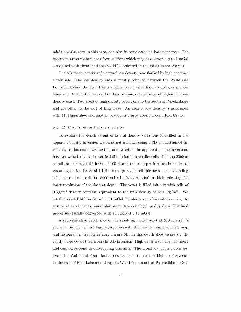
misfit are also seen in this area, and also in some areas on basement rock. The

basement areas contain data from stations which may have errors up to 1 mGal

associated with them, and this could be reflected in the misfit in these areas.

The AD model consists of a central low density zone flanked by high densities

either side. The low density area is mostly confined between the Waihi and

Poutu faults and the high density region correlates with outcropping or shallow

basement. Within the central low density zone, several areas of higher or lower

density exist. Two areas of high density occur, one to the south of Pukekaikiore

and the other to the east of Blue Lake. An area of low density is associated

with Mt Ngauruhoe and another low density area occurs around Red Crater.

5.2. 3D Unconstrained Density Inversion

To explore the depth extent of lateral density variations identified in the

apparent density inversion we construct a model using a 3D unconstrained in-

version. In this model we use the same voxet as the apparent density inversion,

however we sub divide the vertical dimension into smaller cells. The top 2000 m

of cells are constant thickness of 100 m and those deeper increase in thickness

via an expansion factor of 1.1 times the previous cell thickness. The expanding

cell size results in cells at -5000 m.b.s.l. that are ∼400 m thick reflecting the

lower resolution of the data at depth. The voxet is filled initially with cells of

0 kg/m3 density contrast, equivalent to the bulk density of 2300 kg/m3 . We

set the target RMS misfit to be 0.1 mGal (similar to our observation errors), to

ensure we extract maximum information from our high quality data. The final

model successfully converged with an RMS of 0.15 mGal.

A representative depth slice of the resulting model voxet at 350 m.a.s.l. is

shown in Supplementary Figure 5A, along with the residual misfit anomaly map

and histogram in Supplementary Figure 5B. In this depth slice we see signifi-

cantly more detail than from the AD inversion. High densities in the northwest

and east correspond to outcropping basement. The broad low density zone be-

tween the Waihi and Poutu faults persists, as do the smaller high density zones

to the east of Blue Lake and along the Waihi fault south of Pukekaikiore. Out-

6

side the central fault zone a more complex pattern of high and low densities

occur. High density west of the Pukeonake vents correspond to the lava field

from these cones and high density along the north part of the Waihi fault cor-

responds to lava flows from North Crater. High density east of the Poutu fault

may relate to shallower basement east of this fault, however some small high

and low density anomalies east of the Poutu fault are also associated with high

residuals, so should be treated with caution. These areas are also associated

with gravity stations that have higher errors (up to 1 mGal) than the rest of

the dataset.

The 3D unconstrained inversion model may have overestimated the thickness

of many of the features in the model. For instance it is unlikely that the lavas

from Pukeonake cones extend from ∼1100 m.a.s.l. at surface to 350 m.a.s.l.

6. Magnetic Results

6.1. Apparent Susceptibility Inversion

We initially invert the magnetic data for an apparent susceptibility model

to show the broad lateral distribution of magnetic rocks. The result of this in-

version is shown in Supplementary Figure 6A, along with a map and histogram

showing the distribution of residuals from the inversion, Supplementary Fig-

ure 6B). The RMS of the apparent susceptibility inversion is 8 nT, <1 % of

the maximum anomaly amplitude. The main features are a pronounced area

of very low to no susceptibility to the north of Mt Ngauruhoe, extending to

Upper Te Maari Crater. This low is ringed by a series of magnetic highs with a

maximum susceptibility on the north flank of Mt Ngauruhoe. A small area of

low susceptibility is coincident with the Ketetahi hotsprings and a broad area

of moderate magnetic susceptiblity is located around the Tama Lakes.

6.2. 3D Unconstrained Susceptibility Inversion

We next performed a 3D unconstrained susceptibility inversion to define the

lateral and vertical extent of both magnetic and non magnetic bodies within

7

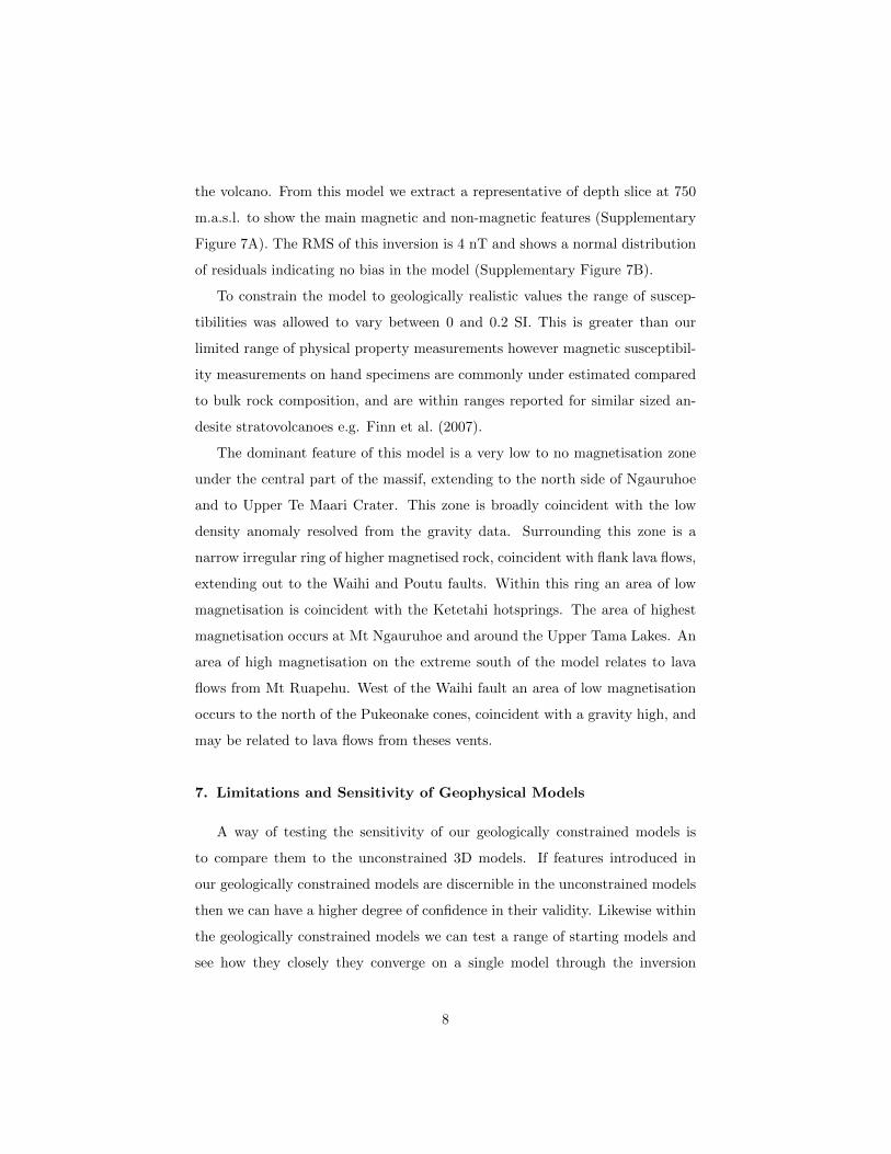
the volcano. From this model we extract a representative of depth slice at 750

m.a.s.l. to show the main magnetic and non-magnetic features (Supplementary

Figure 7A). The RMS of this inversion is 4 nT and shows a normal distribution

of residuals indicating no bias in the model (Supplementary Figure 7B).

To constrain the model to geologically realistic values the range of suscep-

tibilities was allowed to vary between 0 and 0.2 SI. This is greater than our

limited range of physical property measurements however magnetic susceptibil-

ity measurements on hand specimens are commonly under estimated compared

to bulk rock composition, and are within ranges reported for similar sized an-

desite stratovolcanoes e.g. Finn et al. (2007).

The dominant feature of this model is a very low to no magnetisation zone

under the central part of the massif, extending to the north side of Ngauruhoe

and to Upper Te Maari Crater. This zone is broadly coincident with the low

density anomaly resolved from the gravity data. Surrounding this zone is a

narrow irregular ring of higher magnetised rock, coincident with flank lava flows,

extending out to the Waihi and Poutu faults. Within this ring an area of low

magnetisation is coincident with the Ketetahi hotsprings. The area of highest

magnetisation occurs at Mt Ngauruhoe and around the Upper Tama Lakes. An

area of high magnetisation on the extreme south of the model relates to lava

flows from Mt Ruapehu. West of the Waihi fault an area of low magnetisation

occurs to the north of the Pukeonake cones, coincident with a gravity high, and

may be related to lava flows from theses vents.

7. Limitations and Sensitivity of Geophysical Models

A way of testing the sensitivity of our geologically constrained models is

to compare them to the unconstrained 3D models. If features introduced in

our geologically constrained models are discernible in the unconstrained models

then we can have a higher degree of confidence in their validity. Likewise within

the geologically constrained models we can test a range of starting models and

see how they closely they converge on a single model through the inversion

8

process. In each case the RMS misfit of the model indicates all models are

mathematically acceptable representations of the observed data.

The sensitivity of features to a constrained basement depth is judged by if

they extend below basement depths in the unconstrained model, or terminate at

or above the basement in the geologically constrained model. As an example we

compare the iso-surfaces of the low density root imaged beneath Ngauruhoe from

the 3D unconstrained inversion and the geologically constrained model (Supple-

mentary Figure 8A). In the unconstrained inversion the low density root from

Mt Ngauruhoe appears to extend into the basement to a depth of -300 m. In the

geologically constrained model this body is terminated at the basement, how-

ever the low pass filtered data used to construct the basement surface may have

removed the signal of a small low density body close under the basement inter-

face so it is not unreasonable to image the extension of the low density body

into the basement in the unconstrained 3D model using the full wavelength

dataset. This is also feasible when we consider that repeat magmatic intrusion

is likely to leave the basement highly fractured, effectively lowering its density.

Similarly we compare the depth extent of the low magnetic susceptibility body,

associated with the hydrothermal system from unconstrained and geologically

constrained models in Supplementary Figure 8B. In the geologically constrained

model the low susceptibility zone terminates a few hundred metres above the

basement, while in the unconstrained model a larger volume of very low sus-

ceptibility material extends into the basement. This example also illustrates

the geophysical equivalence of a smaller higher susceptibility body and a larger,

lower susceptibility body. The two examples may be taken as end members of

the set of likely models.

Finally we test the sensitivity of our geologically constrained inversion to

the initial starting model used to seed the inversion. In the first model we con-

strained the basement surface to follow the outcrop topography in the Kaimanawa

Ranges and under the TgVM made a flat lying surface at 300 m elevation. In

the second model we used the mapped faults and prior information about their

offsets to construct a geologically feasible starting surface. Geometry inversions

9

on both surfaces using a homogeneous basement density converged on similar

results with the same RMS (1.7 mGal) misfit. While the inversion using the

flat basement surface starting model did not explicitly recreate faulted offsets,

the inverted surface does intersect the locations of the fault traces seen in the

inversion of the faulted starting model. The final basement depths between the

Poutu and Waihi fault zones agree within 100 m (∼10% of the total depth) in

both models, showing that the retrieved shape of the basement surface is mostly

insensitive to the initial starting model.

References

Cassidy, J., Ingham, M., Locke, C.A., Bibby, H., 2009. Subsurface struc-

ture across the axis of the Tongariro Volcanic Centre, New Zealand. Jour-

nal of Volcanology and Geothermal Research 179, 233–240. URL: http:

//linkinghub.elsevier.com/retrieve/pii/S0377027308006100, doi:10.

1016/j.jvolgeores.2008.11.017.

Finn, C.A., Deszcz-Pan, M., Anderson, E.D., John, D.A., 2007. Three-

dimensional geophysical mapping of rock alteration and water content at

Mount Adams, Washington: Implications for lahar hazards. Journal of

Geophysical Research 112, B10204. URL: http://doi.wiley.com/10.1029/

2006JB004783, doi:10.1029/2006JB004783.

Fullagar, P., Pears, G., 2007. Towards geologically realistic inversion. Proceed-

ings of Exploration 07: Fifth Decennial International Conference on Mineral

Exploration , 444–460URL: http://www.dmec.ca/ex07-dvd/E07/pdfs/28.

pdf.

Gottsmann, J., A.G. Camacho, Martı, J., Wooller, L., Fernandez, J., Garcıa,

A., Rymer, H., 2008. Shallow structure beneath the Central Volcanic

Complex of Tenerife from new gravity data: Implications for its evolu-

tion and recent reactivation. Physics of the Earth and Planetary Interi-

10

ors 168, 212–230. URL: http://linkinghub.elsevier.com/retrieve/pii/

S003192010800160X, doi:10.1016/j.pepi.2008.06.020.

Hammer, S., 1939. Terrain Corrections for Gravimeter Stations. Geophysics

4, 184–194. URL: http://dx.doi.org/10.1190/1.1440495, doi:10.1190/

1.1440495.

Hasegawa, T., Yamamoto, A., Kamiyama, H., Nakagawa, M., 2009. Gravity

structure of Akan composite caldera, eastern Hokkaido, Japan: Application

of lake water corrections. Earth, Planets and Space 61, 933–938. URL: http:

//link.springer.com/10.1186/BF03353205, doi:10.1186/BF03353205.

Hautmann, S., Camacho, A.G., Gottsmann, J., Odbert, H.M., Syers, R.T.,

2013. The shallow structure beneath Montserrat (West Indies) from new

Bouguer gravity data. Geophysical Research Letters 40, 5113–5118. URL:

http://doi.wiley.com/10.1002/grl.51003, doi:10.1002/grl.51003.

Nettleton, L.L., 1939. Determination of density for reduction of gravimeter

observations. Geophysics 4. doi:10.1190/1.1437088.

Parasnis, D., 1966. Mining Geophysics. Elsevier, Amsterdam-London-New

York.

11

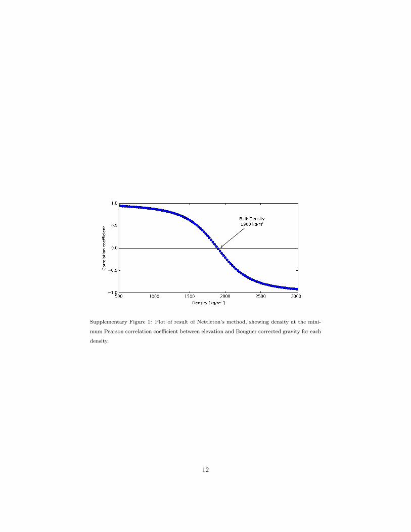
Supplementary Figure 1: Plot of result of Nettleton’s method, showing density at the mini-

mum Pearson correlation coefficient between elevation and Bouguer corrected gravity for each

density.

12

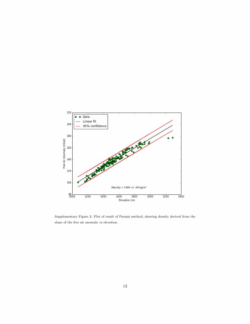
Supplementary Figure 2: Plot of result of Parasis method, showing density derived from the

slope of the free air anomaly vs elevation.

13

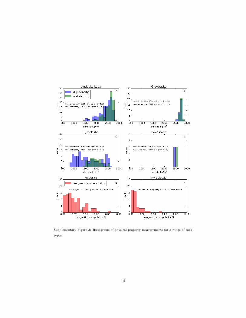
Supplementary Figure 3: Histograms of physical property measurements for a range of rock

types.

14

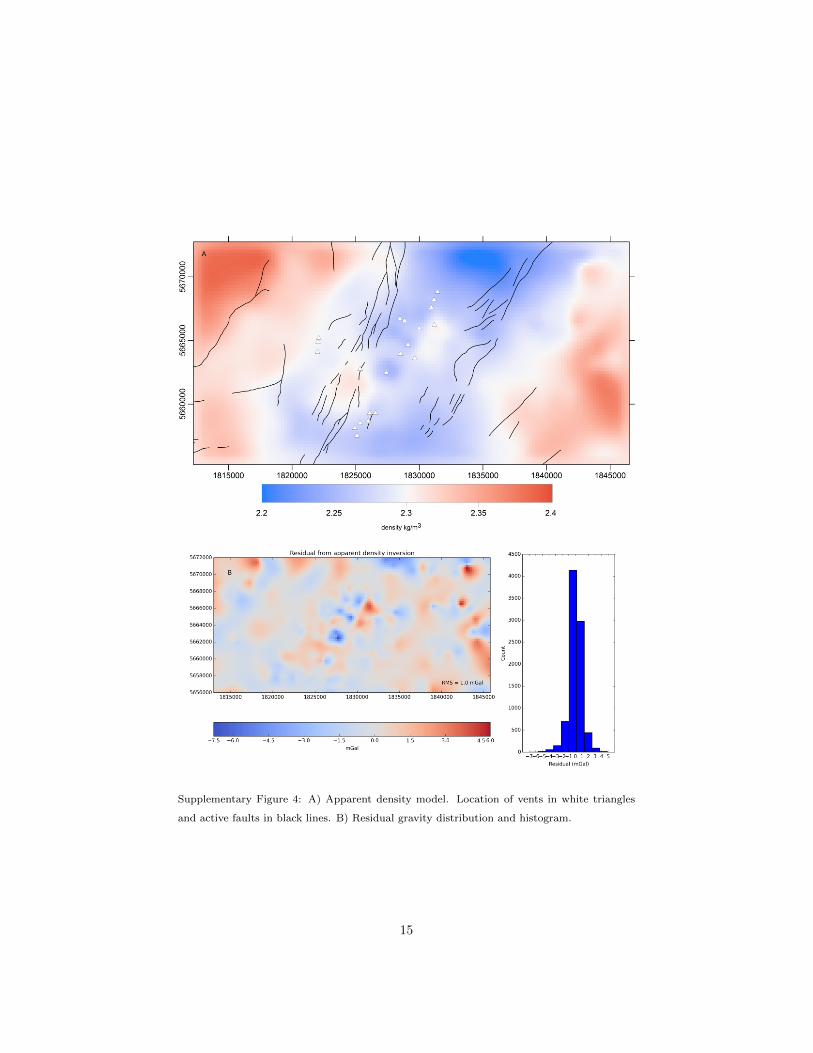
Supplementary Figure 4: A) Apparent density model. Location of vents in white triangles

and active faults in black lines. B) Residual gravity distribution and histogram.

15

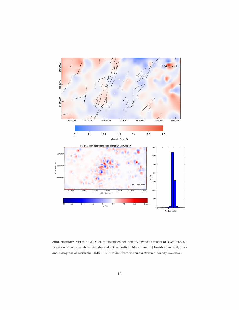
Supplementary Figure 5: A) Slice of unconstrained density inversion model at a 350 m.a.s.l.

Location of vents in white triangles and active faults in black lines. B) Residual anomaly map

and histogram of residuals, RMS = 0.15 mGal, from the unconstrained density inversion.

16

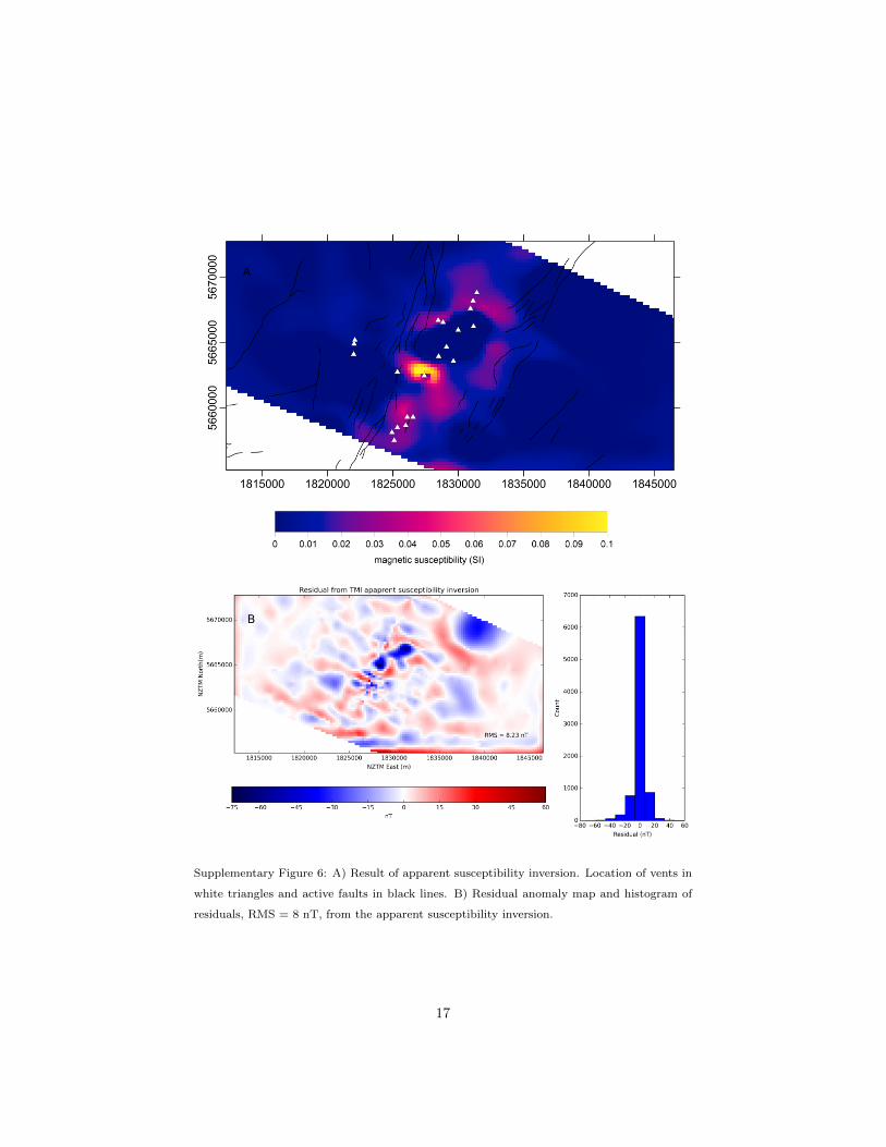
Supplementary Figure 6: A) Result of apparent susceptibility inversion. Location of vents in

white triangles and active faults in black lines. B) Residual anomaly map and histogram of

residuals, RMS = 8 nT, from the apparent susceptibility inversion.

17

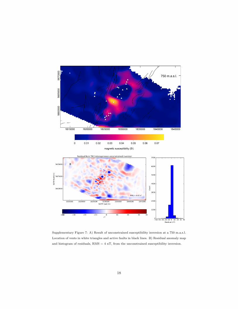
Supplementary Figure 7: A) Result of unconstrained susceptibility inversion at a 750 m.a.s.l.

Location of vents in white triangles and active faults in black lines. B) Residual anomaly map

and histogram of residuals, RMS = 4 nT, from the unconstrained susceptibility inversion.

18

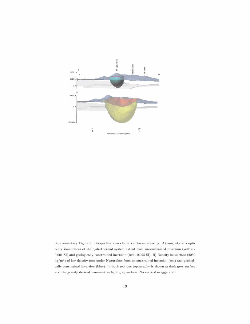
A

0 m

1000 m

2000 m

B

-2500 m

0 m

2000 m

Mt N

gaur

uhoe

Te M

aari

Red

Cra

teri

0 10

Horizontal Distance (km)

S N

Supplementary Figure 8: Perspective views from south-east showing: A) magnetic suscepti-

bility iso-surfaces of the hydrothermal system extent from unconstrained inversion (yellow -

0.001 SI) and geologically constrained inversion (red - 0.025 SI). B) Density iso-surface (2250

kg/m3) of low density root under Ngauruhoe from unconstrained inversion (red) and geologi-

cally constrained inversion (blue). In both sections topography is shown as dark grey surface

and the gravity derived basement as light grey surface. No vertical exaggeration.

19

internal structure and volcanic hazard potential of mt ...16.pdf · internal structure and volcanic...

Documents