international conference on ocean, offshore and arctic ... · formulas based on blevins’ model...

1 Copyright © 2015 by ASME

Proceedings of the 34th

International Conference on Ocean, Offshore and Arctic Engineering OMAE2015

May 31- June 5, 2015, St. John’s, Newfoundland and Labrador, Canada

OMAE2015-41443

HYDRODYNAMIC COEFFICIENT MAPS FOR RISER INTERFERENCE ANALYSIS

Suneel Patel 2H Offshore Inc.

Houston, TX, U.S.A.

Shankar Sundararaman 2H Offshore Inc.

Houston, TX, U.S.A.

Pete Padelopoulos 2H Offshore Inc.

Houston, TX, U.S.A.

Kamaldev Raghavan Chevron Energy Technology

Company Houston, TX, U.S.A.

Metin Karayaka Chevron Energy Technology

Company Houston, TX, U.S.A

Paul Hays Chevron Energy Technology Company

Houston, TX, U.S.A.

Yiannis Constantinides Chevron Energy Technology Company

Houston, TX, U.S.A.

ABSTRACT Riser wake interference analysis is conducted based on

analytical / semi-empirical models such as Blevins’ and Huse’s

models. These models are used for modeling the reduction in

particle flow velocity due to the presence of a cylindrical object

upstream in the flow path. However, these models are often too

conservative and accurate only for circular cylinders. Many top

tensioned risers (TTRs) use vortex induced vibration (VIV)

suppression devices such as strakes or fairings. There is a need

for alternate methods to obtain drag and lift coefficient datasets

for circular cylinders with strakes and fairings. Two such

approaches are to obtain data from Computational Fluid

Dynamics (CFD) simulations or from experimental large-scale

model test data. Interpolation and/or extrapolation methods are

needed to obtain additional data points for global riser finite

element analysis.

This paper presents a methodology to obtain hydrodynamic

coefficients for TTRs with VIV suppression devices. The

proposed methodology uses a combination of empirical

formulas based on Blevins’ model and numerical interpolation

techniques along with experimental tow tank test data and CFD

analysis. The resulting data is then input as user-defined

drag/lift coefficients into a global riser finite element analysis

to obtain a more realistic riser system response.

INTRODUCTION Analytical and semi-empirical models such as Blevins’ and

Huse’s are used for modeling the reduction in current velocity

due to the presence of a cylindrical object upstream in the flow

path. However, these models are often too conservative and

accurate only for circular cylinders. With the presence of VIV

suppression devices on both the upstream and downstream

risers, the risers no longer react as circular cylinders.

Additionally, existing models found in industry guidelines are

based on approximate theoretical models of bare cylinder wake

and nominally checked against small scale tests at low

Reynolds numbers. In actual conditions, the Reynolds number

is sufficiently high for risers fitted with VIV suppression

devices, [3].

Matrices of hydrodynamic drag and lift coefficients are

required for the user-defined wake interference capabilities in

global riser finite element analysis software. These drag

coefficients/drag coefficient factors and lift coefficients vary as

a function of the distance of the downstream riser from the

upstream riser. This variation in drag and lift coefficients due to

the wake effects induced by the upstream riser depend on a

number of factors including the distance between risers, drag

diameter, geometry of the riser (bare, fairing, strake), current

velocity, current direction and Reynolds number.

Learn more at www.2hoffshore.com


Wake Interference Analysis

Wake interference studies between riser pairs are carried

out by assessing a number of factors related to the flow regime,

and the structure. These parameters also include effects of any

VIV suppression devices. The interference between two risers

is evaluated by considering a conservative but realistic wake

model in which the flow behind the upstream cylinder is

modified resulting in reduced velocity downstream. The

downstream structure drag and lift coefficients used to model

this are expressed in terms of the upstream drag diameter

because of the geometric similarity of the wake field behind the

upstream structure.

A simplified riser schematic in profile view of the

upstream-downstream riser pair and the current profile is

illustrated in Figure 1.

Figure 1 – Upstream-Downstream Riser Pair with Current

The plan view of the upstream-downstream riser pair is

illustrated in Figure 2. The drag and lift coefficients are defined

in terms of functions of non-dimensional distances, L/Du and

T/Du, where L and T denote the in-line and transverse distances

between the centerlines of the downstream and upstream

cylinders, and Du is the drag diameter of the upstream cylinder.

When the downstream cylinder is within the wake

generated by the upstream cylinder, it experiences a reduced

drag force due to reduced mean current velocities in the wake

and a lift force as a result of varying pressures across the

cylinder. The drag and lift coefficients for the downstream

cylinder are calculated as functions of its position in the wake

as given in Equation 1 and Equation 2, respectively:

𝐶𝑑 = 𝐶𝑑0λ𝑑(𝐿 𝐷𝑢⁄ , 𝑇 𝐷𝑢⁄ ) = 𝐹𝐷 (1

2𝜌𝑈0

2𝐷𝑢)⁄ (1)

𝐶𝐿 = λ𝐿(𝐿 𝐷𝑢⁄ , 𝑇 𝐷𝑢⁄ ) = 𝐹𝐿 (1

2𝜌𝑈0

2𝐷𝑢)⁄ (2)

where, Cd0 denotes the undisturbed drag coefficients for the

downstream cylinder in the absence of wake effects; λd and λL

are the coefficient factors calculated from the appropriate wake

theory and, FD and FL denote the drag/lift force per unit length

for the downstream riser, U0 is the undisturbed current speed,

Du is the upstream drag diameter and ρ is the fluid density.

As illustrated in Figure 2, the upstream cylinder is at (Xu,

Yu), and the downstream cylinder is at (Xd, Yd). The in-line (L)

and transverse (T) distances can be calculated using Equation 3

and Equation 4, respectively:

𝐿 = 𝑑𝑋 ∗ cos 𝛼 + 𝑑𝑌 ∗ sin 𝛼 (3)

𝑇 = −𝑑𝑋 ∗ sin 𝛼 + 𝑑𝑌 ∗ cos𝛼 (4)

where α is the current direction angle, dX=Xd-Xu and dY=Yd-

Yu.

Figure 2 – Cylinder Model Plan View with Current

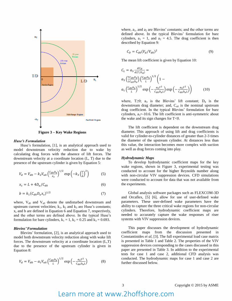
When considering the in-line and transverse distances

between two adjacent risers, there are three key wake regions as

defined in Figure 3. The three key regions are the suction

region, mid-range region and the far-field region. The suction

region corresponds to low in-line and transverse distances. In

the suction region, the drag and lift coefficient factors are

reduced so adjacent risers move closer to each other. The mid-

range region corresponds to in-line and transverse distances

that are typically experienced during 10-year and 100-year

return period environments. The far field region corresponds to

in-line and transverse distances that are great enough to

produce little change in the nominal drag and lift coefficients.

Downstream

Riser

Upstream

Riser

Current

Profile

Current

Direction

dX

dY

Upstream Riser

(Xu,Yu)

Downstream Riser

(Xd,Yd)

T

L

Global

Axes

Current

Direction

Y

X (α=0)

α



Figure 3 – Key Wake Regions

Huse’s Formulation

Huse’s formulation, [1], is an analytical approach used to

model downstream velocity reduction due to wake by

calculating drag forces with the absence of lift forces. The

downstream velocity at a coordinate location (L, T) due to the

presence of the upstream cylinder is given by Equation 5:

𝑉𝑑 = 𝑉𝑑0 − 𝑘2𝑉𝑢0 (𝐶𝑑0𝐷𝑢

𝑥𝑠)1/2

exp (−𝑘3 (𝑇

𝑏)2

) (5)

𝑥𝑠 = 𝐿 + 4𝐷𝑢/𝐶𝑑0 (6)

𝑏 = 𝑘1(𝐶𝑑0𝐷𝑢𝑥𝑠)1/2 (7)

where, Vd0 and Vu0 denote the undisturbed downstream and

upstream current velocities; k1, k2 and k3 are Huse’s constants;

xs and b are defined in Equation 6 and Equation 7, respectively,

and the other terms are defined above. In the typical Huse’s

formulation for bare cylinders, k1 = 1, k2 = 0.25 and k3 = 0.693.

Blevins’ Formulation

Blevins’ formulation, [2], is an analytical approach used to

model both downstream velocity reduction along with wake lift

forces. The downstream velocity at a coordinate location (L,T)

due to the presence of the upstream cylinder is given in

Equation 8:

𝑉𝑑 = 𝑉𝑑0 − 𝑎1𝑉𝑢0 (𝐶𝑑0𝐷𝑢

𝐿)1/2

exp (−𝑎2𝑇

2

𝐶𝑑0𝐷𝑢𝐿) (8)

where, a1, and a2 are Blevins’ constants; and the other terms are

defined above. In the typical Blevins’ formulation for bare

cylinders, a1 = 1, and a2 = 4.5. The drag coefficient is then

described by Equation 9:

𝐶𝐷 = 𝐶𝑑0(𝑉𝑑 𝑉𝑑0⁄ )2 (9)

The mean lift coefficient is given by Equation 10:

𝐶𝐿 = 𝑎3𝑑𝐶𝐷

𝑑(𝑇/𝐷𝑑)=

𝑎3 (𝑇𝐶𝑑0𝐷𝑑

𝐿𝐶𝑢0𝐷𝑢) (

𝐶𝑑0𝐷𝑢

𝐿)1/2

(1 −

𝑎1 (𝐶𝑑0𝐷𝑢

𝐿)1/2

exp (−𝑎2𝑇

2

𝐶𝑑0𝐷𝑢𝐿) exp (−

𝑎2𝑇2

𝐶𝑑0𝐷𝑢𝐿)) (10)

where, T≥0; a3 is the Blevins’ lift constant; Dd is the

downstream drag diameter; and, Cu0 is the nominal upstream

drag coefficient. In the typical Blevins’ formulation for bare

cylinders, a3=-10.6. The lift coefficient is anti-symmetric about

the wake and its sign changes for T<0.

The lift coefficient is dependent on the downstream drag

diameter. This approach of using lift and drag coefficients is

valid for cylinder-to-cylinder distances of greater than 2-3 times

the diameter of the upstream cylinder. At distances less than

this value, the interaction becomes more complex with suction

as well as drag forces coming into play.

Hydrodynamic Maps

To develop hydrodynamic coefficient maps for the key

wake regions, shown in Figure 3, experimental testing was

conducted to account for the higher Reynolds number along

with non-circular VIV suppression devices. CFD simulations

were conducted to account for data that was not available from

the experiments.

Global analysis software packages such as FLEXCOM-3D

and Orcaflex, [5] [6], allow for use of user-defined wake

parameters. These user-defined wake parameters have the

ability to capture the three critical wake regions for non-circular

cylinders. Therefore, hydrodynamic coefficient maps are

needed to accurately capture the wake responses of riser

systems with VIV suppression devices.

This paper discusses the development of hydrodynamic

coefficient maps from the discussion presented in

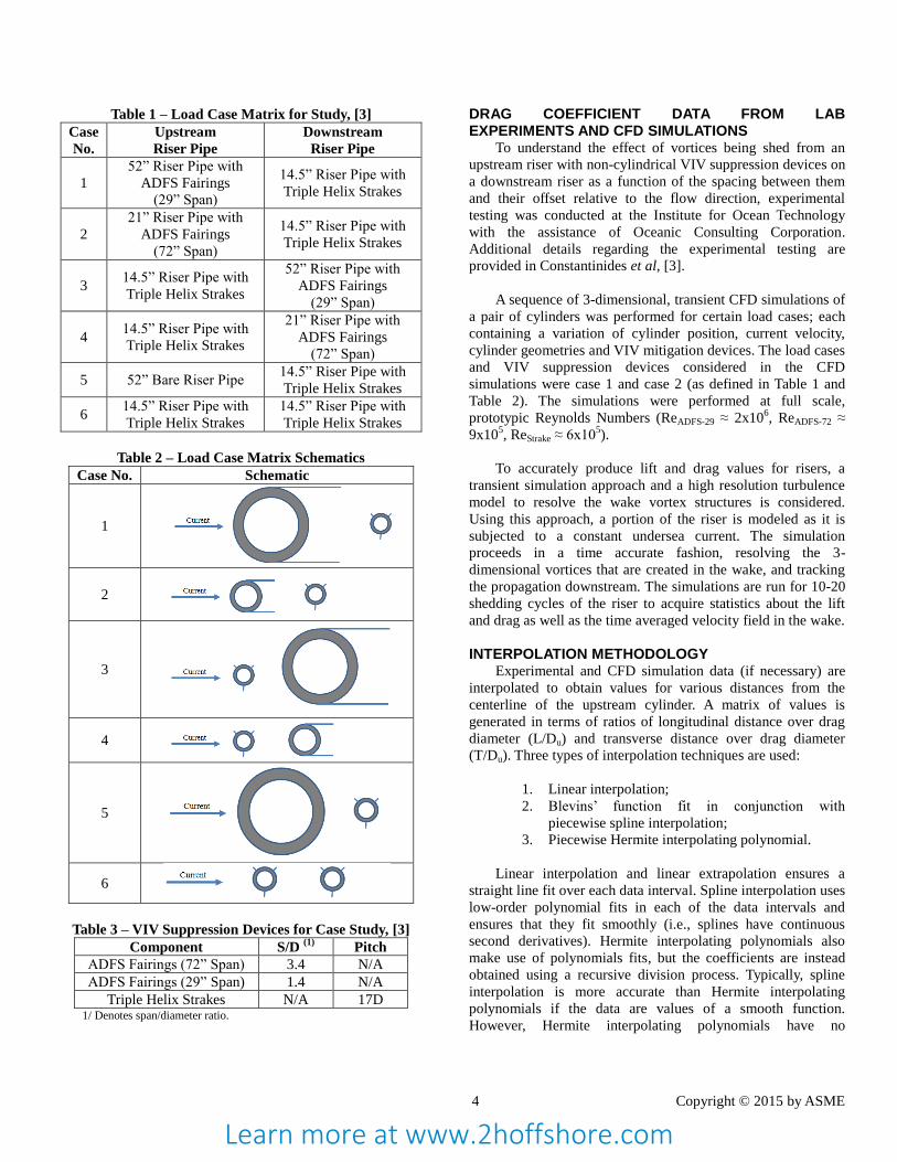
Constantinides et al, [3]. The full experimental load case matrix

is presented in Table 1 and Table 2. The properties of the VIV

suppression devices corresponding to the cases discussed in this

paper are presented in Table 3. In addition to the experimental

tests for case 1 and case 2, additional CFD analysis was

conducted. The hydrodynamic maps for case 1 and case 2 are

further discussed below.



Table 1 – Load Case Matrix for Study, [3]

Case

No.

Upstream

Riser Pipe

Downstream

Riser Pipe

1

52” Riser Pipe with

ADFS Fairings

(29” Span)

14.5” Riser Pipe with

Triple Helix Strakes

2


ADFS Fairings

(72” Span)



3 14.5” Riser Pipe with



ADFS Fairings

(29” Span)




ADFS Fairings

(72” Span)

5 52” Bare Riser Pipe 14.5” Riser Pipe with






Table 2 – Load Case Matrix Schematics

Case No. Schematic

1

2

3

4

5

6

Table 3 – VIV Suppression Devices for Case Study, [3]

Component S/D (1)

Pitch

ADFS Fairings (72” Span) 3.4 N/A

ADFS Fairings (29” Span) 1.4 N/A

Triple Helix Strakes N/A 17D 1/ Denotes span/diameter ratio.

DRAG COEFFICIENT DATA FROM LAB EXPERIMENTS AND CFD SIMULATIONS

To understand the effect of vortices being shed from an

upstream riser with non-cylindrical VIV suppression devices on

a downstream riser as a function of the spacing between them

and their offset relative to the flow direction, experimental

testing was conducted at the Institute for Ocean Technology

with the assistance of Oceanic Consulting Corporation.

Additional details regarding the experimental testing are

provided in Constantinides et al, [3].

A sequence of 3-dimensional, transient CFD simulations of

a pair of cylinders was performed for certain load cases; each

containing a variation of cylinder position, current velocity,

cylinder geometries and VIV mitigation devices. The load cases

and VIV suppression devices considered in the CFD

simulations were case 1 and case 2 (as defined in Table 1 and

Table 2). The simulations were performed at full scale,

prototypic Reynolds Numbers (ReADFS-29 ≈ 2x106, ReADFS-72 ≈

9x105, ReStrake ≈ 6x10

5).

To accurately produce lift and drag values for risers, a

transient simulation approach and a high resolution turbulence

model to resolve the wake vortex structures is considered.

Using this approach, a portion of the riser is modeled as it is

subjected to a constant undersea current. The simulation

proceeds in a time accurate fashion, resolving the 3-

dimensional vortices that are created in the wake, and tracking

the propagation downstream. The simulations are run for 10-20

shedding cycles of the riser to acquire statistics about the lift

and drag as well as the time averaged velocity field in the wake.

INTERPOLATION METHODOLOGY Experimental and CFD simulation data (if necessary) are

interpolated to obtain values for various distances from the

centerline of the upstream cylinder. A matrix of values is

generated in terms of ratios of longitudinal distance over drag

diameter (L/Du) and transverse distance over drag diameter

(T/Du). Three types of interpolation techniques are used:

1. Linear interpolation;

2. Blevins’ function fit in conjunction with

piecewise spline interpolation;

3. Piecewise Hermite interpolating polynomial.

Linear interpolation and linear extrapolation ensures a

straight line fit over each data interval. Spline interpolation uses

low-order polynomial fits in each of the data intervals and

ensures that they fit smoothly (i.e., splines have continuous

second derivatives). Hermite interpolating polynomials also

make use of polynomials fits, but the coefficients are instead

obtained using a recursive division process. Typically, spline

interpolation is more accurate than Hermite interpolating

polynomials if the data are values of a smooth function.

However, Hermite interpolating polynomials have no



overshoots and have fewer oscillations if the data is not smooth

(non-monotonic).

Additionally, the Blevins’ function is used to fit a bulk of

the data points along the transverse direction. The Blevins’

function is also incorporated in a piece-wise sense; i.e.,

different sets of Blevins’ coefficients are used to fit pairs of data

points. The Blevins’ coefficients used to generate the tables are

based on the nominal drag coefficients and diameters used in

the respective CFD simulation/laboratory experiment. Two sets

of Blevins’ functions are used, depending on whether the drag

coefficients or lift coefficients are generated.

Approach to Extract Drag Coefficients

A four step process is used to extract the drag coefficients

for all cases presented in Table 1 and Table 2. The steps to

generate the drag coefficients are provided using case 1 as an

example. The contour plots of drag coefficient ratios are

provided for case 1 and case 2 to show how these cases differ.

The steps used to generate the drag coefficients are as

follows:

1. The drag coefficient ratios are fitted along the in-line

longitudinal direction as shown in Figure 4 for case 1.

A piecewise cubic Hermite interpolating polynomial is

used to interpolate or extrapolate data based on each

set of experimental/CFD simulation data points.

2. The Blevins’ function is used to generate data and fit

the data along the transverse direction (0, T1/Du, T2/Du,

Tn/Du), where Tn/Du refers to the ratio of the transverse

distance of the nth data point to the upstream riser drag

diameter. This fit is carried out along each set of data

points obtained in the in-line longitudinal direction (0,

L1/Du, L2/Du, Lm/Du), where Lm/Du refers to the ratio

of the longitudinal distance of the mth data point to the

upstream riser drag diameter. Wherever the Blevins’ fit

does not pass through all the data points (typically in

the suction region), a combination cubic spline and

piecewise cubic Hermite interpolating polynomial fit

is used to ensure that the final fit passes through all the

data points obtained. Step 2 is illustrated in Figure 5.

3. The drag coefficient ratios are then fitted along the in-

line longitudinal direction (0, L1/Du, L2/Du, etc.) as

illustrated in Figure 6. A combination of linear

interpolation (in the suction region) and piecewise

cubic Hermite interpolating polynomial (when the

distance between the two risers is great enough) is

used to extrapolate the remaining data points along the

longitudinal direction (0, L1/Du, L2/Du, etc.).

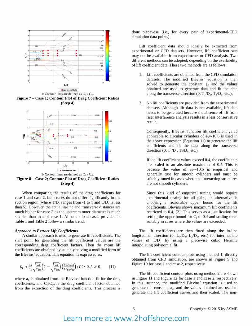
4. Steps 1-3 are repeated along every longitudinal and

transverse line of interest to generate a contour plot.

This data, including the illustrations in Figure 7 and

Figure 8, is generated with a longitudinal spacing of

0.05 between L=Du and L=2Du, 0.25 between L=2Du

and L=5Du, and 0.50 greater than L=5Du and a

transverse spacing of 0.05 between T=0 and T=Du,

and 0.50 greater than T= Du. This spacing is adopted

because most global riser analysis software, such as

FLEXCOM-3D and Orcaflex, [5] [6], require fine

spacing when the two cylinders are in close proximity.

Figure 4 – Case 1; Drag Coefficient Ratio Fitted along

Longitudinal Direction (T/Du=0) (Step 1)


Transverse Direction (L/Du=0) (Step 2)


Longitudinal Direction (T/Du=0) (Step 3)

Experimental Data Hermite Polynomial FitBlevins Eq. Huse Eq.

0 5 10 15 20 25-0.2

0

0.2

0.4

0.6

0.8

1

L/D-upstream

Cd

-do

wn

str

ea

m/

Cd

-no

min

al

Drag Ratio Fitted along Longitudinal Direction (Buoyant Fairing-Strake)

0 5 10 15 20 25-0.2

0

0.2

0.4

0.6

0.8

1

L/D-upstream

Cd

-do

wn

str

ea

m/C

d-n

om

ina

l


Experimental Data Blevins Eq./Spline FitBlevins Eq. Huse Eq.

0 0.5 1 1.5 2 2.5 3 3.5 4-0.2

0

0.2

0.4

0.6

0.8

1

T/D-upstream

Cd

-do

wn

str

ea

m/

Cd

-no

min

al

Drag Ratio Fitted along Transverse Direction (Buoyant Fairing-Strake)

0 0.5 1 1.5 2 2.5 3 3.5 4-0.2

0

0.2

0.4

0.6

0.8

1

T/D-upstream

Cd

-do

wn

str

ea

m/

Cd

-no

min

al

Drag Ratio Fitted along Transverse Direction (Buoyant Fairing-Strake)

Piecewise cubic spline+cubic Hermite

interpolating polynomial fit

(Suction Region)

Piecewise Blevins fit

Experimental Data Hermite Polynomial/Linear FitBlevins Eq. Huse Eq.

0 5 10 15 20 25-0.2

0

0.2

0.4

0.6

0.8

1

L/D-upstream

Cd

-do

wn

str

ea

m/

Cd

-no

min

al


0 5 10 15 20 25-0.2

0

0.2

0.4

0.6

0.8

1

L/D-upstream

Cd

-do

wn

str

ea

m/C

d-n

om

ina

l


Linear Fit

(Suction Region)

Piecewise Cubic Hermite

Interpolating Polynomial Fit



1/ Contour lines are defined as Cd, / Cd0.

Figure 7 – Case 1; Contour Plot of Drag Coefficient Ratios

(Step 4)

1/ Contour lines are defined as Cd, / Cd0.

Figure 8 – Case 2; Contour Plot of Drag Coefficient Ratios

(Step 4)

When comparing the results of the drag coefficients for

case 1 and case 2, both cases do not differ significantly in the

suction region (where T/Du ranges from -1 to 1 and L/Du is less

than 5). However, the actual in-line and transverse distances are

much higher for case 2 as the upstream outer diameter is much

smaller than that of case 1. All other load cases provided in

Table 1 and Table 2 follow a similar trend.

Approach to Extract Lift Coefficients

A similar approach is used to generate lift coefficients. The

start point for generating the lift coefficient values are the

corresponding drag coefficient factors. Then the mean lift

coefficients are obtained by suitably solving a modified form of

the Blevins’ equation. This equation is expressed as:

𝐶𝑙 ≈𝑎3

𝑎1√

𝐶𝑑

𝐶𝑑0(1 − √

𝐶𝑑

𝐶𝑑0) (

𝑇𝑐𝑑0𝐷𝑑

𝐿𝑐𝑢0𝐷𝑢) ; 𝑇 ≥ 0, 𝐿 > 0 (11)

where a1 is obtained from the Blevins’ function fit for the drag

coefficients, and Cd/Cd0 is the drag coefficient factor obtained

from the extraction of the drag coefficients. This process is

done piecewise (i.e., for every pair of experimental/CFD

simulation data points).

Lift coefficient data should ideally be extracted from

experimental or CFD datasets. However, lift coefficient sets

may not be available from experiments or CFD analysis. Two

different methods can be adopted, depending on the availability

of lift coefficient data. These two methods are as follows:

1. Lift coefficients are obtained from the CFD simulation

datasets. The modified Blevins’ equation is then

solved to generate the constant, a3 and the values

obtained are used to generate data and fit the data

along the transverse direction (0, T1/Du, T2/Du, etc.).

2. No lift coefficients are provided from the experimental

datasets. Although lift data is not available, lift data

needs to be generated because the absence of lift from

riser interference analysis results in a less conservative

result.

Consequently, Blevins’ function lift coefficient value

applicable to circular cylinders of a3=-10.6 is used in

the above expression (Equation 11) to generate the lift

coefficients and fit the data along the transverse

direction (0, T1/Du, T2/Du, etc.).

If the lift coefficient values exceed 0.4, the coefficients

are scaled to an absolute maximum of 0.4. This is

because the value of a3=-10.6 is empirical and

generally true for smooth cylinders and must be

suitably tuned in cases where the interacting structures

are not smooth cylinders.

Since this kind of empirical tuning would require

experimental testing for all pairs, an alternative is

choosing a reasonable upper bound for the lift

coefficients. Blevins shows maximum lift coefficients

restricted to 0.4, [2]. This serves as a justification for

setting the upper bound for Cl to 0.4 and scaling them

suitably in cases where the values are exceeded.

The lift coefficients are then fitted along the in-line

longitudinal direction (0, L1/Du, L2/Du, etc.) for intermediate

values of L/Du by using a piecewise cubic Hermite

interpolating polynomial fit.

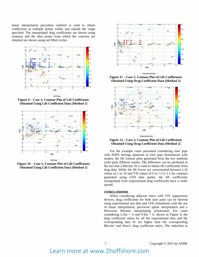
The lift coefficient contour plots using method 1, directly

obtained from CFD simulation, are shown in Figure 9 and

Figure 10 for case 1 and case 2, respectively.

The lift coefficient contour plots using method 2 are shown

in Figure 11 and Figure 12 for case 1 and case 2, respectively.

In this instance, the modified Blevins’ equation is used to

generate the constant, a3, and the values obtained are used to

generate the lift coefficient curves and then scaled. The non-

Experimental Data

0.10.20.30.40.5

0.6 0.75

0.75

0.85

0.85

0.85

0.85

0.850.85

0.9

0.9

0.9

0.9

0.95

0.95

0.95

0.95

0.99

0.9

9

0.99

0.9

9

0.99

99

0.9999

L/D

T/

DDrag Coefficient Ratio (Buoyant Fairing-Strake)

0 5 10 15-5

-4

-3

-2

-1

0

1

2

3

4

5

0

0.1

0.2

0.3

0.4

0.5

0.6

0.7

0.8

0.9

1

Experimental Data

0.75

0.85

0.85

0.9

0.9

0.90.9

0.95 0.95 0.95

0.95 0.95 0.95

0.950.950.95 0.95

0.99

0.99 0.99 0.99

0.99

0.99 0.99 0.99

0.9999

0.9999 0.9999 0.9999

0.9999

0.9999 0.9999 0.9999

L/D

T/

D

Drag Coefficient Ratio (Non-Buoyant Fairing-Strake)

0 5 10 15 20 25-15

-10

-5

0

5

10

15

0.75

0.8

0.85

0.9

0.95



linear interpolation procedure outlined is used to obtain

coefficients at multiple points within and outside the range

specified. The interpolated drag coefficients are shown using

contours and the data points from which the contours are

obtained are shown using red filled circles.

Figure 9 – Case 1; Contour Plot of Lift Coefficients

Obtained Using Lift Coefficient Data (Method 1)


Obtained Using Lift Coefficient Data (Method 1)


Obtained Using Drag Coefficient Data (Method 2)


Obtained Using Drag Coefficient Data (Method 2)

For the example cases presented considering riser pipe

with ADFS fairings upstream to riser pipe downstream with

strakes, the lift contour plots generated from the two methods

yield quite different results. The difference can be attributed to

the fact that a Blevins’ fit is used to obtain lift coefficients from

drag data. While the lift forces are concentrated between L/D

values of 1 to 10 and T/D values of 0 to +1.5/-1.5 for contours

generated using CFD data points, the lift coefficients

extrapolated from experimental drag coefficients have a wider

spread.

CONCLUSIONS When considering adjacent risers with VIV suppression

devices, drag coefficients for both riser pairs can be derived

using experimental test data and CFD simulations with the use

of linear interpolation, piecewise spline interpolation and a

Piecewise Hermite interpolating polynomial. For cases

considering L/Du > 4 and T/Du = 0, shown in Figure 4, the

drag coefficient ratios for all the experimental data and the

corresponding data fit are higher than the corresponding

Blevins’ and Huse’s drag coefficient ratios. The reduction in

CFD Data

-0.5-0.4

-0.4

-0.3

-0.3

-0.3

-0.25

-0.25 -0.25

-0.2

-0.2

-0.2

-0.1

-0.1

-0.1

-0.1

-0.01-0.01

-0.01

-0.0

1

-0.01 -0.01 -0.01-0.01-0.01 -0.01 -0.01-0.01

-0.0001-0.0001

-0.0

001

-0.0001

-0.0

001

-0.0001 -0.0001

-0.0

001

000

0

00 0 00 0.00010.00010.00010.0001

0.0

001

0.0001

0.0

001

0.0001

0.010.010.01

0.0

1

0.01

0.010.01

0.010.1

0.1

0.1

0.1

0.2

0.2

0.2

0.250.25

0.25

0.3

0.3

0.3

0.4

0.4

0.5

L/D

T/

D

Lift Coefficient (Buoyant Fairing-Strake)

0 5 10 15 20 25-5

-4

-3

-2

-1

0

1

2

3

4

5

-0.5

-0.4

-0.3

-0.2

-0.1

0

0.1

0.2

0.3

0.4

0.5

CFD Data

-0.5-0.4

-0.3

-0.3

-0.25

-0.25

-0.2

-0.2

-0.2

-0.1-0.1

-0.1

-0.1-0.1-0.1

-0.01-0.01

-0.01

-0.0

1

-0.01 -0.01 -0.01-0.01-0.01-0.01 -0.01 -0.01 -0.01

-0.0001-0.0001

-0.0001

-0.0

001

-0.0001 -0.0001 -0.0001

000

0

0 0 0 00.00010.00010.0001

0.0

00

1

0.0001

0.0001 0.0001

0.010.010.01

0.0

1

0.010.01 0.01

0.10.1

0.1

0.10.1

0.1

0.2

0.20.2

0.25

0.25

0.30.3 0.4

0.5

L/D

T/D

Lift Coefficient (Slick Fairing-Strake)

0 5 10 15 20 25-5

-4

-3

-2

-1

0

1

2

3

4

5

-0.5

-0.4

-0.3

-0.2

-0.1

0

0.1

0.2

0.3

0.4

0.5

Experimental Data

-0.2

-0.1-0.1

-0.1

-0.01

-0.01

-0.01

-0.0

1

-0.01 -0.01 -0.01

-0.0001-0.0001

-0.0

001

-0.0001-0.0001 -0.0001 -0.0001

-0.0001

000

0

0 0 0 0

0

0.00010.00010.0001

0.0001

0.0001

0.0001 0.0001

0.0001

0.010.010.01

0.0

1

0.0

1

0.010.01

0.01

0.10.1

0.1

0.1 0.2

L/D

T/D

Lift Coefficient (Drag Extrap.) (Buoyant Fairing-Strake)

0 5 10 15 20 25-5

-4

-3

-2

-1

0

1

2

3

4

5

-0.2

-0.15

-0.1

-0.05

0

0.05

0.1

0.15

0.2

Experimental Data

-0.75

-0.75

-0.5

-0.5

-0.5

-0.4

-0.4

-0.4

-0.3

-0.3

-0.3

-0.3

-0.25-0.25

-0.25

-0.25

-0.25

-0.2-0.2

-0.2

-0.2

-0.2

-0.1

-0.1

-0.1

-0.1-0.1

-0.1

-0.01-0.01-0.01

-0.0

1

-0.01 -0.01

-0.0001-0.0001-0.0001

-0.0

001

-0.0001 -0.0001

000

0

0 0 00.00010.00010.0001

0.0

001

0.0001 0.0001

0.010.010.01

0.01

0.01 0.01 0.01

0.10.1

0.1

0.1

0.1

0.1

0.20.2

0.2

0.2

0.2

0.250.25

0.25

0.25

0.25

0.3

0.3

0.3

0.3

0.4

0.4

0.4

0.5

0.5

0.50.75

0.75

L/D

T/

D

Lift Coefficient (Drag Extrap.) (Non-Buoyant Fairing-Strake)

0 5 10 15 20 25-5

-4

-3

-2

-1

0

1

2

3

4

5

-0.6

-0.4

-0.2

0

0.2

0.4

0.6



drag coefficient will affect the clearance between adjacent riser

pairs.

Lift coefficients can also be derived from either drag data

or CFD simulations using the modified Blevins’ equation

provided by Equation 10. As the validity of lift coefficients

generated from either method is somewhat debatable, the more

conservative of the two techniques, evaluated on a case by case

basis, should be used when evaluating the global riser system

response.

The resulting drag and lift coefficients are then input as

user-defined drag and lift coefficients into a global riser finite

element analysis to obtain a more realistic riser system

response. Further discussion regarding the use of inputs to user-

defined drag and lift coefficients and its effect on riser-to-riser

clearance is provided by Sundararaman et al, [4].

NOMENCLATURE ADFS AIMS Dual Fin Splitter

CFD Computation Fluid Dynamics

TTR Top Tensioned Riser

VIV Vortex Induced Vibration

REFERENCES [1] Huse,.E., - “Experimental Investigation of Deep Sea

Riser Interaction”; OTC1996-8070; May 1996.

[2] Blevins, R.D. – “Forces on and Stability of a

Cylinder in a Wake”; J. OMAE, 127, 39-45, 2005.

[3] Constantinides, Y., Raghavan, K., Karayaka, M.,

Spencer, D., - “Tandem Riser Hydrodynamic Tests at

Prototype Reynolds Number”, OMAE2013-10951,

2013.

[4] Sundararaman, S., Saldana, D., Patel, S., Andrew, B.,

Padelopoulos, P., Karayaka, M., Raghavan, K., Hays,

P., - “Interference Assessment between Top

Tensioned Risers for Tension Leg Platform Using a

Simplified Screening Approach”, OMAE2015-41466,

2015.

[5] Marine Computational Services (MCS) –

“FLEXCOM-3D Three-Dimensional Nonlinear Time

Domain Offshore Analysis Software.” Version 7.10,

2011.

[6] Orcina Ltd. – “ORCAFLEX User Manual.” Version

9.3a, 2009.


international conference on ocean, offshore and arctic ... · formulas based on blevins’ model...

Documents