International Economic Geography –Transport infrastructure investment

dr hab. Bart Rokicki

Chair of Macroeconomics and Foreign Trade TheoryFaculty of Economic Sciences, University of Warsaw

Public infrastructure investment

• Public infrastructure investment has been widely used as one of the main tools of regional policy

• Big, multiannual infrastructural investment programs already in the 1950s (e.g., Cassa per il Mezzogiorno in Italy)

• However, in Europe major programs under the EU Cohesion Policy since the late 1980s

• Currently other big economies also use such a policies as a part of its development programmes (e.g., China, India)

• Problems with cost overruns and delays (e.g., Flyvbjerg et al., 2002)

• Unclear long-term macroeconomic impacts

What does theory suggest?

• Neo-classical theory suggests that public infrastructure investment may speed-up convergence process through capital accumulation (although not necessarily improve long-term economic growth).

• More positive outcome if we assume that it improves overall productivity – see Solow model!

• New economic geography indicates that change in the transport costs may seriously influence spatial allocation of economic activity. Hence, actually investment in transport infrastructure in less developed areas could harm their long-run economic growth

• Which one is right?

Possible analytical approaches

There are three main approaches that deal with the impact of transport infrastructure on regional economic development.

The Cost-Benefit Analysis (CBA) is probably the most widely used of the three potential approaches. However, most CBA studies are both limited in scope and partial in nature (the scope is usually microeconomic).

The macroeconomic approach that follows paper by Aschauer(1989) considers general productivity effects of infrastructure. Usually, it simply treats public infrastructure as a production factor in standard neoclassical production function.

The second macroeconomic approach links transportation networks and computable general equilibrium (CGE) models.

Finally, there are at least several papers that try to analyze the relationship between transport infrastructure and regional development applying structural equations framework (e.g. Duranton and Turner, 2012).

General productivity effects

• Most of econometric based papers follow the approach by Aschauer(1989) and analyze general productivity effects of infrastructure.

• In her study, Aschauer (1989) used Cobb-Douglas production function which in logs took form of:

where A is TFP index purged of the influence of government capital stock, K private capital stock, L labour force and G is government capital stock

• Aschauer (1989) finds surprisingly high production elasticity for public capital which seems implausible. As Gramlich (1994) shows if we apply the elasticity from Aschauer’s study it turns out that the marginal product of government capital has to be 100% or more yearly. Holtz-Eakin (1988) and Munnell (1990a) received similar results following similar framework.

GcLbKaAQ lnlnlnlnln

General productivity effects (2)

• In general, the existing literature shows that there is a certain degree of complementarity between public and private investment. However, several studies show that, while controlling for some unobserved region-specific effects, transport infrastructure investment can have in fact a negligible impact on private sector productivity (e.g., Holtz-Eakin, 1994; Evans and Karras, 1994; Crihfield and Panggabean, 1995).

• Here, controversies arise in terms of the public infrastructure definition, data used (time series, cross-section, panel data), econometric specifications (e.g. problems concerning dynamics, co-integration and causality) or the spatial level (national versus regional data).

• Also, the interpretation of results can be difficult due to the fact that short-term expenditure effects are confused with long-run productivity effects (e.g., Sturm et al., 1999).

• Furthermore, the literature shows that the change in accessibility may have a different impact on different locations. In this sense the impact of infrastructure investment is nonlinear (e.g., Boarnet, 1996, 1998).

Accessibility and productivity

• The change in accessibility and thus transportation costs may lead to significant relocation of economic activity. This in turn would improve overall productivity level due to the change in the labor market. First, if journey times are reduced workers may be more willing to work longer hours. Second, the enlarged labor market will enable workers to search for more productive jobs within the agglomeration due to the existence of scale economies (e.g., Venables, 2007).

• Positive impact of improved accessibility on productivity could be also expected at the level of firms. Here, in general a decrease in transport costs should induce a tendency to substitute into a more transport intensive way of production.

• Moreover, investment in transport infrastructure that improves interregional or international accessibility may additionally improve local productivity due to possible import of knowledge (e.g., Karlsson et al., 2006). On the other hand emigration of skilled labor or increased competition from abroad could have completely opposite effect.

Accessibility and production

• One of the common problems concerning studies on general productivity effects relates to the definition of the transport infrastructure variable. Here, the cost of construction per kilometer may vary considerably both because of the nature of the project and differences between regions in terms of landscape.

• Hence, changes in capital stock values must be considered as rather poor indicators of the services provided by infrastructure networks. From this point of view, several authors suggest the introduction, into the production function approach, of the accessibility concept, commonly used in transportation research.

• Until very recently, the only papers that try to directly deal with the above issue refer to the case of Sweden. Here we can find papers by Forslund and Johansson (1995), Karlsson et al. (2008) or Ejermo and Gråsjö (2011). First papers to formally assess the impact of accessibility on productivity in different theoretical frameworks by Rokicki and Stępniak (2018) and Rokicki et al. (2020).

• Relatively few studies tried to empirically verify the impact of accessibility improvement on regional employment

• In the case of the US, Islam (2003) show positive but highly localized geographically effect of the Appalachian Development Highway program on local employment. Duranton and Turner (2012) find that a 10% increase in a city's initial stock of highways causes about a 1.5% increase in its employment over 20 year period.

• In Europe, Dodgson (1974) or Botham (1980) report positive relationship between accessibility and local employment growth in the UK. Linneker and Spence (1996) assess the impact of the M25 London orbital motorway construction on regional employment growth. They find that accessibility is likely to be dual-causal and bilateral in its impact.

• All of the above studies use road length as a proxy for accessibility.

Accessibility and employment

• Most of the studies related to accessibility issue apply the potential accessibility measure. The measure combines two critical elements of accessibility, namely land use and transportation (Geurs and van Wee, 2004).

• It usually uses population as a proxy of destination attractiveness (holding itconstant), travel time as an impedance component and a negative exponential as a distance decay function. The accessibility value for unit i is expressed by the following formula:

where Ai is accessibility of unit i, Mj represents attractiveness of the destination j (i.e. population) and tij is a travel time between i and j. Following the ‘half-life’ approach (Östh et al., 2014), β parameters enforce the assumption that the destination attractiveness decreases by half at the observed median travel time and correspond to the typical trip duration of 120 and 50 minutes, respectively.

Accessibility measure

High-speed road investment – the case of Poland

Since 2004, as a result of the EU accession, Poland has experienced massive improvement in road infrastructure. Due to the fact that Poland received financial support from the Cohesion Fund special stress was put on development of motorways and expressways.

Actually, high-speed roads network was basically non-existing before 2004, as it consisted of less than 500 km of separate, unconnected sections. In 2015, already over 3000 km of high-speed roads were connecting most important Polish cities.

Here, 48 projects were completed with the financial support from the EU. As claimed by Rosik et al. (2015) the EU support accounts for around 68% of overall projects costs.

Location of newly costructed roads in Poland between 2004 and 2014

Relative change in accessibility between 2004 and 2014

• We rely on neoclassical Cobb-Douglas aggregate regional production function with the Hicks-neutral technology (e.g. Fernald, 1999):

• However, instead of using the levels we estimate the changes.

• By taking logs and differentiating, the change in output in region i attime t can be expressed as:

• where the lower case letters stand for the log of variables.

• In the case of employment we estimate labor demand function thatdepends on the destruction rate, the growth rate of labour demand and the adjustment costs. It is given by:

The impact of transport infrastructure investment on Polish economy

We face potential endogeneity issue in the case of accessibility variable. If this problem is real then our estimation results will be biased.

In order to deal with the problem we follow Duranton and Turner (2012) and construct three different instruments for accessibility

• First of them relies on the planned motorways in 1945

• Second refers to planned express roads from 1963

• Finally, we also use a plan of main train routes from 1952

Endogeneity issue

Instrument 1 (1945)

• We construct a cross-section database for the Polish NUTS3 level regions and LAU1 areal units covering the 2004-2014 period.si

• The accessibility variable is calculated using the travel speed model based on14 pre-defined categories of road in Poland. The population data come from the Central Statistical Office.

• The data on regional value added, wages, employment and fixed capital for the NUTS3 regions comes from the Local Data Bank. We use the data for enterprises only - this way we cover the market part of the economy.

• In the case of the LAU1 areas we rely on experimental estimations of regional value added following approach by Ciołek and Brodnicki(2016)

• The data on instrument was calculated using approximations from particular road and rail plans.

The data

Results – instrumental variables

(1) (2)

VARIABLES Model Model

Delta accessibility 0.484 0.512(0.488) (0.523)

Delta capital 0.143** 0.392***(0.065) (0.060)

Delta employment 0.510***(0.109)

Delta wages -0.509(0.340)

Log income 0.397***(0.089)

Log wages -0.351**(0.159)

Log employment -0.379***(0.084)

Constant 0.152* 3.397***(0.092) (1.177)

Observations 72 72R-squared 0.52 0.53Adj. R-squared 0.50 0.49

Sargan Statistic (overidentification) 3.841 0.897Chi-sq (2) P-val 0.147 0.639Durbin-Wu-Hausman (endogeneity) 0.837 0.178Chi-sq (1) P-val 0.360 0.673

Notes: 2SLS estimation. *, ** and *** represent significance at 10%, 5% and 1%,respectively.

Our results suggest the lack of endogeneity (see tests).

Results – NUTS3 regions

(1) (2) (3) (4) (5) (6)VARIABLES Model Model Model Model Model Model

Delta accessibility 0.081 1.076 0.305* 1.276(interregional) (0.154) (0.904) (0.162) (0.867)Delta accessibility square -2.487 -2.424(interregional) (2.179) (2.218)Delta accessibility -0.001 0.316*(international) (0.180) (0.165)Delta capital 0.131** 0.133** 0.129** 0.398*** 0.392*** 0.396***

(0.063) (0.063) (0.064) (0.070) (0.070) (0.073)Delta employment 0.551*** 0.541*** 0.559***

(0.086) (0.089) (0.085)Delta wages -0.489 -0.460 -0.451

(0.295) (0.299) (0.281)Log income 0.394*** 0.391*** 0.362***

(0.105) (0.106) (0.113)Log wages -0.341** -0.322** -0.307**

(0.145) (0.146) (0.142)Log employment -0.372*** -0.375*** -0.340***

(0.102) (0.104) (0.109)Constant 0.227*** 0.138 0.242*** 3.303*** 3.123*** 2.970***

(0.032) (0.084) (0.041) (1.068) (1.085) (1.073)

Observations 72 72 72 72 72 72R-squared 0.56 0.57 0.56 0.54 0.55 0.54Adj. R-squared 0.54 0.54 0.54 0.50 0.50 0.50Notes: Robust standard errors in parentheses. *, ** and *** represent significance at 10%, 5% and 1%,respectively.

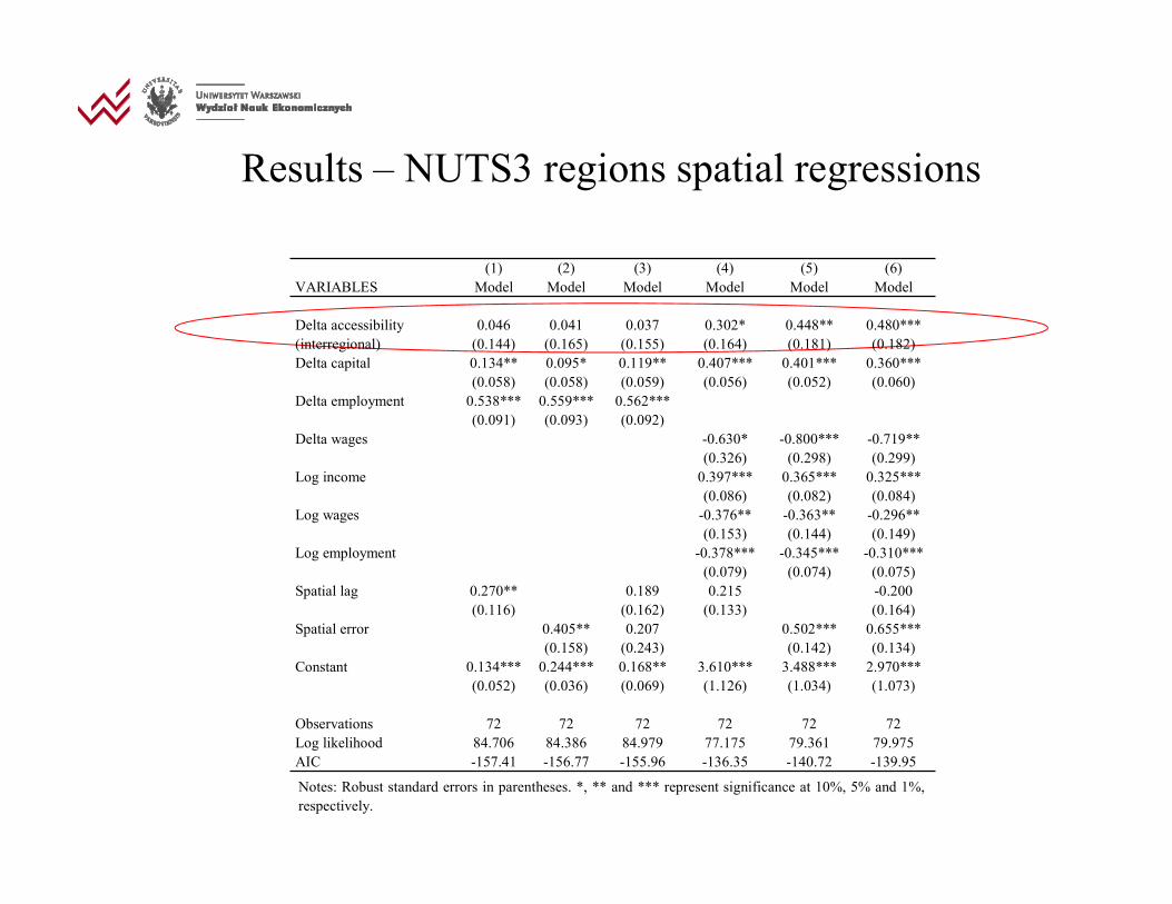
Results – NUTS3 regions spatial regressions

Notes: Robust standard errors in parentheses. *, ** and *** represent significance at 10%, 5% and 1%,respectively.

(1) (2) (3) (4) (5) (6)VARIABLES Model Model Model Model Model Model

Delta accessibility 0.046 0.041 0.037 0.302* 0.448** 0.480***(interregional) (0.144) (0.165) (0.155) (0.164) (0.181) (0.182)Delta capital 0.134** 0.095* 0.119** 0.407*** 0.401*** 0.360***

(0.058) (0.058) (0.059) (0.056) (0.052) (0.060)Delta employment 0.538*** 0.559*** 0.562***

(0.091) (0.093) (0.092)Delta wages -0.630* -0.800*** -0.719**

(0.326) (0.298) (0.299)Log income 0.397*** 0.365*** 0.325***

(0.086) (0.082) (0.084)Log wages -0.376** -0.363** -0.296**

(0.153) (0.144) (0.149)Log employment -0.378*** -0.345*** -0.310***

(0.079) (0.074) (0.075)Spatial lag 0.270** 0.189 0.215 -0.200

(0.116) (0.162) (0.133) (0.164)Spatial error 0.405** 0.207 0.502*** 0.655***

(0.158) (0.243) (0.142) (0.134)Constant 0.134*** 0.244*** 0.168** 3.610*** 3.488*** 2.970***

(0.052) (0.036) (0.069) (1.126) (1.034) (1.073)

Observations 72 72 72 72 72 72Log likelihood 84.706 84.386 84.979 77.175 79.361 79.975AIC -157.41 -156.77 -155.96 -136.35 -140.72 -139.95

Results – LAU1 regions

(1) (2) (3) (4) (5) (6)VARIABLES Model Model Model Model Model Model

Delta accessibility -0.068 0.050 -0.101 0.103 -0.177 0.038(0.106) (0.314) (0.112) (0.114) (0.387) (0.127)

Delta capital 0.128*** 0.046 0.122*** 0.199*** 0.372*** 0.157***(0.026) (0.102) (0.028) (0.037) (0.078) (0.037)

Delta employment 0.173*** 0.216** 0.161***(0.042) (0.090) (0.046)

Delta wages -0.300* -0.126 -0.255(0.177) (0.413) (0.202)

Log income 0.106*** 0.219*** 0.143***(0.019) (0.074) (0.022)

Log wages -0.129* -0.052 -0.115(0.068) (0.100) (0.087)

Log employment -0.115*** -0.210*** -0.129***(0.024) (0.077) (0.029)

Constant 0.292*** 0.260*** 0.309*** 1.453*** 0.822 1.261*(0.024) (0.060) (0.026) (0.507) (0.693) (0.670)

Observations 379 65 314 379 65 314R-squared 0.14 0.07 0.13 0.17 0.35 0.18Adj. R-squared 0.13 0.03 0.12 0.15 0.28 0.16

Notes: Robust standard errors in parentheses. *, ** and *** represent significance at 10%, 5% and 1%,respectively.

Results – LAU1 regions with nonlinearity

(1) (2) (3) (4) (5) (6)VARIABLES Model Model Model Model Model Model

Delta accessibility -0.189 -0.046 -0.255** 0.120 -0.083 0.112(interregional) (0.119) (0.283) (0.127) (0.130) (0.337) (0.148)Delta accessibility square 3.316*** -7.481 3.877*** -0.487 8.512* -1.853(interregional) (1.204) (4.828) (1.263) (1.465) (4.721) (1.605)Delta capital 0.130*** 0.043 0.127*** 0.199*** 0.356*** 0.155***

(0.026) (0.102) (0.027) (0.037) (0.078) (0.037)Delta employment 0.178*** 0.247** 0.171***

(0.042) (0.100) (0.046)Delta wages -0.301* -0.041 -0.257

(0.177) (0.406) (0.201)Log income 0.105*** 0.231*** 0.141***

(0.019) (0.077) (0.022)Log wages -0.128* -0.058 -0.109

(0.068) (0.106) (0.088)Log employment -0.114*** -0.222*** -0.128***

(0.025) (0.079) (0.029)Constant 0.262*** 0.288*** 0.267*** 1.469*** 0.807 1.239*

(0.014) (0.034) (0.016) (0.504) (0.721) (0.671)

Observations 379 65 314 379 65 314R-squared 0.15 0.10 0.15 0.17 0.38 0.18Adj. R-squared 0.15 0.04 0.14 0.15 0.31 0.16

Notes: Robust standard errors in parentheses. *, ** and *** represent significance at 10%, 5% and 1%,respectively.

Accessibility within econometric framework -conclusions

• Applying data for the NUTS3 regions, we find that accessibility improvement seems to be positively correlated with regional employment growth. However, the impact on regional production growth is not statistically significant.

• At the LAU1 level we find that while accessibility improvement is not statistically significant in the case of urban areas it is in fact negatively correlated with output growth in the case of rural areas. The differences between rural and urban areas are though much less clear once we analyze the impact of accessibility improvement on growth of employment.

• The positive relationship between accessibility improvement and regional employment growth seems to prove the importance of transport infrastructure for regional labor markets. The latter is particularly significant while spatial spillovers are taken into account.

Policy recommendations

• In the light of our results, the economic arguments that support the current approach of the EU towards transport infrastructure investment in the TENs should underline the possible benefits related to a more optimal use of land and the gain in individual welfare rather than focusing on long run productivity effects.

• Moreover, alternatives to investments in a high-speed road network should be investigated, such as the development of interregional transport connections.

• Future research should also focus on verifying which particular regions are the winners and which are the losers of accessibility improvement in terms of regional development.

• Bröcker (1998) developed a prototype spatial CGE model with specific transportation technology based on the iceberg approach by Samuelson (1952). Similar methodology was then applied by Kilkenny (1998), Hu (2002) or Bröcker et al. (2001, 2010).

• Different approach, to deal with the transportation within CGE framework, was proposed by Kim et al. (2004). In their case transport system is modelled within the satellite module, with the potential accessibility indicator measuring overall accessibility level. Separate transportation network model is used also in models by Anas and Liu (2007), Vold and Jean-Hansen (2007), Haddad et al. (2015) or Kim et al. (2017).

• Haddad (1999) or Haddad and Hewings (2001) introduce into multiregional CGE specific transport services that provide shipping of goods from producers to consumers. It allows to model the transport costs based on origin-destination pairs, with distance acting as a major factor. This way of modeling transport sector can be also found in MONASH (e.g. Adams et al., 2000) or TERM models (e.g. Horridge, 2011).

Different approaches to model transport infrastructurewithin the CGE framework

• There is an extensive literature on modelling the transport services within the CGE framework. However, there are relatively few studies that focus on analyzing the impact of high-speed road network investment on regional economic development.

• Existing papers usually focus on particular investment projects (e.g., Kim et al., 2004) or particular regions (e.g., Haddad et al., 2011) rather than overall development of the entire road network.

• Moreover, most of the papers consider the possible effects of future investment rather than evaluate the real impact of newly constructed roads. Hence, they apply hypothetical values of accessibility increase or travel cost reduction. In this sense, their results cannot be used to verify the conclusions concerning possible nonlinearity of the impact, that can be drawn from the existing econometric studies.

Previous CGE based analyses

We apply Polish version of recursive TERM model by Horridge (e.g., Horridge, 2011). Here, transport services create transport margins that are included in the final price of a given commodity.

Our model is calibrated for 16 NUTS2 regions and 55 industries, with the 2005 national supply and use tables published by Statistics Poland. During the calibration process, the above tables were supplemented by data on regional industry shares, regional population, occupation shares, distance matrices, etc. The supplementary regional data used both in calibration and baseline scenario simulations came from Statistics Poland and ESRI shapefiles.

The model is solved using the GEMPACK software.

Regional CGE study for Poland

Reduction in travel time between 2005 and 2015 (in %)

Region DŚ KP LB LS ŁD MP MZ OP PK PL PM ŚL ŚK WM WP ZP

DŚ -2.56 -4.47 -7.88 -7.44 -14.94 -1.91 -11.90 -1.60 -7.60 -13.13 -7.05 -2.69 -5.45 -6.76 -4.21 -10.74

KP -4.47 -4.52 -5.27 -6.87 -11.06 -5.57 -4.97 -3.93 -5.80 -1.24 -15.30 -6.39 -7.28 -2.73 -4.03 -2.60

LB -7.88 -5.27 -2.34 -10.94 -4.30 -5.46 -4.87 -4.05 -1.57 -3.08 -7.01 -4.76 -1.44 -3.57 -10.19 -9.09

LS -7.44 -6.87 -10.94 -8.85 -12.27 -4.71 -12.68 -5.82 -8.01 -10.91 -5.39 -5.72 -6.47 -6.06 -5.00 -10.33

ŁD -14.94 -11.06 -4.30 -12.27 -6.02 -1.24 -10.36 -4.73 -2.29 -11.84 -20.07 -2.90 -1.64 -5.38 -11.54 -11.20

MP -1.91 -5.57 -5.46 -4.71 -1.24 -4.80 -5.16 -2.07 -11.34 -6.02 -12.56 -4.51 -2.05 -4.79 -3.74 -7.68

MZ -11.90 -4.97 -4.87 -12.68 -10.36 -5.16 -3.95 -4.89 -2.37 -5.42 -8.86 -6.20 -5.36 -2.91 -12.91 -9.25

OP -1.60 -3.93 -4.05 -5.82 -4.73 -2.07 -4.89 0.00 -8.85 -7.42 -11.73 -2.87 -2.79 -4.78 -3.17 -8.55

PK -7.60 -5.80 -1.57 -8.01 -2.29 -11.34 -2.37 -8.85 -1.92 -2.72 -9.44 -11.46 -1.25 -2.73 -5.81 -8.64

PL -13.13 -1.24 -3.08 -10.91 -11.84 -6.02 -5.42 -7.42 -2.72 -1.08 -4.19 -8.17 -5.38 -1.06 -10.31 -5.26

PM -7.05 -15.30 -7.01 -5.39 -20.07 -12.56 -8.86 -11.73 -9.44 -4.19 -3.36 -14.27 -13.58 -5.56 -8.86 -1.68

ŚL -2.69 -6.39 -4.76 -5.72 -2.90 -4.51 -6.20 -2.87 -11.46 -8.17 -14.27 -8.09 -3.26 -5.76 -4.06 -8.42

ŚK -5.45 -7.28 -1.44 -6.47 -1.64 -2.05 -5.36 -2.79 -1.25 -5.38 -13.58 -3.26 -3.21 -4.84 -5.83 -7.95

WM -6.76 -2.73 -3.57 -6.06 -5.38 -4.79 -2.91 -4.78 -2.73 -1.06 -5.56 -5.76 -4.84 -1.57 -4.53 -2.98

WP -4.21 -4.03 -10.19 -5.00 -11.54 -3.74 -12.91 -3.17 -5.81 -10.31 -8.86 -4.06 -5.83 -4.53 -2.39 -6.23

ZP -10.74 -2.60 -9.09 -10.33 -11.20 -7.68 -9.25 -8.55 -8.64 -5.26 -1.68 -8.42 -7.95 -2.98 -6.23 -1.16

Reduction in transport margin (in million euro)

Region 2005 2006 2007 2008 2009 2010 2011 2012 2013 2014 2015 Cumulative

Dolnośląskie -0.30 -2.78 -0.02 -0.07 -5.11 -0.53 -9.52 -2.82 -0.06 -1.82 -0.01 -23.04

Kujawsko-Pomorskie -2.50 -1.55 -0.03 -0.20 -2.98 -0.01 -10.35 -0.35 -3.33 -1.59 0.00 -22.90

Lubelskie -0.06 -0.23 -0.12 -0.11 -1.04 -0.04 -0.13 -0.41 -3.52 -8.41 0.00 -14.07

Lubuskie -0.27 -3.55 -0.21 -0.90 -0.46 -0.03 -0.37 -0.59 -9.67 -4.34 -0.01 -20.39

Łódzkie -0.02 -1.31 -0.02 -0.06 -0.02 -0.02 -0.18 -18.31 -0.05 -10.66 -0.02 -30.69

Małopolskie -0.39 -0.07 -0.02 -3.80 -11.69 -0.04 -0.26 -12.48 -0.09 -0.26 -0.03 -29.13

Mazowieckie -0.02 -0.17 -1.29 -7.93 -4.76 -5.97 -1.36 -10.78 -4.45 -0.21 -7.73 -44.69

Opolskie -0.24 -0.02 -0.02 -0.07 -0.07 -0.02 -0.14 -0.25 -0.07 -0.36 -0.03 -1.30

Podkarpackie -0.27 -0.12 -0.02 -0.06 -0.13 -0.05 -0.18 -3.36 -5.14 -1.46 -0.10 -10.92

Podlaskie -0.02 -0.07 -0.02 -0.11 -0.23 -0.02 -0.15 -4.37 -0.12 -0.71 -0.22 -6.04

Pomorskie -0.01 -0.02 -10.69 -3.07 -0.02 -0.34 -1.04 -2.45 -0.20 -0.48 0.00 -18.32

Śląskie -22.87 -3.26 -1.37 -0.08 -5.62 -5.99 -29.22 -13.46 -6.59 -11.31 -0.04 -99.80

Świętokrzyskie -0.35 -0.39 -0.02 -0.08 -0.27 -0.05 -7.99 -0.28 -0.41 -0.21 -0.03 -10.07

Warmińsko-Mazurskie -0.03 -0.01 -0.40 -0.55 -0.06 -0.02 -3.49 -4.10 -0.08 -0.15 -0.15 -9.05

Wielkopolskie -0.12 -4.54 -0.02 -0.06 -3.65 -0.02 -0.28 -8.88 -0.04 -8.31 -0.01 -25.92

Zachodniopomorskie -0.18 -0.36 -0.11 -0.13 -1.59 -2.59 -1.97 -0.30 -0.24 -0.70 -0.01 -8.16

Poland -27.66 -18.47 -14.40 -17.27 -37.71 -15.74 -66.63 -83.18 -34.06 -50.98 -8.40 -374.49

High-speed road investment spending in EUR million

RegionTotal investment

(euro million)

Major road infrastructure

investment (euro million)

Share in total

investment (%)

Major road infrastructure

investment per capita (euro)

DŚ 50 970 1 828 3.41 637.3

KP 26 657 1 664 5.98 805.3

LB 22 498 894 3.80 420.3

LS 14 381 1 287 8.54 1277.1

ŁD 40 037 3 979 9.51 1598.0

MP 44 774 927 1.97 278.7

MZ 123 121 3 439 2.65 647.7

OP 12 503 0 0.00 0.0

PK 26 281 2 359 8.57 1131.7

PL 14 241 344 2.31 296.3

PM 36 959 730 1.89 321.4

ŚL 71 379 2 581 3.44 569.0

ŚK 14 409 478 3.15 382.9

WM 17 138 879 4.91 619.7

WP 52 309 1 874 3.38 543.6

ZP 23 723 550 2.20 325.6

Poland 591 380 23 812 4.03 626.5

• For our baseline scenarios, we exogenize key macroeconomic variables such as aggregate employment, aggregate household consumption, aggregate investment or regional real GDP, setting them to values observed in Poland over the 2005-2015 period.

• To accommodate these observations a matching number of technology and taste variables and propensities are endogenized.

• For the counterfactual or policy scenarios these technology/taste variables and propensities are exogenously set to the values computed in the base scenario, while the key macroeconomic variables are endogenous.

• Policy results are presented as percentage differences between counterfactual and base scenarios: differences caused by shock related to the development of high-speed road network (both reduction in transport margin and increase in public spending).

Simulation results

Main macroeconomic results - cumulative differences

Variable 2006 2007 2008 2009 2010 2011 2012 2013 2014 2015

Real investment -0.42 -0.49 -0.57 -1.57 -1.91 -1.80 -1.57 -1.36 -1.33 -1.45

Government spending -0.89 -1.52 -1.94 -4.23 -7.94 -10.63 -11.49 -11.91 -12.14 -12.21

Exports 0.44 0.65 0.78 2.02 3.26 3.78 3.66 3.51 3.50 3.41

Imports -0.18 -0.27 -0.34 -0.82 -1.27 -1.49 -1.51 -1.51 -1.55 -1.59

Real GDP -0.04 -0.08 -0.13 -0.25 -0.44 -0.61 -0.74 -0.82 -0.88 -0.96

Aggregate employment -0.05 -0.08 -0.10 -0.25 -0.41 -0.54 -0.59 -0.62 -0.66 -0.70

Real wages -0.05 -0.08 -0.10 -0.25 -0.41 -0.53 -0.58 -0.61 -0.65 -0.70

Main macroeconomic results at the regional level -cumulative differences

Region Real investment

Government spending

Exports Imports Real GDP

Aggregate employment

Real wages

Dolnośląskie 0.20 -14.16 3.07 -1.00 -0.22 -0.37 -0.36Kujawsko-Pomorskie -10.59 -13.80 3.10 -3.62 -5.41 -2.58 -2.56Lubelskie 0.21 -13.82 4.68 -1.65 -0.36 -0.58 -0.58Lubuskie -11.39 -14.25 3.83 -4.09 -4.28 -2.33 -2.30Łódzkie 0.23 -14.81 3.18 -1.18 -0.32 -0.40 -0.39Małopolskie 0.25 -10.82 3.56 -1.23 -0.23 -0.37 -0.37Mazowieckie 0.15 -11.59 4.29 -1.24 -0.18 -0.42 -0.42Opolskie 0.06 0.00 2.42 -0.47 0.06 -0.13 -0.13Podkarpackie 0.26 -14.60 3.42 -1.04 -0.17 -0.37 -0.36Podlaskie 0.20 -13.06 4.70 -1.57 -0.23 -0.44 -0.44Pomorskie -5.47 -7.53 3.14 -2.47 -3.56 -1.65 -1.64Śląskie 0.25 -13.51 2.83 -1.13 -0.38 -0.36 -0.36Świętokrzyskie 0.29 -13.52 4.11 -1.48 -0.34 -0.50 -0.49Warmińsko-Mazurskie 0.21 -14.63 3.89 -1.37 -0.24 -0.41 -0.41Wielkopolskie -8.13 -11.14 3.01 -3.07 -2.89 -1.61 -1.60Zachodniopomorskie 0.15 -12.81 2.81 -0.79 -0.11 -0.18 -0.18

Main macroeconomic results at the regional level without change in margins

Region Real investment

Government spending

Exports Imports Real GDP

Aggregate employment

Real wages

Dolnośląskie 0.20 -14.15 3.14 -0.93 -0.10 -0.32 -0.32

Kujawsko-Pomorskie -10.59 -13.80 3.28 -3.48 -5.21 -2.51 -2.48

Lubelskie 0.20 -13.82 4.77 -1.57 -0.23 -0.53 -0.53

Lubuskie -11.40 -14.24 4.05 -3.86 -3.93 -2.18 -2.16

Łódzkie 0.23 -14.81 3.31 -1.07 -0.13 -0.33 -0.32

Małopolskie 0.24 -10.82 3.67 -1.11 -0.07 -0.30 -0.30

Mazowieckie 0.15 -11.59 4.78 -1.24 -0.16 -0.46 -0.46

Opolskie 0.05 0.00 2.40 -0.47 0.08 -0.13 -0.12

Podkarpackie 0.26 -14.60 3.47 -1.00 -0.08 -0.34 -0.33

Podlaskie 0.20 -13.06 4.77 -1.51 -0.15 -0.42 -0.41

Pomorskie -5.47 -7.53 3.36 -2.40 -3.45 -1.63 -1.62

Śląskie 0.25 -13.51 3.06 -0.94 -0.06 -0.25 -0.24

Świętokrzyskie 0.28 -13.52 4.21 -1.37 -0.17 -0.44 -0.43

Warmińsko-Mazurskie 0.20 -14.63 3.99 -1.29 -0.13 -0.37 -0.37

Wielkopolskie -8.13 -11.14 3.07 -3.01 -2.77 -1.57 -1.55

Zachodniopomorskie 0.15 -12.81 3.09 -0.78 -0.08 -0.21 -0.20

Accessibility within the CGE framework - conclusions

• The overall impact of high-speed road network development on growth of regional production and employment is relatively small.

• Our results indicate that the most of the impact is due to the change in investment rather than the change in accesibility. However, in the case of certain regions the accessibility improvement seems to have greater impacton GDP than investment (e.g., Dolnośląskie, Łódzkie, Małopolskie, Śląskie).

• There exist significant disparities in the impact between regions with high share of major road infrastructure investment undertaken by private investors and the ones that relied fully on public funding.

• In the case of the former the lack of analyzed investment would lead to relatively significant decrease in real GDP or average employment. In the case of the latter the impact of major road infrastructure investment is almost negligible.