international evidence on fiscal solvency: is fiscal policy

WP/07/56

International Evidence on Fiscal Solvency: Is Fiscal Policy “Responsible”?

Enrique G. Mendoza and Jonathan D. Ostry

© 2007 International Monetary Fund WP/07/56 IMF Working Paper Research Department

International Evidence on Fiscal Solvency: Is Fiscal Policy “Responsible”?

Prepared by Enrique G. Mendoza and Jonathan D. Ostry1

March 2007

Abstract

This Working Paper should not be reported as representing the views of the IMF. The views expressed in this Working Paper are those of the author(s) and do not necessarily represent those of the IMF or IMF policy. Working Papers describe research in progress by the author(s) and are published to elicit comments and to further debate.

This paper looks at fiscal solvency and public debt sustainability in both emerging market and advanced countries. Evidence of fiscal solvency, in the form of a robust positive conditional relationship between public debt and the primary fiscal balance, is established in both groups of countries. Evidence of fiscal solvency is much weaker, however, at high debt levels. These findings suggest that many industrial and emerging market economies, including several where fiscal solvency has been the subject of recent debates, appear to conduct fiscal policy responsibly. Yet our results cannot reject the hypothesis of fiscal insolvency in groups of countries with high debt ratios. JEL Classification Numbers: H6 Keywords: fiscal solvency; fiscal policy; debt sustainability Author’s E-Mail Address: [email protected]; [email protected] 1 We thank Henning Bohn, Giovanni Ganelli, David Hauner, Mohan Kumar, and Marco Terrones for helpful comments and suggestions, and Eric Bang for superb research assistance.

2

Contents Page I. Introduction ........................................................................................................................... 3 II. Model-Based Sustainability Analysis .................................................................................. 5 III. Cross-Country Empirical Analysis of Fiscal Solvency ...................................................... 9

A. Results for Industrial Countries ..................................................................................... 11 B. Results for Emerging Economies................................................................................... 13 C. Results for the Full Sample of Industrial and Emerging Economies ............................. 15 D. Estimates of Long-Run Mean Debt Ratios .................................................................... 16

IV. Conclusion ........................................................................................................................ 18 References................................................................................................................................29 Tables 1. Debt Sustainability Regressions: Industrial Countries .......................................................19 2. Debt Sustainability Regressions: Industrial Countries with High and Low Debt ..............20 3. Debt Sustainability Regressions: Emerging Economies.....................................................21 4. Unconditional Correlations Between the Primary Balance-GDP Ratio and Output Gap...22 5. Debt Sustainability Regressions: Emerging Economies with High and Low Debt............23 6. Debt Sustainability Regressions: Industrial and Emerging Economies..............................24 7. Debt Sustainability Regressions: All Countries With High and Low Debt........................25 8. Long-Run Expected Values of Debt-GDP Ratios ..............................................................26 Figures 1. Public Debt .........................................................................................................................27 2. Actual and Debt-Stabilizing Primary Balances ..................................................................27 3. Conditional and Unconditional Correlations Between Primary Balance and Public Debt............................................................................................................28

3

I. INTRODUCTION

The degree to which the evolution of fiscal policy in a country is consistent with intertemporal solvency—the requirement that public debt not explode in the long run—is a key issue for both industrial and emerging market countries. In the case of the former, the ongoing/looming demographic transition is focusing the attention of policy makers on the need to avoid excessive buildup of public debt, while in the case of middle-income countries with unstable access to global capital markets, the painful economic adjustments associated with debt crises are an important incentive to keep public debt within tolerable bounds. At one level of course, intertemporal solvency is an extremely weak criterion—since it requires only that adjustments to bring policy back on track occur at some point in the future. And given the sovereign’s right to tax and (not) spend, credible changes in these variables can always be assumed to make the problem of insolvency disappear. But markets are unlikely to be impressed by promises that are unsupported by the track record of policy makers, so there is merit in actually examining whether—in a particular country—that track record is consistent with behavior that satisfies an intertemporal budget constraint, or not. Fiscal policy, however, is subject to a whole host of heterogeneous, often transitory, influences that would appear to make disentangling the systematic effect of policy makers’ efforts to adhere to an intertemporal budget constraint very difficult. For example, according to Barro’s (1986) classic tax-smoothing model, temporary increases in government spending (for example due to wars) should be financed by a higher budgetary deficit, while business cycle fluctuations should also be accommodated in a similar way. There may be keen interest therefore in knowing whether movements in budgetary balances that occur alongside these various “shocks” are nevertheless operating in a systematic way to offset the impact of transitory factors, and thereby preventing the debt from getting on to a divergent path. Fortunately, the “Model-based Sustainability” (MBS) approach proposed by Bohn (1998), (2005) provides just such a rigorous framework in which to make judgments about how “responsible” fiscal policy is. The essence of the MBS test is to determine whether increases in public debt elicit increases in the government’s primary fiscal balance (i.e. the balance net of interest payments on the debt), controlling for other determinants of the primary balance. The intuition is that a positive conditional correlation between the debt/GDP ratio and the primary surplus/GDP ratio means that, given the structure of shocks occurring in the background, the fiscal authority reacts to positive changes in the public debt ratio by systematically raising the primary surplus/GDP ratio. Bohn proved that in a regression of the primary surplus against public debt, a measure of the cyclical position of the economy, and the transitory component of government spending, a positive regression coefficient on the debt variable is sufficient to establish that fiscal policy is responsible, i.e., run so as to satisfy the government’s intertemporal budget constraint.

4

Applications of Bohn’s MBS test have focused almost exclusively on running such a test on data for the United States (see Bohn (1998), (2005)).2 The issue, however, is of much broader interest given the greater systemic importance of a number of industrial and emerging market countries than even a few years ago, and the need to view progress in addressing problematic levels of public debt in some countries against the backdrop of the buoyant conditions prevailing in financial markets in recent years and the robust growth of the world economy. Indeed, whether countries are in fact acting in ways that will make debt crises/defaults less likely in the future, or merely riding a wave of benign growth and financing conditions, is a key question that can be addressed using the MBS framework. A further issue that is central to whether countries are fiscally responsible is the degree to which the responsiveness of fiscal policy to debt changes itself depends on the level of the debt. Does responsiveness diminish, or possibly become perverse, as the debt ratio nears very high levels? At what levels of debt does one detect a change in behavior, perhaps reflecting the limits of political tolerance for fiscal stringency in the face of mounting debt? Does evidence of “tipping points” in fiscal responsibility vary between industrial and emerging market countries? Does such evidence point to heightened default risk in one group of countries but not the other? This paper looks at these issues for a large panel of both industrial and emerging market countries. Drawing on a dataset that generally covers the broad public sector (as opposed to the central government) for 34 emerging market and 21 industrial countries over the period 1990–2005, we explore a number of different specifications of the MBS test. Robustness of the conditional relationship between primary surpluses and debt is established across a broad range of possible specifications that allow for nonlinearities in the relation, transitory effects of government purchases and the business cycle, as well as country fixed effects and country-specific serial autocorrelation of error terms. Thus, our main conclusion is that there is indeed strong empirical evidence of a robust positive conditional relationship between primary surpluses and public debt for both emerging market and advanced economies (as well as in a sample that combines the two). This relationship is encouraging from a policy perspective, since it suggests that, far from being prone to excessive default, fiscal policy in many industrial and emerging market countries on the whole operates in a “responsible” manner.

2 An exception is IMF (2003), which reports results from applying Bohn’s test to a panel of advanced and emerging market countries. However, this application used ad-hoc country exclusion restrictions and did not correct for significant serial autocorrelation in the data. In contrast, our analysis uses a sample that is larger in country and time coverage without exclusions and controls for serial autocorrelation. These adjustments reverse the result in IMF (2003) suggesting that industrial countries with high debt respond with larger increases in the primary balance. In addition, we produce new results showing that the fiscal solvency test fails for high-debt countries in general, and we study the connection between fiscal solvency and the cyclical behavior of fiscal policies (particularly the pattern of procyclical primary balances in industrial countries vis-à-vis acyclical or countercyclical primary balances in emerging economies).

5

Our empirical analysis also suggests that the MBS test is a useful tool for separating countries in which fiscal solvency holds from those where it fails. In particular, we find that the conditional positive relationship between debt and primary balances is much weaker in emerging market countries with debt ratios in excess of 50 percent of GDP. Moreover, we sort the countries in each of our three groups of industrial, emerging market, and combined set of countries into high- and low-debt countries relative to the mean and median of each group, and find that the MBS test always rejects fiscal solvency in the high-debt countries. The remainder of this paper is organized as follows. The next section summarizes the analytical framework behind Bohn’s MBS test. Section III presents the results of our empirical analysis. The final section presents the main conclusions.

II. MODEL-BASED SUSTAINABILITY ANALYSIS

This section reviews the main elements of Bohn’s (2005) model-based sustainability framework for testing fiscal solvency. Many empirical studies of fiscal solvency (or public debt sustainability) are based on what he defines as “ad hoc sustainability:” testing whether the time-series properties of fiscal data are consistent with the hypothesis that the expected present value of primary balances, discounted at the interest rate on public debt, equals initial debt.3 In contrast, model-based sustainability requires sustainable fiscal policies to be consistent with the general equilibrium conditions that link the government and the private sector in debt markets. Seen from this perspective, ad hoc sustainability turns out to be a mistaken definition of fiscal solvency because the interest rates on public debt are not the correct discount factor for evaluating the expected present value of primary balances.

The above argument can be illustrated as follows:4 Consider an economy where output (y) and government purchases (g) follow a well-behaved stochastic process such that the state st at date t is given by a pair of realizations st = (yt,gt) and the probability of moving from a state st to a state st+1 is given by a Markov transition density function f(st+1,st). The equilibrium prices of state-contingent assets in this economy are given by the j-periods-ahead pricing kernel Qj(st+j|st) that satisfies a standard optimal asset demand condition:5

( ( ) ( ))

( | ) ( , ).( ( ) ( ))

jt j t j j

j t j t t j tt t

u y s g sQ s s f s s

u y s g sβ + +

+ +

′ −=

′ − (1)

3 Several studies have tested for fiscal solvency following this approach by examining the unit-root and co-integration features of fiscal data. A typical test of ad hoc sustainability would be to determine if there are unit roots in real government revenues, expenditures and debt, and at the same time the deficit inclusive of debt service is stationary. See Bohn (2005) for a good review of the literature on this class of fiscal solvency tests.

4 See Ljungqvist and Sargent (2004) for details.

5 This condition follows from the standard Euler equation that sets the marginal utility cost of giving up a unit of consumption at date t, state st equal to the marginal utility benefit of re-allocating that consumption to date t+1, state st+1 using state-contingent assets.

6

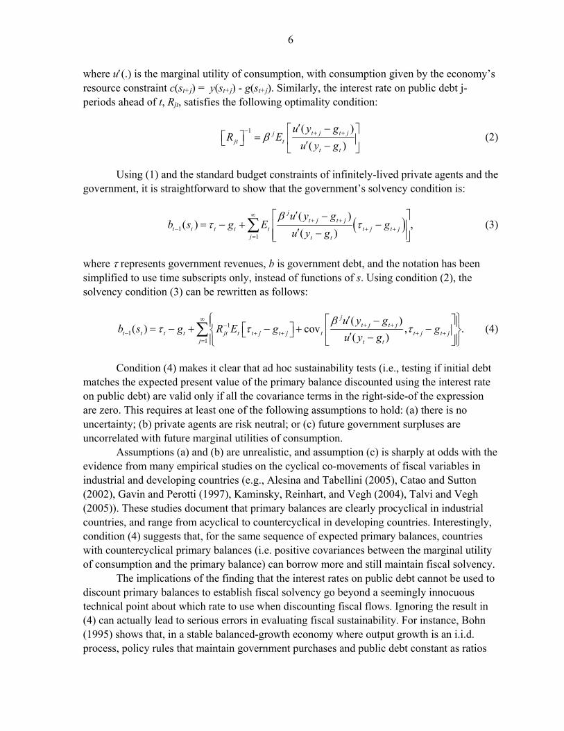
where u′(.) is the marginal utility of consumption, with consumption given by the economy’s resource constraint c(st+j) = y(st+j) - g(st+j). Similarly, the interest rate on public debt j-periods ahead of t, Rjt, satisfies the following optimality condition:

1 ( )

( )t j t jj

jt tt t

u y gR E

u y gβ

− + +′ −⎡ ⎤⎡ ⎤ = ⎢ ⎥⎣ ⎦ ′ −⎣ ⎦

(2)

Using (1) and the standard budget constraints of infinitely-lived private agents and the government, it is straightforward to show that the government’s solvency condition is:

( )11

( )( ) ,

( )

jt j t j

t t t t t t j t jj t t

u y gb s g E g

u y gβ

τ τ∞

+ +− + +

=

′⎡ ⎤−= − + −⎢ ⎥′ −⎢ ⎥⎣ ⎦

∑ (3)

where τ represents government revenues, b is government debt, and the notation has been simplified to use time subscripts only, instead of functions of s. Using condition (2), the solvency condition (3) can be rewritten as follows:

11

1

( )( ) cov , .

( )

jt j t j

t t t t jt t t j t j t t j t jj t t

u y gb s g R E g g

u y gβ

τ τ τ∞

+ +−− + + + +

=

⎧ ⎫′⎡ ⎤−⎪ ⎪⎡ ⎤= − + − + −⎨ ⎬⎢ ⎥⎣ ⎦ ′ −⎪ ⎪⎣ ⎦⎩ ⎭∑ (4)

Condition (4) makes it clear that ad hoc sustainability tests (i.e., testing if initial debt matches the expected present value of the primary balance discounted using the interest rate on public debt) are valid only if all the covariance terms in the right-side-of the expression are zero. This requires at least one of the following assumptions to hold: (a) there is no uncertainty; (b) private agents are risk neutral; or (c) future government surpluses are uncorrelated with future marginal utilities of consumption.

Assumptions (a) and (b) are unrealistic, and assumption (c) is sharply at odds with the evidence from many empirical studies on the cyclical co-movements of fiscal variables in industrial and developing countries (e.g., Alesina and Tabellini (2005), Catao and Sutton (2002), Gavin and Perotti (1997), Kaminsky, Reinhart, and Vegh (2004), Talvi and Vegh (2005)). These studies document that primary balances are clearly procyclical in industrial countries, and range from acyclical to countercyclical in developing countries. Interestingly, condition (4) suggests that, for the same sequence of expected primary balances, countries with countercyclical primary balances (i.e. positive covariances between the marginal utility of consumption and the primary balance) can borrow more and still maintain fiscal solvency.

The implications of the finding that the interest rates on public debt cannot be used to discount primary balances to establish fiscal solvency go beyond a seemingly innocuous technical point about which rate to use when discounting fiscal flows. Ignoring the result in (4) can actually lead to serious errors in evaluating fiscal sustainability. For instance, Bohn (1995) shows that, in a stable balanced-growth economy where output growth is an i.i.d. process, policy rules that maintain government purchases and public debt constant as ratios

7

of GDP violate ad hoc sustainability if mean output growth is greater than or equal to the interest rate on public debt, and yet they satisfy the correct solvency condition (3).

Given the result that ad hoc sustainability tests are not a reliable method to evaluate fiscal solvency, Proposition 1 in Bohn (2005) provides the basis for an alternative test that follows from model-based sustainability: If the primary balance-GDP ratio (pb) is an increasing, linear function of the initial debt-GDP ratio (b), after controlling for other determinants (μ) of the primary balance-output ratio, and if these other determinants measured as GDP ratios are bounded and the present value of output is finite, then the solvency condition (3) holds. Hence, the MBS test consists of estimating the relationship:

1 .t t t tpb bρ μ ε−= + + (5)

where ε is a zero-mean error. The finding that ρ is positive and statistically significant is sufficient to guarantee that condition (3) is satisfied. In most of his tests, Bohn sets the other determinants of the primary balance as 0 1 2t t tg yμ β β β= + +% % , where tg% and ty% are measures of temporary fluctuations in government outlays and GDP respectively. The intuition behind the above result is that, if condition (5) holds, the government budget constraint implies that debt grows between t and t+1 to a level that is (1-ρ) of the level that would imply a Ponzi scheme, so that j periods ahead the debt will be (1-ρ)j the size of a Ponzi scheme’s debt. If 0 < ρ < 1, this means that there is no Ponzi game because

11 1( ) ( | ) (1 ) 0t t j t j j

t t j t j t j tE q s b s s bρ+ + ++ + + + +⎡ ⎤ ≈ − →⎣ ⎦ in the limit as j→∞, where the discount

factor is 11 1 1 2 1

( )( ) ( , ) ( , )... ( , )

( )

jt j t jt t j

t j t j t j t j t j t tt t

u y gq s f s s f s s f s s

u y gβ + ++ +

+ + + + − + − + − +

′ −=

′ −. If ρ >1 then

in fact this expected value diverges to minus infinity as j grows, so the government would be accumulating infinite assets (instead of debt). The MBS test also yields a condition for computing sustainable debt ratios, defined as the mean debt-GDP ratio to which the economy can be expected to converge in the long run. In particular, if the “other” determinants of the primary balance and the growth-adjusted real interest rate on public debt are stationary, with means μ and r respectively, the linear response set in (5) and the government budget constraint yield the following long-run expected value for the public debt-GDP ratio:

[ ] ( )1(1 )cov 1 ,(1 )

t tt

r bE b

r rμ ρ

ρ−− + − +

=+ −

(6)

Notice that, assuming μ ≤0 (as is generally the case in the empirical applications of this setup) and if cov(1+rt ,bt-1) ≥ 0, the mean debt ratio determined in (6) is a negative function of ρ. Thus, everything else constant, a higher ρ indicates reduced average debt in the long run because the government responds with larger primary balances, instead of further borrowing, as past debt rises. Without additional information to establish if these larger

8

primary balances reflect fiscal solvency under optimal fiscal policies, or fiscal solvency under suboptimal policies and/or limited debt market access, we cannot say that higher ρ indicates more fiscal discipline or more sustainable fiscal policies. All we can say is that, as long as ρ is positive and statistically significant, the data indicates that the fiscal solvency condition holds. The situation changes if we can document other features of the fiscal environment that distinguish countries, in addition to estimates of ρ. For example, differences across industrial and emerging economies in average revenue ratios, the volatility of revenues, or the cyclical co-movement of primary balances (see IMF (2003) and Mendoza and Oviedo (2006)) can be useful for evaluating the implications of different values of ρ.

It is important to note three key features of the MBS test: First, since the pricing kernel in (1) applies to all kinds of financial assets, the test does not require particular assumptions about debt management, or the composition of debt in terms of maturity and/or denomination structures. Second, the linear, time-invariant conditional response of the primary balance to debt in eq. (5) is sufficient but not necessary. A non-linear and/or time varying response can also support fiscal solvency as long as the response is strictly positive above a certain threshold debt-output ratio, or the response is at least positive almost surely. Third, the test does not require knowledge of the specific set of government policies on debt, taxes and expenditures. The MBS test determines whether the outcome of a given set of policies implicit in the past primary balance and debt data is in line with the solvency condition (3), without knowing the specifics of those policies.

There are also two important caveats. One is that the equilibrium asset pricing kernel in eq. (1) assumes that there are complete markets of state-contingent claims. Alternatively, one could assume an incomplete-markets economy where the possible realizations of shocks are known but there are not sufficient state-contingent claims to fully hedge against them. In this case, the equilibrium pricing kernel and debt dynamics consistent with fiscal solvency are more difficult to analyze because of precautionary saving behavior (see, for example, Aiyagari and others (2002) and Mendoza and Oviedo (2006)). Still, the results of the MBS tests for emerging economies documented in Section III produce long-run mean debt ratios that are in line with those obtained by Mendoza and Oviedo. This is reasonable because the linear rule specified in (5) yields a well-defined long-run distribution of debt centered around a well-defined mean (see eq. (6) below), and this can be consistent either with the complete-markets solvency condition or with the tighter debt limits imposed by precautionary savings under incomplete markets. Intuitively, the linear response in eq. (5) turns out to be too strong relative to what is needed to ensure that the complete-markets solvency condition (3) holds with equality: A government with positive ρ remains solvent, but it could afford higher indebtedness if markets were complete.

The above intuition does not apply, however, to a “more severe” form of market-incompleteness due to large and fully unanticipated shocks—for example, an unexpected shutdown of credit markets or a surprisingly large negative shock to the primary balance. In this case the problem is not only that the set of state-contingent claims is incomplete, but that there are realizations of shocks that are not in the set that private agents considered to price those claims. In this case, the government can become insolvent (i.e., the expected present

9

value of its primary balances is lower than the value of its debt), and hence results showing that there is a positive and statistically significant conditional response of the primary balance to debt in past data cannot ensure that the response will be enough to maintain fiscal solvency in the future.

The second important caveat of the MBS test relates to how to read results showing that the conditional response of the primary balance to debt is negative or statistically insignificant. Bohn (2005) argues that as long as there is an active market for the debt instruments of a government for which the test fails, and if investors are rational, failures of the test should be seen as evidence that either the intertemporal budget constraint of infinitely-lived agents is not the relevant one (e.g., holders of public debt could have finite lives) or that the failures themselves signal of future policy changes that the market anticipates. The alternative is of course that failures of the test do indicate that the prevailing fiscal policies are unsustainable and that the government is insolvent and headed for default.

III. CROSS-COUNTRY EMPIRICAL ANALYSIS OF FISCAL SOLVENCY

Figure 1 plots the evolution of public debt for industrial and emerging market countries over the period 1992–2005. One feature stands out: industrial countries tend to have higher debt ratios than do emerging market countries. While the debt ratios of both country groups fluctuate widely and these country aggregates can mask important differences in particular country experiences, the fact that industrial countries are able to sustain higher debt ratios than emerging market countries in general remains a key feature of the data.

One possible explanation of this fact can be given by conducting a conventional analysis of debt-stabilizing primary balances, which are defined as the level of the primary balance above which the debt-GDP ratio declines. Figure 2 shows that as of 2005, emerging market countries are about equally divided in terms of those running primary balances that are above or below the debt-stabilizing level, while below-debt-stabilizing primary balances seem to be much less common among the advanced economies. These results suggest that fiscal solvency is weaker in emerging market countries. However, the fact that the primary balance-GDP ratio in a particular year is above or below the debt-stabilizing value does not provide robust evidence of whether fiscal policy is in line with solvency restrictions. This is because the reasoning behind the analysis of debt-stabilizing primary balances suffers from similar problems to those that affect ad hoc fiscal sustainability tests, as reviewed in Section II: both can lead to misleading conclusions as to whether the current primary balance is consistent with fiscal solvency. Hence, in the remainder of this Section we conduct a robust cross-country analysis of fiscal solvency based on the MBS test. Our cross-country application of the MBS test is based on annual data for 22 industrial countries for the period 1970–2005 and 34 developing countries for the period 1990–2005. Within each group, the coverage of country-specific samples varies slightly depending on data availability. The data include: total public debt and primary fiscal balances as shares of GDP at current prices, real GDP, and real government purchases.

Consistent cross-country data on public debt and primary balances are difficult to obtain. For industrial countries, we used data from the OECD’s Analytical Database on gross

10

general government debt and the primary balance of the general government as shares of GDP. For emerging economies, we use debt and primary balance data from an updated dataset produced following the methodology used in the public debt studies in IMF (2003) and Celasun, Debrun and Ostry (2006). These data were put together using information from IMF country desk and fiscal economists for the most comprehensive coverage of the public sector available, which was either the general government or the overall public sector (i.e. the consolidated general government plus public enterprises). These debt data pertain mainly to gross debt and are adjusted to include, where appropriate, debt issued by development banks and debt used to recapitalize domestic banks in the aftermath of banking crises.

Output and government purchases data are from the IMF’s World Economic Outlook database. Since we run these data through the Hodrick-Prescott filter to remove trends, we retrieved the longest time-series available, which for the majority of countries start in 1960. We estimate a cross-country panel version of the MBS test that allows for variation across countries (indexed by i) and over time (indexed by t):

, 0, 1 , 2 , , , ,i t i i t i t i t i tpb g y bβ β β ρ ε= + + + +% % (7)

We allow for country-specific fixed effects, so the intercept can vary across i. In addition, since within-country first-order autocorrelation of the error term is likely given the annual macroeconomic time series used in the regressions, we compare estimates with and without country-specific serial autocorrelation in error terms. In the regressions that assume within country first-order autocorrelation, the error term becomes , , 1 ,i t i i t i tε δ ε η−= + . All the regressions use White cross-section standard errors and covariances to adjust for heteroskedasticity.

The regressions use two alternative sets of measures of temporary fluctuations in government outlays and GDP. One set uses simply the cyclical components of those variables obtained by detrending the data using the Hodrick-Prescott filter with the smoothing parameter set at 100. The resulting detrended series are labeled “output gap” and “government expenditures gap.” The second set follows Bohn (1998) to construct the measures of temporary fluctuations in output and government purchases that enter in the closed-form solution of Barro’s (1986) tax-smoothing model. These measures are defined as GVAR and YVAR for government purchases and output respectively, and the corresponding formulae are:

,T T T T

t t t t t tt tT T

t t t t

g g g y y gGVAR YVARg y y y− −

= = (8)

In these expressions, a superscript T denotes the trend value of the corresponding variable. Note that YVAR is the product of the negative of the percent deviation from trend in output multiplied by the same ratio. Thus, we should expect the sign of β2 obtained in specifications that use YVAR to be the opposite of that produced by specifications that use output gap.

11

Bohn applied this solvency test to long samples of U.S. time series (1916–1995 and 1792–2003 in his (1998) and (2005) articles respectively), and he measured temporary government purchases as the difference between actual and estimated permanent military expenditures. This was done because non-military expenditures are a random walk in long U.S. time series (so they have no transitory component) and because transitory shifts in military spending during large wars are so big that they represent the dominant force driving temporary government spending. Since these two features of the long samples of U.S. data are difficult to establish in our cross-country sample for a much shorter and more recent period, we use a standard definition of temporary government spending as the cyclical component of government expenditures detrended with the Hodrick-Prescott filter. We conducted sensitivity analysis by comparing the results obtained in this way with those produced by measuring temporary government spending as excess government spending above thresholds set in units of standard deviations of the cyclical component of government purchases. These thresholds are a proxy that captures more accurately large spikes in government spending due to wars or natural disasters. The results were largely unaffected by this change.

The panel regressions are separated into three groups. One group for industrial countries (IC group), one for emerging economies (EM group) and one for the full sample of industrial and emerging economies.

A. Results for Industrial Countries

Table 1 presents the results of six panel regressions for the IC sample. Column I shows the results of a univariate regression that uses the debt ratio as the only explanatory variable (other than country fixed effects and autocorrelation coefficients). Columns II and III add the output gap in specifications without correcting for serial autocorrelation (Column II) and with serial autocorrelation corrections (Column III). Columns IV and V add the government purchases gap for the same options with and without correcting for country-specific serial autocorrelation. Column VI is the same regression as in Column V but replacing the output and government purchases gaps with YVAR and GVAR respectively Country-specific estimates of the βi and δi coefficients are not listed in Table 1 and the other tables of panel results to keep the tables short. The full set of results are available from the authors. The univariate regression in Column I yields a positive value for ρ that predicts that increases of 100 basis points in the debt-GDP ratio lead to an increase in the primary balance-GDP ratio of 3.8 basis points. This response is statistically significant at the 95 percent confidence level. The response is about the same but estimated with a smaller standard error in Column II, which adds the output gap but does not correct for autocorrelation. Using the output gap and correcting for autocorrelation in Column III, the response is stronger, at 4.5 basis points, and significant at the 1 percent confidence level. Adding temporary fluctuations in government purchases weakens the response to around 2 basis point in Columns IV-VI. The response is still statistically significant, albeit at the 90 percent confidence level. Columns V and VI show that the shift between the two measures

12

of temporary movements in output and government spending has no effect on the estimated value of ρ or its standard error, and hence does not affect the solvency test. Overall, the IC results are in line with the findings obtained by Bohn (1998) using U.S. data for the period 1916–1995. His estimates of ρ range from 0.028 to 0.054 in the full sample and five subsample periods. The estimates in Bohn (2005), which used data for the period 1792–2003, are somewhat higher, ranging from 0.028 to 0.147 depending on the subsample period, measures of temporary changes in output and government purchases, and estimation method. Hence, we conclude that the panel results for the IC group show that Bohn’s conclusion that there is substantial evidence in favor of fiscal solvency in the United States extends well to a panel of 22 industrial countries with data for the period 1970–2005. Our results for the IC group are also consistent with Bohn’s findings for the United States in indicating the key role that conditioning the response of the primary balance to debt plays. Figure 3 shows conditional and unconditional scatter plots of the primary balance-GDP ratio against the lagged debt-GDP ratio for the IC, EM and FULL groups separately. The conditional plot for the IC group (based on the regression in Column IV of Table 1) shows clearly a positive relationship that is not visible in the unconditional plot. We also conducted two sets of tests to study whether the response of the primary balance to debt varies at different levels of debt. The first set added non-linear coefficients to the regressions by introducing as explanatory variables splines that test for changes in the response of the primary balance to debt above a threshold level of debt, or terms in the square or the cube of deviations of debt from within-country means. None of the coefficients for these nonlinear variables was found to be statistically significant when we added the variables to the regression models in Columns I-VI of Table 1.6 Thus, these results suggest that, within the IC group, there is no identifiable difference in the conditional response of the primary balance to debt as the debt ratio raises above threshold levels, and no significant quadratic or cubic terms in the primary balance-debt relationship. These findings deviate from the results that Bohn (1998) and (2005) found for the United States, where he identified a stronger and statistically significant response of the primary balance to debt at high debt ratios. We show next, however, that we can identify systematic differences in this response when we separate high-debt countries from low debt countries. The second set of tests split the IC sample into two subgroups, high debt (HDIC) and low debt (LDIC) countries. The LDIC (HDIC) subgroup is defined as the industrial countries in our sample with mean and median debt ratios in their country time series that are less or equal (greater) than the mean and median for the full IC panel (i.e. the mean and median calculated using the data for all 22 industrial countries over the entire sample period).7 The 6 As in Bohn (1998), we used spline variables of the form max(0, )b b− . We tried values of b ranging from 0.45 to 0.90, and none of them was statistically significant.

7 If the mean and median for a particular country give conflicting results (i.e., if one moment is above the full IC group moment and the other below), we let the comparison of the medians determine the country’s designation as high or low debt. This only happened in one of the 22 countries, Sweden.

13

mean and median debt ratios in the IC panel are 59 and 57.8 percent respectively. Hence, an industrial country in the HDIC group has a mean debt ratio above 59 percent and a median debt ratio above 57.8 percent. The HDIC group consists of 9 countries and the remaining 13 countries form the LDIC group. Table 2 shows the results for the low-debt, high-debt split. Column I replicates the results from Column VI of Table 1, which includes country-specific autoregressive terms and uses YVAR and GVAR. Column II shows the results for the same regression but applied to the HDIC group and Column III shows the results for the LDIC group. The estimates of the debt-GDP ratio coefficient in the second row of Columns II and III show that the response of the primary balance to debt in the HDIC group is not statistically different from zero, and the point estimate of ρ is in fact negative. The coefficient is positive and significant at the 90 percent confidence level for the LDIC group, and the estimated ρ (0.022) is very close to the estimate obtained using the data for the full IC group in Column I. Thus, the results of the MBS test applied to the low-debt, high-debt split suggest that fiscal solvency cannot be verified in industrial countries with a history of high debt such that the median debt ratio exceeds 57.8 percent and the mean debt ratio exceeds 59 percent.

B. Results for Emerging Economies

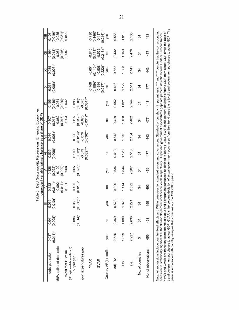
Table 3 presents the results of panel regression models estimated using the data for the EM group. Column I shows results for a univariate, autocorrelation-adjusted regression for which the debt-GDP ratio is the only explanatory variable. Columns II-V show results adding output gap unadjusted and adjusted for autocorrelation (Cols. II-III) and including a spline set at a debt-GDP ratio of 50 percent (Cols. IV-V). Columns VI-IX follow the same ordering adding now gov. expenditures gap. Finally, Columns X-XIII show results replacing output gap and gov. expenditures gap with YVAR and GVAR respectively. The results show that the response of primary balances to debt in the EM group is generally positive and statistically significant in all the regressions. The estimated response without spline adjustments, which ranges from 0.033 in Column X to 0.041 in Column II, varies over a much narrower range than in the case of the IC group, which ranged from 0.02 to 0.045 (see Table 1), and the coefficients are estimated with more precision (they are all significant at the 99 percent confidence level). As in the case of industrial countries, whether we use output gap and government expenditures gap or YVAR and GVAR makes virtually no difference for the estimates of ρ (compare Columns VI with X and VII with XI). Also, the conditional and unconditional scatter plots for the EM group in Figure 3 show again that the conditional plot (produced with the results from Column II in Table 3) yields a clear positive relationship between primary balances and debt, while the unconditional one does not. Tables 1 and 3 yield two important differences in the results of the solvency tests for the IC and EM groups: (1) The estimate of ρ is higher in the EM group. Comparing Column VII of Table 3 with Column V of Table 1, the response to a 100-basis-points increase in the debt ratio is 2 basis points in the IC group v. 3.6 basis points in the EM group.

14

(2) The absolute values of the coefficients on output gap and gov. expenditures gap in the IC group are significantly higher than in the EM group. An increase of 1 percentage point in output gap increases the primary balance-GDP ratio by nearly 1/3 of a percentage point in the IC group, compared to 0.09 of a percentage point in the EM group. An increase in gov. expenditures gap of 1 percentage point reduces the primary balance in the IC group by 0.21 of a percentage point, compared to a reduction of about 0.08 of a percent in the EM group. These differences reflect the sharp contrast between the countercyclical fiscal policies that industrial countries tend to follow and the procyclical fiscal policies common in emerging economies referred to in Section II. Table 4 confirms this pattern in our data. The table lists the unconditional correlations between the primary balance-GDP ratio and output gap for each country in the IC and EM groups. The median correlation is 0.25 in the IC group v. only 0.03 in the EM group.

The above two features that differentiate the IC and EM groups have important implications. On one hand, as explained earlier, the solvency condition (4) implies that, if asset markets are complete, fiscal solvency is compatible with higher debt ratios for countries with acyclical or countercyclical primary balances (i.e., procyclical fiscal policy) than for countries with procyclical primary balances (i.e., countercyclical fiscal policy). Hence, the pattern of primary balance-output gap correlations shown in Table 4 would suggest that EM countries should make more use of debt markets than they seem to make. On the other hand, the higher value of ρ in the EM group implies that these countries must converge to lower mean debt ratios than countries in the IC group, since the long-run expected value of the debt ratio (eq. (6)) is lower as ρ rises. Thus, the higher ρ in the EM group is not an indicator of “more sustainable” fiscal policies. Instead it indicates that an increase in debt of a given magnitude requires a stronger conditional response of the primary balance than in the IC group. This may in turn reflect frictions in asset markets that are more pervasive for EM countries and the riskier fiscal environment they face—they experience acyclical or countercyclical fluctuations in primary balances but at the same time they have access to a limited set of non-state-contingent debt instruments.

The results that include the 50-percent spline in the debt ratio (Columns IV-V, VIII-IX and XII-XIII in Table 3) show that in the case of the EM group, the response of primary balances to debt weakens considerably when the debt ratio is above 50 percent.8 The reduction results in a net effect (i.e. the sum of the coefficients on the debt-GDP ratio and the 50 percent spline) that ranges from 0.023 to 0.029, which is still positive and statistically significant. Thus, even though the response of primary balances to debt falls sharply at high debt ratios, the net response is still positive and significant, and hence the spline does not provide evidence against fiscal solvency as debt grows “too high” in EM countries. This test is not conclusive, however, because it does not separate high-debt from low-debt countries within the EM group. 8 The 50-percent spline was chosen by comparing results with splines ranging from 40 to 90 percent. Splines at 60 percent or more were not statistically significant. From splines between 40 and 60 percent, the one set at 50 percent had the lowest standard error.

15

Table 5 presents panel regression results dividing the EM group into subgroups of countries with high debt (HDEM) and low debt (LDEM), splitting the sample again by assigning countries to the LDEM group if both their mean and median debt ratios are less or equal than the mean and median of the full EM group (which are 64.5 and 58.2 percent respectively). Column I reproduces the results from Column XI in Table 3, and Columns II and III show results for the HDEM and LDEM groups respectively. The HDEM group includes 15 countries and the LDEM group has 19 countries.

The results in Columns II and III of Table 5 are in line with the findings derived from splitting the industrial countries group into high- and low-debt groups. The high-debt group shows an estimate of ρ that is not statistically significant, while the low-debt group yields an estimate of ρ equal to 0.041 and significant at the 99 percent confidence level. Thus, countries in the HDEM group do not appear to follow sustainable fiscal policies. Moreover, comparing the results for low-debt groups in Tables 2 and 5, the estimate of ρ for emerging economies is again higher than for industrial countries (0.041 for the LDEM group v. 0.022 for the HDEM group). This is more evidence in favor of the hypothesis that, among countries that seem to maintain fiscal solvency, emerging economies can be expected to support lower debt levels because they respond with larger primary balances to increases in debt ratios of a given magnitude.

C. Results for the Full Sample of Industrial and Emerging Economies

Tables 6 and 7 present results using the full sample of industrial and developing countries in a similar set of regressions as those applied to the EM and IC groups separately. There are tradeoffs in examining the full sample. One advantage is that the combined group includes 56 countries and about 1000 observations, which is a significantly larger sample than for the EM and IC groups separately. The disadvantage, however, is that the results for the full sample can hide important differences in the behavior of fiscal variables and macroeconomic volatility across countries in the two groups, which have been documented already in discussing the previous results. The results for the full sample have similar features to those for the EM group. The range of estimates of ρ in regressions without splines is the same (from 0.035 to 0.041), and using output gap and gov. expenditures gap or YVAR and GVAR makes no difference again. Moreover, conditioning the response of the primary balance to lagged debt, by controlling for fluctuations in output and government purchases, continues to be very important for identifying the positive response required by the MBS test. The conditional plot for the full sample in Figure 3 (based on the regression in Column IV of Table 6) shows a clear positive response, while the unconditional plot does not.

Regarding results with spline variables, there is a range of splines that are statistically significant, and the one with the lowest standard error is the 48-percent spline for which results are reported in Cols. VI and VIII of Table 6. The net response is again statistically significant and a little higher than in the case of the EM group (about 0.03 instead of ranging from 0.022 to 0.029).

16

Table 7 shows results dividing the full sample into high and low debt groups, defining again low debt countries as those with mean and median debt ratios below the mean and median for the full sample (which are 61.6 and 57.8 percent respectively). Column I reproduces Column VII of Table 6 (the results for the full sample) and Columns II and III show results for high- and low-debt countries. The results are similar to those obtained with the EM and IC groups: the estimate of ρ is not statistically significant for the high-debt group while the estimated value of ρ is 0.04 for the low-debt countries (similar to the value obtained for low debt countries in the EM group) and this estimate is significant at the 99 percent confidence level. In general, the results from the combined IC-EM sample shows that the qualitative findings derived from examining the two country groups separately continue to hold. The key quantitative findings about fiscal solvency, however, are essentially the same as those derived by looking at the EM group alone.

D. Estimates of Long-Run Mean Debt Ratios

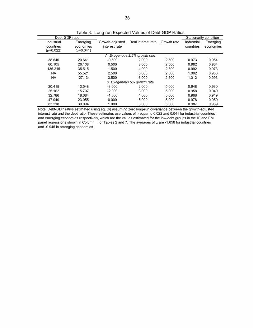
We conclude the empirical analysis by examining the long-run mean debt ratios implied by the results of the MBS tests. As explained earlier, this setup yields an estimate of the sustainable debt ratio defined by the long-run expected value of the debt-output ratio under the assumptions that the determinants of the primary balance, other than debt, and the growth-adjusted real interest rate are stationary (see eq. (6)). For simplicity, we use Bohn’s (2005) approximation to eq. (6), [ ] [ ]/ (1 )E b r rμ ρ≈ − + − , which ignores the long-run covariance between the real interest rate and lagged debt.

Table 8 shows estimates of long-run expected values of the debt-GDP ratio for industrial and emerging economies based on the results of the MBS tests for low-debt countries (LDIC in Column III of Table 2 and LDEM in the same Column of Table 7). This approach uses the most precise estimates of ρ and μ because it sets aside the high-debt countries for which ρ was not statistically significant in both IC and EM groups. The estimates of long-run mean debt ratios also require estimates of r (the difference in the long-run averages of the real interest rate and the per-capita growth rate of real GDP). Panel A of Table 8 shows results assuming a growth rate of 2.5 percent and real interest rates varying from 2 to 6 percent, and Panel B shows results for the same range of real interest rates but using a 5 percent growth rate. The last column of the table shows the product (1+ r )(1-ρ), which must be less than 1 for the debt ratio to be stationary. When this condition is violated, fiscal policy is not sustainable because the debt ratio is not stationary, and so the table shows “NA” for the mean debt ratio. Note that higher ρ reduces (1-ρ) and hence implies that the autocorrelation function of b converges faster to its long-run average.

The results indicate that industrial countries can sustain significantly higher debt ratios (i.e., attain larger mean debt ratios) than emerging economies under common assumptions about growth and interest rates. Assuming the same growth rate for industrial and emerging economies, the differences are larger at lower growth rates, and for a given growth rate they widen as the interest rate rises. At the 5 percent growth rate, the debt ratio of

17

industrial countries exceeds that of emerging economies by 7 percentage points at a 2 percent interest rate, 14 percentage points at a 4 percent interest rate, and 53 percentage points at a 6 percent interest rate. For the 2.5 percent real growth rate, the long-run mean debt ratio in industrial countries exceeds that of emerging economies by 18 percentage points at a 2 percent real interest rate, and at a 4 percent real interest rate the gap widens to 100 percentage points. Note that industrial countries attain higher mean debt ratios because the regressions produce both a lower ρ and a higher absolute value of μ in the LDIC group.

The gap in long-run debt ratios between industrial and developing countries widens even more if we assume that emerging economies grow faster than industrial countries. At a 2 percent interest rate, industrial countries with a long-run growth rate of 2.5 percent converge to a debt-GDP ratio of about 39 percent, while emerging economies growing at 5 percent converge to a 14 percent debt ratio. If emerging economies do reach higher sustained growth rates, however, one would expect that the fundamentals behind the dynamics that determine the values of ρ and μ would also change, and hence these economies could support higher average debt ratios.

It is important to keep in mind that the mean debt ratios in Table 8 represent debt-GDP ratios to which the economy converges on average in the long run given: (a) the information implicit in the conditional feedback response of the primary balance to debt present in the data; (b) the estimated average of the other determinants of the primary balance μ ; (c) the assumptions about average growth and interest rates; and (d) the period government budget constraint: 1(1 )t t t tb r b pb−= + − . Note, in particular, that the mean debt ratios in Table 8 rise as the gap between the interest rate and growth rate widens, up to the point at which the stationarity condition fails.

The result that the mean debt ratio predicted by the MBS setup rises with r seems odd because it is the opposite of the prediction derived from the traditional formula used to calculate long-run debt as the deterministic steady-state debt ratio. This formula states that the steady-state debt ratio is equal to the annuity value of the steady-state primary balance (i.e. b=pb/r), and hence it predicts that the debt ratio should fall as r rises. The two debt ratios have, however, very different meanings. The mean debt ratio of the MBS framework shows the ratio to which the economy converges on average under conditions (a)-(d). If we increase the average growth-adjusted interest rate, keeping all other parameters unchanged and maintaining conditions (a)-(d) (as is the case moving down the rows of Panels A and B in Table 8), the mean debt ratio must rise. This is because the mean debt ratio has implicit a feedback structure driving the stochastic dynamics of the primary balance (given by eq. (5)), and a mapping from these dynamics into sustainable debt via the period government budget constraint. This feedback structure implies that the mean debt ratio rises with r . In contrast, the deterministic steady-state debt ratio simply takes condition (d) and evaluates it at steady-state for arbitrary fixed values of pb and r. Unless appended to a fully-specified dynamic equilibrium model, this steady-state debt ratio cannot tell whether the particular value of pb it uses is a relevant one. Note that, without feedback (i.e. ρ = 0), the equation for the mean debt ratio under the zero covariance assumption collapses to ( ) /( ) [ ]/r E pb rμ− − = , and in this

18

case the mean debt ratio is equal to the deterministic steady-state debt ratio (if we set [ ]pb E pb= and r r= ). This proves that the feedback from debt to primary balances is indeed the reason why the mean debt ratio rises with r .

The mean debt ratios in Table 8 assume exogenous values for growth and interest rates. One straightforward way to endogenize the connection between these two rates is by borrowing from the balanced-growth class of endogenous growth models the basic growth equation ( )1/ ( )rγ σ δ≈ − , where γ is the growth rate, 1/σ is the intertemporal elasticity of

substitution in consumption and δ is the rate of time preference. Under the small open economy assumption, r can be taken from the rest of the world (say set at r=0.06, which is the highest value considered in Table 8). With the standard assumption of σ=2, a discount factor (1/(1+δ))=0.991 would reproduce the 2.5 percent growth rate of Panel A in Table 8 as an “endogenous” growth rate, and would result in the same 127.1 percent mean debt ratio in the second column, last row of Panel A in Table 8. With this endogenous growth rate, however, the results can vary widely for small changes in δ. For example, reducing the discount factor (1/(1+δ))=0.989 yields a decline in the growth rate to 2.39 percent and the fall in the growth-adjusted interest rate results in a higher mean debt ratio of 148.5 percent.

IV. CONCLUSION

This paper examined the issue of fiscal solvency in industrial and emerging market countries. The main finding is that in both groups of countries, the data are consistent with the key requirement of the model-based fiscal sustainability test, namely that the conditional response of primary fiscal balances to changes in government debt be positive. In contrast to the previous literature, we do not find that the responsiveness to debt increases above threshold levels of debt in panel regressions for advanced countries, but it does diminish for emerging market countries. We also find that, if we split each country group into subgroups of high-debt and low-debt countries, the solvency criterion is satisfied for countries with moderate levels of debt, but not for countries with debt levels that surpass the sample mean and median of each group.

The conditional response of primary balances to debt is estimated to be stronger in emerging market than in advanced countries, because the riskier fiscal and financial environment in the former group of countries requires a stronger response to maintain fiscal solvency. This stronger response is therefore not an indicator of more fiscal discipline, as it implies that emerging market countries can sustain lower mean public debt ratios in the long run. We believe the main policy message from our study is that countries should be wary of allowing public debt ratios to rise above the 50–60 percent range: The ability of policy makers to maintain fiscal solvency through higher primary balances in countries with mean and median debt ratios above this range appears to wane.

19

I II III IV V VIdebt-gdp ratio 0.038 0.038 0.045 0.023 0.020 0.020

(0.018)** (0.011)* (0.014)* (0.012)** (0.012)*** (0.012)***output gap 0.269 0.289 0.339 0.309

(0.093)* (0.053)* (0.091)* (0.055)*gov. expenditures gap -0.347 -0.209

(0.081)* (0.041)*YVAR -1.239

(0.211)*GVAR -0.946

(0.186)*Country AR(1) coeffs. yes no yes no yes yes

adj. R2 0.739 0.240 0.760 0.283 0.769 0.767

D.W. 1.595 0.349 1.643 0.367 1.669 1.664

s.e. 1.648 2.825 1.581 2.763 1.558 1.564

No. of countries 22 22 22 22 22 22

No. of observations 514 534 514 524 504 504

Table 1. Debt Sustainability Regressions: Industrial Countries(dependent variable: primary balance as a share of GDP)

Note: All regressions include country fixed effects and White cross-section standard errors and covariances. Standard errors shown in paranthesis. "*," "**" and "***" denote that the corresponding coefficient is statistically significant at the 99, 95 and 90 percent confidence levels respectively. Output and government expenditures gaps are percent deviations from Hodrick-Prescott trends. YVAR and GVAR are transitory components of output and government purchases as defined in Barro (1986). YVAR is the percent deviation of trend GDP from actual GDP times the ratio of trend government purchases to actual GDP. GVAR is the percent deviation of actual government purchases from their trend times the ratio of trend government purchases to actual GDP. The panel is unbalanced with country samples that cover mainly the 1980-2005 period.

20

I II IIIall countries high debt countries low debt countries

c -24.635 -1.058(2.335)* (0.745)

debt-gdp ratio 0.020 -0.013 0.022(0.012)*** (0.026) (0.014)***

YVAR -1.239 -1.414 -1.135(0.211)* (0.356)* (0.237)*

GVAR -0.946 -1.672 -0.533(0.186)* (0.352)* (0.277)**

Country AR(1) coeffs. yes yes yes

adj. R2 0.767 0.794 0.662

D.W. 1.664 1.526 1.813

s.e. 1.564 1.958 1.278

No. of countries 22 9 13

No. of observations 504 196 286

Table 2. Debt Sustainability Regressions: Industrial Countries with High and Low Debt(dependent variable: primary balance as a share of GDP)

Note: All regressions include country fixed effects and White cross-section standard errors and covariances. Standard errors shown in paranthesis. "*," "**" and "***" denote that the corresponding coefficient is statistically significant at the 99, 95 and 90 percent confidence levels respectively. YVAR and GVAR are transitory components of output and government purchases as defined in Barro (1986). YVAR is the percent deviation of trend GDP from actual GDP times the ratio of trend government purchases to actual GDP. GVAR is the percent deviation of actual government purchases from their trend times the ratio of trend government purchases to actual GDP. The panel is unbalanced with country samples that cover mainly the 1980-2005 period. Low debt countries are those with mean and median debt ratios at or below the mean and median of all industrial countries in the sample (which are 59 and 57.8 percent respectively). The low-debt countries are Austria, Australia, Germany, Finland, France, Great Britain, Greece, Norway, New Zealand, Sweden, United States, Iceland, and Luxemburg. High-debt countries are: Canada, Denmark, Spain, Ireland, Italy, Japan, the Netherlands, Portugal,

21

III

IIIIV

VVI

VII

VIII

IXX

XI

XII

XIII

debt

-gdp

ratio

0.03

70.

041

0.03

90.

122

0.12

80.

035

0.03

60.

107

0.10

60.

033

0.03

50.

104

0.10

7(0

.011

)*(0

.008

)*(0

.010

)*(0

.014

)*(0

.022

)*(0

.008

)*(0

.008

)*(0

.013

)*(0

.019

)*(0

.008

)*(0

.008

)*(0

.013

)*(0

.019

)*50

% s

plin

e of

deb

t rat

io-0

.092

-0.1

02-0

.082

-0.0

84-0

.081

-0.0

85(0

.017

)*(0

.029

)*(0

.015

)*(0

.020

)*(0

.016

)*(0

.021

)*W

ald

test

P. v

alue

0.00

10.

068

0.00

30.

032

0.00

70.

046

(H0:

spl

ine=

debt

coe

ffici

ent)

outp

ut g

ap0.

086

0.06

00.

105

0.06

50.

109

0.09

00.

125

0.09

6(0

.014

)*(0

.030

)**

(0.0

13)*

(0.0

23)*

(0.0

12)*

(0.0

19)*

(0.0

12)*

(0.0

16)*

gov.

exp

endi

ture

s ga

p-0

.079

-0.0

76-0

.075

-0.0

73(0

.032

)**

(0.0

36)*

*(0

.031

)**

(0.0

34)*

*YV

AR-0

.769

-0.6

51-0

.845

-0.7

30(0

.109

)*(0

.140

)*(0

.111

)*(0

.146

)*G

VAR

-0.5

44-0

.508

-0.5

29-0

.487

(0.2

17)*

*(0

.222

)**

(0.2

16)*

*(0

.216

)**

Cou

ntry

AR

(1) c

oeffs

.ye

sno

yes

noye

sno

yes

noye

sno

yes

noye

s

adj.

R2

0.52

60.

369

0.52

80.

390

0.53

40.

413

0.54

80.

429

0.55

20.

416

0.55

20.

432

0.55

6

D.W

.1.

829

1.08

01.

828

1.11

41.

844

1.12

61.

813

1.15

81.

821

1.12

21.

808

1.15

31.

813

s.e.

2.22

72.

636

2.22

12.

592

2.20

72.

518

2.15

42.

482

2.14

42.

511

2.14

52.

476

2.13

5

No.

of c

ount

ries

3434

3434

3434

3434

3434

3434

34

No.

of o

bser

vatio

ns45

949

345

949

345

947

744

347

744

347

744

347

744

3

Tabl

e 3.

Deb

t Sus

tain

abilit

y R

egre

ssio

ns: E

mer

ging

Eco

nom

ies

(dep

ende

nt v

aria

ble:

prim

ary

bala

nce

as a

sha

re o

f GD

P)

Not

e: A

ll re

gres

sion

s in

clud

e co

untry

fixe

d ef

fect

s an

d W

hite

cro

ss-s

ectio

n st

anda

rd e

rror

s an

d co

varia

nces

. Sta

ndar

d er

rors

sho

wn

in p

aran

thes

is. "

*" a

nd "*

*" d

enot

e th

at th

e co

rres

pond

ing

coef

ficie

nt is

sta

tistic

ally

sig

nific

ant a

t the

99

and

95 p

erce

nt c

onfid

ence

leve

ls re

spec

tivel

y. O

utpu

t and

gov

ernm

ent e

xpen

ditu

res

gaps

are

per

cent

dev

iatio

ns fr

om H

odric

k-P

resc

ott t

rend

s.

YVA

R a

nd G

VAR

are

tran

sito

ry c

ompo

nent

s of

out

put a

nd g

over

nmen

t pur

chas

es a

s de

fined

in B

arro

(198

6). Y

VAR

is th

e pe

rcen

t dev

iatio

n of

tren

d G

DP

from

act

ual G

DP

tim

es th

e ra

tio o

f tre

nd g

over

nmen

t pur

chas

es to

act

ual G

DP.

GVA

R is

the

perc

ent d

evia

tion

of a

ctua

l gov

ernm

ent p

urch

ases

from

thei

r tre

nd ti

mes

the

ratio

of t

rend

gov

ernm

ent p

urch

ases

to a

ctua

l GD

P. T

he

pane

l is

unba

lanc

ed w

ith c

ount

ry s

ampl

es th

at c

over

mai

nly

the

1990

-200

5 pe

riod.

22

Country Correlation Country CorrelationPortugal -0.542 Pakistan -0.717Greece -0.496 Mexico -0.702Japan -0.244 Egypt -0.661Iseland -0.177 Bulgaria -0.561Norway -0.066 Turkey -0.438Netherlands -0.003 Brazil -0.287Italy 0.068 Croatia -0.254Ireland 0.129 Colombia -0.252New Zealand 0.179 Costa Rica -0.210Belgium 0.223 Uruguay -0.195France 0.244 Morroco -0.187Luxemburg 0.246 Indonesia -0.169United Kingdom 0.293 Venezuela -0.136Austria 0.373 India -0.108Germany 0.374 Argentina -0.099Spain 0.377 Poland -0.054Canada 0.382 Ecuador -0.021United States 0.515 Panama 0.081Australia 0.725 Ukraine 0.088Finland 0.757 South Africa 0.188Sweden 0.822 China 0.209Denmark 0.833 jordan 0.212

Korea 0.219Israel 0.225Chile 0.238Cote d Ivoire 0.286Peru 0.301Hungary 0.302Russia 0.321Nigeria 0.331Philippines 0.349Lebanon 0.493Thailand 0.742Malaysia 0.760

mean 0.228 mean 0.009median 0.245 median 0.030

Industrial countries Emerging economiesTable 4. Unconditional Correlations between the Primary Balance-GDP Ratio and Output Gap

23


c -0.979 0.155 -0.945(0.661) (1.699) (0.320)*

debt-gdp ratio 0.035 0.018 0.041(0.008)* (0.018) (0.006)*

YVAR -0.651 -0.920 -0.726(0.140)* (0.330)* (0.231)*

GVAR -0.508 -0.450 -0.833(0.222)** (0.254) (0.313)*


adj. R2 0.552 0.551 0.543

D.W. 1.808 1.762 1.864

s.e. 2.145 2.480 1.815



Note: All regressions include country fixed effects and White cross-section standard errors and covariances. Standard errors shown in paranthesis. "*" and "**" denote that the corresponding coefficient is statistically significant at the 99 and 95 percent confidence levels respectively. YVAR and GVAR are transitory components of output and government purchases as defined in Barro (1986). The panel is unbalanced with country samples that cover mainly the 1990-2005 period. Low debt countries are those with mean and median debt ratios at or below the mean and median of all emerging countries in the sample (which are 64.5 and 58.2 percent respectively). Low-debt countries are Argentina, Brasil, Mexico, Peru, Turkey, Uruguay, Venezuela, Chile, Korea, Russia, South Africa, Thailand, Colombia, Poland, Ukraine, Costa Rica, China, Croatia and India. High-debt countries are: Malaysia, Hungary, Ecuador, Morocco, Panama, Philippines, Indonesia, Bulgaria, Cote d'Ivoire, Egypt, Israel, Jordan, Lebanon, Nigeria and Pakistan.

Table 5. Debt Sustainability Regressions: Emerging Economies with High and Low Debt(dependent variable: primary balance as a share of GDP)

24

I II III IV V VI VII VIIIdebt-gdp ratio 0.037 0.039 0.041 0.033 0.036 0.071 0.035 0.072

(0.011)* (0.007)* (0.010)* (0.008)* (0.008)* (0.021)* (0.008)* (0.021)*48% spline of debt ratio -0.041 -0.044

(0.020)** (0.021)**Wald test P. value 0.001 0.004

(H0: spline=debt coefficient)output gap 0.126 0.109 0.155 0.138 0.145

(0.028)* (0.028)* (0.026)* (0.019)* (0.018)*gov. expenditures gap -0.099 -0.089 -0.088

(0.027)* (0.030)* (0.030)*YVAR -0.925 -0.957

(0.137)* (0.138)*GVAR -0.570 -0.563

(0.188)* (0.182)*Country AR(1) coeffs. yes no yes no yes yes yes yes

adj. R2 0.649 0.309 0.656 0.340 0.673 0.664 0.669 0.669

D.W. 1.731 0.668 1.740 0.668 1.726 1.721 1.725 1.728

s.e. 1.921 2.737 1.903 2.672 1.854 1.889 1.871 1.874

No. of countries 56 56 56 56 56 56 56 56

No. of observations 988 1042 988 1015 961 920 925 920

Table 6. Debt Sustainability Regressions: Industrial and Emerging Economies(dependent variable: primary balance as a share of GDP)

Note: All regressions include country fixed effects and White cross-section standard errors and covariances. Standard errors shown in paranthesis. "*" and "**" denote that the corresponding coefficient is statistically significant at the 99 and 95 percent confidence levels respectively. Output and government expenditures gaps are percent deviations from Hodrick-Prescott trends. YVAR and GVAR are transitory components of output and government purchases as defined in Barro (1986). YVAR is the percent deviation of trend GDP from actual GDP times the ratio of trend government purchases to actual GDP. GVAR is the percent deviation of actual government purchases from their trend times the ratio of trend government purchases to actual GDP. The panel is unbalanced.

25


c -2.897 -0.689 -1.205(0.968)* (1.385) (0.246)*

debt-gdp ratio 0.035 0.021 0.040(0.008)* (0.015) (0.005)*

YVAR -0.925 -1.232 -0.828(0.137)* (0.242)* (0.174)*

GVAR -0.570 -0.525 -0.771(0.188)* (0.230)** (0.231)*


adj. R2 0.669 0.699 0.593

D.W. 1.725 1.664 1.825

s.e. 1.871 2.111 1.567



Note: All regressions include country fixed effects and White cross-section standard errors and covariances. Standard errors shown in paranthesis. "*" and "**" denote that the corresponding coefficient is statistically significant at the 99 and 95 percent confidence levels respectively. YVAR and GVAR are transitory components of output and government purchases as defined in Barro (1986). The panel is unbalanced. Low debt countries are those with mean and median debt ratios at or below the mean and median of all emerging countries in the sample (which are 61.6 and 57.8 percent respectively). Low-debt countries are Austria, Australia, Finland, France, Great Britain, Norway, New Zealand, Iceland, Luxembourg, Argentina, Brasil, Mexico, Peru, Turkey, Uruguay, Venezuela, Chile, Korea, Russia, South Africa, Thailand, Colombia, Poland, Ukraine, Costa Rica, China, Croatia and India. High-debt countries are: Canada, Germany, Denmark, Spain, Greece, Ireland, Italy, Japan, the Netherlands, Portugal, Sweden, United States, Belgium, Malaysia, Hungary, Ecuador, Morrocco, Panama, Philippines, Indonesia, Bulgaria, Cote d'Ivoire, Egypt, Israel, Jordan, Lebanon, Nigeria and Pakistan.

Table 7. Debt Sustainability Regressions: All Countries with High and Low Debt(dependent variable: primary balance as a share of GDP)

26

Industrial Emerging Growth-adjusted Real interest rate Growth rate Industrial Emergingcountries economies interest rate countries economies(ρ=0.022) (ρ=0.041)

38.640 20.641 -0.500 2.000 2.500 0.973 0.95460.105 26.108 0.500 3.000 2.500 0.982 0.964

135.215 35.515 1.500 4.000 2.500 0.992 0.973NA 55.521 2.500 5.000 2.500 1.002 0.983NA 127.134 3.500 6.000 2.500 1.012 0.993

20.415 13.548 -3.000 2.000 5.000 0.948 0.93025.162 15.707 -2.000 3.000 5.000 0.958 0.94032.786 18.684 -1.000 4.000 5.000 0.968 0.94947.040 23.055 0.000 5.000 5.000 0.978 0.95983.218 30.094 1.000 6.000 5.000 0.987 0.969

Note: Debt-GDP ratios estimated using eq. (6) assuming zero long-run covariance between the growth-adjusted interest rate and the debt ratio. These estimates use values of ρ equal to 0.022 and 0.041 for industrial countriesand emerging economies respectively, which are the values estimated for the low-debt groups in the IC and EMpanel regressions shown in Column III of Tables 2 and 7. The averages of μ are -1.058 for industrial countriesand -0.945 in emerging economies.

B. Exogenous 5% growth rate

Debt-GDP ratio Stationarity conditionTable 8. Long-run Expected Values of Debt-GDP Ratios

A. Exogenous 2.5% growth rate

27

Note: Debt-stabilizing primary balances calculated using the average primary surplus for the 2003–2005 period, the end-2005 debt-GDP ratio, and the average real GDP growth rate for 2000–2005.

Figure 1. Public Debt (in percent of GDP)

55

60

65

70

75

80

1992 1993 1994 1995 1996 1997 1998 1999 2000 2001 2002 2003 2004 2005

Emerging market countries(average)

Industrial countries(average)

Figure 2. Actual and Debt-Stabilizing Primary Balances(in 2005)

-8.0

-6.0

-4.0

-2.0

0.0

2.0

4.0

6.0

8.0

-8.0 -6.0 -4.0 -2.0 0.0 2.0 4.0 6.0 8.0Primary balan ce

Deb

t sta

biliz

ing

Emerging market countries

Industrial countries

29

REFERENCES

Aiyagari, S. Rao. Albert Marcet, Thomas J. Sargent, and Juha Seppälä, 2002, “Optimal Taxation Without State-Contingent Debt,” Journal of Political Economy, Vol. 110 (December), pp. 1220–54.

Alesina, Alberto, and Guido Tabellini, 2005, “Why is Fiscal Policy Often Procyclical,”

IGIER Working Paper No. 297 (Italy: Universita Bocconi). Barro, Robert J., 1979, “On the Determination of Public Debt,” Journal of Political

Economy, Vol. 87, pp. 940–71. ———, 1986, “U.S. Deficits Since World War I,” Scandinavian Journal of Economics,

Vol. 88(1), pp. 195–222. Bohn, Henning, 1995, “The Sustainability of Budget Deficits in a Stochastic Economy,”

Journal of Money, Credit, and Banking, Vol. 27, pp. 257–71. ———, 1998, “The Behavior of U.S. Public Debt and Deficits,” Quarterly Journal of

Economics, Vol. 113(3), pp. 949–63. ———, 2005, “The Sustainability of Fiscal Policy in the United States” (unpublished;

Department of Economics, University of California, Santa Barbara). Catao, Luis A., and Bennett W. Sutton, 2002, “Sovereign Defaults: The Role of Volatility,”

IMF Working Paper 02/149 (Washington: International Monetary Fund). Celasun, Oya, Xavier Debrun, and Jonathan D. Ostry, 2006, “Primary Surplus Behavior and

Risks to Fiscal Sustainability in Emerging Market Countries: A `Fan-Chart' Approach,” IMF Staff Papers, Vol. 53 (December), pp. 401–25.

Gavin, Michael, and Roberto Perotti, 1997, “Fiscal Policy in Latin America,” NBER

Macroeoconomics Annual (MIT Press). International Monetary Fund, 2003, “World Economic Outlook, September 2003: Public

Debt in Emerging Markets,” World Economic and Financial Surveys (Washington: International Monetary Fund).

Ljungqvist, Lars, and Thomas J. Sargent, 2004, Recursive Macroeconomic Theory (MIT

Press).

30

Mendoza, Enrique G., and P. Marcelo Oviedo, 2006, “Fiscal Policy and Macroeconomic Uncertainty in Developing Countries: The Tale of the Tormented Insurer,” NBER Working Paper No. 12586 (Cambridge, Massachusetts: National Bureau of Economic Research).

Talvi, Ernesto, and Carlos Vegh, 2005, “Tax Base Variability and Procyclical Fiscal Policy

in Developing Countries,” Journal of Development Economics, Vol. 78(1), pp. 156–90.

international evidence on fiscal solvency: is fiscal policy

Documents