International Integration and Social Identity∗

Boaz Abramson Moses ShayoDepartment of Economics Department of Economics

Stanford University The Hebrew University of Jerusalemboaza@stanford.edu mshayo@huji.ac.il

October 17, 2021

Abstract

This paper contributes to the literature incorporating social identity into internationaleconomics. We develop a theoretical framework for studying the interplay betweeninternational integration and identity politics, taking into account that both policiesand identities are endogenous. We find that, in general, a union is more fragile whenperipheral member countries have higher status than the Core, as this leads to strongernational identification in equilibrium and a lower willingness to compromise. Low-statuscountries are less likely to secede, even when between-country differences in optimalpolicies are large, and although equilibrium union policies impose significant economichardship. Contrary to the anticipation of some union advocates, mutual solidarity isunlikely to emerge as a result of integration alone.

JEL CODES: F02, F55, E71, Z18.

∗We thank Alberto Alesina, Matthew Gentzkow, Alex Gershkov, Benny Geys, Sergiu Hart, Georg Kirch-steiger, Ilan Kremer, Kostas Makatos, Joram Mayshar, Enrico Spolaore, Guido Tabellini, John Taylor, JeanTirole, Thierry Verdier, Katia Zhuravskaya and many seminar and conference participants for very valuablecomments and suggestions; and Franz Buscha and Jonathan Renshon for sharing their data. Dor Moragprovided excellent research assistance. Financial support from the European Union, ERC Starting Grantproject no. 336659 is gratefully acknowledged.

1 Introduction

The interaction between economic policy and identity politics is increasingly seen as centralfor understanding international economics, from trade policy to currency areas to the Eu-ropean Union (e.g., Grossman and Helpman 2021; Rodrik 2021). Nationalist sentiment, forexample, is often seen as a threat to the European project and is regularly associated with theascent of Eurosceptic political parties (Hobolt and de Vries, 2016; Noury and Roland, 2020).This raises important questions about economic and political integration. Does a commonidentity strengthen a union? Which countries are more likely to join a union and whichare prone to secede when identity and economic considerations interact? Have advocates ofthe European project been overly optimistic in assuming that integration promotes mutualsolidarity, i.e. individuals from one country caring about the wellbeing of individuals fromother member countries? We propose a simple analytical framework to help think aboutthese questions, taking into account what we know about the workings of social identity,and focusing on an equilibrium in which both integration and identities are endogenous. Wehave four main results:

1. Mutual solidarity across countries is unlikely to emerge as a consequence of themjoining an economic union. In fact, unification can push the politically more powerfulcountries in the union (“the Core”) towards a more exclusionary nationalist stance.

2. While economic and political unions can be economically beneficial under some condi-tions, social identity introduces the possibility that low-status periphery countries getcaught in an “identity poverty trap”. For example, European identification can drivesome peripheral European countries to economic concessions in order to stay part ofthe union. These concessions further diminish their national standing relative to Eu-rope as a whole, providing further incentives to seek to identify as European, even asthis undermines their economy.

3. A union with a periphery country that nonetheless enjoys higher status than the Core(e.g. due to its history or international prestige) is inherently fragile. National iden-tification is harder to overcome in high-status countries, which in turn weakens theirwillingness to make policy concessions in order to be part of a union. Disintegration canthus take place despite low fundamental differences in optimal policies across countries.

4. A reduction in the salience of inter-country differences allows a union to survive athigher levels of such differences, and tends to expand the domain where both unificationand a common identity can be sustained.

1

How should we model identity? Research in both economics and psychology documentsthe ways in which individuals associate themselves with groups, and how this affects theirbehavior (for a review see Shayo, 2020). The evidence indicates two broad patterns: (a)caring about the success and wellbeing of one’s group, often manifested in costly preferentialtreatment of this group; and (b) seeking to be similar to other individuals in one’s group.Importantly, such group-related behavior is endogenous: people are more likely to identifywith those groups that are more similar to them and that can make them proud and conferhigher status. Hence, identities not only shape but also respond to economic circumstances.Formally, people gain utility not only from their personal payoffs but also from the success(or “status”) of the group with which they associate themselves. That is, if my group doeswell, my utility increases. However, individuals cannot easily identify with any group towhich they belong, and incur a cognitive cost for identifying with a group that is actuallyquite different from them. Thus, to maximize utility, individuals can engage in two differentstrategies. First, they can seek to increase the status of their group and to reduce theirperceived distance from it. Second, they can change their identities. A German citizen, forexample, may identify as a German but may, to some extent, also identify as a European. Ifthe status of Europe is high relative to that of Germany alone (perhaps due to its history),identifying with Europe can raise that citizen’s utility.

We consider a simple bargaining game between two countries: a Core and a Periphery.Each country has its own optimal policy, reflecting its economic fundamentals, culture, po-litical ideology, etc. Integration entails economic gains to both countries (e.g. from increasedtrade), but means they need to share a common policy. The politically dominant Core sets acommon policy for the union (e.g. monetary, trade, or immigration policy). The Peripherythen chooses whether to join the union or leave and set its own policy. Replicating classicresults, unions in this model are less likely to be sustained in equilibrium when cross-countrydifferences in optimal policies are large. The question is: what policies does the union adopt,and at what point does the union disintegrate? We say that a union is more accommodatingif its policies better suit the needs of the politically weaker Periphery (at some economiccost to the Core). We say a union is more robust if it is sustained under larger differencesin optimal policies between members.

While this model is relevant to many settings in which minority regions may seek seces-sion (Canada, Spain, UK), for concreteness we use the European Union and the eurozoneas the running examples. Thus, one can think of France and Germany as the Core, polit-ically dominant countries within the union, while countries like Denmark, Spain, the UKand Greece are Periphery countries that choose whether or not to be part of the union.Members of each country may identify nationally (i.e. with their country) or they may

2

identify with Europe as a whole. Accordingly, there are four possible identity profiles:(C,P ), (C,E), (E,P ) and (E,E), where the first entry in each pair denotes the identityof members of the Core and the second denotes the identity of members of the Periphery.For example, (C,E) denotes a situation in which members of the Core identify nationallyand Periphery members identify with Europe. It should be stressed that identifying withEurope does not imply disregarding your country and caring only about Europe: it simplymeans placing some weight on the success of, and similarity to, Europe whereas an exclusivenational identity does not.

To begin, consider the subgame perfect Nash equilibrium (SPNE) under a given profileof social identities. Consistent with common views and survey data, a union is more ac-commodating when citizens of the Core identify with Europe. This is partly because theCore then effectively internalizes some of the goals of the Periphery. However, a union isless accommodating when the Periphery identifies with Europe. Leaving the union makes itpsychologically costly for the Periphery to continue identifying as European. Hence, as longas the periphery identifies as European, the Core can preserve the union with smaller con-cessions. Notably, the profile (E,E) in which everyone identifies as European is not alwaysthe most robust. For this to happen, the cost of identifying as European without being inthe union has to be high. Otherwise, the (C,E) profile can be more robust.

Taking social identities as given could, however, be misleading. It is by now well-established that ethnic, national or other social identities are changeable, and respondto the social environment in systematic ways (Chandra 2012; Shayo 2020). This suggeststhat—consciously or unconsciously—individuals choose to identify in a meaningful way withsome of the social categories to which they belong, but not with others; and that economicand political processes can affect this choice. Thus, while in principle we can derive thepolicies under any profile of social identities, it is unclear whether all these identity profilescan in fact be sustained. Recall that people are unlikely to identify with groups that are verydifferent from them or have very low status, when a more similar or higher status alternativeis available. But perceived differences can be endogenous to whether the countries are partof a common union or not; and the status of both the union and of the potential memberstates is also endogenous to integration decisions and to the policies that are in place. Wetherefore focus on the “Social Identity Equilibrium” (SIE), where both identities and policiesare mutually consistent.

Consider the simplest case, in which the countries are ex-ante symmetric in status andsimilarity to the group does not affect identification decisions. In this case, in almost anyequilibrium in which the union is sustained, the Core identifies nationally while the peripheryidentifies with the union (the identity profile is (C,E)). Given any other identity profile, and

3

sufficiently small differences in optimal policies such that the union can be sustained in SPNE,equilibrium policies lead to an (ex-post) status advantage for the politically dominant Core.This means that non-(C,E) profiles would not in fact be sustainable. From this perspective,the expectation that unification by itself would lead to the emergence of a common identityseems misplaced: the very success of a union works to enhance national identification inthe union’s dominant Core countries. This last intuition extends to the more general case.National identification is of course shaped by many forces, but it is a mistake to expectunification per se to act as an automatic antidote. This is our first main finding.

A second important result is that under fairly general conditions, when the Peripheryhas lower status than the Core, unification can be sustained in SIE despite large differencesin optimal policies across countries (Proposition 7). The basic reason is that once agentsare allowed to choose their identity, members of a relatively low-status Periphery will seekto identify with the union. To the extent that it is psychologically easier to identify yourselfas European if you are a member of the EU—or if your currency is the euro—then thisincreases the Periphery’s willingness to make economic concessions in order to be part of theunion. Hence the union can be sustained under larger differences. This happens despite—andto some degree because of—the union’s unaccommodating policies vis-a-vis the Periphery,which accentuate the Periphery’s inferiority.

Our third point is that when the Periphery has equal or higher status than the Core,disintegration can occur despite small differences in optimal policies. Such equilibria arecharacterized by national identification in the Periphery (though not necessarily in the Core),which reinforces the Periphery’s reluctance to make policy concessions.

Fourth, consider policies that alter the salience of inter-regional differences. We findthat when people care less about such differences, the union can be sustained under higherdifferences in optimal policies. Moreover, this (weakly) increases the set of circumstancesin which both unification and an all-European (E,E) identity profile can be sustained inequilibrium.

The paper relates to several strands of literature. The first studies monetary and fiscalunions. In particular, the theory of Optimal Currency Areas starting with Mundell (1961)highlights the difficulty in handling asymmetric shocks with a common monetary policy.The main benefits from joining a currency union are trade increases due to the eliminationof currency conversion costs and greater predictability of prices (Mundell, 1961; Rose andHonohan, 2001), and the ability to overcome inflation by joining a monetary union witha credible anchor country (e.g. Barro and Gordon 1983; Alesina et al. 2002; Aguiar et al.2015; Chari et al. 2020). The theory suggests that countries are more likely to join a currencyunion when they have high price and output comovements with other countries in the union,

4

when they trade more with them, and when they cannot commit to low inflation (Alesina etal. 2002). We propose a simple way to incorporate identity politics into this understandingof monetary unions, thereby improving the political realism of these models.

Second, a growing literature, pioneered by Akerlof and Kranton (2000), examines theimplications of identity in economics (see Chen and Li 2009; Benjamin et al. 2010; Bénabouand Tirole 2011; Chen and Chen 2011; Shayo and Zussman 2011; Lindqvist and Östling2013; Bertrand et al. 2015; Cassan 2015; Holm 2016; Kranton and Sanders 2017; Besley andPersson 2019; Hett et al. 2020). Guriev and Papaioannou (2021) provide a review of theclosely related—and overwhelmingly empirical—literature on populism. The closest to ourpaper are Shayo (2009); Gennaioli and Tabellini (2019); and Grossman and Helpman (2021),who study how social identity shapes policies like redistribution and tariffs. These papersfocus on how the identity profile within a country interacts with that country’s policy. Webuild on these contributions to study how identity can shape interactions between countries.

Third, the literature on the political economy of international integration highlights thetradeoff between the costs of heterogeneity and the gains to unification due, e.g., to mar-ket size, economies of scale, cross-regional externalities, or better monitoring of politicians(Alesina and Spolaore 1997; Bolton and Roland 1997; Casella 2001; Lockwood 2002; Harstad2007; Desmet et al. 2011; Boffa et al. 2015). We develop a model that features such a tradeoffand examine both how the introduction of social identity modifies the political equilibriumand how the political equilibrium affects identification patterns.

Finally, a substantial literature studies public attitudes towards international integration.Many explanations focus on economic factors, but non-economic factors clearly play animportant role (Mayda and Rodrik, 2005). In the European case, the general conclusion ofthis literature is that identity-related concerns are at least as important as economic factorsin explaining support for European integration (Hooghe and Marks 2004; see Hobolt andde Vries 2016 for a review). Data we collected around the Brexit referendum also show that,at least at the individual level, voters’ identity (measured before the referendum) stronglypredicts their voting decisions, controlling for a host of socio-demographic and geographiccharacteristics (Appendix C.1). However, less is known about how such attitudes affectpolicies, and, especially, about the properties of the equilibrium. Does a common identityproduce a more stable union? And what identity patterns can we plausibly expect to emerge?

We proceed as follows. Section 2 presents the model. The following two sections developthe building blocks for our solution concept: the determination of integration policy givensocial identities (Section 3), and the choice of identity (Section 4). Section 5 analyzes theequilibrium in which both policies and identity are endogenous. We conclude in Section 6.

5

2 Model

There are two countries: a “Core” of an economic union, denoted C, and a “Periphery”country P that considers joining or exiting the union. Each country has its own natu-ral endowments, economic and legal institutions, culture, etc. Differences across countriestranslate to different ideal policies. As in Alesina and Spolaore (1997), unification entailseconomic gains to both countries (e.g. from increased trade), but means they need to sharea common policy. We use the Eurozone and the European Union as the running examplesof a union, but the model could also apply to other unions such as the United Kingdomor Spain. Denote by E the super-ordinate category which includes both the Core and thePeriphery (e.g. Europe as a whole). Let λ ∈ (0.5, 1) be the proportion of the population ofE who are members of the Core.1

Members of the Core and the Periphery countries have preferences over a compoundpolicy instrument, which we denote ri for i ∈ {C,P}. This may include macroeconomicpolicy instruments such as the interest rate set by the monetary authority, the exchange rateregime, or various fiscal tools. It could also represent other policies that are jointly set incase of unification, such as regulation and immigration policy. Let r∗i be country i’s idealpolicy, from a standard economic perspective. That is, it is the policy the country’s citizenswould most prefer in the absence of any identity concerns. Thus, differences in r∗i capturefundamental differences in economic conditions and preferences across countries. In SectionC.2 we compute some measures of these differences. Without loss of generality, assume thatr∗C ≥ r∗P . For example, Germany wants higher interest rates than Greece or more regulationthan the UK.

The Core moves first and sets the policy instrument at some level rC = r. The Peripherythen either accepts or rejects this policy.2 If it accepts then rP = rC = r. If it rejects thenit is free to set its own policy. The assumption that the Core is politically more powerful isimportant: it is meant to capture the inherent asymmetry present in most unions. This isessential for understanding some of the fundamental difficulties in the vision of a union thatautomatically engenders solidarity among its members. In Section 3.1 and in Appendix A.5we also discuss the symmetric case where union policy maximizes joint welfare.

Unification entails a per-capita benefit to both countries (or equivalently, breakup en-tails a cost) of size 4. This can come from, e.g., gains from trade, economies of scale in

1We take the social categories themselves (“Europe”, the various nations) as given. We do not modelthe historical-cultural process by which they evolved. Naturally, over the long run these categories maychange. Indeed, our model suggests one avenue for studying this evolution: categories that do not engenderidentification in equilibrium may over time become meaningless and die out.

2Equivalently, all citizens of the union vote over the common policy, and the periphery subsequently holdsits own referendum on whether to stay in the union. Since λ > 0.5 this yields the same results.

6

the production of public goods, or reducing the risk of conflict. The material payoff of arepresentative agent in country i is:

Vi(ri, breakup) = −(ri − r∗i )2 −∆ ∗ breakup (1)

where breakup is an indicator variable taking the value 1 if the two countries do not form aunion and zero otherwise. Abusing notation slightly, we use i to denote both a country anda representative agent of that country.

Notice that we assume policy is “sticky”: once the Core sets the policy, it remains inplace even if the Periphery rejects it. This makes sense if union policies are complex andcannot be changed overnight. E.g., if the UK leaves the EU, it will probably take a longtime for the EU to revise all features of the Single Market as well as other regulations thatwere put in place to accommodate British interests. In Appendix B we provide an analysisof the case where the Core is fully flexible in setting its policy once the Periphery leaves theunion. Conclusions are qualitatively similar.

Social identity. Think of an individual that belongs to several social groups. Anindividual i that identifies with group j cares about the status of group j and takes pride inits success. One consequence is that i’s preferences are to some degree aligned with groupj’s. However, the individual cannot easily identify with a group that is very different fromher, and pays a cognitive cost that increases with her perceived distance from that group.Another way to think about it is that an individual that identifies with group j,seeks to besimilar to group j. This type of behavior is consistent with extensive evidence from a widerange of economic domains (see Shayo (2020) for a review). Let Sj be the status of group jand let dij be the perceived distance between individual i and group j. We then define socialidentification as follows.

Definition 1. Individual i is said to identify with group j if her utility over outcomes isgiven by:

Uij(rC , rP , breakup) = Vi + γSj − βd2ij (2)

where γ > 0, β ≥ 0.

Note that while identity is sometimes studied using survey responses, this formulation ismore fundamental. Identity is not just something people say: it is part of their preferencesand can be revealed by their choices (Atkin et al., 2021). Like tastes, identity resides inthe mind of the individual: people do not need permission from anybody to identify with agiven group, nor is their identification conditional on the identity choices of others. I mayidentify as an American, and take pride in America’s achievements, even if many of theother Americans do not identify as such. This is not to say that other people’s identification

7

decisions do not matter for my identity choices. To the extent that such decisions affectbehavior and policy, they can affect both group status and perceived distances.

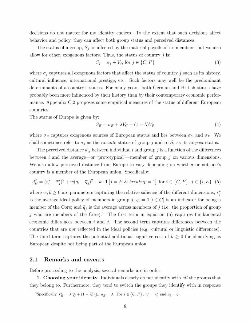
The status of a group, Sj, is affected by the material payoffs of its members, but we alsoallow for other, exogenous factors. Thus, the status of country j is:

Sj = σj + Vj, for j ∈ {C,P} (3)

where σj captures all exogenous factors that affect the status of country j such as its history,cultural influence, international prestige, etc. Such factors may well be the predominantdeterminants of a country’s status. For many years, both German and British status haveprobably been more influenced by their history than by their contemporary economic perfor-mance. Appendix C.2 proposes some empirical measures of the status of different Europeancountries.The status of Europe is given by:

SE = σE + λVC + (1− λ)VP (4)

where σE captures exogenous sources of European status and lies between σC and σP . Weshall sometimes refer to σj as the ex-ante status of group j and to Sj as its ex-post status.

The perceived distance dij between individual i and group j is a function of the differencesbetween i and the average—or “prototypical”—member of group j on various dimensions.We also allow perceived distance from Europe to vary depending on whether or not one’scountry is a member of the European union. Specifically:

d2ij = (r∗i − r∗j)2 + w(qi − qj)2 + k · 1 [j = E & breakup = 1] for i ∈ {C,P} , j ∈ {i, E} (5)

where w, k ≥ 0 are parameters capturing the relative salience of the different dimensions; r∗jis the average ideal policy of members in group j; qi = 1 [i ∈ C] is an indicator for being amember of the Core; and qj is the average across members of j (i.e. the proportion of groupj who are members of the Core).3 The first term in equation (5) captures fundamentaleconomic differences between i and j. The second term captures differences between thecountries that are not reflected in the ideal policies (e.g. cultural or linguistic differences).The third term captures the potential additional cognitive cost of k ≥ 0 for identifying asEuropean despite not being part of the European union.

2.1 Remarks and caveats

Before proceeding to the analysis, several remarks are in order.1. Choosing your identity. Individuals clearly do not identify with all the groups that

they belong to. Furthermore, they tend to switch the groups they identify with in response3Specifically, r∗E = λr∗C + (1− λ)r∗P . qE = λ. For i ∈ {C,P} , r∗i = r∗i and qi = qi.

8

to changes in economic and political conditions (Atkin et al., 2021). Such choices are notnecessarily made consciously and deliberately. Nonetheless, we shall employ an optimizationassumption to capture the major empirical regularities documented in the literature: thatpeople are more likely to identify with those groups that have higher status and that aremore similar to them. This has two important implications. First, not all identity profilescan be sustained. Second, identities respond to economic conditions.

It is important to emphasize that while we often refer to identity as a binary choicebetween a European and a national identity, identifying with Europe may well mean youalso identify with your own country. Formally, when you identify with Europe you put someweight (γ) on European status whereas if you identify exclusively as British you do notplace any weight on European status. Similarly when you identify as European you mayput some weight (β) on your similarity to other Europeans whereas if you only identify asBritish you do not. This interpretation seems consistent with survey data. In our surveyof English voters before the Brexit referendum (see Appendix C.1), roughly 1 percent ofvoters said they saw themselves as European only, whereas about 25% saw themselves asboth British and European. The latter were also far less likely to subsequently vote “leave”than the 70% who saw themselves as British only. In the French Eurobarometer 2014 data,the share of people who see themselves as European only is 1%, whereas 59% see themselvesas both French and European and 40% as French only. France and the UK are not specialin this respect – most Europeans report seeing themselves either as “[nationality] only” oras “[nationality] and European”.

2. Within-country heterogeneity. As pointed out by Bolton and Roland (1997), dif-ferences in income distributions across countries can lead to differences in the ideal policiesof the median voters. Furthermore, within-country heterogeneity is important for under-standing identification patterns (Grossman and Helpman, 2021; Holm, 2016; Lindqvist andÖstling, 2013; Shayo, 2009). Here, we focus on factors such as changes in national status,that move both the elites and the poor in the same direction. Accordingly, one should thinkof the identity profiles we study as reflecting the identity of the decisive players in eachcountry (be they the elites or the median voters), rather than as the complete distributionof identities.

3. Fundamental differences between countries may be endogenous to bothintegration and identification choices, at least in the long run. The direction of these effects,however, is theoretically and empirically ambiguous. On the one hand, integration can leadto specialization (Ricardo 1817; Krugman 1993; Casella 2001). On the other hand, closertrade links may lead to more closely correlated business cycles (Frankel and Rose 1998), andunions may actively seek to homogenize their populations (Weber 1976; Alesina et al. 2019).

9

The evidence for the European case is mixed. Since the 1980’s there appears to have beensome economic convergence across EU countries, at least until the 2008 financial crisis. Butthere is little evidence that EU countries became more similar in fundamental values or inmajor institutional features (Alesina et al. 2017). At this stage we thus take fundamentaldifferences as fixed, but we do analyze changes in the importance that individuals attach tointer-country differences, which arguably can vary even in the short run.

4. Scope. This paper tries to isolate the factors that are essential to understanding thebasic logic of integration and identity. On the political economy side: the trade-off betweengains to unification and costs to heterogeneity, and some asymmetry in power between coreand periphery. On the social identity side: the fact that people care about groups, andthe fundamental factors entering identification decisions (distance and status). This setup,and especially the distinction between core and periphery, may be less relevant to tradeagreements between more symmetric countries. We discuss the symmetric case in Section3.1.4

3 Integration Under Fixed Social Identities

We begin by characterizing the Subgame Perfect Nash Equilibrium (SPNE) under any givenprofile of identities. SPNE is the first building block of our proposed solution concept (SIE,defined in Section 5). It is appropriate for situations where the Core has the political power,i.e., where the Periphery cannot commit to reject offers that are in fact in its interest,thereby forcing its desired policies on the union. Throughout, we impose that in case ofindifference unification occurs. Denote by (IDc, IDP ) the social identity profile in whichCore members identify with group IDc ∈ {C,E} and Periphery members identify withgroup IDP ∈ {P,E} .

Proposition 1. Subgame Perfect Nash Equilibrium (SPNE). For any profile of socialidentities (IDc, IDp), there exist cutoffs R1 = R1(IDc, IDp) and R2 = R2(IDc, IDp) andpolicies rC = rC(IDc, IDp) and rP = rP (IDc, IDp), such that R1 ≤ R2 , rP < rC and:

a. if r∗C − r∗P ≤ R1 then in SPNE unification occurs and rC = rP = rC;b. if R1 < r∗C − r∗P ≤ R2 then in SPNE unification occurs and rC = rP = rP ;c. if r∗C − r∗P > R2 then in SPNE breakup occurs and rC = r∗C , rP = r∗P .

4Even in the European case, the model is naturally a simplification. European integration involves manycountries, many agencies, protracted negotiations and multidimensional policies. Adding specific features of,e.g., the formation of the Eurozone, the Greek debt negotiations, or the Brexit affair, could further enrichthe picture. For example, the Brexit negotiations may have made more salient the differences between theUK and the EU, or may have affected British status. Another possibility is that the breakup revealed toother countries information about 4 (the cost of breakup).

10

Figure 1: General Characterization of SPNE

Proofs are in Appendix A. Figure 1 illustrates. rC reflects the Core’s chosen policy whenthere is no threat of secession. This may or may not be equal to r∗C , depending on the Core’sidentity. When fundamental differences between the countries (r∗C − r∗P ) are small relativeto the cost of dismantling the union, the Periphery country would rather accept rC than setits own ideal policy and suffer the cost of breakup. As a result, the Core sets the policy torC . For larger fundamental differences between the countries (or lower costs of breakup),i.e. when r∗C − r∗P > R1, the Core cannot set the policy to rC while keeping the Peripheryinside the union. However, as long as these differences are smaller than R2, the Core canset its policy at a lower level rP which would keep the Periphery in the union and still bepreferable to breakup. In equilibrium the Periphery country is exactly indifferent betweenstaying in the union and exiting. Finally, when r∗C − r∗P is sufficiently large relative to ∆,i.e. when r∗C − r∗P > R2, the cost required to keep the Periphery in the union exceeds thebenefits to the Core. In this case breakup occurs and policies are set to r∗C and r∗P .

We define two basic properties of unions.

Definition 2. A union is (strictly) more robust if it is sustained under (strictly) largerfundamental differences r∗C − r∗P .

Definition 3. A union is (strictly) more accommodating if the policy implemented is (strictly)closer to r∗P , for any level of fundamental differences such that the union is sustained.

We can now state two preliminary results.

Proposition 2. Robustness. The union is most robust under the (E,E) profile if andonly if βk is sufficiently high. If βk is low, then the union is strictly more robust under the(C,E) profile than under any other identity profile, i.e, R2(C,E) > R2(IDC , IDP ) for all(IDC , IDP ) ∈ {(C,P ), (E,P ), (E,E)}.

Recall that βk is the cognitive cost of maintaining a European identity despite not beinga member of the union. If this cost is sufficiently high, then the all-European identity profile

11

(E,E) is the most robust, since everyone would then be more reluctant to break the union.This is implicitly assumed in many public discussions. Proposition 2, however, shows thatthis is not true in general (see below for more intuition). The next result points out that acommon (E,E) identity does not imply a more accommodating union.

Proposition 3. Accommodationa. The union is more accommodating if Core members identify with Europe rather than

with their nation, for any given Periphery identity,.b. The union is less accommodating if members of the Periphery identify with Europe

rather than with their nation, for any given Core identity.

To see the intuition for these results, we briefly discuss each of the four possible socialidentity profiles. The complete characterization of these cases is given in Lemmas 1-4 inAppendix A. Figure 2 provides an illustration.

Case 1 (C,P ): Both Core and Periphery identify with their own country. Thiscase serves as a convenient benchmark. It essentially replicates the standard analysis ofeconomic integration, in which each country is only interested in its economic payoffs. Atlow fundamental differences, when there is no threat of secession, policy is simply r∗C .Breakup takes place when the material concessions needed to keep the periphery in theunion are larger than the material gains, regardless of how disintegration affects perceiveddistances and European status.

Case 2 (C,E) : Core Identifies with own Country and Periphery with Europe.Comparing this case to Case 1 provides some basic insights into the workings of socialidentity. First, R1(C,E) > R1(C,P ): as long as the Periphery sees itself as European, itprefers r∗C to breakup at relatively higher levels of fundamental differences. Two forces areat work here. First, identifying as European is harder—i.e., generates higher cognitivecosts—when one is not part of the European union. This lowers the value of thePeriphery’s outside option. Second, to the extent that the Periphery sees itself as part ofEurope, its material costs are (somewhat) offset by gains in status stemming from betteroverall European performance. For similar reasons, rP (C,E) > rP (C,P ): even when theCore makes concessions in order to sustain the union, these concessions are smaller thanwhat was needed when the Periphery identified nationally.

Finally, the union can be sustained under larger fundamental differences: R2(C,E) >

R2(C,P ). The difference between R2(C,E) and R2(C,P )—i.e the range of fundamentaldifferences over which the union is sustained under (C,E) but not under (C,P )—dependson several factors: the economic cost of breakup 4, the cognitive cost of breakup k, the size

12

Figure 2: SPNE under Different Social Identity ProfilesNote: This figure does not cover all possible regions of the parameter space. See Lemmas 1-4 in AppendixA for a complete characterization.

of the Core λ, and the weights β and γ that the Periphery places on distance from Europeand on European status. An increase in any one of these tends to make breakup more costlyfor a Periphery that identifies with Europe. This allows the union to be sustained underlarger differences.

Case 3 (E,P ): Core identifies with Europe and Periphery with own Country.Again, it is instructive to compare this case to Case 1. First, rC(E,P ) < rC(C,P ). That is,even when there is no threat of secession, the union is more accommodating since the Corenow internalizes the effects of its policies on European status. Thus, policy is set as someweighted average between the ideal policies of the two countries. In this respect, Europeanidentification implies a measure of solidarity across countries. At some point, however, this

13

policy which takes into account wider European considerations—rC(E,P )—is not sufficientto keep the Periphery in the union and some concessions are needed.5 Since the Peripherycares only about its material payoffs, the policy required to keep it in the union is the sameas in Case 1. Finally, R2(E,P ) ≥ R2(C,P ). Thus, European identity in the Core can alsoforestall breakup.6

Case 4 (E,E): Both Core and Periphery identify with Europe. On the face of it,the case where everyone identifies with the union seems like the most favorable forintegration. Our model suggests a more nuanced view. What is crucial for (E,E) to be themost robust is that the psychological costs of breakup for those who identify as European(βk) are significant. If these psychological costs are low relative to the economic costs 4,then the union is actually less robust when everyone identifies with Europe than when onlythe Periphery does, i.e. R2(E,E) < R2(C,E).

The basic reason is that when fundamental differences between the countries are verylarge, European status would in fact be higher if the Periphery were kept outside the unionand conducted its own policy. If the Core identifies nationally it may seek to sustain theunion even if this depresses European status, as long as this is economically beneficial tothe Core. But if the Core identifies with Europe, then it has to weigh the losses in statusagainst these economic gains, as well as against the psychological gains from keeping thePeriphery in the Union. If the latter are small, breakup can takes place. Regarding policy,as in Case 3, at low levels of fundamental differences, policy is accommodating. Furthermore,the Periphery’s identity means the union is less accommodating in the middle range betweenR1 and R2, which makes it more robust than under either the (C,P ) or (E,P ) profiles.

The role of country size

Is a smaller Periphery more likely to join a union? Our analysis suggests that the answerdepends on social identity. When the Periphery identifies with Europe, a larger relative sizeof the Core means that the Core’s material interests feature more prominently in the Pe-riphery’s considerations, which in turn tends to make breakup more costly for the Periphery.This indeed allows the union to be sustained under larger differences (see Appendix A.1 for

5The reason is that the Core cares about Europe, and not about the Periphery per se. Since Europeanstatus depends on both Core and Periphery material payoffs, rC(E,P ) is not the ideal policy from thePeriphery’s perspective, even if the Core places a very high weight on European status.

6This happens as long as βk > 0. If βk = 0 then R2(E,P ) = R2(C,P ). The reason is that oncefundamental differences are above R1(E,P ), the Periphery’s utility is held constant at the utility obtainedunder breakup. Hence the only factor shifting European status is Core material payoffs. βk = 0 meansthe Core suffers no cognitive cost to breakup, and hence once fundamental differences are such that Corematerial payoffs are higher under breakup than under unification, breakup takes place.

14

details). In other words, the entry of a small nation that identifies as European is likely tobe more robust than the entry of a large nation that identifies this way. However, if thesocial identity profile is (E,P ), the union is less robust when the Core is larger. The higheris λ, the less important is the Periphery in the Core’s identity considerations, which makesthe Core less open to concessions.

3.1 The planner’s solution and the importance of political asym-

metry

In Appendix A.4 we compare the point at which the union disintegrates in SPNE to whata social planner interested in maximizing aggregate material payoffs would do. We findthat national identification in the Periphery tends to produce a less robust union than whatmaterial payoff maximization implies. This echoes the common reaction of economists tothe Brexit vote, which, as we show in Appendix C.1, was associated with strong nationalidentification and weak identification with Europe. A shared identity, however, does notalways enhance overall material payoffs. There exist situations where it is materially optimalto dismantle the union, and yet the union is sustained if the Periphery identifies with Europe.

Finally, in Appendix A.5, we analyze identity effects when there is no asymmetry in sizeor in political power across countries: countries decide whether or not to join the union, andunion policy is set to maximize the joint welfare of its members. We show that in this case,the union is most robust under the (E,E) social identity profile, even if the psychologicalcosts βk are low. This result demonstrates the implications of the Core’s political power.When the Core can make take-it-or-leave-it offers, it may seek to sustain the union at theexpense of the Periphery’s material interests, can do so to a greater extent when the Peripheryidentifies with Europe, and will do so to a greater extent when it identifies nationally. Incontrast, if union policy is constrained to maximize joint welfare, then this channel is shutdown. The union is more robust when the Core identifies with Europe because the welfare-maximizing policy is in this case more accommodating to the Periphery, which providesstronger incentives for the Periphery to join.

4 Choice of Social Identity

We now turn to the determination of social identity. This is the second building block ofour solution concept. We assume that an individual chooses to identify with the group thatyields the highest utility. That is, an individual from country i chooses identity j to solve:

maxj∈{i,E}

Uij(rC , rP , breakup)

15

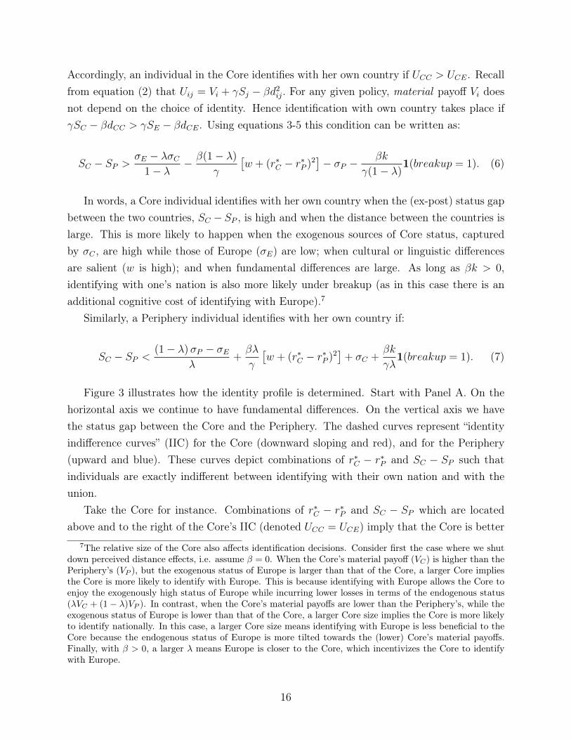
Accordingly, an individual in the Core identifies with her own country if UCC > UCE. Recallfrom equation (2) that Uij = Vi + γSj − βd2ij. For any given policy, material payoff Vi doesnot depend on the choice of identity. Hence identification with own country takes place ifγSC − βdCC > γSE − βdCE. Using equations 3-5 this condition can be written as:

SC − SP >σE − λσC

1− λ− β(1− λ)

γ

[w + (r∗C − r∗P )2

]− σP −

βk

γ(1− λ)1(breakup = 1). (6)

In words, a Core individual identifies with her own country when the (ex-post) status gapbetween the two countries, SC − SP , is high and when the distance between the countries islarge. This is more likely to happen when the exogenous sources of Core status, capturedby σC , are high while those of Europe (σE) are low; when cultural or linguistic differencesare salient (w is high); and when fundamental differences are large. As long as βk > 0,identifying with one’s nation is also more likely under breakup (as in this case there is anadditional cognitive cost of identifying with Europe).7

Similarly, a Periphery individual identifies with her own country if:

SC − SP <(1− λ)σP − σE

λ+βλ

γ

[w + (r∗C − r∗P )2

]+ σC +

βk

γλ1(breakup = 1). (7)

Figure 3 illustrates how the identity profile is determined. Start with Panel A. On thehorizontal axis we continue to have fundamental differences. On the vertical axis we havethe status gap between the Core and the Periphery. The dashed curves represent “identityindifference curves” (IIC) for the Core (downward sloping and red), and for the Periphery(upward and blue). These curves depict combinations of r∗C − r∗P and SC − SP such thatindividuals are exactly indifferent between identifying with their own nation and with theunion.

Take the Core for instance. Combinations of r∗C − r∗P and SC − SP which are locatedabove and to the right of the Core’s IIC (denoted UCC = UCE) imply that the Core is better

7The relative size of the Core also affects identification decisions. Consider first the case where we shutdown perceived distance effects, i.e. assume β = 0. When the Core’s material payoff (VC) is higher than thePeriphery’s (VP ), but the exogenous status of Europe is larger than that of the Core, a larger Core impliesthe Core is more likely to identify with Europe. This is because identifying with Europe allows the Core toenjoy the exogenously high status of Europe while incurring lower losses in terms of the endogenous status(λVC + (1− λ)VP ). In contrast, when the Core’s material payoffs are lower than the Periphery’s, while theexogenous status of Europe is lower than that of the Core, a larger Core size implies the Core is more likelyto identify nationally. In this case, a larger Core size means identifying with Europe is less beneficial to theCore because the endogenous status of Europe is more tilted towards the (lower) Core’s material payoffs.Finally, with β > 0, a larger λ means Europe is closer to the Core, which incentivizes the Core to identifywith Europe.

16

Figure 3: Choice of Social Identity

off identifying nationally (UCC > UCE). Hence, in the region northeast of the Core’s IIC, theidentity profile has to be either (C,P ) or (C,E). However, in the region below and to theleft of the Core’s IIC, the Core identifies with Europe (as both intra-union differences andCore status are relatively low). Hence, the identity profile is either (E,P ) or (E,E). By asimilar logic, the Periphery identifies nationally in the region below and to the right of thePeriphery’s IIC (UPP = UPE), and with Europe above and to the left of it.

In Figure 3.A, ex-ante European status is relatively high.8 Thus, at low differences be-tween the countries, three identity profiles are possible. If the ex-post status gap is sufficientlyhigh, then the only possible identity profile is (C,E). Conversely if SC − SP is sufficientlylow, then the only possible profile is (E,P ). In the intermediate range both the Core andthe Periphery identify with Europe. However, larger differences between the countries makea common European identity harder to sustain. Thus, even when ex-ante European statusis relatively high, an all-European identity profile cannot be sustained if differences betweenthe countries are too large. But large inter-county differences permit the (C,P ) profile.

Figure 3.B illustrates the situation when ex-ante European status is relatively low. Inthis case, the all-European profile (E,E) cannot be sustained, but (C,E) and (E,P ) are stillpossible. Finally note from equations 6 and 7 that breakup shifts both IIC curves inward,making European identification harder to sustain. Importantly, the actual ex-post status gapSC−SP is a function of the policies chosen (Appendix A.6 provides a characterization). Sincethese policies themselves depend on the identity profile, we need to consider the equilibrium.

8That is, above the threshold σ∗E ≡ λσC + (1− λ)σP + βwλ(1−λ)γ + βk

γ 1(breakup = 1).

17

5 Social Identity Equilibrium

We are now in a position to address our main question: what configurations of social identitiesand policies are likely to hold when both are endogenously determined? We employ aconcept of Social Identity Equilibrium (SIE), adapted from Shayo (2009). SIE requiresthat the policies implemented in both countries be a SPNE in the game analyzed in Section3, that is, policies and integration decisions are an equilibrium given the social identityprofile. However, SIE also requires that the social identities themselves be optimal giventhese policies.

Definition 4. A Social Identity Equilibrium (SIE) is a profile of policies (rC , rP , breakup)

and a profile of social identities (IDc, IDp) such that:i. (rC , rP , breakup) is the outcome of a SPNE given (IDc, IDp);ii. IDi ∈ argmax

IDi∈{i,E}Ui,IDi(rC , rP , breakup) for all i ∈ {C,P}.

We begin with the simplest case where there are no ex-ante differences in status and whereperceived distances do not affect identification decisions. Section 5.2 then adds status dif-ferences, and section 5.3 further adds distance effects.

5.1 A simple benchmark

Start by shutting down perceived distance effects, i.e. assume β = 0. Graphically, this meansthat the only thing determining identification decisions is status and hence IICs are flat anddo not depend on unification. Furthermore, suppose there are no ex-ante status differencesbetween the countries. A special case is when status is completely determined by materialpayoffs so that σj = 0 for all j ∈ {C,P,E}.

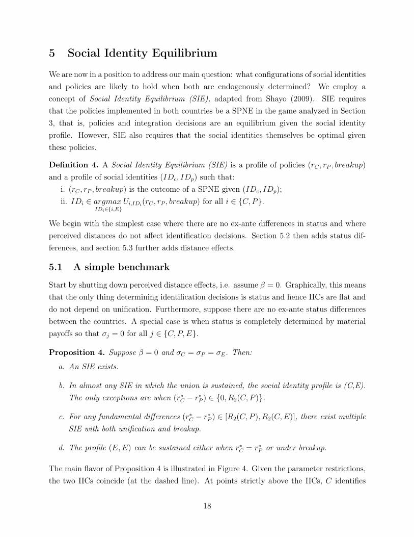
Proposition 4. Suppose β = 0 and σC = σP = σE. Then:

a. An SIE exists.

b. In almost any SIE in which the union is sustained, the social identity profile is (C,E).The only exceptions are when (r∗C − r∗P ) ∈ {0, R2(C,P )}.

c. For any fundamental differences (r∗C − r∗P ) ∈ [R2(C,P ), R2(C,E)], there exist multipleSIE with both unification and breakup.

d. The profile (E,E) can be sustained either when r∗C = r∗P or under breakup.

The main flavor of Proposition 4 is illustrated in Figure 4. Given the parameter restrictions,the two IICs coincide (at the dashed line). At points strictly above the IICs, C identifies

18

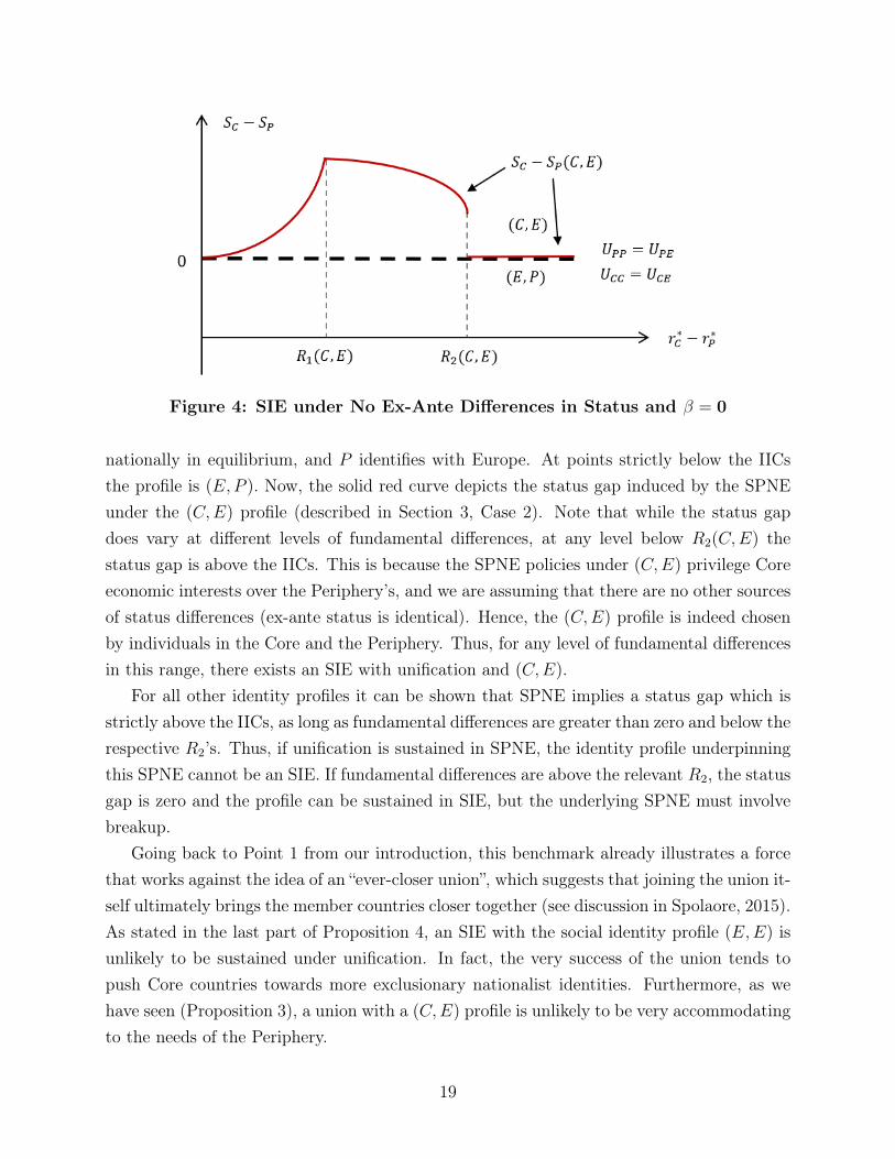
Figure 4: SIE under No Ex-Ante Differences in Status and β = 0

nationally in equilibrium, and P identifies with Europe. At points strictly below the IICsthe profile is (E,P ). Now, the solid red curve depicts the status gap induced by the SPNEunder the (C,E) profile (described in Section 3, Case 2). Note that while the status gapdoes vary at different levels of fundamental differences, at any level below R2(C,E) thestatus gap is above the IICs. This is because the SPNE policies under (C,E) privilege Coreeconomic interests over the Periphery’s, and we are assuming that there are no other sourcesof status differences (ex-ante status is identical). Hence, the (C,E) profile is indeed chosenby individuals in the Core and the Periphery. Thus, for any level of fundamental differencesin this range, there exists an SIE with unification and (C,E).

For all other identity profiles it can be shown that SPNE implies a status gap which isstrictly above the IICs, as long as fundamental differences are greater than zero and below therespective R2’s. Thus, if unification is sustained in SPNE, the identity profile underpinningthis SPNE cannot be an SIE. If fundamental differences are above the relevant R2, the statusgap is zero and the profile can be sustained in SIE, but the underlying SPNE must involvebreakup.

Going back to Point 1 from our introduction, this benchmark already illustrates a forcethat works against the idea of an “ever-closer union”, which suggests that joining the union it-self ultimately brings the member countries closer together (see discussion in Spolaore, 2015).As stated in the last part of Proposition 4, an SIE with the social identity profile (E,E) isunlikely to be sustained under unification. In fact, the very success of the union tends topush Core countries towards more exclusionary nationalist identities. Furthermore, as wehave seen (Proposition 3), a union with a (C,E) profile is unlikely to be very accommodatingto the needs of the Periphery.

19

5.2 Status asymmetry

We now relax the assumption of equal ex-ante status. A rather stark—but arguably com-mon—case is when the Periphery has relatively low ex-ante status:

Proposition 5. Low-Status Periphery. Suppose β = 0 and σC > σE > σP . Then thereexists a unique SIE; the social identity profile is (C,E); and the union is sustained if andonly if (r∗C − r∗P ) ≤ R2(C,E).

As in the benchmark case, if the union is sustained the political power of the Core pushestowards a (C,E) profile. In the present case however, the Core’s political advantage isreinforced by its higher ex-ante status, and the (C,E) profile holds even without unification.

The more important lesson is that the union is more stable in this case. From Proposition4.c we know that under equal ex-ante status there exists a range of fundamental differencesin which both unification and breakup can take place. Proposition 5 however shows thatdifferences in ex-ante status can push the countries towards a unique SIE in which unificationoccurs. This is due to the fact that identity is endogenous. Consider fundamental differenceslarger than R2(C,P ) – the point at which the union disintegrates if the periphery identifiesnationally. Since agents are allowed to choose their identity, the Periphery in this case willchoose to identify with Europe, which in turn permits the union to be sustained under largerdifferences. Recall also that under (C,E) the union is least accommodating (Proposition3). As a result, the status gap (SC − SP ) between the Core and the Periphery widens, andmembers of the Periphery are further motivated to identify with Europe.

This intuition underpins Point 2 from our introduction. As a possible application, con-sider the relationship between the Core Eurozone countries and Greece during the debt crisis.Significant fundamental differences have not led to a “Grexit” from the Eurozone, despitethe grave recession in Greece. Moreover, the Greek government accepted severe austeritymeasures in order to remain in the Eurozone. To be sure, leaving the euro could have enor-mous costs, but unlike Brexit, in the case of southern Europe there is genuine debate amongeconomists regarding the balance of costs and benefits.9 Indeed, from the perspective of themodel, the dismal economic performance of Greece may have even helped sustain a sufficientdegree of European identification among the Greeks which in turn helped keep Greece in theEurozone (see Appendix C.3 for data on support for the euro following the 2008 financialcrisis).

Next, consider the Social Identity Equilibrium when the ex-ante status of the Peripheryis higher than the Core’s. Contrary to the unambiguous nature of Proposition 5, this setting

9With respect to Greece, economists like Joseph Stiglitz argued that “leaving the euro will be painful,but staying in the euro will be more painful” (Stiglitz, J., The Future of Europe, UBS International Centerof Economics in Society, University of Zurich, Basel, January 27, 2014).

20

implies a richer set of possibilities. While the Core continues to enjoy more political power,it no longer has an (ex-ante) status advantage. In the setting of Proposition 5, even ifsome shock drove the Core to temporarily identify with Europe, such an identity would notbe sustainable. However, in the present case political power is counterbalanced by lowerexogenous status and hence European identity in the Core may be sustained. This may thentranslate to equilibria in which the union is sustained and policy is relatively accommodating(e.g. SIE’s with (E,P ) and (E,E) identities). And while (C,E) equilibria may still exist,they are no longer unique.

Proposition 6. High-Status Periphery. Suppose β = 0 and σC < σE < σP . Then:

a. An SIE exists.

b. In any SIE in which breakup occurs, the social identity profile is (E,P ).

c. There exists a subset I∗ ⊆ [R2(C,P ), R2(C,E)] such that if (r∗C − r∗P ) ∈ I∗ both unifi-cation and breakup can occur. However, in any SIE in I∗ in which unification occurs,the Periphery identifies with the union.

Two lessons are worth highlighting. First, the union is more fragile in this case. In contrastto the previous case, in which unification necessarily takes place as long as fundamentaldifferences are below R2(C,E), in this case breakup can occur below this threshold. Thisis illustrated in Figure 5, Panel A. The figure depicts the status gap curve consistent withthe identity profile (E,P ). When this curve lies below both IIC’s, the (E,P ) profile holdsin SIE. However, for fundamental differences above R2(E,P ) the SIE involves breakup. Butwe know from Section 3 that R2(E,P ) < R2(C,E). The conclusion is that unification isnot assured when the Periphery has higher status, even under relatively mild fundamentaldifferences: the status differences can support an identity profile which does not allow forunification in the face of these differences.

Second, consider levels of fundamental differences such that multiple SIE exist wheresome involve breakup and others unification. Proposition 6 says that any SIE in this regionthat involves unification must have the Periphery identify with Europe. This can be seen inFigure 5, Panel B. The figure depicts the status gap functions under three identity profiles.10

The shaded area shows a region of fundamental differences in which multiple equilibria exist,with different identity profiles. Thus, there exists an SIE with breakup and the Peripheryidentifying nationally (the (E,P ) profile – dashed blue curve). But for the same levels of

10The figure is drawn for the case when European status is high, and hence (C,P ) cannot be part of anequilibrium. The intuition for the result is similar in the case when European status is low.

21

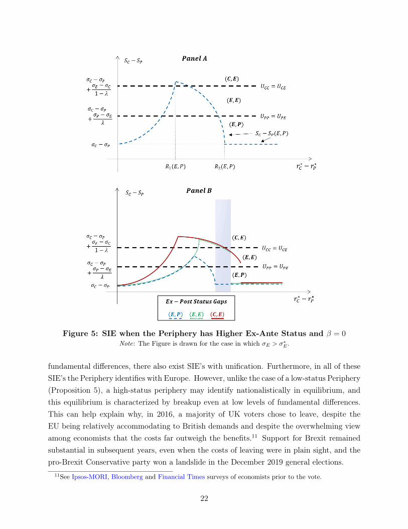
Figure 5: SIE when the Periphery has Higher Ex-Ante Status and β = 0Note: The Figure is drawn for the case in which σE > σ∗E .

fundamental differences, there also exist SIE’s with unification. Furthermore, in all of theseSIE’s the Periphery identifies with Europe. However, unlike the case of a low-status Periphery(Proposition 5), a high-status periphery may identify nationalistically in equilibrium, andthis equilibrium is characterized by breakup even at low levels of fundamental differences.This can help explain why, in 2016, a majority of UK voters chose to leave, despite theEU being relatively accommodating to British demands and despite the overwhelming viewamong economists that the costs far outweigh the benefits.11 Support for Brexit remainedsubstantial in subsequent years, even when the costs of leaving were in plain sight, and thepro-Brexit Conservative party won a landslide in the December 2019 general elections.

11See Ipsos-MORI, Bloomberg and Financial Times surveys of economists prior to the vote.

22

5.3 Distance effects

We now relax the assumption β = 0 to allow identification decisions to respond to perceiveddistances. Let p = (β, k, w, γ,4, λ, σE) be a vector of parameters. Let M(p, σC , σP ) be themaximal level of fundamental differences under which an SIE with unification exists given p

and ex-ante status σC , σP . LetM(p, σC , σP ) be the minimal level of fundamental differencessuch that an SIE with breakup exists for any level of fundamental differences larger thanM(p, σC , σP ), given p, σC , σP .

To begin, consider what happens when σE, the exogenous part of European status, is nottoo high. Specifically:

Condition 1.

σE < min

σC + β(1−λ)2γ

(w + 24+ 2

√42 + β4k

1+γλ+ βk

1+γλ− γk

(1+γλ)(1−λ)

),

λσC + (1− λ)σP + βwλ(1−λ)γ

We can then characterize the SIE as follows.

Proposition 7. Robustness in SIE. Assume Condition 1. Then for any given parametervector p,

a. M (p, σC , σP |σP ≥ σC) ≤M (p, σC , σP |σP < σC), and there exist (p, σC , σP ) such thatthe inequality is strict.

b. M (p, σC , σP |σP ≥ σC) ≤M (p, σC , σP |σP < σC), and there exist (p, σC , σP ) such thatthe inequality is strict.

This result generalizes the patterns discussed in Section 5.2. A union can be sustainedat higher levels of fundamental differences when the Periphery has relatively low status; anddisintegration can occur at lower levels of fundamental differences when the Periphery hasequal or higher status than the Core. The basic reason is that members of a low-statusPeriphery will tend to identify with Europe, which in turn permits the union to be sustainedunder larger differences. This happens despite—and to some degree because of—the unac-commodating policies of the union, which accentuate the Periphery’s status disadvantageand makes European identity more attractive. In contrast, a high-status Periphery is morelikely to adopt a nationalistic identity, which in turn requires a more accommodating policyunder unification. As a result, the union breaks up under smaller differences.

The next two results modify the conclusions from Section 5.2, and provide more insightregarding the identification patterns that emerge under breakup and under unification.

23

Proposition 8. Identification in SIE with Breakup. Assume Condition 1.a. If σP < σC then in any SIE with breakup the Core identifies nationally but the

Periphery may identify with Europe.b. If σP > σC then in any SIE with breakup the Periphery identifies nationally but the

Core may identify with Europe.

Part (a) says that even countries that are not part of the union might still in equilibriumidentify as European, so long as they are low-status. In contrast, high-status countries alwaysidentify nationally under breakup. To see the intuition, consider for a moment what happenswhen σC = σE = σP . Under breakup, each country sets its own policy and there is clearlyno status gain from identifying as European. But identifying with Europe entails a cost interms of perceived distance. Hence, in any SIE with breakup both the Core and the Peripherymust identify nationally. Now, if the Periphery has low ex-ante status, the status gain fromidentifying with Europe may in principle compensate it for the loss in similarity, even at(relatively high) levels of fundamental differences such that breakup occurs. Nonetheless,unlike the special case of β = 0 (Proposition 5), the identity profile under breakup is notnecessarily (C,E), as the Periphery may also identify Nationally.

Conversely, if the Periphery has high ex-ante status, then it identifies nationally in anySIE with breakup. However, the special case of β = 0 (Proposition 6) again needs modifica-tion, as the Core does not necessarily identify with Europe.

Next, consider the identity profile in SIE with unification.

Proposition 9. Identification in SIE with Unification. Assume Condition 1.a. If σP < σC then in any SIE with unification the Core identifies nationally.b. If σP > σC then all four identity profiles can be sustained in some SIE with unification.

Notice that for high status periphery countries, we expect national identification underbreakup (Proposition 8b), but not necessarily under unification. Proposition 9 also confirmsthe point we alluded to earlier: that unification by itself does not guarantee the emergenceof a common identity throughout the union. Most notably, if the Core has high status, thenunification tends to push it towards a more exclusionary identity.12

Finally, consider shocks to β. The thought experiment could be some policy that altersthe salience of inter-country differences.

Proposition 10. Assume Condition 1. Then M(p, σC , σP ) and M(p, σC , σP ) are bothweakly decreasing in β.

12If σC = σP there are more possibilities, depending on β. If β > 0 then like Proposition 9.a, in any SIEwith unification the Core must identify nationally. If β = 0, this is true in almost any SIE with unification(Proposition 4).

24

Thus, a reduction in the salience of inter-country differences—or if people care less aboutthem—would tend to allow the union to be sustained at higher levels of fundamental differ-ences. Moreover, as we show in Appendix A.14, a fall in β would allow new SIE in whichthe Periphery identifies with Europe and unification takes place. However, it is importantto note that when σC ≥ σP the Core identifies nationally in any new SIE which involvesunification. Basically, the gain from identifying with Europe following a decrease in β isoffset by the loss in status.

A more specific question then is what happens to the set of (r∗C − r∗P ) such that thereexists an SIE with both unification and an all-European (E,E) profile. This question hasbeen quite central to the European integration project. We find that in the case of a highstatus periphery (σC ≤ σP ), a fall in β tends to expand this set but this set is unchangedwhen σC > σP (Proposition 15.b in Appendix A.14).

5.4 When the ex-ante status of the union is high

To complete the analysis, consider what happens when we relax Condition 1. We concentratehere on the basic intuition and provide more details in Appendix A.15.

A very high European status makes European identity attractive for a low-status Core.And as long as identifying with Europe implies a cognitive cost of breakup (i.e. βk > 0),then, as discussed in Section 3, this generates an additional incentive for the Core to maintainthe union. Together, these two forces can offset the destabilizing effects of a high-statusperiphery noted in Proposition 7.

Specifically, consider a union with a very high status. Post-WWII USA might be a goodexample. In this case, even if the periphery region has relatively high status (σP > σC), the(E,E) identity profile can be sustained at relatively high fundamental differences. Everyonestill identifies as American. But recall from Proposition 2 that if βk is sufficiently highthen the union is most robust under the (E,E) profile. We can then show that there existparameter values such that (E,E) can be sustained at high fundamental differences when thePeriphery is relatively high-status but not when the Core is. Hence there could be situationswhere M (p, σC , σP |σP ≥ σC) > M (p, σC , σP |σP < σC).

6 Conclusion

Social identity has been widely discussed as an important factor underlying internationaleconomic and political integration. But tracing the implications of identity in this context iscomplicated by the fact that identities can adjust to economic and political conditions. This

25

paper sought to develop a tractable framework that might help us address these issues. Wefocus on the equilibrium in which both policies and identities are endogenously determined.

The analysis offers several lessons. A union with an (ex-ante) high-status peripherycountry tends to be more fragile and may break up at low levels of fundamental differences,compared to a union with a low-status periphery. Importantly—and against the hopesof many supporters of European integration—unification does not necessarily support theemergence of a common identity in equilibrium. Indeed, in the case of relatively high Corestatus, integration can push the Core countries towards a more exclusionary identity. Theanalysis also points to the possibility that low status countries get caught in an identitypoverty trap: low national status generates an incentive to identify as a member of theunion, but such an identification entails a higher cost of breaking up with the union. Thiscan push the periphery country to policy concessions that further erode its status.

To illustrate the applicability of this framework, consider the formation of the eurozone.Countries that joined the euro were not simply countries for whom the loss of monetarypolicy independence was less costly—given similar business cycles as in France and Ger-many—and/or for whom the gains from trade and enhanced credibility were particularlylarge. Rather, they were countries with a combination of high fit in terms of the OptimumCurrency Area (OCA) criteria, and relatively low international status (see Appendix C.2 fora discussion). The eurozone thus included countries that seemed unlikely candidates froman OCA perspective. Countries that stayed out despite their economic suitability to theeuro, tended to be high status countries with relatively high levels of national identification.Similar mechanisms seem to have contributed to avoiding a Grexit despite unaccommodat-ing policies; and to the realization of Brexit, where a high-status country chose to leave theEU despite very accommodating policies. We believe this now calls for empirical analysisto identify and quantify these mechanisms, and to quantitatively assess the role of socialidentity in economic integration more generally.

ReferencesAguiar, Mark, Manuel Amador, Emmanuel Farhi, and Gita Gopinath, “Coordination and crisis in monetary

unions,” The Quarterly Journal of Economics, 2015, 130 (4), 1727–1779.

Akerlof, George A and Rachel E Kranton, “Economics and Identity,” The Quarterly Journal of Economics,2000, 115 (3), 715–753.

Alesina, Alberto and Enrico Spolaore, “On the Number and Size of Nations,” The Quarterly Journal ofEconomics, 1997, 112 (4), 1027–1056.

and Robert J Barro, “Currency unions,” The Quarterly Journal of Economics, 2002, 117 (2), 409–436.

26

, Guido Tabellini, and Francesco Trebbi, “Is Europe an optimal political area?,” Brookings Papers onEconomic Activity, 2017, pp. 169–214.

, Paola Giuliano, and Bryony Reich, “Nation-Building and Education,” Technical Report, NBER WorkingPaper No. 18839 2019.

, Robert J Barro, and Silvana Tenreyro, “Optimal Currency Areas,” NBER Macroeconomics Annual, 2002,17, 301–345.

Atkin, David, Eve Colson-Sihra, and Moses Shayo, “How do we choose our identity? a revealed preferenceapproach using food consumption,” Journal of Political Economy, 2021, 129 (4).

Barro, Robert J and David B Gordon, “Rules, discretion and reputation in a model of monetary policy,”Journal of monetary economics, 1983, 12 (1), 101–121.

Becker, Sascha O, Thiemo Fetzer, and Dennis Novy, “Who voted for Brexit? A comprehensive district-levelanalysis,” Economic Policy, 2017, 32 (92), 601–650.

Bénabou, Roland and Jean Tirole, “Identity, morals, and taboos: Beliefs as assets,” The Quarterly Journalof Economics, 2011, 126 (2), 805–855.

Benjamin, Daniel J, James J Choi, and A Joshua Strickland, “Social Identity and Preferences.,” The AmericanEconomic Review, 2010, 100 (4), 1913–1928.

Bertrand, Marianne, Emir Kamenica, and Jessica Pan, “Gender identity and relative income within house-holds,” The Quarterly Journal of Economics, 2015, 130 (2), 571–614.

Besley, Tim and Torsten Persson, “The Rise of Identity Politics,” Technical Report, Mimeo, LSE 2019.

Boffa, Federico, Amedeo Piolatto, and Giacomo AM Ponzetto, “Political centralization and governmentaccountability,” The Quarterly Journal of Economics, 2015, 131 (1), 381–422.

Bolton, Patrick and Gerard Roland, “The breakup of nations: a political economy analysis,” The QuarterlyJournal of Economics, 1997, 112 (4), 1057–1090.

Casella, Alessandra, “The role of market size in the formation of jurisdictions,” The Review of EconomicStudies, 2001, 68 (1), 83–108.

Cassan, Guilhem, “Identity-based policies and identity manipulation: Evidence from colonial Punjab,” Amer-ican Economic Journal: Economic Policy, 2015, 7 (4), 103–31.

Chandra, Kanchan, Constructivist Theories of Ethnic Politics, Oxford University Press, 2012.

Chari, Varadarajan V, Alessandro Dovis, and Patrick J Kehoe, “Rethinking optimal currency areas,” Journalof Monetary Economics, 2020, 111, 80–94.

Chen, Roy and Yan Chen, “The potential of social identity for equilibrium selection,” American EconomicReview, 2011, 101 (6), 2562–89.

Chen, Yan and Sherry Xin Li, “Group identity and social preferences,” The American Economic Review,2009, 99 (1), 431–457.

Clerc, Laurent, Harris Dellas, and Olivier Loisel, “To be or not to be in monetary union: A synthesis,”Journal of International Economics, 2011, 83 (2), 154–167.

Desmet, Klaus, Michel Le Breton, Ignacio Ortuño-Ortín, and Shlomo Weber, “The stability and breakup ofnations: a quantitative analysis,” Journal of Economic Growth, 2011, 16 (3), 183.

27

Fleming, J Marcus, “On exchange rate unification,” the economic Journal, 1971, 81 (323), 467–488.

Frankel, Jeffrey A and Andrew K Rose, “The endogenity of the optimum currency area criteria,” The Eco-nomic Journal, 1998, 108 (449), 1009–1025.

Gennaioli, Nicola and Guido Tabellini, “Identity, Beliefs, and Political Conflict,” Available at SSRN 3300726,2019.

Grossman, Gene M and Elhanan Helpman, “Identity politics and trade policy,” The Review of EconomicStudies, 2021, 88 (3), 1101–1126.

Guriev, Sergei and Elias Papaioannou, “The political economy of populism,” Journal of Economic Literature,2021.

Harstad, Bård, “Harmonization and side payments in political cooperation,” American Economic Review,2007, 97 (3), 871–889.

Hett, Florian, Mario Mechtel, and Markus Kröll, “The Structure and Behavioural Effects of Revealed SocialIdentity Preferences,” The Economic Journal, 2020.

Hobolt, Sara B and Catherine E de Vries, “Public support for European integration,” Annual Review ofPolitical Science, 2016, 19, 413–432.

Holm, Joshua, “A model of redistribution under social identification in heterogeneous federations,” Journalof Public Economics, 2016, 143, 39–48.

Hooghe, Liesbet and Gary Marks, “Does Identity or Economic Rationality Drive Public Opinion on EuropeanIntegration?,” PS: Political Science and Politics, 2004, 37 (3), 415–420.

Kenen, Peter, “The theory of optimum currency areas: an eclectic view,” Monetary problems of the interna-tional economy, 1969, 45 (3), 41–60.

Kranton, Rachel E and Seth G Sanders, “Groupy versus non-groupy social preferences: Personality, region,and political party,” American Economic Review, 2017, 107 (5), 65–69.

Krugman, Paul, “Lessons of Massachusetts for EMU,” in Francisco Torres and Francesco Giavazzi, eds.,Adjustment and growth in the European Monetary Union, Cambridge University Press, 1993, chapter 8.

Lindqvist, Erik and Robert Östling, “Identity and redistribution,” Public Choice, 2013, 155 (3-4), 469–491.

Lockwood, Ben, “Distributive politics and the costs of centralization,” The Review of Economic Studies,2002, 69 (2), 313–337.

Mayda, Anna Maria and Dani Rodrik, “Why are some people (and countries) more protectionist thanothers?,” European Economic Review, 2005, 49 (6), 1393–1430.

McKinnon, Ronald I, “Optimum currency areas,” The American economic review, 1963, 53 (4), 717–725.

Mundell, Robert A, “A Theory of Optimum Currency Areas,” The American Economic Review, 1961, 51(4), 657–665.

Noury, Abdul and Gerard Roland, “Identity Politics and Populism in Europe,” Annual Review of PoliticalScience, 2020, 23, 421–439.

Renshon, Jonathan, “Status deficits and war,” International Organization, 2016, 70 (3), 513–550.

Ricardo, David, On the Principles of Political Economy and Taxation, John Murray, London, 1817.

28

Rodrik, Dani, “Why does globalization fuel populism? Economics, culture, and the rise of right-wing pop-ulism,” Annual Review of Economics, 2021, 13.

Rose, Andrew K and Patrick Honohan, “Currency unions and trade: the effect is large,” Economic Policy,2001, pp. 449–461.

Shayo, Moses, “A Model of Social Identity with an Application to Political Economy: Nation, Class, andRedistribution,” American Political Science Review, 2009, 103 (02), 147–174.

, “Social Identity and Economic Policy,” Annual Review of Economics, 2020, 12.

and Asaf Zussman, “Judicial ingroup bias in the shadow of terrorism,” The Quarterly Journal of Eco-nomics, 2011, 126 (3), 1447–1484.

Silva, JMC Santos and Silvana Tenreyro, “Currency unions in prospect and retrospect,” Annu. Rev. Econ.,2010, 2 (1), 51–74.

Spolaore, Enrico, “The Political Economy of European Integration,” National Bureau of Economic Research,2015, Working Paper 21250.

Taylor, John B, “Discretion versus policy rules in practice,” in “Carnegie-Rochester conference series onpublic policy,” Vol. 39 Elsevier 1993, pp. 195–214.

Weber, Eugen, Peasants into Frenchmen: the modernization of rural France, 1870-1914, Stanford UniversityPress, 1976.

29

Appendix for Online Publication

Contents

A Proofs and Additional Results 31A.1 Proof of Proposition 1: . . . . . . . . . . . . . . . . . . . . . . . . . . . . . . 31A.2 Proof of Proposition 2: . . . . . . . . . . . . . . . . . . . . . . . . . . . . . . 33A.3 Proof of Proposition 3: . . . . . . . . . . . . . . . . . . . . . . . . . . . . . . 33A.4 Is unification optimal from a material-payoff maximizing perspective? . . . . 34A.5 Identity effects when union policy maximizes joint welfare . . . . . . . . . . 37A.6 Ex-post Status Gaps . . . . . . . . . . . . . . . . . . . . . . . . . . . . . . . 40A.7 Proof of Proposition 4: . . . . . . . . . . . . . . . . . . . . . . . . . . . . . . 41A.8 Proof of Proposition 5: . . . . . . . . . . . . . . . . . . . . . . . . . . . . . . 42A.9 Proof of Proposition 6: . . . . . . . . . . . . . . . . . . . . . . . . . . . . . . 43A.10 Proof of Proposition 7: . . . . . . . . . . . . . . . . . . . . . . . . . . . . . . 45A.11 Proof of Proposition 8: . . . . . . . . . . . . . . . . . . . . . . . . . . . . . . 46A.12 Proof of Proposition 9: . . . . . . . . . . . . . . . . . . . . . . . . . . . . . . 47A.13 Proof of Proposition 10 . . . . . . . . . . . . . . . . . . . . . . . . . . . . . . 48A.14 Additional Comparative Statics on β: . . . . . . . . . . . . . . . . . . . . . . 49A.15 SIE when ex-ante European status is very high . . . . . . . . . . . . . . . . . 51

B Integration when Policy is Flexible 52B.1 Integration given Social Identities . . . . . . . . . . . . . . . . . . . . . . . . 52

B.1.1 Robustness and Accommodation in the Flexible Model . . . . . . . . 57B.2 Ex-post Status Gaps in the Flexible Policy Model . . . . . . . . . . . . . . . 58B.3 Social Identity Equilibrium (SIE) in the Flexible Policy Model . . . . . . . . 59

C Data Appendix 61C.1 Individual-Level Data from the Brexit Referendum . . . . . . . . . . . . . . 61C.2 Joining the European Monetary Union . . . . . . . . . . . . . . . . . . . . . 63C.3 Changes in Support for the Euro . . . . . . . . . . . . . . . . . . . . . . . . 68C.4 Country-Level Data . . . . . . . . . . . . . . . . . . . . . . . . . . . . . . . . 72

30

A Proofs and Additional Results

A.1 Proof of Proposition 1:

Lemma 1. Suppose both Core and Periphery identify with their own country. Then:

a. R1(C,P ) =√4, R2(C,P ) = 2

√4,

b. rC(C,P ) = r∗C , rP (C,P ) = r∗P +√4.

Proof. Utilities in this case are:

UCC = γσC − (1 + γ)((rC − r∗C)2 + ∆ ∗ breakup

)(8)

UPP = γσP − (1 + γ)((rP − r∗P )2 + ∆ ∗ breakup

)(9)

Note that the Periphery’s utility depends on whether it accepts or rejects rC . If it rejects, itsets its policy optimally to r∗P . Hence:

UPP =

−(1 + γ)(rC − r∗P )2 + γσP if P accepts

−(1 + γ)4+ γσP if P rejects.

Clearly, for rC≥r∗P the Periphery accepts rC if and only if rC − r∗P ≤√4≡R1(C,P ). Since

the Core identifies nationally, its chosen policy when there is no threat of secession is r∗C ,which we denote by rC(C,P ). Thus, when r∗C − r∗P ≤ R1(C,P ) the Core is indeed able toset its policy to r∗C without suffering the cost of breakup.When r∗C − r∗P > R1(C,P ), the Core decides between the following two options:

1. Set the policy that maximizes utility under breakup, which is r∗C . Utility will then be:

UCC |breakup = −(1 + γ)4+ γσC

2. Set the policy that maximizes utility subject to the constraint that the union is sus-tained (i.e choose among the policies that would be accepted by the Periphery). Thispolicy is rC = min{r∗C , r∗P +

√4} = r∗P +

√4, since r∗C−r∗P >

√4 in this case. Denote

this policy by rP (C,P ). Utility is then:

UCC |unification = −(1 + γ)(r∗P − r∗C +√4)2 + γσC

Since r∗C − r∗P >√4, we have UCC |breakup > UCC |unification if and only if r∗C − r∗P >

2√4≡ R2(C,P ).

In summary, the SPNE for the (C,P ) social identity profile is given by:

31

1. if r∗C − r∗P ≤ R1(C,P ) unification occurs and rC = rP = rC(C,P ).

2. if R1(C,P ) < r∗C − r∗P ≤ R2(C,P ) unification occurs and rC = rP = rP (C,P ).

3. if r∗C − r∗P > R2(C,P ) breakup occurs and rC = r∗C , rP = r∗P .

Finally, we have that R1(C,P ) < R2(C,P ), rP (C,P ) < rC(C,P ) and that both R1(C,P )

and R2(C,P ) are strictly increasing functions of the breakup cost 4.

This completes the proof of Lemma 1. To characterize the SPNE for the remaining socialidentity profiles, use equations (2) and (4), to obtain the following utilities:

UPE = γσE−(1+γ−γλ)(rP −r∗P )2−γλ(rC−r∗C)2− [(1+γ)4+βk]∗breakup−βλ2[w + (r∗C − r∗P )2

](10)

UCE = γσE−(1+γλ)(rC−r∗C)2−γ(1−λ)(rP −r∗P )2− [(1+γ)4+βk]∗breakup−β(1−λ)2[w + (r∗C − r∗P )2

](11)

Next, apply the same steps as in the proof of Lemma 1, using the appropriate utility functionsfrom equations (8)-(11). This yields Lemmas 2-4.

Lemma 2. Suppose Core identifies with own Country and Periphery identifies with Europe.Then:

a. R1(C,E) =√

(1+γ)4+βk1+γ−γλ , R2(C,E) =

√4+

√(1+γ)4+βk1+γ−γλ ,

b. rC(C,E) = r∗C , rP (C,E) = r∗P +√

(1+γ)4+βk1+γ−γλ .

Lemma 3. Suppose Core identifies with Europe and Periphery identifies with own Country.Then:

a. R1(E,P ) = 1+γ1+γλ

√4, R2(E,P ) =

√4+

√4+ βk

1+γλ,

b. rC(E,P ) =(1+γλ)r∗C+γ(1−λ)r

∗P

1+γ, rP (E,P ) = r∗P +

√4.

Lemma 4. Suppose both Core and Periphery identify with Europe. Then:

a. R1(E,E) =

1+γ1+γλ

√(1+γ)4+βk(1+γ−γλ) if γ(1− λ) ≤

√1 + γλ

√(1+γ)24+(1+γ)βkγ(1−λ)(1+γλ) if γ(1− λ) >

√1 + γλ

R2(E,E) =

√

(1+γ)4+βk(1+γ−γλ) +

√(1+γ)4+βk

(1+γ−γλ)(1+γλ) if γ(1− λ) ≤√

1 + γλ

√(1+γ)24+(1+γ)βkγ(1−λ)(1+γλ) , if γ(1− λ) >

√1 + γλ

32

b. rC(E,E) =(1+γλ)r∗C+γ(1−λ)r

∗P

1+γ, rP (E,E) = r∗P +

√(1+γ)4+βk(1+γ−γλ) .

From Lemmas 1-4 we obtain Proposition 1.

Remark. Note that in the (E,E) case (Lemma 4), R1 may coincide with R2. This happens inparticular when γ is sufficiently large. Intuitively, if γ is very large, both Core and Peripheryhave similar preferences (as they both mainly care about European payoffs). Once thePeriphery prefers breakup to unification under rC(E,E) (the policy that maximizes thesesame preferences under unification), then so does the Core. Hence there is no region wherethe Core makes concessions to keep the Periphery in the union.

A.2 Proof of Proposition 2:

From Lemmas 1-4 and some algebra it is easy to show:

1. R2(C,E) > R2(C,P )

2. R2(C,E) > R2(E,P )

3. R2(E,E) > R2(C,E) iff γ2λ(1− λ)4 < βk.

We can see that the union is most robust under the (E,E) profile (R2(E,E) > R2(IDC , IDP )

for all (IDC , IDP ) ∈ {(C,P ), (E,P ), (C,E)}) if and only if βk > γ2λ(1 − λ)4. If βk ≤γ2λ(1−λ)4 , then the union is strictly more robust under the (C,E) profile than under anyother identity profile, i.eR2(C,E) > R2(IDC , IDP ) for all (IDC , IDP ) ∈ {(C,P ), (E,P ), (E,E)}.

A.3 Proof of Proposition 3:

a. From Lemmas 1,3 we obtain:

1. r∗P ≤ rc(E,P ) ≤ rc(C,P ) for any given level of fundamental differences such thatr∗C − r∗P < min {R1(C,P ), R1(E,P )} = R1(C,P );

2. r∗P < rc(E,P ) ≤ rp(C,P ) for R1(C,P ) < r∗C − r∗P ≤ R1(E,P );

3. r∗P < rp(E,P ) = rp(C,P ) for R1(E,P ) < r∗C − r∗P ≤ min {R2(C,P ), R2(E,P )} =

R2(C,P ) = R2(E,P ).

Hence the union is more accommodating in the (E,P ) than in the (C,P ) case. From Lemmas2,4 and simple algebra we obtain:

4. r∗P ≤ rc(E,E) < rc(C,E) for r∗C − r∗P < min {R1(C,E), R1(E,E)} = R1(C,E);

33

5. If R1(E,E) < R2(E,E) then:

(a) r∗P < rc(E,E) ≤ rp(C,E) for R1(C,E) < r∗C − r∗P ≤ R1(E,E)

(b) r∗P < rp(E,E) = rp(C,E) for R1(E,E) < r∗C − r∗P ≤ min {R2(C,E), R2(E,E)} =

R2(E,E);

6. If R1(E,E) = R2(E,E) then r∗P < rc(E,E) ≤ rp(C,E) for R1(C,E) < r∗C − r∗P ≤min {R2(C,E), R2(E,E)} = R2(E,E).

Hence the union is more accommodating in the (E,E) than in the (C,E) case. This provespart a of the proposition.

b. Similarly, from Lemmas 3,4:

1. r∗P ≤ rc(E,P ) = rc(E,E) for r∗C − r∗P < min {R1(E,P ), R1(E,E)} = R1(E,P )

2. If R1(E,E) ≤ R2(E,P ) then:

(a) r∗P < rp(E,P ) ≤ rc(E,E) for R1(E,P ) < r∗C − r∗P ≤ R1(E,E)

(b) r∗P < rp(E,P ) < rp(E,E) for R1(E,E) < r∗C − r∗P ≤ min {R2(E,P ), R2(E,E)} =

R2(E,P )

3. If R1(E,E) > R2(E,P ) then r∗P < rp(E,P ) ≤ rc(E,E) for R1(E,P ) < r∗C − r∗P ≤min {R2(E,P ), R2(E,E)} = R2(E,P ).

And from Lemmas 1,2:

4. r∗P ≤ rc(C,P ) = rc(C,E) for r∗C − r∗P < min {R1(C,P ), R1(C,E)} = R1(C,P )

5. r∗P < rc(C,P ) ≤ rp(C,E) for R1(C,P ) < r∗C − r∗P ≤ R1(C,E)

6. r∗P < rp(C,P ) < rp(C,E) for R1(C,E) < r∗C − r∗P ≤ min {R2(C,P ), R2(C,E)} =

R2(C,P )

This proves part b of the proposition.

A.4 Is unification optimal from a material-payoff maximizing per-

spective?

From a pure material payoff perspective, robustness is not necessarily desirable: if differencesare large, the countries may be better-off splitting. In this section we compare material pay-offs in the SPNE under different identities to what a social planner interested in maximizing

34

aggregate material payoffs would do. Note that this is a rather narrow exercise, as it does nottake full account of individual utility, which includes identity-driven costs and benefits. LetVE(rC , rP,breakup) = λVC(rC , breakup) + (1− λ)VP (rP , breakup) be the aggregate materialpayoff.

Definition 5. A union ismaterially optimal if it is sustained if and only ifmaxrC ,rP

VE(rC , rP,0) ≥maxrC ,rP

VE(rC , rP,1).

Proposition 11. Material Optimality and Robustness.a. When the Periphery identifies nationally and βk is sufficiently small, the union is

not materially optimal, regardless of Core identity. The union is less robust than what anaggregate-material-payoff maximizer would choose.

b. When the Periphery identifies with Europe, then for any Core identity the union mayor may not be materially optimal. If λ is sufficiently small the union is more robust thanwhat an aggregate-material-payoff maximizer would choose.

Thus, there exists a range of fundamental differences r∗C − r∗P for which it would bematerially optimal to form a union, and yet if the individuals in the Periphery identifywith their nation then the union cannot be sustained. This echoes proposition 2: achievingunification primarily requires bolstering the common (European) identity in the Periphery.A common identity, however, does not always enhance overall material payoffs. There existsituations where it is materially optimal to dismantle the union, and yet if the Peripheryidentifies with Europe the union is sustained nonetheless. The basic reason is that when thePeriphery identifies with Europe, the union can be sustained at the expense of the Periphery’smaterial payoff. This could be optimal if the Periphery is relatively small (λ large) but whenthe Periphery is large, this implies a high aggregate cost.

Proof of Proposition 11:a. Note first that under breakup it is materially optimal to set rC = r∗C and rP = r∗P . Thus:

maxrC ,rP

VE(rC , rP,1) = −4. (12)

Under unification, VE(rC , rP,0) = VE(r, r, 0) = −λ(r − r∗C)2 − (1 − λ)(r − r∗P )2. This ismaximized when the common policy is set to r = λr∗C + (1− λ)r∗P . Thus:

maxrC ,rP

VE(rC , rP,0) = −λ(1− λ)(r∗C − r∗P )2. (13)

35

From equations (12), (13) and Definition 5, a materially optimal union will be sustained ifand only if r∗C − r∗P ≤

√4√

λ(1−λ). But from Lemmas 1 and 3, R2(C,P ) = 2

√4 <

√4√

λ(1−λ)

(since λ ∈ (0.5, 1)) and R2(E,P ) =√4 +

√4+ βk

1+γλ<

√4√

λ(1−λ)if and only if βk <

1+γλλ(1−λ)(1− 2

√λ(1− λ)). This proves part a of the proposition.

b. When the Periphery identifies with Europe, then for any given Core identity IDC thereexist λ ∈ (0.5, 1) and γ > 0 such that R2(IDC , E) may be larger, smaller or equal to√4√

λ(1−λ).13

Finally, we show that if λ is sufficiently small then R2(IDC , E) >√4√

λ(1−λ)for any given Core

identity IDC . First, note that for a fixed 4 > 0 and γ > 0 we have:

limλ→0.5

(R2(C,E)−

√4√

λ(1− λ)

)= lim

λ→0.5

(√4+

√(1 + γ)4+ βk

1 + γ − γλ−

√4√

λ(1− λ)

)

≥ limλ→0.5

(√4+

√(1 + γ)4

1 + γ − γλ−

√4√

λ(1− λ)

)=√4

(√(1 + γ)

1 + γ/2− 1

)> 0.

Thus, for sufficiently small λ, R2(C,E) >√4√

λ(1−λ).

To see that R2(E,E) >√4√

λ(1−λ)for small λ, recall from Lemma 4:

R2(E,E) =

√

(1+γ)4+βk(1+γ−γλ) +

√(1+γ)4+βk

(1+γ−γλ)(1+γλ) if γ(1− λ) ≤√

1 + γλ

√(1+γ)24+(1+γ)βkγ(1−λ)(1+γλ) , if γ(1− λ) >

√1 + γλ

Note that limλ→0.5

√(1+γ)24+(1+γ)βkγ(1−λ)(1+γλ) > lim

λ→0.5

√(1+γ)24

γ(1−λ)(1+γλ) = (1+γ)√4√

γ2(1+ γ

2)> 2√4 = lim

λ→0.5

√4√

λ(1−λ)for every γ > 0.For the region γ(1−λ) ≤

√1 + γλ, note that

√(1+γ)4+βk(1+γ−γλ) +

√(1+γ)4+βk

(1+γ−γλ)(1+γλ) ≥√

(1+γ)4(1+γ−γλ) +√

(1+γ)4(1+γ−γλ)(1+γλ) . Thus, it is sufficient to show that

√4(√

1+γ1+ γ

2+√

1+γ(1+ γ

2)2

)> 2√4 if

γ2≤√

1 + γ2. Indeed, in this region of γ,

√4(√

1+γ1+ γ

2+√

1+γ(1+ γ

2)2

)≥√4(√

1+γγ2

+√1+γ

( γ2)2

)=

√4√1+γγ2

(1 + 2γ) > 2

√4.

13For example, assume k = 0. Applying Lemmas 2 and 4, R2(C,E) >√4√

λ(1−λ)if (λ, γ) = (0.55, 0.1);

R2(C,E) <√4√

λ(1−λ)if (λ, γ) = (0.8, 0.2) ; R2(E,E) >

√4√

λ(1−λ)if (λ, γ) = (0.65, 0.7); R2(E,E) <

√4√

λ(1−λ)if (λ, γ) = (0.9, 0.8). There are other examples where k 6= 0.

36

A.5 Identity effects when union policy maximizes joint welfare

How does the role of social identity differ if the policy is chosen jointly by union members?We consider an alternative specification in which the policy of a union is set to maximizetotal welfare. In the first stage of the game, both countries decide whether or not to jointhe union. A union is formed if and only if both countries decide to join. Policies are set inthe second stage. Under unification, the policy in both countries is the welfare maximizingone. Under breakup, policies are set independently by each country. To focus on the casewith perfect symmetry across the two countries we set λ = 0.5. The only difference betweenCore and Periphery is that r∗C ≥ r∗P .

Proposition 12 characterizes the Subgame Perfect Nash Equilibrium (SPNE) under anygiven profile of social identities. It is considerably simpler than the case analyzed in the mainpaper: when fundamental differences are low enough, both countries prefer adopting someunion-wide policy r rather than suffering the costs of breakup. At some point differences aretoo large and at least one of the countries prefers to conduct its own policy outside of theunion.

Proposition 12. Subgame Perfect Nash Equilibrium (SPNE) in the SymmetricGame. For any profile of social identities (IDc, IDp), there exists a cutoff R = R(IDc, IDp)

and a policy r = r(IDc, IDp) such that:a. if r∗C − r∗P ≤ R then in SPNE unification occurs and rC = rP = r;b. if r∗C − r∗P > R then in SPNE breakup occurs and rC = r∗C , rP = r∗P .

c. r = arg maxr

12UC,IDC (rC = r, breakup = 0) + 1

2UP,IDP (rP = r, breakup = 0).

Proof. We solve for each of the four social identity profiles.

Case 1 (C,P ): Both Core and Periphery identify with their own country

We first solve for the policy under unification r:

r(C,P ) = arg maxr

1

2UCC(rC = r, breakup = 0) +

1

2UPP (rP = r, breakup = 0) =

arg maxr

1

2

(γσC − (1 + γ)(r − r∗C)2

)+

1

2

(γσP − (1 + γ)(r − r∗P )2

)=

1

2r∗C +

1

2r∗P

37

Given r, both countries decide whether to join the union. The Core joins if and only if

UCC(rC = r, breakup = 0) ≥ UCC(r = r∗C , breakup = 1)⇐⇒

r∗C − r∗P ≤ 2√4

The Periphery similarly joins the union if and only if r∗C − r∗P ≤ 2√4. Thus, the cutoff

at which fundamental differences are too high for a union to be formed is R(C,P ) = 2√4.

Case 2 (C,E) : Core Identifies with own Country and Periphery identifies withEurope

Applying the same solution steps, the policy under unification is given by

r(C,E) = arg maxr

1

2UCC(rC = r, breakup = 0) +

1

2UPE(rP = r, breakup = 0) =

1

2r∗C +

1

2r∗P +

γ(r∗C − r∗P )

4(1 + γ)

The Core joins the union if and only if r∗C − r∗P ≤ 2√42+2γ

2+γ. The Periphery joins if and only

if r∗C − r∗P ≤ 4(1 + γ)√

(1+γ)4+βk(1+ γ

2)(2+3γ)2+ γ

2(2+γ)2

. Thus, the unification cutoff is

R(C,E) = min

{2√42 + 2γ

2 + γ, 4(1 + γ)

√(1 + γ)4+ βk

(1 + γ2)(2 + 3γ)2 + γ

2(2 + γ)2

}

Case 3 (E,P ): Core Identifies with Europe and Periphery identifies with owncountry

The policy under unification is given by

r(E,P ) = arg maxr

1

2UCE(rC = r, breakup = 0) +

1

2UPP (rP = r, breakup = 0) =

1

2r∗C +

1

2r∗P −

γ(r∗C − r∗P )

4(1 + γ)

The Core joins the union if and only if r∗C − r∗P ≤ 4(1 + γ)√

(1+γ)4+βk(1+ γ

2)(2+3γ)2+ γ

2(2+γ)2

. The

Periphery joins if and only if r∗C − r∗P ≤ 2√42+2γ

2+γ. Thus, the unification cutoff is

R(E,P ) = min

{2√42 + 2γ

2 + γ, 4(1 + γ)

√(1 + γ)4+ βk

(1 + γ2)(2 + 3γ)2 + γ

2(2 + γ)2

}

38

Note that this game is identical to the (C,E) game, except for the fact that the policyis now tilted towards r∗P .

Case 4 (E,E): Both Core and Periphery identify with Europe

The policy under unification is given by

r(E,E) = arg maxr

1

2UCE(rC = r, breakup = 0) +

1

2UPE(rP = r, breakup = 0) =

1

2r∗C +

1

2r∗P

The Core joins the union if and only if r∗C − r∗P ≤ 2√4+ βk

1+γ. The Periphery similarly

joins if and only if r∗C − r∗P ≤ 2√4+ βk

1+γThus, the unification cutoff is

R(E,E) = 2

√4+

βk

1 + γ

Proposition 13. Robustness. The union is most robust under the (E,E) profile.

Proof. It is straightforward to notice that R(E,E) ≥ R(C,P ). To show that R(E,E) >

R(E,P ) = R(C,E) we consider two cases.First, consider the case where R(C,E) = R(E,P ) = 4(1+γ)

√(1+γ)4+βk

(1+ γ2)(2+3γ)2+ γ

2(2+γ)2

. Thenwe observe that

2

√4+

βk

1 + γ> 4(1 + γ)

√(1 + γ)4+ βk

(1 + γ2)(2 + 3γ)2 + γ

2(2 + γ)2

⇐⇒

1√1 + γ

>2(1 + γ)√

(2 + γ)(5γ2 + 7γ + 2)⇐⇒

5γ3 + 17γ2 + 16γ + 4 > 2γ3 + 6γ2 + 6γ + 2

for any γ ≥ 0.Second, consider the case where R(C,E) = R(E,P ) = 2

√42+2γ

2+γ. Note that this implies

42+γ≤ (1+γ)4+βk

5γ2+7γ+2. We observe that

2

√4+

βk

1 + γ> 2√42 + 2γ

2 + γ⇐⇒

(1 + γ)4+ βk

2γ2 + 4γ + 2>4

2 + γ

39

and since (1+γ)4+βk2γ2+4γ+2

> (1+γ)4+βk5γ2+7γ+2

≥ 42+γ

we are done.

Proposition 14. Accommodation. The union is most accommodating under the (E,P )

profile.

Proof. It is straightforward to see that r(E,P ) < r(C,P ) = r(E,E) < r(C,E).

A.6 Ex-post Status Gaps

The ex-post status of the Periphery (SP ) and the Core (SC) are endogenously determinedin SPNE. This section details the ex-post status gap for any given identity profile. This willbe used for deriving the results in Section 5.Define SG(IDC ,IDP )(r

∗C − r∗P ) as the ex-post status gap between the Core and the Periphery,

i.e. SC − SP , in SPNE given identity profile (IDC , IDP ) when the level of fundamentaldifferences between the countries is r∗C − r∗P .

Case 1 (C,P ): Both Core and Periphery identify with their own country

The ex-post status gap can be derived directly from equation (3) and Lemma 1:

SG(C,P )(r∗C − r∗P ) =

σC − σP + (r∗C − r∗P )2 if r∗C − r∗P ≤ R1(C,P )

σC − σP − (r∗C − r∗P )2 + 2√4(r∗C − r∗P ) if R1(C,P ) < r∗C − r∗P ≤ R2(C,P )

σC − σP if r∗C − r∗P > R2(C,P )

(14)

Case 2 (C,E) : Core Identifies with own Country and Periphery identifies withEurope

Equation (3) and Lemma 2 imply:

SG(C,E)(r∗C−r∗P ) =

σC − σP + (r∗C − r∗P )

2if r∗C − r∗P ≤ R1(C,E)

σC − σP − (r∗C − r∗P )2

+ 2√

(1+γ)4+βk1+γ−γλ (r∗C − r∗P ) if R1(C,E) < r∗C − r∗P ≤ R2(C,E)

σC − σP if r∗C − r∗P > R2(C,E)

(15)

Case 3 (E,P ): Core Identifies with Europe and Periphery identifies with owncountry

Equation (3) and Lemma 3 imply:

40

SG(E,P )(r∗C − r∗P ) =

σC − σP + 1−γ+2γλ

1+γ (r∗C − r∗P )2

if r∗C − r∗P ≤ R1(E,P )

σC − σP − (r∗C − r∗P )2

+ 2√4(r∗C − r∗P ) if R1(E,P ) < r∗C − r∗P ≤ R2(E,P )

σC − σP if r∗C − r∗P > R2(E,P )

(16)

Case 4 (E,E): Both Core and Periphery identify with Europe

Finally, equation (3) and Lemma 4 imply:

SG(E,E)(r∗C−r∗P ) =

σC − σP + 1−γ+2γλ

1+γ (r∗C − r∗P )2

if r∗C − r∗P ≤ R1(E,E)

σC − σP − (r∗C − r∗P )2

+ 2√

(1+γ)4+βk1+γ−γλ (r∗C − r∗P ) if R1(E,E) < r∗C − r∗P ≤ R2(E,E)

σC − σP if r∗C − r∗P > R2(E,E)

(17)

A.7 Proof of Proposition 4:

Assume σC = σP = σE.a. The Core identifies nationally if UCC > UCE or, using equation (6), if SC − SP > 0. TheCore identifies with Europe if SC − SP < 0. Similarly, from equation (7), the Peripheryidentifies nationally if SC − SP < 0 and with Europe if SC − SP > 0. When SC − SP = 0,both are indifferent between identifying nationally and identifying with Europe.Given these choices of social identities, by Definition 4, an SIE in which the social identityprofile is (C,E) exists if and only if SG(C,E)(r

∗C−r∗P ) ≥ 0. (The function SG(IDC ,IDP )(r

∗C−r∗P )

is defined in section A.6). But under σC = σP = σE, it turns out that SG(C,E)(r∗C − r∗P ) ≥ 0

for any level of fundamental differences r∗C − r∗P . To see this, notice that from equation (15)and Lemma 2:

• SG(C,E)(r∗C − r∗P ) = 0 when r∗C − r∗P = 0 and when r∗C − r∗P > R2(C,E);

• SG(C,E)(r∗C − r∗P ) is increasing for r∗C − r∗P ≤ R1(C,E);

• SG(C,E)(r∗C − r∗P ) is decreasing for R1(C,E) < r∗C − r∗P ≤ R2(C,E);

• SG(C,E)(R2(C,E)) > 0.

We conclude that an SIE exists for any level of fundamental differences between the countries.b. Suppose the union is sustained in SIE. From the proof of part a we know that the (C,E)

profile is sustained in SIE under any level of r∗C − r∗P . And from Lemma 2, under the (C,E)

profile unification takes place when r∗C − r∗P ≤ R2(C,E).

41

Consider now other identity profiles (IDC , IDP ) 6= (C,E) under the assumed ex-ante statusrestrictions. From equation (17), SG(E,E)(r

∗C− r∗P ) > 0 when 0 < r∗C− r∗P ≤ R2(E,E). Since

the Core identifies with Europe only if SC−SP ≤ 0, the social identity profile (E,E) cannothold in SIE when fundamental differences are such that 0 < r∗C − r∗P ≤ R2(E,E). Similarly,from equations (14) and (16), SG(IDC ,P )(r

∗C−r∗P ) > 0 when 0 < r∗C−r∗P < R2(IDC , P ). Since

the Periphery identifies nationally only if SC − SP ≤ 0, any social identity profile (IDC , P )

cannot hold in SIE when 0 < r∗C − r∗P < R2(IDC , P ). Finally, since unification can onlybe sustained under profile (IDC , IDP ) when r∗C − r∗P ≤ R2(IDC , IDP ), we conclude that inalmost any SIE in which the union is sustained, the social identity profile is (C,E). Thereare two exceptions:

1. When r∗C − r∗P = 0. From Proposition 1 we know that unification takes place in SPNEunder any identity profile. And from equations (14)-(17) it is clear that under theassumed ex-ante status restrictions SG(IDC ,IDP )(0) = 0 for all (IDC , IDP ). Hence, allsocial identity profiles can hold in SIE with unification.

2. When r∗C−r∗P = R2(IDC , P ). In this case both the (C,P ) and (E,P ) profiles can holdin an SIE with unification.

c. From the proof of Proposition 2, R2(C,E) > R2(C,P ). Thus, from the proof of part babove, when r∗C − r∗P ≤ R2(C,P ), SIE implies unification.Next, note that for any identity profile (IDC , IDP ), if r∗C − r∗P > R2(IDC , IDP ) then equa-tions (14)-(17) imply SG(IDC ,IDP )(r

∗C−r∗P ) = 0. Hence, there exists an SIE in which breakup

occurs and the social identity profile is (IDC , IDP ). Moreover, for fundamental differencessuch that R2(C,P ) = R2(E,P ) ≤ r∗C−r∗P ≤ R2(C,E), multiple SIE’s exist, with and withoutunification.d. This statement follows directly from the discussion of the (E,E) case in part b above andfrom the discussion of the case r∗C − r∗P > R2(IDC , IDP ) in part c above.

A.8 Proof of Proposition 5:

Assume σC > σE > σP . Thus, σE−σC1−λ , σP−σEλ

< 0. From Equation (15) and Lemma 2 it thenfollows that

SG(C,E)(r∗C − r∗P ) > max

{σC − σP +

σE − σC1− λ

, σC − σP +σP − σE

λ

}for any level of fundamental differences r∗C − r∗P . But from Definition 4 and equations (6)and (7), this implies that an SIE in which the social identity profile is (C,E) exists for anylevel of fundamental differences between the countries.

42

Furthermore, from equations (14), (16) and (17) it follows that for every social identityprofile (IDC , IDP ) 6= (C,E), we have that

SG(IDC ,IDP )(r∗C − r∗P ) > max

{σC − σP +

σE − σC1− λ

, σC − σP +σP − σE

λ

}for every r∗C − r∗P . Hence, either the Core would not identify with IDC or the Peripherywould not identify with IDP in the SPNE given (IDC , IDP ). Thus, no social identity profile(IDC , IDP ) 6= (C,E) can hold in SIE. It follows that for every r∗C − r∗P there exists a uniqueSIE in which the identity profile has the Core identifying nationally and the Peripheryidentifying with Europe. From Lemma 2 we know that unification occurs in this SIE if andonly if r∗C − r∗P ≤ R2(C,E).

A.9 Proof of Proposition 6:

Assume σP > σE > σC . Furthermore, we provide here the proof for the case in whichσE > λσC + (1 − λ)σP , corresponding to Panel B in Figure 3. The proof is similar for thecase σE ≤ λσC + (1− λ)σP .a. Consider an SIE in which the social identity profile is (E,P ). From Definition 4 andequations (6) and (7), such an SIE exists if and only if

SG(E,P )(r∗C − r∗P ) ≤ min

{σC − σP +

σE − σC1− λ

, σC − σP +σP − σE

λ

}= σC −σP +

σP − σEλ

.

(18)From equation (16), it immediately follows that condition (18) holds when r∗C − r∗P = 0 andwhen r∗C − r∗P ≥ R2(E,P ).

Next, focus on the intermediate level of fundamental differences r∗C − r∗P ∈ (0, R2(E,P )).By contradiction, suppose that there exists some r∗C − r∗P in this region such that theredoes not exist an SIE. Denote this level of r∗C − r∗P by r. Then, from condition (18) itfollows that SG(E,P )(r) > σC − σP + σP−σE

λ. In addition SG(C,E)(r) < σC − σP + σE−σC

1−λ ,since given Definition 4 and equations (6) and (7), an SIE in which the social identityprofile is (C,E) holds if and only if SG(C,E)(r

∗C − r∗P ) ≥ σC − σP + σE−σC

1−λ . Finally, notethat SG(E,P )(r

∗C − r∗P ) ≤ SG(E,E)(r

∗C − r∗P ) ≤ SG(C,E)(r

∗C − r∗P ) for every r∗C − r∗P (this can

be algebraically verified from equations (15)-(17) and Lemmas 2-4). Thus, it must be thecase that σC − σP + σP−σE

λ< SG(E,E)(r) < σC − σP + σE−σC

1−λ . But by Definition 4 andequations (6) and (7), this means that an SIE in which the identity profile is (E,E) existswhen r∗C − r∗P = r. We therefore conclude that an SIE exists for every level of r∗C − r∗P .

43

b. From equations (14)-(17) it follows that for any (IDC , IDP ),

SG(IDC ,IDP )(r∗C−r∗P ) < σC−σP+

σP − σEλ

= min

{σC − σP +

σE − σC1− λ

, σC − σP +σP − σE

λ

}whenever r∗C−r∗P ≥ R2(IDC , IDP ). Equations (6) and (7) then imply that for any (IDC , IDP ),

whenever r∗C − r∗P ≥ R2(IDC , IDP ) in SIE the Core identifies with Europe while the Pe-riphery identifies nationally. Thus, in any SIE in which breakup occurs, the social identityprofile must be (E,P ).

c. From Proposition 1 and the proof of Proposition 2, we know that when r∗C−r∗P < R2(E,P )

unification occurs in any SIE (since R2(E,P ) ≤ R2(IDC , IDP ) for every (IDC , IDP )). Simi-larly, when r∗C − r∗P ≥ R2(C,E) breakup occurs in any SIE (since R2(C,E) > R2(IDC , IDP )

for every (IDC , IDP )). Consider then the intermediate region of fundamental differencessuch that R2(E,P ) < r∗C − r∗P ≤ R2(C,E).

From the proofs of parts a and c above, for every level of fundamental differences in thisregion there exists an SIE with an (E,P ) social identity profile in which breakup occurs.Furthermore, since SG(IDC ,P )(r

∗C − r∗P ) < σC − σP + σP−σE

λthroughout this region for every

Core identity IDc, it follows that in any SIE in this region in which the Periphery iden-tifies nationally, breakup must occur. We are thus left to show that there exist levels offundamental differences in this intermediate region for which an SIE with unification exists.

To see this, recall that an SIE in which the social identity profile is (C,E) holds if andonly if SG(C,E)(r

∗C−r∗P ) ≥ σC−σP + σE−σC

1−λ . Since SG(C,E)(r∗C−r∗P ) is continuous at R2(E,P ),

if SG(C,E)(R2(E,P )) > σC − σP + σE−σC1−λ then there exist levels of r∗C − r∗P throughout this

intermediate range for which this SIE holds (i.e., there exists an ε > 0 such that for everyR2(E,P ) ≤ r∗C − r∗P < R2(E,P ) + ε we have that SG(C,E)(r

∗C − r∗P ) ≥ σC − σP + σE−σC

1−λ ).It is easy to verify that this can indeed be the case. From the proof of Proposition 2 weknow that R2(E,P ) < R2(C,E) so unification occurs in this SIE. We have thus shown thatthere exists a subset I∗ of [R2(C,P ), R2(C,E)] such that if fundamental differences are inthis subset, both unification and breakup can occur. However, in any SIE in I∗ in whichunification occurs, the Periphery identifies with the union. Note that this does not imply anSIE with unification is possible throughout the [R2(C,P ), R2(C,E)] interval. For this to bethe case, it is required that SC −SP (R2(C,E)) ≥ σC −σP + σE−σC

1−λ ⇐⇒ σE −σC ≤ γλ(1−λ)41+γ−γλ .

This is more likely when σC , γ, 4, and λ are high, and σE is low.

44

A.10 Proof of Proposition 7:

Throughout the proof we assume that Condition 1 holds. Note that in particular this impliesthat the (E,E) identity profile cannot be sustained in SIE.

Suppose first that β = 0. From Propositions 4 and 5 we know that when σC ≥ σP thereexists an SIE with unification as long as r∗C − r∗P ≤ R2(C,E). Part (c) of Proposition 6tells us that when σC < σP there exists a subset I∗ ⊆ [R2(C,P ), R2(C,E)] such that ifr∗C−r∗P ∈ I∗, both unification and breakup can occur. As apparent from the proof, R2(C,E)

might or might not be part of this subset, depending on the parameter specification. Thus,we have that M (p, σC , σP |σP ≥ σC) ≤ M (p, σC , σP |σP < σC), and there exist parametervalues such that the inequality is strict.

Turning to part (b), Propositions 4 and 6 imply that when σC ≤ σP there exists an SIEwith breakup r∗C − r∗P > R2(C,P ). Furthermore, Proposition 5 tells us that when σC > σP

breakup occurs in SIE if and only if r∗C − r∗P > R2(C,E). We therefore conclude thatM (p, σC , σP |σP ≥ σC) ≤M (p, σC , σP |σP < σC).

Next, consider the β > 0 case.For any given (β, w, γ,4, λ, σE) define MC ≡ M(·|σP < σC) as the maximal level of

fundamental differences under which an SIE with unification can be sustained under σP < σC .Similarly, defineMP ≡M(·|σP ≥ σC). We break down by two cases according to the variousvalues MP can take in the range of [R2(C,P ), R2(C,E)]. Since condition 1 holds, both MC

and MP lies in this range. For each case we then show that MC ≥MP .

1. Consider first the trivial case whereMP = R2(C,P ). Since MC ∈ [R2(C,P ), R2(C,E)]

then we have that MC ≥MP .

2. Next, assumeMP ∈ (R2(C,P ), R2(C,E)). In this caseMP is the solution of SG(C,E)(MP/σP ≥σC) = σC−σP+σP−σE

λ+βλ

γ

[w + (MP )2

]. Simple algebra shows that SG(C,E)(MP/σP <

σC) > σC−σP + σP−σEλ

+ βλγ

[w + (MP )2

].This implies that MC has to be the solution

of SG(C,E)(MC/σP < σC) = σC − σP + σP−σEλ

+ βλγ

[w + (MC)2

]and that MC > MP .

3. Finally, assume MP = R2(C,E). It then follows that SG(C,E)(R2(C,E)/σP ≥ σC) ≥σC−σP+σP−σE

λ+βλ

γ[w + (R2(C,E))2]. This in turn implies that SG(C,E)(R2(C,E)/σP <

σC) ≥ σC − σP + σP−σEλ

+ βλγ

[w + (R2(C,E))2] and therefore MC = MP

This gives us M (p, σC , σP |σP ≥ σC) ≤M (p, σC , σP |σP < σC) when β > 0, which completesthe proof of part (a) of the proposition.

We now proceed to the proof of part (b) for the case β > 0. Denote σ∗E = σC − σP +σP−σE

λ+ βλ

γ[w + (r∗C − r∗P )2]. Condition 1 implies that

45

SG(IDC ,IDP )(r∗C − r∗P ) ∈

(σC − σP + σE−σC

1−λ −β(1−λ)

γ[w + (r∗C − r∗P )2] , σ∗E

)for any iden-

tity profile (IDC , IDP ) and (r∗C − r∗P ) ≥ R2(IDC , IDP ).

The definition of SIE then implies that there exists an SIE with breakup for every (r∗C −r∗P ) > R2(IDC , IDP ), i.e. M (p, σC , σP |σP ≥ σC) = M (p, σC , σP |σP < σC) = R2(C,P ).

Note that if σ∗E < σE < σC + β(1−λ)2γ

(w + 24+ 2

√42 + β4k

1+γλ+ βk

1+γλ− γk

(1+γλ)(1−λ)

)then

there exist parameter values such that the inequality is strict, i.e. M (p, σC , σP |σP ≥ σC) <

M (p, σC , σP |σP < σC). This follows from the observation that when σ∗E < σE the identityindifference curves intersect. Consider then parameter values such that

SG(C,P )(R2(C,P )) > σC − σP + σP−σEλ

+ βλγ

[w + (R2(C,P ))2] for σP < σC , but

SG(C,P )(R2(C,P )) ∈ (σC − σP +σE − σC

1− λ− β(1− λ)

γ

[w + (R2(C,P ))2

],

σC − σP +σP − σE

λ+βλ

γ

[w + (R2(C,P ))2

]for σP ≥ σC . According to our definition of SIE, This impliesM (p, σC , σP |σP < σC) >

M (p, σC , σP |σP ≥ σC) = R2(C,P ).

A.11 Proof of Proposition 8:

a. Consider the case where σP < σC . Proposition 5 states that whenever β = 0 any SIE (witheither breakup or unification) must involve the (C,E) profile. To complete the parameterstate space, consider β > 0. In this case, we verify that SGIDC ,IDP (r∗C − r∗P ) > σC − σP +σE−σC1−λ −

β(1−λ)γ

[w + (r∗C − r∗P )2] for any (IDC , IDP ) and (r∗C − r∗P ) such that r∗C − r∗P >

R2(IDC , IDP ). In other words, the Core must identify nationally in any SIE that involvesbreakup.

The Periphery might also identify nationally under breakup. To see why this can bethe case, consider (for example) the case where SG(C,P )(R2(C,P )) ∈ [σC − σP + σE−σC

1−λ −β(1−λ)

γ[w +R(C,P )2] , σC − σP + σP−σE

λ+ βλ

γ[w +R(C,P )2]]. This is possible when σE <

σC + βw(1−λ)2γ

. Based on Definition 4 and equations (6) and (7) this condition implies theexistence of an SIE with breakup and a (C,P ) profile. Thus, if σP < σC then in any SIE withbreakup the Core must identify nationally but the Periphery can identify either nationallyor with Europe.

b. Consider the case where σP > σC . Proposition 6 tells us that whenever β = 0 anySIE with breakup must involve the (E,P ) social identity profile. To complete the param-eter state space, consider β > 0. In this case SG(IDC ,IDP )(r

∗C − r∗P ) < σC − σP + σP−σE

λ+

βλγ

[w + (r∗C − r∗P )2] for any (IDC , IDP ) and r∗C − r∗P > R2(IDC , IDP ). Thus, in any SIE

46

with breakup the Periphery must identify nationally. The Core might also identify nation-ally. For example, this would in fact be the case when σE < σC + β(1−λ)2w

γ. Under this

parameterization, SG(C,P )(r∗C − r∗P ) ∈ (σC −σP + σE−σC

1−λ −β(1−λ)

γ[w + (r∗C − r∗P )2] , σC −σP +

σP−σEλ

+ βλγ

[w + (r∗C − r∗P )2]) for any r∗C − r∗P > R2(C,P ), which implies existence of an SIEwith breakup and a (C,P ) identity profile. Thus, if σP > σC then in any SIE with breakupthe Periphery must identify nationally but the Core can identify either nationally or withEurope.

A.12 Proof of Proposition 9:

Suppose σP < σC . For the β = 0 case, Proposition 5 states that any SIE (with breakup orunification) must involve the (C,E) profile. For the β > 0 case, it is enough to note thatunder Condition 1, SGIDC ,IDP (r∗C − r∗P ) > σC −σP + σE−σC

1−λ −β(1−λ)

γ[w + (r∗C − r∗P )2] for any

(IDC , IDP ) and (r∗C − r∗P ) such that r∗C − r∗P ≤ R2(IDC , IDP ). In other words, the Coremust identify nationally in any SIE that involves breakup. Part (a) is therefore immediate.

Next, suppose σP > σC and β = 0. The proof of Proposition 6 shows that the (E,P ),(C,E) and (E,E) profiles can be sustained under an SIE with unification. To see that the(C,P ) profile can also be sustained under unification, consider (for example) the case whereσE < σ∗E. For an SIE with unification and a (C,P ) profile to exist, it has to be the case thatσE−σC1−λ < SG(C,P )(r

∗C − r∗P )− (σC − σP ) < σP−σE

λfor some r∗C − r∗P < R2(C,P ). It is easy to

verify that the set of parameters for which this inequality is satisfied is non-empty.Finally, assume that σC < σP and β > 0, and consider the following parameter specifi-

cations:

• When σE < σC + β(1−λ)2wγ

we have that SG(C,P )(r∗C − r∗P ) ∈ (σC − σP + σE−σC

1−λ −β(1−λ)

γ[w + (r∗C − r∗P )2] , σC−σP + σP−σE

λ+ βλ

γ[w + (r∗C − r∗P )2]) for r∗C− r∗P → 0, which

implies existence of an SIE with unification and a (C,P ) identity profile. It is also easyto verify the existence of parameter values such that SG(C,E)(r

∗C − r∗P ) > σC − σP +

max{σE−σC1−λ −

β(1−λ)γ

[w + (r∗C − r∗P )2] , σP−σEλ

+ βλγ

[w + (r∗C − r∗P )2]}for some r∗C−r∗P <

R2(C,E). This in turn implies the existence of an SIE with unification and a (C,E)

identity profile.

• When σE > σC + β(1−λ)2wγ

we have that SG(E,P )(r∗C − r∗P ) < min{σC − σP + σE−σC

1−λ −β(1−λ)

γ[w + (r∗C − r∗P )2] , σC−σP + σP−σE

λ+ βλ

γ[w + (r∗C − r∗P )2]} for r∗C−r∗P → 0, which

implies existence of an SIE with unification and a (E,P ) identity profile.

This completes the proof of part (b).

47

A.13 Proof of Proposition 10

First, we focus onM(β, k, w, γ,4, λ, σC , σP ). Fixing (k, w, γ,4, λ, σC , σP ) we denoteM0(β) =

M(β, k, w, γ,4, λ|σC = σP ). Similarly, MC(β) = M(β, k, w, γ,4, λ|σC > σP ) and MP (β) =

M(β, k, w, γ,4, λ|σC < σP ). Suppose first that 0 < β1 < β2. As part of the proof of Proposi-tion 7, we have shown that M0(β) = MP (β) = R2(C,P ) for any β. Thus, M0(β1) ≥M0(β2)

and MP (β1) ≥ MP (β2). We will now show that MC(β1) ≥ MC(β2). To do so, consider thefollowing characterization of MC(β), which can be derived directly from the ex-post statusgap equations (14)-(17), the IIC’s (6) and (7) and the definition of SIE.

Remark 1. Characterization of MC(β) for β > 0.a. MC(β) = R2(C,P ) if and only if SGC,P (R2(C,P ) ≤ σC−σP + σP−σE

λ+ βλ

γ[w+R2(C,P )2].

b. R2(C,P ) < MC(β) < R2(C,E) if and only if SGC,P (R2(C,P ) > σC−σP + σP−σEλ

+ βλγ

[w+

R2(C,P )2] and SGC,P (R2(C,E) < σC−σP + σP−σEλ

+ βλγ

[w+R2(C,E)2]. In this caseMC(β)

is given by the solution to SGC,P (MC(β)) = σC − σP + σP−σEλ

+ βλγ

[w +MC(β)2].

c. MC(β) = R2(C,E) if and only if SGC,P (R2(C,E) ≥ σC−σP + σP−σEλ

+ βλγ

[w+R2(C,E)2].

Consider first the case where MC(β2) = R2(C,P ). Since MC(β) ≥ R2(C,P ) for any β > 0

we get MC(β2) ≤ MC(β1). Next, consider the case where R2(C,P ) < MC(β) < R2(C,E).

Recall that the SGC,P (·) is not a function of β, implying that SGC,P (MC(β2)) > σC −σP + σP−σE

λ+ β1λ

γ[w + MC(β2)

2]. Furthermore, since SGC,P (·) is a constant function forr∗C − r∗P ≥ R2(C,P ), Remark 1 implies that MC(β2) < MC(β1). Finally, consider the casewhere MC(β2) = R2(C,E). Applying the same arguments, it is straightforward to see thatMC(β1) = R2(C,E). To conclude, we have shown that MC(β2) ≤MC(β1) for 0 < β1 < β2.

We will now proceed to show that this is also the case when β1 = 0. As mentioned aboveM0(β) = MP (β) = R2(C,P ) for every β > 0. This is also the case when β1 = 0 (seePropositions 4 and 6). Indeed M0(β2) = M0(β1) and MP (β2) = MP (β1). Since MC(β) ≤R2(C,E) for any β (Proposition 2) andMC(β1) = R2(C,E) (Proposition 5) we conclude thatMC(β2) ≤MC(β1). We have thus proved that M(β, w, γ,4, λ, σC , σP ) is weakly decreasingin β.

Next, we shift our focus to M(β, k, w, γ,4, λ, σC , σP ). Fixing (k, w, γ,4, λ, σC , σP ) wedenote M0(β) = M(β, k, w, γ,4, λ|σC = σP ), MC(β) = M(β, k, w, γ,4, λ|σC > σP ) andMP (β) = M(β, k, w, γ,4, λ|σC < σP ). Suppose first that 0 < β1 < β2. We will prove thatM0(β) is weakly decreasing in β. The proof for MC(β) and MP (β) essentially applies thesame steps.

There are three cases to consider. First, suppose M0(β2) = R2(C,P ). Since M0(β) ≥R2(C,P ) for any β > 0 we immediately have that M0(β2) ≤ M0(β1). Next, considerthe case where R2(C,P ) < M0(β2) < R2(C,E). This implies that SGC,E(M0(β2)) >

48

β1λγ

[w+M0(β2))2]. Furthermore, since SGC,E(·) is a strictly decreasing function for r∗C−r∗P ∈

(R2(C,P ), R2(C,E)),we have that M0(β2) < M0(β1). Finally, consider the case whereM0(β2) = R2(C,E). Applying the same arguments, it is straightforward to derive thatin this case M0(β1) = R2(C,E). To sum up, we have shown that M0(β2) ≤ M0(β1) for0 < β1 < β2.

To conclude the proof of part (a), we are left to show that M(β1, k, w, γ,4, λ, σC , σP ) ≥M(β2, k, w, γ,4, λ, σC , σP ) when β1 = 0. First, note that M0(β1) = MC(β1) = R2(C,E)

(see propositions 4 and 5). Since M0(β) and MC(β) are at most equal to R2(C,E) for anyβ, we are done for the σC ≥ σP case. Consider next the case of σC < σP . In what follows weprovide the proof for the σE ≥ σ∗E specification, while the proof for the alternative followsthe same steps. It is useful to first characterize MP for the β = 0 case. This is presented inthe following Remark, which is an immediate application of the ex-post status gap equations,the social identity choice and the definition of an SIE.

Remark 2. Characterization of MP for β = 0 and σE ≥ σ∗E.a. MP = R2(C,P ) if and only if SG(C,E)(R2(C,P )/σC < σP ) ≤ σC − σP + σP−σE

λ.

b. R2(C,P ) < MP < R2(C,E) if and only if SG(C,E)(R2(C,P )/σC < σP ) > σC−σP + σP−σEλ

and SG(C,E)(R2(C,E)/σC < σP ) < σC−σP + σP−σEλ

. In this caseMP is given by the solutionto SG(C,E)(MP/σC > σP ) = σC − σP + σP−σE

λ.

c. MP = R2(C,E) if and only if SG(C,E)(R2(C,E)/σC < σP ) ≥ σC − σP + σP−σEλ

. In thiscase SG(C,E)(MP/σC < σP ) ≥ σC − σP + σP−σE

λ.

There are three cases to consider. First, suppose MP (β2) = R2(C,P ). Since MP (β) ≥R2(C,P ) for any β ≥ 0 we have MP (β2) ≤ MP (β1). Next, consider the case whereR2(C,P ) < MP (β2) < R2(C,E). This implies that SGC,E(MP (β2)) > σC−σP + σP−σE

λ. Fur-

thermore, since SGC,E(·) is a strictly decreasing function for r∗C−r∗P ∈ (R2(C,P ), R2(C,E)),

Remarks 1 and 2 then together imply that MP (β2) < MP (β1). Finally, consider the casewhere MP (β2) = R2(C,E). Applying the same arguments, it is straightforward to derivethat in this caseMP (β1) = R2(C,E).We therefore conclude thatMP (β2) ≤MP (β1) for any0 ≤ β1 < β2.

A.14 Additional Comparative Statics on β:

Proposition 15. Suppose European status satisfies Condition 1.a. Suppose β1 < β2. For every r∗C−r∗P ∈ (M(β2, k, w, γ,4, λ, σC , σP ),M(β1, k, w, γ,4, λ, σC , σP )]

there exists an SIE with unification in which the Periphery identifies with Europe. Further-more, if σC > σP and β1 > 0 then in any SIE with unification in which:

49

r∗C − r∗P ∈ (M(β2, k, w, γ,4, λ, σC , σP ),M(β1, k, w, γ,4, λ, σC , σP )]

the Core identifies nationally.b. Denote by EE(β) the set of all (r∗C − r∗P ) such that an SIE with unification and a (E,E)

profile can be sustained. If σC > σP then EE(β) remains unchanged when β changes.However when σC ≤ σP then for every β1 < β2 we have EE(β2) ⊆ EE(β1) and there existβ1 < β2 such that EE(β2) ⊂ EE(β1).

Proof.a. Suppose β1 < β2 and M(β2, k, w, γ,4, λ, σC , σP ) < M(β2, k, w, γ,4, λ, σC , σP ). FromProposition 9 we know that when σC > σP then in any SIE with unification the Coreidentifies nationally. Specifically, this holds for any SIE with unification with fundamentaldifferences in the range r∗C − r∗P ∈ (M(β2, k, w, γ,4, λ, σC , σP ),M(β1, k, w, γ,4, λ, σC , σP )].

Next, we show that for every r∗C−r∗P ∈ (M(β2, k, w, γ,4, λ, σC , σP ),M(β1, k, w, γ,4, λ, σC , σP )]

there exists an SIE with unification in which the Periphery identifies with Europe. In whatfollows we specify in detail the proof for the σC = σP and β1 > 0 case. Similar steps applyfor the alternative specifications. There are two cases to consider when M0(β2) < M0(β1) :

1. M0(β1) > R2(C,P ) = M0(β2) : In this case SG(C,E)(M0(β1)/σC = σP ) = β1λγ

[w +M0(β1)

2].

Since SGC,E(·) is a strictly decreasing function for r∗C − r∗P ∈ (M0(β2), R2(C,E)),

we have that SG(C,E)(r∗C − r∗P/σC = σP ) > β1λ

γ[w + (r∗C − r∗P )2] for any r∗C − r∗P ∈

(M0(β2),M0(β1)]. From the definition of an SIE it then follows that throughout thisregion of fundamental differences there exists an SIE with unification in which thePeriphery identifies with Europe.

2. M0(β1) > M0(β2) > R2(C,P ) : In this case SG(C,E)(M0(β1)/σC = σP ) ≥ β1λγ

[w +M0(β1)

2]

and the same arguments apply.

b. First, note that when σC > σP the (E,E) profile cannot be sustained in SIE, so EE

remains unchanged (EE(β1) = EE(β2) = ∅). When σC = σP then EE(β) = ∅ for β > 0 andEE(β) = {0, R2(E,E)} for β = 0 (Proposition 4). Thus, in the no ex-ante status differencescase we have that EE(β2) ⊆ EE(β1). Moreover, when β1 = 0 we get EE(β2) ⊂ EE(β1).Finally, we turn to the σC < σP case, and provide the proof for the β1 > 0 specification.The same steps apply when β1 = 0.

Given parameters (β, k, w, γ,4, λ, σC , σP ) the set EE(β) is characterized by all levelsof fundamental differences (r∗C − r∗P ) < R2(E,E) that satisfy the following inequality (seeDefinition 4 and the social identity choice given in equations (6) and (7)):

σP − σEλ

+βλ

γ[w+(r∗C−r∗P )2] ≤ SG(E,E)(r

∗C−r∗P )−(σC−σP ) ≤ σC − σE

1− λ− β(1− λ)

γ[w+(r∗C−r∗P )2] (19)

50

Now, simple algebra shows that any (r∗C − r∗P ) that satisfies this inequality when β = β2,

must also satisfy it when β = β1 < β2. Thus, EE(β2) ⊆ EE(β1).

A.15 SIE when ex-ante European status is very high

Proposition 16. If σE is sufficiently high and βk > 0, then there exist parameter valuessuch that M (p, σC , σP |σP > σC) ≥M (p, σC , σP |σP < σC).

Proof. Recall that σE < λσC + (1− λ)σP + βwλ(1−λ)γ

. In this case the identity indifferencecurves do not intersect, as depicted in the right panel of Figure 3. Now, for the σP < σC

case, M (p, σC , σP |σP < σC) = R2(C,P ). This is due to the fact that

SG(C,P )(r∗C − r∗P ) ∈ [σC − σP +

σP − σEλ

+βλ

γ

[w + (r∗C − r∗P )2

]+

βk

γ(1− λ),

σC − σP +σE − σC

1− λ− β(1− λ)

γ

[w + (r∗C − r∗P )2

]− βk

γ(1− λ)]

for any r∗C − r∗P > R2(C,P ).

On the other hand, when σP ≥ σC and σE > σC+β(1−λ)2γ

(w + 24+ 2

√42 + β4k

1+γλ+ βk

1+γλ− γk

(1+γλ)(1−λ)

)then SG(C,P )(R2(C,P )) < σC−σP + σE−σC

1−λ −β(1−λ)

γ[w + (R2(C,P ))2]− βk

γ(1−λ) . In other words,an SIE with breakup and a (C,P ) identity profile cannot be sustained under this parame-ter specification. Finally, note that given βk > 0, we have that R2(IDC , IDP ) > R2(C,P ) forany (IDC , IDP ). Taken together, this impliesM (p, σC , σP |σP > σC) > M (p, σC , σP |σP < σC) .

Proposition 17. If both σE and βk are sufficiently high then there exist parameter valuessuch that M (p, σC , σP |σP ≥ σC) > M (p, σC , σP |σP < σC).

Proof. If σE > λσC + (1− λ)σP + βwλ(1−λ)γ

we have that the identity indifference curves(IIC) intersect, as shown in the left panel of Figure 3. From the ex-post status gap equations14-17, the identity indifference curves in equations 6-7 and the definition of SIE, the followingstatements can easily be algebraically verified:

• The (E,E) identity profile can hold in SIE under σP ≥ σC . In particular, whenσP ≥ σC there are parameter values p such that there exists an SIE with unificationand a (E,E) identity profile at r∗C − r∗P = R2(E,E).

• The (E,E) identity profile cannot hold in SIE under σP < σC . This implies that themaximum value that M (p, σC , σP |σP < σC) can take is R2(C,E).

If γ2λ(1 − λ)4 < βk then R2(E,E) > R2(C,E). Thus, there exist parameter values suchthat M (p, σC , σP |σP ≥ σC) > M (p, σC , σP |σP < σC).

51

B Integration when Policy is Flexible

The model we have discussed throughout the paper is a sticky policy model. Having setthe policy for the union, the Core cannot adjust it in case the Periphery chooses to leavethe union. This is reasonable when the compound policy is complex and cannot be changedimmediately (e.g. laws and regulations or immigration policies). However, some policies(e.g. interest rates) might be more easily adaptable in the short run.

In what follows we analyze the case in which the Core’s policy is flexible in the sensethat it is able to freely adjust it in case of breakup. As in the sticky policy model, the Coremoves first and sets the policy instrument at some level rC = r. The Periphery then eitheraccepts or rejects this policy. If it accepts then rP = rC = r. If it rejects then both countries(rather than the Periphery alone) are free to set their own policies. We restrict attention tothe β = 0 case.

B.1 Integration given Social Identities

It is again useful to begin with a general characterization of the Subgame Perfect NashEquilibrium (SPNE) outcome under any given profile of identities. The following Propositionreplicates Proposition 1 for the case of a flexible policy (see discussion and analysis of thisresult in Section 3).

Proposition B.1. Subgame Perfect Equilibrium (SPNE). For any profile of socialidentities (IDc, IDp) there exist cutoffs R1 = R1(IDc, IDp) and R2 = R2(IDc, IDp) andpolicies (functions of r∗C and r∗P ) rC = rC(IDc, IDp) and rP = rP (IDc, IDp) such thatR1 ≤ R2 , rP < rC and:

a. If r∗C − r∗P ≤ R1 then in SPNE unification occurs and rC = rP = rC.b. If R1 < r∗C − r∗P ≤ R2 then in SPNE unification occurs and rC = rP = rP .

c. If r∗C − r∗P > R2 then in SPNE breakup occurs and rC = r∗C , rP = r∗P .

Proof. Taking the social identities as given, we solve the sequential bargaining game foreach of the social identity profiles when the policy is flexible. From Lemmas B.1-B.4 we willthen obtain Proposition B.1.

Case 1 (C,P ): Both Core and Periphery identify with their own country.

Lemma B.1.

a. R1(C,P ) =√4, R2(C,P ) = 2

√4

52

b. rC(C,P ) = r∗C , rP (C,P ) = r∗P +√4

Proof . Given the (C,P ) social identity profile, the solution is identical to the sticky policycase. When the Periphery identifies nationally, it accepts rC to the same extent of funda-mental differences between the countries, regardless of whether or not the Core is able toadjust its policy in the case of breakup (see proof of Proposition 1). When the Peripheryis concerned only with its own material payoff, it does not care whether or not the Core isable to adjust its policy. This in turn leads the Core to set its policy exactly as it did whenthe policy was sticky. The proof is thus identical to the proof of Lemma 1.

Case 2 (C,E) : Core Identifies with own Country and Periphery identifies withEurope

Lemma B.2.

a. R1(C,E) =√

(1+γ)41+γ−γλ

R2(C,E) =

√

1+γγλ

√(1+γ)41+γ−γλ if 1 + γ − 2γλ < 0

(1+γ)√4

1+γ−γλ if 1 + γ − 2γλ = 0

2√4 if 1 + γ − 2γλ > 0

b. rC(C,E) = r∗C , rP (C,E) =(1+γ−γλ)r∗P+γλr

∗C+√

(1+γ)24−γλ(1+γ−γλ)(r∗C−r∗P )

2

1+γ

Proof . Recall that Core utility is given by equation (8) and that Periphery utility is givenby equation (10).

When the Periphery identifies with Europe, utility depends on whether it accepts rC ornot (in which case it sets rP to r∗P ). Clearly, whenever breakup occurs in the flexible policymodel (i.e. the Periphery rejects rC) the Core will set its policy to r∗C in order to maximizeown material payoffs. Thus, Periphery utility is:

UPE =

−(1 + γ − γλ)(rC − r∗P )2 − γλ(rC − r∗C)2 + γσE if Accepts

−(1 + γ)4+ γσE if Rejects(20)

Solving the game by backward induction, the Periphery is willing to accept rC if and onlyif UPE|accepts ≥ UPE|rejects. First note that when fundamental differences are such that

r∗C− r∗P >√

1+γγλ

√(1+γ)41+γ−γλ , we have that UPE|accepts < UPE|rejects for every rC . Thus, breakup

53

will occur throughout this range of fundamental differences, regardless of the policy set bythe Core. Because the Periphery is aware of the Core being able to set its policy to r∗C incase of breakup, and because it cares about the Core’s material payoffs, breakup will occurwhen differences between the countries are sufficiently large.

When the Core identifies nationally, its chosen policy when there is no threat of secessionis r∗C , which we denote by rC(C,E). Note that when r∗C − r∗P ≤

√(1+γ)41+γ−γλ the Core is

indeed able to set its policy to r∗C without suffering the cost of breakup (given rC = r∗C ,

UPE|accepts ≥ UPE|rejects if and only if r∗C − r∗P ≤√

(1+γ)41+γ−γλ). We denote this cutoff by

R1(C,E).

When R1(C,E) < r∗C− r∗P ≤√

1+γγλ

√(1+γ)41+γ−γλ , the Core decides between the following two

options:

1. Set the policy that maximizes utility under breakup, which is r∗C . Utility will then be:

UCC |breakup = −(1 + γ)4+ γσC

2. Set the policy that maximizes utility under the constraint that the union is sustained(i.e choose among the policies that would be accepted by the Periphery). This policy,which we denote by rP (C,E), solves the following maximization problem:

MaxrC − (1 + γ)(rC − r∗C)2 + γσC s.t UPE|accepts ≥ UPE|rejects

The solution is:

rP (C,E) =(1 + γ − γλ)r∗P + γλr∗C +

√(1 + γ)24− γλ(1 + γ − γλ)(r∗C − r∗P )2

1 + γ.

Utility will then be:

UCC |unification−[(1 + γ − γλ)(r∗P − r∗C) +

√(1 + γ)24− γλ(1 + γ − γλ)(r∗C − r∗P )2

]21 + γ

+γσC .

In SPNE the Core sets the policy to rP (C,E) if and only if UCC |unification ≥ UCC |breakup.This condition is satisfied when one of the following holds:

1. r∗C − r∗P ≤(1+γ)

√4

1+γ−γλ

2. r∗C − r∗P >(1+γ)

√4

1+γ−γλ and r∗C − r∗P ≤ 2√4

Recalling that breakup necessarily occurs whenever r∗C − r∗P >√

1+γγλ

√(1+γ)41+γ−γλ (see above),

54

we have that the cutoff for breakup, which we denote by R2(C,E), is:

R2(C,E) =

√

1+γγλ

√(1+γ)41+γ−γλ if 1 + γ − 2γλ < 0

(1+γ)√4

1+γ−γλ if 1 + γ − 2γλ = 0.

2√4 if 1 + γ − 2γλ > 0

In summary, the SPNE in the flexible model for the (C,E) social identity profile is:

1. If r∗C − r∗P ≤ R1(C,E) then unification occurs and rC = rP = rC(C,E).

2. If R1(C,E) < r∗C − r∗P ≤ R2(C,E) then unification occurs and rC = rP = rP (C,E).

3. If r∗C − r∗P > R2(C,E) then breakup occurs and rC = r∗C , rC = r∗P .

When the Periphery cares about the Core’s material payoffs its reserve utility (i.e. the utilitygained in case of breakup) is higher relative to the sticky model case. When the Core canrespond to breakup by adjusting its policy to r∗C , breakup is less costly from a material payoffperspective. Thus, the Periphery’s utility from breakup is higher when the policy is flexible.As a result the concessions the Core has to make in the intermediate range of fundamentaldifferences in order to keep the Periphery in the union are larger (i.e. rP (C,E) < rP (C,E))and the union is less robust (i.e. R2(C,E) < R2(C,E)).

Case 3 (E,P ): Core identifies with Europe and Periphery identifies with ownCountry

Lemma B.3.

a. R1(E,P ) = 1+γ1+γλ

√4, R2(E,P ) = 2

√4

b. rC(E,P ) =(1+γλ)r∗C+γ(1−λ)r

∗P

1+γ, rP (E,P ) = r∗P +

√4

Proof . As in the (C,P ) case, when the Periphery identifies nationally the SPNE in theflexible model is identical to the SPNE in the sticky model. The proof is thus identical tothe proof of Lemma 3.

Case 4 (E,E): Both Core and Periphery identify with Europe

Lemma B.4.

a. R1(E,E) =√

(1+γ)34(1+γ−γλ)(1+γλ)2+γ3λ(1−λ)2

55

R2(E,E) =

2√4 if 1 + γ − 2γλ > 0√

1+γγλ

√(1+γ)41+γ−γλ if 1 + γ − 2γλ ≤ 0

b. rC(E,E) =(1+γλ)r∗C+γ(1−λ)r

∗P

1+γ

rP (C,E) =(1+γ−γλ)r∗P+γλr

∗C+√

(1+γ)24−γλ(1+γ−γλ)(r∗C−r∗P )

2

1+γ

Proof . Core utility is again given by equation (11). As in the (C,E) case, Periphery utilityis given by equation (20).

The Periphery is willing to accept rC if and only if UPE|accepts ≥ UPE|rejects. Firstnote that, as in the (C,E) case, when fundamental differences are such that r∗C − r∗P >√

1+γγλ

√(1+γ)41+γ−γλ we have that UPE|accepts < UPE|rejects for every rC . Thus, breakup will occur

throughout this range of fundamental differences, regardless of the policy set by the Core.When the Core identifies with Europe, its chosen policy when there is no threat of

secession is (1+γλ)r∗C+γ(1−λ)r∗P

1+γ(see proof of Lemmas 3 and 4). We denote this policy by

rC(E,E). Note that when r∗C − r∗P ≤√

(1+γ)34(1+γ−γλ)(1+γλ)2+γ3λ(1−λ)2 the Core is indeed able

to set its policy to rC(E,E) without suffering the cost of breakup (given rC = rC(E,E),

UPE|accepts ≥ UPE|rejects if and only if r∗C − r∗P ≤√

(1+γ)34(1+γ−γλ)(1+γλ)2+γ3λ(1−λ)2 ). We denote this

cutoff by R1(E,E).

When R1(E,E) < r∗C − r∗P ≤√

1+γγλ

√(1+γ)41+γ−γλ the Core decides between the following two

options:

1. Set the policy that maximizes utility under breakup, which is r∗C . In this case utilityis:

UCE|breakup = −(1 + γ)4+ γσE

2. Set the policy that maximizes utility under the constraint that the union is sustained(i.e choose among the policies that would be accepted by the Periphery). This policy,which we denote by rP (C,E), solves the following maximization problem:

MaxrC − (1 + γλ)(rC − r∗C)2 − γ(1− λ)(rC − r∗P )2 + γσE s.t UPE |accepts ≥ UPE |rejects.

The solution is:

rP (E,E) =(1 + γ − γλ)r∗P + γλr∗C +

√(1 + γ)24− γλ(1 + γ − γλ)(r∗C − r∗P )2

1 + γ.

56

Utility will then be:

UCE |unification = −(1 + γλ)

[(1 + γ − γλ)(r∗P − r

∗C) +

√(1 + γ)24− γλ(1 + γ − γλ)(r∗C − r

∗P )

2]2

(1 + γ)2

− γ(1− λ)

[γλ(r∗C − r

∗P ) +

√(1 + γ)24− γλ(1 + γ − γλ)(r∗C − r

∗P )

2]2

(1 + γ)2+ γσE .

In SPNE the Core sets the policy to rP (E,E) if and only if UCE|unification ≥ UCE|breakup.This condition is satisfied when one of the following holds:

1. 1 + γ − 2γλ ≤ 0

2. 1 + γ − 2γλ > 0 and r∗C − r∗P ≤ 2√4

Recalling that breakup necessarily occurs whenever r∗C − r∗P >√

1+γγλ

√(1+γ)41+γ−γλ (see above),

we have that the cutoff for breakup, which we denote by R2(E,E), is:

R2(E,E) =

2√4 if 1 + γ − 2γλ > 0√

1+γγλ

√(1+γ)41+γ−γλ if 1 + γ − 2γλ ≤ 0

In summary, the SPNE in the flexible model for the (E,E) social identity profile is:

1. If r∗C − r∗P ≤ R1(E,E) then unification occurs and rC = rP = rC(E,E).

2. If R1(E,E) < r∗C − r∗P ≤ R2(E,E) then unification occurs and rC = rP = rP (E,E).

3. If r∗C − r∗P > R2(E,E) then breakup occurs and rC = r∗C , rC = r∗P .

B.1.1 Robustness and Accommodation in the Flexible Model

Our main results regarding the robustness of unions and the degree to which they accom-modate the Periphery continue to hold when the policy is a flexible one. They are statedin Propositions B.2 and B.3. Proofs rely on simple algebra and follow the proofs of theequivalent Propositions 2 and 3 from the sticky policy model (See Appendix A).

Proposition B.2. Robustness in the flexible model.a. The union is equally robust when the Core identifies with the nation and when it

identifies with Europe: R2(C, IDP ) = R2(E, IDP ) for all IDP ∈ {P,E} .b. The union is strictly more robust when the Periphery identifies with Europe than when

it identifies with the nation: R2(IDC , E) ≥ R2(IDC , P ) for all IDC ∈ {C,E}.

57

Proposition B.3. Accommodation in the flexible model.a. For any given Periphery identity, the union is more accommodating if Core members

identify with Europe rather than with their nation.b. For any given Core identity, the union is more accommodating if members of the

Periphery identify with their nation rather than with Europe.

As in the sticky policy model, an important corollary follows.

Corollary 1. The union is most robust and least accommodating under the (C,E) profile.

B.2 Ex-post Status Gaps in the Flexible Policy Model

The ex-post status of the Periphery (SP ) and the Core (SC) are endogenously determinedin SPNE. This section details the ex-post status gap for any given identity profile. This willbe used for deriving the results in Section B.3.Define SG(IDC ,IDP )(r

∗C−r∗P ) as the flexible policy model ex-post status gap between the Core

and the Periphery (i.e. SC − SP ) in SPNE, given identity profile (IDC , IDP ) when the levelof fundamental differences between the countries is r∗C − r∗P .When the Periphery identifies nationally the policies and cutoffs in SPNE in the flexiblemodel are identical to those in the sticky one (see Lemmas B.1 and B.3). Thus, SG(C,P )(r

∗C−

r∗P ) is given by equation (14) and SG(E,P )(r∗C−r∗P ) is given by equation (16). However, when

the Periphery identifies with Europe the policies and cutoffs in SPNE in the flexible modelare different, and as a result so are the ex-post status gaps. These are directly derived fromequation (3) and Lemmas B.2 and B.4:

SG(C,E)(r∗C−r∗P ) =

σC − σP + (r∗C − r∗P )2

if r∗C − r∗P ≤ R1(C,E)

σC − σP − 11+γ (1 + γ − 2γλ)(r∗C − r∗P )2+ if R1(C,E) < r∗C − r∗P ≤ R2(C,E)

11+γ 2(r∗C − r∗P )

√(1 + γ)24− γλ(1 + γ − γλ)(r∗C − r∗P )2

σC − σP if r∗C − r∗P > R2(C,E)

(21)

SG(E,E)(r∗C−r∗P ) =

σC − σP + 1−γ+2γλ1+γ (r∗C − r∗P )

2if r∗C − r∗P ≤ R1(E,E)

σC − σP − 11+γ (1 + γ − 2γλ)(r∗C − r∗P )2+ if R1(E,E) < r∗C − r∗P ≤ R2(E,E)

11+γ 2(r∗C − r∗P )

√(1 + γ)24− γλ(1 + γ − γλ)(r∗C − r∗P )2

σC − σP if r∗C − r∗P > R2(E,E)

(22)

58

B.3 Social Identity Equilibrium (SIE) in the Flexible Policy Model

We now allow social identities to be endogenous. Since the problem of choosing socialidentity (Section 4) is unaffected by the Core’s ability to adjust its policy in case of breakup,we directly proceed to the analysis of Social Identity Equilibrium. Our main equilibriumresults continue to hold in the flexible policy model. Propositions B.4, B.5 and B.6 statethese results. Proofs are obtained by tracing the same steps introduced in the proofs for theequivalent Propositions 4, 5 and 6 from the benchmark sticky model.

Proposition B.4. When there are no ex-ante differences in status, i.e. σC = σP = σE then:

a. An SIE exists.

b. In almost any SIE in which the union is sustained, the social identity profile is (C,E).The only exceptions are when r∗C = r∗P and when r∗C − r∗P = R2(C,P ); in these casesother identity profiles can also be sustained under unification.

c. When fundamental differences are smaller than R2(C,P ), SIE implies unification.When fundamental differences are larger than R2(C,E), SIE implies breakup. Forfundamental differences between R2(C,P ) and R2(C,E), both unification and breakupcan occur in SIE.

d. The profile (E,E) can be sustained either when fundamental differences are zero orunder breakup and large fundamental differences.

Proposition B.5. When the Core has ex-ante higher status, and the Periphery has ex-antelower status than Europe, i.e. σC > σE > σP , then there exists a unique SIE. Furthermorethe social identity profile is (C,E), and the union is sustained if and only if fundamentaldifferences are smaller than R2(C,E).

Proposition B.6. When the Core has ex-ante lower status, and the Periphery has ex-antehigher status than Europe, i.e. σP > σE > σC, then:

a. An SIE exists.

b. Breakup can occur when fundamental differences are smaller than R2(C,E).

c. In any SIE in which breakup occurs, the social identity profile is (E,P ).

d. There exists an intermediate range of fundamental differences in which both unificationand breakup can occur. However, in any SIE in this range in which unification occurs,the Periphery identifies with the union.

59

e. The profile (E,E) can be sustained only when fundamental differences between the coun-tries are at some intermediate range.

60

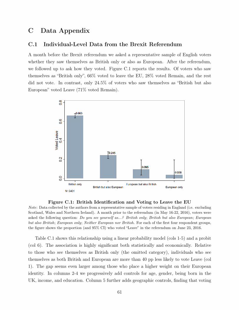
C Data Appendix

C.1 Individual-Level Data from the Brexit Referendum

A month before the Brexit referendum we asked a representative sample of English voterswhether they saw themselves as British only or also as European. After the referendum,we followed up to ask how they voted. Figure C.1 reports the results. Of voters who sawthemselves as “British only”, 66% voted to leave the EU, 28% voted Remain, and the restdid not vote. In contrast, only 24.5% of voters who saw themselves as “British but alsoEuropean” voted Leave (71% voted Remain).

Figure C.1: British Identification and Voting to Leave the EUNote: Data collected by the authors from a representative sample of voters residing in England (i.e. excludingScotland, Wales and Northern Ireland). A month prior to the referendum (in May 16-22, 2016), voters wereasked the following question: Do you see yourself as...? British only ; British but also European; Europeanbut also British; European only ; Neither European nor British. For each of the first four respondent groups,the figure shows the proportion (and 95% CI) who voted “Leave” in the referendum on June 23, 2016.

Table C.1 shows this relationship using a linear probability model (cols 1-5) and a probit(col 6). The association is highly significant both statistically and economically. Relativeto those who see themselves as British only (the omitted category), individuals who seethemselves as both British and European are more than 40 pp less likely to vote Leave (col1). The gap seems even larger among those who place a higher weight on their Europeanidentity. In columns 2-4 we progressively add controls for age, gender, being born in theUK, income, and education. Column 5 further adds geographic controls, finding that voting

61

Table C.1: Voting for Brexit and British/European IdentityProbit

(1) (2) (3) (4) (5) (6)

Identity

British but also European -0.419*** -0.412*** -0.406*** -0.372*** -0.365*** -0.394***(0.021) (0.021) (0.021) (0.022) (0.023) (0.023)

European but also British -0.568*** -0.518*** -0.515*** -0.481*** -0.463*** -0.526***(0.039) (0.044) (0.045) (0.045) (0.046) (0.050)

European only -0.625*** -0.535*** -0.527*** -0.491*** -0.474*** -0.587***(0.039) (0.047) (0.047) (0.049) (0.047) (0.062)

Neither European nor British -0.116** -0.094* -0.105* -0.085 -0.085 -0.080(0.056) (0.054) (0.054) (0.054) (0.053) (0.057)

Age 0.020*** 0.021*** 0.019*** 0.019*** 0.023***(0.004) (0.004) (0.004) (0.004) (0.005)

Age Square -0.000*** -0.000*** -0.000*** -0.000*** -0.000***(0.000) (0.000) (0.000) (0.000) (0.000)

Female -0.025 -0.032* -0.025 -0.032* -0.031(0.018) (0.018) (0.018) (0.019) (0.022)

Born in UK 0.089** 0.090** 0.084** 0.075** 0.121**(0.038) (0.038) (0.037) (0.038) (0.050)

ln(HH Income) -0.038*** -0.020 -0.021 -0.022(0.013) (0.013) (0.013) (0.016)

Education

GSCE, GNQV or equivalent -0.010 -0.004 -0.013(0.044) (0.045) (0.054)

A-Levels or equivalent -0.028 -0.030 -0.029(0.046) (0.046) (0.055)

Professional qualifications 0.026 0.030 0.032(0.048) (0.048) (0.058)

Academic degree -0.146*** -0.138*** -0.166***(0.046) (0.047) (0.055)

County FE No No No No Yes No

Observations 2,485 2,485 2,462 2,462 2,462 2,462R-squared / Pseudo R-squared 0.154 0.187 0.190 0.205 0.224 0.162

*** is significant at 1%; ** is significant at 5%; * is significant at the 10% level.

OLS

Notes: Dependent variable equals 1 if voted "Leave" and 0 if voted "Remain" or did not vote in the Brexit referendum on June 23, 2016. The Identity variable was measured in May 16-22, 2016, the omitted category is "British only". The omitted category for education is no formal qualifications. Column 5 controls for 49 counties. Column 6 reports marginal effects from a probit regression. Robust standard errors in parenthesis.

is strongly associated with British/European identification even within county of residence.Consistent with other studies, older, less-educated, and native voters were more likely tosupport Brexit (see Becker et al., 2017). However, adding variables such as income, age andeducation does not dramatically increase the explanatory power of the regression beyondwhat is explained by the identity variable alone, measured a month before the referendum.14

14Removing the identity variable from columns 4 and 5 produces R2 of 0.0998 and 0.125, respectively.

62

C.2 Joining the European Monetary Union

This appendix briefly explores the composition of the eurozone in light of the model. Focusingon the formation of the eurozone, we compare the predictions of our theory to those of thestandard Optimum Currency Area (OCA) framework which is focused on material costsand benefits alone. The exercise here is exploratory and tentative in nature: a much morethorough empirical investigation is required to disentangle identity from other economicand political effects. Nonetheless, we find that while the standard international integrationframework does not fully explain the composition of the eurozone, augmenting it with identitypolitics can help bridge some of the gap.

The theory of OCA emphasizes three main classes of costs and benefits (see Silva andTenreyro 2010 for a review). First is the difficulty in addressing asymmetric shocks undera common monetary policy (e.g. Mundell (1961); McKinnon (1963); Kenen (1969)). Atthe same time, joining a currency union helps reduce transaction costs and promote trade(Mundell, 1961; Rose and Honohan, 2001). Hence, countries should be more likely to joina currency union the greater the comovement between their business cycles, and the morethey trade with each other (Alesina et al. 2002). Finally, joining a union can help countrieswith limited ability to commit to a monetary rule and thereby overcome the inflation-biasproblem (e.g. Alesina and Barro 2002; Clerc et al. 2011; Aguiar et al. 2015; Chari et al.2020).

We begin by computing empirical measures for the OCA criteria, building on Alesina etal. (2002). Specifically, we look at comovement in prices and in output, as well as trade, forEuropean countries relative to France and Germany (the Core members of the union). Interms of our model, these measures from the OCA literature can also be taken as proxies forfundamental differences in optimal policy, inasmuch as countries for whom it is economicallyoptimal to join a currency union have similar optimal monetary policies. For the most partwe restrict attention to countries that, at least at some point, were members of the EU,which is a prerequisite for joining the euro. For each country i, we compute the correlationcoefficient ρiy between the annual growth rate of real per-capita GDP of that country and thegrowth rate of the combined real per-capita GDP in Germany and France. The correlationis calculated over the period following the reunification of Germany and before the launchof the euro i.e., 1992-1999. Similarly we compute the correlation coefficient ρip between theannual inflation rate of country i and the combined inflation rate in Germany and Franceover the 1992-1999 period. Finally, let Tit be country i’s trade (average of imports andexports) with Germany and France in year t, as a percentage of i’s GDP. Our measure oftrade relations Ti is the average Tit in 1992-1999.

Overall, 19 of the 28 countries that were at some point members of the EU, joined the

63

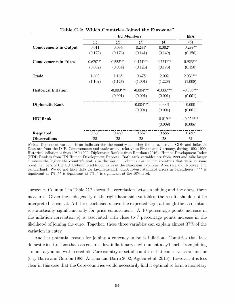
Table C.2: Which Countries Joined the Eurozone?EEA

(1) (2) (3) (4) (5)Comovements in Output 0.011 0.036 0.244* 0.302* 0.299**

(0.172) (0.176) (0.141) (0.149) (0.150)

Comovements in Prices 0.670*** 0.553*** 0.424*** 0.771*** 0.923***(0.082) (0.084) (0.125) (0.173) (0.150)

Trade 1.693 1.165 0.475 2.002 2.931***(1.109) (1.127) (1.001) (1.228) (1.008)

Historical Inflation -0.003*** -0.004*** -0.006*** -0.006***(0.001) (0.001) (0.001) (0.001)

Diplomatic Rank -0.004*** -0.002 0.000(0.001) (0.001) (0.001)

HDI Rank -0.019** -0.026***(0.009) (0.006)

R-squared 0.368 0.460 0.587 0.686 0.692Observations 28 28 28 28 31

EU Members

Notes: Dependent variable is an indicator for the country adopting the euro. Trade, GDP and inflationData are from the IMF. Comovements and trade are all relative to France and Germany, during 1992-1999.Historical inflation is from 1980-1999. Diplomatic Rank is from Renshon (2016). Human Development Index(HDI) Rank is from UN Human Development Reports. Both rank variables are from 1999 and take largernumbers the higher the country’s status in the world. Columns 1-4 include countries that were at somepoint members of the EU. Column 5 adds countries in the European Economic Area (Iceland, Norway, andSwitzerland. We do not have data for Liechtenstein). OLS, robust standard errors in parentheses. *** issignificant at 1%; ** is significant at 5%; * is significant at the 10% level.

eurozone. Column 1 in Table C.2 shows the correlation between joining and the above threemeasures. Given the endogeneity of the right-hand-side variables, the results should not beinterpreted as causal. All three coefficients have the expected sign, although the associationis statistically significant only for price comovement. A 10 percentage points increase inthe inflation correlation ρip is associated with close to 7 percentage points increase in thelikelihood of joining the euro. Together, these three variables can explain almost 37% of thevariation in entry.

Another potential reason for joining a currency union is inflation. Countries that lackdomestic institutions that can ensure a low-inflationary environment may benefit from joininga monetary union with a credible Core country or set of countries that can serve as an anchor(e.g. Barro and Gordon 1983; Alesina and Barro 2002; Aguiar et al. 2015). However, it is lessclear in this case that the Core countries would necessarily find it optimal to form a monetary

64

union with the bad-institutions countries.15 Column 2 in Table C.2 adds the average annualinflation rate between 1980-1999 to proxy for the (lack of) internal discipline in monetarypolicy.16 The results offer little evidence that countries with higher historical inflation weremore likely to join the eurozone: if anything, the association is in the opposite direction.17

Turning to our model, Proposition 7 suggests that low-status countries may join the unionat higher levels of fundamental differences than high-status countries. There is no singleway of quantifying country status, but several measures are readily available. One followsthe convention in the field of International Relations of using diplomatic exchange data toassess country status. Specifically, Renshon (2016) develops a network-centrality measure ofcountry i′s international status, based on the number of diplomats sent to country i, takinginto account the importance (status) of the sending country. This produces a diplomaticranking of countries with larger numbers corresponding to higher status. Countries in ourdata range from 27 to 188. A second (and more intuitive for economists) proxy for countrystatus is its rank in the Human Development Index (HDI), a summary measure of threedimensions: health, education and standard of living. HDI rank in our data ranges from 97to 150. The two rankings are positively—but not perfectly—correlated (ρ = .31).18

Column 3 in Table C.2 adds diplomatic rank. Consistent with Proposition 7, countrieswith higher status according to this measure are significantly less likely to join the euro.Adding the HDI rank in column 4 shows an additional negative effect. Taken together,adding the status variables increases the explanatory power of the regression to R2 = .69.Column 5 further includes countries in the European Economic Area (Iceland, Norway, andSwitzerland) which are not members of the EU, but presumably could easily join and beeligible for the euro. The results are similar.

Notice that while both the diplomatic and the HDI rankings are plausible measures of15See Chari et al. 2020 for an analysis of the conditions where this can benefit the Core countries. In an

influential paper, Fleming (1971) argued that stable and similar inflation rates across countries stabilize theterms of trade. This in turn reduces the likelihood of reducing the incidence of external imbalances and theneed for nominal exchange-rate adjustment. Indeed, this is reflected in one of the conditions for accessionto the euro established in the Maastricht Treaty: A country can join the union only if its inflation rate wereno higher than 1.5 percentage points above the average of the three best-performing member states.

16Following Alesina et al. (2002), we use a 20 year period that precedes the unification process to captureinflation rates that would arise in the absence of a currency union. Using inflation in the 1992-1999 windowyields very similar results.

17Adding the variance of past inflation does not affect the results. Inflation variance itself is very weaklyassociated with joining the euro. Looking within countries over time, section C.3 below finds no clearassociation between gaps in optimal monetary policy and changes in popular support for the euro.

18We use a country’s rank on the HDI to be consistent with the diplomatic rank data. Results arequalitatively similar when using the HDI index. As we discuss in section C.4 below, the HDI and thediplomatic rank measures are also appealing as they can explain over 85% of the variation across Europeancountries in the Best Countries Ranking (BCR) - an elaborate ranking of countries that is only availableafter 2016.

65

Figure C.2: Euro Membership, Fundamental Differences and Status in 1999Notes: EEA member countries. Fundamental differences computed from comovement and trade data for1992-1999. Status computed from HDI and diplomatic rankings for 1999.

status, neither has an obvious counterpart in the OCA framework. For example, whilecomovement of output is important, conditional on that it is not clear how lower levels ofoutput in the periphery affect the optimality of both core and periphery countries enteringinto a currency union. Still, country status is obviously correlated with many other factorsthat could affect the observed association.

Figure C.2 provides a graphic illustration to help see which countries drive the resultsin Table C.2. To do that, we combine the comovement and trade variables into an index offundamental differences from France and Germany. We also combine the two rank variablesinto a single index of country status relative to France and Germany. (details are providedin section C.4 below). The red circles show the initial members of the Eurozone. Consistentwith OCA, this set includes the countries with the lowest difference from the Core (Sloveniawas not a member of the EU until 2004). However, at intermediate levels of fundamentaldifferences, there seems to be some interesting variation. Countries that had high status atthe time—the United Kingdom, Sweden, Denmark—did not join the Eurozone (in Denmark

66

despite closely pegging the Danish Krone to the euro). At the same time, consistent withProposition 7, countries with lower status than these non-joiners, but with similar and evenlarger differences did join (notably Finland and Portugal). Even more interesting is theset of countries that adopted the euro in subsequent years (the pink diamonds in FigureC.2). While high status countries stayed out, most of the joiners in the ensuing years wererelatively high-distance low-status countries in 1999. The patterns are fairly similar whenconditioning on pre-1999 inflation (Figure C.3).

Figure C.3: Eurozone Membership, Fundamental Differences and Status in 1999,Conditional on Inflation in 1980-1999

Note: Fundamental economic differences and status from Table C.3, after controlling for the country’s averageinflation rate 1980-1999. For the following countries, IMF inflation data starts at year t > 1980 and we takethe average inflation from year t to 1999. These countries (and first year t) are: Croatia (1993); CzechRepublic (1996); Latvia (1993); Lithuania (1996); Netherlands (1981); Slovakia (1994); Slovenia (1993).

Turning to identification patterns, Propositions 8 and 9 do not provide sharp predictionsregarding low-status periphery countries. However, Proposition 8b says that in any SIE withbreakup, a high-status Periphery identifies nationally. Figure C.4 shows Eurobarometer datafrom 1999 on whether people in different countries see themselves more as European or asmembers of their nation. Data are available for all members of the EU in 1999. Of course,these surveys are merely suggestive, but high status countries that did not join the union did

67

Figure C.4: National vs. European Identity in EU countries (1999)Note: Eurobarometer data. The figure includes countries that were part of the European Union in 1999,excluding France and Germany. Each bar corresponds to a nationally representative sample. The figure showsthe proportion choosing the first answer from the following question: Do you see yourself as...1.[Nationality]only; 2. [Nationality] and European; 3. European and [Nationality]; 4. European only . The left panelincludes countries with a status index (see Appendix C.4) above the median across all countries, and theright panel those below. Red (black) bars correspond to countries that were (not) part of the Eurozone in1999.

seem to have relatively high levels of national identification compared to European identity.19

Taken together, while a standard international integration framework does not fully ex-plain the composition of the European Monetary Union, augmenting it with identity politicsgoes some way in bridging the gap.

C.3 Changes in Support for the Euro

The patterns in Table C.2 and Figure C.2 are based on cross-country comparisons andmay therefore reflect additional differences between countries that may drive integration

19Unfortunately, at present we do not have revealed-preference measures of social identity as defined in themodel. Furthermore, even in survey data, to the best of our knowledge, there currently exist no measures ofidentification with the Core—which in the European case includes both France and Germany. A French or aGerman citizen saying they identify with “Europe”, may very well refer primarily to the core north Europeancountries. We return to this point in the conclusion.

68

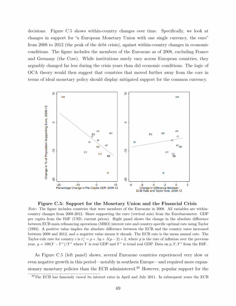
decisions. Figure C.5 shows within-country changes over time. Specifically, we look atchanges in support for “a European Monetary Union with one single currency, the euro”from 2008 to 2012 (the peak of the debt crisis), against within-country changes in economicconditions. The figure includes the members of the Eurozone as of 2008, excluding Franceand Germany (the Core). While institutions surely vary across European countries, theyarguably changed far less during the crisis years than did economic conditions. The logic ofOCA theory would then suggest that countries that moved further away from the core interms of ideal monetary policy should display mitigated support for the common currency.

Figure C.5: Support for the Monetary Union and the Financial CrisisNote: The figure includes countries that were members of the Eurozone in 2008. All variables are within-country changes from 2008-2012. Share supporting the euro (vertical axis) from the Eurobarometer. GDPper capita from the IMF (USD, current prices). Right panel shows the change in the absolute differencebetween ECB main refinancing operations (MRO) interest rate and country-specific optimal rate using Taylor(1993). A positive value implies the absolute difference between the ECB and the country rates increasedbetween 2008 and 2012, and a negative value means it shrank. The ECB rate is the mean annual rate. TheTaylor-rule rate for country i is r∗i = p+ .5y+ .5(p− 2) + 2, where p is the rate of inflation over the previousyear, y = 100(Y −Y ∗)/Y ∗ where Y is real GDP and Y ∗ is trend real GDP. Data on p, Y, Y ∗ from the IMF.

As Figure C.5 (left panel) shows, several Eurozone countries experienced very slow oreven negative growth in this period—notably in southern Europe—and required more expan-sionary monetary policies than the ECB administered.20 However, popular support for the

20The ECB has famously raised its interest rates in April and July 2011. In subsequent years the ECB

69

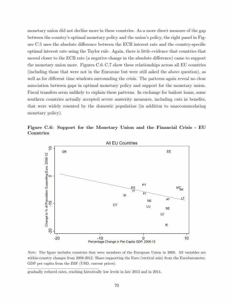
monetary union did not decline more in these countries. As a more direct measure of the gapbetween the country’s optimal monetary policy and the union’s policy, the right panel in Fig-ure C.5 uses the absolute difference between the ECB interest rate and the country-specificoptimal interest rate using the Taylor rule. Again, there is little evidence that countries thatmoved closer to the ECB rate (a negative change in the absolute difference) came to supportthe monetary union more. Figures C.6–C.7 show these relationships across all EU countries(including those that were not in the Eurozone but were still asked the above question), aswell as for different time windows surrounding the crisis. The patterns again reveal no clearassociation between gaps in optimal monetary policy and support for the monetary union.Fiscal transfers seem unlikely to explain these patterns. In exchange for bailout loans, somesouthern countries actually accepted severe austerity measures, including cuts in benefits,that were widely resented by the domestic population (in addition to unaccommodatingmonetary policy).

Figure C.6: Support for the Monetary Union and the Financial Crisis - EUCountries

Note: The figure includes countries that were members of the European Union in 2008. All variables arewithin-country changes from 2008-2012. Share supporting the Euro (vertical axis) from the Eurobarometer.GDP per capita from the IMF (USD, current prices).

gradually reduced rates, reaching historically low levels in late 2013 and in 2014.

70

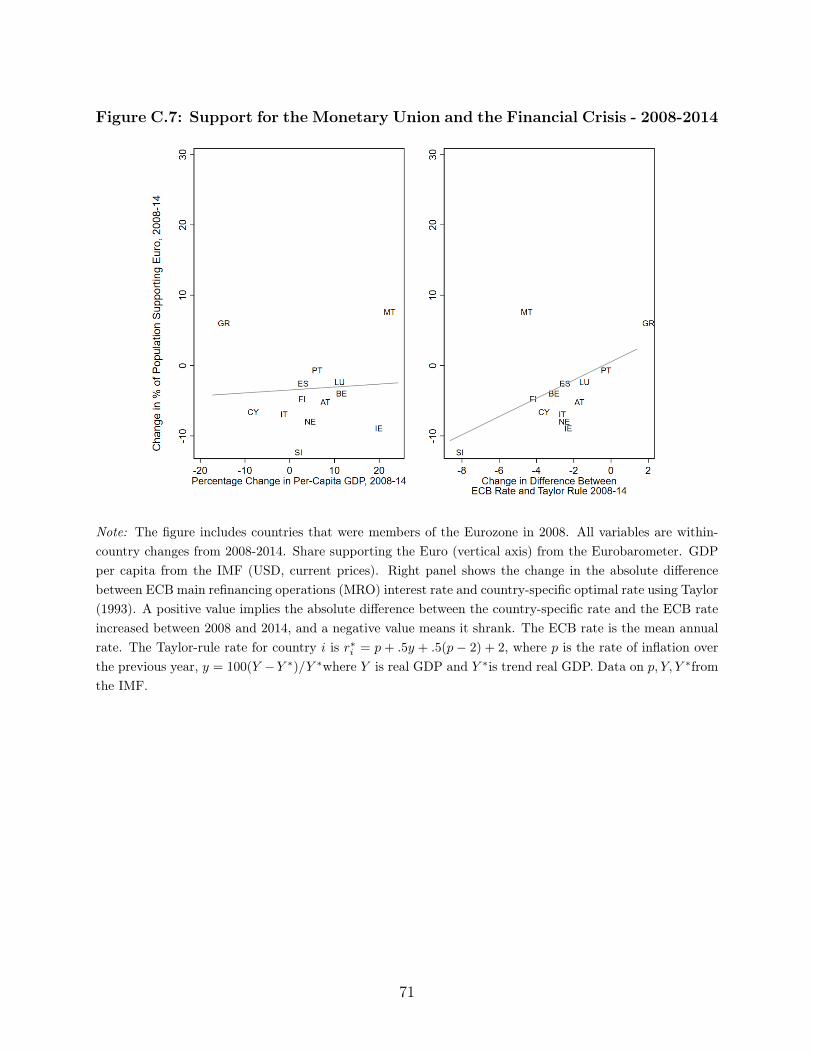
Figure C.7: Support for the Monetary Union and the Financial Crisis - 2008-2014

Note: The figure includes countries that were members of the Eurozone in 2008. All variables are within-country changes from 2008-2014. Share supporting the Euro (vertical axis) from the Eurobarometer. GDPper capita from the IMF (USD, current prices). Right panel shows the change in the absolute differencebetween ECB main refinancing operations (MRO) interest rate and country-specific optimal rate using Taylor(1993). A positive value implies the absolute difference between the country-specific rate and the ECB rateincreased between 2008 and 2014, and a negative value means it shrank. The ECB rate is the mean annualrate. The Taylor-rule rate for country i is r∗i = p+ .5y + .5(p− 2) + 2, where p is the rate of inflation overthe previous year, y = 100(Y −Y ∗)/Y ∗where Y is real GDP and Y ∗is trend real GDP. Data on p, Y, Y ∗fromthe IMF.

71

C.4 Country-Level Data

Constructing summary statistics for fundamental differences and country status

We define the distance in output comovement as δiy = 1−ρiy. Similarly we define the distancein price comovement as δip = 1− ρip. Our measure of distance on the trade dimension is thenδiT rade = 1− Ti.

These measures are reported in Appendix Table C.3. As one way of summarizing thedata, we construct an index of fundamental differences by taking a simple average of thethree differences (δip, δiy, δiT rade), divided by their standard deviation.

For status, An appealing measure of country status is the Best Countries Ranking (BCR)published by U.S. News & World Report.21 This report provides an overall score for eachof the 80 countries studied. It is based on a survey of over 21,000 people from across theglobe who evaluate countries on a list of 65 attributes. The attributes are grouped in ninecategories such as Cultural Influence, Entrepreneurship, Heritage, Openness for Business,Power, and Quality of Life. While BCR scores are not available for 1999 (the year the eurowas launched), the HDI and Renshon’s (2016) international status ranking explain morethan 85% of the variation in BCR across European countries. We can thus use these twoindices from 1999 to impute a status score for each country. Specifically, we regress the BCRscore (normalized to be in [0, 1]) of all available European countries on the country’s HDIranking in 2015 and on Renshon’s (2016) international status ranking in 2005 (the latest dataavailable). This regression has R2 = 85.8.We then use the estimated coefficients to impute aBCR score for 1999. The status of country i relative to the European Core countries (Franceand Germany) is defined as exp(BCR−score)−mean [exp(BCR−score)|Core]. The indicesare reported in Table C.3. Perhaps not surprisingly, Switzerland, the UK and Sweden enjoyvery high status whereas Latvia and Malta have the lowest status within our set of countries.

21The study and model used to score and rank countries were developed by Y&R’sBAV Consulting and David Reibstein of the Wharton School. For details, seehttps://media.beam.usnews.com/ce/e7/fdca61cb496da027ab53bef37a24/171110-best-countries-overall-rankings-2018.pdf. We use the 2017 report, published in March 2017.

72

Table C.3: Fundamental Differences and Status: Europe 1999

Fundamental Differences Status 1999

(4) (6)Belgium 0.91 0.90 0.21 5.70 3.48 0.20Luxembourg 0.90 0.34 0.18 6.27 3.47 -0.51Slovenia 0.95 * 0.69 * 0.14 * 6.27 14.07 * -0.63Austria 0.91 0.88 0.12 6.34 2.95 -0.12Netherlands 0.81 0.71 0.13 6.47 2.24 0.10Ireland 0.94 0.66 0.09 6.63 5.82 -0.39Italy 0.95 0.90 0.05 6.76 7.76 -0.16Denmark 0.91 0.76 0.07 6.77 4.45 -0.05Spain 0.91 0.87 0.06 6.79 7.28 -0.23Latvia 0.93 * 0.82 * 0.06 6.80 28.89 * -0.82Switzerland 0.71 0.68 0.09 6.81 2.81 0.11Sweden 0.87 0.87 0.05 6.86 5.55 0.14Croatia 0.81 * 0.67 * 0.06 * 6.96 233.71 * -0.79Malta 0.36 0.05 0.17 6.99 2.71 -0.82Finland 0.93 0.61 0.05 7.01 4.79 -0.35Portugal 0.61 0.73 0.07 7.03 11.23 -0.47Greece 0.69 0.81 0.03 7.18 15.23 -0.49Cyprus 0.87 0.49 0.03 7.27 4.76 -0.70United Kingdom 0.83 0.36 0.04 7.30 5.14 0.11Lithuania 0.89 **** -0.16 **** 0.08 *** 7.31 9.65 **** -0.79Iceland 0.78 0.34 0.04 7.33 21.45 -0.66Norway 0.78 0.11 0.05 7.44 5.39 -0.08Estonia 0.89 ** -0.36 ** 0.06 * 7.55 19.60 ** -0.79Hungary -0.43 0.65 * 0.12 * 7.59 15.57 -0.58Bulgaria -0.24 0.83 0.08 7.62 95.07 -0.71Czech Republic 0.38 -0.83 **** 0.15 **** 7.64 7.57 -0.40Slovakia 0.35 ** -0.54 ** 0.11 * 7.75 8.73 ** -0.76Poland -0.08 0.21 0.07 7.94 72.35 -0.54Romania -0.29 -0.16 0.05 8.44 62.65 -0.73Mean 0.65 0.44 0.09 7.06 23.60 -0.41SD 0.41 0.47 0.05 0.58 46.18 0.34Columns 1 and 2 show the correlations in annual inflation rate and in annual gdp per-capita growth rate during 1992-1999 betweeneach country and Germany and France (as one combined economy). Column 3 shows trade with France and Germany, as percentageof GDP, in 1992-1999. * = Data available starting in 1993. ** = Data available starting in 1994. *** = Data available starting in 1995.**** = Data available starting in 1996. Column 4 shows the mean of δp, δy, and δTrade, as described in the text. Historical inflationrates (col 5) are computed as the average annual inflation rates between 1980-1999. Columns 1-5 are based on IMF data. Status (col6) is the (exp of) the Best Country Ranking score, relative to the mean of France and Germany, imputed based on 1999 HDI (UNDevelopment Programme) and country status ranking (Renshon 2016).

Comovements in Prices

Comovements in Output

Trade as % of GDP

Pre-1999 Inflation

(1) (2) (3) (5)

73