international journal ofeprints.abuad.edu.ng/100/1/ije_v6_i3.pdf · international journal of...
TRANSCRIPT


INTERNATIONAL JOURNAL OF
ENGINEERING (IJE)
VOLUME 6, ISSUE 3, 2012
EDITED BY
DR. NABEEL TAHIR
ISSN (Online): 1985-2312
International Journal of Engineering is published both in traditional paper form and in Internet.
This journal is published at the website http://www.cscjournals.org, maintained by Computer
Science Journals (CSC Journals), Malaysia.
IJE Journal is a part of CSC Publishers
Computer Science Journals
http://www.cscjournals.org

INTERNATIONAL JOURNAL OF ENGINEERING (IJE)
Book: Volume 6, Issue 3, June 2012
Publishing Date: 20-06-2012
ISSN (Online): 1985-2312
This work is subjected to copyright. All rights are reserved whether the whole or
part of the material is concerned, specifically the rights of translation, reprinting,
re-use of illusions, recitation, broadcasting, reproduction on microfilms or in any
other way, and storage in data banks. Duplication of this publication of parts
thereof is permitted only under the provision of the copyright law 1965, in its
current version, and permission of use must always be obtained from CSC
Publishers.
IJE Journal is a part of CSC Publishers
http://www.cscjournals.org
© IJE Journal
Published in Malaysia
Typesetting: Camera-ready by author, data conversation by CSC Publishing Services – CSC Journals,
Malaysia
CSC Publishers, 2012

EDITORIAL PREFACE
This is the third issue of volume six of International Journal of Engineering (IJE). The Journal is published bi-monthly, with papers being peer reviewed to high international standards. The International Journal of Engineering is not limited to a specific aspect of engineering but it is devoted to the publication of high quality papers on all division of engineering in general. IJE intends to disseminate knowledge in the various disciplines of the engineering field from theoretical, practical and analytical research to physical implications and theoretical or quantitative discussion intended for academic and industrial progress. In order to position IJE as one of the good journal on engineering sciences, a group of highly valuable scholars are serving on the editorial board. The International Editorial Board ensures that significant developments in engineering from around the world are reflected in the Journal. Some important topics covers by journal are nuclear engineering, mechanical engineering, computer engineering, electrical engineering, civil & structural engineering etc. The initial efforts helped to shape the editorial policy and to sharpen the focus of the journal. Starting with volume 6, 2012, IJE appears in more focused issues. Besides normal publications, IJE intend to organized special issues on more focused topics. Each special issue will have a designated editor (editors) – either member of the editorial board or another recognized specialist in the respective field. The coverage of the journal includes all new theoretical and experimental findings in the fields of engineering which enhance the knowledge of scientist, industrials, researchers and all those persons who are coupled with engineering field. IJE objective is to publish articles that are not only technically proficient but also contains information and ideas of fresh interest for International readership. IJE aims to handle submissions courteously and promptly. IJE objectives are to promote and extend the use of all methods in the principal disciplines of Engineering. IJE editors understand that how much it is important for authors and researchers to have their work published with a minimum delay after submission of their papers. They also strongly believe that the direct communication between the editors and authors are important for the welfare, quality and wellbeing of the Journal and its readers. Therefore, all activities from paper submission to paper publication are controlled through electronic systems that include electronic submission, editorial panel and review system that ensures rapid decision with least delays in the publication processes. To build its international reputation, we are disseminating the publication information through Google Books, Google Scholar, Directory of Open Access Journals (DOAJ), Open J Gate, ScientificCommons, Docstoc and many more. Our International Editors are working on establishing ISI listing and a good impact factor for IJE. We would like to remind you that the success of our journal depends directly on the number of quality articles submitted for review. Accordingly, we would like to request your participation by submitting quality manuscripts for review and encouraging your colleagues to submit quality manuscripts for review. One of the great benefits we can provide to our prospective authors is the mentoring nature of our review process. IJE provides authors with high quality, helpful reviews that are shaped to assist authors in improving their manuscripts. Editorial Board Members International Journal of Engineering (IJE)

EDITORIAL BOARD
Editor-in-Chief (EiC)
Dr. Kouroush Jenab
Ryerson University (Canada)
ASSOCIATE EDITORS (AEiCs)
Professor. Ernest Baafi University of Wollongong Australia
Dr. Tarek M. Sobh University of Bridgeport United States of America
Dr. Cheng-Xian (Charlie) Lin University of Tennessee United States of America Assistant Professor Aleksandar Vujovic Univeristy of Montenegro Assistant Professor Jelena Jovanovic University of Montenegro Serbia and Montenegro EDITORIAL BOARD MEMBERS (EBMs)
Professor. Jing Zhang University of Alaska Fairbanks United States of America
Dr. Tao Chen Nanyang Technological University Singapore
Dr. Oscar Hui University of Hong Kong Hong Kong
Professor. Sasikumaran Sreedharan King Khalid University Saudi Arabia
Assistant Professor. Javad Nematian University of Tabriz Iran

Dr. Bonny Banerjee Senior Scientist at Audigence United States of America
AssociateProfessor. Khalifa Saif Al-Jabri Sultan Qaboos University Oman
Dr. Alireza Bahadori Curtin University Australia Dr Guoxiang Liu University of North Dakota United States of America Dr Rosli Universiti Tun Hussein Onn Malaysia Professor Dr. Pukhraj Vaya Amrita Vishwa Vidyapeetham India
Associate Professor Aidy Ali Universiti Putra Malaysia Malaysia Professor Dr Mazlina Esa Universiti Teknologi Malaysia Malaysia Dr Xing-Gang Yan University of Kent United Kingdom Associate Professor Mohd Amri Lajis Universiti Tun Hussein Onn Malaysia Malaysia Associate Professor Tarek Abdel-Salam East Carolina University United States of America Associate Professor Miladin Stefanovic University of Kragujevac Serbia and Montenegro Associate Professor Hong-Hu Zhu Nanjing University China Dr Mohamed Rahayem Örebro University Sweden

Dr Wanquan Liu Curtin University Australia Professor Zdravko Krivokapic University of Montenegro Serbia and Montenegro Professor Qingling Zhang Northeastern University China

International Journal of Engineering (IJE), Volume (6), Issue (3) : 2012
TABLE OF CONTENTS
Volume 6, Issue 3, June 2012
Pages
118 - 128 Development of Dynamic Models for a Reactive Packed Distillation Column
Abdulwahab GIWA & Süleyman KARACAN
129 - 141 Design Baseline Computed Torque Controller
Farzin Piltan, Mina Mirzaei, Forouzan Shahriari, Iman Nazari & Sara Emamzadeh
142 - 177
Sliding Mode Methodology Vs. Computed Torque Methodology Using MATLAB/SIMULINK
and Their Integration into Graduate Nonlinear Control Courses
Farzin Piltan, Sajad Rahmdel, Saleh Mehrara & Reza Bayat
178 – 183 Extremely Low Power FIR Filter for a Smart Dust Sensor Module
Md. Moniruzzaman, Sajib Roy & Md. Murad Kabir Nipun
184 - 200 Optimal Design of Hysteretic Dampers Connecting 2-MDOF Adjacent Structures for Random
Excitations
A. E. Bakeri

Abdulwahab GIWA & Süleyman KARACAN
International Journal of Engineering (IJE), Volume (6) : Issue (3) : 2012 118
Development of Dynamic Models for a Reactive Packed Distillation Column
Abdulwahab GIWA [email protected] Engineering/Chemical Engineering/Process Systems Engineering Ankara University Ankara, 06100, Turkey
Süleyman KARACAN [email protected] Engineering/Chemical Engineering/Process Systems Engineering Ankara University Ankara, 06100, Turkey
Abstract
This work has been carried out to develop dynamic models for a reactive packed distillation column using the production of ethyl acetate as the case study. The experimental setup for the production of ethyl acetate was a pilot scale packed column divided into condenser, rectification, acetic acid feed, reaction, ethanol feed, stripping and reboiler sections. The reaction section was filled with Amberlyst 15 catalyst while the rectification and the stripping sections were both filled raschig rings. The theoretical models for each of the sections of the column were developed from first principles and solved with the aid of MATLAB R2011a. Comparisons were made between the experimental and theoretical results by calculating the percentage residuals for the top and bottom segment temperatures of the column. The results obtained showed that there were good agreements between the experimental and theoretical top and bottom segment temperatures because the calculated percentage residuals were small. Therefore, the developed dynamic models can be used to represent the reactive packed distillation column. Keywords: Reactive Distillation, Dynamic Models, MATLAB, Ethyl Acetate, Percentage Residual.
1. INTRODUCTION There are three main cases in the chemical industry in which combined distillation and chemical reaction occur: (1) use of a distillation column as a chemical reactor in order to increase conversion of reactants, (2) improvement of separation in a distillation column by using a chemical reaction in order to change unfavourable relations between component volatilities, (3) course of parasitic reactions during distillation, decreasing yield of process [1]. Distillation column can be used advantageously as a reactor for systems in which chemical reactions occur at temperatures and pressures suitable to the distillation of components. This combined unit operation is especially useful for those chemical reactions for which chemical equilibrium limits the conversion. By continuous separation of products from reactants while the reaction is in progress, the reaction can proceed to a much higher level of conversion than without separation [1].This phenomenon is referred to as “reactive distillation”. Reactive distillation has been a focus of research in chemical process industry and academia in the last years (e.g., [2]; [3]; [4]; [5]). Combining reaction and distillation has several advantages, including: a) shift of chemical equilibrium and an increase of reaction conversion by simultaneous reaction and separation of products, b) suppression of side reactions and c) utilization of heat of reaction for mass transfer operation. These synergistic effects may result in significant economic

Abdulwahab GIWA & Süleyman KARACAN
International Journal of Engineering (IJE), Volume (6) : Issue (3) : 2012 119
benefits of reactive distillation compared to a conventional design. These economic benefits include: a) lower capital investment, b) lower energy cost and c) higher product yields [6]. Though there are economic benefits of reactive distillation, the combination of both reaction and separation in a single unit has made the design and modelling of the process very challenging. The design issues for reactive distillation (RD) systems are considerably more complex than those involved for either conventional reactors or conventional distillation columns because the introduction of an in situ separation function within the reaction zone leads to complex interactions between vapour-liquid equilibrium, vapour-liquid mass transfer, intra-catalyst diffusion (for heterogeneously catalysed processes) and chemical kinetics. Such interactions have been shown to lead to phenomena of multiple steady states and complex dynamics [7] of the process. In designing a reactive distillation column, the model of the process is required. Broadly speaking, two types of modelling approaches are available in the literature for reactive distillation: the equilibrium stage model and the non-equilibrium stage model [8]. The equilibrium model assumes that the vapour and liquid leaving a stage are in equilibrium. The non-equilibrium model (also known as the “rate-based model”), on the other hand, assumes that the vapour-liquid equilibrium is established only at the interface between the bulk liquid and vapour phases and employs a transport-based approach to predict the flux of mass and energy across the interface. The equilibrium model is mathematically much simpler and computationally less intensive. On the other hand, the non-equilibrium one is more consistent with the real world operations [9]. According to the information obtained from the literature, different studies have been carried out on the two types of models. Noeres et al. (2003) gave a comprehensive overview of basics and peculiarities of reactive absorption and reactive distillation modelling and design. Roat et al. (1986) discussed dynamic simulation of reactive distillation using an equilibrium model. Ruiz et al. (1995) developed a generalized equilibrium model for the dynamic simulation of multicomponent reactive distillation. A simulation package called REActive Distillation dYnamic Simulator (READYS) was used to carry out the simulations. Several test problems were studied and used to compare the work with those of others. Perez-Cisneros et al. (1996) proposed a different approach to the equilibrium model by using chemical elements rather than the real components. Alejski and Duprat (1996) developed a dynamic equilibrium model for a tray reactive distillation column. A similar dynamic equilibrium model was developed by Sneesby et al. (1998) for a tray reactive distillation column for the production of ethyl tert-butyl ether (ETBE). In their work, chemical equilibrium on all the reactive stages and constant enthalpy were assumed to simplify the model. The model was implemented in SpeedUp and simulated. Kreul et al. (1998) developed a dynamic rate-based model for a reactive packed distillation column for the production of methyl acetate. All the important dynamic changes except the vapour holdup were considered in the model developed in their study. The dynamic rate-based model was implemented into the ABACUSS large-scale equation-based modelling environment. Dynamic experiments were carried out and the results were compared to the simulation results. Baur et al. (2001) proposed a dynamic rate-based cell model for reactive tray distillation columns. Both the liquid and vapour phases were divided into a number of contacting cells and the Maxwell–Stefan equations were used to describe mass transfer. Liquid holdup, vapour holdup, and energy holdup were all included in the model. A reactive distillation tray column for the production of ethylene glycol was used to carry out dynamic simulations. Vora and Daoutidis (2001) studied the dynamics and control of a reactive tray distillation column for the production of ethyl acetate from acetic acid and ethyl alcohol. Schneider et al. (2001) studied reactive batch distillation for a methyl acetate system, using a two-film dynamic rate-based model. In their study, pilot plant batch experiments were carried out to validate the dynamic model and the agreement was found to be reasonable. Peng et al. (2003) developed dynamic rate-based and equilibrium models for a reactive packed distillation column for the production of tert-amyl methyl ether (TAME). The two types of models, consisting of differential and algebraic equations, were implemented in gPROMS and dynamic simulations were carried out to study the dynamic behaviour of the reactive distillation of the TAME system.
Abdulwahab GIWA & Süleyman KARACAN
International Journal of Engineering (IJE), Volume (6) : Issue (3) : 2012 120
Heterogeneous reactive distillation in packed towers is of special interest because the catalyst does not have to be removed from the product and different reactive and non-reactive sections can be realized. At the same time, the interactions of reaction and separation increase the complexity of the process and, thus, a better understanding of the process dynamics is required [20]. Therefore, this work is aimed to develop dynamic models for a heterogeneous reactive packed distillation column using the production of ethyl acetate (desired product) and water (by-product) from the esterification reaction between acetic acid and ethanol as the case study. 2. PROCEDURES The procedures used for the accomplishment of this work are divided into two, namely experimental procedure and modelling procedure. 2.1 Experimental Procedure The experimental pilot plant in which the experiments were carried out was a reactive packed distillation column (RPDC) set up as shown in Figures 1a (pictorially) and b (sketch view) below. The column had, excluding the condenser and the reboiler, a height of 1.5 m and a diameter of 0.05 m. The column consisted of a cylindrical condenser of diameter and height of 5 and 22.5 cm respectively. The main column section of the plant was divided into three subsections of approximately 0.5 m each. The upper, middle and lower sections were the rectifying, the reaction and the stripping sections respectively. The rectifying and the stripping sections were packed with raschig rings while the reaction section was filled with Amberlyst 15 solid catalyst (the catalyst had a surface area of 5300 m2/kg, a total pore volume of 0.4 cc/g and a density of 610 kg/m3). The reboiler was spherical in shape and had a volume of 3 Litre. The column was fed with acetic acid at the top (between the rectifying section and the reaction section) while ethanol was fed at the bottom (between the reaction section and the stripping section) with the aid of peristaltic pumps that were operated with the aid of a computer via MATLAB/Simulink program. All the signal inputs (reflux ratio (R), feed ratio (F) and reboiler duty (Q)) to the column and the measured outputs (top segment temperature (Ttop), reaction segment temperature (Trxn) and bottom segment temperature (Tbot)) from the column were sent and recorded respectively on-line with the aid of MATLAB/Simulink computer program and electronic input-output (I/O) modules that were connected to the equipment and the computer system. The esterification reaction, for the production of ethyl acetate and water, taking place in the column is given as shown in Equation (1):
OHHCOOCCHOHHCCOOHCH eqK
2523523 + →←+ (1) The conditions used for the implementation of the experiment of this study are as tabulated below. TABLE 1: Conditions for the experimental study
Parameter Value
Reflux ratio (R) 3
Acetic acid flow rate (Fa), cm3/min 10
Ethanol flow rate (Fe), cm3/min 10
Reboiler duty (Qreb), W 630 It can be seen from Table 1 above that the feed ratio was chosen to be 1 (volume basis) for the experimental study of this particular work.

Abdulwahab GIWA & Süleyman KARACAN
International Journal of Engineering (IJE), Volume (6) : Issue (3) : 2012 121
FIGURE 1: Reactive packed distillation pilot plant: (a) Pictorial view; (b) Sketch view 2.2 Modelling Procedure The development of the models of the reactive packed distillation column of this work was carried out using first principles approach. That is, the models developed were theoretical ones. 2.2.1 Assumptions In the course of developing the theoretical models for the reactive packed distillation column, the following assumptions were made:
i. Occurrence of proper mixing at each stage. ii. Equilibrium condenser, reboiler and feed stages. iii. Constant vapour flow in the column. iv. Constant total molar hold-up at each stage. v. Constant liquid flow at each section.
2.2.2 Model Equations
For the condenser section, that is, for 1=j ,
( )
j
jRdjjj
M
xLLyV
dt
dx +−=
++ 11 (2)
For the rectifying section, that is, for 1:2 −= fanj , for the liquid phase,
( )
−−
∂
∂=
∂
∂jjcy
j
j
j
yyaAkz
xL
Mt
x *'
1 (3)
and for the vapour phase,
( )jj
j
cyjyy
V
aAk
z
y−=
∂
∂* (4)
For the acetic acid feed section, that is, for fanj = ,
(a) (b)

Abdulwahab GIWA & Süleyman KARACAN
International Journal of Engineering (IJE), Volume (6) : Issue (3) : 2012 122
j
jjjjfaajjjjj
M
yVxLxFyVxL
dt
dx −−++=
++−− 1111 (5)
For the reaction section, that is, for 1:1 −+= fefa nnj , for the liquid phase,
( )
+−−
∂
∂=
∂
∂jjjjcy
j
j
j
jWryyaAk
z
xL
Mt
x'*
'
1 (6)
and for the vapour phase,
( )jj
j
cyjyy
V
aAk
z
y−=
∂
∂* (7)
For the ethanol feed section, for fenj = ,
j
jjjjfeejjjjj
M
yVxLxFyVxL
dt
dx −−++=
++−− 1111 (8)
For the stripping section, that is, for 1:1 −+= nnj fe , for the liquid phase,
( )
−−
∂
∂=
∂
∂jjcy
j
j
j
jyyaAk
z
xL
Mt
x *'
1 (9)
and for the vapour phase,
( )jj
j
cyjyy
V
aAk
z
y−=
∂
∂* (10)
For the reboiler section, that is, for nj = ,
j
jjjjjjj
M
yVxLxL
dt
dx −−=
−− 11 (11)
The equilibrium relationships for any concerned stage are also given as:
iii xKy = (12)
11
=∑=
m
i
iy (13)
11
=∑=
m
i
ix (13)
Since the model equations developed in this work for the reactive packed distillation column composed of both ordinary and partial differential equations, the partial differential equations were converted to ordinary differential equations using the backward difference approach, as found in Fausett (2003), to make the model equations uniform in nature. The resulting ordinary differential equations were then solved using the ode15s command of MATLAB R2011a.

Abdulwahab GIWA & Süleyman KARACAN
International Journal of Engineering (IJE), Volume (6) : Issue (3) : 2012 123
3. RESULTS AND DISCUSSIONS In this study, the temperature and compositions of the top segment were taking as the points of interest because they were the ones used to determine the nature of the desired product (ethyl acetate) obtained, but the temperature of the bottom segment was also considered in validating the developed model equations. However, due to the fact the compositions of the mixture could not be measured on-line while performing the experiments, the quality of the top product was inferred from the top temperature. Using the conditions shown in Table 1 to carry out experiments in the pilot plant shown in Figure 1, the dynamics of the process was studied experimentally and it was revealed from the experiment that the steady state top segment temperature was 76.52 oC. The steady state temperature of the bottom segment was also obtained from the experimental dynamics to be 91.96 oC. Using the same data (Table 1) used for the experimental study to simulate the developed model equations with the aid of MATLAB R2011a, the dynamic responses obtained for the top segment and the bottom segment compositions as well as the steady state temperature and composition profiles of the column are as shown in Figures 2 – 5 below. Figure 2 shows the dynamic responses of the mole fractions of components in the top segment of the column and Figure 3 shows that of the mole fractions of the components in the bottom segment. As can be seen from Figure 2, the dynamic response of the mole fraction of ethyl acetate tended towards unity in the condenser while those of the other components were very negligible there.
0 2000 4000 6000 8000 10000 12000 14000 160000
0.1
0.2
0.3
0.4
0.5
0.6
0.7
0.8
0.9
Time (sec)
Liqu
id m
ole
frac
tion
Acetic acidEthanolEthyl AcetateWater
FIGURE 2: Theoretical dynamic responses of mole fractions of components in the condenser Considering Figure 3, it was discovered that the mole fraction of ethyl acetate was low in the reboiler compared to the one present in the condenser. This is an indication that good reaction conversion and separation occurred in the column. Apart from the ethyl acetate that was present in the reboiler, it was also discovered that there were some acetic acid and ethanol still present there too. The reason for the presence of these two components (acetic acid and ethanol) in the reboiler was due to the fact that acetic acid, after being fed into the column at the acetic acid feed section, was moving down the column towards the reboiler while ethanol, being more volatile, was finding its way upwards and the two reactants were meeting at the reaction section where the reaction was taking place. The unreacted portions of these two reactants were definitely

Abdulwahab GIWA & Süleyman KARACAN
International Journal of Engineering (IJE), Volume (6) : Issue (3) : 2012 124
moving downwards to the reboiler and settling there before they were boiled to move up again as a mixed vapour. It was also discovered that the presence of acetic acid and ethanol in the reboiler gave rise to the occurrence of reaction there too. That is to say that the reboiler also served, to some extent, as a reactor in a reactive distillation process.
0 2000 4000 6000 8000 10000 12000 14000 16000
0.05
0.1
0.15
0.2
0.25
0.3
0.35
0.4
0.45
Time (sec)
Liqu
id m
ole
frac
tion
Acetic acidEthanolEthyl AcetateWater
FIGURE 3: Theoretical dynamic responses of mole fraction of components in the reboiler Figures 4 and 5 show the steady-state temperature and composition profiles respectively. As can be seen from Figure 4, the temperature profile tended to be constant from the condenser down the column up to the reaction section where a sharp increase in the temperature was observed. The reason for the increase in the temperature at this section was as a result of the exothermic nature of the reaction taking place at the section. However, for the ethanol feed section, due to the fact that ethanol was fed at room temperature into the column, there was a slight decrease in the temperature of the segment near the point where it (the ethanol) was fed into the column.
Cond 1 2 3 4 5 6 7 8 9 10 11 12 13 14 15 16 17 Reb
78
80
82
84
86
88
Segment
Tem
pera
ture
( o C
)
FIGURE 4: Steady state temperature profile obtained from the simulation of theoretical models

Abdulwahab GIWA & Süleyman KARACAN
International Journal of Engineering (IJE), Volume (6) : Issue (3) : 2012 125
It is worth mentioning at this point that no such decrease in temperature was witnessed in the case of acetic acid feed segment owing to the fact the heat liberated from the reaction and the heat carried by the vapour moving upward was able to counter the decreasing effect that the acetic acid feed fed into the column at room temperature might have had on the temperature profile of the column. The temperature profile was also noticed to be approximately constant in the stripping section but later increased towards the reboiler section where the maximum temperature of the column was observed. All in all, the steady state temperatures of the top and bottom segments estimated from the dynamic simulation of the theoretical models were found to be 77.33 and 89.22 oC respectively. Also obtained from the simulation of the theoretical models were the composition profiles shown in Figure 5 below. As can be seen from the figure, the steady state mole fraction of the desired product (ethyl acetate) from the liquid obtained at the top segment of the column was discovered to be 0.9963. It is a motivating result having almost pure ethyl acetate as the top product theoretically, especially if the theoretical models are able to represent the real plant very well.
Cond 1 2 3 4 5 6 7 8 9 10 11 12 13 14 15 16 17 Reb0
0.1
0.2
0.3
0.4
0.5
0.6
0.7
0.8
0.9
Segment
Liqu
id m
ole
frac
tion
Acetic acidEthanolEthyl AcetateWater
FIGURE 5: Steady state composition profiles obtained from the simulation of theoretical models
In order to know how well the developed models could represent the plant, comparisons between the experimental and the theoretical top and bottom segment temperatures of the column were made as shown in Table 2 below. It was observed from the results, as can be seen from the table, that good agreements existed between the experimental and the theoretical results because the percentage absolute residual of the top segment temperatures was calculated to be 1.06% while that of the bottom segment temperature was also calculated to be 2.98%. The percentage residuals were found to be low enough to say that the developed theoretical model is a good representation of the reactive packed distillation column. TABLE 2: Comparisons between experimental and theoretical temperatures
Description Values
Top Segment Bottom Segment
Experimental temperature (oC) 76.52 91.96
Theoretical temperature (oC) 77.33 89.22
Absolute residual (oC) 0.81 2.74
Percentage absolute residual (%) 1.06 2.98

Abdulwahab GIWA & Süleyman KARACAN
International Journal of Engineering (IJE), Volume (6) : Issue (3) : 2012 126
4. CONCLUSIONS The results obtained from this study have shown there were good agreements between the top and bottom segment temperatures estimated from the experimental study and the one obtained from the simulation of the theoretical models developed for the reactive packed distillation column because their percentage absolute residuals were less than 5.00% that was set as the criterion for the validity of the model equations. Therefore, the developed models have been found to be suitable in representing the reactive packed distillation column very well. 5. NOMENCLATURES Symbols Ac Column cross sectional area (m2) Acat Catalyst specific surface area (m2/kg) Cp Specific heat capacity (J/(kmol K)) F Feed ratio (mL s-1 acetic acid/mL s-1 ethanol) Fa Acetic acid feed molar rate (kmol/s) Fe Ethanol feed molar rate (kmol/s) K Phase equilibrium constant Keq Equilibrium reaction rate constant kya Mass transfer coefficient (kmol/(m2 s)) L Liquid molar flow rate (kmol/s) M Molar hold up (kmol) M’ Molar hold per segment (kmol/m) Q Reboiler duty (kJ/s) r' Reaction rate (kmol/(kg s)) R Reflux ratio (kmol s-1 recycled liquid / kmol s-1 distillate) t Time (s) T Temperature (oC) V Vapor molar flow rate (kmol/s) W Catalyst weight (kgcat) x Liquid mole fraction y Vapor mole fraction z Flow length (m) Abbreviations MATLAB Matrix Laboratory RPDC Reactive Packed Distillation Column Subscripts a Acetic acid cat Catalyst e Ethanol fa Acetic acid feed fe Ethanol feed i Component j Column segment L Liquid phase m Component number n Segment number Superscript * Equilibrium 6. ACKNOWLEDGEMENTS Abdulwahab GIWA wishes to acknowledge the support received from The Scientific and Technological Research Council of Turkey (TÜBĐTAK) for his PhD Programme. In addition, this

Abdulwahab GIWA & Süleyman KARACAN
International Journal of Engineering (IJE), Volume (6) : Issue (3) : 2012 127
research was supported by Ankara University Scientific Research Projects under the Project No 09B4343007. 7. REFERENCES
[1] K. Alejski, F. Duprat. “Dynamic simulation of the multicomponent reactive distillation”. Chemical Engineering Science, 51(18): 4237 4252, 1996.
[2] V.H. Agreda, L. R. Partin and W.H. Heise. “High purity methyl acetate via reactive
distillation”. Chemical Engineering Progress, 86(2): 40-46, 1990. [3] D. Barbosa, M.F. Doherty. “The simple distillation of homogeneous reactive mixtures”.
Chemical Engineering Science, 43: 541-550, 1988. [4] B. Bessling, G. Schembecker and K.H. Simmrock. “Design of processes with reactive
distillation line diagrams”. Industrial and Engineering Chernistry Research, 36: 3032-3042, 1997.
[5] B. Bessling, J.M. Loning, A. Ohligschläger, G. Schembecker and K. Sundmacher.
“Investigations on the synthesis of methyl acetate in a heterogeneous reactive distillation process”. Chemical Engineering Technology, 21: 393-400, 1998.
[6] P. Moritz, H. Hasse. “Fluid dynamics in reactive distillation packing Katapak®-S”. Chemical
Engineering Science, 54: 1367-1374, 1999. [7] R. Baur, R. Taylor and R. Krishna. “Development of a dynamic nonequilibrium cell model
for reactive distillation tray columns”. Chemical Engineering Science, 55: 6139-6154, 2000. [8] R. Baur, A.P. Higler, R. Taylor and R. Krishna. “Comparison of equilibrium stage and
nonequilibrium stage models for reactive distillation”. Chemical Engineering Journal, 76: 33–47, 2000.
[9] A.M. Katariya, R.S. Kamath, S. M. Mahajani and K.M. Moudgalya. “Study of Non-linear
dynamics in Reactive Distillation for TAME synthesis using Equilibrium and Non-equilibrium models”. In Proceedings of the 16th European Symposium on Computer Aided Process Engineering and 9th International Symposium on Process Systems Engineering. Garmisch-Partenkirchen, Germany, 2006.
[10] C. Noeres, E.Y. Kenig and A. Górak. “Modelling of reactive separation processes: reaction
absorption and reactive distillation”. Chemical Engineering and Processing, 42: 157-178, 2003.
[11] S.D. Roat, J. J. Downs, E.F. Vogel and J.E. Doss. “The integration of rigorous dynamic
modeling and control system synthesis for distillation columns: An industrial approach.” In M. Morari, & T. J. McAvoy, Chemical process control, CPC III. New York: Elsevier. 1986.
[12] C.A. Ruiz, M.S. Basualdo and N.J. Scenna. “Reactive distillation dynamic simulation”.
Chemical Engineering Research and Design, Transactions of the Institution of Chemical Engineers, Part A, 73: 363-378, 1995.
[13] S. Pérez-Correa, P. González and J. Alvarez. “On-line optimizing control for a class of
batch reactive distillation columns”. In Proceedings of the 17th World Congress the International Federation of Automatic Control. Seoul, Korea, 2008
[14] M.G. Sneesby, M.O. Tade and T.N. Smith. “Steady-state transitions in the reactive
distillation of MTBE”. Computers and Chemical Engineering, 22(7-8): 879-892, 1998.

Abdulwahab GIWA & Süleyman KARACAN
International Journal of Engineering (IJE), Volume (6) : Issue (3) : 2012 128
[15] L.U. Kreul, A. Górak, C. Dittrich, and P.I. Barton. “Dynamic Catalytic Distillation: Advanced
Simulation and Experimental Validation”. Computers and Chemical Engineering, 22: 371-378, 1998.
[16] R. Baur R. Taylor and R. Krishna. “Dynamic behaviour of reactive distillation tray columns
described with a nonequilibrium cell model”. Chemical Engineering Science, 56: 1721-1729, 2001.
[17] N. Vora, P. Daoutidis. “Dynamics and control of an ethyl acetate reactive distillation
column”. Industrial and Engineering Chemistry Research, 40: 833-849, 2001. [18] R. Schneider, C. Noeres, L.U. Kreul and A. Górak. “Dynamic modeling and simulation of
reactive batch distillation”. Computers and Chemical Engineering, 25: 169–176, 2001. [19] J. Peng, T.F. Edgar and R.B. Eldridge. “Dynamic rate-based and equilibrium models for a
packed reactive distillation column”. Chemical Engineering Science, 58: 2671-2680, 2003. [20] F. Forner, M. Meyer, M. Döker, J. Repke, J. Gmehling and G. Wozny. “Comparison of the
startup of reactive distillation in packed and tray towers”. In Proceedings of the 16th European Symposium on Computer Aided Process Engineering and 9th International Symposium on Process Systems Engineering. Garmisch-Partenkirchen, Germany, 2006.
[21] L.V. Fausett. Numerical Methods: Algorithms and Applications. Pearson Education, Inc.,
2003, pp. 407-443.

Farzin Piltan, Mina Mirzaei, Forouzan Shahriari, Iman Nazari & Sara Emamzadeh
International Journal of Engineering (IJE), Volume (6) : Issue (3) : 2012 129
Design Baseline Computed Torque Controller
Farzin Piltan [email protected] Industrial Electrical and Electronic Engineering SanatkadeheSabze Pasargad. CO (S.S.P. Co), NO:16 ,PO.Code 71347-66773, Fourth floor Dena Apr , Seven Tir Ave , Shiraz , Iran
Mina Mirzaei [email protected] Industrial Electrical and Electronic Engineering SanatkadeheSabze Pasargad. CO (S.S.P. Co), NO:16 ,PO.Code 71347-66773, Fourth floor Dena Apr , Seven Tir Ave , Shiraz , Iran
Forouzan Shahriari [email protected] Industrial Electrical and Electronic Engineering SanatkadeheSabze Pasargad. CO (S.S.P. Co), NO:16 ,PO.Code 71347-66773, Fourth floor Dena Apr , Seven Tir Ave , Shiraz , Iran
Iman Nazari [email protected] Industrial Electrical and Electronic Engineering SanatkadeheSabze Pasargad. CO (S.S.P. Co), NO:16 ,PO.Code 71347-66773, Fourth floor Dena Apr , Seven Tir Ave , Shiraz , Iran
Sara Emamzadeh [email protected] Industrial Electrical and Electronic Engineering SanatkadeheSabze Pasargad. CO (S.S.P. Co), NO:16 ,PO.Code 71347-66773, Fourth floor Dena Apr , Seven Tir Ave , Shiraz , Iran
Abstract
The application of design nonlinear controller such as computed torque controller in control of 6 degrees of freedom (DOF) robot arm will be investigated in this research. One of the significant challenges in control algorithms is a linear behavior controller design for nonlinear systems (e.g., robot manipulator). Some of robot manipulators which work in industrial processes are controlled by linear PID controllers, but the design of linear controller for robot manipulators is extremely difficult because they are hardly nonlinear and uncertain. To reduce the above challenges, the nonlinear robust controller is used to control of robot manipulator. Computed torque controller is a powerful nonlinear controller under condition of partly uncertain dynamic parameters of system. This controller is used to control of highly nonlinear systems especially for robot manipulators. To adjust this controller’s coefficient baseline methodology is used and applied to CTC. Keywords: Baseline Tuning Computed Torque Controller, Computed Torque Controller, Unstructured Model Uncertainties, Adaptive Method.
Farzin Piltan, Mina Mirzaei, Forouzan Shahriari, Iman Nazari & Sara Emamzadeh
International Journal of Engineering (IJE), Volume (6) : Issue (3) : 2012 130
1. INTRODUCTION and MOTIVATION PUMA 560 robot manipulator is a 6 DOF serial robot manipulator. From the control point of view, robot manipulator divides into two main parts i.e. kinematics and dynamic parts. Controller is a device which can sense information from linear or nonlinear system (e.g., robot manipulator) to improve the systems performance [1-4]. The main targets in designing control systems are stability, good disturbance rejection, and small tracking error[5-6]. Several industrial robot manipulators are controlled by linear methodologies (e.g., Proportional-Derivative (PD) controller, Proportional- Integral (PI) controller or Proportional- Integral-Derivative (PID) controller), but when robot manipulator works with various payloads and have uncertainty in dynamic models this technique has limitations. In some applications robot manipulators are used in an unknown and unstructured environment, therefore strong mathematical tools used in new control methodologies to design nonlinear robust controller with an acceptable performance (e.g., minimum error, good trajectory, disturbance rejection). Computed torque controller (CTC) is an influential nonlinear controller to certain systems which it is based on feedback linearization and computes the required arm torques using the nonlinear feedback control law. When all dynamic and physical parameters are known the controller works superbly; practically a large amount of systems have uncertainties and sliding mode controller reduce this kind of limitation [7]. This controller is used to control of highly nonlinear systems especially for robot manipulators. In various dynamic parameters systems that need to be training on-line adaptive control methodology is used.
Background Computed torque controller (CTC) is a powerful nonlinear controller which it widely used in control robot manipulator. It is based on Feed-back linearization and computes the required arm torques using the nonlinear feedback control law. This controller works very well when all dynamic and physical parameters are known but when the robot manipulator has variation in dynamic parameters, in this situation the controller has no acceptable performance[14]. In practice, most of physical systems (e.g., robot manipulators) parameters are unknown or time variant, therefore, computed torque like controller used to compensate dynamic equation of robot manipulator[1, 6]. Research on computed torque controller is significantly growing on robot manipulator application which has been reported in [1, 6, 15-16]. Vivas and Mosquera [15]have proposed a predictive functional controller and compare to computed torque controller for tracking response in uncertain environment. However both controllers have been used in Feed-back linearization, but predictive strategy gives better result as a performance. A computed torque control with non parametric regression models have been presented for a robot arm[16]. This controller also has been problem in uncertain dynamic models. Based on [1, 6]and [15-16]Computed torque controller is a significant nonlinear controller to certain systems which it is based on feedback linearization and computes the required arm torques using the nonlinear feedback control law. When all dynamic and physical parameters are known the controller works fantastically; practically a large amount of systems have uncertainties and sliding mode controller decrease this kind of challenge.
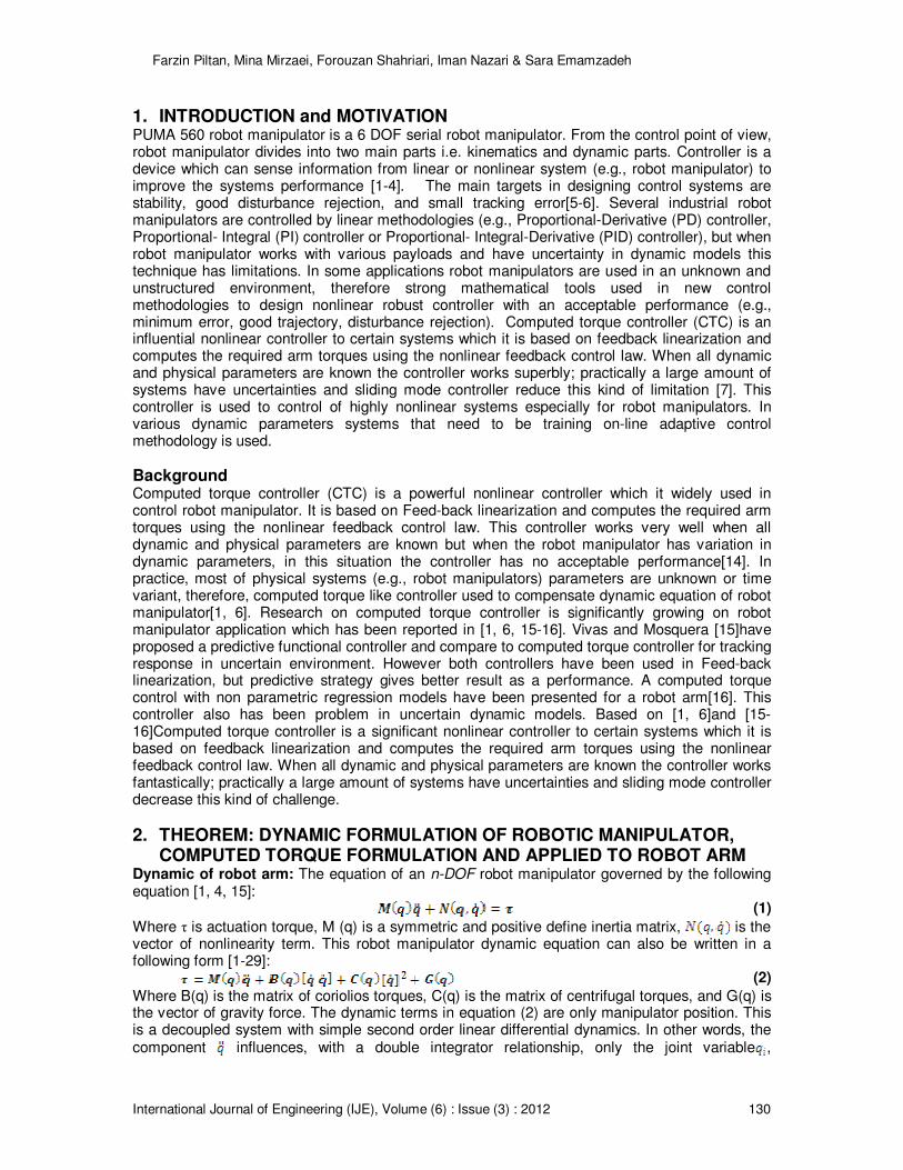
2. THEOREM: DYNAMIC FORMULATION OF ROBOTIC MANIPULATOR,
COMPUTED TORQUE FORMULATION AND APPLIED TO ROBOT ARM Dynamic of robot arm: The equation of an n-DOF robot manipulator governed by the following equation [1, 4, 15]:
(1)
Where τ is actuation torque, M (q) is a symmetric and positive define inertia matrix, is the vector of nonlinearity term. This robot manipulator dynamic equation can also be written in a following form [1-29]:
(2)
Where B(q) is the matrix of coriolios torques, C(q) is the matrix of centrifugal torques, and G(q) is the vector of gravity force. The dynamic terms in equation (2) are only manipulator position. This is a decoupled system with simple second order linear differential dynamics. In other words, the component influences, with a double integrator relationship, only the joint variable ,
Farzin Piltan, Mina Mirzaei, Forouzan Shahriari, Iman Nazari & Sara Emamzadeh
International Journal of Engineering (IJE), Volume (6) : Issue (3) : 2012 131
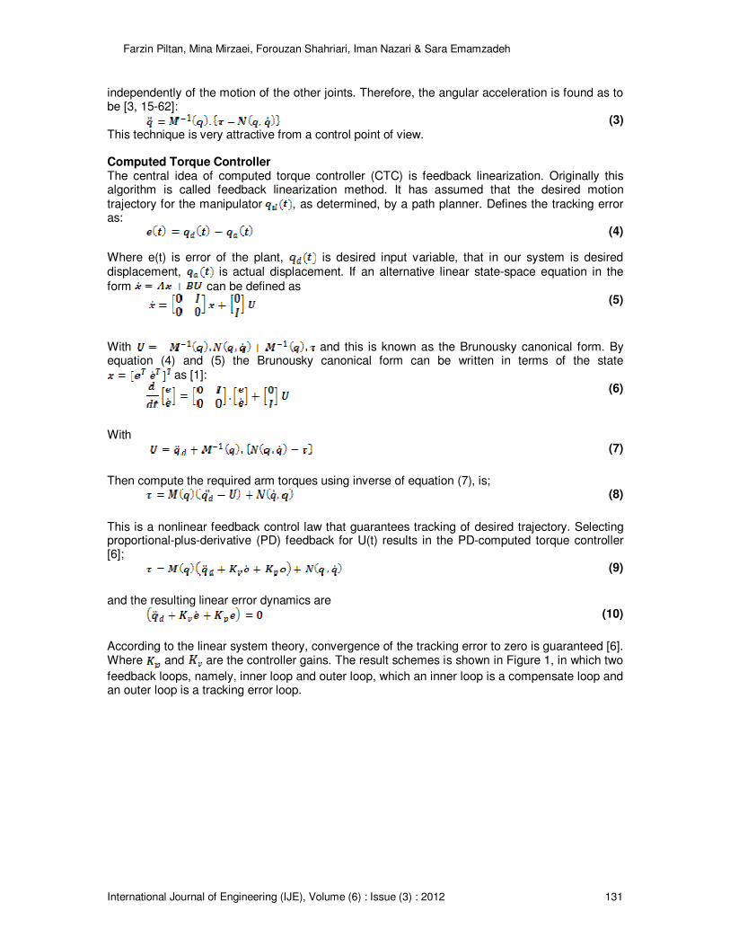
independently of the motion of the other joints. Therefore, the angular acceleration is found as to be [3, 15-62]:
(3)
This technique is very attractive from a control point of view. Computed Torque Controller The central idea of computed torque controller (CTC) is feedback linearization. Originally this algorithm is called feedback linearization method. It has assumed that the desired motion trajectory for the manipulator , as determined, by a path planner. Defines the tracking error as:
(4)
Where e(t) is error of the plant, is desired input variable, that in our system is desired displacement, is actual displacement. If an alternative linear state-space equation in the
form can be defined as
(5)
With and this is known as the Brunousky canonical form. By equation (4) and (5) the Brunousky canonical form can be written in terms of the state
as [1]:
(6)
With
(7)
Then compute the required arm torques using inverse of equation (7), is;
(8)
This is a nonlinear feedback control law that guarantees tracking of desired trajectory. Selecting proportional-plus-derivative (PD) feedback for U(t) results in the PD-computed torque controller [6];
(9)
and the resulting linear error dynamics are
(10)
According to the linear system theory, convergence of the tracking error to zero is guaranteed [6]. Where and are the controller gains. The result schemes is shown in Figure 1, in which two
feedback loops, namely, inner loop and outer loop, which an inner loop is a compensate loop and an outer loop is a tracking error loop.

Farzin Piltan, Mina Mirzaei, Forouzan Shahriari, Iman Nazari & Sara Emamzadeh
International Journal of Engineering (IJE), Volume (6) : Issue (3) : 2012 132
FIGURE 1: Block diagram of PD-computed torque controller (PD-CTC)
The application of proportional-plus-derivative (PD) computed torque controller to control of PUMA 560 robot manipulator introduced in this part. Suppose that in (9) the nonlinearity term defined by the following term;
(11)
Therefore the equation of PD-CTC for control of PUMA 560 robot manipulator is written as the equation of (12);
(12)
The controller based on a formulation (12) is related to robot dynamics therefore it has problems in uncertain conditions.

Farzin Piltan, Mina Mirzaei, Forouzan Shahriari, Iman Nazari & Sara Emamzadeh
International Journal of Engineering (IJE), Volume (6) : Issue (3) : 2012 133
3. METHODOLOGY: BASELINE ON-LINE TUNING FOR STABLE COMPUTED TORQUE CONTROLLER
Computed torque controller has difficulty in handling unstructured model uncertainties. It is possible to solve this problem by combining CTC and baseline tuning method which this method can helps to improve the system’s tracking performance by online tuning method. In this research the nonlinear equivalent dynamic (equivalent part) formulation problem in uncertain system is solved by using on-line linear error-based tuning theorem. In this method linear theorem is applied to CTC to adjust the coefficient. CTC has difficulty in handling unstructured model uncertainties and this controller’s performance is sensitive to controller coefficient. It is possible to solve above challenge by combining linear error-based tuning method and CTC. Based on above discussion, compute the best value of controller coefficient has played important role to improve system’s tracking performance especially when the system parameters are unknown or uncertain. This problem is solved by tuning the controller coefficient of the CTC continuously in real-time. In this methodology, the system’s performance is improved with respect to the pure CTC. Figure 2 shows the baseline tuning CTC. Based on (23) and (27) to adjust the controller
coefficient we define as the baseline tuning.
FIGURE 2: Block diagram of a baseline computed torque controller
(13)
If minimum error ( ) is defined by;
(14)
Where is adjusted by an adaption law and this law is designed to minimize the error’s
parameters of adaption law in linear error-based tuning CTC is used to adjust the controller coefficient. Linear error-based tuning part is a supervisory controller based on the following formulation methodology. This controller has three inputs namely; error change of error ( ) and the integral of error ( ) and an output namely; gain updating factor . As a summary design a linear error-based tuning is based on the following formulation:
) (15)
Farzin Piltan, Mina Mirzaei, Forouzan Shahriari, Iman Nazari & Sara Emamzadeh
International Journal of Engineering (IJE), Volume (6) : Issue (3) : 2012 134
Where is gain updating factor, ( ) is the integral of error, ( ) is change of error, is error and K is a coefficient.
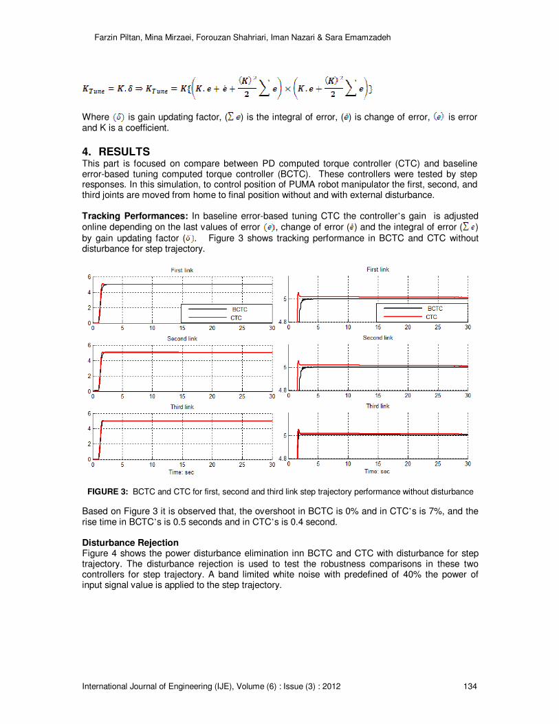
4. RESULTS This part is focused on compare between PD computed torque controller (CTC) and baseline error-based tuning computed torque controller (BCTC). These controllers were tested by step responses. In this simulation, to control position of PUMA robot manipulator the first, second, and third joints are moved from home to final position without and with external disturbance. Tracking Performances: In baseline error-based tuning CTC the controller’s gain is adjusted online depending on the last values of error , change of error ( ) and the integral of error ( )
by gain updating factor ( . Figure 3 shows tracking performance in BCTC and CTC without disturbance for step trajectory.
FIGURE 3: BCTC and CTC for first, second and third link step trajectory performance without disturbance
Based on Figure 3 it is observed that, the overshoot in BCTC is 0% and in CTC’s is 7%, and the rise time in BCTC’s is 0.5 seconds and in CTC’s is 0.4 second. Disturbance Rejection Figure 4 shows the power disturbance elimination inn BCTC and CTC with disturbance for step trajectory. The disturbance rejection is used to test the robustness comparisons in these two controllers for step trajectory. A band limited white noise with predefined of 40% the power of input signal value is applied to the step trajectory.

Farzin Piltan, Mina Mirzaei, Forouzan Shahriari, Iman Nazari & Sara Emamzadeh
International Journal of Engineering (IJE), Volume (6) : Issue (3) : 2012 135
FIGURE 4: BCTC and CTC for first, second and third link trajectory with 40%external disturbance
Based on Figure 4; by comparing step response trajectory with 40% disturbance of relative to the input signal amplitude in BCTC and CTC, BCTC’s overshoot about (0%) is lower than CTC’s (12%). CTC’s rise time (1 seconds) is lower than BCTC’s (1.4 second). Besides the Steady State and RMS error in BCTC and CTC it is observed that, error performances in BCTC (Steady State error =1.3e-5 and RMS error=1.8e-5) are about lower than CTC’s (Steady State error=0.01 and RMS error=0.015). Based on Figure 4, CTC has moderately oscillation in trajectory response with regard to 40% of the input signal amplitude disturbance but BCTC has stability in trajectory responses in presence of uncertainty and external disturbance. Based on Figure 4 in presence of 40% unstructured disturbance, BCTC’s is more robust than CTC because BCTC can auto-tune the coefficient as the dynamic manipulator parameter’s change and in presence of external disturbance whereas CTC cannot. The BCTC gives significant steady state error performance when compared to CTC. When applied 40% disturbances in BCTC the RMS error increased approximately 15.5% (percent of increase the BCTC RMS
error= ) and in CTC the RMS error increased
approximately 125% (percent of increase the PD-SMC RMS
error= ).
5. CONCLUSION In this research, a baseline error-based tuning computed torque controller (BCTC) is design and applied to robot manipulator. Pure CTC has difficulty in handling unstructured model uncertainties. It is possible to solve this problem by combining CTC and baseline error-based tuning. The controller gain is adjusted by baseline error-based tuning method. The gainupdating factor ( ) of baseline error-based tuning part can be changed with the changes in error, change of error and the integral (summation) of error. In pure CTC the controller gain is chosen by trial and error, which means pure CTC had to have a prior knowledge of the system uncertainty. If the knowledge is not available error performance is go up.
REFERENCES [1] T. R. Kurfess, Robotics and automation handbook: CRC, 2005.

Farzin Piltan, Mina Mirzaei, Forouzan Shahriari, Iman Nazari & Sara Emamzadeh
International Journal of Engineering (IJE), Volume (6) : Issue (3) : 2012 136
[2] J. J. E. Slotine and W. Li, Applied nonlinear control vol. 461: Prentice hall Englewood Cliffs, NJ, 1991.
[3] K. Ogata, Modern control engineering: Prentice Hall, 2009. [4] L. Cheng, Z. G. Hou, M. Tan, D. Liu and A. M. Zou, "Multi-agent based adaptive consensus
control for multiple manipulators with kinematic uncertainties," 2008, pp. 189-194. [5] J. J. D'Azzo, C. H. Houpis and S. N. Sheldon, Linear control system analysis and design
with MATLAB: CRC, 2003. [6] B. Siciliano and O. Khatib, Springer handbook of robotics: Springer-Verlag New York Inc,
2008. [7] I. Boiko, L. Fridman, A. Pisano and E. Usai, "Analysis of chattering in systems with second-
order sliding modes," IEEE Transactions on Automatic Control, No. 11, vol. 52,pp. 2085-2102, 2007.
[8] J. Wang, A. Rad and P. Chan, "Indirect adaptive fuzzy sliding mode control: Part I: fuzzy
switching," Fuzzy Sets and Systems, No. 1, vol. 122,pp. 21-30, 2001. [9] C. Wu, "Robot accuracy analysis based on kinematics," IEEE Journal of Robotics and
Automation, No. 3, vol. 2, pp. 171-179, 1986. [10] H. Zhang and R. P. Paul, "A parallel solution to robot inverse kinematics," IEEE conference
proceeding, 2002, pp. 1140-1145. [11] J. Kieffer, "A path following algorithm for manipulator inverse kinematics," IEEE conference
proceeding, 2002, pp. 475-480. [12] Z. Ahmad and A. Guez, "On the solution to the inverse kinematic problem(of robot)," IEEE
conference proceeding, 1990, pp. 1692-1697. [13] F. T. Cheng, T. L. Hour, Y. Y. Sun and T. H. Chen, "Study and resolution of singularities for
a 6-DOF PUMA manipulator," Systems, Man, and Cybernetics, Part B: Cybernetics, IEEE Transactions on, No. 2, vol. 27, pp. 332-343, 2002.
[14] M. W. Spong and M. Vidyasagar, Robot dynamics and control: Wiley-India, 2009. [15] A. Vivas and V. Mosquera, "Predictive functional control of a PUMA robot," Conference
Proceedings, 2005. [16] D. Nguyen-Tuong, M. Seeger and J. Peters, "Computed torque control with nonparametric
regression models," IEEE conference proceeding, 2008, pp. 212-217. [17] V. Utkin, "Variable structure systems with sliding modes," Automatic Control, IEEE
Transactions on, No. 2, vol. 22, pp. 212-222, 2002. [18] R. A. DeCarlo, S. H. Zak and G. P. Matthews, "Variable structure control of nonlinear
multivariable systems: a tutorial," Proceedings of the IEEE, No. 3, vol. 76, pp. 212-232, 2002.
[19] K. D. Young, V. Utkin and U. Ozguner, "A control engineer's guide to sliding mode control,"
IEEE conference proceeding, 2002, pp. 1-14.

Farzin Piltan, Mina Mirzaei, Forouzan Shahriari, Iman Nazari & Sara Emamzadeh
International Journal of Engineering (IJE), Volume (6) : Issue (3) : 2012 137
[20] O. Kaynak, "Guest editorial special section on computationally intelligent methodologies and sliding-mode control," IEEE Transactions on Industrial Electronics, No. 1, vol. 48, pp. 2-3, 2001.
[21] J. J. Slotine and S. Sastry, "Tracking control of non-linear systems using sliding surfaces,
with application to robot manipulators†," International Journal of Control, No. 2, vol. 38, pp. 465-492, 1983.
[22] J. J. E. Slotine, "Sliding controller design for non-linear systems," International Journal of
Control, No. 2, vol. 40, pp. 421-434, 1984. [23] R. Palm, "Sliding mode fuzzy control," IEEE conference proceeding,2002, pp. 519-526. [24] C. C. Weng and W. S. Yu, "Adaptive fuzzy sliding mode control for linear time-varying
uncertain systems," IEEE conference proceeding, 2008, pp. 1483-1490. [25] M. Ertugrul and O. Kaynak, "Neuro sliding mode control of robotic manipulators,"
Mechatronics Journal, No. 1, vol. 10, pp. 239-263, 2000. [26] P. Kachroo and M. Tomizuka, "Chattering reduction and error convergence in the sliding-
mode control of a class of nonlinear systems," Automatic Control, IEEE Transactions on, No. 7, vol. 41, pp. 1063-1068, 2002.
[27] H. Elmali and N. Olgac, "Implementation of sliding mode control with perturbation
estimation (SMCPE)," Control Systems Technology, IEEE Transactions on, No. 1, vol. 4, pp. 79-85, 2002.
[28] J. Moura and N. Olgac, "A comparative study on simulations vs. experiments of SMCPE,"
IEEE conference proceeding, 2002, pp. 996-1000. [29] Y. Li and Q. Xu, "Adaptive Sliding Mode Control With Perturbation Estimation and PID
Sliding Surface for Motion Tracking of a Piezo-Driven Micromanipulator," Control Systems Technology, IEEE Transactions on, No. 4, vol. 18, pp. 798-810, 2010.
[30] B. Wu, Y. Dong, S. Wu, D. Xu and K. Zhao, "An integral variable structure controller with fuzzy tuning design for electro-hydraulic driving Stewart platform," IEEE conference proceeding, 2006, pp. 5-945.
[31] Farzin Piltan , N. Sulaiman, Zahra Tajpaykar, Payman Ferdosali, Mehdi Rashidi, “Design
Artificial Nonlinear Robust Controller Based on CTLC and FSMC with Tunable Gain,” International Journal of Robotic and Automation, 2 (3): 205-220, 2011.
[32] Farzin Piltan, A. R. Salehi and Nasri B Sulaiman.,” Design artificial robust control of second
order system based on adaptive fuzzy gain scheduling,” world applied science journal (WASJ), 13 (5): 1085-1092, 2011
[33] Farzin Piltan, N. Sulaiman, Atefeh Gavahian, Samira Soltani, Samaneh Roosta, “Design
Mathematical Tunable Gain PID-Like Sliding Mode Fuzzy Controller with Minimum Rule Base,” International Journal of Robotic and Automation, 2 (3): 146-156, 2011.
[34] Farzin Piltan , A. Zare, Nasri B. Sulaiman, M. H. Marhaban and R. Ramli, , “A Model Free
Robust Sliding Surface Slope Adjustment in Sliding Mode Control for Robot Manipulator,” World Applied Science Journal, 12 (12): 2330-2336, 2011.
[35] Farzin Piltan , A. H. Aryanfar, Nasri B. Sulaiman, M. H. Marhaban and R. Ramli “Design
Adaptive Fuzzy Robust Controllers for Robot Manipulator,” World Applied Science Journal, 12 (12): 2317-2329, 2011.

Farzin Piltan, Mina Mirzaei, Forouzan Shahriari, Iman Nazari & Sara Emamzadeh
International Journal of Engineering (IJE), Volume (6) : Issue (3) : 2012 138
[36] Farzin Piltan, N. Sulaiman , Arash Zargari, Mohammad Keshavarz, Ali Badri , “Design PID-
Like Fuzzy Controller With Minimum Rule Base and Mathematical Proposed On-line Tunable Gain: Applied to Robot Manipulator,” International Journal of Artificial intelligence and expert system, 2 (4):184-195, 2011.
[37] Farzin Piltan, Nasri Sulaiman, M. H. Marhaban and R. Ramli, “Design On-Line Tunable
Gain Artificial Nonlinear Controller,” Journal of Advances In Computer Research, 2 (4): 75-83, 2011.
[38] Farzin Piltan, N. Sulaiman, Payman Ferdosali, Iraj Assadi Talooki, “ Design Model Free
Fuzzy Sliding Mode Control: Applied to Internal Combustion Engine,” International Journal of Engineering, 5 (4):302-312, 2011.
[39] Farzin Piltan, N. Sulaiman, Samaneh Roosta, M.H. Marhaban, R. Ramli, “Design a New
Sliding Mode Adaptive Hybrid Fuzzy Controller,” Journal of Advanced Science & Engineering Research , 1 (1): 115-123, 2011.
[40] Farzin Piltan, Atefe Gavahian, N. Sulaiman, M.H. Marhaban, R. Ramli, “Novel Sliding Mode
Controller for robot manipulator using FPGA,” Journal of Advanced Science & Engineering Research, 1 (1): 1-22, 2011.
[41] Farzin Piltan, N. Sulaiman, A. Jalali & F. Danesh Narouei, “Design of Model Free Adaptive
Fuzzy Computed Torque Controller: Applied to Nonlinear Second Order System,” International Journal of Robotics and Automation, 2 (4):232-244, 2011.
[42] Farzin Piltan, N. Sulaiman, Iraj Asadi Talooki, Payman Ferdosali, “Control of IC Engine:
Design a Novel MIMO Fuzzy Backstepping Adaptive Based Fuzzy Estimator Variable Structure Control ,” International Journal of Robotics and Automation, 2 (5):360-380, 2011.
[43] Farzin Piltan, N. Sulaiman, Payman Ferdosali, Mehdi Rashidi, Zahra Tajpeikar, “Adaptive
MIMO Fuzzy Compensate Fuzzy Sliding Mode Algorithm: Applied to Second Order Nonlinear System,” International Journal of Engineering, 5 (5): 380-398, 2011.
[44] Farzin Piltan, N. Sulaiman, Hajar Nasiri, Sadeq Allahdadi, Mohammad A. Bairami, “Novel
Robot Manipulator Adaptive Artificial Control: Design a Novel SISO Adaptive Fuzzy Sliding Algorithm Inverse Dynamic Like Method,” International Journal of Engineering, 5 (5): 399-418, 2011.
[45] Farzin Piltan, N. Sulaiman, Sadeq Allahdadi, Mohammadali Dialame, Abbas Zare, “Position
Control of Robot Manipulator: Design a Novel SISO Adaptive Sliding Mode Fuzzy PD Fuzzy Sliding Mode Control,” International Journal of Artificial intelligence and Expert System, 2 (5):208-228, 2011.
[46] Farzin Piltan, SH. Tayebi HAGHIGHI, N. Sulaiman, Iman Nazari, Sobhan Siamak, “Artificial
Control of PUMA Robot Manipulator: A-Review of Fuzzy Inference Engine And Application to Classical Controller ,” International Journal of Robotics and Automation, 2 (5):401-425, 2011.
[47] Farzin Piltan, N. Sulaiman, Abbas Zare, Sadeq Allahdadi, Mohammadali Dialame, “Design
Adaptive Fuzzy Inference Sliding Mode Algorithm: Applied to Robot Arm,” International Journal of Robotics and Automation , 2 (5): 283-297, 2011.
[48] Farzin Piltan, Amin Jalali, N. Sulaiman, Atefeh Gavahian, Sobhan Siamak, “Novel Artificial
Control of Nonlinear Uncertain System: Design a Novel Modified PSO SISO Lyapunov
Farzin Piltan, Mina Mirzaei, Forouzan Shahriari, Iman Nazari & Sara Emamzadeh
International Journal of Engineering (IJE), Volume (6) : Issue (3) : 2012 139
Based Fuzzy Sliding Mode Algorithm ,” International Journal of Robotics and Automation, 2 (5): 298-316, 2011.
[49] Farzin Piltan, N. Sulaiman, Amin Jalali, Koorosh Aslansefat, “Evolutionary Design of
Mathematical tunable FPGA Based MIMO Fuzzy Estimator Sliding Mode Based Lyapunov Algorithm: Applied to Robot Manipulator,” International Journal of Robotics and Automation, 2 (5):317-343, 2011.
[50] Farzin Piltan, N. Sulaiman, Samaneh Roosta, Atefeh Gavahian, Samira Soltani,
“Evolutionary Design of Backstepping Artificial Sliding Mode Based Position Algorithm: Applied to Robot Manipulator,” International Journal of Engineering, 5 (5):419-434, 2011.
[51] Farzin Piltan, N. Sulaiman, S.Soltani, M. H. Marhaban & R. Ramli, “An Adaptive sliding
surface slope adjustment in PD Sliding Mode Fuzzy Control for Robot Manipulator,” International Journal of Control and Automation , 4 (3): 65-76, 2011.
[52] Farzin Piltan, N. Sulaiman, Mehdi Rashidi, Zahra Tajpaikar, Payman Ferdosali, “Design
and Implementation of Sliding Mode Algorithm: Applied to Robot Manipulator-A Review ,” International Journal of Robotics and Automation, 2 (5):265-282, 2011.
[53] Farzin Piltan, N. Sulaiman, Amin Jalali, Sobhan Siamak, and Iman Nazari, “Control of
Robot Manipulator: Design a Novel Tuning MIMO Fuzzy Backstepping Adaptive Based Fuzzy Estimator Variable Structure Control ,” International Journal of Control and Automation, 4 (4):91-110, 2011.
[54] Farzin Piltan, N. Sulaiman, Atefeh Gavahian, Samaneh Roosta, Samira Soltani, “On line
Tuning Premise and Consequence FIS: Design Fuzzy Adaptive Fuzzy Sliding Mode Controller Based on Lyaponuv Theory,” International Journal of Robotics and Automation, 2 (5):381-400, 2011.
[55] Farzin Piltan, N. Sulaiman, Samaneh Roosta, Atefeh Gavahian, Samira Soltani, “Artificial
Chattering Free on-line Fuzzy Sliding Mode Algorithm for Uncertain System: Applied in Robot Manipulator,” International Journal of Engineering, 5 (5):360-379, 2011.
[56] Farzin Piltan, N. Sulaiman and I.AsadiTalooki, “Evolutionary Design on-line Sliding Fuzzy
Gain Scheduling Sliding Mode Algorithm: Applied to Internal Combustion Engine,” International Journal of Engineering Science and Technology, 3 (10):7301-7308, 2011.
[57] Farzin Piltan, Nasri B Sulaiman, Iraj Asadi Talooki and Payman Ferdosali.,” Designing On-
Line Tunable Gain Fuzzy Sliding Mode Controller Using Sliding Mode Fuzzy Algorithm: Applied to Internal Combustion Engine,” world applied science journal (WASJ), 15 (3): 422-428, 2011
[58] B. K. Yoo and W. C. Ham, "Adaptive control of robot manipulator using fuzzy
compensator," Fuzzy Systems, IEEE Transactions on, No. 2, vol. 8, pp. 186-199, 2002. [59] H. Medhaffar, N. Derbel and T. Damak, "A decoupled fuzzy indirect adaptive sliding mode
controller with application to robot manipulator," International Journal of Modelling, Identification and Control, No. 1, vol. 1, pp. 23-29, 2006.
[60] Y. Guo and P. Y. Woo, "An adaptive fuzzy sliding mode controller for robotic manipulators,"
Systems, Man and Cybernetics, Part A: Systems and Humans, IEEE Transactions on, No. 2, vol. 33, pp. 149-159, 2003.
[61] C. M. Lin and C. F. Hsu, "Adaptive fuzzy sliding-mode control for induction servomotor
systems," Energy Conversion, IEEE Transactions on, No. 2, vol. 19, pp. 362-368, 2004.

Farzin Piltan, Mina Mirzaei, Forouzan Shahriari, Iman Nazari & Sara Emamzadeh
International Journal of Engineering (IJE), Volume (6) : Issue (3) : 2012 140
[62] Xiaosong. Lu, "An investigation of adaptive fuzzy sliding mode control for robot
manipulator," Carleton university Ottawa,2007. [63] S. Lentijo, S. Pytel, A. Monti, J. Hudgins, E. Santi and G. Simin, "FPGA based sliding mode
control for high frequency power converters," IEEE Conference, 2004, pp. 3588-3592. [64] B. S. R. Armstrong, "Dynamics for robot control: friction modeling and ensuring excitation
during parameter identification," 1988. [65] C. L. Clover, "Control system design for robots used in simulating dynamic force and
moment interaction in virtual reality applications," 1996. [66] K. R. Horspool, Cartesian-space Adaptive Control for Dual-arm Force Control Using
Industrial Robots: University of New Mexico, 2003. [67] B. Armstrong, O. Khatib and J. Burdick, "The explicit dynamic model and inertial
parameters of the PUMA 560 arm," IEEE Conference, 2002, pp. 510-518. [68] P. I. Corke and B. Armstrong-Helouvry, "A search for consensus among model parameters
reported for the PUMA 560 robot," IEEE Conference, 2002, pp. 1608-1613. [69] Farzin Piltan, N. Sulaiman, M. H. Marhaban, Adel Nowzary, Mostafa Tohidian,” “Design of
FPGA based sliding mode controller for robot manipulator,” International Journal of Robotic and Automation, 2 (3): 183-204, 2011.
[70] I. Eksin, M. Guzelkaya and S. Tokat, "Sliding surface slope adjustment in fuzzy sliding
mode controller," Mediterranean Conference, 2002, pp. 160-168. [71] Farzin Piltan, H. Rezaie, B. Boroomand, Arman Jahed,” Design robust back stepping
online tuning feedback linearization control applied to IC engine,” International Journal of Advance Science and Technology, 42: 183-204, 2012.
[72] Farzin Piltan, I. Nazari, S. Siamak, P. Ferdosali ,”Methodology of FPGA-based
mathematical error-based tuning sliding mode controller” International Journal of Control and Automation, 5(1): 89-110, 2012.
[73] Farzin Piltan, M. A. Dialame, A. Zare, A. Badri ,”Design Novel Lookup table changed Auto
Tuning FSMC: Applied to Robot Manipulator” International Journal of Engineering, 6(1): 25-40, 2012.
[74] Farzin Piltan, B. Boroomand, A. Jahed, H. Rezaie ,”Methodology of Mathematical Error-
Based Tuning Sliding Mode Controller” International Journal of Engineering, 6(2): 96-112, 2012.
[75] Farzin Piltan, F. Aghayari, M. R. Rashidian, M. Shamsodini, ”A New Estimate Sliding Mode
Fuzzy Controller for Robotic Manipulator” International Journal of Robotics and Automation, 3(1): 45-58, 2012.
[76] Farzin Piltan, M. Keshavarz, A. Badri, A. Zargari , ”Design novel nonlinear controller
applied to robot manipulator: design new feedback linearization fuzzy controller with minimum rule base tuning method” International Journal of Robotics and Automation, 3(1): 1-18, 2012.
[77] Piltan, F., et al. "Design sliding mode controller for robot manipulator with artificial tunable
gain". Canaidian Journal of pure and applied science, 5 (2), 1573-1579, 2011.

Farzin Piltan, Mina Mirzaei, Forouzan Shahriari, Iman Nazari & Sara Emamzadeh
International Journal of Engineering (IJE), Volume (6) : Issue (3) : 2012 141
[78] Farzin Piltan, A. Hosainpour, E. Mazlomian, M.Shamsodini, M.H Yarmahmoudi. ”Online
Tuning Chattering Free Sliding Mode Fuzzy Control Design: Lyapunov Approach” International Journal of Robotics and Automation, 3(3): 2012.
[79] Farzin Piltan , M.H. Yarmahmoudi, M. Shamsodini, E.Mazlomian, A.Hosainpour. ” PUMA-
560 Robot Manipulator Position Computed Torque Control Methods Using MATLAB/SIMULINK and Their Integration into Graduate Nonlinear Control and MATLAB Courses” International Journal of Robotics and Automation, 3(3): 2012.
[80] Farzin Piltan, R. Bayat, F. Aghayari, B. Boroomand. “Design Error-Based Linear Model-
Free Evaluation Performance Computed Torque Controller” International Journal of Robotics and Automation, 3(3): 2012.
[81] Farzin Piltan, S. Emamzadeh, Z. Hivand, F. Shahriyari & Mina Mirazaei . ” PUMA-560 Robot
Manipulator Position Sliding Mode Control Methods Using MATLAB/SIMULINK and Their Integration into Graduate/Undergraduate Nonlinear Control, Robotics and MATLAB Courses” International Journal of Robotics and Automation, 3(3): 2012.
[82] Farzin Piltan, J. Meigolinedjad, S. Mehrara, S. Rahmdel. ” Evaluation Performance of 2
nd
Order Nonlinear System: Baseline Control Tunable Gain Sliding Mode Methodology” International Journal of Robotics and Automation, 3(3): 2012.
[83] Farzin Piltan, S. Rahmdel, S. Mehrara, R. Bayat.” Sliding Mode Methodology Vs. Computed
Torque Methodology Using MATLAB/SIMULINK and Their Integration into Graduate Nonlinear Control Courses” International Journal of Engineering, 3(3): 2012.

Farzin Piltan, Sajad Rahmdel, Saleh Mehrara & Reza Bayat
International Journal of Engineering (IJE), Volume (6) : Issue (3) : 2012 142
Sliding Mode Methodology Vs. Computed Torque Methodology Using MATLAB/SIMULINK and Their
Integration into Graduate Nonlinear Control Courses
Farzin Piltan [email protected] Industrial Electrical and Electronic Engineering SanatkadeheSabze Pasargad. CO (S.S.P. Co), NO:16 , PO.Code 71347-66773, Fourth floor Dena Apr , Seven Tir Ave , Shiraz , Iran
Sajad Rahmdel [email protected] Industrial Electrical and Electronic Engineering SanatkadeheSabze Pasargad. CO (S.S.P. Co), NO:16 ,PO.Code 71347-66773, Fourth floor Dena Apr , Seven Tir Ave , Shiraz , Iran
Saleh Mehrara [email protected] Industrial Electrical and Electronic Engineering SanatkadeheSabze Pasargad. CO (S.S.P. Co), NO:16 ,PO.Code 71347-66773, Fourth floor Dena Apr , Seven Tir Ave , Shiraz , Iran
Reza Bayat [email protected] Industrial Electrical and Electronic Engineering SanatkadeheSabze Pasargad. CO (S.S.P. Co), NO:16 ,PO.Code 71347-66773, Fourth floor Dena Apr , Seven Tir Ave , Shiraz , Iran
Abstract
Design a nonlinear controller for second order nonlinear uncertain dynamical systems is one of the most important challenging works. This paper focuses on the design, implementation and analysis of a chattering free sliding mode controller for highly nonlinear dynamic PUMA robot manipulator and compare to computed torque controller, in presence of uncertainties. In order to provide high performance nonlinear methodology, sliding mode controller and computed torque controller are selected. Pure sliding mode controller and computed torque controller can be used to control of partly known nonlinear dynamic parameters of robot manipulator. Conversely, pure sliding mode controller is used in many applications; it has an important drawback namely; chattering phenomenon which it can causes some problems such as saturation and heat the mechanical parts of robot manipulators or drivers. In order to reduce the chattering this research is used the linear saturation function boundary layer method instead of switching function method in pure sliding mode controller. These simulation models are developed as a part of a software laboratory to support and enhance graduate/undergraduate robotics courses, nonlinear control courses and MATLAB/SIMULINK courses at research and development company (SSP Co.) research center, Shiraz, Iran.
Keywords: MATLAB/SIMULINK, PUMA 560 Robot Manipulator, Nonlinear Position Control Method, Sliding Mode Control, Computed Torque Control, Chattering Free, and Nonlinear Control.

Farzin Piltan, Sajad Rahmdel, Saleh Mehrara & Reza Bayat
International Journal of Engineering (IJE), Volume (6) : Issue (3) : 2012 143
1. INTRODUCTION Computer modeling, simulation and implementation tools have been widely used to support and develop nonlinear control, robotics, and MATLAB/SIMULINK courses. MATLAB with its toolboxes such as SIMULINK [1] is one of the most accepted software packages used by researchers to enhance teaching the transient and steady-state characteristics of control and robotic courses [3_7]. In an effort to modeling and implement robotics, nonlinear control and advanced MATLAB/SIMULINK courses at research and development SSP Co., authors have developed MATLAB/SIMULINK models for learn the basic information in field of nonlinear control and industrial robot manipulator [8, 9].
Controller is a device which can sense information from linear or nonlinear system (e.g., robot manipulator) to improve the systems performance [3]. The main targets in designing control systems are stability, good disturbance rejection, and small tracking error[5]. Several industrial robot manipulators are controlled by linear methodologies (e.g., Proportional-Derivative (PD) controller, Proportional- Integral (PI) controller or Proportional- Integral-Derivative (PID) controller), but when robot manipulator works with various payloads and have uncertainty in dynamic models this technique has limitations. From the control point of view, uncertainty is divided into two main groups: uncertainty in unstructured inputs (e.g., noise, disturbance) and uncertainty in structure dynamics (e.g., payload, parameter variations). In some applications robot manipulators are used in an unknown and unstructured environment, therefore strong mathematical tools used in new control methodologies to design nonlinear robust controller with an acceptable performance (e.g., minimum error, good trajectory, disturbance rejection [10-18]. Sliding mode controller is a powerful nonlinear robust controller under condition of partly uncertain dynamic parameters of system [7]. This controller is used to control of highly nonlinear systems especially for robot manipulators. Chattering phenomenon and nonlinear equivalent dynamic formulation in uncertain dynamic parameter are two main drawbacks in pure sliding mode controller [20]. The main reason to opt for this controller is its acceptable control performance in wide range and solves two most important challenging topics in control which names, stability and robustness [7, 17-20]. Sliding mode controller is divided into two main sub controllers: discontinues controller and equivalent controller . Discontinues controller
causes an acceptable tracking performance at the expense of very fast switching. Conversely in this theory good trajectory following is based on fast switching, fast switching is caused to have system instability and chattering phenomenon. Fine tuning the sliding surface slope is based on nonlinear equivalent part [1, 6]. However, this controller is used in many applications but, pure sliding mode controller has two most important challenges: chattering phenomenon and nonlinear equivalent dynamic formulation in uncertain parameters[20]. Chattering phenomenon (Figure 1) can causes some problems such as saturation and heat the mechanical parts of robot manipulators or drivers. To reduce or eliminate the chattering, various papers have been reported by many researchers which classified into two most important methods: boundary layer saturation method and estimated uncertainties method [1]. In boundary layer saturation method, the basic idea is the discontinuous method replacement by saturation (linear) method with small neighborhood of the switching surface. This replacement caused to increase the error performance against with the considerable chattering reduction. Slotine and Sastry have introduced boundary layer method instead of discontinuous method to reduce the chattering[21]. Slotine has presented sliding mode with boundary layer to improve the industry application [22]. Palm has presented a fuzzy method to nonlinear approximation instead of linear approximation inside the boundary layer to improve the chattering and control the result performance[23]. Moreover, Weng and Yu improved the previous method by using a new method in fuzzy nonlinear approximation inside the boundary layer and adaptive method[24]. As mentioned [24]sliding mode fuzzy controller (SMFC) is fuzzy controller based on sliding mode technique to most exceptional stability and robustness. Sliding mode fuzzy controller has the two most important advantages: reduce the number of fuzzy rule base and increase robustness and stability.

Farzin Piltan, Sajad Rahmdel, Saleh Mehrara & Reza Bayat
International Journal of Engineering (IJE), Volume (6) : Issue (3) : 2012 144
Conversely sliding mode fuzzy controller has the above advantages, define the sliding surface slope coefficient very carefully is the main disadvantage of this controller. Estimated uncertainty method used in term of uncertainty estimator to compensation of the system uncertainties. It has been used to solve the chattering phenomenon and also nonlinear equivalent dynamic. If estimator has an acceptable performance to compensate the uncertainties, the chattering is reduced. Research on estimated uncertainty to reduce the chattering is significantly growing as their applications such as industrial automation and robot manipulator. For instance, the applications of artificial intelligence, neural networks and fuzzy logic on estimated uncertainty method have been reported in [25-28]. Wu et al. [30] have proposed a simple fuzzy estimator controller beside the discontinuous and equivalent control terms to reduce the chattering. Their design had three main parts i.e. equivalent, discontinuous and fuzzy estimator tuning part which has reduced the chattering very well. Elmali et al. [27]and Li and Xu [29] have addressed sliding mode control with perturbation estimation method (SMCPE) to reduce the classical sliding mode chattering. This method was tested for the tracking control of the first two links of a SCARA type HITACHI robot. In this technique, digital controller is used to increase the system’s response quality. However this controller’s response is very fast and robust but it has chattering phenomenon. Design a robust controller for robot manipulator is essential because robot manipulator has highly nonlinear dynamic parameters. Computed torque controller (CTC) is a powerful nonlinear controller which it widely used in control of robot manipulator. It is based on feedback linearization and computes the required arm torques using the nonlinear feedback control law. This controller works very well when all dynamic and physical parameters are known but when the robot manipulator has variation in dynamic parameters, in this situation the controller has no acceptable performance[14]. In practice, most of physical systems (e.g., robot manipulators) parameters are unknown or time variant, therefore, computed torque like controller used to compensate dynamic equation of robot manipulator[1, 6]. Research on computed torque controller is significantly growing on robot manipulator application which has been reported in [1, 6, 15-16]. Vivas and Mosquera [15]have proposed a predictive functional controller and compare to computed torque controller for tracking response in uncertain environment. However both controllers have been used in feedback linearization, but predictive strategy gives better result as a performance. A computed torque control with non parametric regression models have been presented for a robot arm[16]. This controller also has been problem in uncertain dynamic models. Based on [1, 6]and [15-16] computed torque controller is a significant nonlinear controller to certain systems which it is based on feedback linearization and computes the required arm torques using the nonlinear feedback control law. This paper is organized as follows: In section 2, dynamic formulation of robot manipulator is presented. Detail of classical SMC and MATLAB/SIMULINK implementation of this controller is presented in section 3. Detail of classical CTC and MATLAB/SIMULINK implementation of this controller is presented in section 4. In section 5, the simulation result is presented and finally in section 6, the conclusion is presented.
2. PUMA 560 ROBOT MANIPULATOR DYNAMIC FORMULATION Dynamics of PUMA560 Robot Manipulator To position control of robot manipulator, the second three axes are locked the dynamic equation of PUMA robot manipulator is given by [77-80];
(1)
Where

Farzin Piltan, Sajad Rahmdel, Saleh Mehrara & Reza Bayat
International Journal of Engineering (IJE), Volume (6) : Issue (3) : 2012 145
(2)
is computed as
o3
(4)
(5)
(6)
(7)
(8)
(9)
(10)
(11)
(12)
(13)
and Corilios ( ) matrix is calculated as the following
(14)
Where,

Farzin Piltan, Sajad Rahmdel, Saleh Mehrara & Reza Bayat
International Journal of Engineering (IJE), Volume (6) : Issue (3) : 2012 146
(15)
(16)
(17)
(18)
(19)
(20)
(21)
(22)
(23)
(24)
(25)
(26)
consequently coriolis matrix is shown as bellows;
(27)
Moreover Centrifugal ( ) matrix is demonstrated as
(28)
Where,

Farzin Piltan, Sajad Rahmdel, Saleh Mehrara & Reza Bayat
International Journal of Engineering (IJE), Volume (6) : Issue (3) : 2012 147
(29)
(30)
(31)
(32)
(33)
(34)
(35)
(36)
In this research , as a result
(37)
Gravity ( ) Matrix can be written as
(38)
Where,
(39)
(40)
(41)
Suppose is written as follows

Farzin Piltan, Sajad Rahmdel, Saleh Mehrara & Reza Bayat
International Journal of Engineering (IJE), Volume (6) : Issue (3) : 2012 148
(42)
and is introduced as (43)
can be written as (44)
Therefore for PUMA robot manipulator is calculated by the following equations
(45)
(46)
(47)
(48)
(49)
(50)
An information about inertial constant and gravitational constant are shown in Tables 1 and 2 based on the studies carried out by Armstrong [80] and Corke and Armstrong [81].
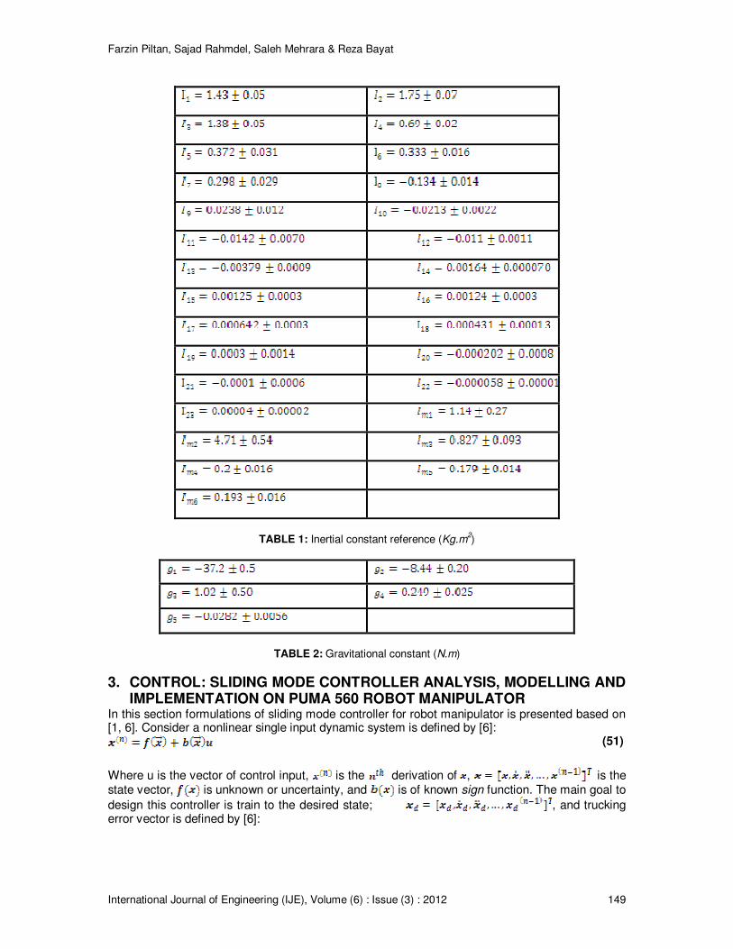
Farzin Piltan, Sajad Rahmdel, Saleh Mehrara & Reza Bayat
International Journal of Engineering (IJE), Volume (6) : Issue (3) : 2012 149
TABLE 1: Inertial constant reference (Kg.m
2)
TABLE 2: Gravitational constant (N.m)
3. CONTROL: SLIDING MODE CONTROLLER ANALYSIS, MODELLING AND IMPLEMENTATION ON PUMA 560 ROBOT MANIPULATOR
In this section formulations of sliding mode controller for robot manipulator is presented based on [1, 6]. Consider a nonlinear single input dynamic system is defined by [6]:
(51)
Where u is the vector of control input, is the derivation of , is the state vector, is unknown or uncertainty, and is of known sign function. The main goal to
design this controller is train to the desired state; , and trucking error vector is defined by [6]:

Farzin Piltan, Sajad Rahmdel, Saleh Mehrara & Reza Bayat
International Journal of Engineering (IJE), Volume (6) : Issue (3) : 2012 150
(52)
A time-varying sliding surface in the state space is given by [6]:
(53)
where λ is the positive constant. To further penalize tracking error, integral part can be used in sliding surface part as follows [6]:
(54)
The main target in this methodology is kept the sliding surface slope near to the zero. Therefore, one of the common strategies is to find input outside of [6].
(55)
where ζ is positive constant.
If S(0)>0 (56)
To eliminate the derivative term, it is used an integral term from t=0 to t=
(57)
Where is the time that trajectories reach to the sliding surface so, suppose S( defined as
(58)
and
(59)
Equation (81) guarantees time to reach the sliding surface is smaller than since the
trajectories are outside of .
(60)
suppose S is defined as
(61)
The derivation of S, namely, can be calculated as the following;
(62)
suppose the second order system is defined as;
(63)
Where is the dynamic uncertain, and also since , to have the best approximation , is defined as
(64)
A simple solution to get the sliding condition when the dynamic parameters have uncertainty is the switching control law:
(65)
where the switching function is defined as [1, 6]
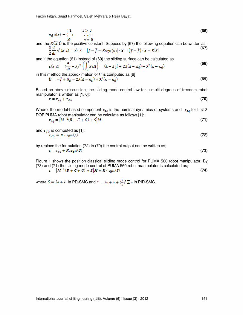
Farzin Piltan, Sajad Rahmdel, Saleh Mehrara & Reza Bayat
International Journal of Engineering (IJE), Volume (6) : Issue (3) : 2012 151
(66)
and the is the positive constant. Suppose by (67) the following equation can be written as,
(67)
and if the equation (61) instead of (60) the sliding surface can be calculated as
(68)
in this method the approximation of is computed as [6]
(69)
Based on above discussion, the sliding mode control law for a multi degrees of freedom robot manipulator is written as [1, 6]:
(70)
Where, the model-based component is the nominal dynamics of systems and for first 3
DOF PUMA robot manipulator can be calculate as follows [1]:
(71)
and is computed as [1];
(72)
by replace the formulation (72) in (70) the control output can be written as;
(73)
Figure 1 shows the position classical sliding mode control for PUMA 560 robot manipulator. By (73) and (71) the sliding mode control of PUMA 560 robot manipulator is calculated as;
(74)
where in PD-SMC and in PID-SMC.
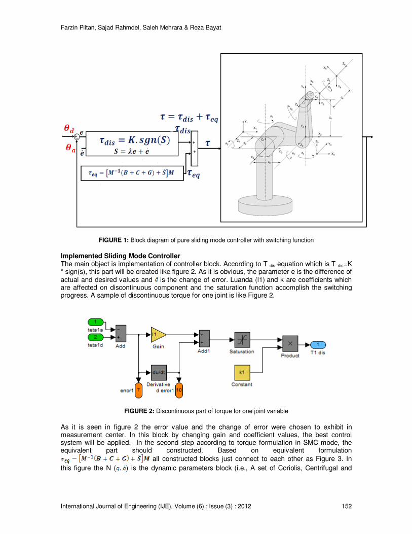
Farzin Piltan, Sajad Rahmdel, Saleh Mehrara & Reza Bayat
International Journal of Engineering (IJE), Volume (6) : Issue (3) : 2012 152
FIGURE 1: Block diagram of pure sliding mode controller with switching function
Implemented Sliding Mode Controller The main object is implementation of controller block. According to T dis equation which is T dis=K * sign(s), this part will be created like figure 2. As it is obvious, the parameter e is the difference of actual and desired values and is the change of error. Luanda (l1) and k are coefficients which are affected on discontinuous component and the saturation function accomplish the switching progress. A sample of discontinuous torque for one joint is like Figure 2.
FIGURE 2: Discontinuous part of torque for one joint variable
As it is seen in figure 2 the error value and the change of error were chosen to exhibit in measurement center. In this block by changing gain and coefficient values, the best control system will be applied. In the second step according to torque formulation in SMC mode, the equivalent part should constructed. Based on equivalent formulation
all constructed blocks just connect to each other as Figure 3. In
this figure the N ( ) is the dynamic parameters block (i.e., A set of Coriolis, Centrifugal and

Farzin Piltan, Sajad Rahmdel, Saleh Mehrara & Reza Bayat
International Journal of Engineering (IJE), Volume (6) : Issue (3) : 2012 153
Gravity blocks) and the derivative of S is apparent. Just by multiplication and summation, the output which is equivalent torque will be obtained.
FIGURE 3: The equivalent part of torque with required blocks
The inputs are thetas and the final outputs are equivalent torque values. The relations between other blocks are just multiplication and summation as mentioned in torque equation. The next phase is calculation of the summation of equivalent part and discontinuous part which make the total torque value. This procedure is depicted in Figure 4.

Farzin Piltan, Sajad Rahmdel, Saleh Mehrara & Reza Bayat
International Journal of Engineering (IJE), Volume (6) : Issue (3) : 2012 154
FIGURE 4: The total value of torque which is summation of equivalent & discontinuous blocks
In the next step transform our subsystems into a general system to form controller block and the outputs will be connected to the plant, in order to execute controlling process. Then, trigger the main inputs with power supply to check validity and performance. In Figure 5 Dynamics, Kinematics, Controller and the measurement center blocks are shown.

Farzin Piltan, Sajad Rahmdel, Saleh Mehrara & Reza Bayat
International Journal of Engineering (IJE), Volume (6) : Issue (3) : 2012 155
FIGURE 5: Measurement center, Controller, Dynamics and Kinematics Blocks
4. CONTROL: COMPUTED TORQUE CONTROLLER ANALYSIS, MODELLING AND IMPLEMENTATION ON PUMA 560 ROBOT MANIPULATOR
Computed torque controller (CTC) is a powerful nonlinear controller which it widely used in control of robot manipulator. It is based on feedback linearization and computes the required arm torques using the nonlinear feedback control law. This controller works very well when all dynamic and physical parameters are known but when the robot manipulator has variation in dynamic parameters, in this situation the controller has no acceptable performance[14]. In practice, most of physical systems (e.g., robot manipulators) parameters are unknown or time variant, therefore, computed torque like controller used to compensate dynamic equation of robot manipulator[1, 6]. Research on computed torque controller is significantly growing on robot manipulator application which has been reported in [1, 6, 15-16]. Vivas and Mosquera [15]have proposed a predictive functional controller and compare to computed torque controller for tracking response in uncertain environment. However both controllers have been used in feedback linearization, but predictive strategy gives better result as a performance. A computed torque control with non parametric regression models have been presented for a robot arm[16]. This controller also has been problem in uncertain dynamic models. Based on [1, 6]and [15-16] computed torque controller is a significant nonlinear controller to certain systems which it is based on feedback linearization and computes the required arm torques using the nonlinear feedback control law. When all dynamic and physical parameters are known, computed torque controller works fantastically; practically a large amount of systems have uncertainties, therefore sliding mode controller is one of the best case to solve this challenge. The central idea of Computed torque controller (CTC) is feedback linearization so, originally this algorithm is called feedback linearization controller. It has assumed that the desired motion

Farzin Piltan, Sajad Rahmdel, Saleh Mehrara & Reza Bayat
International Journal of Engineering (IJE), Volume (6) : Issue (3) : 2012 156
trajectory for the manipulator , as determined, by a path planner. Defines the tracking error as:
(75)
Where e(t) is error of the plant, is desired input variable, that in our system is desired displacement, is actual displacement. If an alternative linear state-space equation in the form can be defined as
(76)
With and this is known as the Brunousky canonical form. By equation (76) and (77) the Brunousky canonical form can be written in terms of the state
as [1]:
(77)
With
(78)
Then compute the required arm torques using inverse of equation (79), is;
(79)
This is a nonlinear feedback control law that guarantees tracking of desired trajectory. Selecting proportional-plus-derivative (PD) feedback for U(t) results in the PD-computed torque controller [6];
(80)
and the resulting linear error dynamics are
(81)
According to the linear system theory, convergence of the tracking error to zero is guaranteed [6]. Where and are the controller gains. The result schemes is shown in Figure 6, in which two
feedback loops, namely, inner loop and outer loop, which an inner loop is a compensate loop and an outer loop is a tracking error loop.

Farzin Piltan, Sajad Rahmdel, Saleh Mehrara & Reza Bayat
International Journal of Engineering (IJE), Volume (6) : Issue (3) : 2012 157
FIGURE 6: Block diagram of PD-computed torque controller (PD-CTC)
The application of proportional-plus-derivative (PD) computed torque controller to control of PUMA 560 robot manipulator introduced in this part. Suppose that in (82) the nonlinearity term defined by the following term
(82)
Therefore the equation of PD-CTC for control of PUMA 560 robot manipulator is written as the equation of (83);
(83)
The controller based on a formulation (83) is related to robot dynamics therefore it has problems in uncertain conditions.
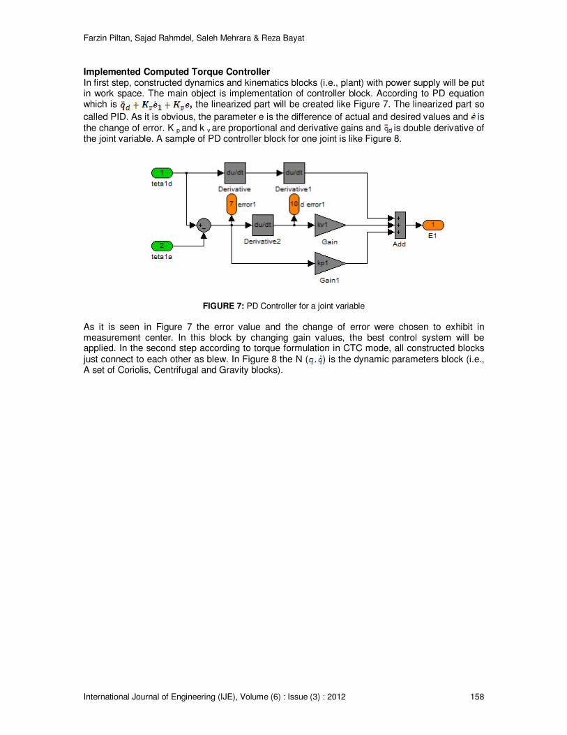
Farzin Piltan, Sajad Rahmdel, Saleh Mehrara & Reza Bayat
International Journal of Engineering (IJE), Volume (6) : Issue (3) : 2012 158
Implemented Computed Torque Controller In first step, constructed dynamics and kinematics blocks (i.e., plant) with power supply will be put in work space. The main object is implementation of controller block. According to PD equation which is , the linearized part will be created like Figure 7. The linearized part so
called PID. As it is obvious, the parameter e is the difference of actual and desired values and is the change of error. K p and k v are proportional and derivative gains and d is double derivative of the joint variable. A sample of PD controller block for one joint is like Figure 8.
FIGURE 7: PD Controller for a joint variable
As it is seen in Figure 7 the error value and the change of error were chosen to exhibit in measurement center. In this block by changing gain values, the best control system will be applied. In the second step according to torque formulation in CTC mode, all constructed blocks just connect to each other as blew. In Figure 8 the N ( ) is the dynamic parameters block (i.e., A set of Coriolis, Centrifugal and Gravity blocks).
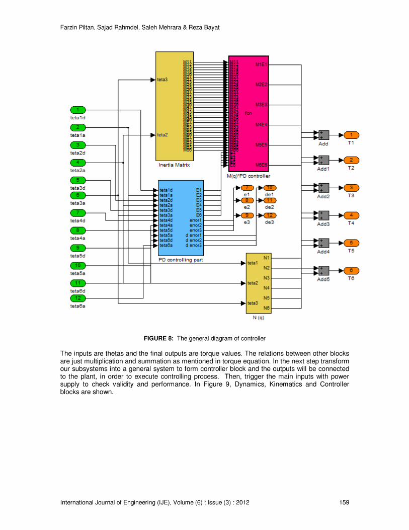
Farzin Piltan, Sajad Rahmdel, Saleh Mehrara & Reza Bayat
International Journal of Engineering (IJE), Volume (6) : Issue (3) : 2012 159
FIGURE 8: The general diagram of controller
The inputs are thetas and the final outputs are torque values. The relations between other blocks are just multiplication and summation as mentioned in torque equation. In the next step transform our subsystems into a general system to form controller block and the outputs will be connected to the plant, in order to execute controlling process. Then, trigger the main inputs with power supply to check validity and performance. In Figure 9, Dynamics, Kinematics and Controller blocks are shown.

Farzin Piltan, Sajad Rahmdel, Saleh Mehrara & Reza Bayat
International Journal of Engineering (IJE), Volume (6) : Issue (3) : 2012 160
FIGURE 9: Controller, Dynamics and Kinematics Blocks
5. RESULTS Sliding mode controller (SMC) and computed torque controller (CTC) were tested to Step responses. In this simulation the first, second, and third joints are moved from home to final position without and with external disturbance. The simulation was implemented in MATLAB/SIMULINK environment. It is noted that, these systems are tested by band limited white noise with a predefined 40% of relative to the input signal amplitude which the sample time is equal to 0.1. This type of noise is used to external disturbance in continuous and hybrid systems. Tracking Performances based on (90) in computed torque controller; the performance of this controller is depended on the PD ( ) coefficients. These coefficients are and computed by trial
and error. Table 3 shows the different coefficient gain in computed torque controller.
1Pk
1Vk 2pk
2Vk 3pk
3Vk RMs error
SS
error1
SS
error2
SS error3
1 8 4 8 4 8 4 2.276e-5 -3.81e-5 -3.81e-5 -3.81e-5
2 30 4 30 4 30 4 1.34e-5 -3.6e-5 -2.54e-5 -1.6e-5
3 1 4 1 4 1 4 0.0039 0.0065 0.0065 0.0065
4 8 40 8 40 8 40 0.502 5.043 5.043 5.043
5 8 0.5 8 0.5 8 0.5 0.0026 0.0043 0.0043 0.0043
TABLE 3: Tuning parameters of a step PD-CTC

Farzin Piltan, Sajad Rahmdel, Saleh Mehrara & Reza Bayat
International Journal of Engineering (IJE), Volume (6) : Issue (3) : 2012 161
Based on this table, the different PD coefficient gain has the different errors therefore minimum error played important role to select the .
Based on (80) in sliding mode controller with switching function; the performance is depended on the gain updating factor ( ) and sliding surface slope coefficient ( ). These two coefficients are computed by trial and error based on Table 4.
1
λ
1k
2λ
2k 3
λ
3
k SS
error1
SS
error2
SS
error3
RMS error
data1
3 30 6 30 6 30 0.1e-3 0.1e-3 -5.3e-15
0.1e-4
data2
30
30 60 30 60
30 -5.17 14.27 -1.142 0.05
data3
3 300
6 300
6 300
2.28 0.97 0.076 0.08
TABLE 4: Tuning parameters of Step SMC with switching function
Based on Table 4, in this research for step inputs and for ramp inputs Based on (84) in sliding mode controller with saturation function (boundary layer); the performance is depended on the gain updating factor ( ), sliding surface slope coefficient ( ) and boundary layer saturation coefficient ( ). These three coefficients are computed by trial and error based on Tables 5.
1
k 1
λ 1
φ 2
k
2
λ 2
φ 3k
3λ
3
φ SS
error1
SS
error2
SS
error3
RMS error
data1
10 1 0.1 10 6 0.1 10 8 0.1 1e-6 1e-6 1e-6 1.2e-6
data2
100
1 0.1 100
6 0.1 100
8 0.1 0.2 0.05 -0.02 -0.037
data3
10 10 0.1 10 60 0.1 10 80 0.1 0.22 -0.21 -0.19 0.09
TABLE 5: Tuning parameters of a step SMC with boundary layer
In this research based on Table 5, for step inputs:
and for ramp inputs: . Figure 10 and 4.2 is shown tracking
performance for CTC, SMC with switching function and SMC with boundary layer without disturbance for step trajectorie. Based on Figure 10; by comparing step response trajectory without disturbance in CTC, SMC with switching function and SMC with boundary layer, SMC with saturation function’s overshoot about (0.94%) is lower than SMC with switching function’s and CTC’s (6.44%). SMC with switching function’s and CTC’s rise time (0.403) is lower than SMC with saturation function’s (0.483). Based on simulation results the Steady State and RMS error in SMC with boundary layer (Steady State error =1e-6 and RMS error=1.2e-6) are fairly lower than CTC’s (Steady State error and RMS error= ) and SMC with switching function’s (Steady State error and RMS error=0.00652). Based on Figure 10 and chattering phenomenon challenge in pure sliding mode controller with switching function, it is found fairly fluctuations in trajectory responses.
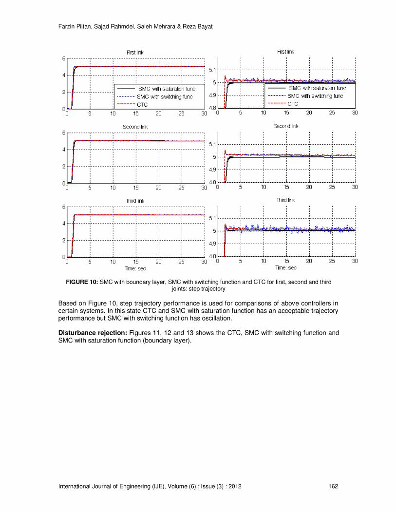
Farzin Piltan, Sajad Rahmdel, Saleh Mehrara & Reza Bayat
International Journal of Engineering (IJE), Volume (6) : Issue (3) : 2012 162
FIGURE 10: SMC with boundary layer, SMC with switching function and CTC for first, second and third joints: step trajectory
Based on Figure 10, step trajectory performance is used for comparisons of above controllers in certain systems. In this state CTC and SMC with saturation function has an acceptable trajectory performance but SMC with switching function has oscillation. Disturbance rejection: Figures 11, 12 and 13 shows the CTC, SMC with switching function and SMC with saturation function (boundary layer).
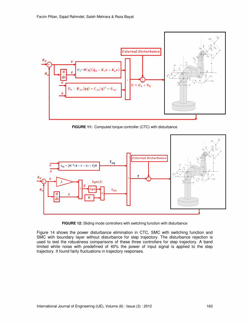
Farzin Piltan, Sajad Rahmdel, Saleh Mehrara & Reza Bayat
International Journal of Engineering (IJE), Volume (6) : Issue (3) : 2012 163
FIGURE 11: Computed torque controller (CTC) with disturbance
FIGURE 12: Sliding mode controllers with switching function with disturbance
Figure 14 shows the power disturbance elimination in CTC, SMC with switching function and SMC with boundary layer without disturbance for step trajectory. The disturbance rejection is used to test the robustness comparisons of these three controllers for step trajectory. A band limited white noise with predefined of 40% the power of input signal is applied to the step trajectory. It found fairly fluctuations in trajectory responses.
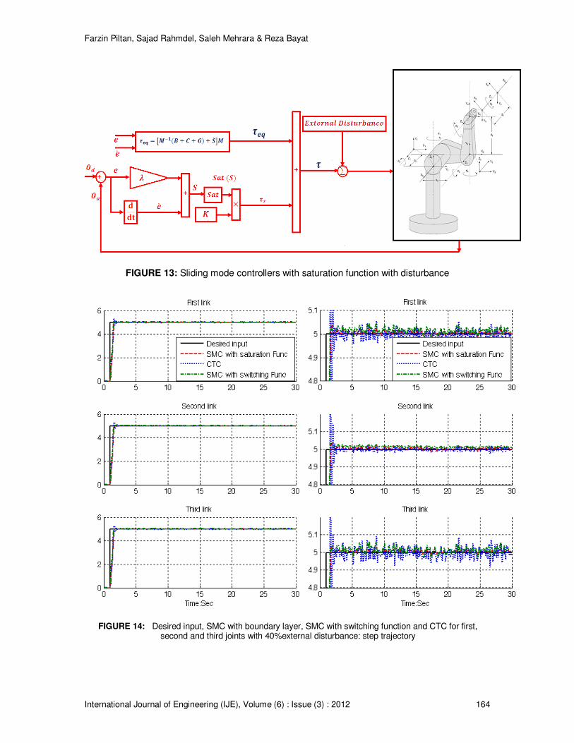
Farzin Piltan, Sajad Rahmdel, Saleh Mehrara & Reza Bayat
International Journal of Engineering (IJE), Volume (6) : Issue (3) : 2012 164
FIGURE 13: Sliding mode controllers with saturation function with disturbance
FIGURE 14: Desired input, SMC with boundary layer, SMC with switching function and CTC for first, second and third joints with 40%external disturbance: step trajectory

Farzin Piltan, Sajad Rahmdel, Saleh Mehrara & Reza Bayat
International Journal of Engineering (IJE), Volume (6) : Issue (3) : 2012 165
Based on Figure 14; by comparing step response trajectory with 40% disturbance of relative to the input signal amplitude in CTC, boundary layer (saturation) SMC and switching mode SMC, SMC with saturation function’s overshoot about (6%) is lower than SMC with switching function’s (13%)and CTC’s (14.8%). SMC with switching function’s and CTC’s rise time (0.5) is lower than SMC with saturation function’s (0.53). Besides the Steady State and RMS error in SMC with boundary layer (Steady State error =10e-4 and RMS error=11e-4) are fairly lower than CTC’s (Steady State error and RMS error= ) and SMC with switching function’s (Steady State error and RMS error=0.98). Based on Figure 14, all three controllers have oscillation in trajectory response with regard to 40% of the input signal amplitude disturbance. All these three controllers have fairly large oscillation with regard to the external disturbance. Based on Figure 14, a step trajectory performance is used for comparisons of above controllers in presence of uncertainties with 40% of input signal amplitude. In this state however boundary layer SMC has relatively moderate oscillations but it is more robust than CTC and SMC with switching function. From the disturbance rejection for boundary layer SMC, SMC with switching function and CTC in presence of disturbance, it was seen that however boundary layer SMC performance is better than SMC with switching function and CTC but it has a limitation against to highly external disturbance. Steady State and RMS Error Figures 15and 16 show the error performance without disturbance and in presence of disturbance in CTC, SMC with switching function and SMC with boundary layer without disturbance for two type trajectories. The error performance is used to test the disturbance effect comparisons of these three controllers for step trajectory. A band limited white noise with predefined of 40% the power of input signal is applied to the step trajectory. It found fairly fluctuations in error responses.
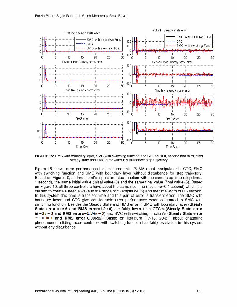
Farzin Piltan, Sajad Rahmdel, Saleh Mehrara & Reza Bayat
International Journal of Engineering (IJE), Volume (6) : Issue (3) : 2012 166
FIGURE 15: SMC with boundary layer, SMC with switching function and CTC for first, second and third joints
steady state and RMS error without disturbance: step trajectory
Figure 15 shows error performance for first three links PUMA robot manipulator in CTC, SMC with switching function and SMC with boundary layer without disturbance for step trajectory. Based on Figure 10, all three joint’s inputs are step function with the same step time (step time= 1 second), the same initial value (initial value=0) and the same final value (final value=5). Based on Figure 10, all three controllers have about the same rise time (rise time=0.4 second) which it is caused to create a needle wave in the range of 5 (amplitude=5) and the time width of 0.6 second. In this system this time is transient time and this part of error is transient error. The SMC with boundary layer and CTC give considerable error performance when compared to SMC with switching function. Besides the Steady State and RMS error in SMC with boundary layer (Steady State error =1e-6 and RMS error=1.2e-6) are fairly lower than CTC’s (Steady State error
and RMS error= ) and SMC with switching function’s (Steady State error and RMS error=0.00652). Based on literature [17-18, 20-21] about chattering
phenomenon, sliding mode controller with switching function has fairly oscillation in this system without any disturbance.

Farzin Piltan, Sajad Rahmdel, Saleh Mehrara & Reza Bayat
International Journal of Engineering (IJE), Volume (6) : Issue (3) : 2012 167
FIGURE 16: SMC with boundary layer, SMC with switching function and CTC First, second and third link steady state and RMS error with disturbance: step trajectory
Figure 16 shows steady state and RMS error performance for first three links PUMA robot manipulator in CTC, SMC with switching function and SMC with boundary layer with 40% disturbance for step trajectory. Based on Figure 10, all three joint’s inputs are step function with the same step time (step time= 1 second), the same initial value (initial value=0) and the same final value (final value=5). Based on Figure 10, all three controllers have about the same rise time (rise time=0.4 second) which it is caused to create a needle wave in the range of 5 (amplitude=5) and the time width of 0.6 second. In this system this time is transient time and this part of error is transient error. The SMC with boundary layer gives considerable error performance when compared to CTC and SMC with switching function. Besides the Steady State and RMS error in SMC with boundary layer (Steady State error =10e-5 and RMS error=11e-4) are fairly lower
than CTC’s (Steady State error and RMS error= ) and SMC with switching function’s (Steady State error and RMS error=0.98). Based on Figure 16, all three controllers have oscillation in error response with regard to 40% of the input signal amplitude disturbance. When applied 40% disturbances in SMC with boundary layer the RMS error increased approximately 9.17% (percent of increase the steady state
error= ) and in CTC the RMS error increased
approximately 56% (percent of increase the steady state
error= ).
Chattering Phenomenon Chattering is one of the most important challenges in sliding mode controller therefore reducing the chattering is a major objective in this research. Chattering phenomenon is caused to the hitting in driver and mechanical parts therefore reduce the chattering is very important in this research. To reduce the chattering this research is focused on function instead of
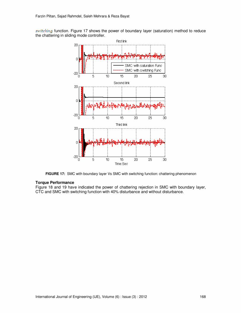
Farzin Piltan, Sajad Rahmdel, Saleh Mehrara & Reza Bayat
International Journal of Engineering (IJE), Volume (6) : Issue (3) : 2012 168
function. Figure 17 shows the power of boundary layer (saturation) method to reduce the chattering in sliding mode controller.
FIGURE 17: SMC with boundary layer Vs SMC with switching function: chattering phenomenon
Torque Performance Figure 18 and 19 have indicated the power of chattering rejection in SMC with boundary layer, CTC and SMC with switching function with 40% disturbance and without disturbance.

Farzin Piltan, Sajad Rahmdel, Saleh Mehrara & Reza Bayat
International Journal of Engineering (IJE), Volume (6) : Issue (3) : 2012 169
FIGURE 18: SMC with boundary layer, SMC with switching function and CTC for first, second and third joints
torque performance without disturbance
Figure 18 shows torque performance for first three links PUMA robot manipulator in CTC, SMC with switching function and SMC with boundary layer without disturbance. Based on Figure 18, The SMC with boundary layer and CTC give considerable torque performance when compared to SMC with switching function. Figure 19 have indicated the robustness in torque performance for first three links PUMA robot manipulator in CTC, SMC with switching function and SMC with boundary layer in presence of 40% disturbance. In this research boundary layer sliding mode controller has the steady torque oscillation in presence of external disturbance compared to CTC and SMC with switching function therefore SMC with boundary layer is more robust then the other two controllers.

Farzin Piltan, Sajad Rahmdel, Saleh Mehrara & Reza Bayat
International Journal of Engineering (IJE), Volume (6) : Issue (3) : 2012 170
FIGURE 19: SMC with boundary layer, SMC with switching function and CTC for first, second and third link joints performance with40% disturbance
Based on Figure 19, it is observed that however all of three controllers have oscillation but SMC with boundary layer has better performance compared to CTC and SMC with switching function in presence of 40% disturbance. This is mainly because SMC with saturation function is more robust than CTC and SMC with switching function. Oscillation for all three controllers is increased but SMC with saturation function is more robust however is not still must be improved. In this part SMC with saturation function, CTC and SMC with switching function have been comparatively evaluation through MATLAB simulation, for PUMA robot manipulator control. It is observed that the SMC with saturation function gives the best performance in presence of uncertainties and external disturbance.
6. CONCLUSION Refer to this research, position sliding mode controller (SMC) and computed torque controller (CTC) are proposed for PUMA robot manipulator. The first problem of the pure sliding mode controller with switching function was chattering phenomenon in certain and uncertain systems. The chattering phenomenon problem can be reduced in certain system by using linear saturation boundary layer function in sliding mode control law. The simulation results exhibit that the sliding mode controller with saturation function works well in certain system. This methodology is based on applied saturation function in sliding mode methodology to estimate chattering phenomenon. The results demonstrate that the sliding mode controller with saturation function is a model-based controllers which works well in certain and partly uncertain system. The stability and convergence of the sliding mode controller based on switching function is guarantee and proved by the Lyapunov method. Based on theoretical and simulation results, it is observed that sliding mode controller is more robust than computed torque controller for robot manipulator.

Farzin Piltan, Sajad Rahmdel, Saleh Mehrara & Reza Bayat
International Journal of Engineering (IJE), Volume (6) : Issue (3) : 2012 171
REFERENCES [1] T. R. Kurfess, Robotics and automation handbook: CRC, 2005. [2] J. J. E. Slotine and W. Li, Applied nonlinear control vol. 461: Prentice hall Englewood Cliffs,
NJ, 1991. [3] K. Ogata, Modern control engineering: Prentice Hall, 2009. [4] L. Cheng, Z. G. Hou, M. Tan, D. Liu and A. M. Zou, "Multi-agent based adaptive consensus
control for multiple manipulators with kinematic uncertainties," 2008, pp. 189-194. [5] J. J. D'Azzo, C. H. Houpis and S. N. Sheldon, Linear control system analysis and design
with MATLAB: CRC, 2003. [6] B. Siciliano and O. Khatib, Springer handbook of robotics: Springer-Verlag New York Inc,
2008. [7] I. Boiko, L. Fridman, A. Pisano and E. Usai, "Analysis of chattering in systems with second-
order sliding modes," IEEE Transactions on Automatic Control, No. 11, vol. 52,pp. 2085-2102, 2007.
[8] J. Wang, A. Rad and P. Chan, "Indirect adaptive fuzzy sliding mode control: Part I: fuzzy
switching," Fuzzy Sets and Systems, No. 1, vol. 122,pp. 21-30, 2001. [9] C. Wu, "Robot accuracy analysis based on kinematics," IEEE Journal of Robotics and
Automation, No. 3, vol. 2, pp. 171-179, 1986. [10] H. Zhang and R. P. Paul, "A parallel solution to robot inverse kinematics," IEEE conference
proceeding, 2002, pp. 1140-1145. [11] J. Kieffer, "A path following algorithm for manipulator inverse kinematics," IEEE conference
proceeding, 2002, pp. 475-480. [12] Z. Ahmad and A. Guez, "On the solution to the inverse kinematic problem(of robot)," IEEE
conference proceeding, 1990, pp. 1692-1697. [13] F. T. Cheng, T. L. Hour, Y. Y. Sun and T. H. Chen, "Study and resolution of singularities for
a 6-DOF PUMA manipulator," Systems, Man, and Cybernetics, Part B: Cybernetics, IEEE Transactions on, No. 2, vol. 27, pp. 332-343, 2002.
[14] M. W. Spong and M. Vidyasagar, Robot dynamics and control: Wiley-India, 2009. [15] A. Vivas and V. Mosquera, "Predictive functional control of a PUMA robot," Conference
Proceedings, 2005. [16] D. Nguyen-Tuong, M. Seeger and J. Peters, "Computed torque control with nonparametric
regression models," IEEE conference proceeding, 2008, pp. 212-217. [17] V. Utkin, "Variable structure systems with sliding modes," Automatic Control, IEEE
Transactions on, No. 2, vol. 22, pp. 212-222, 2002. [18] R. A. DeCarlo, S. H. Zak and G. P. Matthews, "Variable structure control of nonlinear
multivariable systems: a tutorial," Proceedings of the IEEE, No. 3, vol. 76, pp. 212-232, 2002.

Farzin Piltan, Sajad Rahmdel, Saleh Mehrara & Reza Bayat
International Journal of Engineering (IJE), Volume (6) : Issue (3) : 2012 172
[19] K. D. Young, V. Utkin and U. Ozguner, "A control engineer's guide to sliding mode control," IEEE conference proceeding, 2002, pp. 1-14.
[20] O. Kaynak, "Guest editorial special section on computationally intelligent methodologies and
sliding-mode control," IEEE Transactions on Industrial Electronics, No. 1, vol. 48, pp. 2-3, 2001.
[21] J. J. Slotine and S. Sastry, "Tracking control of non-linear systems using sliding surfaces,
with application to robot manipulators†," International Journal of Control, No. 2, vol. 38, pp. 465-492, 1983.
[22] J. J. E. Slotine, "Sliding controller design for non-linear systems," International Journal of
Control, No. 2, vol. 40, pp. 421-434, 1984. [23] R. Palm, "Sliding mode fuzzy control," IEEE conference proceeding,2002, pp. 519-526. [24] C. C. Weng and W. S. Yu, "Adaptive fuzzy sliding mode control for linear time-varying
uncertain systems," IEEE conference proceeding, 2008, pp. 1483-1490. [25] M. Ertugrul and O. Kaynak, "Neuro sliding mode control of robotic manipulators,"
Mechatronics Journal, No. 1, vol. 10, pp. 239-263, 2000. [26] P. Kachroo and M. Tomizuka, "Chattering reduction and error convergence in the sliding-
mode control of a class of nonlinear systems," Automatic Control, IEEE Transactions on, No. 7, vol. 41, pp. 1063-1068, 2002.
[27] H. Elmali and N. Olgac, "Implementation of sliding mode control with perturbation estimation
(SMCPE)," Control Systems Technology, IEEE Transactions on, No. 1, vol. 4, pp. 79-85, 2002.
[28] J. Moura and N. Olgac, "A comparative study on simulations vs. experiments of SMCPE,"
IEEE conference proceeding, 2002, pp. 996-1000. [29] Y. Li and Q. Xu, "Adaptive Sliding Mode Control With Perturbation Estimation and PID
Sliding Surface for Motion Tracking of a Piezo-Driven Micromanipulator," Control Systems Technology, IEEE Transactions on, No. 4, vol. 18, pp. 798-810, 2010.
[30] B. Wu, Y. Dong, S. Wu, D. Xu and K. Zhao, "An integral variable structure controller with
fuzzy tuning design for electro-hydraulic driving Stewart platform," IEEE conference proceeding, 2006, pp. 5-945.
[31] Farzin Piltan , N. Sulaiman, Zahra Tajpaykar, Payman Ferdosali, Mehdi Rashidi, “Design
Artificial Nonlinear Robust Controller Based on CTLC and FSMC with Tunable Gain,” International Journal of Robotic and Automation, 2 (3): 205-220, 2011.
[32] Farzin Piltan, A. R. Salehi and Nasri B Sulaiman.,” Design artificial robust control of second
order system based on adaptive fuzzy gain scheduling,” world applied science journal (WASJ), 13 (5): 1085-1092, 2011.
[33] Farzin Piltan, N. Sulaiman, Atefeh Gavahian, Samira Soltani, Samaneh Roosta, “Design
Mathematical Tunable Gain PID-Like Sliding Mode Fuzzy Controller with Minimum Rule Base,” International Journal of Robotic and Automation, 2 (3): 146-156, 2011.
[34] Farzin Piltan , A. Zare, Nasri B. Sulaiman, M. H. Marhaban and R. Ramli, , “A Model Free
Robust Sliding Surface Slope Adjustment in Sliding Mode Control for Robot Manipulator,” World Applied Science Journal, 12 (12): 2330-2336, 2011.

Farzin Piltan, Sajad Rahmdel, Saleh Mehrara & Reza Bayat
International Journal of Engineering (IJE), Volume (6) : Issue (3) : 2012 173
[35] Farzin Piltan , A. H. Aryanfar, Nasri B. Sulaiman, M. H. Marhaban and R. Ramli “Design
Adaptive Fuzzy Robust Controllers for Robot Manipulator,” World Applied Science Journal, 12 (12): 2317-2329, 2011.
[36] Farzin Piltan, N. Sulaiman , Arash Zargari, Mohammad Keshavarz, Ali Badri , “Design PID-
Like Fuzzy Controller With Minimum Rule Base and Mathematical Proposed On-line Tunable Gain: Applied to Robot Manipulator,” International Journal of Artificial intelligence and expert system, 2 (4):184-195, 2011.
[37] Farzin Piltan, Nasri Sulaiman, M. H. Marhaban and R. Ramli, “Design On-Line Tunable Gain
Artificial Nonlinear Controller,” Journal of Advances In Computer Research, 2 (4): 75-83, 2011.
[38] Farzin Piltan, N. Sulaiman, Payman Ferdosali, Iraj Assadi Talooki, “ Design Model Free
Fuzzy Sliding Mode Control: Applied to Internal Combustion Engine,” International Journal of Engineering, 5 (4):302-312, 2011.
[39] Farzin Piltan, N. Sulaiman, Samaneh Roosta, M.H. Marhaban, R. Ramli, “Design a New
Sliding Mode Adaptive Hybrid Fuzzy Controller,” Journal of Advanced Science & Engineering Research , 1 (1): 115-123, 2011.
[40] Farzin Piltan, Atefe Gavahian, N. Sulaiman, M.H. Marhaban, R. Ramli, “Novel Sliding Mode
Controller for robot manipulator using FPGA,” Journal of Advanced Science & Engineering Research, 1 (1): 1-22, 2011.
[41] Farzin Piltan, N. Sulaiman, A. Jalali & F. Danesh Narouei, “Design of Model Free Adaptive
Fuzzy Computed Torque Controller: Applied to Nonlinear Second Order System,” International Journal of Robotics and Automation, 2 (4):232-244, 2011.
[42] Farzin Piltan, N. Sulaiman, Iraj Asadi Talooki, Payman Ferdosali, “Control of IC Engine:
Design a Novel MIMO Fuzzy Backstepping Adaptive Based Fuzzy Estimator Variable Structure Control ,” International Journal of Robotics and Automation, 2 (5):360-380, 2011.
[43] Farzin Piltan, N. Sulaiman, Payman Ferdosali, Mehdi Rashidi, Zahra Tajpeikar, “Adaptive
MIMO Fuzzy Compensate Fuzzy Sliding Mode Algorithm: Applied to Second Order Nonlinear System,” International Journal of Engineering, 5 (5): 380-398, 2011.
[44] Farzin Piltan, N. Sulaiman, Hajar Nasiri, Sadeq Allahdadi, Mohammad A. Bairami, “Novel
Robot Manipulator Adaptive Artificial Control: Design a Novel SISO Adaptive Fuzzy Sliding Algorithm Inverse Dynamic Like Method,” International Journal of Engineering, 5 (5): 399-418, 2011.
[45] Farzin Piltan, N. Sulaiman, Sadeq Allahdadi, Mohammadali Dialame, Abbas Zare, “Position
Control of Robot Manipulator: Design a Novel SISO Adaptive Sliding Mode Fuzzy PD Fuzzy Sliding Mode Control,” International Journal of Artificial intelligence and Expert System, 2 (5):208-228, 2011.
[46] Farzin Piltan, SH. Tayebi HAGHIGHI, N. Sulaiman, Iman Nazari, Sobhan Siamak, “Artificial
Control of PUMA Robot Manipulator: A-Review of Fuzzy Inference Engine And Application to Classical Controller ,” International Journal of Robotics and Automation, 2 (5):401-425, 2011.
[47] Farzin Piltan, N. Sulaiman, Abbas Zare, Sadeq Allahdadi, Mohammadali Dialame, “Design
Adaptive Fuzzy Inference Sliding Mode Algorithm: Applied to Robot Arm,” International Journal of Robotics and Automation , 2 (5): 283-297, 2011.
Farzin Piltan, Sajad Rahmdel, Saleh Mehrara & Reza Bayat
International Journal of Engineering (IJE), Volume (6) : Issue (3) : 2012 174
[48] Farzin Piltan, Amin Jalali, N. Sulaiman, Atefeh Gavahian, Sobhan Siamak, “Novel Artificial Control of Nonlinear Uncertain System: Design a Novel Modified PSO SISO Lyapunov Based Fuzzy Sliding Mode Algorithm ,” International Journal of Robotics and Automation, 2 (5): 298-316, 2011.
[49] Farzin Piltan, N. Sulaiman, Amin Jalali, Koorosh Aslansefat, “Evolutionary Design of
Mathematical tunable FPGA Based MIMO Fuzzy Estimator Sliding Mode Based Lyapunov Algorithm: Applied to Robot Manipulator,” International Journal of Robotics and Automation, 2 (5):317-343, 2011.
[50] Farzin Piltan, N. Sulaiman, Samaneh Roosta, Atefeh Gavahian, Samira Soltani,
“Evolutionary Design of Backstepping Artificial Sliding Mode Based Position Algorithm: Applied to Robot Manipulator,” International Journal of Engineering, 5 (5):419-434, 2011.
[51] Farzin Piltan, N. Sulaiman, S.Soltani, M. H. Marhaban & R. Ramli, “An Adaptive sliding
surface slope adjustment in PD Sliding Mode Fuzzy Control for Robot Manipulator,” International Journal of Control and Automation , 4 (3): 65-76, 2011.
[52] Farzin Piltan, N. Sulaiman, Mehdi Rashidi, Zahra Tajpaikar, Payman Ferdosali, “Design and
Implementation of Sliding Mode Algorithm: Applied to Robot Manipulator-A Review ,” International Journal of Robotics and Automation, 2 (5):265-282, 2011.
[53] Farzin Piltan, N. Sulaiman, Amin Jalali, Sobhan Siamak, and Iman Nazari, “Control of Robot
Manipulator: Design a Novel Tuning MIMO Fuzzy Backstepping Adaptive Based Fuzzy Estimator Variable Structure Control ,” International Journal of Control and Automation, 4 (4):91-110, 2011.
[54] Farzin Piltan, N. Sulaiman, Atefeh Gavahian, Samaneh Roosta, Samira Soltani, “On line
Tuning Premise and Consequence FIS: Design Fuzzy Adaptive Fuzzy Sliding Mode Controller Based on Lyaponuv Theory,” International Journal of Robotics and Automation, 2 (5):381-400, 2011.
[55] Farzin Piltan, N. Sulaiman, Samaneh Roosta, Atefeh Gavahian, Samira Soltani, “Artificial
Chattering Free on-line Fuzzy Sliding Mode Algorithm for Uncertain System: Applied in Robot Manipulator,” International Journal of Engineering, 5 (5):360-379, 2011.
[56] Farzin Piltan, N. Sulaiman and I.AsadiTalooki, “Evolutionary Design on-line Sliding Fuzzy
Gain Scheduling Sliding Mode Algorithm: Applied to Internal Combustion Engine,” International Journal of Engineering Science and Technology, 3 (10):7301-7308, 2011.
[57] Farzin Piltan, Nasri B Sulaiman, Iraj Asadi Talooki and Payman Ferdosali.,” Designing On-
Line Tunable Gain Fuzzy Sliding Mode Controller Using Sliding Mode Fuzzy Algorithm: Applied to Internal Combustion Engine,” world applied science journal (WASJ), 15 (3): 422-428, 2011.
[58] B. K. Yoo and W. C. Ham, "Adaptive control of robot manipulator using fuzzy compensator,"
Fuzzy Systems, IEEE Transactions on, No. 2, vol. 8, pp. 186-199, 2002. [59] H. Medhaffar, N. Derbel and T. Damak, "A decoupled fuzzy indirect adaptive sliding mode
controller with application to robot manipulator," International Journal of Modelling, Identification and Control, No. 1, vol. 1, pp. 23-29, 2006.
[60] Y. Guo and P. Y. Woo, "An adaptive fuzzy sliding mode controller for robotic manipulators,"
Systems, Man and Cybernetics, Part A: Systems and Humans, IEEE Transactions on, No. 2, vol. 33, pp. 149-159, 2003.

Farzin Piltan, Sajad Rahmdel, Saleh Mehrara & Reza Bayat
International Journal of Engineering (IJE), Volume (6) : Issue (3) : 2012 175
[61] C. M. Lin and C. F. Hsu, "Adaptive fuzzy sliding-mode control for induction servomotor systems," Energy Conversion, IEEE Transactions on, No. 2, vol. 19, pp. 362-368, 2004.
[62] N. Sulaiman, Z. A. Obaid, M. Marhaban and M. Hamidon , "Design and Implementation of
FPGA-Based Systems-A Review," Australian Journal of Basic and Applied Sciences, No. 4, vol. 3, pp. 3575-3596, 2009.
[63] X. Shao and D. Sun, "Development of an FPGA-based motion control ASIC for robotic
manipulators," IEEE Conference , 2006, pp. 8221-8225. [64] Y. S. Kung, K. Tseng, C. Chen, H. Sze and A. Wang, "FPGA-implementation of inverse
kinematics and servo controller for robot manipulator," Proc. IEEE Int. on Robotics and Biomimetics, pp. 1163–1168, 2006.
[65] X. Shao, D. Sun and J. K. Mills, "A new motion control hardware architecture with FPGA-
based IC design for robotic manipulators," IEEE Conference, 2006, pp. 3520-3525. [66] Y. S. Kung, C. S. Chen and G. S. Shu, "Design and Implementation of a Servo System for
Robotic Manipulator," CACS, 2005. [67] U. D. Meshram and R. Harkare, "FPGA Based Five Axis Robot Arm Controller," IEEE
Conference, 2005, pp. 3520-3525. [68] U. Meshram, P. Bande, P. Dwaramwar and R. Harkare, "Robot arm controller using FPGA,"
IEEE Conference, 2009, pp. 8-11. [69] Y. S. Kung and G. S. Shu, "Development of a FPGA-based motion control IC for robot arm,"
IEEE Conference, 2006, pp. 1397-1402. [70] Z. A. Obaid, N. Sulaiman and M. Hamidon, "Developed Method of FPGA-based Fuzzy Logic
Controller Design with the Aid of Conventional PID Algorithm," Australian Journal of Basic and Applied Sciences, No. 3, vol. 3, pp. 2724-2740, 2009.
[71] S. T. Karris, Digital circuit analysis and design with Simulink modeling and introduction to
CPLDs and FPGAs: Orchard Pubns, 2007. [72] K. D. Rogers, "Acceleration and implementation of a DSP phase-based frequency
estimation algorithm: MATLAB/SIMULINK to FPGA via XILINX system generator," Citeseer, 2004.
[73] F. J. Lin, D. H. Wang and P. K. Huang, "FPGA-based fuzzy sliding-mode control for a linear
induction motor drive," IEEE journal of electrical power application, No. 5, Vol. 152, 2005, pp. 1137-1148.
[74] R. R. Ramos, D. Biel, E. Fossas and F. Guinjoan, "A fixed-frequency quasi-sliding control
algorithm: application to power inverters design by means of FPGA implementation," Power Electronics, IEEE Transactions on, No. 1, vol. 18, pp. 344-355, 2003.
[75] Xiaosong. Lu, "An investigation of adaptive fuzzy sliding mode control for robot manipulator,"
Carleton university Ottawa,2007. [76] S. Lentijo, S. Pytel, A. Monti, J. Hudgins, E. Santi and G. Simin, "FPGA based sliding mode
control for high frequency power converters," IEEE Conference, 2004, pp. 3588-3592. [77] B. S. R. Armstrong, "Dynamics for robot control: friction modeling and ensuring excitation
during parameter identification," 1988.
Farzin Piltan, Sajad Rahmdel, Saleh Mehrara & Reza Bayat
International Journal of Engineering (IJE), Volume (6) : Issue (3) : 2012 176
[78] C. L. Clover, "Control system design for robots used in simulating dynamic force and
moment interaction in virtual reality applications," 1996. [79] K. R. Horspool, Cartesian-space Adaptive Control for Dual-arm Force Control Using
Industrial Robots: University of New Mexico, 2003. [80] B. Armstrong, O. Khatib and J. Burdick, "The explicit dynamic model and inertial parameters
of the PUMA 560 arm," IEEE Conference, 2002, pp. 510-518. [81] P. I. Corke and B. Armstrong-Helouvry, "A search for consensus among model parameters
reported for the PUMA 560 robot," IEEE Conference, 2002, pp. 1608-1613. [82] Farzin Piltan, N. Sulaiman, M. H. Marhaban, Adel Nowzary, Mostafa Tohidian,” “Design of
FPGA based sliding mode controller for robot manipulator,” International Journal of Robotic and Automation, 2 (3): 183-204, 2011.
[83] I. Eksin, M. Guzelkaya and S. Tokat, "Sliding surface slope adjustment in fuzzy sliding mode
controller," Mediterranean Conference, 2002, pp. 160-168. [84] Samira Soltani & Farzin Piltan, “Design Artificial Nonlinear Controller Based on Computed
Torque like Controller with Tunable Gain”. World Applied Science Journal,14 (9): 1306-1312, 2011.
[85] Farzin Piltan, H. Rezaie, B. Boroomand, Arman Jahed,” Design robust back stepping online
tuning feedback linearization control applied to IC engine,” International Journal of
Advance Science and Technology, 42: 183-204, 2012.
[86] Farzin Piltan, I. Nazari, S. Siamak, P. Ferdosali ,”Methodology of FPGA-based
mathematical error-based tuning sliding mode controller” International Journal of Control
and Automation, 5(1): 89-110, 2012.
[87] Farzin Piltan, M. A. Dialame, A. Zare, A. Badri ,”Design Novel Lookup table changed Auto
Tuning FSMC: Applied to Robot Manipulator” International Journal of Engineering, 6(1):
25-40, 2012.
[88] Farzin Piltan, B. Boroomand, A. Jahed, H. Rezaie ,”Methodology of Mathematical Error-
Based Tuning Sliding Mode Controller” International Journal of Engineering, 6(2): 96-112,
2012.
[89] Farzin Piltan, F. Aghayari, M. R. Rashidian, M. Shamsodini, ”A New Estimate Sliding Mode
Fuzzy Controller for Robotic Manipulator” International Journal of Robotics and
Automation, 3(1): 45-58, 2012.
[90] Farzin Piltan, M. Keshavarz, A. Badri, A. Zargari , ”Design novel nonlinear controller applied
to robot manipulator: design new feedback linearization fuzzy controller with minimum rule
base tuning method” International Journal of Robotics and Automation, 3(1): 1-18, 2012.
[91] Piltan, F., et al. "Design sliding mode controller for robot manipulator with artificial tunable
gain". Canaidian Journal of pure and applied science, 5 (2), 1573-1579, 2011.

Farzin Piltan, Sajad Rahmdel, Saleh Mehrara & Reza Bayat
International Journal of Engineering (IJE), Volume (6) : Issue (3) : 2012 177
[92] Farzin Piltan, A. Hosainpour, E. Mazlomian, M.Shamsodini, M.H Yarmahmoudi. ”Online Tuning Chattering Free Sliding Mode Fuzzy Control Design: Lyapunov Approach” International Journal of Robotics and Automation, 3(3): 2012.
[93] Farzin Piltan , M.H. Yarmahmoudi, M. Shamsodini, E.Mazlomian, A.Hosainpour. ” PUMA-
560 Robot Manipulator Position Computed Torque Control Methods Using MATLAB/SIMULINK and Their Integration into Graduate Nonlinear Control and MATLAB Courses” International Journal of Robotics and Automation, 3(3): 2012.
[94] Farzin Piltan, R. Bayat, F. Aghayari, B. Boroomand. “Design Error-Based Linear Model-
Free Evaluation Performance Computed Torque Controller” International Journal of Robotics and Automation, 3(3): 2012.
[95] Farzin Piltan, S. Emamzadeh, Z. Hivand, F. Shahriyari & Mina Mirazaei . ” PUMA-560 Robot
Manipulator Position Sliding Mode Control Methods Using MATLAB/SIMULINK and Their Integration into Graduate/Undergraduate Nonlinear Control, Robotics and MATLAB Courses” International Journal of Robotics and Automation, 3(3): 2012.
[96] Farzin Piltan, J. Meigolinedjad, S. Mehrara, S. Rahmdel. ” Evaluation Performance of 2
nd
Order Nonlinear System: Baseline Control Tunable Gain Sliding Mode Methodology” International Journal of Robotics and Automation, 3(3): 2012.
[97] Farzin Piltan, M. Mirzaie, F. Shahriyari, Iman Nazari & S. Emamzadeh.” Design Baseline Computed Torque Controller” International Journal of Engineering, 3(3): 2012.

Md. Moniruzzaman, Md. Murad Kabir Nipun & Sajib Roy
International Journal of Engineering (IJE), Volume (6) : Issue (3) : 2012 178
Extremely Low Power FIR Filter for a Smart Dust Sensor Module
Md. Moniruzzaman [email protected] Department of Electronics & Telecommunication Engineering Southeast University Dhaka, 1207, Bangladesh
Md. Murad Kabir Nipun [email protected] Department of Electrical & Electronic Engineering Southeast University Dhaka, 1207, Bangladesh
Sajib Roy [email protected] Department of Electronics & Telecommunication Engineering University of Liberal Arts Bangladesh Dhaka, 1209, Bangladesh
Abstract
Digital filters are common components in many applications today, also in for sensor systems, such as large-scale distributed smart dust sensors. For these applications the power consumption is very critical, it has to be extremely low. With the transistor technology scaling becoming more and more sensitive to e.g. gate leakage, it has become a necessity to find ways to minimize the flow of leakage in current CMOS logic. This paper studies sub-threshold source coupled logic (STSCL) in a 45-nm process. The STSCL can be used instead of traditional CMOS to meet the low power and energy consumption requirements. The STSCL style is in this paper used to design a digital filter, applicable for the audio interface of a smart dust sensor where the sample frequency will be 44.1 kHz. A finite-length impulse response (FIR) filter is used with transposed direct form structure and for the coefficient multiplication five-bit canonic signed digit [7] based serial/parallel multipliers were used. The power consumption is calculated along with the delay in order to present the power delay product (PDP) such that the performance of the sub-threshold logic can be compared with corresponding CMOS implementation. The simulated results shows a significant reduction in energy consumption (in terms of PDP) with the system running at a supply voltage as low as 0.2 V using STSCL. Keywords: STSCL, CMOS, PDP, CSD Multiplier, FIR Filter.
1. INTRODUCTION
This Smart dust is a new and emerging technology in the fields of small wireless sensor development. They are very small and each sensor has the capability of communicating with other sensors. They are run by battery power supply and its lifetime depends on the application and environment it is being used by. Currently these sensors are applied in forest services and in chemical plants. The basic purpose of these sensors are to gather important data (excluding noise or unwanted data) from the environment it is being applied to, and then transfer them to a main server by wireless medium. It has basic DSP (digital signal processing) sections to perform processing of the gathered input signals. One of the key components of that DSP section is a digital filter which is required for eliminating any unwanted signals or noise. It is important for the longevity of these sensors that they should consume as low power/energy during application (without degrading performance by too much) and have a long lasting battery life. For achieving such longevity in respect to battery life, the digital sections of these sensors need to be run under lower supply and also dissipate as low leakage as possible. But it has to be kept in mind system performance or delay must not be harmed by great amount in the course of reducing supply voltage. Thus low power and low energy consumption with desirable performance are highly
Md. Moniruzzaman, Md. Murad Kabir Nipun & Sajib Roy
International Journal of Engineering (IJE), Volume (6) : Issue (3) : 2012 179
demanding requirements in the field of small-scale sensor applications. Integrated circuitry used in these types of sensors must be efficiently employed and optimized such that the overall system consumes very low energy from its battery or source of energy without any or with minor degradation of performance. For current MOSFET processes at channel lengths below 65 nm the leakage currents and its impact on performance has become a factor of concern. At a 45 nm node, or below, the trend is that the leakage current continues to have a negative impact on performance as well as the energy consumption. The usage of dynamic voltage scaling can reduce the dynamic energy dissipation, but quite often this also increase the leakage current. Further on, in 45 nm or lower the gate-to-channel tunneling effects is a large contributor to the overall energy consumption. Leakage current can also consist of subthreshold leakage, which is significant during the off-state operation mode. In CMOS the sub-threshold leakage can be reduced by using MOSFET devices with high threshold value which in turn narrows down the possible range for voltage scaling. Further on, reducing supply voltage in attempt to reduce power consumption has a drawback as it increases the propagation delay. So even though power consumption is less but due to larger delay - the energy consumption of the system increases, hence performance as well as battery life for the system degrades. The mentioned drawbacks can be solved using several different techniques like power gating [1] or multi-threshold CMOS libraries [2]. In some sense, this increases the design complexity and imposes difficulties for the verification and verification tools. For example, we might have to introduce several different clock domains and power modes/domains to maintain the system performance under all conditions. Thus the use of new types of logic styles, instead of CMOS, is a welcomed approach. Sub-threshold source coupled logic (STSCL) is a fairly new kind of logic style that have recently came into consideration for its ability to operate and perform at sub- threshold region (Vin < Vt) of a MOSFET device [3]. This operating ability at sub-threshold or linear region allows the use of gates implemented with STSCL and they can be operated at very low supply voltage without little harm on system performance. Thus providing a low energy consumption rate for a system implemented with STSCL gates. The understandings of the STSCL topology is applied to a fifth-order FIR transposed direct form filter. We are aware that FIR filters might require more computational power, but as we are focusing on observing the advantages of using STSCL topology over CMOS in terms of energy consumption, this type of filter architecture is better suited for serving the purpose. The basic STSCL inverter circuit and the required bias circuit for operating the logic at sub-threshold region have already been designed and tested in other research papers [1]. Thereby focus in this specific paper is given on the STSCL implemented gates needed for filter designing, and the minimal configuration at which the gates can operate suitably. Section II and III insights on the implementation of the STSCL based gates, the amplifier needed for the replica bias circuit and the 5th order filter in STSCL gates. Finally the paper concludes with the comparison of their performance with CMOS gate implementation.
2. BASIC LOGIC GATES IN STSCL
The Exclusive or (XOR/XNOR), or (OR/NOR), and (AND/NAND) gates, along with flip-flops (DFF/DNFF) are the most commonly required logic gates to design a digital filter that will be applicable to smart dust sensor modules implementation. The logic gates are designed to perform under sub-threshold region at scaled down supply voltages; down to 0.2 V. The provided bias currents per stage are in the order of 250 pA. The PMOS (acting as high resistive load [4]) widths are 135 nm (has to be low in order to achieve a high load resistive value, this is mandatory for running the gates at sub-threshold region) and the NMOS input devices are off widths 675 as they need to have stronger driving capability to perform full logic swing of the next logic stages.. The circuit schematics for the XOR, OR, AND gates and DFF are given in Figure 1. The results of performed simulations on XOR, OR and AND given in TABLE 1. The simulations are performed with inputs at a rate of 10 kHz. For the DFF a clock frequency of 44.1 kHz is applied with the input data rate at 10 kHz, like before, and an output duty factor of 50 %.

Md. Moniruzzaman, Md. Murad Kabir Nipun & Sajib Roy
International Journal of Engineering (IJE), Volume (6) : Issue (3) : 2012 180
Logic Temperature Power[nW] Delay [µs] XOR/XNOR - 20 0.152 2.52
70 1.11 0.096 OR/NOR -20 0.157 1.489
70 1.15 0.129 AND/NAND -20 0.15 1.422
70 1.15 0.135 DFF -20 0.442 2.97
Logic Temperature Power[nW] Delay [µs] DFF 70 3.366 0.152
TABLE 1: Power-Delay table for STSCL based logic gates
FIGURE 1: XOR/XNOR, OR/NOR, AND/NAND, DFF
2.1 Sub-threshold Amplifier for Bias Circuit [1] Folded-cascode architecture has been used to design the amplifier required for the design of replica bias circuit. In Figure 2 shows a schematic view of the amplifier with modified PMOS load device [4]. Similar PMOS load devices have been used for the design of the amplifier's

Md. Moniruzzaman, Md. Murad Kabir Nipun & Sajib Roy
International Journal of Engineering (IJE), Volume (6) : Issue (3) : 2012 181
architecture in order to operate it at sub-threshold region. Even-though this architecture uses more number of transistors but it can easily be applicable to operate at very low voltage. Other architectures like two-stage OTA can also be used which require less number of transistors but is difficult to be operated at sub-threshold regime.
FIGURE 2: Folded-cascode amplifier (operates in sub-threshold region)
3. STSCL BASED FIR FILTER The fifth order FIR filter designed in this paper is a conventional, widely-used and foremost verified structure (as in Figure 3). IIR filter can be also used instead of the FIR filter but IIR filters have more design complications compare to FIR filter. The filter has a of serial-input and serial-output form with a sampling frequency of 44.1 kHz, and for the multiplication with fixed coefficients a five-bit of serial/parallel multiplier [6] has been used. The response for the filter is given in Figure 4. The coefficients are represented in canonic signed digit (CSD) form. CSD is an optimized form compares to the more conventional two’s complement form [5]. The CSD based S/P multiplier uses lesser hardware resources and hence lower the power down to further level. The supply voltage is 0.2 V with a bias current at 250 pA per stage as discussed before. The supply voltage of 0.2 V is the limit up to which the system can be operated. The basic tryout for the different supplies allowed seeing how well a system could perform under critical situation while STSCL gates have been configured to run at their minimum operating specification. Simulations have been operated and compiled on Cadence Virtuoso v6.14, using both CMOS and STSCL at -20°C and 70°C temperature. The results of the PDP along with the delay for the fifth-order filter are shown in TABLE 2.
TABLE 2: PDP values for STSCL and CMOS based Fifth-order FIR filter.
Logic STSCL CMOS
Temp [°C] -20 70°C -20°C 70°C
PDP [fJ] 600.4 45.81 784.6 46.23 Delay [µs] Value 8 1.06 5.65 0.67
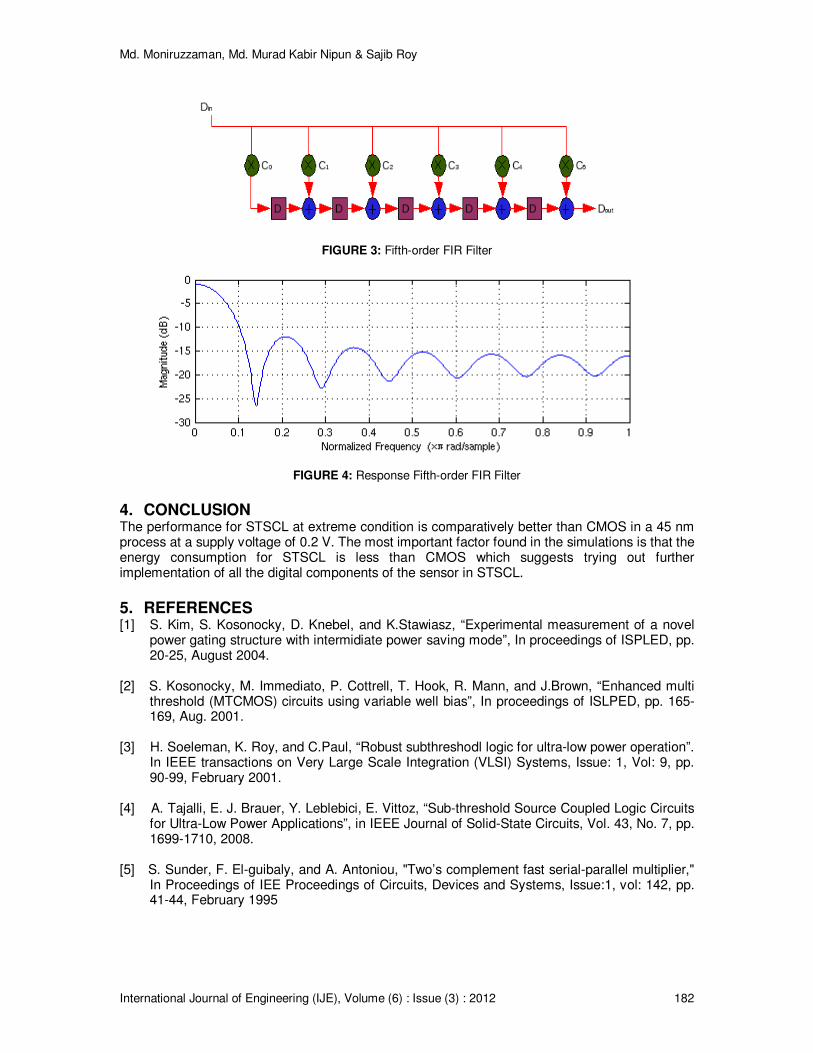
Md. Moniruzzaman, Md. Murad Kabir Nipun & Sajib Roy
International Journal of Engineering (IJE), Volume (6) : Issue (3) : 2012 182
FIGURE 3: Fifth-order FIR Filter
FIGURE 4: Response Fifth-order FIR Filter
4. CONCLUSION The performance for STSCL at extreme condition is comparatively better than CMOS in a 45 nm process at a supply voltage of 0.2 V. The most important factor found in the simulations is that the energy consumption for STSCL is less than CMOS which suggests trying out further implementation of all the digital components of the sensor in STSCL.
5. REFERENCES [1] S. Kim, S. Kosonocky, D. Knebel, and K.Stawiasz, “Experimental measurement of a novel
power gating structure with intermidiate power saving mode”, In proceedings of ISPLED, pp. 20-25, August 2004.
[2] S. Kosonocky, M. Immediato, P. Cottrell, T. Hook, R. Mann, and J.Brown, “Enhanced multi
threshold (MTCMOS) circuits using variable well bias”, In proceedings of ISLPED, pp. 165-169, Aug. 2001.
[3] H. Soeleman, K. Roy, and C.Paul, “Robust subthreshodl logic for ultra-low power operation”.
In IEEE transactions on Very Large Scale Integration (VLSI) Systems, Issue: 1, Vol: 9, pp. 90-99, February 2001.
[4] A. Tajalli, E. J. Brauer, Y. Leblebici, E. Vittoz, “Sub-threshold Source Coupled Logic Circuits
for Ultra-Low Power Applications”, in IEEE Journal of Solid-State Circuits, Vol. 43, No. 7, pp. 1699-1710, 2008.
[5] S. Sunder, F. El-guibaly, and A. Antoniou, "Two’s complement fast serial-parallel multiplier,"
In Proceedings of IEE Proceedings of Circuits, Devices and Systems, Issue:1, vol: 142, pp. 41-44, February 1995

Md. Moniruzzaman, Md. Murad Kabir Nipun & Sajib Roy
International Journal of Engineering (IJE), Volume (6) : Issue (3) : 2012 183
[6] M. Vesterbacka, K. Palmkvist, and L. Wanhammar, "Realization of Serial/Parallel Multipliers with Fixed Coefficients," In Proceedings of National Conf. on Radio Science, RVK'93, Lund Institute of Technology, Lund, Sweden, pp. 209-212, 5-7 April 1993.
[7] M. Hasan, J. Karam, M. Falkinburg, A Helwig and M. Ronning, "Canonic signed digit FIR
filter design," In Proceedings of 34th Asilomar Conference on Signals, Systems and
Computer, vol: 2, pp. 1653-1656, 29 October 2000.

A. E. Bakeri
International Journal of Engineering (IJE), Volume (6) : Issue (3) : 2012 184
Optimal Design of Hysteretic Dampers Connecting 2-MDOF Adjacent Structures for Random Excitations
A.E. Bakeri [email protected] Structural Eng. Dept., Faculty of Eng., Zagazig University Zagazig, Egypt
Abstract
The dynamic behaviour of two adjacent multi-degrees-of-freedom (MDOF) structures connected with a hysteretic damper is studied under base acceleration. The base acceleration is modeled as stationary white-noise random process. The governing equations of motion of the connected system are derived and solved using stochastic linearization technique. This study is concerned on the optimum design of the connecting dampers based on the minimization of the stored energy in the entire system. This procedure is applied on three models. The first is two adjacent three stories buildings, the second is ten stories buildings and the third is ten-story building adjacent to twenty-story building. The connecting damper is installed in three cases; in all floors, double dampers in different floors, and single damper. The results show that at these optimum properties of the connecting dampers, the response of each structure is reduced and the energy of the entire system is reduced. Keywords: Connected Structures, Stochastic Linearization, Hysteretic Damper, White-noise
1. INTRODUCTION Increasing the population and growing social and commercial activities along with the limited land resources available in the modern cities lead to more and more buildings being built close to each other. These buildings, in most cases, are separated without any structural connections or are connected only at the ground level. Hence, wind-resistant or earthquake-resistant capacity of each building mainly depends on itself. If the separation distances between adjacent buildings are not sufficient, mutual pounding may occur during an earthquake, which has been observed in the 1985 Mexico City earthquake, the 1989 Loma Prieta earthquake, and many others [1]. Many researchers studied the suitable distance between two buildings to prevent pounding [2, 3, 4, 5]. To prevent mutual pounding between adjacent buildings during an earthquake, many devices are implemented between the neighboring floors of the adjacent buildings as hinged links suggested by Westermo [6], bell-shaped hollow connectors developed by Kobori et al. [7], viscoelastic damper by Zhu and Iemura [8], Zhang And Xu [9], Kima et al. [10], fluid dampers by Xu et al. [11], Zhang And Xu [12], MR dampers by Bharti et al. [13] , friction dampers by Bhaskararao and Jangid [14, 15], non-linear hysteretic Dampers by Ni et al. [16], and shared tuned mass damper by Abdullah et al. [17]. Many criteria were studied to reach to the optimum parameters of the connected dampers as Luco and De Barros [18] by reducing the first and second modes of the taller building, Aida and Aso [19] which try to maximize the damping in the system, Zhu and Y.L. Xu [20] by minimizing the averaged vibration energy, Yong et al. [21] using multi-objective genetic algorithm and stochastic linearization method, Bhaskararao and Jangid [22] by minimizing the mean square displacement or acceleration responses, and Basili, Angelis [23, 24] by minimizing the energy in the structures. The previous researches focused on the study of two single degree of freedom (SDOF) systems or two multi-degrees-of-freedom (MDOF) systems transformed into two SDOF [24] using the principle of virtual displacements. But the pounding occurs actually between two MDOF systems and the transferred SDOF systems cannot identify the original MDOF systems especially when the connecting dampers have varied properties or are installed in different floors.

A. E. Bakeri
International Journal of Engineering (IJE), Volume (6) : Issue (3) : 2012 185
This paper aims to perform an optimal design for nonlinear hysteretic devices connecting two adjacent structures described by 2-MDOF system excited by seismic input which is modeled as a Gaussian white-noise stationary stochastic process. As the entire system is nonlinear, a stochastic linearization technique is applied in order to simplify the problem. The optimal design of such devices generally implies that a large number of equations which solved iteratively. A parametric study is performed to obtain the optimum properties of the interconnecting hysteretic devices.
2. PROBLEM DEFINITION
When two MDOF systems having n1 and n2 floors respectively connected with nd hysteretic passive devices as shown in Fig. 1, the equation of motion of the two buildings are
FIGURE 1: Problem model
0F)xx(kxk)xx(cxc)xx(m dii,11i,11i,1i,1i,1i,11i,11i,1i,1i,1gi,1i,1 =−−−+−−++ ++++ &&&&&&&
(1)
and
0F)xx(kxk)xx(cxc)xx(m dii,21i,21i,2i,2i,2i,21i,21i,2i,2i,2gi,2i,2 =+−−+−−++ ++++ &&&&&&& (2)
where mj,i , cj,i and kj,i are the mass, damping and stiffness of the i
th floor in the j
th building,
i,ji,ji,j x,x,x &&& are the acceleration, velocity and displacement of the ith floor in the j
th building,
gx&&
is the ground acceleration, and Fdi is the force exerted by the damper that fix in the ith floor. The
damper force is given by [25]
iYii,3ii,1i,2i,3idi zxk)1()xx(kF α−+−α=
(3)
where �i, k3i and xYi are the post-pre yield stiffness ratio, pre-yield stiffness and yield displacement of the damper that fix in the i
th floor. This force is taken zero if no damper is
implemented in this floor. zi is the auxiliary argument that defined by the Bouc–Wen model through the nonlinear first-order differential equation [26]:
in
ii1n
iiii xAzxzzxz &&&& ∆+∆υ−∆γ−=−
(4)
where i,1i,2i xxx &&& −=∆ is the relative velocity between the two corresponding ith floors when the
device is located and the parameters ��, A determine the shape of the hysteresis loops; n

A. E. Bakeri
International Journal of Engineering (IJE), Volume (6) : Issue (3) : 2012 186
controls the smoothness of the transition from the pre-yield to the post-yield region and iz& is the
derivative of the auxiliary arguments z. This study uses the parameter values as listed in Table 1.
Parameter Value Parameter Value � 0.5 A 1 � 0.5 n 1
TABLE 1: Bouc–Wen model parameters for hysteresis damper
This non-linear equation can be replaced by other linearized equation as follow [25]
0zkxczx ieiieiiYi =+∆+ && (5)
The equivalent linearized parameters (cei, kei) can be evaluated in terms of the second moments
of ix&∆ and zi by statistical optimization to minimize the difference between the original and the
linearized equations, and they are given by [25];
A]x[E
]zx[E]z[E
2c
2i
ii2iei −
∆
∆γ+υ
π=
&
&
(6)
∆υ+∆γ
π=
]z[E
]zx[E]x[E
2k
2i
ii2iei
&&
(7)
where the terms ]x[Eand]z[E2i
2i &∆ are, respectively, the variance of variables zi and ix&∆ , and
]zx[E ii&∆ is the covariance of the mentioned variables.
Equations 1, 2 and 5 are expressed in matrix form, combined and rearranged in single equation as follow
gx}1{MXKXCXM &&&&& =++ (8)
where X is the variable vector which takes the form
TTT2
T1 ]ZXX[X = (9)
and M, C and K are the mass, damping and stiffness matrices which take the following forms
=
000
0M0
00M
M 2
1
,
−
=
ICC
0C0
00C
Cee2
1
and
+−
−−+
= ααα
ααα
e
12
11
K00
KKKK
KKKK
K
(10)
where the sub-matrices e1e
KandK,K,Cαα
are diagonal matrices with size nd and their
expressions are given by:
yieie
i,iyii,31i,ii,3i,iyiei
ei,i x/kK,xk)1(K,kK,x/cC =α−=α== αα
(11)

A. E. Bakeri
International Journal of Engineering (IJE), Volume (6) : Issue (3) : 2012 187
The equations of motion can be generalized and rewritten in space state form as a system of first-order differential equations as follow:
gxBAYY &&& += (12)
where Y is the state vector and takes the form
[ ]TTT2
T1
T2
T1 ZXXXXY &&= (13)
and
−−= −−
CMKM
I0A 11 (14)
{ }{ }
−=
1
0B (15)
The seismic input is modeled as a Gaussian white-noise stationary stochastic process, which is characterized by the power spectral density So. The white-noise process is chosen in the analysis for its simplicity. Since the excitation is stationary, this problem can be solved through the Lyapunov equation:
YYT
oT
YYYY SBBS2ASSA &=π++ (16)
where SYY is the covariance matrix of the zero-mean state vector Y and is given by:
]YY[EST
YY = (17)
For the stationary response of the system, the covariance matrix is constant over time and the preceding equation reduces to the algebraic Lyapunov equation:
0BBS2ASSAT
oT
YYYY =π++ (18)
It must be stated that the matrix A involves the equivalent damping and stiffness parameters that are in the same time are functions of the covariance elements of the matrix S. Then, an iterative scheme is required to obtain the solution to Eq. (18). A Matlab program is prepared to make this iterative solution to obtain the stochastic values of the structures. The aim of this study is to obtain the optimal design of nonlinear hysteretic devices interconnecting two adjacent structures described by 2-MDOF system (Fig. 1). In order to perform the optimal design of nonlinear dissipative control systems, different criteria may be followed. Among the large number of design methodologies, the criterion used in this work refers to energy-based approach. Such criterion is associated with the concept of optimal performance of the dissipative connection. In order to consider the energy balance in the system, it is started from Eq. (2) where the relative energy balance of the structural system is defined
)t(E)t(E)t(E)t(E)t(E iFedck +=++ (19)
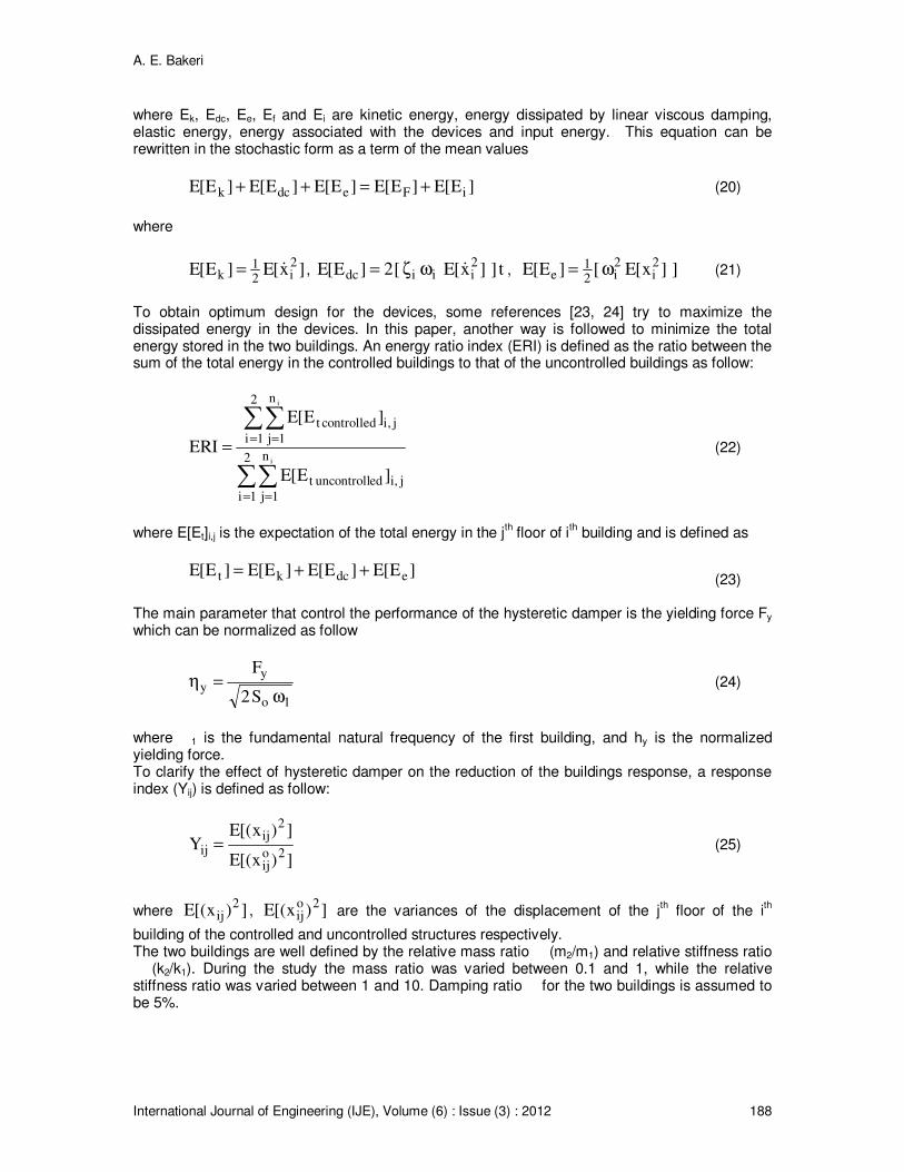
A. E. Bakeri
International Journal of Engineering (IJE), Volume (6) : Issue (3) : 2012 188
where Ek, Edc, Ee, Ef and Ei are kinetic energy, energy dissipated by linear viscous damping, elastic energy, energy associated with the devices and input energy. This equation can be rewritten in the stochastic form as a term of the mean values
]E[E]E[E]E[E]E[E]E[E iFedck +=++ (20)
where
]x[E]E[E2i2
1k &= , t]]x[E[2]E[E
2iiidc &ωζ= , ]]x[E[]E[E
2i
2i2
1e ω= (21)
To obtain optimum design for the devices, some references [23, 24] try to maximize the dissipated energy in the devices. In this paper, another way is followed to minimize the total energy stored in the two buildings. An energy ratio index (ERI) is defined as the ratio between the sum of the total energy in the controlled buildings to that of the uncontrolled buildings as follow:
∑∑
∑∑
= =
= ==
2
1i
n
1j
j,ieduncontrollt
2
1i
n
1j
j,icontrolledt
i
i
]E[E
]E[E
ERI (22)
where E[Et]i,j is the expectation of the total energy in the j
th floor of i
th building and is defined as
]E[E]E[E]E[E]E[E edckt ++= (23)
The main parameter that control the performance of the hysteretic damper is the yielding force Fy which can be normalized as follow
1o
yy
S2
F
ω=η (24)
where �1 is the fundamental natural frequency of the first building, and hy is the normalized yielding force. To clarify the effect of hysteretic damper on the reduction of the buildings response, a response index (Yij) is defined as follow:
])x[(E
])x[(EY
2oij
2ij
ij = (25)
where ])x[(E2
ij , ])x[(E2o
ij are the variances of the displacement of the jth floor of the i
th
building of the controlled and uncontrolled structures respectively. The two buildings are well defined by the relative mass ratio � (m2/m1) and relative stiffness ratio � (k2/k1). During the study the mass ratio was varied between 0.1 and 1, while the relative stiffness ratio was varied between 1 and 10. Damping ratio � for the two buildings is assumed to be 5%.

A. E. Bakeri
International Journal of Engineering (IJE), Volume (6) : Issue (3) : 2012 189
3. RESULTS AND DISCUSSION During this research three different models were developed. The first model consisted of two multi-story adjacent buildings each of them have three stories. The second model consisted of two ten-stories buildings connected with dampers. The third model consisted of ten-story building adjacent to twenty-story building. The details of each model and the main findings are presented in the following sections.
3.1 The First Model Two multi-story adjacent buildings each of them have three stories are analyzed when a hysteretic dampers are provided in each story when the mass and stiffness ratios take the values (�=1, � = 2). The response index of each floor in the two buildings and the ERI are shown in Fig. (2) for different values of damper normalized yielding force (ηy). The figure shows three stages of the dampers. The first stage when no damper is provided (ηy=0). For this stage the response indices and ERI are unit. The second stage when the dampers dissipated energy efficiently (0 < ηy < 100) and in this stage the change of �y changes the response indices and ERI. The third stage when the dampers are worked linearly (100 < ηy) and in this stage the change of ηy changes slightly the response indices and ERI. The obtained results agree with that obtained previously by Basili and De Angelis [23] when they analyzed two single story buildings connected with dampers.
10-1
100
101
102
103
104
0.2
0.3
0.4
0.5
0.6
0.7
0.8
0.9
1
ηy
Y11
Y12
Y13
Y21
Y22
Y23
ERI
FIGURE 2: ERI and response indices versus �y for first model (� = 1, � = 2, �s = 5%)
It is found that there is a minimum value of ERI at (ηy = 1.26). It is also found that the response index for each floor in the two buildings under unit, i.e. the connected dampers reduce the response of all floors, and this reduction is maximum at the point of minimum energy. The response indices of the first building (softer) are smaller than that of the second building (stiffer) because the dominator of the response index is the variance of the uncontrolled buildings which is smaller in the second building than that of the first one. Some references that dealt with two SDOF adjacent buildings [23] stated that this result is not always true especially when there is high difference between the properties of the two buildings as (�=0.1, � = 5) as shown in Fig. (3a). This figure shows the response indices of the second building which are dramatically increased. But this is not true note because when the figure is expanded, the same figure is found as shown in Fig. (3b) but the response indices of the second building skip the unit and reach to 35 for the linear damper. This is not because the response variance of the second controlled building is increased strong but because the second building is very stiff, then the variance of the uncontrolled (ηy=0) is very small as shown in Fig. (3c).

A. E. Bakeri
International Journal of Engineering (IJE), Volume (6) : Issue (3) : 2012 190
10-1
100
101
102
103
104
0
0.2
0.4
0.6
0.8
1
1.2
1.4
1.6
1.8
2
ηy
Y11
Y12
Y13
Y21
Y22
Y23
ERI
FIGURE 3a : Part of ERI and response indices versus �y for first model (� = 0.1, � = 5, �s = 5%)
10-1
100
101
102
103
104
10-2
10-1
100
101
102
ηy
Y11
Y12
Y13
Y21
Y22
Y23
ERI
FIGURE 3b : Complete ERI and response indices versus �y for first model (� = 0.1, � = 5, �s = 5%)

A. E. Bakeri
International Journal of Engineering (IJE), Volume (6) : Issue (3) : 2012 191
10-1
100
101
102
103
104
0
2
4
6
8
10
12
14
ηy
( E
[x2] S
o /
ω3 )
0.5
x11
x12
x13
x21
x22
x23
FIGURE 3c : Response indices versus �y for first model (� = 0.1, � = 5, �s = 5%)
The previous results for a specific properties of the two buildings (� = 1, � = 2). A huge study is performed for wide ranges of the buildings properties to conclude the point the minimum ERI and the corresponding optimum ηy as shown in figures (4, 5). It is noted that the minimum ERI is smaller than the unit in all cases, i.e. there is a dissipation of the energy at this optimum point, and the optimum ηy fluctuates round the unit. The expectation of the response indices of the first and second buildings at the optimum point is shown in figures (6,7) respectively. It is found that the response indices expectation is under until except the second building when become very stiffer (� < 0.17).
0.400330.40033 0.40033
0.42735 0.42735 0.427350.4
5438
0.45438
0.454380.45438
0.4
814
0.48
14 0.4814
0.4814
0.5
0843
0.50843
0.5
35450.5
62
480.5
895
λ
µ
1 2 3 4 5 6 7 8 9 100.1
0.2
0.3
0.4
0.5
0.6
0.7
0.8
0.9
1
FIGURE 4: Minimum values of ERI for different values of ��

A. E. Bakeri
International Journal of Engineering (IJE), Volume (6) : Issue (3) : 2012 192
0.8
822
20.8
8222
0.9
444
40.9
444
4
1.0
06
7
1.0
06
7
1.0
689
1.0
689
1. 0
689
1.0
68
9
1.1
311
1.1
311
1.1
311
1.1
933
1.1
933
1.1933
1.2556
1.2556
1.2556
1.3178
1.3178
λ
µ
1 2 3 4 5 6 7 8 9 100.1
0.2
0.3
0.4
0.5
0.6
0.7
0.8
0.9
1
FIGURE 5: Optimum values of �y for different values of ��
0.1
693
0.1
693
0.1
693
0.2
1487
0.2
1487
0.2
1487
0.2
6045
0.2
6045
0.3
0603
0.3
0603
0.3
516
0.3
9718
0.4
4275
λ
µ
1 2 3 4 5 6 7 8 9 100.1
0.2
0.3
0.4
0.5
0.6
0.7
0.8
0.9
1
FIGURE 6: Expectation of response index of the first building at Optimum �y
0.5
3586
0.5
3586
0.535860.53586
0.53586
0.69384 0.69384 0.69384
0.85183 0.85183 0.851831.0098 1.0098 1.00981.1678 1.1678 1.16781.3258 1.3258 1.32581.48381.48381.4838 1.6418
λ
µ
1 2 3 4 5 6 7 8 9 100.1
0.2
0.3
0.4
0.5
0.6
0.7
0.8
0.9
1
FIGURE 7: Expectation of response index of the second building at Optimum �y

A. E. Bakeri
International Journal of Engineering (IJE), Volume (6) : Issue (3) : 2012 193
3.2 Effect of Damper Stiffness Ratio (�c) The previous work is concerned on the dampers that have a stiffness equals to that of the first buildings (�c=1). When the damper stiffness ratio is changed and ERI is obtained for many cases of buildings properties as shown in Fig. (8). It is shown that after a unit damper stiffness ratio, the variation of the ERI is slight, i.e. the increase of the dampers stiffness does not affect clearly the energy dissipation.
0 1 2 3 4 5 6 7 8 9 100.2
0.4
0.6
0.8
1
1.2
1.4
γc
ER
I
λ=1 µ=1
λ=1 µ=2
λ=1 µ=5
λ=2 µ=1
λ=2 µ=2
λ=2 µ=5
λ=5 µ=1
λ=5 µ=2
λ=5 µ=5
FIGURE 8: ERI of the first model against �c
3.3 Second Model The second model consisted of two ten-stories buildings connected with dampers is analyzed for specific properties (� = 2, � = 1). The normalized damper yield force is changed, and the ERI for the two buildings is calculated and plotted as shown in Fig. (9). The extreme left point close to unit when ηy =0 indicates no damper installed, the extreme right point indicates linear rigid damper, and between them the ERI is varied with the change of ηy and have optimum value at ηy =1. The normalized variances of the two buildings are shown in figures (10 a,b) for the three mentioned cases. The two figures show the normalized variances of the uncontrolled structures, structures connected with elastic rigid damper, and the structures connected with optimum hysteretic damper. It is clear that the optimum hysteretic dampers dissipate the energy and reduce the response of the two buildings. For adjacent buildings with varied relative properties, Fig. (11) shows the minimum values of ERI. It is shown that all values of ERI is less than unit which indicates that the hysteretic dampers reduce the energy in the adjacent buildings in all cases, and its efficiency is pronounced when there is a clear difference between the properties of the two buildings (the lower right corner point). When the two adjacent buildings are similar (� = 1, � = 1, i.e. the upper left corner), the dampers don’t work efficiently. The optimum normalized damper yielding force is around the unit as shown in Fig. (12). The expectation of response indices of the two building at Optimum ηy are shown in figures (13, 14) for varied values of system properties. It is shown that the response of the first building (softer) is less than unit specially when there is high difference between the two buildings (lower right point), while the response of the second building (stiffer) is less than unit until the mass ratio have a value 0.3. Above this value of mass ratio, the hysteretic dampers dissipate the energy and the response of the two buildings are reduces, while under this ratio, the mass of the second building is very light and then the response of the original second building that compared with it is very small. The change of the damper stiffness ratio (�c) affects sharply before the unit and then the change will be slight as shown in Fig. (15) which coincide with that concluded for the first model.

A. E. Bakeri
International Journal of Engineering (IJE), Volume (6) : Issue (3) : 2012 194
10-1
100
101
102
103
104
0.4
0.5
0.6
0.7
0.8
0.9
1
ηy
ER
I
FIGURE 9: ERI of the second model against �y (� = 1, � = 2, �s = 5%)
0 20 40 600
1
2
3
4
5
6
7
8
9
10
( E[x2] So /ω
3 )0.5
Flo
or
Uncontrolled
ERD
Opt. Damper
0 10 20 300
1
2
3
4
5
6
7
8
9
10
( E[x2] S
o /ω
3 )
0.5
Flo
or
Uncontrolled
ERD
Opt. Damper
FIGURE 10: Normalized variance of the two buildings in the second mdoel

A. E. Bakeri
International Journal of Engineering (IJE), Volume (6) : Issue (3) : 2012 195
0.386320.38632 0.38632
0.41446
0.41446 0.41446
0.4
4261
0.44261 0.44261 0.44261
0.4
7075
0.470750.47075
0.47075
0.4
989
0.4
989
0.4989
0.5
2704
0.5
5519
0.5
8333
λ
µ
1 2 3 4 5 6 7 8 9 100.1
0.2
0.3
0.4
0.5
0.6
0.7
0.8
0.9
1
FIGURE 11: Minimum values of ERI of the second model for different values of ��
0.7
7556
0.8
3111
0.8
3111
0. 8
8667
0.8
8667
0.9
4222
0.9
4222
0.9
9778
0.9
9778
0.99778
1.0533
1.0
533
1.05331.1089
1.1089
1.1089
1.1
644
1.1644
λ
µ
1 2 3 4 5 6 7 8 9 100.1
0.2
0.3
0.4
0.5
0.6
0.7
0.8
0.9
1
FIGURE 12: Optimum values of �y for different values of ��
0.1
0421
0.1
0421
0.1
0421
0.1
5532
0.1
5532
0.1
5532
0.2
0644
0.2
0644
0.2
5755
0.2
5755
0.3
0867
0.3
597
90.4
109
λ
µ
1 2 3 4 5 6 7 8 9 100.1
0.2
0.3
0.4
0.5
0.6
0.7
0.8
0.9
1
FIGURE 13: Expectation of response index of the first building at Optimum �y
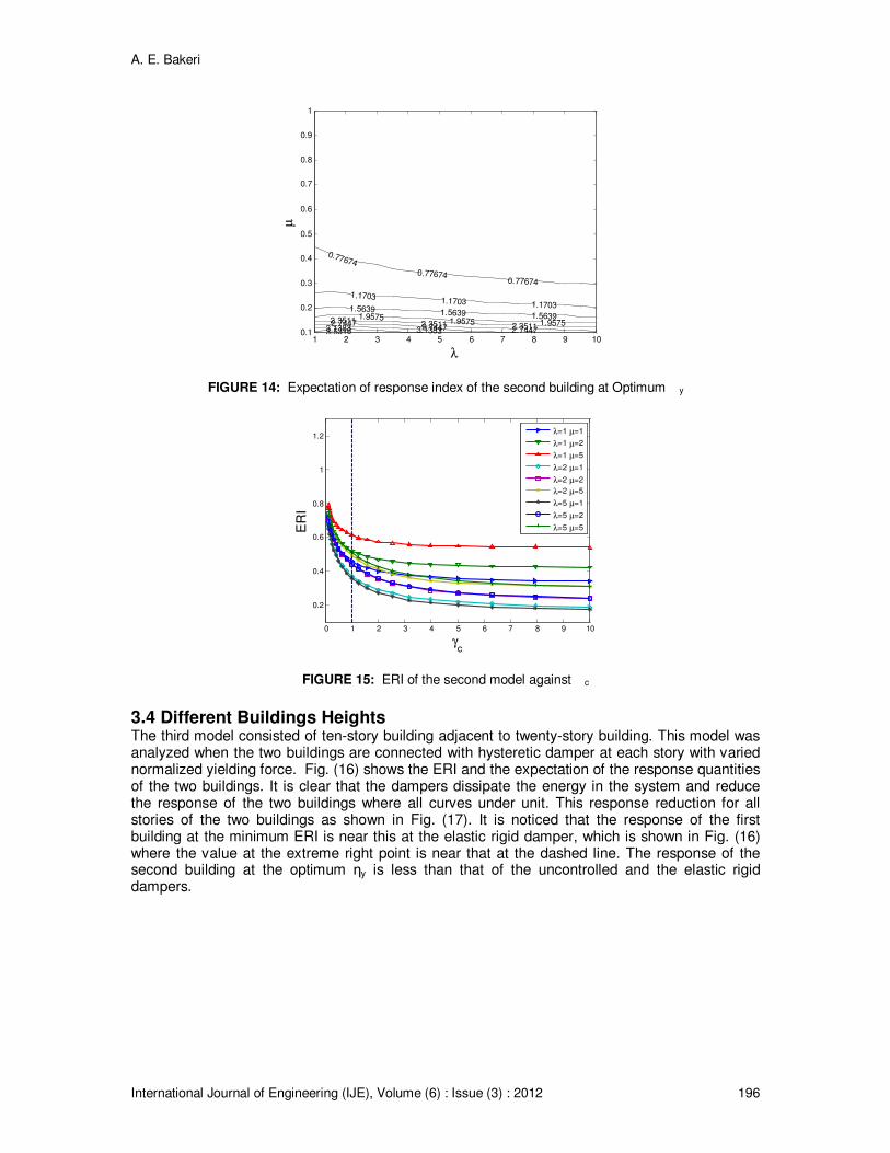
A. E. Bakeri
International Journal of Engineering (IJE), Volume (6) : Issue (3) : 2012 196
0.77674
0.776740.77674
1.1703 1.1703 1.17031.5639 1.5639 1.56391.9575 1.9575 1.95752.3511 2.3511 2.35112.7447 2.7447 2.74473.13833.13833.5318
λ
µ
1 2 3 4 5 6 7 8 9 100.1
0.2
0.3
0.4
0.5
0.6
0.7
0.8
0.9
1
FIGURE 14: Expectation of response index of the second building at Optimum �y
0 1 2 3 4 5 6 7 8 9 10
0.2
0.4
0.6
0.8
1
1.2
γc
ER
I
λ=1 µ=1
λ=1 µ=2
λ=1 µ=5
λ=2 µ=1
λ=2 µ=2
λ=2 µ=5
λ=5 µ=1
λ=5 µ=2
λ=5 µ=5
FIGURE 15: ERI of the second model against �c
3.4 Different Buildings Heights The third model consisted of ten-story building adjacent to twenty-story building. This model was analyzed when the two buildings are connected with hysteretic damper at each story with varied normalized yielding force. Fig. (16) shows the ERI and the expectation of the response quantities of the two buildings. It is clear that the dampers dissipate the energy in the system and reduce the response of the two buildings where all curves under unit. This response reduction for all stories of the two buildings as shown in Fig. (17). It is noticed that the response of the first building at the minimum ERI is near this at the elastic rigid damper, which is shown in Fig. (16) where the value at the extreme right point is near that at the dashed line. The response of the second building at the optimum ηy is less than that of the uncontrolled and the elastic rigid dampers.
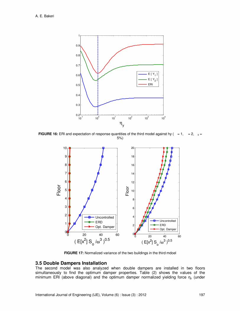
A. E. Bakeri
International Journal of Engineering (IJE), Volume (6) : Issue (3) : 2012 197
10-1
100
101
102
103
104
0.2
0.3
0.4
0.5
0.6
0.7
0.8
0.9
1
ηy
E [ Y1 ]
E [ Y2 ]
ERI
FIGURE 16: ERI and expectation of response quantities of the third model against hy (� = 1, � = 2, �s = 5%)
0 20 40 600
1
2
3
4
5
6
7
8
9
10
( E[x2] S
o /ω
3 )
0.5
Flo
or
Uncontrolled
ERD
Opt. Damper
0 20 40 600
2
4
6
8
10
12
14
16
18
20
( E[x2] So /ω
3 )0.5
Flo
or
Uncontrolled
ERD
Opt. Damper
FIGURE 17: Normalized variance of the two buildings in the third mdoel
3.5 Double Dampers Installation The second model was also analyzed when double dampers are installed in two floors simultaneously to find the optimum damper properties. Table (2) shows the values of the minimum ERI (above diagonal) and the optimum damper normalized yielding force ηy (under

A. E. Bakeri
International Journal of Engineering (IJE), Volume (6) : Issue (3) : 2012 198
diagonal). It is shown that the double dampers dissipate the energy in the two buildings where its values are under unit especially when one of the two dampers is installed at the top floor while the other damper is installed at any floor (the last column in the table). Table (3) shows the expectation of the response indices for the first building (above diagonal) and second one (under diagonal) when double dampers installed. It is clear that the responses of the two buildings are reduced sharply.
1 2 3 4 5 6 7 8 9 10
1 X 0.79 0.75 0.73 0.72 0.72 0.73 0.72 0.72 0.70 2 2.65 X 0.75 0.73 0.71 0.71 0.71 0.71 0.71 0.69 3 2.75 2.40 X 0.72 0.71 0.71 0.71 0.71 0.71 0.70 4 2.70 2.45 2.25 x 0.72 0.71 0.71 0.71 0.71 0.70 5 2.60 2.40 2.25 2.15 X 0.72 0.71 0.71 0.72 0.71
6 2.50 2.40 2.25 2.20 2.10 x 0.73 0.72 0.72 0.71 7 2.25 2.25 2.25 2.15 2.15 1.95 x 0.74 0.73 0.72 8 2.25 2.20 2.10 2.05 2.05 2.00 1.90 x 0.73 0.73 9 2.25 2.20 2.10 2.05 1.95 1.95 1.95 1.85 x 0.73
10 2.35 2.30 2.20 2.15 2.05 2.00 2.00 1.85 1.70 x
TABLE 2: Minimum ERI and optimum �y for Double dampers installed
1 2 3 4 5 6 7 8 9 10
1 X 0.55 0.44 0.37 0.34 0.33 0.33 0.32 0.31 0.31 2 0.67 x 0.42 0.36 0.33 0.31 0.31 0.30 0.30 0.30 3 0.56 0.54 X 0.35 0.32 0.31 0.30 0.30 0.29 0.29
4 0.50 0.49 0.48 x 0.32 0.30 0.30 0.30 0.30 0.29 5 0.47 0.47 0.47 0.47 X 0.31 0.30 0.30 0.30 0.30 6 0.47 0.46 0.47 0.47 0.49 x 0.32 0.31 0.30 0.30 7 0.48 0.48 0.48 0.48 0.50 0.51 x 0.32 0.31 0.31 8 0.48 0.48 0.48 0.49 0.50 0.51 0.52 x 0.32 0.31
9 0.47 0.47 0.48 0.49 0.50 0.51 0.52 0.52 x 0.32 10 0.46 0.46 0.47 0.48 0.49 0.51 0.52 0.51 0.50 x
TABLE 3: Expectation of the response indices for the two buildings for Double dampers installed
3.6 Single Damper Installation A single damper is installed alone in each floor of the two adjacent buildings and they are analyzed to obtain the optimum location and properties of this damper. Table(4) shows the minimum ERI of each case, the corresponding optimum damper normalized yielding force and the expectation of the two buildings in each case. It is shown that the best case when the damper is installed at the top floor. Floor 1 2 3 4 5 6 7 8 9 10
ERI 0.90 0.83 0.79 0.78 0.77 0.78 0.79 0.78 0.77 0.76 Zetay 3.30 3.60 3.45 3.25 3.15 2.90 2.50 2.65 2.65 2.65 E(E[x1,i]) 7.81 5.54 4.38 3.81 3.50 3.46 3.60 3.42 3.33 3.35 E(E[x2,i]) 8.57 6.75 5.58 4.97 4.82 4.94 5.03 4.99 4.87 4.79
TABLE 4: Single damper results
4. SUMMARY AND CONCLUSIONS The dynamic behaviour of two adjacent MDOF structures connected with a hysteretic damper was studied to obtain the optimum properties of the connecting dampers when subjected to white-noise random excitation based on the minimization of the stored energy in the entire system. It is concluded that:
1. The connecting dampers reduce the response of the two adjacent structures sharply.
A. E. Bakeri
International Journal of Engineering (IJE), Volume (6) : Issue (3) : 2012 199
2. The benefit of the dampers is pronounced when there is clear difference between the two structures.
3. The optimum damper stiffness is equal to that of the first structure. 4. When two dampers only are installed, it is preferred to install one at of them at the top
floor and the other in any floor. 5. When single damper only are installed, it is preferred to install it at the top floor.
5. REFERENCES [1] Y.L. Xu, Q. He, J.M. Ko, Dynamic response of damper-connected adjacent buildings under
earthquake excitation, Engineering Structures 21 (1999), 135-148.
[2] H.P. Hong, S.S. Wang, P. Hong, Critical building separation distance in reducing pounding risk under earthquake excitation, Structural Safety 25 (2003), 287-303.
[3] S.S. Wang, H.P. Hong, Quantiles of critical separation distance for nonstationary seismic excitations, Engineering Structures 28 (2006), 985-991.
[4] D.L. Garcia, T.T. Soong, Evaluation of current criteria in predicting the separation necessary to prevent seismic pounding between nonlinear hysteretic structural systems, Engineering Structures 31 (2009), 1217-1229.
[5] S.E. Abdel Raheem, Seismic Pounding between Adjacent Building Structures, Electronic Journal of Structural Engineering, 6 (2006), 66-74.
[6] B. Westermo, The dynamics of interstructural connection to prevent pounding, Earthquake Engineering and Structural Dynamics 18 (1989), 687- 699.
[7] T. Kobori, T. Yamada, Y. Takenaka, Effect of dynamic tuned connector on reduction of seismic response application to adjacent office buildings, Proceedings of the Ninth World Conference Earthquake Engineering, Vol. 5, Tokio-Kioto, Japan, (1988), 773-778.
[8] H.P. Zhu, H. Iemura, A study of response control on the passive coupling element between parallel structures, Structural Engineering and Mechanics 9 (2000), 383-396.
[9] WS. Zhang, YL. Xu, Dynamic characteristics and seismic response of adjacent buildings linked by discrete dampers, Earthquake Engineering and Structural Dynamics 28, (1999), 1163-1185.
[10] J. Kima, J. Ryua, L. Chungb, Seismic performance of structures connected by viscoelastic dampers, Engineering Structures 28 (2006), 183-195.
[11] Y.L. Xu, S. Zhan, J.M. Ko and W.S. Zhang, experimental investigation of adjacent buildings connected by fluid damper, Earthquake Engineering and Structural Dynamics 28 (1999), 609-631.
[12] W.S. Zhang and Y.L. Xu, vibration analysis of two buildings linked by maxwell model-defined fluid dampers, Journal of Sound and vibration 233 (2000), 775-796.
[13] S.D. Bharti, S.M. Dumne, M.K. Shrimali , Seismic response analysis of adjacent buildings connected with MR dampers, Engineering Structures 32 (2010), 2122-2133.
[14] A.V. Bhaskararao, R.S. Jangid, Harmonic response of adjacent structures connected with a friction damper, Journal of Sound and Vibration 292 (2006), 710-725.

A. E. Bakeri
International Journal of Engineering (IJE), Volume (6) : Issue (3) : 2012 200
[15] A.V. Bhaskararao, R.S. Jangid, Seismic analysis of structures connected with friction dampers, Engineering Structures 28 (2006), 690-703.
[16] YQ. Ni, JM. Ko, ZG. Ying, Random seismic response analysis of adjacent buildings coupled with non-linear hysteretic dampers. Journal of Sound and Vibration 246 (2001), 403-417.
[17] M.M. Abdullah, J.H. Hanif, A. Richardson and J. Sobanjo, Use of a shared tuned mass damper (STMD) to reduce vibration and pounding in adjacent structures, Earthquake Engineering and Structural Dynamics 30 (2001), 1185-1201.
[18] J.E. Luco, F.C.P. De Barros, Control of the seismic response of a composite tall building modelled by two interconnected shear beams, Earthquake Engineering and Structural Dynamics 27 (1998) 205-223.
[19] T. AIDA AND T. ASO, improvement of the structure damping performance by interconnection, Journal of Sound and vibration 242 (2001), 333-353.
[20] H.P. Zhu, Y.L. Xu, Optimum parameters of Maxwell model-defined dampers used to link adjacent structures, Journal of Sound and Vibration 279 (2005), 253-274.
[21] S.Y. Ok, J. Song, K.S. Park, Optimal design of hysteretic dampers connecting adjacent structures using multi-objective genetic algorithm and stochastic linearization method, Engineering Structures 30 (2008), 1240-1249.
[22] A. V. Bhaskararao and R. S. Jangid, Optimum viscous damper for connecting adjacent SDOF structures for harmonic and stationary white-noise random excitations, Earthquake Engineering and Structural Dynamics 36 (2007), 563-571.
[23] M. Basili, M. De Angelis, Optimal passive control of adjacent structures interconnected with nonlinear hysteretic devices, Journal of Sound and Vibration 301 (2007), 106-125.
[24] M. Basili, M. De Angelis, A reduced order model for optimal design of 2-mdof adjacent structures connected by hysteretic dampers, Journal of Sound and Vibration 306 (2007), 297-317.
[25] A.E. Bakeri, Stochastic analysis of base isolated structure, PhD thesis, Faculty of Eng., Zagazig University, 2000.
[26] Y.K. Wen, Method for random vibration of hysteretic systems, Journal of the Engineering Mechanics Division, Proceedings of the American Society of Civil Engineers 102 (1976), 249-263.

INSTRUCTIONS TO CONTRIBUTORS The International Journal of Engineering (IJE) is devoted in assimilating publications that document development and research results within the broad spectrum of subfields in the engineering sciences. The journal intends to disseminate knowledge in the various disciplines of the engineering field from theoretical, practical and analytical research to physical implications and theoretical or quantitative discussion intended for both academic and industrial progress. Our intended audiences comprises of scientists, researchers, mathematicians, practicing engineers, among others working in Engineering and welcome them to exchange and share their expertise in their particular disciplines. We also encourage articles, interdisciplinary in nature. The realm of International Journal of Engineering (IJE) extends, but not limited, to the following: To build its International reputation, we are disseminating the publication information through Google Books, Google Scholar, Directory of Open Access Journals (DOAJ), Open J Gate, ScientificCommons, Docstoc and many more. Our International Editors are working on establishing ISI listing and a good impact factor for IJE. The initial efforts helped to shape the editorial policy and to sharpen the focus of the journal. Starting with volume 6, 2012, IJE appears in more focused issues. Besides normal publications, IJE intend to organized special issues on more focused topics. Each special issue will have a designated editor (editors) – either member of the editorial board or another recognized specialist in the respective field. We are open to contributions, proposals for any topic as well as for editors and reviewers. We understand that it is through the effort of volunteers that CSC Journals continues to grow and flourish.
IJE LIST OF TOPICS The realm of International Journal of Engineering (IJE) extends, but not limited, to the following:
• Aerospace Engineering • Agricultural Engineering
• Biomedical Engineering • Chemical Engineering
• Civil & Structural Engineering • Computer Engineering
• Control Systems Engineering • Education Engineering
• Electrical Engineering • Electronic Engineering
• Engineering Mathematics • Engineering Science
• Environmental Engineering • Fluid Engineering
• Geotechnical Engineering • Industrial Engineering
• Manufacturing Engineering • Materials & Technology Engineering
• Mechanical Engineering • Mineral & Mining Engineering
• Nuclear Engineering • Optical Engineering
• Petroleum Engineering • Robotics & Automation Engineering
• Telecommunications Engineering
CALL FOR PAPERS Volume: 6 - Issue: 5 - October 2012 i. Paper Submission: July 31, 2012 ii. Author Notification: September 15, 2012
iii. Issue Publication: October 2012

CONTACT INFORMATION
Computer Science Journals Sdn BhD
B-5-8 Plaza Mont Kiara, Mont Kiara 50480, Kuala Lumpur, MALAYSIA
Phone: 006 03 6207 1607
006 03 2782 6991
Fax: 006 03 6207 1697
Email: [email protected]