international journal of approximate reasoninglzhang/paper/pspdf/poon-zhang-ijar-2013.pdf ·...

International Journal of Approximate Reasoning 54 (2013) 196–215

Contents lists available at SciVerse ScienceDirect

International Journal of Approximate Reasoning

j o u r n a l h o m e p a g e : w w w . e l s e v i e r . c o m / l o c a t e / i j a r

Model-based clustering of high-dimensional data: Variable selection versus

facet determination<

Leonard K.M. Poon ∗, Nevin L. Zhang, Tengfei Liu, April H. Liu

Department of Computer Science and Engineering, The Hong Kong University of Science and Technology, Hong Kong, China

A R T I C L E I N F O A B S T R A C T

Article history:

Received 8 July 2011

Received in revised form 18 July 2012

Accepted 6 August 2012

Available online 16 August 2012

Keywords:

Model-based clustering

Facet determination

Variable selection

Latent tree models

Gaussian mixture models

Variable selection is an important problem for cluster analysis of high-dimensional data. It

is also a difficult one. The difficulty originates not only from the lack of class information

but also the fact that high-dimensional data are oftenmultifaceted and can bemeaningfully

clustered in multiple ways. In such a case the effort to find one subset of attributes that

presumably gives the “best” clustering may be misguided. It makes more sense to identify

various facets of a data set (each being based on a subset of attributes), cluster the data

along each one, and present the results to the domain experts for appraisal and selection. In

this paper, we propose a generalization of the Gaussianmixturemodels and demonstrate its

ability to automatically identify natural facets of data and cluster data along each of those

facets simultaneously.Wepresent empirical results to show that facet determinationusually

leads to better clustering results than variable selection.

© 2012 Elsevier Inc. All rights reserved.

1. Introduction

Variable selection is an important issue for cluster analysis of high-dimensional data. The cluster structure of interest

to domain experts can often be best described using a subset of attributes. The inclusion of other attributes can degrade

clustering performance and complicate cluster interpretation. Recently there is a growing interest in the issue [2–4]. This

paper is concerned with variable selection for model-based clustering.

In classification, variable selection is a clearly defined problem, i.e., to find the subset of attributes that gives the best

classification performance. The problem is less clear for cluster analysis due to the lack of class information. Severalmethods

have been proposed for model-based clustering. Most of them introduce flexibility into the generative mixture model to

allow clusters to be related to subsets of (instead of all) attributes and determine the subsets alongside parameter estimation

or during a separatemodel selection phase. Raftery and Dean [5] consider a variation of the Gaussianmixturemodel (GMM)

where the latent variable is related to a subset of attributes and is independent of other attributes given the subset. A greedy

algorithm is proposed to search among thosemodels for onewith high BIC score. At each search step, two nestedmodels are

compared using the Bayes factor and the better one is chosen to seed the next search step. Law et al. [6] start with the Naïve

Bayes model (i.e., GMMwith diagonal covariance matrices) and add a saliency parameter for each attribute. The parameter

ranges between 0 and 1. When it is 1, the attribute depends on the latent variable. When it is 0, the attribute is independent

of the latent variable and its distribution is assumed to be unimodal. The saliency parameters are estimated together with

other model parameters using the EM algorithm. The work is extended by Li et al. [7] so that the saliency of an attribute can

vary across clusters. The third line of work is based on GMMswhere all clusters share a common diagonal covariancematrix,

while their meansmay vary. If themean of a cluster along an attribute turns out to coincide with the overall mean, then that

attribute is irrelevant to cluster. Both Bayesian methods [8,9] and regularization methods [10] have been developed based

on this idea.

< An earlier version of this paper appears in [1].∗ Corresponding author.

E-mail addresses: [email protected] (L.K.M. Poon), [email protected] (N.L. Zhang), [email protected] (T. Liu), [email protected] (A.H. Liu).

0888-613X/$ - see front matter © 2012 Elsevier Inc. All rights reserved.

http://dx.doi.org/10.1016/j.ijar.2012.08.001


http://www.sciencedirect.com/science/journal/0888613X

www.elsevier.com/locate/ijar


L.K.M. Poon et al. / International Journal of Approximate Reasoning 54 (2013) 196–215 197

Our work is based on two observations. First, while clustering algorithms identify clusters in data based on the charac-

teristics of data, domain experts are ultimately the ones to judge the interestingness of the clusters found. Second, high-

dimensional data are oftenmultifaceted in the sense that theremay bemultiplemeaningful ways to partition them. The first

observation is the reason why variable selection for clustering is such a difficult problem, whereas the second one suggests

that the problem may be ill-conceived from the start.

Instead of the variable selection approach, we advocate a facet determination approach. The idea is to systematically

identify all the different facets of a data set, cluster the data along each one, and present the results to the domain experts

for appraisal and selection. The analysis would be useful if one of the clusterings is found interesting.

The difference between the two approaches can be elucidated by comparing their objectives. In variable selection, the

aim is to find one subset of attributes that gives the “best” or “good” clustering result. In facet determination, the aim is to

findmultiple subsets of attributes such that each subset gives meaningful partition of data. In other words, performing facet

determination can be considered as performing multiple variable selection simultaneously, without assuming that there is

only a single “best” solution.

To realize the idea of facet determination, we generalize the GMMs to allowmultiple latent variables. For computational

tractability, we restrict that each attribute can be connected to only one latent variable and the relationships among the

latent variables can be represented as a tree. The result is what we call pouch latent tree models (PLTMs). Analyzing data

using a PLTMmay result in multiple latent variables. Each latent variable represents a partition (clustering) of the data and

is usually related primarily to only a subset of attributes. Consequently, facets of data can be identified by those subsets of

attributes.

Facet determination has been investigated under different designations in previous work. Two other classes of models

have been considered. Galimberti and Soffritti [11] use a collection of GMMs, each on a disjoint subset of attributes, for facet

determination. We refer to their method as the GS method. The method starts by obtaining a partition of attributes using

variable clustering. A GMM is built on each subset of attributes and the collection of GMMs is evaluated using the BIC score.

To look for the optimal partition of attributes, the method repeatedly merges the two subsets of attributes that lead to the

largest improvement in the BIC score. It stopswhen no subsets can bemerged to improve the score. Similar to the GSmodels,

PLTMs can be considered as containing a collection of GMMs on disjoint subsets of attributes. However, the GMMs in PLTMs

are connected by a tree structure, whereas those in the GS models are disconnected.

Latent treemodels (LTMs) [12,13] are another class of models that have been used for facet determination [14]. LTMs and

PLTMs are much alike. However, LTMs include only discrete variables and can handle only discrete data. PLTMs generalize

LTMs by allowing continuous variables. As a result, PLTMs can also handle continuous data.

Two contributions are made in this paper. The first one is a new class of models in PLTMs, resulting from the marriage

between GMMs and LTMs. PLTMs not only generalize GMMs to allowmultiple latent variables, but they also generalize LTMs

for handling continuous data. The generalization of LTMs is interesting for two reasons. First, it is desirable to have a tool for

facet determination on continuous data. Second, the generalization is technically non-trivial. It requires new algorithms for

inference and structural learning.

The second contribution is that we compare the variable selection approach and the facet determination approach for

model-based clustering. The two approaches have not been compared in the previous studies on facet determination [11,14].

In this paper, we show that facet determination usually leads to better clustering results than variable selection.

The rest of the paper is organized as follows. Section 2 reviews traditional model-based clustering using GMMs. PLTMs

is then introduced in Section 3. In Sections 4–6, we discuss inference, estimation, and structural learning for PLTMs. The

empirical evaluation is divided into two parts. In Section 7, we analyze real-world basketball data using PLTMs. We aim to

demonstrate the effectiveness of using PLTMs for facet determination. In Section 8, we compare PLTMs with other methods

on benchmark data. We aim to compare the facet determination approach and the variable selection approach. After the

empirical evaluation, we discuss related work in Section 9 and conclude in Section 10.

2. Background and notations

In this paper, we use capital letters such as X and Y to denote random variables, lower case letters such as x and y to

denote their values, and bold face letters such as X , Y , x, and y to denote sets of variables or values.

Finite mixture models are commonly used in model-based clustering [15,16]. In finite mixture modeling, the population

is assumed to bemade up from a finite number of clusters. Suppose a variable Y is used to indicate this cluster, and variables

X represent the attributes in the data. The variable Y is referred to as a latent (or unobserved) variable, and the variables X

asmanifest (or observed) variables. The manifest variables X is assumed to follow a mixture distribution

P(x) =∑y

P(y)P(x|y).

The probability values of the distribution P(y) are known asmixing proportions and the conditional distributions P(x|y) areknown as component distributions. To generate a sample, the model first picks a cluster y according to the distribution P(y)and then uses the corresponding component distribution P(x|y) to generate values for the observed variables.

198 L.K.M. Poon et al. / International Journal of Approximate Reasoning 54 (2013) 196–215

Fig. 1. (a) An example of PLTM. The latent variables are shown in shaded nodes. The numbers in parentheses show the cardinalities of the discrete variables. (b)

Generative model for synthetic data. (c) GMM as a special case of PLTM.

Gaussian distributions are often used as the component distributions due to computational convenience. A Gaussian

mixture model (GMM) has a distribution given by

P(x) =∑y

P(y)N(x|μy,�y),

where N(x|μy,�y) is a multivariate Gaussian distribution, with mean vector μy and covariance matrix �y conditional on

the value of Y .

The Expectation-Maximization (EM) algorithm [17] can be used to fit the model. Once the model is fit, the probability

that a data point d belongs to cluster y can be computed by

P(y|d) ∝ P(y)N(d|μy,�y),

where the symbol ∝ implies that the exact values of the distribution P(y|d) can be obtained by using the sum∑y P(y)N(d|μy,�y) as a normalization constant.

The number G of components (or clusters) can be givenmanually or determined bymodel selection automatically. In the

latter case, a score is used to evaluate a model with G clusters. The G that leads to the highest score is then chosen as the

estimated number of components. The BIC score has been empirically shown to perform well for this purpose [18].

3. Pouch latent tree models

A pouch latent treemodel (PLTM) is a rooted tree, where each internal node represents a latent variable, and each leaf node

represents a set of manifest variables. All the latent variables are discrete, while all the manifest variables are continuous. A

leaf node may contain a single manifest variable or several of them. Because of the second possibility, leaf nodes are called

pouch nodes. 1 Fig. 1a shows an example of PLTM. In this example, Y1–Y4 are discrete latent variables, where Y1–Y3 have three

possible values and Y4 has two. X1–X9 are continuous manifest variables. They are grouped into five pouch nodes, {X1, X2},{X3}, {X4, X5}, {X6}, and {X7, X8, X9}.Beforewemove on, we need to explain some other notations.We use capital letter�(V) to indicate the parent variable of

a variable V and lower case letter π(V) to denote its value. Also, we reserve the use of bold capital letterW for denoting the

variables of a pouch node. When the meaning is clear from context, we use the terms ‘variable’ and ‘node’ interchangeably.

In a PLTM, the dependency of a discrete latent variable Y on its parent �(Y) is characterized by a conditional discrete

distribution P(y|π(Y)). 2 Let W be the variables of a pouch node with a parent node Y = �(W). We assume that, given a

value y of Y ,W follows the conditional Gaussian distribution P(w|y) = N(w|μy,�y)with mean vector μy and covariance

matrix�y. A PLTM can bewritten as a pairM = (m, θ), wherem denotes themodel structure and θ denotes the parameters.

Example 1. Fig. 1b gives another example of PLTM. In this model, there are two discrete latent variables Y1 and Y2, each

having three possible values {s1, s2, s3}. There are six pouch nodes, namely {X1, X2}, {X3}, {X4}, {X5}, {X6}, and {X7, X8, X9}.The variables in the pouch nodes are continuous.

Each node in the model is associated with a distribution. The discrete distributions P(y1) and P(y2|y1), associated with

the two discrete nodes, are given in Table 1.

The pouch nodes W are associated with conditional Gaussian distributions. These distributions have parameters for

specifying the conditional meansμπ(W) and conditional covariances�π(W). For the four pouch nodes with single variables,

{X3}, {X4}, {X5}, and {X6}, these parameters have scalar values. The conditional meanμy for each of these variables is either

−2.5, 0 or 2.5, depending onwhether y = s1, s2, or s3, where y is the value of the corresponding parent variable Y ∈ {Y1, Y2}.1 In fact, PLTMs allow both discrete and continuousmanifest variables. The leaf nodesmay contain either a single discrete variable, a single continuous variable,

or multiple continuous variables. For brevity, we focus on continuous manifest variables in this paper.2 The root node is regarded as the child of a dummy node with only one value, and hence is treated in the same way as other latent nodes.


Table 1

Discrete distributions in Example 1.

y1 P(y1)

s1 0.33s2 0.33s3 0.34

y2 P(y2|y1)y1 = s1 y1 = s2 y1 = s3

s1 0.74 0.13 0.13s2 0.13 0.74 0.13s3 0.13 0.13 0.74

The conditional covariances �y can also have different values for different values of their parents. However, for simplicity

in this example, we set�y = 1,∀y ∈ {s1, s2, s3}.Let p be the number of variables in a pouch node. The conditional means are specified by p-vectors and the conditional

covariances by p× pmatrices. For example, the conditional means and covariances of the pouch node {X1, X2} are given by:

μy1=

⎧⎪⎨⎪⎩

(−2.5,−2.5) : y1 = s1

(0, 0) : y1 = s2

(2.5, 2.5) : y1 = s3

and �y1 =⎛⎝ 1 0.5

0.5 1

⎞⎠ , ∀y1 ∈ {s1, s2, s3}.

The conditional means and covariances are specified similarly for pouch node {X7, X8, X9}. The conditional means for Xi, i ∈{7, 8, 9}, can be −2.5, 0, or 2.5. The variance of any of these variables is 1, and the covariance between any pair of thesevariables is 0.5. �

PLTMs have a noteworthy two-way relationship with GMMs. On the one hand, PLTMs generalize the structure of GMMs

to allow more than one latent variable in a model. Thus, a GMM can be considered as a PLTM with only one latent variable

and one pouch node containing all manifest variables. As an example, a GMM is depicted as a PLTM in Fig. 1c, in which Y1 is

a discrete latent variable and X1–X9 are continuous manifest variables.

On the other hand, the distribution of a PLTM over the manifest variables can be represented by a GMM. Consider a

PLTM M. Suppose W1, . . . ,Wb are the b pouch nodes and Y1, . . . , Yl are the l latent nodes in M. Denote as X = ⋃bi=1 W i

and Y = {Yj : j = 1, . . . , l} the sets of all manifest variables and all latent variables in M, respectively. The probability

distribution defined by M over the manifest variables X is given by

P(x)=∑y

P(x, y)

=∑y

l∏j=1

P(yj|π(Yj))b∏

i=1N(wi|μπ(W i)

,�π(W i)) (1)

=∑y

P(y)N(x|μy, �y). (2)

Eq. (1) follows from the model definition. Eq. (2) follows from the fact that�(W i),�(Yj) ∈ Y and the product of Gaussian

distributions is also a Gaussian distribution. Eq. (2) shows that P(x) is a mixture of Gaussian distributions. Although it

means that PLTMs are not more expressive than GMMs on the distributions of observed data, PLTMs have two advantages

over GMMs. First, numbers of parameters can be reduced in PLTMs by exploiting the conditional independence between

variables, as expressed by the factorization in Eq. (1). Second, and more important, the multiple latent variables in PLTMs

allow multiple clusterings on data.

Example 2. In this example, we compare the numbers of parameters in a PLTM and in a GMM. Consider a discrete node

and its parent node with c and c′ possible values, respectively. It requires (c− 1)× c′ parameters to specify the conditional

discrete distribution for this node. Consider a pouch node with p variables, and its parent variable with c′ possible values.

This node has p× c′ parameters for the conditional mean vectors andp(p+1)

2× c′ parameters for the conditional covariance

matrices. Now consider the PLTM in Fig. 1a and theGMM in Fig. 1c. Both of themdefine a distribution on 9manifest variables.

Based on the above expressions, the PLTM has 77 parameters and the GMM has 164 parameters.Given the same number of manifest variables, a PLTM may appear to be more complex than a GMM, due to a larger

number of latent variables. However, this example shows that a PLTM can still require fewer parameters than a GMM. �

The graphical structure of PLTMs looks similar to that of the Bayesian networks (BNs) [19]. In fact, a PLTM is different from

a BN only because of the possibility of multiple variables in a single pouch node. It has been shown that any nonsingular

multivariate Gaussian distribution can be converted to a complete Gaussian Bayesian network (GBN) with an equivalent

distribution [20]. Therefore, a pouch node can be considered as a shorthand notation of a complete GBN. If we convert each

pouch node into a complete GBN, a PLTM can be considered as a conditional Gaussian Bayesian network (i.e., a BN with

discrete distributions and conditional Gaussian distributions), or a BN in general.


Cluster analysis based on PLTMs requires learning PLTMs from data. It involves parameter estimation and structure

learning. We discuss the former problem in Section 5, and the two problems as a whole in Section 6. Since parameter

estimation involves inference on the model, we discuss this problem in the next section before the other two problems.

4. Inference

A PLTM defines a probability distribution P(X, Y) over manifest variables X and latent variables Y . Consider observing

values e for the evidence variables E ⊆ X . For a subset of variables Q ⊆ X ∪ Y , we are often required to compute the

posterior probability P(q|e). For example, classifying a data point d to one of the clusters represented by a latent variable Y

requires us to compute P(y|X = d).Inference refers to the computation of the posterior probability P(q|e). It can be done on PLTMs similarly as the clique tree

propagation on conditional GBNs [21]. However, due to the existence of pouch nodes in PLTMs, this propagation algorithm

requires some modifications. The inference algorithm is discussed in details in Appendix A.

The structure of PLTMs allows an efficient inference. Letnbe thenumber of nodes in a PLTM, c be themaximumcardinality

of a discrete variable, and p be the maximum number of variables in a pouch node. The time complexity of the inference

is dominated by the steps related to message passing and incorporation of evidence on continuous variables. The message

passing step requiresO(nc2) time, since each cliquehas atmost twodiscrete variables due to the tree structure. Incorporation

of evidence requires O(ncp3) time.

Suppose we have the same number of manifest variables. Since PLTMs generally has smaller pouch nodes than GMMs,

and hence a smaller p, the term O(ncp3) shows that inference on PTLMs can be faster than that on GMMs. This happens even

though PLTMs can have more nodes and thus a larger n.

5. Parameter estimation

Suppose there is a data set D with N samples d1, . . . , dN . Each sample consists of values for the manifest variables.

Consider computing themaximum likelihood estimate (MLE) θ∗ of the parameters for a given PLTM structurem. We do this

using the EM algorithm. The algorithm starts with an initial estimate θ (0) and improves the estimate iteratively.

Suppose the parameter estimate θ (t−1) is obtained after t−1 iterations. The t-th iteration consists of two steps, an E-step

and aM-step. In the E-step, we compute, for each latent node Y and its parent�(Y), the distributions P(y, π(Y)|dk, θ(t−1))

and P(y|dk, θ(t−1)) for each sample dk . This is done by the inference algorithm discussed in the previous section. For each

sample k, let wk be the values of variables W of a pouch node for the sample dk . In the M-step, the new estimate θ (t) isobtained as follows:

P(y|π(Y), θ (t)) ∝N∑

k=1P(y, π(Y)|dk, θ

(t−1)),

μ(t)y =∑N

k=1 P(y|dk, θ(t−1))wk∑N

k=1 P(y|dk, θ(t−1))

,

�(t)y =∑N

k=1 P(y|dk, θ(t−1))(wk − μ

(t)y )(wk − μ

(t)y )′

∑Nk=1 P(y|dk, θ

(t−1)),

where μ(t)y and �

(t)y here correspond to the distribution P(w|y, θ (t)) for nodeW conditional on its parent Y = �(W). The

EM algorithm proceeds to the (t+ 1)-th iteration unless the improvement of log-likelihood log P(D|θ (t))− log P(D|θ (t−1))falls below a certain threshold.

The starting values of the parameters θ (0) are chosen as follows. For P(y|π(Y), θ (0)), the probabilities are randomly

generated from a uniform distribution over the interval (0, 1] and are then normalized. The initial values of μ(0)y are set to

equal to a random sample from data, while those of �(0)y are set to equal to the sample covariance.

Like in the case of GMMs, the likelihood is unbounded in the case of PLTMs. Thismight lead to spurious localmaxima [15].

For example, consider a mixture component that consists of only one data point. If we set the mean of the component to be

equal to that data point and set the covariance to zero, then the model will have an infinite likelihood on the data. However,

even though the likelihoodof thismodel is higher than someothermodels, it doesnotmean that the corresponding clustering

is better. The infinite likelihood can always be achieved by trivially grouping one of the data points as a cluster. This is why

we refer to this kind of local maxima as spurious.

To mitigate this problem, we use a variant of the method by Ingrassia [22]. In the M-step of EM, we need to compute

the covariance matrix �(t)y for each pouch node W . We impose the following constraints on the eigenvalues λ(t) of �

(t)y :


σ 2min/γ ≤ λ(t) ≤ σ 2

max × γ , where σ 2min and σ 2

max are the minimum and maximum of the sample variances of the variables

W and γ is a parameter for our method.

6. Structure learning

Given a data set D, we aim at finding the model m∗ that maximizes the BIC score [23]:

BIC(m|D) = log P(D|m, θ∗)− d(m)

2log N,

where θ∗ is the MLE of the parameters and d(m) is the number of independent parameters inm. The first term is known as

the likelihood term. It favorsmodels that fit datawell. The second term is known as the penalty term. It discourages complex

models. Hence, the BIC score provides a trade-off between model fit and model parsimoniousness.

We have developed a hill-climbing algorithm to search for m∗. It starts with a model m(0) that contains one latent node

as root and a separate pouch node for each manifest variable as a leaf node. The latent variable at the root node has two

possible values. Suppose a model m(j−1) is obtained after j − 1 iterations. In the j-th iteration, the algorithm uses some

search operators to generate candidatemodels bymodifying the basemodelm(j−1). The BIC score is then computed for each

candidate model. The candidate model m′ with the highest BIC score is compared with the base model m(j−1). If m′ has ahigher BIC score than m(j−1), m′ is used as the new base model m(j) and the algorithm proceeds to the (j + 1)-th iteration.

Otherwise, the algorithm terminates and returns m∗ = m(j−1) (together with the MLE of the parameters).

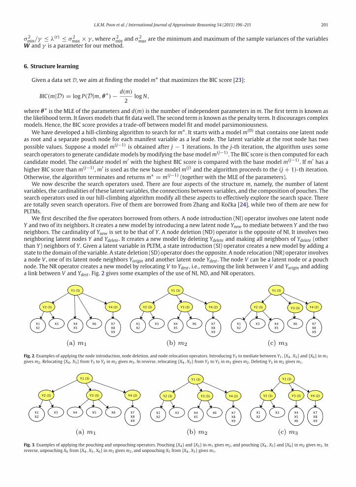
We now describe the search operators used. There are four aspects of the structure m, namely, the number of latent

variables, the cardinalities of these latent variables, the connections between variables, and the composition of pouches. The

search operators used in our hill-climbing algorithm modify all these aspects to effectively explore the search space. There

are totally seven search operators. Five of them are borrowed from Zhang and Kocka [24], while two of them are new for

PLTMs.

We first described the five operators borrowed from others. A node introduction (NI) operator involves one latent node

Y and two of its neighbors. It creates a newmodel by introducing a new latent node Ynew to mediate between Y and the two

neighbors. The cardinality of Ynew is set to be that of Y . A node deletion (ND) operator is the opposite of NI. It involves two

neighboring latent nodes Y and Ydelete. It creates a new model by deleting Ydelete and making all neighbors of Ydelete (other

than Y) neighbors of Y . Given a latent variable in PLTM, a state introduction (SI) operator creates a new model by adding a

state to the domain of the variable. A state deletion (SD) operator does the opposite. A node relocation (NR) operator involves

a node V , one of its latent node neighbors Yorigin and another latent node Ydest . The node V can be a latent node or a pouch

node. The NR operator creates a newmodel by relocating V to Ydest , i.e., removing the link between V and Yorigin and adding

a link between V and Ydest . Fig. 2 gives some examples of the use of NI, ND, and NR operators.

Fig. 2. Examples of applying the node introduction, node deletion, and node relocation operators. Introducing Y3 to mediate between Y1, {X4, X5} and {X6} inm1

givesm2. Relocating {X4, X5} from Y3 to Y2 inm2 givesm3. In reverse, relocating {X4, X5} from Y2 to Y3 inm3 givesm2. Deleting Y3 inm2 givesm1.

Fig. 3. Examples of applying the pouching and unpouching operators. Pouching {X4} and {X5} inm1 givesm2, and pouching {X4, X5} and {X6} inm2 givesm3. In

reverse, unpouching X6 from {X4, X5, X6} inm3 givesm2, and unpouching X5 from {X4, X5} givesm1.


Fig. 4. PLTM obtained on NBA data. The latent variables represent different clusterings on the players. They have been renamed based on our interpretation of

their meanings. The abbreviations in these names stand for: role (Role), general ability (Gen), technical fouls (T), disqualification (D), tall-player ability (Tall),

shooting accuracy (Acc), and three-pointer ability (3pt).

The two new operators are pouching (PO) and unpouching (UP) operators. The PO operator creates a new model by

combining a pair of sibling pouch nodesW1 andW2 into a newpouch nodeWpo = W1∪W2. The UP operator creates a new

model by separating one manifest variable X from a pouch nodeWup, resulting in two sibling pouch nodesW1 = Wup\{X}and W2 = {X}. Fig. 3 shows some examples of the use of these two operators.

The purpose of the PO and UP operators is to modify the conditional independencies entailed by the model on the

variables of the pouch nodes. For example, consider the two models m1 and m2 in Fig. 3. In m1, X4 and X5 are conditionally

independent given Y3, i.e., P(X4, X5|Y3) = P(X4|Y3)P(X5|Y3). In other words, covariance between X4 and X5 is zero given

Y3. On the other hand, X4 and X5 need not be conditionally independent given Y3 inm2. The covariances between them are

allowed to be non-zero in the 2× 2 conditional covariance matrices for the pouch node {X4, X5}.The PO operator in effect postulates that two sibling pouch nodes are correlated given their parent node. It may improve

the BIC score of the candidate model by increasing the likelihood term, when there is some degree of local dependence

between those variables on the empirical data. On the other hand, the UP operator postulates that one variable in a pouch

node is conditionally independent from other variables in the pouch node. It reduces the number of parameters in the

candidate model and hence may improve the BIC score by decreasing the penalty term. These postulates are tested by

comparing the BIC scores of the corresponding models in each search step. The postulate that leads to the model with the

highest BIC score is considered as most appropriate.

For the sake of computational efficiency, we do not consider introducing a new node to mediate between Y and more

than two of its neighbors. This restriction can be compensated by considering a restricted version of node relocation after a

successful node introduction. Suppose Ynew is introduced tomediate between Y and its two neighbors. The restricted version

of NR operator relocates one of the neighbors of Y (other than Ynew) to Ynew . The PO operator also has similar issue. Hence,

after a successful pouching, we consider a restricted version of PO. The restricted version combines the new pouch node

resulting from PO with one of its sibling pouch nodes.

The above explains the basic principles for the hill-climbing algorithm. However, the algorithm as outlined above is

inefficient and can handle only small data sets.We have developed acceleration techniques thatmake the algorithm efficient

enough for some real-world applications. We leave these details in Appendix B.

7. Facet determination on NBA data

In the first part of our empirical study, we aim to demonstrate the effectiveness of facet determination by PLTMs. Real-

world basketball data were used in this study. The objective is to see whether the facets identified and the clusterings given

by PLTM on this data set are meaningful or not. The analysis can be considered as effective if the facets and clusterings are

meaningful in general. We interpret the clusterings based on our basic basketball knowledge.

Thedata contain seasonal statistics ofNational Basketball Association (NBA) players. Theywere collected from441players

who played in at least one game in the 2009/10 season. 3 Each sample corresponds to one player. It includes the numbers

of games played (games) and started (starts) by the player in that season. It also contains 16 other per game averages

or seasonal percentages, including minutes (min), field goals made (fgm), field goal percentage (fgp), three-pointers made

(3pm), three-pointer percentage (3pp), free throws made (ftm), free throw percentage (ftp), offensive rebounds (off),defensive rebounds (def), assists (ast), steals (stl), blocks (blk), turnovers (to), personal fouls (pf), technical fouls (tf),and disqualifications (dq). In summary, the data set has 18 attributes and 441 samples.

We built a PLTM on the data. The learning of PLTM required 35 minutes on a computer with 2 dual-core of 2.4MHz AMD

Opteron CPU.

7.1. Facets identified

The structure of the PLTM obtained is shown in Fig. 4. The model contains 7 latent variables. Each of the them identifies

a different facet of data. The first facet consists of attributes games and starts, which are related to the role of a player.

3 The data were obtained from: http://www.dougstats.com/09-10RD.txt.

http://www.dougstats.com/09-10RD.txt


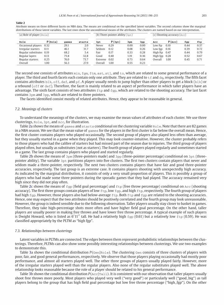
Table 2

Attribute means on three different facets on NBA data. The means are conditional on the specified latent variables. The second columns show the marginal

distributions of those latent variables. The last rows show the unconditional means of the attributes. The clusters are named based on our interpretation.

(a) Role of player (Role)

Role P (Role) games starts

Occasional players 0.32 29.1 2.0

Irregular starters 0.11 46.1 31.7

Regular substitutes 0.19 68.2 5.4

Regular layers 0.13 75.8 32.8

Regular starters 0.25 76.0 73.7

Overall 1.00 56.3 27.9

(b) Three-pointer ability (3pt)

3pt P (3pt) 3pm 3pp

Never 0.29 0.00 0.00

Seldom 0.12 0.08 0.26

Fair 0.17 0.33 0.28

Good 0.40 1.19 0.36

Extreme 0.02 0.73 0.64

Overall 1.00 0.55 0.23

(c) Shooting accuracy (Acc)

Acc P (Acc) fgp ftp

Low ftp 0.10 0.44 0.37

Low fgp 0.16 0.39 0.72

High ftp 0.47 0.44 0.79

High fgp 0.28 0.52 0.67

Overall 1.00 0.45 0.71

The second one consists of attributes min, fgm, ftm, ast, stl, and to, which are related to some general performance of a

player. The third and fourth facets each contain only one attribute. They are related to tf and dq, respectively. The fifth facet

contains attributes blk, off, def, and pf. A player usually needs to jump higher than other players to get a block (blk) ora rebound (off or def). Therefore, the facet is mainly related to an aspect of performance in which taller players have an

advantage. The sixth facet consists of two attributes ftp and fgp, which are related to the shooting accuracy. The last facet

contains 3pm and 3pp, which are related to three pointers.

The facets identified consist mostly of related attributes. Hence, they appear to be reasonable in general.

7.2. Meanings of clusters

To understand the meanings of the clusters, we may examine the mean values of attributes of each cluster. We use three

clusterings, Role, 3pt, and Acc, for illustration.Table 2a shows themeans of games and starts conditional on the clustering variable Role. Note that there are 82 games

in a NBA season.We see that themean value of games for the players in the first cluster is far below the overall mean. Hence,

the first cluster contains players who played occasionally. The second group of players also played less often than average,

but they usually started in a game when they played. This may look counter-intuitive. However, the cluster probably refers

to those players who had the calibre of starters but had missed part of the season due to injuries. The third group of players

played often, but usually as substitutes (not as starters). The fourth group of players played regularly and sometimes started

in a game. The last group contains players who played and started regularly.

Table 2b shows the means of 3pm (three-pointers made) and 3pp (three-pointer percentage) conditional on 3pt (three-

pointer ability). The variable 3pt partitions players into five clusters. The first two clusters contain players that never and

seldom made a three-pointer, respectively. The next two clusters contains players that have fair and good three-pointer

accuracies, respectively. The last group is an extreme case. It contains players shooting with unexpectedly high accuracy.

As indicated by the marginal distribution, it consists of only a very small proportion of players. This is possibly a group of

players who had made some three pointers during the sporadic games that they had played. The accuracy remained very

high since they did not play often.

Table 2c shows the means of fgp (field goal percentage) and ftp (free throw percentage) conditional on Acc (shooting

accuracy). The first three groups contain players of low ftp, low fgp, and high ftp, respectively. The fourth group of players

had high fgp. However, those players also had below-average ftp. Both ftp and fgp are related to the shooting accuracies.

Hence, one may expect that the two attributes should be positively correlated and the fourth groupmay look unreasonable.

However, the group is indeed sensible due to the following observation. Taller players usually stay closer to basket in games.

Therefore, they take high-percentage shots more often and have higher field goal percentage. On the other hand, taller

players are usually poorer in making free throws and have lower free throw percentage. A typical example of such players

is Dwight Howard, who is listed as 6′11′′ tall. He had a relatively high fgp (0.61) but a relatively low ftp (0.59). He was

classified appropriately by the PLTM as “high fgp”.

7.3. Relationships between clusterings

Latent variables in PLTMs are connected. The edges between them represent probabilistic relationships between the clus-

terings. Therefore, PLTMs can also show some possibly interesting relationships between clusterings. We use two examples

to demonstrate this.

Table 3a shows the conditional distribution P(Gen|Role). The clustering Gen consists of three clusters of players with

poor, fair, and good general performances, respectively. We observe that those players playing occasionally had mostly poor

performance, and almost all starters played well. The other three groups of players usually played fairly. However, more

of the irregular starters played well than the regular players. Also none of the regular substitutes played well. The above

relationship looks reasonable because the role of a player should be related to his general performance.

Table 3b shows the conditional distribution P(Acc|Tall). It is consistent with our observation that taller players usually

shoot free throws more poorly. Most players who played very well (“very good”) or particularly well (“good_big”) as tall

players belong to the group that has high field goal percentage but low free throw percentage (“high_fgp”). On the other


Table 3

Conditional distributions of Gen and Acc on NBA data.

(a) P(Gen|Role): relationship between general

ability (Gen) and role (Role)

Role Gen

Poor Fair Good

Occasional players 0.81 0.19 0.00

Irregular starters 0.00 0.69 0.31

Regular substitutes0.22 0.78 0.00

Regular players 0.00 0.81 0.19

Regular starters 0.00 0.06 0.94

(b) P(Acc|Tall): relationship between shooting accuracy

(Acc) and tall-player ability (Tall)

Tall Acc

Low ftp Low fgp High ftp High fgp

Poor 0.28 0.53 0.00 0.18

Fair 0.00 0.02 0.95 0.03

Good 0.00 0.00 1.00 0.00

Good_big 0.11 0.04 0.00 0.86

Very good0.00 0.00 0.14 0.86

Table 4

Partition of attributes on NBA data by the GS method. The last column lists the

number of clusters in the GMM built for each subset of attributes.

Subset of attributes #Clusters

starts, min, fgm, 3pm, ftm, off, def, ast, stl, to, blk, pf 11

games, tf 3

fgp, 3pp, ftp, dq 2

hand, those who do not play well specifically as tall players (“fair” and “good”) usually have average field goal percentage

and higher free throw percentage (“high_ftp”). For those who played poorly as tall players, we cannot tell much about them.

7.4. Comparison with the GS model

The GS models, mentioned in Section 1, contain a collection of GMMs, each built on a subset of attributes. These models

can also be used for facet determination.We now compare the results obtained from the GSmodel and those from the PLTM.

Table 4 shows the partition of attributes given by the GS method. Each row corresponds to a subset of attributes and

identifies a facet. A clustering is given by theGMMbuilt on the subset of attributes. The number of clusters for each clustering

is shown in the last column.

Compared to the results obtained from PLTM analysis, those from the GS method have three weaknesses. First, the

facets found by the GS method appear to be less natural than those by PLTM analysis. In particular, attribute games can be

related to many aspects of the game statistics. However, it is grouped together by the GS method with a less interesting

attribute tf, which indicates the number of technical fouls, in the second subset. In the third subset, attributes fgp, 3pp,ftp are all related to shooting percentages. However, they are also grouped together with an apparently unrelated attribute

dq (disqualifications). The first subset lumps together a large number of attributes. This means it has missed some more

specific and meaningful facets that have been identified by PLTM analysis.

The second weakness is related to the numbers of clusters given by the GS method. One the one hand, there are a large

number of clusters on the first subset. This makes it difficult to comprehend the clustering, especially with many attributes

in this subset. On the other hand, there are only few clusters on the second and third subsets. This means some subtle

clusters found in PLTM analysis were not found by the GS method. The third weakness is inherent in the structure of the

GS models. Since disconnected GMMs are used, the latent variables are assumed to be independent. Consequently, the GS

models cannot show those possibly meaningful relationships between the clusterings as PLTMs do.

7.5. Discussions

The results presented above in general show that PLTM analysis identified reasonable facets and suggest that it gave

meaningful clusterings on those facets. We also see that better results were obtained from PLTM analysis than the GS

method. Therefore, we conclude that PLTMs can perform facet determination effectively on NBA data.

If we think about how basketball games are played, we can expect that the heterogeneity of players can originate from

various aspects, such as positions of the players, their competence on their corresponding positions, or their general compe-

tence. As our results show, PLTM analysis identified these different facets from the NBA data and allowed users to partition

data based on them separately. If traditional clustering methods are used, only one clustering can be obtained, regardless of

whether variable selection is used or not. Therefore, some of the facets cannot be identified by the traditional methods.

The number of attributes in NBA data may be small relatively to those data available nowadays. Nevertheless, we can

still identify multiple facets and obtain multiple meaningful clusterings from the data. We thus can expect real-world data

with higher dimensions are alsomultifaceted. Consequently, it is in general more appropriate to use the facet determination

approach with PLTMs than the variable selection approach for clustering high-dimensional data.


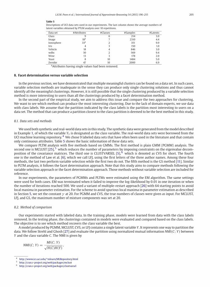
Table 5

Descriptions of UCI data sets used in our experiments. The last column shows the average numbers of

latent variables obtained by PTLM analysis over 10 repetitions.

Data set #Attributes #Classes #Samples #Latents

Glass 9 6 214 3.0

Image 18a 7 2310 4.4

Ionosphere 33a 2 351 9.9

Iris 4 3 150 1.0

Vehicle 18 4 846 3.0

wdbc 30 2 569 9.4

Wine 13 3 178 2.0

Yeast 8 10 1484 5.0

Zernike 47 10 2000 6.9aAttributes having single values had been removed.

8. Facet determination versus variable selection

In the previous section, we have demonstrated thatmultiplemeaningful clusters can be found on a data set. In such cases,

variable selection methods are inadequate in the sense they can produce only single clustering solutions and thus cannot

identify all themeaningful clusterings. However, it is still possible that the single clustering produced by a variable selection

method is more interesting to users than all the clusterings produced by a facet determination method.

In the second part of the empirical study, we aim to address this issue and compare the two approaches for clustering.

We want to see which method can produce the most interesting clustering. Due to the lack of domain experts, we use data

with class labels. We assume that the partition indicated by the class labels is the partition most interesting to users on a

data set. Themethod that can produce a partition closest to the class partition is deemed to be the best method in this study.

8.1. Data sets and methods

Weusedboth synthetic and real-worlddata sets in this study. The synthetic dataweregenerated fromthemodeldescribed

in Example 1, of which the variable Y1 is designated as the class variable. The real-world data sets were borrowed from the

UCI machine learning repository. 4 We chose 9 labeled data sets that have often been used in the literature and that contain

only continuous attributes. Table 5 shows the basic information of these data sets.

We compare PLTM analysis with five methods based on GMMs. The first method is plain GMM (PGMM) analysis. The

second one is MCLUST [25], 5 which reduces the number of parameters by imposing constraints on the eigenvalue decom-

position of the covariance matrices. The third one is CLUSTVARSEL [5], 6 which is denoted as CVS for short. The fourth

one is the method of Law et al. [6], which we call LFJ, using the first letters of the three author names. Among these four

methods, the last two perform variable selection while the first two do not. The fifth method is the GS method [11]. Similar

to PLTM analysis, it follows the facet determination approach. Note that this study aims to compare methods following the

variable selection approach or the facet determination approach. Those methods without variable selection are included for

reference.

In our experiments, the parameters of PGMMs and PLTMs were estimated using the EM algorithm. The same settings

were used for both cases. EM was terminated when it failed to improve the log-likelihood by 0.01 in one iteration or when

the number of iterations reached 500. We used a variant of multiple-restart approach [26] with 64 starting points to avoid

local maxima in parameter estimation. For the scheme to avoid spurious local maxima in parameter estimation as described

in Section 5, we set the constant γ at 20. For PGMM and CVS, the true numbers of classes were given as input. For MCLUST,

LFJ, and GS, the maximum number of mixture components was set at 20.

8.2. Method of comparison

Our experiments started with labeled data. In the training phase, models were learned from data with the class labels

removed. In the testing phase, the clusterings contained in models were evaluated and compared based on the class labels.

The objective is to see which method recovers the class variable the best.

Amodel produced by PGMM,MCLUST, CVS, or LFJ contains a single latent variable Y . It represents oneway to partition the

data. We follow Strehl and Ghosh [27] and evaluate the partition using normalized mutual information NMI(C; Y) between

Y and the class variable C. The NMI is given by

NMI(C; Y) = MI(C; Y)√H(C)H(Y)

,

4 http://www.ics.uci.edu/^mlearn/MLRepository.html5 http://cran.r-project.org/web/packages/mclust6 http://cran.r-project.org/web/packages/clustvarsel

http://www.ics.uci.edu/~mlearn/MLRepository.html

http://cran.r-project.org/web/packages/mclust

http://cran.r-project.org/web/packages/clustvarsel


Table 6

Clustering performances asmeasured byNMI. The averages and standard deviations over 10 repetitions are reported.

Best results are highlighted in bold. The first row categorizes the methods according to their approaches.

Data set Facet determination Variable selection No variable selection

PLTM GS CVS LFJ PGMM MCLUST

Synthetic .85 (.00) .69 (.00) .34 (.00) .56 (.02) .56 (.00) .64 (.00)

Glass .43 (.03) .38 (.00) .29 (.00) .35 (.03) .28 (.03) .33 (.00)

Image .71 (.03) .65 (.00) .41 (.00) .51 (.03) .52 (.04) .66 (.00)

Vehicle .40 (.04) .31 (.00) .23 (.00) .27 (.01) .25 (.08) .36 (.00)

Wine .97 (.00) .83 (.00) .71 (.00) .70 (.19) .50 (.06) .69 (.00)

Zernike .50 (.02) .39 (.00) .33 (.00) .45 (.01) .44 (.03) .41 (.00)

Ionosphere .36 (.01) .26 (.00) .41 (.00) .13 (.07) .57 (.04) .32 (.00)

Iris .76 (.00) .74 (.00) .87 (.00) .68 (.02) .73 (.08) .76 (.00)

wdbc .45 (.03) .36 (.00) .34 (.00) .41 (.02) .44 (.08) .68 (.00)

Yeast .18 (.00) .22 (.00) .04 (.00) .11 (.04) .16 (.01) .11 (.00)

where MI(C; Y) is the mutual information between C and Y and H(V) is the entropy of a variable V [28]. These quantities

can be computed from P(c, y), which in turn is estimated by P(c, y) = 1N

∑Nk=1 Ick(c)P(y|dk), where d1, . . . , dN are the

samples in testing data, Ick(c) is an indicator function having value of 1 when c = ck and 0 otherwise, and ck is the class

label for the k-th sample.

A model resulting from PLTM analysis or the GS method contains a set Y of latent variables. Each of the latent variables

represents a partition of the data. In practice, the user may find several of the partitions interesting and use them all in

his work. In this section, however, we are talking about comparing different clustering algorithms in terms of the ability

to recover the original class partition. So, the user needs to choose one of the partitions as the final result. The question

becomes whether this analysis provides the possibility for the user to recover the original class partition. Consequently, we

assume that the user chooses, among all the partitions produced, the one closest to the class partition and we evaluate the

performance of PLTM analysis and the GS method using this quantity:

maxY∈Y NMI(C; Y).

Note that NMI was used in our experiments due to the absence of a domain expert to evaluate the clustering results. In

practice, class labels are not available when we cluster data. Hence, NMI cannot be used to select the appropriate partitions

in the facet determination approach. A user needs to interpret the clusterings and find those interesting to her. It might also

be possible to use clustering validity indices [29] for selection. Investigation into this possibility is left for future research.

8.3. Results

The results of our experiments are given in Table 6. In terms of NMI, PLTMhad clearly superior performances over the two

variable selection methods, CVS and LFJ. Specifically, it outperformed CVS on all but one data sets and LFJ on all data sets.

PLTM also performed better than GS, the other facet determinationmethod. It outperformed GS on all but one data. Besides,

PLTM has clear advantages over PGMM andMCLUST, the twomethods that do not do variable selection. PLTM outperformed

PGMM on all but one data sets and outperformed MCLUST except for two data sets. On those data sets in our experiments,

PLTM usually outperformed the other methods by large margins.

Note that multiple clusterings are produced by PLTMs and maximum NMI scores are used for comparison. It is therefore

possible that not all of the clusterings produced by PLTM analysis have higher NMI scores than clusterings obtained by other

methods, even if PLTM analysis has a higher maximum NMI score. Moreover, the clusterings produced by other methods

may appear more interesting if the interest of users lies not in the class partitions. Nevertheless, our comparison assumes

that users are only interested in the class partitions. Indeed, this is an assumption taken implicitly when the class partitions

are used for the evaluation of clusterings. Based on this assumption, the experimental results indicate that PLTM analysis

usually provides the best possibility for recovering the partitions of interest.

8.4. Explaining the results

We next examine models produced by the various methods to gain insights about the superior performance of PLTM

analysis. This also allows us to judge the facets identified by PLTM analysis.

8.4.1. Synthetic data

Before examining models obtained from synthetic data, we first take a look at the data set itself. The data were sampled

from themodel shown in Fig. 1b, with information about the two latent variables Y1 and Y2 removed. Nonetheless, the latent

variables represent two natural ways to partition the data. To see how the partitions are related to the attributes, we plot


Y1Y2

Z1Z2

0.0

0.1

0.2

0.3

0.4

0.5

X1 X2 X3 X4 X5 X6 X7 X8 X9Features

NMI

Y1Y2CVS

LFJGS1GS2

0.0

0.1

0.2

0.3

0.4

0.5

X1 X2 X3 X4 X5 X6 X7 X8 X9Features

NMI

Fig. 5. Feature curves of the partitions obtained by various methods and that of the original class partition on synthetic data.

the NMI7 between the latent variables and the attributes in Fig. 5a. We call the curve for a latent variable its feature curve.

We see that Y1 is strongly correlated with X1–X3, but not with the other attributes. Hence it represents a partition based on

those three attributes. Similarly, Y2 represents a partition of the data based on attributes X4–X9. So, we say that the data has

two facets, one represented by X1–X3 and another by X4–X9. The designated class partition Y1 is a partition along the first

facet.

Themodel produced by PLTM analysis has the same structure as the generative model. We name the two latent variables

in the model Z1 and Z2 respectively. Their feature curves are also shown in Fig. 5a. We see that the feature curves of Z1 and

Z2 match those of Y1 and Y2 well. This indicates that PLTM analysis has successfully recovered the two facets of the data. It

has also produced a partition of the data along each of the facets. If the user chooses the partition Z1 along the facet X1–X3 as

the final result, then the original class partition is well recovered. This explains the good performance of PLTM (NMI = 0.85).

The feature curves of the partitions obtained by LFJ and CVS are shown in Fig. 5b.We see that the LFJ partition is not along

any of the two natural facets of the data. Rather it is a partition based on a mixture of those two facets. Consequently, the

performance of LFJ (NMI = 0.56) is not as good as that of PLTM. CVS did identify the facet represented by X4–X9, but it is not

the facet of the designated class partition. In other words, it picked the wrong facet. Consequently, the performance of CVS

(NMI = 0.34) is the worst among all the methods considered. GS succeeded to identify two facets. However, the their feature

curves do not match those of Y1 and Y2 well. This probably explains why its performance (NMI = 0.69) is worse than PLTM.

8.4.2. Image data

In the image data, each instance represents a 3×3 region of an image. It is described by 18 attributes. The feature curve of

the original class partition is given in Fig. 6a.We see that it is a partition based on 10 color-related attributes from intensityto hue and the attribute centroid.row.

The structure of themodel produced by PLTM analysis is shown in Fig. 7. It contains 4 latent variables Y1–Y4. Their feature

curves are shown in Fig. 6a. We see that the feature curve of Y1 matches that of the class partition beautifully. If the user

chooses the partition represented by Y1 as the final result, then the original class partition is well recovered. This likely

explains the good performance of PLTM (NMI = 0.71).

The feature curves of the partitions obtained by LFJ and CVS are shown in Fig. 6b. The LFJ curve matches that of the

class partition quite well, but not as well as the feature curve of Y1, especially on the attributes line.density.5, hue and

centroid.row. This is a possible reason why the performance of LFJ (NMI = 0.51) is not as good as that of PLTM. Similar

things can be said about the partition obtained by CVS. Its feature curve differs from the class feature curve even more than

the LFJ curve on the attribute line.density.5, which is irrelevant to the class partition. Consequently, the performance

of CVS (NMI = 0.41) is even worse than that of LFJ.

GS produced four partitions on image data. Two of them comprise only one component and hence are discarded. The

feature curves of the remaining two partitions are shown in Fig. 6c. We see that one of them corresponds to the facet of the

class partition, but does not match that well. This likely explains why the performance of GS (NMI = 0.65) is better than the

other methods but is not as good as that of PLTM.

Two remarks are in order. First, the 10 color-related attributes semantically form a facet of the data. PLTM analysis has

identified the facet in the pouch below Y1. Moreover, it obtained a partition based on not only the color attributes, but also

the attribute centroid.row, the vertical location of a region in an image. This is interesting. It is because centroid.row is

closely related to the color facet. Intuitively, the vertical location of a region should correlate with the color of the region. For

example, the color of the sky occurs more frequently at the top of an image and that of grass more frequently at the bottom.

7 To computeNMI(X; Y) between a continuous variable X and a latent variable Y , we discretized X into 10 equal-width bins, so that P(X, Y) could be estimated

as a discrete distribution.


classY1Y2Y3Y4

0.0

0.2

0.4

0.6

line.density.5

line.density.2

vedge.mean

vedge.sd

hedge.mean

hedge.sd

intensityrawred

rawblue

rawgreenexredexblue

exgreenvalue

saturationhu

e

centroid.row

centroid.col

Features

NMI

classCVSLFJ

0.0

0.2

0.4

0.6

line.density.5

line.density.2

vedge.mean

vedge.sd

hedge.mean

hedge.sd

intensityrawred

rawblue

rawgreenexredexblue

exgreenvalue

saturationhu

e

centroid.row

centroid.col

Features

NMI

classGS1GS2

0.0

0.2

0.4

0.6

line.density.5

line.density.2

vedge.mean

vedge.sd

hedge.mean

hedge.sd

intensityrawred

rawblue

rawgreenexredexblue

exgreenvalue

saturationhu

e

centroid.row

centroid.col

Features

NMI

Fig. 6. Feature curves of the partitions obtained by various methods and that of the original class partition on image data.

Fig. 7. Structure of the PLTM learned from image data.

Second, the latent variable Y2 is strongly correlated with the two line density attributes. This is another facet of the

data that PLTM analysis has identified. PLTM analysis has also identified the edge-related facet in the pouch node below Y3.

However, it did not obtain a partition along the facet. The partition represented by Y3 depends on not only the edge attributes

but others as well. The two coordinate attributes centroid.row and centroid.col semantically form one facet. The facet

has not been identified probably because the two attributes are not correlated.

8.4.3. Wine data

The PLTM learned fromwine data is shown in Fig. 8. Themodel structure also appears to be interesting. While we are not

experts on wine, it seems natural to have Ash and Alcalinity_of_ash in one pouch as both are related to ash. Similarly,

Flavanoids, Nonflavanoid_phenols, and Total_phenols are related to phenolic compounds. These compounds affect

the color of wine, so it is reasonable to have them in one pouch along with the opacity attribute OD280/OD315. Moreover,

bothMagnesium andMalic_acidplay a role in the production of ATP (adenosine triphosphate), themost essential chemical

in energy production. So, it is not a surprise to find them connected to a second latent variable.

8.4.4. wdbc data

After examining some positive cases for PLTM analysis, we now look at a data set that PLTM did not perform sowell. Here

we consider wdbc data. The data were obtained from 569 digitalized images of cell nuclei aspirated from breast masses.


Fig. 8. Structure of the PLTM learned from wine data.

Fig. 9. Structure of the PLTM learned from wdbc data.

Each image corresponds to a data instance. It is labeled as either benign or malignant. There are 10 computed features of

the cell nuclei in the images. The attributes consist of the mean value (m), standard error (s), and worst value (w) for each

of these features.

Fig. 9 shows the structure of a PLTM learned from this data.We can see that thismodel identifies somemeaningful facets.

The pouch below Y1 identifies a facet related to the size of nuclei. It mainly includes attributes related to area, perimeter,

and radius. The second facet is identified by the pouch below Y2. It is related to concavity and consists primarily of themean

and worst values of the two features related to concavity. The third facet is identified by the pouch below Y3. It includes the

mean and worst values of smoothness and symmetry. The facet appears to show whether the nuclei have regular shapes or

not. The pouch below Y9 identifies a facet primarily related to texture. This facet includes three texture-related attributes but

also the attribute symmetry.s. The remaining attributes aremostly standard errors of some features andmay be considered

as the amount of variation of the features. They are connected to the rest of the model through Y4 and Y8.

classY1Y1(2)

0.0

0.2

0.4

0.6

0.8

radius.w

radius.s

radius.m

perimeter.w

perimeter.s

perimeter.m

compactness.marea.warea.sarea.m

fractal_dim.w

concavity.w

concavity.m

concave_pts.w

concave_pts.m

compactness.w

symmetry.w

symmetry.m

smoothness.w

smoothness.m

concave_pts.s

concavity.s

compactness.s

fractal_dim.s

fractal_dim.m

smoothness.s

texture.w

texture.s

texture.m

symmetry.s

Features

NMI

Fig. 10. Features curves of the partition Y1, obtained by PLTM, and that of the original class partition on wdbc data. Y1(2) is obtained by setting the cardinality of

Y1 to 2.

Table 7

Confusion matrix for PLTM on wdbc data.

Class Y1

s1 s2 s3 s4 s5

Malignant 43 116 6 0 47

Benign 0 9 193 114 41


Although the model appears to have a reasonable structure, it did not achieve a high NMI on this data (NMI = 0.45). To

have better understanding, we compare the feature curve of the class partition with that of the closest partition (Y1) given

by PLTM in Fig. 10. The two feature curves have roughly similar shapes. We also look at the confusionmatrix for Y1 (Table 7).

We see that Y1 gives a reasonable partition. The first four states of Y1 group together the benign cases or malignant cases

almost perfectly, while the remaining state groups together some uncertain cases.

One possible reason for the relatively low NMI is that Y1 has 5 states but the class variable has only 2 states. The higher

number of states of Y1 may lead to a lower NMI due to an increase of the entropy term. Itmay also lead to themismatch of the

feature curves. To verify this explanation, wemanually set the cardinality of Y1 to 2. The feature curve of this adjusted latent

variable (denoted by Y1(2)) is shown in Fig. 10. It nowmatches the feature curve of the class partition well. The adjustment

also improved the NMI to 0.69, andmade it become highest on this data set. This example shows that an incorrect estimated

number of clusters could be a reason why PLTM performed worse than other methods on some data sets.

8.4.5. Discussions

We have also performed PLTM analysis on the other data sets. The last column of Table 5 lists the average numbers of

latent variables obtained over 10 repetitions. We see that multiple latent variables have been identified except on iris data,

which has only four attributes. Many of the latent variables represent partitions of data along natural facets of the data.

In general, PLTM analysis has the ability to identify natural facets of data and cluster data along those facets. In practice,

a user may find several of the clusterings useful. In the setting where clustering algorithms are evaluated using labeled data,

PLTM performs well if the original class partition is also along some of the natural facets, and poorly otherwise.

9. Related work

Some recent work also produces multiple clusterings. One important difference between PLTMs and the recent work

lies in the relationship between clusterings. PLTMs allow the multiple clusterings to be correlated. On the other hand, most

recent work attempts to find multiple clusterings that are dissimilar from each other. Two approaches are commonly used.

The first approach findsmultiple clusterings sequentially. In this approach, an alternative clustering is found based on a given

clustering. The alternative clustering is made dissimilar to the given one with conditional information bottleneck [30], by

“cannot-links” constraints [31], by orthogonal projection [32], orwith an optimization problem constrained by the similarity

between clusterings [33]. The second approach finds multiple clusterings simultaneously. It includes a method based on

k-means [34] and one based on spectral clustering [35]. Both methods find dissimilar clusterings by adding penalty terms

that discourage the similarity between the clusterings to their corresponding objective functions. Besides, there is another

method that finds multiple clusterings simultaneously using the suboptimal solutions of spectral clustering [36].

There are someother lines ofwork that producemultiple clusterings. Caruana et al. [37] generate numerous clusterings by

applying randomweights on the attributes. The clusterings are presented in an organizedway so that a user can pick the one

he deems the best. Biclustering [38] attempts to find groups of objects that exhibit the same pattern (e.g., synchronous rise

and fall) over a subset set of attributes. Unlike our work, the above related work is distance-based rather than model-based.

Our work is also related to projected clustering and subspace clustering [39]. Projected clustering can be considered as

performing local variable selection, where each cluster may have a different subset of attributes. It produces only a single

clustering as variable selection methods do. Subspace clustering considers dense regions as clusters and tries to identify all

clusters in all subspaces. However, it does not partition data along those identified subspaces. In other words, some data

points may not be assigned to any cluster in an identified subspace. This is different from the facet determination approach,

in which data are partitioned along every identified facet.

In terms of model definition, the AutoClass models [40] and the MULTIMIX models [41] are some mixture models that

are related to our work. The manifest variables in those models have multivariate Gaussian distributions and are similar to

the pouch nodes in PLTMs. However, those models do not allow multiple latent variables.

10. Concluding remarks

In this paper, we have proposed PLTMs as a generalization of GMMs and empirically compared PLTManalysiswith several

GMM-based methods. Real-world high-dimensional data are usually multifaceted and interesting clusterings in such data

often are relevant only to subsets of attributes. Oneway to identify such clusterings is to perform variable selection. Another

way is to perform facet determination by PLTM analysis. Our work has shown that PLTM analysis is oftenmore effective than

the first approach.

One drawback of PLTM analysis is that the training is slow. For example, one run of PLTM analysis took around 5 h on data

sets of moderate size (e.g., image, ionosphere, and wdbc data) and around 2.5 days on the largest data set (zernike data) in

our experiments. This prohibits the use of PLTM analysis on data with very high dimensions. For example, PLTM analysis is

currently infeasible for data with hundreds or thousands of attributes, such as those for text mining and gene expression

analysis. On the other hand, even though NBA data has only 18 attributes, our experiment demonstrated that PLTM analysis

on that data could still identify multiple meaningful facets. This suggests that PLTM analysis can be useful for data sets that


have tens of attributes. One possibly fruitful application of PLTMs is for analyzing survey data. Those data usually have only

tens of attributes and are likely to be multifaceted.

A future direction of this work is to speed up the learning of PLTMs, so that PLTM analysis can be applied in more areas.

This can possibly be done by parallelization. Recently, some structural learning methods for LTMs have been proposed to

follow a variable clustering approach [13,42,43] or a constraint-based approach [44,45]. The learning of PLTMs can also

possibly be sped up by following those approaches.

We havemade available online the data sets and the Java implementation of the algorithm used in the experiments. They

can be found on http://www.cse.ust.hk/faculty/lzhang/ltm/index.htm.

Acknowledgements

Research on this work was supported by National Basic Research Program of China (aka the 973 Program) under Project

No. 2011CB505101 and HKUST Fok Ying Tung Graduate School.

Appendix A. Inference algorithm

Consider a PLTMM withmanifest variables X and latent variables Y . Recall that inference onM refers to the computation

of the posterior probability P(q|e) of some variables of interest, Q ⊆ X ∪ Y , after observing values e of evidence variables

E ⊆ X . To perform inference,M has to be converted into a clique tree T. A propagation scheme for message passing can then

be carried out on T.Construction of clique trees is simple due to the tree structure of PLTMs. To construct T, a clique C is added to T for each

edge inM, such that C = V ∪ {�(V)} contains the variable(s) V of the child node and variable�(V) of its parent node. Two

cliques are then connected in T if they share any common variable. The resulting clique tree contains two types of cliques.

The first type are discrete cliques. Each one contains two discrete variables. The second type are mixed cliques. Each one

contains the continuous variables of a pouch node and the discrete variable of its parent node. Observe that in a PLTM all the

internal nodes are discrete and only leaf nodes are continuous. Consequently, the clique tree can be considered as a clique

tree consisted of all discrete cliques, with some mixed cliques attaching to it on the boundary.

Algorithm 1 Inference algorithm

1: procedure Propagate(M, T, E, e)2: Initializeψ(C) for every clique C

3: Incorporate evidence to the potentials

4: Choose an arbitrary clique in T as CP5: for all C ∈ Ne(CP) do6: CollectMessage(CP , C)

7: end for

8: for all C ∈ Ne(CP) do9: DistributeMessage(CP , C)

10: end for

11: Normalizeψ(C) for every clique C

12: end procedure

13: procedure CollectMessage(C, C′)14: for all C′′ ∈ Ne(C′)\{C} do15: CollectMessage(C′, C′′)16: end for

17: SendMessage(C′, C)18: end procedure

19: procedure DistributeMessage(C, C′)20: SendMessage(C, C′)21: for all C′′ ∈ Ne(C′)\{C} do22: DistributeMessage(C′, C′′)23: end for

24: end procedure

25: procedure SendMessage(C, C′)26: φ← RetrieveFactor(C ∩ C′)27: φ′ ← ∑

C\C′ ψ(C)28: SaveFactor(C ∩ C′, φ′)29: ψ(C′)← ψ(C′)× φ′/φ30: end procedure

31: procedure RetrieveFactor(S)

32: If SaveFactor(S, φ) has been called, return φ; otherwise,

return 1.

33: end procedure

// Ne(C) denotes the neighbors of C

After a clique tree is constructed, propagation can be carried out on it. Algorithm 1 outlines a clique tree propagation,

based on the Hugin architecture [46,47], for PLTMs. It consists of four main steps: initialization of cliques, incorporation of

evidence, message passing, and normalization. The propagation on the discrete part of the clique tree is done as usual. Here

we focus on the part related to the mixed cliques.

Step 1: Initialization of cliques (line 2). Consider a mixed clique Cm containing continuous variables W and discrete

variableY = �(W). Thepotentialψ(w, y)ofCm (also denoted asψ(Cm) in the algorithm) is initialized by the corresponding

conditional distribution,

ψ(w, y) = P(w|y) = N(w|μy,�y).

http://www.cse.ust.hk/faculty/lzhang/ltm/index.htm


Step 2: Incorporation of evidence (line 3). The variables in a pouch node W can be divided into two groups, depending

on whether the values of the variables have been observed. Let E′ = W ∩ E denote those variables of which values have

been observed, and let U = W\E denote those of which values have not been observed. Furthermore, let [μ]S denote the

part of mean vector μ containing elements corresponding to variables S, and let [�]ST denote the part of the covariance

matrix � that has rows and columns corresponding to variables S and T , respectively. To incorporate the evidence e′ for E′,the potential of Cm changes fromψ(w, y) to

ψ ′(w, y) = P(e′|y)× P(w|y, e′) = N(e′

∣∣[μy]E′ , [�y]E′E′)×N

(w|μ′y,�′y

),

where μ′y and �′y can be divided into two parts. The part related to the evidence variables E′ is given by:

[μ′y

]E′ = e′,

[�′y

]UE′ = 0,

[�′y

]E′E′ = 0, and

[�′y

]E′U = 0.

The other part is given by:

[μ′y

]U= [μy]U + [�y]UE′

[�−1y

]E′E′

(e′ − [μy]E′

),

[�′y

]UU= [�y]UU − [�y]UE′

[�−1y

]E′E′ [�y]E′U .

Step 3: Message passing (lines 5–10). In this step, Cm involves two operations, marginalization and combination. Mar-

ginalization of ψ ′(w, y) over W is required for sending out a message from Cm (line 27). It results in a potential ψ ′(y),involving only the discrete variable y, as given by:

ψ ′(y) = P(e′|y) = N(e′

∣∣[μy]E′ , [�y]E′E′).

Combination is required for sending a message to Cm (line 29). The combination of the potential ψ ′(w, y) with a discrete

potentialφ(y) is givenbyψ ′′(w, y) = ψ ′(w, y)×φ(y).When themessagepassing completes (line10),ψ ′′(w, y) representsthe distribution

ψ ′′(w, y) = P(y, e)× P(w|y, e′) = P(y, e)×N(w|μ′y,�′y

).

Step 4: Normalization (line 11). In this step, a potential changes fromψ ′′(w, y) to

ψ ′′′(w, y) = P(y|e)× P(w|y, e′) = P(y|e)×N(w|μ′y,�′y

).

For implementation, the potential of a mixed clique is usually represented by two types of data structures: one for the

discrete distribution and one for the conditional Gaussian distribution. More details for the general clique tree propagation

can be found in [46,21,48].

Appendix B. Search algorithm

Some issues for the search algorithm of latent tree models are studied in [49,14]. These issues also affect PLTMs. In this

section, we discuss how these issues are addressed for PTLMs. We summarize the entire search algorithm for PLTMs at the

end of this section.

B.1. Three search phases

In every search step, a search operator generates all possible candidate models for consideration. Let l and b be the

numbers of latent nodes and pouch nodes, respectively, and n = l + b be total number of nodes. Let p, q, and r be the

maximum number of variables in a pouch node, the maximum number of sibling pouch nodes, and the maximum number

of neighbors of a latent node, respectively. The numbers of possible candidate models that NI, ND, SI, SD, NR, PO, and UP

can generate are O(lr(r − 1)/2), O(lr), O(l), O(l), O(nl), O(lq(q − 1)/2), and O(bp), respectively. If we consider all seven

operators in each search step, many candidate models are generated but only one of them is chosen for the next step. Those

suboptimal models are discarded and are not used for the next step. Therefore, in some sense, much time are wasted for

considering the suboptimal models.

A more efficient way is to consider fewer candidate models in each search step. This can be achieved by considering only

a subset of search operators at a time. The search operators can be naturally partitioned into three categories. SI, NI, and PO

belong to the expansion category, since all of them can create candidate models that are more complex than the current


one. SD, ND, and UP, which simplify a model, belong to the simplification category. NR does not change the complexity

considerably. It belongs to the adjustment category. We therefore perform search in three phases, each of which considers

only operators in one category. The best model found in each phase is used to seed the next phase, and the search repeats

these three phases until all three phases cannot find a better model. This search is called EAST, since it does Expansion,

Adjustment, and Simplification until Termination.

B.2. Efficient model evaluation

Supposem is the currentmodel after a number of search steps. A candidatemodelm′ can be obtained fromm by applying

a search operator. Very often, the search operator modifies only a small part of m, so that m and m′ share a large number

of parameters. For example, consider the model m2, that is obtained from model m1 using the PO operator, as shown in

Fig. 3. m1 and m2 shares many parameters such as P(x1, x2|y2), P(y2|y1), P(y3|y1), P(x6|y3), etc. On the other hand, some

parameters are not shared bym andm′. In this example, parameters P(x4|y3) and P(x5|y3) are specific tom1,while parameter

P(x4, x5|y3) is specific tom2.Wecandivide theparametersofm′ into twogroupsandwrite theparametersθ ′ ofm′ as (θ ′1, θ ′2).θ ′1 consists of parameters shared withm, while θ ′2 consists of parameters specific tom′. Similarly, we write the parameters

of m as θ = (θ1, θ2).Suppose we have computed the MLE θ∗ = (θ∗1, θ∗2) of the parameters of m. θ∗1 can be used as estimates for the shared

parameters of m′. Consequently, we can obtain a likelihood function P(D|m′, θ∗1, θ ′2) that depends on only the unshared

parameters θ ′2. This function is referred to as restricted likelihood function ofm′. As previously described, we use the BIC score

to evaluate a candidate model. This requires the maximum log-likelihood (ML) of m′. Instead of computing the ML over all

parameters ofm′, wemay approximate it bymaximizing the restricted log-likelihood over only the subset of parameters θ ′2.This results in an approximate score given by

BICRL(m′|D) = max

θ ′2log P(D|m′, θ∗1, θ ′2)−

d(m′)2

log N.

The advantage of using BICRL is that it allows a more efficient implementation of EM. This is due to two reasons. First, it

involves a maximization of fewer parameters in the M-step. This also means fewer computations in the E-step, since only

distributions relevant to θ ′2 need to be computed. Second, the E-step can exploit the fixed parameters θ∗1 to allow sharing of

computation among all iterations of EM. Specifically, the E-step requires inference on a PLTM, which in turn requires passing

messages in the clique tree. As the parameters θ∗1 do not change in these iterations, the messages that depend on only these

parameters remain the same in all iterations. Therefore, some messages can be cached for each data case and can be shared

for the inference used in subsequent E-steps.

In our implementation, both BIC and BICRL are used to evaluate models, but at different situations. The approximation

BICRL is used for quickly evaluating candidate models generated by the same search operator, while the real BIC is used for

accurately evaluating the candidate model with the highest BICRL for each of the search operators. This improves the speed

for the evaluation of models within search operators, but maintains the accuracy for the evaluation of models across search

operators.

B.3. Operation granularity

Operation granularity refers to the phenomenon where some search operators might increase the complexity of the

current model much more than other search operators. If we use BIC to evaluate candidate models given by the search

operators, thosehavingamuch larger increase incomplexityareusuallypreferred. Thismight lead to localmaxima.Therefore,

we adopt a simple and effective strategy called the cost-effectiveness principle for evaluating the candidate models. Let m

be the current model and m′ be a candidate model. Define the improvement ratio of m′ over m given data D to be

IR(m′,m|D) = BIC(m′|D)− BIC(m|D)d(m′)− d(m)

.

It is the increase in model score per unit increase in model complexity. The cost-effectiveness principle stipulates that one

chooses, among a list of candidate models, the one with the highest improvement ratio.

The principle is applied only on candidate models generated by the SI, NI, and PO operators. In other words, it is used

only during the expansion phase. The principle is not applied for other operators since they do not or do not necessarily

increase model complexity.

B.4. PLTM-EAST

The entire search algorithm for PLTMs is named PLTM-EAST. It is outlined in Algorithm 2. The search process starts

with the initial model m(0) described in Section 6. The procedure PLTM-EAST uses m(0) as the first current model. It then

repeatedly tries to improve the current model in the three different phases.


Algorithm 2 Search algorithm

1: procedure PLTM-EAST(m,D)

2: repeat

3: m′ ← m

4: m← Expand(m)

5: m← Adjust(m)

6: m← Simplify(m)

7: until BIC(m|D) ≤ BIC(m′|D)8: return m′9: end procedure

10: procedure Expand(m,D)

11: loop

12: m′ ← m

13: M← SI(m′) ∪ NI(m′) ∪ PO(m′)14: m← PickModel-IR(M,D)

15: if BIC(m|D) ≤ BIC(m′|D) then16: return m′17: end if

18: if m ∈ NI(m′) ∪ PO(m′) then19: m← Enhance(m,D)

20: end if

21: end loop

22: end procedure

23: procedure Adjust(m,D)

24: return RepPickModel(m,NR,D)

25: end procedure

26: procedure Simplify(m,D)

27: m← RepPickModel(m,UP,D)

28: m← RepPickModel(m,ND,D)

29: m← RepPickModel(m, SD,D)

30: end procedure

31: procedure RepPickModel(m, Op,D)

32: repeat

33: m′ ← m

34: m← PickModel(Op(m′),D)

35: until BIC(m|D) ≤ BIC(m′|D)36: return m′37: end procedure

In procedure Expand, the improvement ratio IR is used to pick the best models among the candidate models generated

by SI, NI, and PO. It stops when the best candidate model fails to improve over the previous model. On the other hand, if

the best candidate model is better, and if it comes from NI or PO, procedure Enhance is called. This procedure iteratively

improves the model by using a restricted version of search operator. If the given model is generated by NI, restricted version

of NR is used. If it is generated by PO, restricted version of PO is used.

In procedure Adjust, it calls the procedure RepPickModel to improves the model using the NR operator repeatedly. In

procedure Simplify, it first tries to improve the model using UP. It then uses ND, and uses SD lastly.

References

[1] L.K.M. Poon, N.L. Zhang, T. Chen, Y. Wang, Variable selection in model-based clustering: to do or to facilitate, in: Proceedings of the 27th InternationalConference on Machine Learning, 2010, pp. 887–894.

[2] J.G. Dy, C.E. Brodley, Feature selection for unsupervised learning, J. Mach. Learn. Res. 5 (2004) 845–889.

[3] D. Steinley, M.J. Brusco, Selection of variables in cluster analysis: an empirical comparison of eight procedures, Psychometrika 73 (1) (2008) 125–144.[4] H. Zeng, Y.-M. Cheung, A new feature selection method for gaussian mixture clustering, Pattern Recognit. 42 (2009) 243–250.

[5] A.E. Raftery, N. Dean, Variable selection for model-based clustering, J. Am. Statist. Assoc. 101 (473) (2006) 168–178.[6] M.H.C. Law, M.A.T. Figueiredo, A.K. Jain, Simultaneous feature selection and clustering using mixture models, IEEE Trans. Pattern Anal. Mach. Intell. 26 (9)

(2004) 1154–1166.[7] Y. Li, M. Dong, J. Hua, Simultaneous localized feature selection and model detection for Gaussian mixtures, IEEE Trans. Pattern Anal. Mach. Intell. 31 (5)

(2009) 953–960.

[8] J.S. Liu, J.L. Zhang, M.J. Palumbo, C.E. Lawrence, Bayesian clustering with variable and transformation selections (with discussion), Bayesian Statist. 7 (2003)249–275.

[9] P.D. Hoff, Model-based subspace clustering, Bayesian Anal. 1 (2) (2006) 321–344.[10] W. Pan, X. Shen, Penalized model-based clustering with application to variable selection, J. Mach. Learn. Res. 8 (2007) 1145–1164.

[11] G. Galimberti, G. Soffritti, Model-based methods to identify multiple cluster structures in a data set, Comput. Statist. Data Anal. 52 (2007) 520–536.[12] N.L. Zhang, Hierarchical latent class models for cluster analysis, J. Mach. Learn. Res. 5 (2004) 697–723.

[13] Y. Wang, N.L. Zhang, T. Chen, Latent tree models and approximate inference in Bayesian networks, J. Artificial Intelligence Res. 32 (2008) 879–900.[14] T. Chen, N.L. Zhang, T. Liu, K.M. Poon, Y. Wang, Model-based multidimensional clustering of categorical data, Artificial Intelligence 176 (2012) 2246–2269.

[15] G.J. McLachlan, D. Peel, Finite Mixture Models, Wiley, New York, 2000.

[16] C. Fraley, A.E. Raftery, Model-based clustering, discriminant analysis, and density estimation, J. Am. Statist. Assoc. 97 (458) (2002) 611–631.[17] A.P. Dempster, N.M. Laird, D.B. Rubin, Maximum likelihood from incomplete data via the EM algorithm, J. R. Stat. Soc. Ser. B Stat. Methodol. 39 (1) (1977)

1–38.[18] J.R.S. Fonseca, M.G.M.S. Cardoso, Mixture-model cluster analysis using information theoretical criteria, Intell. Data Anal. 11 (2007) 155–173.

[19] J. Pearl, Probabilistic Reasoning in Intelligent Systems: Networks of Plausible Inference, Morgan Kaufmann Publishers, San Mateo, California, 1988.[20] D. Geiger, D. Heckerman, Learning Gaussian Networks, Tech. Rep. MSR-TR-94-10, Microsoft Research, 1994.

[21] S.L. Lauritzen, F. Jensen, Stable local computation with conditional Gaussian distributions, Statist. Comput. 11 (2001) 191–203.

[22] S. Ingrassia, A likelihood-based constrained algorithm for multivariate normal mixture models, Statist. Methods Appl. 13 (2) (2004) 151–166.[23] G. Schwarz, Estimating the dimension of a model, Ann. Statist. 6 (2) (1978) 461–464.

[24] N.L. Zhang, T. Kocka, Efficient learning of hierarchical latent class models, in: Proceedings of the 16th IEEE International Conference on Tools with ArtificialIntelligence, 2004, pp. 585–593.

[25] C. Fraley, A.E. Raftery, MCLUST Version 3 for R: Normal Mixture Modeling and Model-Based Clustering, Tech. Rep. 504, Department of Statistics, Universityof Washington, 2006 (revised 2009).

[26] D.M. Chickering, D. Heckerman, Efficient approximations for the marginal likelihood of Bayesian networks with hidden variables, Mach. Learn. 29 (1997)

181–212.


[27] A. Strehl, J. Ghosh, Cluster ensembles – a knowledge reuse framework for combining multiple partitions, J. Mach. Learn. Res. 3 (2002) 583–617.[28] T.M. Cover, J.A. Thomas, Elements of Information Theory, second ed., Wiley, 2006.

[29] M. Halkidi, Y. Batistakis, M. Vazirgiannis, On clustering validation techniques, J. Intell. Inf. Syst. 17 (2/3) (2001) 107–145.[30] D. Gondek, T. Hofmann, Non-redundant data clustering, in: Proceedings of the Fourth IEEE International Conference on Data Mining, 2004, pp. 75–82.

[31] E. Bae, J. Bailey, COALA: a novel approach for the extraction of an alternative clustering of high quality and high dissimilarity, in: Proceedings of the Sixth

IEEE International Conference on Data Mining, 2006, pp. 53–62.[32] Y. Cui, X.Z. Fern, J.G. Dy, Non-reduntant multi-view clustering via orthogonalization, in: Proceedings of the Seventh IEEE International Conference on Data

Mining, 2007, pp. 133–142.[33] Z. Qi, I. Davidson, A principled and flexible framework for finding alternative clusterings, in: Proceedings of the 15th ACM SIGKDD International Conference

on Knowledge Discovery and Data Mining, 2009, pp. 717–726.[34] P. Jain, R. Meka, I.S. Dhillon, Simultaneous unsupervised learning of disparate clusterings, in: Proceedings of the Seventh SIAM International Conference on

Data Mining, 2008, pp. 858–869.

[35] D. Niu, J.G. Dy, M.I. Jordan, Multiple non-redundant spectral clustering views, in: Proceedings of the 27th International Conference on Machine Learning,2010, pp. 831–838.

[36] S. Dasgupta, V. Ng, Mining clustering dimensions, in: Proceedings of the 27th International Conference on Machine Learning, 2010, pp. 263–270.[37] R. Caruana, M. Elhawary, N. Nguyen, C. Smith, Meta clustering, in: Proceedings of the Sixth International Conference on Data Mining, 2006, pp. 107–118.

[38] S.C. Madeira, A.L. Oliveria, Biclustering algorithms for biological data analysis: a survey, IEEE Trans. Comput. Biol. Bioinform. 1 (1) (2004) 24–45.[39] H.-P. Kriegel, P. Kröger, A. Zimek, Clustering high dimensional data: a survey on subspace clustering, pattern-based clustering, and correlation clustering,

ACM Trans. Knowledge Discov. Data 3 (1) (2009) 1–58.

[40] P. Cheeseman, J. Stutz, Bayesian classification (autoclass): theory and results, in: Advances in Knowledge Discovery and Data Mining, AAAI Press, 1996, pp.153–180.

[41] L. Hunt, M. Jorgensen, Mixture model clustering using the MULTIMIX program, Aust. N. Z. J. Stat. 41 (2) (1999) 154–171.[42] Y.Wang, Latent TreeModels forMultivariate Density Estimation: Algorithms and Applications, Ph.D. Thesis, Department of Computer Science and Engineer-

ing, The Hong Kong University of Science and Technology, 2009.[43] S. Harmeling, C.K.I. Williams, Greedy learning of binary latent trees, IEEE Trans. Pattern Anal. Mach. Intell. 33 (6) (2011) 1087–1097.

[44] M.J. Choi, V.Y.F. Tan, A. Anandkumar, A.S. Willsky, Learning latent tree graphical models, J. Mach. Learn. Res. 12 (2011) 1771–1812.

[45] A. Anandkumar, K. Chaudhuri, D. Hsu, S.M. Kakade, L. Song, T. Zhang, Spectral methods for learningmultivariate latent tree structure, in: Advances in NeuralInformation Processing Systems 24, Curran Associates, Inc., 2011, pp. 2025–2033.

[46] R.G. Cowell, A.P. Dawid, S.L. Lauritzen, D.J. Spiegelhalter, Probabilistic Networks and Expert Systems, Springer, 1999.[47] A. Darwiche, Modeling and Reasoning with Bayesian Networks, Cambridge University Press, 2009.

[48] R.G. Cowell, Local propagation in conditional Gaussian Bayesian networks, J. Mach. Learn. Res. 6 (2005) 1517–1550.[49] T. Chen, N.L. Zhang, Y. Wang, Efficient model evaluation in the search-based approach to latent structure discovery, in: Proceedings of the Fourth European

Workshop on Probabilistic Graphical Models, 2008, pp. 57–64.

international journal of approximate reasoninglzhang/paper/pspdf/poon-zhang-ijar-2013.pdf ·...

Documents