international journal of engineering science - luke … · 910 l. bornn et al./international...

Damage detection in initially nonlinear systems

Luke Bornn 1, Charles R. Farrar *,2, Gyuhae Park 2

Los Alamos National Laboratory, Los Alamos, NM 87545, United States

a r t i c l e i n f o

Keywords:Statistical structural health monitoringInitially nonlinearSupport vector machineDuffing oscillator

a b s t r a c t

The primary goal of Structural Health Monitoring (SHM) is to detect structural anomaliesbefore they reach a critical level. Because of the potential life-safety and economic benefits,SHM has been widely studied over the past two decades. In recent years there has been aneffort to provide solid mathematical and physical underpinnings for these methods; how-ever, most focus on systems that behave linearly in their undamaged state—a conditionthat often does not hold in complex ‘‘real-world” systems and systems for which monitor-ing begins mid-lifecycle. In this work, we highlight the inadequacy of linear-based meth-odology in handling initially nonlinear systems. We then show how the recentlydeveloped autoregressive support vector machine (AR-SVM) approach to time-series mod-eling can be used for detecting damage in a system that exhibits initially nonlinearresponse. This process is applied to data acquired from a structure with induced nonlinear-ity tested in a laboratory environment.

! 2010 Elsevier Ltd. All rights reserved.

1. Introduction

With the ubiquitous need to maximize a structure’s life while ensuring the health and safety of individuals using thestructure, Structural Health Monitoring (SHM) has become a fervently studied topic over the past 20 years. The goal ofSHM is to identify damage before it reaches a critical state and at the same time not give false indications of damage. As such,this field has moved rapidly from ad hoc and heuristic approaches for damage detection to methodological developmentbased on the concepts of statistical pattern recognition [1] to the point where fundamental axioms for SHM have beenproposed [2]. As an example of a system where SHM is important, consider the August, 2007 collapse of the I-35W Missis-sippi River Bridge. With a robust SHM system in place the structural deficiencies may have been identified and maintenanceactivities could have been prescribed to prevent the multi-million dollar bridge replacement cost as well as the litigationcosts associated with this disaster. At the very least, the bridge might have been decommissioned to prevent the 13 liveslost. This example is just one that highlights the importance of detecting damage at an early stage, prior to irreversible con-sequences. However, for most applications SHM systems, which include sensing hardware coupled with data interrogationsoftware, have yet to be developed that can be relied upon for such early warnings. As such, despite the extensive literaturesummarizing SHM research over the last 20 years [3,4] there is still a need for further development and field verification ofSHM systems that can provide early indications of potentially dangerous changes in a structure. This capability will allow formaintenance to prevent abrupt failures and extend the structure’s life in a cost-effective manner.

To achieve this goal for SHM systems, it is the authors’ opinion that a statistical pattern recognition paradigm must beemployed in the development of an SHM system. This paradigm consists of a four-step process that includes Operational

0020-7225/$ - see front matter ! 2010 Elsevier Ltd. All rights reserved.doi:10.1016/j.ijengsci.2010.05.011

* Corresponding author.E-mail address: [email protected] (C.R. Farrar).

1 CCS-6, Statistical Sciences Group, MS F600.2 The Engineering Institute, MS T006.

International Journal of Engineering Science 48 (2010) 909–920

Contents lists available at ScienceDirect

International Journal of Engineering Science

journal homepage: www.elsevier .com/locate / i jengsci

Evaluation, Data Acquisition, Feature Extraction and Feature Classification. Inherent in the last three steps of this paradigm isthe need for data normalization, cleansing, and compression, which are implemented with either hardware or software. Amore detailed discussion of this statistical pattern recognition paradigm for SHM can be found in [5]. This paper focuseson the feature extraction and classification portions of this paradigm.

Many existing SHM feature extraction methodologies are based on fitting linear models (e.g. a modal model) to measuredsystem response data before and after damage. Changes in the parameters of these models are then used as indicators ofdamage. This physics-based modeling approach has been extended to data-based time-series models where in addition tomodel parameters, residual errors between measured and predicted responses are used as damage-sensitive features. Morerecently, researchers have studied SHM approaches that are based on the principle that an undamaged structure thatbehaves in an initially linear manner will, under the presence of damage, exhibit nonlinear response [6,7]. The formationof cracks that open and close under load is one such example of damage that would induce nonlinearity. Methods areproposed in [6,7] to take advantage of this transition from linear to nonlinear response in the damage-detection process.However, many real-world structures, particularly those with numerous and complex joints and interfaces, will behavenonlinearly even in their undamaged state. In addition, some situations involve the monitoring of systems that are damagedto begin with. The goal is then to ensure the damage does not increase beyond some critical threshold. This situation mayarise, for instance, when the SHM monitoring system is deployed mid-lifecycle. These systems may also demonstrate non-linear response characteristics in their initial ‘‘undamaged” state and hence most existing SHM techniques would beinadequate.

In this paper we begin by focusing on existing SHMmethodology, in particular the inability of existing methods to handleinitially nonlinear systems. To this end, Section 2 discusses several common techniques for SHM, demonstrating their lim-itations when applied to initially nonlinear systems. Section 3 focuses on the recent autoregressive support vector machine[8], which by design is well-suited to modeling nonlinear systems. As discussed in [8], support vector machines have beenreported many times in the recent SHM literature where they are used as a classification algorithm. However, the study sum-marized in [8] is, to the authors’ knowledge, the first time SVMs have been applied to time-series regression modeling in theSHM context. The study reported herein extends this methodology to data from initially nonlinear systems where the abilityto identify damage even between two nonlinear states is demonstrated. The process is demonstrated on a laboratory struc-ture where different nonlinearities can be introduced at various locations. Lastly, Section 4 concludes the work and discussesavenues for further research.

2. Existing SHM feature extraction techniques applied to initially nonlinear systems

With the majority of existing SHM techniques focusing on initially linear systems, we seek to explore how these methodsfare when systems behave nonlinearly in their initial state. These techniques primarily seek to fit a predictive model, eitherphysics- or data-based, to the undamaged system. As the system remains in the linear undamaged state these models shouldcontinue to accurately predict the system’s response. However, at the occurrence of damage, the underlying process gener-ating the data has changed, and hence the model should no longer accurately predict the system’s response. Thus one canmonitor the model’s parameters or its predictive errors as the damage-sensitive feature of interest. An alternate approach isto identify features that directly compare the measured response waveforms or spectra of these waveforms. The extensivenumber of SHM techniques discussed in the literature precludes a comprehensive summary of each method’s ability to han-dle initially nonlinear systems. Instead, we discuss a few methods reported in the literature to highlight the difficulties thatmay be encountered when one deals with an undamaged system that exhibits nonlinear response characteristics. This dis-cussion is prefaced with the acknowledgement that the response characteristics exhibited by a structure will depend on thespecific type of nonlinearity present and various characteristics may be observed with the same structure if different types ofnonlinearities are present.

2.1. Damage-sensitive features derived from model parameters and predictive errors

One data-based technique that has been reported extensively in the SHM literature makes use of traditional autoregres-sive (AR) models to extract damage-sensitive features. These models are based on a linear fit to the raw time-series sensoroutput data (at time t with sensor k) of the form

xkt !Xp

j!1

wkj " x

kt#j $ ekt : %1&

Or stated another way, these models predict the current measured time point based on a linear combination of the pprevious measured time points weighted by the parameters w. Here ekt represents the error between the prediction andthe actual measured value of the time series at time t. Once the model has been fit to data known to be undamaged, it isthen tested on new, potentially damaged data in two manners. First, a similar p-order model can be fit to new data andchanges in the parameters, w, between the two models can be used to form a p-dimensional feature vector that is then usedto indicate damage. Alternatively, the model trained on the undamaged data can be used to predict the new response dataand changes in the properties of the residual error vector can then be used as a damage-sensitive feature. Both theseapproaches are based on the assumption that if the system continues in its undamaged state, the model (either its

910 L. Bornn et al. / International Journal of Engineering Science 48 (2010) 909–920

parameters or the residual errors) should not change significantly. However, changes in the process generating the data(such as damage) will affect either the model parameters or the residual errors associated with a particular model’s predic-tion. By repeating the model fitting process or the time series prediction over time, either the model parameters or the resid-uals can then be monitored for significant changes using a variety of statistical procedures such as control charts [9,10].Statistically significant increases in the variability of these features would then be considered indicative of damage.

As previously stated, each point in the time series is modeled as a linear combination of the previous pmeasured points inthe signal. Thus in order to ensure appropriate fit, and hence the ability of the model to accurately predict other measuredresponses generated by this system, the response signal must be generated by a linear or near linear process, in which casethe AR model gives the best linear approximation to that process. In addition, because of the constrained nature of the ARmodel, the fit can be poor in signals exhibiting non-stationarity (such as those created by transient hammer-impacts) andlengthy (or no) periodic behavior. Thus when the underlying process is nonlinear in its initial state, and the form of the mea-sured response signal is either unknown or complicated, the linear ARmodels are not a suitable choice. This difficulty is illus-trated with the following numerical example. Consider a signal generated from an undamaged system that has a cubicnonlinearity as described by:

m!y$ c _y$ ky$ ay3 ! x%t&; %2&

wherem, c and k are the system’s mass, damping and linear stiffness coefficients, respectively, a is a constant associated withthe cubic stiffness term, and x(t) is a forcing term. The system response is calculated using a 4th order Runge–Kutta numer-ical integration scheme [11] with a time step of 0.2 and a maximum time value of t = 4000. In addition, the parametersm, c, kand a are set to 1, 0.1, 1, and 1, respectively. The system is subjected to a time-varying harmonic forcing function of the form

x%t& ! %10$ t=100& cos%2t&: %3&

If the system were linear, an increasing amplitude associated with the forcing term would result in a corresponding in-crease in the response signal, and hence the AR model fit to the normalized response data would fit equally well regardless ofinput force. However, in a nonlinear system changes in input result in nonlinear changes to the output, and hence the form ofthe response signal will change. We plot the response for various time intervals in Fig. 1. The first and last intervals shownwill be used in the subsequent analysis.

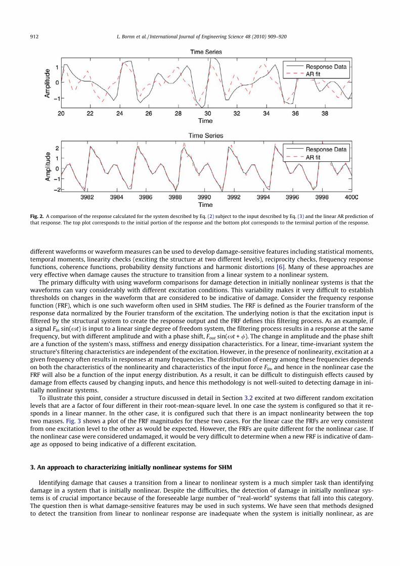
Because the AR model uses a single set of coefficients to model the entire time-series, we expect that it will not ade-quately capture the system dynamics at all excitation levels when it is fit to data with the nonlinearity present. This pointis illustrated in Fig. 2, where the simulated system response to the input described by Eq. (3) and the ARmodel fit to that datafor two different time windows (and hence two different forcing levels) are shown.

This example illustrates the well-known property that the linear AR model does not generalize to predict responsesresulting from other input cases when the underlying system is nonlinear. In such cases both of the standard damage-sen-sitive features associated with these regression models, the model parameters and residual errors, would most likely givefalse indications of damage. The points being illustrated by this example extends to all the physics-based modeling ap-proaches to damage detection discussed in [3,4] (e.g. modal parameter changes, finite element model updating procedures)that are based on the assumption that the underlying system will exhibit linear response and time-invariant system prop-erties when in its undamaged condition.

2.2. Damage-sensitive features based on waveform comparisons

Alternative damage-detection methods are based on examining the measured response waveforms or spectra of thesewaveforms from structures in the undamaged condition. Similar waveforms or spectra are obtained from the potentiallydamaged system and compared to the baseline data in an effort to detect changes in the system producing these data. Many

Fig. 1. The response calculated for the system described by Eq. (2) subject to the input described by Eq. (3) for several time intervals. The input amplituderanges from approximately 10 in the leftmost plot to almost 50 in the rightmost plot.

L. Bornn et al. / International Journal of Engineering Science 48 (2010) 909–920 911

different waveforms or waveformmeasures can be used to develop damage-sensitive features including statistical moments,temporal moments, linearity checks (exciting the structure at two different levels), reciprocity checks, frequency responsefunctions, coherence functions, probability density functions and harmonic distortions [6]. Many of these approaches arevery effective when damage causes the structure to transition from a linear system to a nonlinear system.

The primary difficulty with using waveform comparisons for damage detection in initially nonlinear systems is that thewaveforms can vary considerably with different excitation conditions. This variability makes it very difficult to establishthresholds on changes in the waveform that are considered to be indicative of damage. Consider the frequency responsefunction (FRF), which is one such waveform often used in SHM studies. The FRF is defined as the Fourier transform of theresponse data normalized by the Fourier transform of the excitation. The underlying notion is that the excitation input isfiltered by the structural system to create the response output and the FRF defines this filtering process. As an example, ifa signal Fin sin(xt) is input to a linear single degree of freedom system, the filtering process results in a response at the samefrequency, but with different amplitude and with a phase shift, Fout sin(xt + /). The change in amplitude and the phase shiftare a function of the system’s mass, stiffness and energy dissipation characteristics. For a linear, time-invariant system thestructure’s filtering characteristics are independent of the excitation. However, in the presence of nonlinearity, excitation at agiven frequency often results in responses at many frequencies. The distribution of energy among these frequencies dependson both the characteristics of the nonlinearity and characteristics of the input force Fin, and hence in the nonlinear case theFRF will also be a function of the input energy distribution. As a result, it can be difficult to distinguish effects caused bydamage from effects caused by changing inputs, and hence this methodology is not well-suited to detecting damage in ini-tially nonlinear systems.

To illustrate this point, consider a structure discussed in detail in Section 3.2 excited at two different random excitationlevels that are a factor of four different in their root-mean-square level. In one case the system is configured so that it re-sponds in a linear manner. In the other case, it is configured such that there is an impact nonlinearity between the toptwo masses. Fig. 3 shows a plot of the FRF magnitudes for these two cases. For the linear case the FRFs are very consistentfrom one excitation level to the other as would be expected. However, the FRFs are quite different for the nonlinear case. Ifthe nonlinear case were considered undamaged, it would be very difficult to determine when a new FRF is indicative of dam-age as opposed to being indicative of a different excitation.

3. An approach to characterizing initially nonlinear systems for SHM

Identifying damage that causes a transition from a linear to nonlinear system is a much simpler task than identifyingdamage in a system that is initially nonlinear. Despite the difficulties, the detection of damage in initially nonlinear sys-tems is of crucial importance because of the foreseeable large number of ‘‘real-world” systems that fall into this category.The question then is what damage-sensitive features may be used in such systems. We have seen that methods designedto detect the transition from linear to nonlinear response are inadequate when the system is initially nonlinear, as are

Fig. 2. A comparison of the response calculated for the system described by Eq. (2) subject to the input described by Eq. (3) and the linear AR prediction ofthat response. The top plot corresponds to the initial portion of the response and the bottom plot corresponds to the terminal portion of the response.


methods based on waveform comparison whose detection features are not well-defined in the presence of nonlinearity. Toaddress these shortcomings, we again focus on the system’s time-series data to detect changes in the measured responsethat are associated with damage. Specifically, we focus on a class of models capable of characterizing highly complex andnonlinear responses. These models, known as autoregressive support vector machines (hereafter AR-SVM), are capable ofmodeling any nonlinear relationship given appropriate training data. SVMs have been used for SHM before [12–16], how-ever these approaches predominantly focus on one and two class SVMs, which are used for outlier detection and groupclassification, respectively. In contrast, this study focuses on using SVMs for regression modeling where the damage-sen-sitive feature will be the residual error between the AR-SVM prediction of the sensor reading and the actual measuredtime series. Although AR-SVM’s robust and precise ability to detect damage has been demonstrated in the linear setting[8], the work described herein constitutes the first effort to use AR-SVMs for damage detection in initially nonlinearsystems.

3.1. Autoregressive support vector machines

Following the development first presented in [8,17,18], for the kth sensor and time point t the AR-SVM model has theform

xkt !

Xt0

j!p$1

bjK%xkj#p:j#1; x

kt#p:t#1& $ ekt ; %4&

where we have denoted the vector fxkj ; . . . ; xkt#1g as xkj:t#1. Here t0 is the length of the training set on which the model is built,

and K is a kernel function, which may by thought of as a measure of distance between two vectors. Although at first glancethis model form looks surprisingly like the traditional linear AR model (Eq. (1)), both the development and form are signif-icantly different.

First, assume we have data from a set of measurements without damage, but with nonlinearity present, for timet = 1, . . . , t0. Next the model order p must be defined. There are many methods for selecting p, such as partial autocorrelationor the Akaike Information Criterion (AIC), which are discussed in more detail in [10]. As with linear AR modeling, we createthe training set on which to build our AR-SVMmodel by using each observation as the dependent variable and the previous pobservations as independent variables. Our training samples are thus f%xk

t#p:t#1; xkt &; t ! p$ 1; . . . ; t0g .

Ideally we would like to find a function f such that f%xkt#p:t#1& ! xkt for t 6 t0. However, if the form of f is restricted to linear

functions, this restricted form makes perfect fit of the data impossible in most scenarios. As a result, the prediction using f isallowed to have an error bounded by c, and then w is found under this constraint. Through the recent advances in penalizedregression methods [19,20] it has been shown that optimal prediction performance is obtained by minimizing w, whichleads us to minimize the Euclidean norm of w subject to the error constraint c, stated as

minimize12kwk2;

subject toxkt # hw;xk

t#p:t#1i 6 c;

hw; xkt#p:t#1i# xkt 6 c;

8<

:

%5&

where h; i denotes the dot product. This development relies on the assumption that a linear model is able to fit the data towithin precision c. However, such a linear model often does not exist, even for moderate settings of c. As such, we introducethe slack variables n$t , n

#t to allow for deviations beyond g. The resulting formulation is

20 40 60 80 100 12010-4

10-3

10-2

10-1

Frequency (Hz)

FRF

(g/N

)Linearity Check, no bumper ch3

2V RMS0.5V RMS

20 40 60 80 100 12010-4

10-3

10-2

10-1

Frequency (Hz)

FRF

(g/N

)

Linearity Check, with bumper ch3

2V RMS0.5V RMS

Fig. 3. Frequency response functions corresponding to different excitation levels in a linear system (left) and a nonlinear system (right).


minimize12kwk2 $ C

Xt0

t!p$1

%n$t $ n#t &;

subject toxkt # hw; xkt#p:t#1i 6 c$ n$t ;

hw; xkt#p:t#1i# xkt 6 c$ n#t ;

( %6&

where the constant C controls the tradeoff between giving small w and penalizing deviations larger than c. By framing theabove in its Lagrange formulation it can be seen that the optimal f has the form

f xkt#p:t#1

! "!

Xt0

j!p$1

bj xkj#p:j#1; xkt#p:t#1

D E: %7&

In this way wmay be viewed as a linear combination of the training points xkj#p:j#1. Note also that in this formation both f and

the corresponding optimization can be described in terms of dot products between the data. Next, the data are transformedfrom the p-dimensional space to a higher dimension space using a functionU: Rp ? F, and the dot products are computed inthe transformed space. Specifically, the mapping allows us to fit linear functions in F which, when converted back to Rp, arenonlinear.

To make use of this transformed space, we replace the dot product term in Eq. (7) with

U xkt0#p:t0#1

! ";U xkt#p:t#1

! "D E: %8&

If F is of high dimension, then the above dot product will be extremely expensive to compute. In some cases, however, thereis a corresponding kernel that is simple to compute. One such family of kernels is the Radial Basis Function (RBF) kernels ofthe form

K%x; y& ! exp%#kx# yk2=%2r2&&; %9&

where r2 is the kernel variance. This parameter controls fit, with large values leading to smoother functions and small valuesleading to better fit. Replacing the dot-product in Eq. (8) with the kernel K gives the model defined by Eq. (4).

We now focus on the model’s form to identify why it is well-suited for the purpose of modeling nonlinear systems.First, note that the traditional AR model in Eq. (1) fits each point in the time series as a linear combination of the pre-vious p time points. The AR-SVM model instead looks at the previous p points and compares them to every sequence ofp points in the training set. Intuitively, if the model notices a sequence of points in the training set very similar to thosebeing tested, it bases its prediction quite heavily on that portion of the training set. This feature allows AR-SVM to per-form well when the system exhibits non-stationary response characteristics and when the model order p is too small toobserve the entire system response characteristics.

Also, the kernel function K provides the ability to handle nonlinear relationships in the data. Best thought of as a distancemeasure, kernel functions might take a variety of forms, the most common of which is the radial basis function. While thischoice of kernel has been shown to have many good properties, other choices (including the linear dot product) are possible.Through the right choice of kernel function and kernel parameters (such as r2 in Eq. (9)), AR-SVM is able to model any non-linear relationship in the data. While traditional AR models will find the best linear fit to a nonlinear system, the ability tomodel nonlinear relationships in the data allows AR-SVM to better fit the initially nonlinear data, and hence the predictionsfrom these models will be more sensitive to subsequent changes in the system resulting from damage even when thesechanges also introduce additional nonlinearities into the system.

It should be noted that RBF neural networks have the same form as Eq. (4). However, fitting these networks requires muchmore user input such as selecting which bj are non-zero as well as selecting the corresponding training points. In addition,the fitting of the neural network model is a rather complicated nonlinear optimization process relative to the simplequadratic optimization used in the support vector framework. Although the SVM models are more easily developed, ithas been demonstrated [21] that SVMs still more accurately predict the data than the RBF neural networks despite theirsimplicity.

To demonstrate the ability of AR-SVM to model nonlinear system response, consider the Duffing oscillator previouslydescribed in Section 2.1 that was subject to an amplitude varying harmonic excitation defined by Eq. (3). In Fig. 2 it was seenthat a linear AR model was unable to predict the system response at different excitation levels. However, Fig. 4, which showsthe AR-SVM’s prediction of the same two portions of the time series, reveals that AR-SVM is able to capture the systemresponse at the extreme levels of the loading much more accurately than the linear model.

3.2. Experimental example

Most SHM situations require one to consider environmental and operational variability that typically complicates thedamage-detection process. However, in order to highlight the AR-SVM method’s ability to successfully detect damage ininitially nonlinear systems we focus on a controlled laboratory experiment shown schematically in Fig. 5. The experi-mental structure consists of aluminum plates and columns connected with bolted joints. An electro-dynamic shaker


excites the system through a rigid base constrained to slide horizontally by a system of rails. Each floor contains anaccelerometer and is separated from adjacent floors by four corner columns. To simulate nonlinearity in the initial sys-tem, a column is suspended from the top floor and a bumper is placed on the second floor. With the bumper gap set at0.05 mm, the contact of this suspended column with the bumper results in frequent impacts that produce the nonlinearsystem response that is not considered to be damaged. It is noted that this structure does not represent a scale model ofany particular ‘‘real-world” structure, but rather was constructed to exhibit the nonlinear dynamics characteristics thatwould be observed in real-world structures such as those that might occur if a crack opens and closes under operationalconditions.

0.177

0.177

0.177

Accelerometer 4

0.174

A B

3

2

1

C D

3

2

1

Accelerometer 3

Accelerometer 2

Accelerometer 1

Column

Bumper

Shaker

2nd Floor

1st Floor

3rd Floor

Base

2nd Floor

1st Floor

3rd Floor

Base

Fig. 5. Diagram of experimental setup.

Fig. 4. The AR-SVM prediction of the Duffing oscillator described by Eq. (2) subjected to the input described by Eq. (3).


From this initially nonlinear system we simulate damage by loosening bolts as follows:

Damage 1: loosening bolts connecting column 3BD.Damage 2: loosening bolts connecting column 2AC.Damage 3: loosening bolts connecting column 1AD.

Note that these damage cases have similar characteristics to the nonlinearity associated with the undamaged condition inthat they both result in repeated impacts when the structure is subjected to the base excitation. The damage cases have thesubtle difference in that they also introduce an asymmetry into the structural system stiffness and they correspond to a lossof stiffness from the undamaged condition. The impacting of the bumper associated with the undamaged condition causesan increase in stiffness from the low level response condition when contact is made.

The structure is excited using a band-limited random excitation at 4v RMS in both its undamaged and various damagedconditions. From the resulting accelerometer outputs we seek to identify the presence of damage in each case, as well as anyindicators of the damage location, if possible. For a more detailed description of the test structure and the data that werecollected, visit http://institute.lanl.gov/ei/software-and-data/.

Sampling at 320 Hz, multiple replicates of response data consisting of 2048 data points were obtained from the structurein both its initial nonlinear undamaged condition and in its damaged condition as described above. Now, we use three of theundamaged nonlinear response replicates (total of 6144 time points) to train the AR-SVM model. Specifically, we normalizethese data by subtracting the mean amplitude and then dividing by its standard deviation for each sensor output. Followingthis data normalization step, we fit the data using the value of r2 = 1 in Eq. (9) and p = 30 for Eq. (4). The value of pwas deter-mined from the partial autocorrelation plots shown in Fig. 6. These plots display the similarity between observations in theraw undamaged time series as a function of the lag, or time separation, between them. From these plots the smallest modelorder p should be selected such that the correlation values for lags less than p remain large and for those greater than premain small.

Now that the AR-SVM models have been trained for each sensor on a length of data known to be damage-free (butwith nonlinearities), a test set for each damage case is created consisting of one 2048 time point replicate of the

Fig. 6. Partial autocorrelation plots for the four sensors based on the undamaged nonlinear training data.


damaged data concatenated with a similar length record of undamaged data. These concatenated data of length 4096 areour testing data. The goal of the damage-detection process is to recognize a difference between the undamaged nonlin-ear state (times 0 through 2048) and the damaged state (times 2049 through 4096). The process of analyzing the con-catenated data simulates that which might occur with a continuous monitoring system. First, however, the damageddata are normalized using the mean and standard deviation of the training data. Figs. 7–9 plot the residual errors fromthe model fit to the damaged data for each damage case and sensor.

From these figures it can be seen that AR-SVM is able to differentiate between the undamaged and damaged case. Spe-cifically, the model fits the undamaged portion of the testing set well and fits the damaged portion poorly. Thus the methodis quite sensitive to underlying changes in the process, even when the undamaged system responds in a nonlinear manner.Specifically, the associated standard deviations of the residuals from the model fit to the testing data are listed in Table 1.Also listed are the ratios of variances for the undamaged and damaged residuals for each scenario. These ratios will be usedto conduct statistical tests that check for changes in AR-SVM model fit to the measured response data and that will be usedas the damage indicator.

From these values we see that indeed the residuals for the undamaged portion of the data are much smaller than those inthe damaged portion. To be more precise, we may employ an F-test to determine if the residuals from the damaged case havesignificantly larger variance than those from the undamaged case [22]. The F-test compares the ratio of variances r2

1=r22 from

two normal (or nearly normal) samples, testing the hypothesis that the variances are from the same population (i.e.H0 : r2

1 ! r22). It has been shown, for instance in [8], that the assumption of normal residuals is reasonable for most SHM

scenarios. Rejection of this null hypothesis indicates that the sample variances are from different populations as indicatedby values of the ratio far from 1. Because of our interest in testing if the variance is increasing as a result of damage, aone-sided test is appropriate. To implement the F-test, a significance level must be defined. The significance level is the max-imum probability that we have rejected the null hypothesis when, in fact, it should have been accepted. In terms of damagedetection this translates into the maximum probability of inferring that damage has occurred when the structure is actuallyundamaged (also referred to as a false-positive indication of damage). Although in ‘‘real-world” damage detection studies theestablishment of the significance level will be application dependent and a function of the consequences (e.g. life-safety, eco-nomic) of misclassification, in this study a commonly used significance level of 0.05 was chosen.

Because data are available from multiple sensors and, hence, we can perform several F-tests, we must account formultiple testing. Therefore, to ensure the F-test is conservative, an overall significance of 0.05 will be obtained by testing

Fig. 7. Residuals from AR-SVM. Damage 1 (loose column connection between floor three and two) at point 2049.


each sensor at significance of 0.01. In fact, such a significance level will result in an overall significance of1 # (1 # 0.01)4 = 0.04. With 2048 points in both the damaged and undamaged cases, the F-test indicates significance at a le-vel of 0.01 if the ratio of variances between undamaged and damaged residuals is less than 0.90 (the undamaged divided bythe damaged sample variance). More precisely, a ratio of variances of 0.9 when both samples are of size 2048 corresponds toa p-value for the F-distribution of 0.009. Similarly, because sensor 2 has a ratio of variances less than 0.36 for all damagescenarios, the F-test will on average indicate significance even when we have seen as little as seven damaged time points.This result can be seen from a standard table for an F-distribution, which shows a ratio of variances of 0.36 from 2048and seven samples from the numerator and denominator samples, respectively, corresponds to a p-value of 0.01. Hencethe method is able to detect changes in the system even at a very early stage. We conclude that AR-SVM is fitting the undam-aged data significantly better than the damaged data, and hence the method is able to differentiate between the twoconditions.

Note that the results of the significance test do not necessarily indicate the damage location. However, we can determinewhich sensor (in this case sensor 2) is most sensitive to changes in the system. Sensor 3 is an interesting case, fitting the thirddamage scenario slightly better than the undamaged case. Because of this sensor’s close proximity to the initial nonlinearityand large distance from the damage source, it is likely that the damage had little effect, and the slightly better fit to this case(residual standard deviation of 0.17 versus 0.18) is merely due to rounding error and statistical variation.

4. Conclusions

In this paper we have noted that not all ‘‘real-world” systems of interest to Structural Health Monitoring experts fit theinitially linear profile typically studied in the SHM literature. If there is intent to retrofit SHM systems to old structures aswell as new structures with complex joints and interfaces and to have such systems analyze data from widely varying oper-ational and environmental loading conditions, these systems must be able to handle nonlinearity in the initial system state.The discussion first focused on general classes of currently used SHMmethods and demonstrated that each is not well-suitedto handle systems exhibiting initial nonlinearity. Then the AR-SVM methodology was developed and shown to accuratelymodel nonlinearity associated with the initial undamaged system. This method was then shown to be able to detect changesin the dynamic system response associated with damage that produced another source of nonlinearity with similar charac-teristics as the nonlinearity associated with the undamaged condition. The authors consider this to be a very challenging

Fig. 8. Residuals from AR-SVM. Damage 2 (loose column connection between floor two and one) at point 2049.


damage detection case that is indicative of challenges that real-world applications pose for SHM processes and that high-lights the strengths of the AR-SVM methodology for SHM applications. As with all damage-detection methods, AR-SVM isnot immune to the challenges accompanying systems that behave very similarly in both their undamaged and damagedstate. Specifically, if damage is present in the training set, this damage will not be detected as such in the testing set. In addi-tion, damage that manifests itself in a form similar to the initial nonlinearities will not be detected. However, it begs repeat-ing that all vibration-based SHM methods suffer similar flaws.

As a next step, work must be done to identify damage in nonlinear systems even in the presence of environmental var-iability. Because real-world systems are subject to varying loads and other conditions, SHM methods for these systems mustbe sensitive to damage, yet robust to changes in environment. However, distinguishing between the two can be a difficultproblem. This step requires the application of these processes to data from in situ structures subject to environmentaland operational variability. However, it is often difficult to find such structures that subsequently experience damage ona reasonable time scale as is needed for a proof-of-concept demonstration.

By detailing the need to advance the study of initially nonlinear systems, we hope this work sparks interest and devel-opment in this area. Without the development of tools for handling such systems, practitioners may be forced to use alter-native linear-based methods that may fail. In general, it is the authors’ speculation that such methods will fail through false-negative indications of damage caused by lack of sensitivity to system change that occurs when linear models attempt to

Table 1Standard deviations of AR-SVM model residuals.

Sensor 1 Sensor 2 Sensor 3 Sensor 4

Undamageda 0.42 0.20 0.18 0.18Damage 1b 0.63 (0.44) 0.49 (0.17) 0.27 (0.45) 0.26 (0.48)Damage 2b 0.69 (0.37) 0.51 (0.15) 0.28 (0.41) 0.25 (0.52)Damage 3b 0.66 (0.41) 0.33 (0.36) 0.17 (1.12) 0.24 (0.56)

The ratio of variances for undamaged/damaged is shown in parentheses for each scenario.a Source of initial nonlinearity considered to be part of the undamaged system is located between sensors 3 and 4.b The bold entries are the sensors on the floors between which the column was loosened to simulate damage.

Fig. 9. Residuals from AR-SVM. Damage 3 (loose column connection between floor one and the base) at point 2049.


model nonlinear system response. Thus, the need for methodology related to nonlinear systems is not only to increase thescope of SHM applications, but also to increase the feasibility and workability of SHM systems in any system potentiallyexhibiting nonlinearity. With the addition of this work, the AR-SVMmethod has been shown to be effective in modeling bothlinear and nonlinear systems, and hence is a good starting point for practitioners dealing with initially nonlinear systems.

Acknowledgement

This work was partially funded by a grant from the Office of Naval Research.

References

[1] C.R. Farrar, S.W. Doebling, D.A. Nix, Vibration-based structural damage identification, Philosophical Transactions of the Royal Society: Mathematical,Physical and Engineering Sciences 359 (2001) 131–149.

[2] K. Worden, C.R. Farrar, G. Manson, G. Park, The fundamental axioms of structural health monitoring, Proceedings of the Royal Society A: Mathematical,Physical and Engineering Sciences 463 (2007) 1639–1664.

[3] H. Sohn, C.R. Farrar, F. Hemez, D. Shunk, D. Stinemates, B. Nadler, A Review of Structural Health Monitoring Literature from 1996–2001, Los AlamosNational Laboratory Report LA-13976-MS, 2004.

[4] S.W. Doebling, C.R. Farrar, M.B. Prime, D.W. Shevitz, Damage Identification and Health Monitoring of Structural and Mechanical Systems From Changesin their Vibration Characteristics: A Literature Review, Los Alamos National Laboratory Report LA-13070-MS, 1996.

[5] C.R. Farrar, K. Worden, An introduction to structural health monitoring, Philosophical Transactions of the Royal Society A 365 (2007) 303–315.[6] C.R. Farrar, K. Worden, M.D. Todd, G. Park, J. Nichols, D.E. Adams, M.T. Bement, K. Farinholt, Nonlinear System Identification for Damage Detection, Los

Alamos National Laboratory Report LA-14353, 2007.[7] K. Worden, C.R. Farrar, J. Hayward, M.D. Todd, A review of applications of nonlinear dynamics to structural health monitoring, Journal of Structural

Control and Health Monitoring 15 (2007) 540–567.[8] L. Bornn, C. Farrar, G. Park, K. Farinholt, Structural health monitoring with autoregressive support vector machines, Journal of Vibration and Acoustics

131 (2) (2009) 021004.[9] H. Sohn, J. Czarnecki, C.R. Farrar, Structural health monitoring using statistical process control, Journal of Structural Engineering 126 (2000) 1356–

1363.[10] M. Fugate, H. Sohn, C.R. Farrar, Vibration-based damage detection using statistical process control, Mechanical Systems and Signal Processing 15

(2001) 707–721.[11] A. Jameson, W. Schmidt, E. Turkel, Numerical solutions of the Euler equations by finite volume methods using Runge–Kutta time-stepping schemes

(1981) 11–12.[12] K. Worden, A.J. Lane, Damage identification using support vector machines, Smart Materials and Structures 10 (2001) 540–547.[13] A. Bulut, A.K. Singh, P. Shin, T. Fountain, H. Jasso, L. Yan, A. Elgamal, Real-time nondestructive structural health monitoring using support vector

machines and wavelets, Proceedings of SPIE 5770 (2005) 180–189.[14] M. Shimada, A. Mita, M.Q. Feng, Damage detection of structures using support vector machines under various boundary conditions, Proceedings of SPIE

6174 (2006) 61742.[15] A. Chattopadhyay, S. Das, C.K. Coelho, Damage diagnosis using a kernel-based method, Insight-Non-Destructive Testing and Condition Monitoring 49

(2007) 451–458.[16] K. Worden, G. Manson, The application of machine learning to structural health monitoring, Philosophical Transactions of the Royal Society A:

Mathematical, Physical and Engineering Science 365 (2007) 515–537.[17] A.J. Smola, B. Schölkopf, A tutorial on support vector regression, Statistics and Computing 14 (2004) 199–222.[18] J. Ma, S. Perkins, Online novelty detection on temporal sequences, in: Proceedings of the 9th ACM SIGKDD International Conference on Knowledge

Discovery and Data Mining, 2003, pp. 613–618.[19] J.B. Copas, Using regression models for prediction: shrinkage and regression to the mean, Statistical Methods in Medical Research 6 (1997) 167–183.[20] W.J. Fu, Penalized regressions: the bridge versus the Lasso, Journal of Computational and Graphical Statistics 7 (1998) 397–416.[21] B. Schölkopf, J. Platt, J. Shawe-Taylor, A. Smola, R. Williamson, Estimating the support of a high-dimensional distribution, Neural Computation 13

(2001) 1443–1471.[22] D.G. Kleinbaum, L.L. Kupper, K.E. Muller, Applied Regression Analysis and Other Multivariable Methods, PWS Publishing Co., Boston, MA, 2001.


international journal of engineering science - luke … · 910 l. bornn et al./international...

Documents