international journal of indus trial engineering...

* Corresponding author. Tel./fax: +98-912-2434469. E-mail addresses: [email protected] (j. Naeij), © 2010 Growing Science Ltd. All rights reserved. doi: 10.5267/j.ijiec.2010.01.002

International Journal of Industrial Engineering Computations 1 (2010) 11–32

Contents lists available at Growing Science

International Journal of Industrial Engineering Computations

homepage: www.GrowingScience.com/ijiec

An optimal lot sizing and pricing planning in two-echelon supply chain

Jafar Naeija* and Hasan Shavandib

aDepartment of Industrial Engineering, Mazandaran University Science and Technology, Iran bDepartment of Industrial Engineering, Sharif University of Technology, Tehran Iran

A R T I C L E I N F O A B S T R A C T

Article history: Received 1 January 2010 Received in revised form 10 March 2010 Accepted 10 April 2010 Available online 23 April 2010

This paper studies inventory and pricing policies in a non-cooperative supply chain with one supplier and several retailers who are involved in producing, delivering and selling a single product. We consider inventory policies in an information-asymmetric vendor managed inventory. The study consists of different scenarios where a supplier produces the product at the wholesale price to multiple retailers. The retailers also distribute the product in dispersed and independent markets at retail selling prices. The demand rate for each market is a non-decreasing concave function of the marketing expenditures of both local retailers and the manufacturer, but a non-increasing and convex function of the retail selling prices. The primary purpose is to determine wholesale price, marketing expenditure for supplier and retailers, replenishment cycles for the product, and backorder quantity to maximize the total profit for both groups of supplier and retailers. All scenarios are modeled as a Stackelberg game where the manufacturer is the leader and the retailers are the followers. A numerical study are presented to demonstrate the influences of decision variables and/or parameters in various scenarios.

© 2010 Growing Science Ltd. All rights reserved.

Keywords: Optimal pricing Supply chain management Vendor managed inventory Nonlinear programming KKT conditions Echelon supply chain

1. Introduction An optimal inventory policy normally has important effect on profitability of an organization. The proper inventory policy leads to a better performance of an organization and achievement organizational objectives. These policies can reduce inventory levels, replenishment rate, inventory cost and among these policies; Vendor Managed Inventory (VMI) is one of the most important strategies which improves the inventory management in supply chains. In a VMI system, a vendor normally determines the appropriate inventory levels for all his retailers and the proper inventory policies to maintain these levels (Simchi-Livi et al., 2000). The VMI partnerships have different purposes such as reducing the inventory levels and replenishment cost for the supply chain. A VMI partnership has two main characteristics: (1) VMI mainly focuses on integrated inventory management by the vendor with the cooperation of his retailers, and (2) the vendor is aware of his retailers’ inventory and market information for the implementation of VMI (yu et al., 2009). During the past decade, the advantage of using VMI in production units have been studied by many people (e.g., Aviv and Federgruen, 1998; Cachon and Fisher, 2000; yu et al., 2009; yao et al., 2009). However, the effects of having a good pricing strategy on optimal ordering size in VMI model have never been taken place. For instance, one may be interested in learning the effect of a fixed pricing strategy on optimal inventory ordering size. In this paper, we consider four scenarios of a supply chain based on pricing and inventory policies where, in this supply chain, a vendor and multiple retailers are involved in producing, delivering and selling only one single finished

H. Shavandi and J Naeij./ International Journal of Industrial Engineering Computations 1 (2010)

12

product. The manufacturer or a vendor supplies the finished product and distributes it to its retailers. This supply chain therefore has two levels of retailers and the manufacturer. Each retailer buys the product from the manufacturer at the wholesale price, and then sells it to its customer at a retail price. Retailers’ markets are assumed to be geographically dispersed and independent from each other. Therefore, the competition and transshipment between the regional retailers are omitted. The demand rate in each local retail market is assumed to be non-decreasing function of the advertising investments made by the corresponding local retailer and the manufacturer, and a non-increasing function of the retail price. We model all scenarios for our supply chain case study as a Stackelberg game (Chen, Federgruen, & Zheng, 2001; Lau & Lau, 2004; Lau, Lau, & Zhou, 2007; Yu et al, 2009). The manufacturer or vendor acts as a leader to manage the product inventories for all retailers or followers. As a leader, the vendor or manufacturer, knows about the response function for each retailer, optimizes its decision variables for each scenario to maximize the total profit. As followers, each retailer takes the manufacturer’s optimal decisions as input parameters to determine the best response functions by maximize its own profit. The resulting overall optimal solution for the supply chain is referred to as the Stackelberg equilibrium. This paper is organized as follows. In Section 2, the relevant literature is reviewed. Section 3 describes the assumptions and the necessary notations which are used to explain the proposed model. Section 4 develops our general Stackelberg model for each scenario and Section 5 presents computational steps to solve the Stackelberg equilibrium. In this section, the model and its computational steps are instantiated in a case with a Cobb–Douglas demand function. Section 6 presents a sensitivity analysis of various parameters in order to draw meaningful managerial implications. Finally, conclusion remarks are presented at the end to summarize the contribution of the paper. 2. Literature review

There are three supply chain problems: the supply chain inventory integration, the integrated models for pricing policies and inventory decisions, and the supply chain games for pricing, advertising and inventory decisions. Goyal (1977) is one of the pioneer in the supply chain inventory integration who studies a simple supply chain which includes a single vendor and a single retailer to minimize the total relevant costs. His model is extended by Banerjee (1986) to combine a finite production rate for the vendor to obtain the optimal joint production quantity. Goyal (1988) extends Banerjee’s model (Banerjee, 1986) by relaxing the lot-for-lot production assumption, and shows that his model provides a lower or equal joint total relevant cost. Kohli and Park (1994) examine joint ordering policies as a strategy to reduce negotiation costs between a single vendor and a homogeneous group of retailers. Lu (1995) presents an integrated inventory model and develops a heuristic approach for his model with one vendor and multiple heterogeneous buyers. Banerjee (1992) considers a VMI system in which the vendor makes all replenishment decisions for his buyers to reduce the total inventory cost. During the past few years, VMI, as an inventory integration policy, has been widely studied by many others (De Toni & Zamolo, 2005; Disney & Towill, 2003; Dong & Xu, 2002; Rusdiansyah & Tsao, 2005; Yao, Evers, & Dresner, 2007). Woo et al. (2001) and Yu and Liang (2004) extend three echelon inventory supply chains where the vendor is a manufacturer and his raw materials’ inventory is involved as part of the model. These VMI related papers mainly focus on exploring the cost savings to be realized from VMI partnership. Zhang et al. (2007) introduce a relaxed policy to the common replenishment cycle to allow as an integer multiples of his retailers’ replenishment cycles. However, they often ignore some of the most important issues such as pricing and advertising effects on the supply chain. Kotler (1971) is also known as one of the first who combined pricing policies into inventory decisions and for infinite time horizon shows the significant influence of pricing on economic order quantity (EOQ). Ladany and Sternleib (1974) study the effects of pricing policy on demand and consequently on EOQ. Subramanyam and Kumaraswamy (1981) present an EOQ model by focusing to the impact of advertising budget and price variations on demand. Goyal and Gunasekaran (1995) develop their discussions on perishable goods in a multi-stage inventory model by considering marketing and pricing policies as input parameters and only examine sensitivity analyses of these parameters. Roslow, Laskey, and Nicholls (1993), and Huang and Li (2001) study cooperative advertising in the supply chain, and demonstrate that cooperation in advertising


13

investment can increase the profit of the whole supply chain. However, none of the mentioned studies has considered advertising and pricing decisions on VMI systems. Stackelberg games are widely used in the literature of supply chain. Monahan (1984) analyzes one-vendor–one-buyer supply chain with constant demand and price discounts based on an order quantity by using a Stackelberg game approach to determine an optimal discount scheme in order to increase its profit. Lal and Staelin (1984) develop a unified quantity discount policy for a group of heterogeneous retailers. They assume that the vendor uses a lot-for-lot inventory policy to replenish its retailers’ inventories. Many also use Stackelberg game for similar problems where the vendor adopts various inventory polices: lot-for-lot, power-of-two policy, integer-ratio policy, or common replenishment cycles (e.g. Munson & Rosenblatt, 2001; Rosenblatt & Lee, 1985; Wang, 2002; Weng, 1995). A comprehensive overview for the implementation of game theory (GT) on supply chain management (SCM) are accomplished by Liou, Schaible, and Yao (2006) and Qin, Tang, and Guo (2007). Cachon and Netessine (2004) and Yu et al. (2009) discuss the interaction between a manufacturer and its retailers for optimizing their individual net profits by tuning product marketing and inventory policies in an information-asymmetric VMI supply chain using Stackelberg game approach. They assume that the producer determines its wholesale price, its marketing expenditures, replenishment cycles for the raw materials and finished product, and backorder quantity for maximizing the profit and retailers by considering the replenishment policies and the producer's promotion policies to determine the optimal retail prices and advertisement investments. Yu et al. (2009) study a Stackelberg games and its improvement in a VMI-type supply chain where the vendor is a manufacturer. As we can observe from the literature survey, there is a need to consider pricing in game theory based integration model for a SCM which is the primary focus of our study in this paper. 3. Assumptions and notations

We study a Stackelberg game for a manufacturer and his multiple retailers in VMI-type supply chains and use similar notations and assumptions used in similar works of Yu et al., (2009) and Yu et al., (2009). 3.1. Assumptions

(1) There are a supplier or manufacturer and multiple heterogeneous retailers. The manufacturer produces into one type of products with a fixed production rate, and replenishes the product to its retailers. The retailers are independently serving their individual markets. The demand for each retailer is a non-increasing and convex function with respect to his retail price, retailers’ advertising costs and manufacturer’s advertising costs and can be described by Cobb- Douglas demand function (Samuelson, 1947; Vives, 1990).

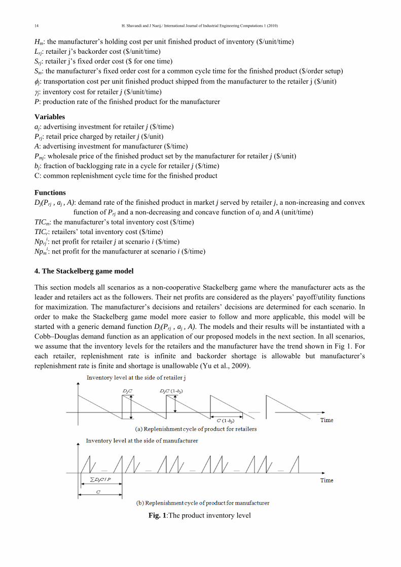
(2) Based on the VMI strategy, the supplier is responsible for the chain wide two-echelon inventories which include the finished product’s inventories at the retailers’ sides and the supplier’s side depicted by Fig. 1. A common replenishment cycle policy is adopted by the supplier to manage the inventories of the product. Each retailer pays the inventory cost based on the demand rate to the supplier.

(3) There is a leader-follower relationship between the supplier (manufacturer) and the retailers. According to the VMI strategy, all the necessary market information of the retailers are available for the supplier and the supplier completely benefit to better serve the retailers.

3.2. Notations Indices n: number of retailers j: index of the retailers Parameters Cm: manufacturing cost for per unit finished product ($/unit) Hrj: retailer j’s holding cost ($/unit/time)


14

Hm: the manufacturer’s holding cost per unit finished product of inventory ($/unit/time) Lrj: retailer j’s backorder cost ($/unit/time) Srj: retailer j’s fixed order cost ($ for one time) Sm: the manufacturer’s fixed order cost for a common cycle time for the finished product ($/order setup) φj: transportation cost per unit finished product shipped from the manufacturer to the retailer j ($/unit) γj: inventory cost for retailer j ($/unit/time) P: production rate of the finished product for the manufacturer

Variables aj: advertising investment for retailer j ($/time) Prj: retail price charged by retailer j ($/unit) A: advertising investment for manufacturer ($/time) Pmj: wholesale price of the finished product set by the manufacturer for retailer j ($/unit) bj: fraction of backlogging rate in a cycle for retailer j ($/time) C: common replenishment cycle time for the finished product

Functions Dj(Prj , aj , A): demand rate of the finished product in market j served by retailer j, a non-increasing and convex

function of Prj and a non-decreasing and concave function of aj and A (unit/time) TICm: the manufacturer’s total inventory cost ($/time) TICr: retailers’ total inventory cost ($/time) Nprj

i: net profit for retailer j at scenario i ($/time) Npm

i: net profit for the manufacturer at scenario i ($/time) 4. The Stackelberg game model

This section models all scenarios as a non-cooperative Stackelberg game where the manufacturer acts as the leader and retailers act as the followers. Their net profits are considered as the players’ payoff/utility functions for maximization. The manufacturer’s decisions and retailers’ decisions are determined for each scenario. In order to make the Stackelberg game model more easier to follow and more applicable, this model will be started with a generic demand function Dj(Prj , aj , A). The models and their results will be instantiated with a Cobb–Douglas demand function as an application of our proposed models in the next section. In all scenarios, we assume that the inventory levels for the retailers and the manufacturer have the trend shown in Fig 1. For each retailer, replenishment rate is infinite and backorder shortage is allowable but manufacturer’s replenishment rate is finite and shortage is unallowable (Yu et al., 2009).

Fig. 1:The product inventory level


15

4.1. Scenario 1 In the first scenario, the inventory policy is an information-asymmetric VMI and the producer provides a single product at the same wholesale price to multiple retailers (Pm). The payoff function (net profit) for each player is equal to its revenue minus its total cost. 4.1.1. Net profit of each retailer The revenue of retailer j is Prj Dj(Prj , aj , A). Its cost includes three components: product cost Pm Dj(Prj , aj , A), advertising investment aj, and inventory cost jγ Dj(Prj , aj , A) is proportion to its demand. The order, backorder

and holding costs do not appear in retailer’s cost formula since supplier is responsible for it based on VMI rules. The net profit for retailer j can be given by

, , (1)

4.1.2. Net profit of manufacturer The total revenue for the manufacturer comes from the selling of the product to its retailers at wholesale price Pm given by (1). The total cost also consists of manufacturer's inventory cost (TICm), the retailers’ inventory cost (TICr) and the advertising investment (A). Based on Fig. 1, in a supply chain, it is not unusual for the manufacturer to assume a common replenishment period for all its retailers (Banerjee & Burton, 1994; Chakravarty & Goyal, 1986; Chen & Chen, 2005; Mitra & Chatterjee, 2004; Viswanathan & Piplani, 2001; Woo et al., 2001). Therefore we have,

1 ∑ , ,2 ∑ , , . (2)

The first term in Eq. (2) is the sum of the setup and the holding cost of manufacturer’s side and the second term is the production cost. Retailers’ inventory cost includes order cost, holding cost, backorder cost and transportation cost.

1 , , 12

, ,2

, , .

(3)

Therefore, the net profit of the manufacturer is computed as follows, ∑ , , . (4)

The first proposed Stackelberg game model is formulated as follows,

, … , , , , , , (4)

subject to

, , , (5)

0 1 , 1, … , (6)

, , 0. (7)


16

and

, , , , 1, … , (8)

subject to

, 1, … , (9)

, 0 . 1, … , (10)

Eqs. (4) and (8) are the objective functions of the manufacturer and its retailers, respectively. Constraint (5) is the production capacity constraint an constraints (6) demonstrate the lower and the upper bounds for retailer’s backorder. The basic feasible condition of the retailers is explained in constraints (9). Finally, the decision variables are defined by the remaining constraints. 4.1.3. The Stackelberg equilibrium The Stackelberg equilibrium is obtained using a backward procedure. Based on this procedure, the followers’ (retailer) problem must be solved first to get the response functions of the leader’s (manufacturer) decisions. In the next step, the manufacturer’s decision problem is solved by attending all possible reactions of the followers to maximize the net profit. Every follower’s optimal response can be determined by considering the manufacturer’s decisions as its input parameters. Finally, the leader finds its optimal decision by assuming that the followers take the optimal response. In our model, the best response functions established analytically for the retailers since they are involved and we are faced with relatively large number of variables. Retailers’ best response functions By taking the first derivative of Eq. (8) with respect to aj, we have

, , , 1 , 1, … , . (11)

Solving , 0 yields the critical point of the equation with Dj(Prj , aj , A) as non-decreasing and

concave function of aj. Since , 0, only one critical point exists and it is a function of (Prj,A).

The critical point is the optimal solution of retailer j for any given (Prj,A) denoted as

, , 1, … , . (12)

Taking the first derivative of Nprj (Prj, aj*) with respect to Prj yields,

,

, ,, , , , ,

0.

(13)

We get the optimal solution Prj* by solving Eq. (13). This equation has at least one critical point otherwise,

Nprj1 (Prj, aj*) will be a monotone function of Prj. Based on a given specific demand function, Eqs. (12) and

(13) are the best response functions for retailer j.


17

Manufacturer’s decision problem The manufacturer determines decision variables by Eqs. (4)-(7) and considering retailers’ best response functions. , … , , , , is a concave function of bj for any other given variables since

,…, , , , 0. Taking the first derivate of Eq. (4) respect to bj yields,

, 1, … , . (14)

Using Eqs. (12)-(14) in Eq. (4) and taking the first derivative respect to C, yields the optimal value of C* as follows,

∑ , (15)

where

∑ , , , , . (16)

Since , , ∑ 0, then , , is a concave function of C for any given Pm and A. Therefore, the manufacturer’s net profit becomes a function of variables Pm and A which yields to the following optimization problem.

, , , , , (17)

subject to

, , , (18)

, 0. (19)

As we can see, there are only two continuous variables left and therefore, the Kuhn–Tucker conditions (KKT) can be used to calculate the optimal solutions. Suppose λ be the Lagrange multiplier, then we have,

, , , ∑ , , . (20)

Then the KKT conditions for the model is follows,

, ∑ , ,0 , (21)

, ∑ , ,0, (22)

∑ , , 0. (23)

Therefore we can find the Stackelberg game equilibrium from the all solutions satisfying all optimal conditions under any given specific demand function Dj(Prj , aj , A).


18

4.2. Scenario 2 In the second scenario, like the first scenario, the inventory policy is an information-asymmetric VMI but the producer provides a single product at the wholesale price Pmj to retailer j. 4.2.1. Net profit of each retailer The difference between Net profit of each retailer at the first and the second scenarios is in product cost. In the other word, for the second scenario retailer j’s product cost is Pmj Dj(Prj , aj , A). Then

, , . (24)

4.2.2. Net profit of manufacturer The Net profit of manufacturer is as follows,

∑ , , . (25)

where TICm obtain from Eq. (2) and

1 , , 12

, ,2 , , . (26)

Therefore, we can formulate the model for the second scenario as a Stackelberg game model as follows,

, … , , , , , … , , , (27)

subject to Eqs. (5)-(6)

, , 0 , 1, … , (28)

and

, , , , 1, … , (29)

subject to Eq. (10)

, 1, … , (30)

4.2.3. The Stackelberg equilibrium The Stackelberg equilibrium has the same form as the one given in section 4.1.3. So, the retailer j’s best response functions are

, , ,1 0 , 1, … , (31)

, , , , , , , ,0. (32)

Thus, we get the optimal solution Prj* and aj

* by solving Eqs. (32) and (31), respectively. The manufacturer’s decision variables are obtained by Eqs. (5), (6), (27), (28) and the retailers’ best response functions are also obtained from Eqs. (31) and (32). Then, the optimal value of bj is

, 1, … , (33)


19

Eqs. (15), (16) and (33) give the optimal value of C*. Therefore, the manufacturer’s net profit is as follows,

, … , , , , , , (34)

subject to

, , , (35)

, , … , 0. (36)

TICm and TICr are determined from Eqs. (2) and (26), respectively and Prj*, aj

* and bj* are resulted from Eqs.

(31)-(33). Because the above model is continues model of n+1 variables, then the KKT conditions can be used to calculate the optimal solutions. Suppose λ be Lagrange multiplier, thus,

, ∑ , ,0 , 1, … , (37)

, ∑ , ,0, (38)

, , 0. (39)

Therefore, the Stackelberg game equilibrium can be computed from the solution of the equations Eq. (37) to Eq. (39) under any given specific demand function. 4.3. Scenario 3 In the third scenario, unlike the two previous scenarios, the inventory policy is a periodic inventory system for each side of supply chain. In the other words, the manufacturer, as supplier, produces a product under independent periodic inventory systems (without commitment for managing its retailers’ ordering and inventory levels) and sells it at the same wholesale price to all retailers (Pm). Each retailer by considering his own cost and demand uses the ordering periodic system relevant to manufacturer’s production cycle. Therefore, the manufacturer and each retailer pay themselves the total inventory cost, separately. 4.3.1. Net profit of each retailer The revenue of retailer j is Prj Dj(Prj , aj , A). Its cost includes three components; product cost Pm Dj(Prj , aj , A), advertising investment aj, and total inventory cost TICr involved ordering cost, holding cost and transporting cost which are calculated as follows,

1 , , 12

, ,2

, , ,

1, … ,

(40)

Note that retailers need to coordinate with supplier (manufacturer) to adopt their replenishment cycle with manufacturer’s production cycle. Therefore, C in Eq. (40) is an input parameter and the net profit for the retailer j can be given by


20

, , , , . (41)

4.3.2. Net profit of manufacturer The total net revenue for the manufacturer comes from the selling of the product to its retailers at wholesale price Pm minus the associated inventory cost (TICm) and the advertising investment (A) costs as follows,

, , ∑ , , , (42)

where, TICm is obtained from Eq. (2). Therefore, the Stackelberg equilibrium model is formulated as follows,

, , , , (43)

subject to Eqs. (5) and (7) and

, , , , , 1, … , (44)

subject to Eqs. (6), (9) and (10)

4.3.3. The Stackelberg equilibrium To determine the Stackelberg equilibrium we repeat the same operations explained in section 4.1.3. Retailers’ best response functions

Let , , 0 and since Dj (Prj, aj, A) is a non-decreasing and concave function of aj. Thus

, , , ,1 0 , 1, … , (45)

Because , , 0, only one critical point exists and it is a function of (bj, Prj, A). The critical point

is the optimal solution of retailer j for any given (bj, Prj, A), and denoted as,

, , , 1, … , (46)

The optimal solution of Prj* is computed as follows,

, ,

, ,, , , , ,

0

(47)

As mentioned in section 4.1.3, this equation has at least one critical point. Therefore Eqs. (46) and (47) are the best response functions for retailer j. Finally, from setting the result to zero for the first derivative with respect to bj of Eq. (44), the optimal value of bj can be obtained as follows,


21

, ,, , 1 , , 0

, 1, … ,

(48)

The above critical point is the optimal solution because,

, ,, , , , 0

Manufacturer’s decision problem The manufacturer’s decision variables are determined by Eq. (44) and we have the retailers’ best response functions , , . , , is a concave function of C for any other given variables since

, , 0. Therefore, from setting the result to zero for the first derivative with respect to C of Eq. (44), the optimal value of C* can be obtained as follows,

2∑ , ,

(49)

Therefore, the manufacturer’s net profit becomes a function of variables Pm and A:

, , , , (50)

subject to

∑ , , , (51)

, 0. (52)

Therefore, the KKT conditions are as follows,

, ∑ , ,0 , (53)

, ∑ , ,0, (54)

∑ , , 0. (55)

The Stackelberg game equilibrium is determined by solving Eq. (53) to Eq. (55). 4.4. Scenario 4 For the fourth scenario, like the third scenario, the inventory policy is a periodic inventory system for each side of the supply chain but the manufacturer produces and sells a single product at the wholesale price Pmj to retailer j. 4.4.1. Net profit of each retailer The main difference between the net profit for each retailer in the third and the fourth scenarios is in product cost. In the other word, for the fourth scenario the retailer j’s product cost is Pmj Dj(Prj , aj , A). Therefore we have,


22

, , , , (56)

where

1 , , 12

, ,2

, , , 1, … ,

(57)

4.4.2. Net profit of manufacturer The Net profit of manufacturer is

, , , … , , , (58)

where, TICm is obtained from Eq. (2). Therefore, the Stackelberg game model for this scenario is as follows, , , , … , ∑ , , , (59)

subject to Eqs. (5) and (28)

and

, , , , , 1, … , (60)

subject to Eqs. (6), (10) and (30),

where TICm and TICr are determined by Eqs. (2) and (57), respectively. 4.4.3. The Stackelberg equilibrium Similar to what we explained in previous sections, the retailer j’s best response functions are as follows,

, , , ,1 0 , 1, … , (61)

, ,

, ,, , , , ,

0 (62)

, ,

, , 1 , , 0

, 1, … ,

(63)

Thus, we get the optimal solution bj*, Prj

* and aj* by solving Eqs. (63), (62) and (61), respectively.

From solving Eqs. (5), (6), (27), (28) and by considering retailers’ best response functions from Eqs. (61), (62) and (63), the manufacturer’s decision variables are calculated as follows,


23

2∑ , ,

(64)

Using Eqs. (61)-(64), the manufacturer’s net profit is calculated as follows,

, … , , , , , (65)

subject to

, , , (66)

, , … , 0 (67)

Assuming λ as the Lagrange multiplier, the KKT conditions are as follows,

, ∑ , ,0 , 1, … , (68)

, ∑ , ,0, (69)

∑ , , 0. (70)

Therefore, the Stackelberg game equilibrium can be calculated from the solution of Eqs (68)-(70). 4.5. Solution algorithm The previous analysis for all scenarios can be summarized using the steps of the following algorithm to find the equilibrium point of the Stackelberg game model. Algorithm Step1: Calculate the manufacturer’s decision variables with respect to retailers’ best response functions. Step2: Based on the optimal manufacturer’s decision variables, obtained from step1, calculate the optimal

retailers’ best response functions. Step3: Consider the results of step1 and step2, calculate the net profit of the manufacturer and the retailers. 5. Numerical example

In order to demonstrate the implementations of the proposed method of this paper and analyze the results of our methodology we use a numerical example. The purpose of this numerical example is to demonstrate the results of the proposed Stackelberg game and its solution algorithm and to present meaningful managerial insights from studying different scenarios. For this purpose, we have selected a Cobb–Douglas demand function to specify and validate our proposed models. A Cobb–Douglas function is defined as ∏ . It explains the relationship between an output (f) and substitutable inputs (xi) with given elasticity parameters ει, i=1,…,n. It was introduced by Knut Wicksell (1851–1926), and tested against statistical evidence by Cobb and Douglas (1928). In this paper, the product demand of retailer j, Dj(Prj , aj , A) for j=1,..,n is dependent on its retail price (Prj), the manufacturer’s advertising investment (A), and the retailer i’s advertising investment (aj) where their relationship can be well introduced by the Cobb–Douglas demand function as:


24

, , , 1, … , (71)

where Kj is a positive constant representing the market scale of retailer j; αj; βj; and ρj represent the elasticity parameters of aj, A and Prj (Yu et al, 2009). Because Dj(Prj , aj , A) is a non-decreasing and concave function of aj, then we have,

, , 0,

, , 1 0,

(71)

which means 0 < αj <1. Similarly, we can get 0 < βj <1 and ρj >0. Since Prj is positive and based on the optimal value of Prj in all scenarios we can conclude that ρj >1. To set game parameters reasonably, they need to be selected carefully based on investigating suggestions and practices given by other researchers (Lee, So, & Tang, 2000; Woo et al., 2001; Yu et al., 2009), and some properties of the Cobb–Douglas function (70) originally used in supply chain practices. For examples, the holding cost per unit finished product at a retailer side must be higher than the manufacturer’s side. The backorder cost per unit product also must be higher than the holding cost per unit product (Lee, So, & Tang, 2000; Woo et al., 2001; Yu et al., 2009). After careful considerations, suitable input parameters of the example are given in Table 1. As an illustration, the case of two retailers is discussed. The unit time is one year and the monetary unit is US dollar. The optimal decisions for the retailers and the manufacturer for all scenarios are presented in Table 2.From the results in table 2, the manufacturer gains the maximum profit in the first scenario unlike the retailers 1 and 2 whose best scenarios are three and four, respectively. From manufacturer’s point of view, we can understand that having VMI policy and offering uniform pricing is the best strategy, while from retailers’ point of view, the independent periodic inventory policy is the best policy. 6. Sensitivity analysis

Sensitivity analysis has been performed for market-related parameters (α, β, λ). In this section, we study the effects of each parameter on the manufacturer’s net profit and retailers’ net profit and compare these effects for all scenarios. Table1 Input parameters λ2 λ1 β2 β1 α2 α1 K2 K1 P I Hm Sm Cm φ2 φ1 Sr2 Sr1 Lr2 Lr1 N 1.4 1.3 0.39 0.39 0.41 .43 350 350 50000 0.2 4 200 20 11 10 110 100 520 500 2 Table 2 Optimal decisions for the retailers and the manufacturer for all scenarios

Scenario

Pmj Prj aj(106) A(106) C

bj Dj Nprj(106) Npm

(106) 1 2 1 2 1 2 1 2 1 2 1 2

1 74.13 - 364.54 290.94 2.058 0.439 0.807 0.049 0.029 0.028 17072 5149 2.729 0.621 0.374

2 77.48 68.06 379.1 269.7 2.003 0.459 0.799 0.049 0.030 0.026 15977 5810 2.656 0.649 0.370

3 69.74 - 352.6 288.3 2.088 0.44 0.803 0.240 0.027 0.026 17899 5210 2.767 0.633 0.343

4 71.63 63.94 361.11 267.63 2.068 0.464 0.807 0.244 0.028 0.024 17315 5921 2.741 0.667 0.344


25

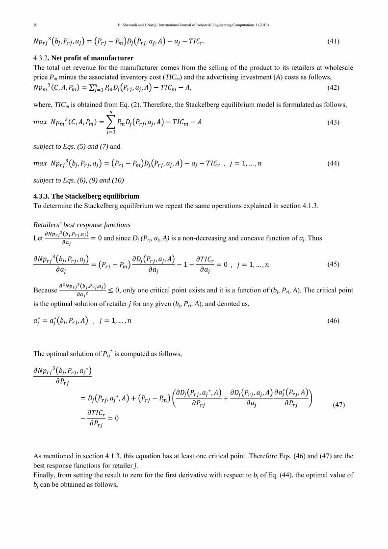
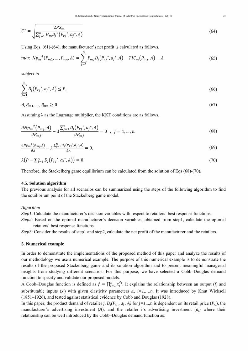
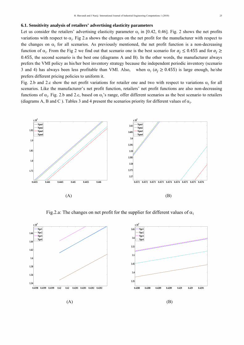
6.1. Sensitivity analysis of retailers’ advertising elasticity parameters Let us consider the retailers’ advertising elasticity parameter αj in [0.42, 0.46]. Fig. 2 shows the net profits variations with respect to αj. Fig 2.a shows the changes on the net profit for the manufacturer with respect to the changes on αj for all scenarios. As previously mentioned, the net profit function is a non-decreasing function of αj. From the Fig 2 we find out that scenario one is the best scenario for 0.455 and for 0.455, the second scenario is the best one (diagrams A and B). In the other words, the manufacturer always prefers the VMI policy as his/her best inventory strategy because the independent periodic inventory (scenario 3 and 4) has always been less profitable than VMI. Also, when αj ( 0.455) is large enough, he/she prefers different pricing policies to uniform it. Fig. 2.b and 2.c show the net profit variations for retailer one and two with respect to variations αj for all scenarios. Like the manufacturer’s net profit function, retailers’ net profit functions are also non-decreasing functions of αj. Fig. 2.b and 2.c, based on αj’s range, offer different scenarios as the best scenario to retailers (diagrams A, B and C ). Tables 3 and 4 present the scenarios priority for different values of αj.

(A) (B)

(A) (B)

0.4435 0.444 0.4445 0.445 0.4455 0.446

1.75

1.8

1.85

1.9

1.95

x 106

Npm1Npm2Npm3Npm4

0.4572 0.4572 0.4573 0.4573 0.4574 0.4574 0.4575 0.4575 0.4576

3.57

3.575

3.58

3.585

3.59

3.595

3.6

3.605

3.61

x 106

Npm1Npm2Npm3Npm4

0.4198 0.4199 0.4199 0.42 0.42 0.4201 0.4201 0.4202 0.4202

1.54

1.56

1.58

1.6

1.62

1.64

1.66

x 106

Npr1Npr2Npr3Npr4

0.4288 0.4288 0.4289 0.4289 0.429 0.429 0.4291

3.35

3.4

3.45

3.5

3.55

3.6

3.65x 106

Npr1Npr2Npr3Npr4

Fig.2.a: The changes on net profit for the supplier for different values of αj


26

(C)

(A) (B)

(C)

0.453 0.4535 0.454 0.4545 0.455 0.4555

1.03

1.04

1.05

1.06

1.07

1.08

1.09

1.1

1.11

x 107

Npr1Npr2Npr3Npr4

0.4215 0.422 0.4225 0.423 0.4235 0.424

7

7.5

8

8.5

9

9.5

x 105

Npr1Npr2Npr3Npr4

0.442 0.4425 0.443 0.4435 0.444 0.4445

2.4

2.45

2.5

2.55

2.6

x 106

Npr1Npr2Npr3Npr4

0.452 0.453 0.454 0.455 0.456 0.457 0.458

3.2

3.3

3.4

3.5

3.6

3.7

x 106

Npr1Npr2Npr3Npr4

Fig.2.b: The change on the first net profit for all scenarios

Fig.2.c: The changes on the second retailer's net profit


27

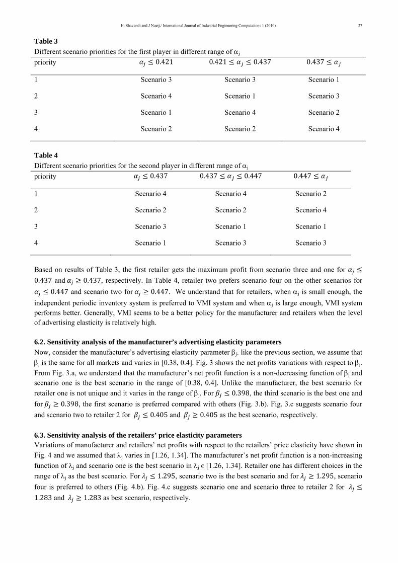
Table 3 Different scenario priorities for the first player in different range of αj priority 0.421 0.421 0.437 0.437

1 Scenario 3 Scenario 3 Scenario 1




Table 4 Different scenario priorities for the second player in different range of αj priority 0.437 0.437 0.447 0.447





Based on results of Table 3, the first retailer gets the maximum profit from scenario three and one for 0.437 and 0.437, respectively. In Table 4, retailer two prefers scenario four on the other scenarios for

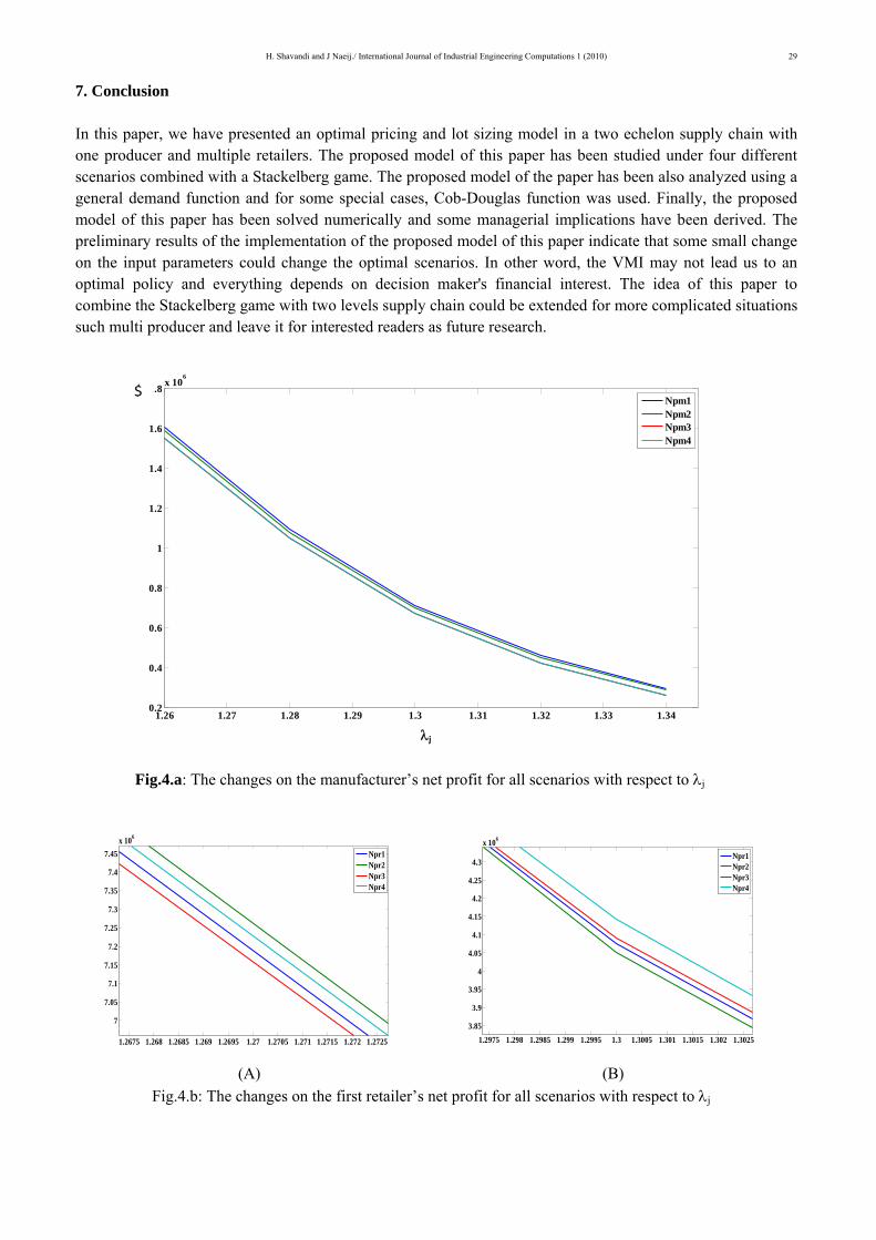
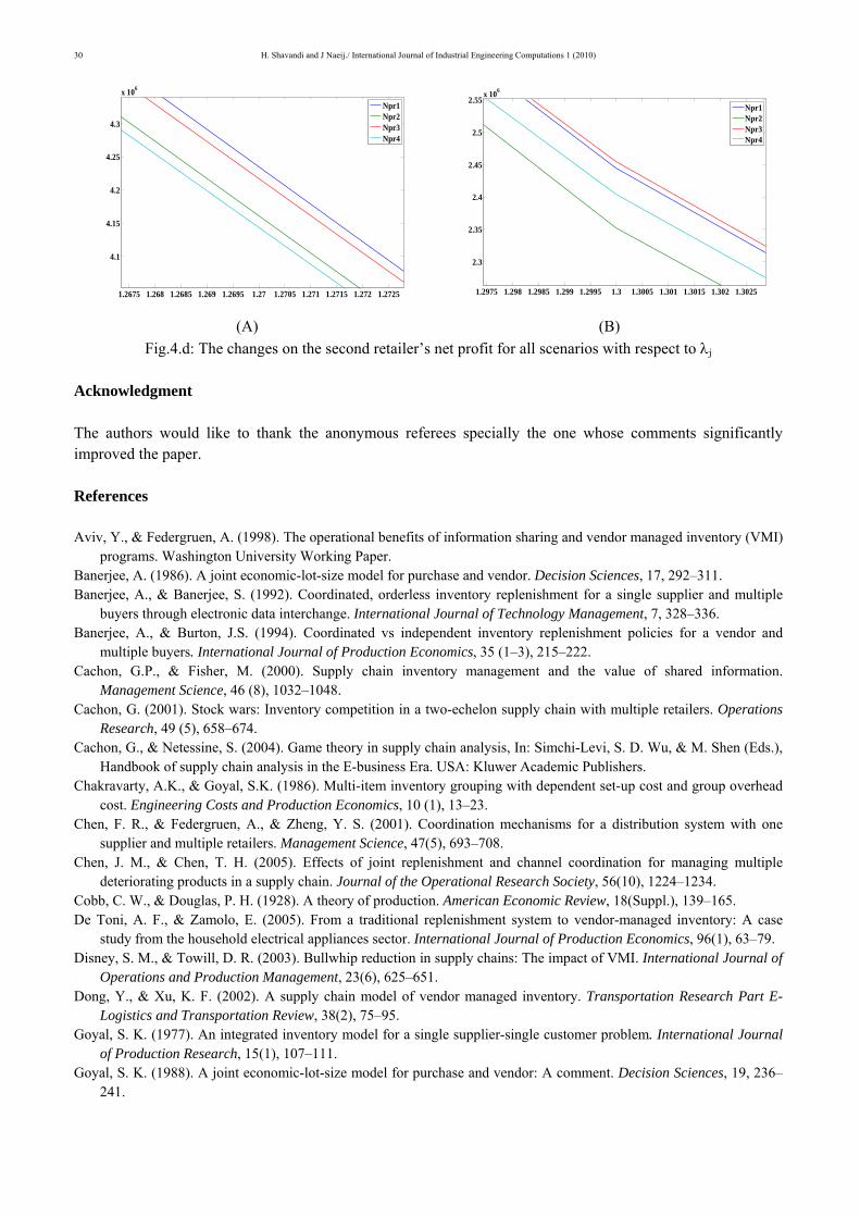
0.447 and scenario two for 0.447. We understand that for retailers, when αj is small enough, the independent periodic inventory system is preferred to VMI system and when αj is large enough, VMI system performs better. Generally, VMI seems to be a better policy for the manufacturer and retailers when the level of advertising elasticity is relatively high. 6.2. Sensitivity analysis of the manufacturer’s advertising elasticity parameters Now, consider the manufacturer’s advertising elasticity parameter βj. like the previous section, we assume that βj is the same for all markets and varies in [0.38, 0.4]. Fig. 3 shows the net profits variations with respect to βj. From Fig. 3.a, we understand that the manufacturer’s net profit function is a non-decreasing function of βj and scenario one is the best scenario in the range of [0.38, 0.4]. Unlike the manufacturer, the best scenario for retailer one is not unique and it varies in the range of βj. For 0.398, the third scenario is the best one and for 0.398, the first scenario is preferred compared with others (Fig. 3.b). Fig. 3.c suggests scenario four and scenario two to retailer 2 for 0.405 and 0.405 as the best scenario, respectively. 6.3. Sensitivity analysis of the retailers’ price elasticity parameters Variations of manufacturer and retailers’ net profits with respect to the retailers’ price elasticity have shown in Fig. 4 and we assumed that λj varies in [1.26, 1.34]. The manufacturer’s net profit function is a non-increasing function of λj and scenario one is the best scenario in λj є [1.26, 1.34]. Retailer one has different choices in the range of λj as the best scenario. For 1.295, scenario two is the best scenario and for 1.295, scenario four is preferred to others (Fig. 4.b). Fig. 4.c suggests scenario one and scenario three to retailer 2 for 1.283 and 1.283 as best scenario, respectively.


28

Fig.3.a: The changes on manufacturer’s net profit for all scenarios with respect to βj

(A) (B) Fig.3.b: The changes on the first retailer's net profit for all scenarios with respect to βj

Fig.3.c: The changes on the second retailer's net profit for all scenarios with respect to βj

0.38 0.385 0.39 0.395 0.41

2

3

4

5

6

7

8

9 x 105

Npm1Npm2Npm3Npm4

0.3944 0.3946 0.3948 0.395 0.3952 0.3954 0.3956

3.95

4

4.05

4.1

4.15

4.2

4.25

x 106

Npr1Npr2Npr3Npr4

0.3993 0.3994 0.3995 0.3996 0.3997 0.3998 0.3999 0.4

6

6.02

6.04

6.06

6.08

6.1

6.12

x 106

Npr1Npr2Npr3Npr4

0.398 0.3985 0.399 0.3995 0.4 0.4005 0.401

1.28

1.3

1.32

1.34

1.36

1.38

1.4

1.42

1.44

1.46

1.48x 106

β

Npr1Npr2Npr3Npr4

βj

$


29

7. Conclusion In this paper, we have presented an optimal pricing and lot sizing model in a two echelon supply chain with one producer and multiple retailers. The proposed model of this paper has been studied under four different scenarios combined with a Stackelberg game. The proposed model of the paper has been also analyzed using a general demand function and for some special cases, Cob-Douglas function was used. Finally, the proposed model of this paper has been solved numerically and some managerial implications have been derived. The preliminary results of the implementation of the proposed model of this paper indicate that some small change on the input parameters could change the optimal scenarios. In other word, the VMI may not lead us to an optimal policy and everything depends on decision maker's financial interest. The idea of this paper to combine the Stackelberg game with two levels supply chain could be extended for more complicated situations such multi producer and leave it for interested readers as future research.

Fig.4.a: The changes on the manufacturer’s net profit for all scenarios with respect to λj

(A) (B) Fig.4.b: The changes on the first retailer’s net profit for all scenarios with respect to λj

1.26 1.27 1.28 1.29 1.3 1.31 1.32 1.33 1.340.2

0.4

0.6

0.8

1

1.2

1.4

1.6

1.8 x 106

Npm1Npm2Npm3Npm4

1.2675 1.268 1.2685 1.269 1.2695 1.27 1.2705 1.271 1.2715 1.272 1.2725

7

7.05

7.1

7.15

7.2

7.25

7.3

7.35

7.4

7.45x 106

Npr1Npr2Npr3Npr4

1.2975 1.298 1.2985 1.299 1.2995 1.3 1.3005 1.301 1.3015 1.302 1.30253.85

3.9

3.95

4

4.05

4.1

4.15

4.2

4.25

4.3

x 106

Npr1Npr2Npr3Npr4

λj

$


30

(A) (B) Fig.4.d: The changes on the second retailer’s net profit for all scenarios with respect to λj

Acknowledgment The authors would like to thank the anonymous referees specially the one whose comments significantly improved the paper. References Aviv, Y., & Federgruen, A. (1998). The operational benefits of information sharing and vendor managed inventory (VMI)

programs. Washington University Working Paper. Banerjee, A. (1986). A joint economic-lot-size model for purchase and vendor. Decision Sciences, 17, 292–311. Banerjee, A., & Banerjee, S. (1992). Coordinated, orderless inventory replenishment for a single supplier and multiple

buyers through electronic data interchange. International Journal of Technology Management, 7, 328–336. Banerjee, A., & Burton, J.S. (1994). Coordinated vs independent inventory replenishment policies for a vendor and

multiple buyers. International Journal of Production Economics, 35 (1–3), 215–222. Cachon, G.P., & Fisher, M. (2000). Supply chain inventory management and the value of shared information.

Management Science, 46 (8), 1032–1048. Cachon, G. (2001). Stock wars: Inventory competition in a two-echelon supply chain with multiple retailers. Operations

Research, 49 (5), 658–674. Cachon, G., & Netessine, S. (2004). Game theory in supply chain analysis, In: Simchi-Levi, S. D. Wu, & M. Shen (Eds.),

Handbook of supply chain analysis in the E-business Era. USA: Kluwer Academic Publishers. Chakravarty, A.K., & Goyal, S.K. (1986). Multi-item inventory grouping with dependent set-up cost and group overhead

cost. Engineering Costs and Production Economics, 10 (1), 13–23. Chen, F. R., & Federgruen, A., & Zheng, Y. S. (2001). Coordination mechanisms for a distribution system with one

supplier and multiple retailers. Management Science, 47(5), 693–708. Chen, J. M., & Chen, T. H. (2005). Effects of joint replenishment and channel coordination for managing multiple

deteriorating products in a supply chain. Journal of the Operational Research Society, 56(10), 1224–1234. Cobb, C. W., & Douglas, P. H. (1928). A theory of production. American Economic Review, 18(Suppl.), 139–165. De Toni, A. F., & Zamolo, E. (2005). From a traditional replenishment system to vendor-managed inventory: A case

study from the household electrical appliances sector. International Journal of Production Economics, 96(1), 63–79. Disney, S. M., & Towill, D. R. (2003). Bullwhip reduction in supply chains: The impact of VMI. International Journal of

Operations and Production Management, 23(6), 625–651. Dong, Y., & Xu, K. F. (2002). A supply chain model of vendor managed inventory. Transportation Research Part E-

Logistics and Transportation Review, 38(2), 75–95. Goyal, S. K. (1977). An integrated inventory model for a single supplier-single customer problem. International Journal

of Production Research, 15(1), 107–111. Goyal, S. K. (1988). A joint economic-lot-size model for purchase and vendor: A comment. Decision Sciences, 19, 236–

241.

1.2675 1.268 1.2685 1.269 1.2695 1.27 1.2705 1.271 1.2715 1.272 1.2725

4.1

4.15

4.2

4.25

4.3

x 106

Npr1Npr2Npr3Npr4

1.2975 1.298 1.2985 1.299 1.2995 1.3 1.3005 1.301 1.3015 1.302 1.3025

2.3

2.35

2.4

2.45

2.5

2.55x 106

Npr1Npr2Npr3Npr4


31

Goyal, S. K., & Gunasekaran, A. (1995). An integrated production-inventory marketing model for deteriorating items. Computers & Industrial Engineering, 28(4), 755–762.

Huang, Z. M., & Li, S. X. (2001). Co-op advertising models in manufacturer–retailer supply chains: A game theory approach. European Journal of Operational Research, 135(3), 527–544.

Kohli, R., & Park, H. (1994). Coordinating buyer–seller transactions across multiple products. Management Science, 40(9), 45–50.

Kotler, P. (1971). In market decision making: A model building approach. New York: Holt Rinchart Winstion. Ladany, S., & Sternleib, A. (1974). The interaction of economic ordering quantities and marketing policies. AIIE

Transactions, 6, 35–40. Lal, R., & Staelin, R. (1984). An approach for developing an optimal discount pricing policy. Management Science, 30,

1524–1539. Lau, A. H. L., & Lau, H. S. (2004). Some two-echelon supply-chain games: Improving from deterministic-symmetric-

information to stochastic asymmetric-information models. European Journal of Operational Research, 161(1), 203–223.

Lau, A. H. L., Lau, H. S., & Zhou, Y. W. (2007). A stochastic and asymmetric-information framework for a dominant-manufacturer supply chain. European Journal of Operational Research, 176(1), 295–316.

Lee, H. L., So, K. C., & Tang, C. S. (2000). The value of information sharing in a two level supply chain. Management Science, 46(5), 626–643.

Liou, Y. C., Schaible, S., & Yao, J. C. (2006). Supply chain inventory management via a Stackelberg equilibrium. Journal of Industrial and Management Optimization, 2(1), 81–94.

Lu, L. (1995). A one-vendor multi-buyer integrated inventory model. European Journal of Operational Research, 81, 312–323.

Mitra, S., & Chatterjee, A. K. (2004). Leveraging information in multi-echelon inventory systems. European Journal of Operational Research, 152(1), 263–280.

Monahan, J. P. (1984). A quantity discount pricing model to increase vendor profits. Management Science, 30(6), 720–726.

Munson, C. L., & Rosenblatt, M. J. (2001). Coordinating a three-level supply chain with quantity discounts. IIE Transactions, 33(5), 371–384.

Qin, Y., Tang, H., & Guo, C. (2007). Channel coordination and volume discounts with price-sensitive demand. International Journal of Production Economics, 105(1), 43–53.

Rosenblatt, M. J., & Lee, H. L. (1985). Improving profitability with quantity discounts under fixed demand. IIE Transactions, 17, 388–395.

Roslow, S., Laskey, H. A., & Nicholls, J. A. F. (1993). The enigma of cooperative advertising. Journal of Business & Industrial Marketing, 8, 70–79.

Rusdiansyah, A., & Tsao, D. B. (2005). An integrated model of the periodic delivery problems for vending-machine supply chains. Journal of Food Engineering, 70(3), 421–434.

Samuelson, P. (1947). Foundations of Economic Analysis. Harvard University Press, Cambridge, MA. Simchi-Livi, D., & Kaminsky, P., Simchi-Livi, E. (2000). Designing and managing the supply chain-concepts strategies

and case studies. Singapore: McGraw-Hill. Subramanyam, S., & Kumaraswamy, S. (1981). EOQ formula under varying marketing polices and conditions. AIIE

Transactions, 13, 312–314. Viswanathan, S., & Piplani, R. (2001). Coordinating supply chain inventories through common replenishment epochs.

European Journal of Operational Research, 129 (2), 277–286. Vives, X. (1990). Nash equilibrium with strategic complementarities. Journal of Mathematical Economics, 19, 305–321. Wang, Q. N. (2002). Determination of suppliers’ optimal quantity discount schedules with heterogeneous buyers. Naval

Research Logistics, 49(1), 46–59. Weng, Z. K. (1995). Channel coordination and quantity discounts. Management Science, 41(9), 1509–1522. Woo, Y. Y., Hsu, S. L., & Wu, S. S. (2001). An integrated inventory model for a single vendor and multiple buyers with

ordering cost reduction. International Journal of Production Economics, 73(3), 203–215. Yao, Y. L., Evers, P. T., & Dresner, M. E. (2007). Supply chain integration in vendor managed inventory. Decision

Support Systems, 43(2), 663–674. Yao, Y., Dong, Y., & Dresner, M. (2010). Managing supply chain backorders under vendor managed inventory: An

incentive approach and empirical analysis, European Journal of Operational Research, 203(2), 350-359.


32

Yu, Y. G., & Liang, L. (2004). An integrated vendor-managed-inventory model for end product being deteriorating item. Chinese Journal of Management Science, 12, 32–37. in Chinese.

Yu, Y., Chu, F., & Chen, H. (2009). A Stackelberg game and its improvement in a VMI system with a manufacturing vendor. European Journal of Operational Research, 192, 929–948.

Yu, Y., Huang, G.Q., & Liang, L. (2009). Stackelberg game-theoretic model for optimizing advertising, pricing and inventory policies in vendor managed inventory (VMI) production supply chains. Computers & Industrial Engineering,

57, 368–382, Zhang, T., Liang, L., Yu, Y., & Yu, Y. (2007). An integrated vendor-managed inventory model for a two-echelon system

with order cost reduction. International Journal of Production Economics, 109 (1–2), 241–253.

international journal of indus trial engineering...

Documents