International Journal of Solids and Structures 174–175 (2019) 53–68

Contents lists available at ScienceDirect

International Journal of Solids and Structures

journal homepage: www.elsevier.com/locate/ijsolstr

The multiplicative deformation split for shells with application to

growth, chemical swelling, thermoelasticity, viscoelasticity and

elastoplasticity

Roger A. Sauer a , ∗, Reza Ghaffari a , Anurag Gupta

b

a Aachen Institute for Advanced Study in Computational Engineering Science (AICES), RWTH Aachen University, Templergraben 55, Aachen 52056, Germany b Department of Mechanical Engineering, Indian Institute of Technology Kanpur, UP 208016, India

a r t i c l e i n f o

Article history:

Received 3 December 2018

Revised 20 May 2019

Accepted 4 June 2019

Available online 7 June 2019

Keywords:

Curvilinear coordinates

Inelastic shells

Irreversible thermodynamics

Multiplicative decomposition

Nonlinear shell theory

Kirchhoff–Love kinematics

a b s t r a c t

This work presents a general unified theory for coupled nonlinear elastic and inelastic deformations of

curved thin shells. The coupling is based on a multiplicative decomposition of the surface deformation

gradient. The kinematics of this decomposition is examined in detail. In particular, the dependency of

various kinematical quantities, such as area change and curvature, on the elastic and inelastic strains is

discussed. This is essential for the development of general constitutive models. In order to fully explore

the coupling between elastic and different inelastic deformations, the surface balance laws for mass, mo-

mentum, energy and entropy are examined in the context of the multiplicative decomposition. Based on

the second law of thermodynamics, the general constitutive relations are then derived. Two cases are

considered: Independent inelastic strains, and inelastic strains that are functions of temperature and con-

centration. The constitutive relations are illustrated by several nonlinear examples on growth, chemical

swelling, thermoelasticity, viscoelasticity and elastoplasticity of shells. The formulation is fully expressed

in curvilinear coordinates leading to compact and elegant expressions for the kinematics, balance laws

and constitutive relations.

© 2019 Elsevier Ltd. All rights reserved.

1

b

f

d

p

c

m

t

d

I

o

m

t

t

s

l

m

a

d

t

t

K

t

i

h

R

t

m

a

H

o

l

(

h

0

. Introduction

Many problems in science and technology are characterized

y different, competing deformation types. Apart from elastic de-

ormations, which are studied predominantly in solid mechanics,

eformations can also arise from growth, swelling, thermal ex-

ansion, viscosity, plasticity and electro-magnetical fields. The de-

omposition of these deformations is essential for the proper

odeling and understanding of coupled problems. In thermoelas-

icity, for instance, mechanical stresses do not arise from thermal

eformations, but from the elastic deformations countering those.

n the general framework of large deformations, the decomposition

f deformations is based on the multiplicative split of the defor-

ation gradient. While the topic has been studied extensively for

hree-dimensional continua, there are much fewer works studying

he multiplicative split for curved surfaces. In particular, a general

hell theory that unifies different deformation types is currently

acking and therefore addressed here.

∗ Corresponding author.

E-mail address: sauer@aices.rwth-aachen.de (R.A. Sauer).

f

s

w

f

ttps://doi.org/10.1016/j.ijsolstr.2019.06.002

020-7683/© 2019 Elsevier Ltd. All rights reserved.

The origins of the multiplicative decomposition of the defor-

ation gradient can be traced back to Flory (1950) , who used

1D version of it to decompose elastic and inelastic stretches

uring swelling, Eckart (1948) and Kondo (1949) , who introduced

he notion of a locally relaxed (stress-free) intermediate configura-

ion that can be globally incompatible, and Bilby et al. (1957) and

röner (1959) , who formalized the multiplicative decomposi-

ion for plasticity. Recent discussion on the origin, mathemat-

cal nature and application of the multiplicative decomposition

as been provided by Lubarda (2004) , Gupta et al. (2007) and

eina et al. (2018) . Following its introduction for swelling and plas-

icity, the multiplicative decomposition has been extended to ther-

oelasticity ( Stojanovi c et al., 1964 ), viscoelasticity ( Sidoroff, 1974 )

nd growth ( Kondaurov and Nikitin, 1987; Takamizawa and

ayashi, 1987 ). Subsequently, a vast literature body has appeared

n the topic. Most of it deals with 3D continua or shell formu-

ations derived from those using the degenerate solid framework

Ahmad et al., 1970; Parisch, 1978 ). These cases are based on a de-

ormation decomposition in 3D – usually in the context of Carte-

ian coordinate systems. Instead of this, we are concerned here

ith a decomposition of the surface deformation in the general

ramework of curvilinear coordinates. Therefore we restrict the

54 R.A. Sauer, R. Ghaffari and A. Gupta / International Journal of Solids and Structures 174–175 (2019) 53–68

r

F

s

a

M

v

o

d

b

n

s

S

g

2

(

S

d

v

p

t

l

a

t

l

f

s

s

m

t

S

d

t

m

T

m

c

a

l

m

2

m

w

f

s

p

x

following survey to general shell structures based on such surface

formulations.

Growth and swelling of shells: The first general surface for-

mulations using a multiplicative decomposition to couple me-

chanical deformation and growth seem to be the works by

Dervaux et al. (2009) and Wang et al. (2018) on plates,

Rausch and Kuhl (2014) on membranes, Vetter et al. (2013,

2014) on Kirchhoff–Love shells, and Lychev (2014) on Reissner–

Mindlin shells. Similar approaches have also been considered by

Papastavrou et al. (2013) to model surface growth of bulk materials

and Swain and Gupta (2018) to model interface growth. A general

surface formulation coupling mechanical deformation and swelling

of membranes and shells seems to have appeared only recently by

the work of Lucantonio et al. (2017) .

Viscoelasticity of shells: The work by Neff (2005) seems to be

the first general surface model for viscoelastic shells and mem-

branes that is using a multiplicative decomposition of the defor-

mation. All subsequent works seem to have resorted back to addi-

tive decompositions. Examples are the works by Lubarda (2011) on

erythrocyte membranes, Li (2012) on the derivation of shell formu-

lations from 3D viscoelasticity, Altenbach and Eremeyev (2015) on

micropolar shells and Dörr et al. (2017) on fiber reinforced com-

posite shells.

Elastoplasticity of shells: The research on general elasto-

plastic shells goes back to the works by Green et al. (1968) ,

Sawczuk (1982) , Ba s ar and Weichert (1991) and Simo and

Kennedy (1992) . They follow however an additive decomposi-

tion of the strain. The work by Simo and Kennedy (1992) ,

seems to be the first FE model that is directly based on a sur-

face formulation instead of considering the thickness integra-

tion of 3D continua, as has been done by many others, e.g. see

Stumpf and Schieck (1994) , Miehe (1998) , Betsch and Stein (1999) ,

Eberlein and Wriggers (1999) and recently Steigmann (2015) and

Ambati et al. (2018) . This property clearly distinguishes these

works from the approach taken here: Instead of integrating

3D continua, here the entire theory, including the multiplica-

tive decomposition, is directly based on a surface formulation.

The recent surface formulations by Dujc and Brank (2012) and

Roychowdhury and Gupta (2018) , on the other hand, are based

again on an additive split, although the existence of a multiplica-

tive split of the surface deformation gradient has been alluded to

in the latter work.

Thermomechanics of shells: General surface formulations for

thermomechanical shells have been developed by Green and

Naghdi (1979) , Reddy and Chin (1998) and recently Kar and

Panda (2016) . However, none of these formulations is based on a

multiplicative decomposition. Instead, a general surface formula-

tion for thermomechanical shells based on a multiplicative decom-

position seems to be still lacking.

The survey shows that even though many works have appeared

on coupled elastic and inelastic deformations for shells, only few

use a general surface formulation in the general framework of

curvilinear coordinates, and none seem to start from a multiplica-

tive decomposition of the surface deformation gradient. Instead

they either start from an additive decomposition or they are based

on thickness integration of the classical multiplicative decomposi-

tion.

The use of a curvilinear coordinate description allows for a very

general treatment of shell geometry and deformation. Also it al-

lows for a direct finite element (FE) formulation that avoids the

overhead of a transformation to a Cartesian formulation as is clas-

sically used. Shell FE formulations tend to be much more efficient

that classical 3D FE formulations, since no thickness discretiza-

tion is needed. Instead, simplifying assumptions are used for the

thickness behavior. The most efficient shell formulation is based

on Kirchhoff–Love kinematics, which assumes that cross-sections

emain planar and normal to the mid-plane during deformation.

urther, a normal thickness stress is usually neglected. These as-

umptions are suitable for thin shells, whose planar dimensions

re at least one order of magnitude larger than the thickness.

Following the works by Prigogine (1961) , de Groot and

azur (1984) , Naghdi (1972) and Steigmann (1999) on irre-

ersible thermodynamics and nonlinear Kirchhoff–Love shell the-

ry, Sauer and Duong (2017) and Sahu et al. (2017) recently

eveloped a new multiphysical shell theory that is suitable for

oth solid and liquid shells. Based on this theory, new fi-

ite element formulations have been proposed for engineering

hells ( Duong et al., 2017 ), layered shells ( Roohbakhshan and

auer, 2016 ), biological shells ( Roohbakhshan and Sauer, 2017 ),

raphene ( Ghaffari et al., 2017 ), lipid bilayers ( Sauer et al.,

017 ), inverse analysis ( Vu-Bac et al., 2018 ), phase transformations

Zimmermann et al., 2019 ) and surfactants ( Roohbakhshan and

auer, 2019 ). However, all of these works are restricted to elastic

eformations.

The restrictions in the current literature mentioned above moti-

ates the development of a general thin shell formulation for cou-

led deformations. Such a formulation should be based on a mul-

iplicative split, in order to handle large deformations, use curvi-

inear coordinates, in order to handle general surface geometries,

nd account for the laws of irreversible thermodynamics, in order

o capture the full scope of coupling. Compared to existing formu-

ations, the formulation proposed here has several novelties:

• It provides a unified shell theory for coupled nonlinear elastic

and inelastic deformations.

• It is based on the multiplicative decomposition of the surface

deformation gradient.

• It accounts for growth, swelling, viscosity, plasticity and ther-

mal deformations.

• It is fully formulated in the general and compact framework of

curvilinear coordinates.

• It explores the coupling in the kinematic relations and local bal-

ance laws.

• It is illustrated by several constitutive examples derived from

the second law of thermodynamics.

It is also shown that the multiplicative split on the surface de-

ormation gradient generally leads to an additive split on certain

train components. Additive decompositions are therefore not re-

tricted to small deformations. Further, some of the existing for-

ulations found in the literature are recovered as special cases of

he proposed multiplicative split.

The remainder of this paper is organized as follows.

ection 2 gives a brief overview of the general, curvilinear

escription of curved surfaces. Sections 3 and 4 then discuss

he kinematics and motion of curved surfaces accounting for a

ultiplicative decomposition of the surface deformation gradient.

his is followed by the presentation of the balance laws of mass,

omentum, energy and entropy in Section 5 . These lead to the

oupled strong form problem statement, summarized in Section 6 ,

nd the general constitutive equations, derived in Section 7 . The

atter are illustrated by several examples for elastic and inelastic

aterial behavior. Section 8 concludes the paper.

. Mathematical surface description

This section gives a brief summary of the three-dimensional

athematical description of curved surfaces in the general frame-

ork of curvilinear coordinates. It allows to track any surface de-

ormation (discussed in Section 3 ), and it is particularly suited for

ubsequent finite element formulations. In this framework, every

oint x on a surface S is given by the mapping

= x (ξα, t) . (1)

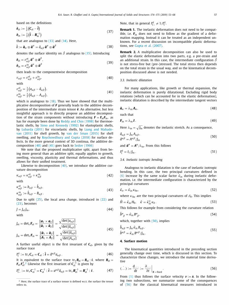
R.A. Sauer, R. Ghaffari and A. Gupta / International Journal of Solids and Structures 174–175 (2019) 53–68 55

Fig. 1. Surface description and kinematics: Multiplicative split into elastic and inelastic deformations and their relation to reference, intermediate and current configurations

S 0 , ˆ S and S .

H

c

F

t

g

a

w

n

T

a

g

r

a

g

d

a

[

a

l

a

b

T

[

t

κ

w

H

κ

r

a

s

d

d

a

F

m

f

o

f

ρ

t

o

t

3

fi

T

e

d

l

1

3

fi

d

t

d

u

n

ere ξα , for α = 1 , 2 , denotes the two curvilinear coordinates that

an be associated with a 2D parameter domain P as illustrated in

ig. 1 , while t ∈ [0, t end ] stands for time.

Given (1) , all geometrical aspects of the surface can be ob-

ained. The tangent plane at x ∈ S is characterized by the two tan-

ent vectors

α :=

∂ x

∂ ξα, (2)

hile the surface normal at x ∈ S is given by

=

a 1 × a 2

‖ a 1 × a 2 ‖

. (3)

he basis a 1 , a 2 and n allows to introduce the notion of in-plane

nd out-of-plane surface objects. The tangent vectors a 1 and a 2 are

enerally not orthonormal, meaning that the so-called surface met-

ic,

αβ := a α · a β, (4)

enerally gives [ a αβ ] � = [1 0 ; 0 1]. To restore orthonormality a set of

ual tangent vectors a

α is introduced from a α = a αβ a

β and a

α =

αβa β , 1 where [ a αβ ] := [ a αβ ] −1 , such that a

α · a β = δαβ

for [ δαβ

] =1 0 ; 0 1] . This illustrates a very important property of a αβ and

αβ : They lower or raise indices.

Another important surface characteristic is the curvature. It fol-

ows from the out-of-plane components of the second derivative

α, β := ∂ a α/ ∂ ξβ , denoted as

αβ := a α,β · n . (5)

hese components can be arranged in the matrix [ b αβ

] := a αγ b γβ ] , whose eigenvalues are the two principal surface curva-

ures

α = H ± √

H

2 − κ, (6)

here

:=

1 2

a αβ b αβ

:= det [ b αβ

] (7)

1 Following index notation, summation (from 1 to 2) is implied on all terms with

epeated Greek indices, i.e. a αβ a β = a α1 a 1 + a α2 a 2 .

t

F

re the mean curvature and Gaussian curvature of surface S, re-

pectively. The derivative a α, β is also referred to as the parametric

erivate of a α . It is generally different to the so-called co-variant

erivative of a α that is denoted by “;” and defined as

α;β := ( n � n ) a α,β . (8)

or general scalars and vectors (that have no free index) the para-

etric and co-variant derivates are identical. Only for objects with

ree indices (such as a α and a

α) a difference appears.

Analogous to (1) , physical fields on S are generally functions

f ξα and t. Examples are surface density ρ = ρ(ξα, t) and sur-

ace temperature T = T (ξα, t) . Their surface gradient follows from

,α (= ρ;α) and T ,α (= T ;α) as grad s ρ = ρ,α a

α and grad s T = T ,α a

α .

A more comprehensive treatment of the mathematical descrip-

ion of curved surfaces can be found in the classical textbooks

n differential geometry, e.g. see Kreyszig (1991) . A recent concise

reatment is also provided in Sauer (2018) .

. Surface kinematics

This section introduces reference, current and intermediate con-

guration, and discusses the kinematical quantities between them.

he discussion is restricted to Kirchhoff–Love kinematics. These are

ntirely based on the notion of surface strain and curvature, and

o not need any further kinematical measures. The description fol-

ows the classical treatment found in the works by Naghdi (1972,

982) , Pietraszkiewicz (1989) and Libai and Simmonds (1998) .

.1. Classical kinematical measures

Suppose that the surface S deforms over time. The initial con-

guration at time t = 0 is defined as reference configuration, and

enoted S 0 to distinguish it from the current configuration S at

ime t > 0. In order to distinguish all the surface quantities intro-

uced in Section 2 , upper case symbols (or the subscript "0") are

sed for the reference configuration, while lower case symbols (or

o subscript) are used for the current configuration, see Fig. 1 .

The primary measure relating S and S 0 is the surface deforma-

ion gradient

:= a α � A

α. (9)

56 R.A. Sauer, R. Ghaffari and A. Gupta / International Journal of Solids and Structures 174–175 (2019) 53–68

C

3

s

e

p

i

g

d

t

f

t

s

i

t

s

F

w

F

F

a

t

F

w

F

F

F

a

a

a

a

a

a

A

A

a

T

C

C

a

i

B

I

s

e

a

a

e

I

e

w

Together with its generalized inverse

F −1 = A α � a

α, (10)

it transforms the tangent vectors as

a α = F A α,

A α = F −1 a α,

A

α = F T a

α,

a

α = F −T A

α.

(11)

From F follow the two surface Cauchy–Green tensors

:= F T F = a αβ A

α� A

β,

B := F F T = A

αβ a α � a β . (12)

From these, the surface Green-Lagrange strain tensor

E :=

1 2

(C − I

)(13)

and the surface Almansi strain tensor

e :=

1 2

(i − B

−1 ), (14)

can be defined. Here,

I := A α � A

α = A αβ A

α� A

β,

i := a α � a

α = a αβ a

α� a

β(15)

denote the surface identity tensors on S 0 and S, respectively. E has

the components

E αβ := A α · E A β =

1 2

(a αβ − A αβ

), (16)

w.r.t. basis A

α , while e has the components

e αβ := a α · e a β =

1 2

(a αβ − A αβ

)(17)

w.r.t. basis a

α . To emphasize the equality e αβ = E αβ and, as is seen

later, the fact that the multiplicative split on F leads to an additive

split on these strain components, we introduce

ε αβ :=

1 2

(a αβ − A αβ

), (18)

such that

E = ε αβ A

α� A

β,

e = ε αβ a

α� a

β . (19)

Similar to (18) , we introduce the relative curvature components

καβ := b αβ − B αβ . (20)

The surface Cauchy–Green tensors have two invariants, I 1 and J . In

order to define them, the surface determinant of F is introduced

by

det s F :=

‖ F V 1 × F V 2 ‖

‖ V 1 × V 2 ‖

(21)

for all non-parallel surface tangent vectors V 1 and V 2 ( Javili et al.,

2014 ). Picking V α = A α, this leads to the second invariant

J := det s F =

‖ a 1 × a 2 ‖

‖ A 1 × A 2 ‖

, (22)

which is equal to

J =

√

det [ a αβ ] √

det [ A αβ ] , (23)

and corresponds to the local change of area between S 0 and S . The

first invariant is

αβ

I 1 = I : C = i : B = A a αβ . (24) e

.2. Kinematics of the multiplicative deformation split

The previous setting accounts only for a single deformation

ource. Its primary unknown is position x , from which everything

lse follows. In order to extend the setting to deformations com-

osed of two separate (i.e. elastic and inelastic) components, we

ntroduce the intermediate surface configuration

ˆ S with the tan-

ent vectors ˆ a α that are now an additional set of unknowns. The

eformation S 0 →

ˆ S is taken as the inelastic part, while ˆ S → S is

he elastic part, see Fig. 1 . Given the tangent vectors ˆ a α, the sur-

ace normal ˆ n , metric ˆ a αβ, inverse metric ˆ a αβ, dual tangent vec-

ors ˆ a

α, curvature components ˆ b αβ, mean curvature ˆ H and Gaus-

ian curvature ˆ κ are obtained analogous to expressions (3) –(7)

n Section 2 . The introduced intermediate configuration

ˆ S implies

hat the surface deformation gradient F can be multiplicatively

plit as

= F el F in , (25)

here

el := a α � ˆ a

α,

in :=

ˆ a α � A

α (26)

re the elastic and inelastic surface deformation gradients, respec-

ively. Split (25) implies the inverse split

−1 = F −1 in F −1

el , (27)

ith

−1 el :=

ˆ a α � a

α,

−1 in := A α � ˆ a

α.

(28)

el and F in transform the tangent vectors as

α = F el a α,

ˆ α = F −1

el a α,

ˆ

α = F T el a

α,

α = F −T el

ˆ a

α

(29)

nd

ˆ α = F in A α,

α = F −1 in ˆ a α,

α = F T in a

α,

ˆ

α = F −T in A

α.

(30)

hese relations can be used to push forward the right surface

auchy–Green tensor C to the intermediate configuration, i.e.

el := F −T in C F −1

in = F T el F el = a αβ ˆ a

α� ˆ a

β, (31)

nd to pull back the inverse left Cauchy–Green tensor B

−1 to the

ntermediate configuration, i.e.

−1 in := F T el B

−1 F el = F −T in F −1

in = A αβ ˆ a

α� ˆ a

β. (32)

n order to decompose the strain, it is convenient to introduce the

train tensor

ˆ := ε αβ ˆ a

α� ˆ a

β (33)

nalogous to (19) . This strain corresponds to the push forward of E

nd the pull-back of e to the intermediate configuration, since

ˆ = F −T

in E F −1 in = F T el e F el . (34)

nserting (13) or (14) into (34) gives

ˆ =

1 2

(C el − B

−1 in

)(35)

hich admits the simple additive decomposition

ˆ =

ˆ e el +

e in (36)

R.A. Sauer, R. Ghaffari and A. Gupta / International Journal of Solids and Structures 174–175 (2019) 53–68 57

b

e

e

t

i

d

e

e

t

ε

w

ε

ε

w

p

p

i

t

h

l

b

v

s

f

c

i

s

a

v

κ

w

κ

κ

D

(

J

w

J

J

A

s

I

I

F

I

r

N

R

i

m

k

t

R

s

a

i

o

p

3

i

r

i

a

s

F

H

a

a

a

I

3

b

(

m

p

κ

w

H

T

b

w

b

b

4

g

c

t

ased on the definitions

ˆ el :=

1 2

(C el − ˆ i

)ˆ in :=

1 2

(ˆ i − B

−1 in

) (37)

hat are analogous to (13) and (14) . Here,

:=

ˆ a α � ˆ a

α =

ˆ a αβ ˆ a

α� ˆ a

β (38)

enotes the surface identity on

ˆ S analogous to (15) . Introducing

ˆ el = ε el

αβˆ a

α� ˆ a

β,

ˆ in = ε in

αβˆ a

α� ˆ a

β(39)

hen leads to the componentwise decomposition

αβ = ε el αβ

+ ε in αβ

, (40)

ith

el αβ

=

1 2

(a αβ − ˆ a αβ

),

in αβ

=

1 2

(ˆ a αβ − A αβ

),

(41)

hich is analogous to (18) . Thus we have showed that the multi-

licative decomposition of F generally leads to the additive decom-

osition of the intermediate strain tensor ˆ e . An alternative, but less

nsightful approach is to directly propose an additive decomposi-

ion of the strain components without introducing F = F el F in , as

as for example been done by Reddy and Chin (1998) for thermoe-

astic shells, by Simo and Kennedy (1992) for elastoplastic shells,

y Lubarda (2011) for viscoelastic shells, by Liang and Mahade-

an (2011) for shell growth, by van der Sman (2015) for shell

welling, and by Roychowdhury and Gupta (2018) for surface de-

ects. In the more general context of 3D continua, the additive de-

omposition (40) and (41) goes back to Sedov (1966)

We note that the proposed multiplicative split, apart from be-

ng more general than an additive split, equally applies to growth,

welling, viscosity, plasticity and thermal deformations, and thus

llows for their unified treatment.

Likewise to decomposition (40) , we introduce the additive cur-

ature decomposition

αβ = κel αβ

+ κ in αβ (42)

ith

el αβ

:= b αβ − ˆ b αβ,

in αβ

:=

ˆ b αβ − B αβ . (43)

ue to split (25) , the local area change, introduced in (22) and

23) , becomes

= J el J in , (44)

ith

el = det s F el =

‖ a 1 × a 2 ‖

‖

a 1 × ˆ a 2 ‖

=

√

det [ a αβ ] √

det [ a αβ ] ,

in = det s F in =

‖

a 1 × ˆ a 2 ‖

‖ A 1 × A 2 ‖

=

√

det [ a αβ ] √

det [ A αβ ] .

(45)

further useful object is the first invariant of C el , given by the

urface trace

el 1 := tr s C el = C el : i =

ˆ a αβa αβ . (46)

t is equivalent to the surface trace tr s B el = B el : i , where B el = el F

T el .

2 Likewise the first invariant of C −1 el

is given by

el 1 − := tr s C

−1 el = C −1

el : i = a αβ ˆ a αβ = tr s B

−1 el = B

−1 el : i . (47)

2 Here, the surface trace of a surface tensor is defined w.r.t. the surface the tensor

efers to.

F

i

o

ote, that in general I el 1 − � = 1 /I el

1 .

emark 1. The inelastic deformation does not need to be compat-

ble, i.e. F in does not need to follow as the gradient of a defor-

ation mapping. Instead it can be treated as an independent un-

nown. For a recent discussion on incompatible plastic deforma-

ions, see Gupta et al. (2007) .

emark 2. A multiplicative decomposition can also be used to

plit the elastic deformation into two parts, e.g. a pre-strain and

n additional strain. In this case, the intermediate configuration S s not stress-free but (pre-)stressed. The total stress then depends

n the total strain in the usual way, and so the kinematical decom-

osition discussed above is not needed.

.3. Inelastic dilatation

For many applications, like growth or thermal expansion, the

nelastic deformation is purely dilatational. Excluding rigid body

otations (which can be accounted for in the elastic deformation),

nelastic dilatation is described by the intermediate tangent vectors

ˆ α = λin A α, (48)

uch that

in = λin I . (49)

ere λin =

√

J in denotes the inelastic stretch. As a consequence,

ˆ αβ = J in A αβ,

ˆ

αβ = A

αβ/J in (50)

nd

ˆ a

α = A

α/λin . From this follows

el 1 = I 1 /J in . (51)

.4. Inelastic isotropic bending

Analogous to inelastic dilatation is the case of inelastic isotropic

ending. In this case, the two principal curvatures defined in

6) increase by the same scalar factor κin during inelastic defor-

ation, i.e. the intermediate configuration is characterized by the

rincipal curvatures

ˆ α = κin κ0 α, (52)

here κ0 α are the two principal curvatures of S 0 . This implies

ˆ = κin H 0 , ˆ κ = κ2

in κ0 . (53)

his follows for example from considering the curvature relation

ˆ

αβ

= κin B

αβ, (54)

hich, together with (50) , implies

ˆ αβ = J in κin B αβ,

ˆ

αβ = κin B

αβ/J in . (55)

. Surface motion

The kinematical quantities introduced in the preceding section

enerally change over time, which is discussed in this section. To

haracterize these changes, we introduce the material time deriva-

ive

˙ ( . . . ) :=

d . . .

d t :=

∂ . . .

∂t

∣∣∣X = fixed

. (56)

rom (1) thus follows the surface velocity v :=

˙ x . In the follow-

ng two subsections, we summarize some of the consequences

f (56) for the classical kinematical measures introduced in

58 R.A. Sauer, R. Ghaffari and A. Gupta / International Journal of Solids and Structures 174–175 (2019) 53–68

a

κ

w

d

(

4

t

ε

ε

ε

w

a

A

d

I

f

F

C

A

g

a

A

i

a

Section 3.1 and the kinematical decomposition of Section 3.2 .

While the expressions in Section 4.1 appear in older works, those

of Section 4.2 are mostly new. They are required for formulat-

ing general constitutive models, as is discussed later ( Section 7 ).

Section 4.2 also exposes the coupling of elastic and inelastic con-

tributions that are present in some of the kinematical quantities.

4.1. Classical measures of the surface motion

From definition (18) follows the strain rate

˙ ε αβ =

1 2

˙ a αβ, (57)

where

˙ a αβ =

˙ a α · a β + a α · ˙ a β, (58)

according to (4) . With this we can find the material time derivative

of the area change J . Since J = J(a αβ ) = J(ε αβ ) , 3

˙ J =

∂ J

∂ a αβ˙ a αβ =

∂ J

∂ ε αβ˙ ε αβ (59)

From (23) and (57) follows

∂ J

∂ ε αβ= 2

∂ J

∂ a αβ= J a αβ, (60)

so that

˙ J

J =

1

2

a αβ ˙ a αβ . (61)

Similarly, the first invariant of C , I 1 = I 1 (a αβ ) = I 1 (ε αβ ) , gives

˙ I 1 =

∂ I 1 ∂ a αβ

˙ a αβ =

∂ I 1 ∂ ε αβ

˙ ε αβ, (62)

where

∂ I 1 ∂ ε αβ

= 2

∂ I 1 ∂ a αβ

= 2 A

αβ, (63)

due to (24) and (57) .

In order to express various curvature rates, we require

˙ n = −(a

α� n

)˙ a α, (64)

and

˙ a αβ =

∂ a αβ

∂ a γ δ˙ a γ δ, (65)

with

a αβγ δ :=

∂ a αβ

∂ a γ δ= −1

2

(a αγ a βδ + a αδa βγ

), (66)

see Sauer (2018) . From (20) then follows the relative curvature rate

˙ καβ =

˙ b αβ, (67)

with

˙ b αβ =

˙ a α,β · n + a α,β · ˙ n , (68)

due to (5) . Further, since H = H(a αβ, a αβ ) and κ = κ(a αβ, a αβ ) , we

find the mean curvature rate

˙ H =

∂H

∂ a αβ˙ a αβ +

∂H

∂ b αβ

˙ b αβ, (69)

with

∂H

∂ a αβ= −1

2

b αβ, ∂H

∂ b αβ=

1

2

a αβ, (70)

3 To simplify notation, the same symbol (here J ) is used for the variable and its

different functions. t

nd the Gaussian curvature rate

˙ =

∂κ

∂ a αβ˙ a αβ +

∂κ

∂ b αβ

˙ b αβ, (71)

ith

∂κ

∂ a αβ= −κ a αβ,

∂κ

∂ b αβ= 2 H a αβ − b αβ, (72)

ue to (7) and (65) ; see also Sauer (2018) . Relations (57) and

67) obviously imply

∂ . . .

∂ ε αβ= 2

∂ . . .

∂ a αβ,

∂ . . .

∂ καβ=

∂ . . .

∂ b αβ. (73)

.2. Decomposition of the surface motion

The additive strain decomposition of (40) and (41) directly leads

o the additive rate decomposition

˙ αβ = ˙ ε el αβ

+ ˙ ε in αβ

,

˙ el αβ

=

1 2

(˙ a αβ − ˙ ˆ a αβ

),

˙ in αβ

=

1 2

˙ ˆ a αβ,

(74)

here

˙ ˆ αβ =

˙ ˆ a α · ˆ a β +

a α · ˙ ˆ a β . (75)

lso the multiplicative decomposition of J leads to an additive rate

ecomposition: From (44) directly follows

˙ J

J =

˙ J el

J el

+

˙ J in J in

. (76)

n order to determine ˙ J el and

˙ J in , we first note that for a general

unction f (a αβ, a αβ ) = f (ε el αβ

, ε in αβ

) we have 4

˙ f =

∂ f

∂ a αβ˙ a αβ +

∂ f

∂ a αβ

˙ ˆ a αβ =

∂ f

∂ ε el αβ

˙ ε el αβ +

∂ f

∂ ε in αβ

˙ ε in αβ . (77)

rom (74) then follows

∂ f

∂ ε el αβ

= 2

∂ f

∂ a αβ,

∂ f

∂ ε in αβ

= 2

∂ f

∂ a αβ+ 2

∂ f

∂ a αβ

. (78)

ombing this with (73) leads to

∂ f

∂ ε el αβ

=

∂ f

∂ ε αβ. (79)

pplying (77) and (78) to f = J in ( a αβ ) = J in (ε in αβ

) defined in ( 45 .2)

ives

∂ J in ∂ ε el

αβ

= 0 , ∂ J in ∂ ε in

αβ

= J in ˆ a αβ(80)

nd

˙ J in J in

=

1

2

ˆ a αβ ˙ ˆ a αβ . (81)

pplying (77) and (78) to f = J el (a αβ, a αβ ) = J el (ε el αβ

, ε in αβ

) defined

n ( 45 .1) gives

∂ J el

∂ ε el αβ

= J el a αβ,

∂ J el

∂ ε in αβ

= J el

(a αβ − ˆ a αβ

)(82)

nd

˙ J el

J =

1

2

a αβ ˙ a αβ − 1

2

ˆ a αβ ˙ ˆ a αβ . (83)

el

4 Again the same symbol (here f ) is used for the variable and its different func-

ions.

R.A. Sauer, R. Ghaffari and A. Gupta / International Journal of Solids and Structures 174–175 (2019) 53–68 59

T

i

w

a

a

t

c

κ

κ

κ

w

b

a

n

a

w

F

t

w

A

b

a

fi

a

t

t

t

i

i

H

d

κ

d

5

e

t

w

M

o

w

r∫

w

m

a∫

5

t

a

t

c

m

5

w

t

i

ρ

w

i

i

i

i

he later equation agrees with (61), (76) and (81) .

Applying (78) to f = I el 1

= I el 1 (a αβ, a αβ ) = I el

1 (ε el

αβ, ε in

αβ) defined

n (46) gives

∂ I el 1

∂ ε el αβ

= 2

a αβ, ∂ I el

1

∂ ε in αβ

= 2

a αβγ δ(a γ δ − ˆ a γ δ

), (84)

here

ˆ

αβγ δ :=

∂ a αβ

∂ a γ δ

= −1

2

(ˆ a αγ ˆ a βδ +

ˆ a αδ ˆ a βγ), (85)

nalogous to (66) . ˙ I el 1

can then be obtained from (77) .

Next we turn towards the curvature rates. The additive curva-

ure decomposition in (42) and (43) leads to the additive rate de-

omposition

˙ αβ = ˙ κel αβ

+ ˙ κ in αβ

,

˙ el αβ

=

˙ b αβ − ˙ ˆ b αβ,

˙ in αβ

=

˙ ˆ b αβ,

(86)

here

˙ ˆ αβ =

˙ ˆ a α,β · ˆ n +

a α,β · ˙ ˆ n , (87)

nd

˙ ˆ = −

(ˆ a

α� ˆ n

)˙ ˆ a α, (88)

nalogous to (64) and (68) . In order to find various curvature rates,

e first note that for a general function f (a αβ, a αβ, b αβ, b αβ

)=

f (ε el αβ

, ε in αβ

, κel αβ

, κ in αβ

)we have

˙ f =

∂ f

∂ a αβ˙ a αβ +

∂ f

∂ a αβ

˙ ˆ a αβ +

∂ f

∂ b αβ

˙ b αβ +

∂ f

∂ b αβ

˙ ˆ b αβ,

=

∂ f

∂ ε el αβ

˙ ε el αβ +

∂ f

∂ ε in αβ

˙ ε in αβ +

∂ f

∂ κel αβ

˙ κel αβ +

∂ f

∂ κ in αβ

˙ κ in αβ . (89)

rom (74) and (86) then follow

∂ f

∂ κel αβ

=

∂ f

∂ b αβ,

∂ f

∂ κ in αβ

=

∂ f

∂ b αβ+

∂ f

∂ b αβ

(90)

ogether with the already known expressions in (78) . Combing this

ith (73) further leads to

∂ f

∂ κel αβ

=

∂ f

∂ καβ. (91)

pplying (78) and (90) to f =

ˆ H ( a αβ, b αβ ) =

ˆ H (ε in αβ

, κ in αβ

) defined

y ˆ H = ˆ a αβ ˆ b αβ/ 2 gives

∂ ˆ H

∂ ε el αβ

= 0 , ∂ ˆ H

∂ ε in αβ

= −ˆ b αβ, ∂ ˆ H

∂ κel αβ

= 0 , ∂ ˆ H

∂ κ in αβ

=

1

2

ˆ a αβ (92)

nalogous to (70) . ˙ ˆ H can then be obtained from (89) .

Applying (78) and (90) to f = ˆ κ( a αβ, b αβ ) = ˆ κ(ε in αβ

, κ in αβ

) de-

ned by ˆ κ = det [ b αβ ] / det [ a αβ ] gives

∂ κ

∂ ε el αβ

= 0 , ∂ κ

∂ ε in αβ

= −2 κ ˆ a αβ, ∂ κ

∂ κel αβ

= 0 ,

∂ κ

∂ κ in αβ

= 2

H

ˆ a αβ − ˆ b αβ, (93)

nalogous to (72) . ˙ ˆ κ can then be obtained from (89) . The fact that

he elastic derivatives in (92) and (93) are zero underlines the fact

hat the intermediate configuration is an independent unknown

hat is independent of ε el αβ

and κel αβ

.

On top of those expressions, the constitutive models discussed

n Section 7 require the dependency of H and κ on the elastic and

nelastic strain rates. Applying (78) and (90) to f = H(a αβ, b αβ ) =(ε el

αβ, ε in

αβ, κel

αβ, κ in

αβ) defined by (7) gives

∂H

∂ ε el αβ

=

∂H

∂ ε in αβ

= −b αβ, ∂H

∂ κel αβ

=

∂H

∂ κ in αβ

=

1

2

a αβ(94)

ue to (70) . Applying (78) and (90) to f = κ(a αβ, b αβ ) =(ε el

αβ, ε in

αβ, κel

αβ, κ in

αβ) defined by (7) gives

∂κ

∂ ε el αβ

=

∂κ

∂ ε in αβ

= −2 κ a αβ, ∂κ

∂ κel αβ

=

∂κ

∂ κ in αβ

= 2 H a αβ − b αβ,

(95)

ue to (72) .

. Surface balance laws

This section discusses the balance laws of mass, momentum,

nergy and entropy for curved surfaces. The derivation follows

he framework of Sauer and Duong (2017) and Sahu et al. (2017) ,

hich is based on the works by Prigogine (1961) , de Groot and

azur (1984) , Naghdi (1972) and Steigmann (1999) . It makes use

f three important theorems: Reynold’s transport theorem,

d

d t

∫ S

. . . d a =

∫ S

(˙ ( . . . ) +

˙ J

J ( . . . )

)d a, (96)

hich follows from substituting d a = J d A and using the product

ule, the surface divergence theorem,

∂S . . . να d s =

∫ S

. . . ;α d a, (97)

here να = a α · ν is the in-plane component of the boundary nor-

al ν and ”; α” is the co-variant derivative defined in Section 2 ,

nd the localization theorem

R

. . . d a = 0 ∀ R ⊂ S ⇔ . . . = 0 ∀ x ∈ S . (98)

.1. Surface mass balance

Mass balance is formulated here for the case of a mixture of

wo species. This could for example be a solvent diffusing into

matrix material and induce swelling. The partial surface densi-

ies ρ1 = ρ1 (ξα, t) and ρ2 = ρ2 (ξ

α, t) are introduced such that the

urrent surface density of the mixture is ρ = ρ1 + ρ2 (with unit

ass per current area).

.1.1. Total mass balance

Consider the Lagrangian description of the total mass balance

d

d t

∫ R

ρ d a =

∫ R

h d a ∀ R ⊂ S (99)

here h is a surface mass source (mass per current area and

ime) that originates for example from growth or swelling. Apply-

ng Reynolds’ transport theorem (96) and localization (98) gives

˙ + ρ ˙ J /J = h ∀ x ∈ S, (100)

hich is the governing ODE for ρ . In order to determine ρ( t ), the

nitial condition ρ = ρ0 at t = 0 is required.

If h = 0 , then ρ = ρ0 /J solves ODE (100) , which elegantly elim-

nates unknown ρ and its ODE.

If h � = 0, then ODE (100) needs to be solved (numerically). h � = 0

nduces growth, which is an inelastic deformation. An example is

sotropic growth discussed in Section 7.3.1 .

60 R.A. Sauer, R. Ghaffari and A. Gupta / International Journal of Solids and Structures 174–175 (2019) 53–68

s

m

S

w

K

s

σ

a

S

w

σ

a

S

w

b

μ

a

M

w

c

μ

a

μ

w

5

w

f

h

i

m

p

(

T

w

v

d

q

c

R

b

m

If b = b , as for gravity, we find b = b = b .

5.1.2. Partial mass balance

Additionally, the mass balance of the individual species needs

to be accounted for. Given (100) , it suffices to account for the mass

balance of one species. We therefore introduce the relative concen-

tration φ = ρ1 /ρ of species 1 and denote its source term h 1 . The

partial mass balance thus is

d

d t

∫ R

ρ φ d a =

∫ R

h 1 d a +

∫ ∂R

j ν d s ∀ R ⊂ S (101)

where the j ν term accounts for a relative mass flux of species

1 w.r.t. the average motion of the mixture. Defining the surface

mass flux vector j = j αa α through

j ν = − j · ν = − j α να (102)

and using the surface divergence theorem (97) on this term then

leads to ∫ R

(ρ ˙ φ + φ

(˙ ρ + ρ ˙ J /J

)− h 1 + j α;α

)d a = 0 ∀ R ⊂ S . (103)

Defining h ∗1

:= h 1 − φ h and making use of the localization theorem

(98) and ODE (100) , then gives

ρ ˙ φ = h

∗1 − j α;α ∀ x ∈ S (104)

which is the governing ODE for the relative concentration φ. In or-

der to determine φ( t ), the initial condition φ = φ0 at t = 0 is re-

quired. Interesting special cases for h ∗1

are h ∗1

= h 1 (the total mass

is conserved), h ∗1

= (1 − φ) h (only the mass of species 1 is in-

creasing), h ∗1 = −φ h (only the mass of species 2 is increasing) and

h ∗1

= 0 (the mass increase of species 1 and 2 has the ratio φ to

1 − φ).

5.2. Surface momentum balance

Before exploring momentum balance, the stress and bending

moments of the shell have to be introduced. As with the strains

discussed in Section 5.2.1 , these can be expressed w.r.t. the three

configurations S, S 0 and

ˆ S . Based on this, linear and angular mo-

mentum balance are then discussed in Sections 5.2.2 and 5.2.3 .

5.2.1. Stress and moment tensors

For shells, the Cauchy stress tensor takes the form

σ = N

αβ a α � a β + S α a α � n , (105)

with the in-plane membrane components N

αβ and the out-of-

plane shear components S α . The traction vector on the boundary

with normal ν = να a

α then follows from Cauchy’s formula

T = σT ν . (106)

Introducing

T α := σT a

α, (107)

then leads to T = T ανα .

For later reference the surface tension,

γ :=

1 2

tr s σ =

1 2 σ : 1 =

1 2

N

αβa αβ (108)

and the deviatoric surface stress,

σdev := σ − γ i (109)

are introduced. The latter has the in-plane components

N

αβdev

:= N

αβ − γ a αβ (110)

in basis a α . The out-of-plane component S α is identical for σdev

and σ .

The Cauchy stress describes the physical stress in configuration

S . It can be mapped to the (non-physical) second Piola-Kirchhoff

tress tensor S in configuration S 0 using the classical pull-back for-

ula

= J F −1

σ ˜ F −T

, (111)

here ˜ F := F + n � N is the full 3D deformation gradient for

irchhoff–Love kinematics. In the same fashion we introduce the

tress in configuration

ˆ S by

ˆ := J el ˜ F

−1

el σ ˜ F −T

el (112)

nd note that

= J in ˜ F −1

in ˆ σ ˜ F −T

in , (113)

here ˜ F el := F el + n � ˆ n and

˜ F in := F in +

n � N . This lead to

ˆ =

ˆ N

αβ ˆ a α � ˆ a β +

ˆ S α ˆ a α � ˆ n

(114)

nd

= N

αβ0

A α � A β + S α0 A α � N

(115)

here N

αβ0

:= J in ˆ N

αβ, ˆ N

αβ := J el N

αβ, S α0

:= J in ˆ S α and

ˆ S α := J el S α .

Similar to the stress tensor σ and the traction vector T , the

ending moment tensor

= −M

αβ a α � a β (116)

nd the moment vector

= μT ν = M

ανα, (117)

ith M

α = μT a

α, are introduced in configuration S . Just like σ, μan be pulled back to ˆ S and S 0 by

ˆ := J el ˜ F

−1

el μ ˜ F −T

el = − ˆ M

αβ ˆ a α � ˆ a β (118)

nd

0 := J ˜ F −1

μ ˜ F −T = −M

αβ0

A α � A β, (119)

here M

αβ0

:= J in ˆ M

αβ and

ˆ M

αβ := J el M

αβ .

.2.2. Linear surface momentum balance

The linear surface momentum balance is given by

d

d t

∫ R

ρ v d a =

∫ R

f d a +

∫ ∂R

T d s +

∫ R

h v d a ∀ R ⊂ S, (120)

here v :=

˙ x is the current surface velocity, f is a distributed sur-

ace load (force per current area) that, for two-species mixtures,

as contributions acting on species 1 and 2 (i.e. f = f 1 + f 2 ), T

s the traction vector on boundary ∂R and h v accounts for the

omentum change of the added mass. Applying Reynolds’ trans-

ort theorem (96) , surface divergence theorem (97) , localization

98) and ODE (100) gives

α;α + f = ρ ˙ v ∀ x ∈ S, (121)

hich is the governing PDE for the motion. In order to determine

( t ), the initial condition v = v 0 at t = 0 is required. In order to

etermine x ( t ), the additional initial condition x = X at t = 0 is re-

uired. PDE (121) is exactly the same as for the mass conserving

ase, e.g. see Sauer and Duong (2017) .

emark 3. The surface load can also be defined per mass, i.e.

:= f / ρ and then decomposed as f = ρb = ρ1 b 1 + ρ2 b 2 for the

ixture.

1 2 1 2

R.A. Sauer, R. Ghaffari and A. Gupta / International Journal of Solids and Structures 174–175 (2019) 53–68 61

5

w

l

σ

f

5

w

e

i

s

o

o

t

n

T

h

fl

q

t∫

U

∫,

s

P

ρ

w

i

f

s

w

ρ

a

R

c

f

w

D

a

G

σ

c

S

σ

R

f

q

p

o

(

5

w

p

a

t

n

t

η

D

q

t

t

ρ

w

i

u

s

H

(

T

I

w

b

c

t

i

.2.3. Angular surface momentum balance

Also the angular surface momentum balance

d

d t

∫ R

x × ρ v d a =

∫ R

x × f d a +

∫ ∂R

(x × T + m

)d s

+

∫ R

x × h v d a ∀ R ⊂ S, (122)

here m := n × M is a distributed moment acting on boundary ∂R ,

eads to the same local equations as before, i.e.

S α = −M

βα;β ,

αβ := N

αβ − b βγ M

γα is symmetric (123)

or all x ∈ S, e.g. see Sauer and Duong (2017) .

.3. Surface energy balance

The surface energy balance can be expressed as

d

d t

∫ R

ρ e d a =

∫ R

v · f d a +

∫ ∂R

(v · T +

˙ n · M

)d s +

∫ R

h e d a

+

∫ R

ρ r d a +

∫ ∂R

q ν d s ∀ R ⊂ S, (124)

here

= u +

1 2 v · v (125)

s the specific energy (per unit mass) at x ∈ B that contains the

tored energy u and the kinetic energy v · v /2. The first two terms

n the right hand side of (124) account for the mechanical power

f the external forces f and T and external moment M . The third

erm accounts for the power required to add mass h : power is

eeded to bring the added mass to energy level u and velocity v . 5

he last two terms account for the thermal power of an external

eat source r and a boundary influx q ν . Defining the surface heat

ux vector q = q αa α through

ν = −q · ν = −q ανα, (126)

he surface divergence theorem gives

∂R

q ν d s = −∫ R

q α;α d a . (127)

sing the surface divergence theorem on the v · T term gives

∂R

v · T d s =

∫ R

(v · T α;α +

1

2

σαβ ˙ a αβ + M

αβ ˙ b αβ

)d a −

∫ ∂R

˙ n · M d s

(128)

ee Sahu et al. (2017) . Using these two equations, ODE (100) and

DE (121) then gives

˙ u =

1 2 σαβ ˙ a αβ + M

αβ ˙ b αβ + ρ r − q α;α, ∀ x ∈ S, (129)

hich is the governing PDE for u . In order to determine u ( t ), the

nitial condition u = u 0 at t = 0 is required. PDE (129) has the same

ormat as in the classical case when h = 0 and no split of F is con-

idered ( Sahu et al., 2017 ). But due to the split of F , we can now

rite

˙ u = σαβ(

˙ ε el αβ + ˙ ε in αβ

)+ M

αβ(

˙ κel αβ + ˙ κ in

αβ

)+ ρ r − q α;α, ∀ x ∈ S,

(130)

ccording to Eqs. (57) , (67), (74) and (86) .

emark 4. The 1 2 σ

αβ ˙ a αβ d a term can also be rewritten as

1 2 σαβ ˙ a αβ d a = σ : D d a = S : ˙ E d A, (131)

5 If the added mass carries initial, nonzero energy e 0 , this energy contribution

an be accounted for in the ρ r term. Alternatively, if one does not wish to account

or e 0 in ρ r , h e in (124) should be replaced by h (e − e 0 ) .

T

t

here

=

1

2

˙ a αβ a

α� a

β,

˙ E =

1

2

˙ a αβ A

α� A

β, (132)

re the symmetric velocity gradient (e.g. see Sauer (2018) ) and the

reen-Lagrange strain rate (following from (13) ), respectively, and

and S are given by (105) and (111) . This illustrates that the stress

omponent σαβ (and energy 1 2 σ

αβ ˙ a αβ ) is expressed neither w.r.t.

0 nor S, but directly w.r.t. parameter space P ( Duong et al., 2017 ).

and S , on the other hand are specific to S and S 0 , respectively.

emark 5. In (124) the quantities e , f , T , M , r and q ν are defined

or the common mixture in order to avoid dealing with partial

uantities. In Sahu et al. (2017) , on the other hand, f is defined

artially, such that the second term in (124) is the area integral

ver v 1 · ρ1 b 1 + v 2 · ρ2 b 2 . This leads to an extra term in (129) and

130) if b 2 � = b 1 .

.4. Surface entropy balance

The surface entropy balance is given by

d

d t

∫ R

ρ s d a =

∫ R

(ρ ηe + ρ ηi + h s

)d a +

∫ ∂R

˜ q ν d s ∀ R ⊂ S,

(133)

here s is the specific entropy at x ∈ S, ηe is the external entropy

roduction rate caused by external loads and heat sources, ˜ q ν is

n entropy influx on the boundary of the surface, h s accounts for

he entropy increase due to the added mass, 6 and ηi is the inter-

al entropy production rate, which according to the second law of

hermodynamics satisfies

i ≥ 0 ∀ x ∈ S . (134)

efining the surface entropy flux vector ˜ q = ˜ q αa α through

˜ ν = −˜ q · ν = − ˜ q ανα (135)

he surface divergence theorem and the localization theorem lead

o the local equation

˙ s = ρ ηe + ρ ηi − ˜ q α;α ∀ x ∈ S, (136)

hich can be used to derive constitutive equations as is discussed

n Section 7 . For this, we introduce the Helmholtz free energy ψ := − T s, such that

˙ =

(˙ u − ˙ T s − ˙ ψ

)/T . (137)

ere T > 0 is the absolute temperature. Inserting this and PDE

130) into (136) then gives

ρ ˙ s = σαβ(

˙ ε el αβ + ˙ ε in αβ

)+ M

αβ(

˙ κel αβ + ˙ κ in

αβ

)+ ρ r − T

(q α

T

);α

− q αT ;αT

− ρ ˙ T s − ρ ˙ ψ . (138)

n deriving this equation we have used local energy balance (129) ,

hich in turn uses local mass balance (100) and local momentum

alance (121) . We have thus used all PDEs apart from the local

oncentration balance (104) . In order to account for it we add it to

he right hand side of (138) using the Lagrange multiplier method,

.e.

ρ ˙ s = . . . + μ(ρ ˙ φ − h

∗1 + j α;α

), (139)

6 If the added mass carries initial, nonzero entropy, this additional entropy con-

ribution can be accounted for in the ρ ηe term.

62 R.A. Sauer, R. Ghaffari and A. Gupta / International Journal of Solids and Structures 174–175 (2019) 53–68

i

v

s

g

t

t

a

b

t

t

R

e

a

t

t

fi

7

t

f

p

7

t

t

ψ

s

ψ

E

T

W

c

κ

7 Replacing ˙ ε el αβ

according to ( 74 .1), Eq. (148) can be also expressed in terms of

˙ ε αβ and ˙ ε in αβ

.

where μ is the Lagrange multiplier that corresponds to the chem-

ical potential as will be shown later. The last term in (139) can be

rewritten as

μ j α;α = T

(μ j α

T

);α

− T j α(μ

T

);α

(140)

in order to combine it with the T ( q α/ T ) ; α term. We thus find

T ρ ˙ s = ρ r − μ h

∗1 − T

(q α

T − μ j α

T

);α

+ σαβ(

˙ ε el αβ + ˙ ε in αβ

)

+ M

αβ(

˙ κel αβ + ˙ κ in

αβ

)− ρ s ˙ T − q αT ;α

T

+ ρ μ ˙ φ − T j α(μ

T

);α

− ρ ˙ ψ . (141)

On the right hand side here, the only source terms are the first two

terms, while the only divergence-like term is the third term. Com-

paring this with (136) , we can thus identify ηe = r/T − μ h ∗1 / (T ρ)

and ˜ q α = q α/T − μ j α/T , such that the second law (134) yields

T ρ ηi = σαβ(

˙ ε el αβ + ˙ ε in αβ

)+ M

αβ(

˙ κel αβ + ˙ κ in

αβ

)−ρ s ˙ T − q αT ;α

T + ρ μ ˙ φ − T j α

(μ

T

);α

− ρ ˙ ψ ≥ 0 . (142)

6. Problem statement

In this work we consider the case of coupling elastic deforma-

tions with either growth, swelling, viscosity, plasticity or thermal

deformation. So there is only coupling of two deformation types.

In principle three and more types can also be coupled. This would

require introducing further intermediate configurations. This sec-

tion discusses the strong form for the coupled two-field problem.

The recovery of the intermediate configuration is also addressed.

6.1. Strong form

The strong form can be unified by the problem statement: Find

x ( ξα , t ), ˆ a αβ (ξγ , t) and

ˆ b αβ (ξγ , t) satisfying PDE (121) and,

• for growth, ODE (100) . In this case, ˆ a αβ and

ˆ b αβ are either pre-

scribed or defined through ρ . So the primary unknowns are x

and ρ . Examples are given by Eqs. (50) , (55), (160) and (164) .

• for swelling, PDE (104) . In this case, ˆ a αβ and

ˆ b αβ are defined

through φ, e.g. by (50), (55), (165) and (166) , and so the pri-

mary unknowns are x and φ. If the swelling is not mass con-

serving (i.e. h � = 0), ρ is also unknown and needs to be obtained

from ODE (100) .

• for viscoelasticity and elastoplasticity, an evolution law (ODE)

for ˆ a αβ and

ˆ b αβ, like (185), (205), (214) or (223) .

• for thermoelasticity, PDE (130) . In this case, ˆ a αβ and

ˆ b αβ are

defined through T , e.g. by (50), (55), (227) and (228) , and so

the primary unknowns are x and T .

In general, the governing ODEs and PDEs are nonlinear and cou-

pled, and hence need to be solved numerically. The ODEs can be

solved locally using numerical integration schemes like the implicit

Euler scheme. The problem simplifies if ρ , φ or T are prescribed.

In those cases the problem decouples. In order to fully characterize

PDEs (104), (121) and (129) , constitutive expressions for the mass

flux, stress, bending moments and heat flux are needed. Those are

discussed in Section 7 .

6.2. Recovery of ˆ a α

Strictly the recovery of ˆ a 1 and

ˆ a 2 , which fully define the inter-

mediate configuration

ˆ S , is not needed to solve the problem, but

t may still be interesting to reconstruct ˆ a α, and from it F in , for

arious reasons.

The recovery is straightforward for isotropic growth, isotropic

welling and isotropic thermal expansion, since in these cases ˆ a α is

iven by (48) , with λin being either prescribed directly or defined

hrough ρ , φ or T , as in some of the examples of Section 7.3 .

For viscoelasticity and elastoplasticity, on the other hand, the

wo vectors ˆ a 1 and

ˆ a 2 can be determined from the two equations

ˆ αβ =

ˆ a α · ˆ a β

ˆ αβ =

ˆ a α,β · ˆ n

(143)

hat each have three cases. In order to eliminate rigid body rota-

ions, ˆ a 1 and

ˆ a 2 need to be fixed at some point.

emark 6. If no inelastic bending occurs, i.e. ˆ n = N , the second

quation can be replaced by the scalar equation

ˆ α · N = 0 , (144)

hat has two cases and fixes the inclination of ˆ S , and the condition

( a 1 × ˆ a 2 ) · N = ‖

a 1 × ˆ a 2 ‖ (145)

hat fixes the orientation of ˆ S . Additionally, ˆ a 1 (or ˆ a 2 ) needs to be

xed at a point to eliminate the rigid body rotation around N .

. Constitution

This section derives the constitutive equations following from

he second law of thermodynamics and provides various examples

or growth, swelling, elasticity, viscosity, plasticity and thermal ex-

ansion.

.1. Constitutive theory

In general, the Helmholtz free energy is supposed to be a func-

ion of the elastic strains ε el αβ

and κel αβ

, temperature T and concen-

ration φ, i.e.

= ψ

(ε el αβ

, κel αβ

, T , φ), (146)

uch that

˙ =

∂ψ

∂ ε el αβ

˙ ε el αβ +

∂ψ

∂ κel αβ

˙ κel αβ +

∂ψ

∂T ˙ T +

∂ψ

∂φ˙ φ . (147)

q. (142) then yields 7

ρ ηi =

(σαβ − ρ

∂ψ

∂ ε el αβ

)˙ ε el αβ + σαβ ˙ ε in αβ

+

(M

αβ − ρ∂ψ

∂ κel αβ

)˙ κel αβ + M

αβ ˙ κ in αβ

−ρ(

s +

∂ψ

∂T

)˙ T − T

q αT ;αT

+ ρ(μ − ∂ψ

∂φ

)˙ φ − T j α

(μ

T

);α

≥ 0 . (148)

e now invoke the procedure of Coleman and Noll (1964) . Two

ases have to be considered. The first case supposes that ε in αβ

and

in αβ

are independent process variables. Then, since (148) is true

R.A. Sauer, R. Ghaffari and A. Gupta / International Journal of Solids and Structures 174–175 (2019) 53–68 63

f

o

σ

M

s

μ

w

b

c

g

t

t

κ

I

S

fi

s

μ

t

c

t

A

t

m

7

o

e

�

t

w

o

c

�

D

e

d

w

�

w

�

i

i

c

σ

M

S

f

b

m

w

σ

M

7

e

s

t

c

ψ

A

e

t

7

b

s

(

J

w

a

b

g

or all rates ˙ ε el αβ

, ˙ ε in αβ

, ˙ κel αβ

, ˙ κ in αβ

˙ T , ˙ φ and gradients T ; α , ( μ/ T ) ; α , we

btain the sufficient conditions 8

αβ = ρ∂ψ

∂ ε el αβ

, σαβ ˙ ε in αβ

≥ 0 ,

αβ = ρ∂ψ

∂ κel αβ

, M

αβ ˙ κ in αβ

≥ 0 ,

= −∂ψ

∂T , q α T ;α ≤ 0 ,

=

∂ψ

∂φ, j α

(μ

T

);α

≤ 0 ,

(149)

hich are the general constitutive relations for the stresses σαβ ,

ending moments M

αβ , inelastic strains ε in αβ

, inelastic curvature

hange κ in αβ

, heat flux q α , entropy s , concentration flux j α and La-

range multiplier μ. The latter is identified to be the chemical po-

ential.

On the other hand, if ˙ ε in αβ

and ˙ κ in αβ

are functions of T and φ,

heir rates can be expanded into

˙ ε in αβ =

∂ ε in αβ

∂T ˙ T +

∂ ε in αβ

∂φ˙ φ,

˙ in αβ =

∂ κ in αβ

∂T ˙ T +

∂ κ in αβ

∂φ˙ φ . (150)

nserting this into (148) then yields

T ρ ηi =

(σαβ − ρ

∂ψ

∂ ε el αβ

)˙ ε el αβ +

(M

αβ − ρ∂ψ

∂ κel αβ

)˙ κel αβ

−ρ(

s +

∂ψ

∂T − σαβ

ρ

∂ ε in αβ

∂T − M

αβ

ρ

∂ κ in αβ

∂T

)˙ T − T

q αT ;αT

+ ρ(μ − ∂ψ

∂φ+

σαβ

ρ

∂ ε in αβ

∂φ+

M

αβ

ρ

∂ κ in αβ

∂φ

)˙ φ − T j α

(μ

T

);α

≥ 0 .

(151)

ince this is true for all ˙ ε el αβ

, ˙ κel αβ

, ˙ T , ˙ φ, T ; α and ( μ/ T ) ; α , we now

nd

= −∂ψ

∂T +

σαβ

ρ

∂ ε in αβ

∂T +

M

αβ

ρ

∂ κ in αβ

∂T ,

=

∂ψ

∂φ− σαβ

ρ

∂ ε in αβ

∂φ− M

αβ

ρ

∂ κ in αβ

∂φ,

(152)

ogether with the equations for σαβ and M

αβ and the inequality

onditions for q α and j α already listed in (149) . Now, the condi-

ions σαβ ˙ ε in αβ

≥ 0 and M

αβ ˙ κ in αβ

≥ 0 are no longer a requirement.

s (152) shows for the second case, the entropy and chemical po-

ential have contributions coming from the inelastic deformation

easures ε in αβ

and κ in αβ

.

.2. Alternative constitutive description

By redefining the Helmholtz free energy, we can rewrite some

f the above constitutive equations. Since the Helmholtz free en-

rgy ψ is defined per unit mass, the total energy is

:=

∫ ψ d m =

∫ ρ ψ d a (153)

M S

8 They are not necessary conditions as they can be combined into new condi-

ions.

J

here the first integral denotes the integration over the total mass

f surface S . Defining ρ0 as the current density in the reference

onfiguration, i.e. ρ0 := J ρ , we can also write

=

∫ S 0

ρ0 ψ d A . (154)

ue to growth ( h � = 0), density ρ0 is changing over time and is not

qual to the initial density ρ0 (unless h = 0 ). Likewise, we intro-

uce ˆ ρ as the density in

ˆ S , i.e. ˆ ρ := J el ρ, so that we can further

rite

=

∫ ˆ S

ˆ ρ ψ d

a =

∫ ˆ S

ˆ � d

a , (155)

here d a = J in d A and

ˆ := ˆ ρ ψ

(156)

s the Helmholtz free energy per unit intermediate area. Since ˆ ρ is

ndependent of the elastic deformation (as long as ˆ h = J el h is), 9 we

an rewrite the constitutive laws for σαβ and M

αβ into

αβ( el )

=

1

J el

∂ ˆ �

∂ ε el αβ

,

αβ( el )

=

1

J el

∂ ˆ �

∂ κel αβ

.

(157)

ubscript “(el)” is added here to indicate that this is the stress

ollowing from the elasticity model. But since σαβ( el )

= σαβ( in )

= σαβ,

rackets on this subscript are used. Using the alternative stress

easures introduced in (114) and using identities (79) and (91) ,

e can further write

ˆ αβ( el )

=

∂ ˆ �

∂ ε el αβ

=

∂ ˆ �

∂ ε αβ,

ˆ

αβ( el )

=

∂ ˆ �

∂ κel αβ

=

∂ ˆ �

∂ καβ.

(158)

.3. Constitutive examples

The following subsections give examples for the elastic and in-

lastic material behavior of curved surfaces resulting from the con-

titutive laws in (149), (152) and (157) . We therefore consider that

he Helmholtz free energy has additive mechanical, thermal and

oncentrational parts, i.e.

= ψ mech + ψ therm

+ ψ conc . (159)

n additional energy due to growth is not required since the en-

rgy change due to mass changes is already accounted for in �

hrough ρ , see (153) .

.3.1. Growth models

i. Isotropic in-plane growth: In this case ˆ a α and F in are given

y (48) and (49) . If this growth is unrestricted and maintains con-

tant density over time, i.e. J el = 1 and ρ = ρ0 = const. ∀ t , ODE

100) leads to the exponential growth law

in = J 0 exp (h t/ρ0 ) (160)

here J 0 is a dimensionless constant. In case of restricted growth

t changing density ( J el � = 1, ρ � = const.), expression (160) can still

e used as a possible model. However in that case, also other

rowth models in the form

in = J in (t) (161)

9 We can rewrite ODE (100) into ˙ ˆ ρ + ˆ ρ ˙ J in /J in − ˆ h = 0 .

64 R.A. Sauer, R. Ghaffari and A. Gupta / International Journal of Solids and Structures 174–175 (2019) 53–68

7

v

m

t

p

�

w

m

t

σ

a

p

a

�

w

a

f

σ

H

d

p

F

γ

a

σ

A

�

w

c

b

V

(

σ

w

σ

i

(

σ

w

c

11 A 3D energy density needs to be multiplied by the shell thickness in order to

are possible. Examples are linear 10 growth in h ,

J in = J 0 (1 + c h t

)2 (162)

and logarithmic expansion in time,

J in = J 0 (1 + ln (1 + t/t 0 )

)(163)

where J 0 , c and t 0 are constants. No matter what growth model is

used, if ρ is not assumed constant, it has to be solved for from ODE

(100) . If growth is mass conserving, e.g. during expansion (163) ,

ρ = ρ0 /J solves ODE (100) . Given J in , ˆ a αβ is then fully defined via

(50) .

ii. Curvature growth: An example for curvature growth is the

isotopic bending model (52) with the linear increase

κin = 1 + c h t (164)

that could be caused by a one-sided mass source h . ˆ b αβ is then

given by (55) .

7.3.2. Models for concentration induced swelling and diffusion

i. Linear isotropic swelling: A classical model for swelling is

the linear model

J in = λ2 in

, λin = 1 + αc (φ − φ0 ) (165)

where the material constant αc denotes the coefficient of chemical

swelling. Without loss of generality, one can then use ˆ a αβ = J in A αβ

as discussed in Section 3.3 .

ii. Chemical bending: An example for concentration induced

curvature increase is the isotopic bending model (52) with the lin-

ear curvature increase

κin = 1 + ακ (φ − φ0 ) (166)

where ακ is a constant. This curvature increase could be caused by

a one-sided swelling, e.g. due to the binding of molecules to one

side of a flexible membrane ( Sahu et al., 2017 ).

Another, less trivial, example is a curvature increase due to a

concentration difference between top and bottom surface, i.e.

κin = 1 + ακ

(φ+ − φ−

)(167)

where φ+ and φ− denote the top and bottom concentrations of

surface S, respectively. These need to be defined in a suitable way,

e.g. by using two separate PDEs of type (104) for the top and bot-

tom surface.

iii. Surface mass diffusion: A simple surface diffusion model

satisfying (149) is

j α = −M a αβ(μ

T

);β

(168)

where M is a constant. Choosing

ψ =

c φ

2

T φ2 (169)

where c φ is a constant, we find the chemical potential

μ = c φ T φ − 1

ρ J

(2 αc γ0 λin + 4 αc γ

M

0 λin κin + 2 ακ γ M

0 λ2 in

),

(170)

due to (152), (50), (55), (165) and (166) . Here γ0 := σαβ0

A αβ/ 2

and γ M

0 := M

αβ0

B αβ/ 2 follow from the stress definitions in

Eq. (123) and Section 5.2.1 . For the special case that γ 0 , γM

0 and

T are constant across S, we arrive at Fick’s law

j α = −D a αβ φ;β, (171)

where D = ˜ c φ M, with ˜ c φ = c φ −(2 α2

c γ0 + 4 α2 c γ

M

0 κin +

8 αc ακ γ M

0 λin

)/ (T ρ J) , is the surface diffusivity.

10 w.r.t. stretch λin =

√

J in

o

D

.3.3. Mechanical membrane models

This section discusses mechanical material models for elastic,

iscous and plastic membrane behavior, for which bending mo-

ents are neglected. In this case we have N

αβ = σαβ according

o (123) .

i. Surface elasticity: An example for the elastic response is the

otential

ˆ =

�

4

(J 2 el − 1 − 2 ln J el

)+

G

2

(I el 1 − 2 − 2 ln J el

), (172)

hich is adapted from the classical 3D Neo-Hookean material

odel ( Sauer and Duong, 2017 ). The parameters � and G are ma-

erial constants. From (172) follows the membrane stress

αβ( el )

=

�

2 J el

(J 2 el − 1

)a αβ +

G

J el

(ˆ a αβ − a αβ

), (173)

ccording to (157), (82) and (84) . The two terms in (172) do not

roperly split dilatational and deviatoric energies. Such a split is

chieved by the alternative model

ˆ =

K

4

(J 2 el − 1 − 2 ln J el

)+

G

2

(I el 1

J el

− 2

), (174)

hich is adapted from Sauer and Duong (2017) . The constants K

nd G denote the in-plane bulk and shear moduli. From (157) now

ollows the membrane stress

αβ( el )

=

K

2 J el

(J 2 el − 1

)a αβ +

G

J 2 el

(ˆ a αβ − I el

1

2

a αβ)

. (175)

ere the first part is purely dilatational, while the second is purely

eviatoric. Hence, the surface tension only depends on the first

art, while the deviatoric stress only depends on the second part:

rom (108) and (109) follow the surface tension

=

K

2 J el

(J 2 el − 1

)(176)

nd the deviatoric stress

αβdev

=

G

J 2 el

(ˆ a αβ − I el

1

2

a αβ)

. (177)

third elasticity example is the linear elastic membrane model

ˆ =

1

2

ε el αβ ˆ c αβγ δ ε el

γ δ, (178)

ith the material tangent

ˆ

αβγ δ := � ˆ a αβ ˆ a γ δ + G

(ˆ a αγ ˆ a βδ +

ˆ a αδ ˆ a βγ)

(179)

ased on the constants � and G . (178) is analogous to the 3D St.-

enant-Kirchhoff material, from which it can be derived. 11 From

158) now follows

ˆ αβ( el )

=

ˆ c αβγ δ ε el γ δ

, (180)

hich can be expanded into

ˆ αβ( el )

=

�

2

(I el 1 − 2

)ˆ a αβ + G

(ˆ a αγ a γ δ ˆ a βδ − ˆ a αβ

). (181)

i. Surface viscosity: A simple shear viscosity model satisfying

149) is

ˆ αβ( in )

= −η ˙ ˆ a αβ, (182)

here the material constant η ≥ 0 denotes the in-plane shear vis-

osity. 12 It is noted, that model (182) is not purely deviatoric, since

btain the membrane energy density ˆ � . 12 Proof: Using ˙ ˆ a αβ = − ˆ a αγ ˙ ˆ a γ δ ˆ a βδ and 2 D :=

˙ ˆ a αβ ˆ a α

� ˆ a β

gives σαβ( in )

ε in αβ

= 2 η ˆ D :

ˆ /J el ≥ 0 for η ≥ 0.

R.A. Sauer, R. Ghaffari and A. Gupta / International Journal of Solids and Structures 174–175 (2019) 53–68 65

Fig. 2. Surface rheology: a. viscoelastic Maxwell fluid; b. generalized viscoelastic solid; c. viscoelastic Kelvin solid. Even though these are 1D models, they can be used in 2D

and 3D, e.g. by applying them to dilatation and shear. E then plays the role of bulk and shear modulus.

i

A

σ

w

c

s

d

d

f

σ

w

c

(

a

w

i

t

a

t

J

f

(

M

t

σ

T

–

a

R

c

s

a

c

a

m

p

�

w

s

σ

i

k

i

�

w

e

σ

I

(

a

o

m

t

l

0

a

a

E

t

t

A

f

s

t

s

σ

T

ε

w

c

F

2

t generally leads to non-zero surface tension ( γ =

1 2 σ

αβ a αβ � = 0 ).

nother simple viscosity model satisfying (149) is

ˆ αβ( in )

= λ ˙ J in ˆ a αβ, (183)

here the material constant λ≥ 0 denotes the in-plane bulk vis-

osity. 13 It is noted, that model (183) is not purely dilatational,

ince it generally leads to non-zero shear stresses.

If there is no elastic deformation, ˆ a αβ = a αβ . If there is elastic

eformation, ˆ a αβ has to be determined from an evolution law. This

epends on the rheological model considered.

For a Maxwell element, see Fig. 2 a, the evolution law for ˆ a αβ

ollows from

αβ( el )

(ˆ a γ δ

)= σαβ

( in )

(ˆ a γ δ, ˙ ˆ a γ δ

), (184)

hich is a nonlinear ODE that can be solved locally using numeri-

al methods (e.g. implicit Euler). For example, for models (173) and

182) , the evolution law is

˙ ˆ

αβ =

�

2 η

(1 − J 2 el

)a αβ +

G

η

(a αβ − ˆ a αβ

), (185)

here J el is a function of ˆ a αβ according to (45) . A second example

s to use models (175) and (183) and consider only inelastic dilata-

ion ( a αβ = J in A αβ ) according to Section 3.3 . Contracting (184) with

αβ and using the relations from Section 3.3 thus yields the evolu-

ion law

˙ in =

K

λ

J

I 1

(J

J in − J in

J

)(186)

or J in .

For a generalized viscoelastic solid, see Fig. 2 b, evolution law

184) needs to be solved for ˆ a αβM

within each Maxwell element

. This defines the stress σαβM

in each Maxwell element. The to-

al stress is then the sum of the stresses in all elements, i.e.

αβ = σαβel 0

(a γ δ

)+

∑

M=1

σαβM

(ˆ a γ δM

). (187)

his model contains the special cases of a single Maxwell element

for M = 1 and σαβel 0

= 0 – and the Kelvin model – for M = 1 and

ˆ αβ = a αβ (see Fig. 2 c).

emark 7. Apart of (182) and (183) , also the slightly different

hoices σαβ( in )

= −η ˙ ˆ a αβ and σαβ( in )

= λ ˙ J in ˆ a αβ are consistent with the

econd law.

iii. Surface constraints: Constraints are important for various

pplications. A popular example is incompressibility, which is dis-

ussed in the following.

Elastic incompressibility implies J el ≡ 1. This conditions leads to

n extra stress that can for example be captured by the Lagrange

ultiplier method. According to this, the stress follows from the

otential

ˆ = q (J el − 1

), (188)

13 Proof: From (81) follows σαβ( in )

ε in αβ

= 2 λ ˙ J 2 in

/J ≥ 0 for λ≥ 0.

w

i

here q is the corresponding Lagrange multiplier. The constraint

tress, according to (157) and (82) , thus is

αβ( el )

= q a αβ, (189)

.e. it is dilatational. The Lagrange multiplier q is an additional un-

nown that needs to be solved for. It can be avoided by consider-

ng the penalty regularization

ˆ =

K

2

(J el − 1

)2 , (190)

here the in-plane bulk modulus K is set to a very large value to

nsure J el ≈ 1. From (157) and (82) now follows

αβ( el )

= K

(J el − 1

)a αβ . (191)

nelastic incompressibility implies J in ≡ 1, i.e. ˙ J in = 0 . According to

81) this leads to the constraint

˙ ˆ

αβ ˆ a αβ = 0

(192)

n the internal variable ˆ a αβ . This is a scalar equation, and so two

ore equations are needed in order to determine ˆ a αβ . We can find

hose by contracting the evolution law with ˆ a αβ and a αβ . For evo-

ution law (185) we thus find

= �(1 − J 2

el

)+ G

(2 − 4 /I el

1 −)

(193)

nd

˙ ˆ

αβa αβ =

�

η

(1 − J 2 el

)+

G

η

(2 − I el

1

). (194)

qs. (192) –(194) can then be solved for ˆ a αβ .

iv. Surface plasticity: Plastic behavior can be characterized by

he yield surface f y = f y (σαβ ) = 0 that satisfies ˙ f y = 0 during plas-

ic flow. Hence,

∂ f y ∂ σαβ

˙ σαβ = 0 . (195)

common approach to determine an evolution equation for ˆ a αβ

rom this is to use the principle of maximum dissipation. This as-

umes that for a given inelastic strain rate ˙ ε in αβ

, the true stress is

he one that maximizes the dissipation σαβ ˙ ε in αβ

among all possible

tress states. This implies

˙ αβ ˙ ε in αβ

= 0 . (196)

ogether, Eqs. (195) and (196) imply that

˙ in αβ

= λ∂ f y

∂ σαβ, (197)

hich is the evolution law for ˆ a αβ . The scalar λ follows from the

ondition

˙ f y = 0 .

An example (that is a 2D version of von Mises plasticity 14 , see

ig. 3 a) is

f y :=

ˆ s −√

2

σy , (198)

14 Another possibility is to use the classical 3D von Mises plasticity model together

ith the plane stress assumption. In this case f y := ‖ σdev ‖ −√

2 / 3 σy , where ˜ σdev

s the full 3D stress deviator. See Fig. 3 b.

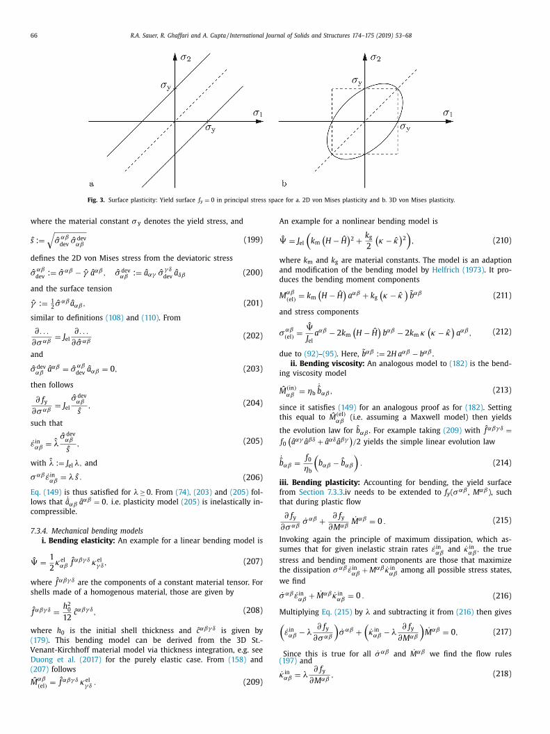
66 R.A. Sauer, R. Ghaffari and A. Gupta / International Journal of Solids and Structures 174–175 (2019) 53–68

Fig. 3. Surface plasticity: Yield surface f y = 0 in principal stress space for a. 2D von Mises plasticity and b. 3D von Mises plasticity.

V

A

�

w

a

d

M

a

σ

d

i

M

s

t

t

b

i

f

t

I

s

s

t

w

σ

M (

(

κ

where the material constant σ y denotes the yield stress, and

ˆ s :=

√

ˆ σαβdev

ˆ σ dev αβ

(199)

defines the 2D von Mises stress from the deviatoric stress

ˆ σαβdev

:= ˆ σαβ − ˆ γ ˆ a αβ, ˆ σ dev αβ

:=

ˆ a αγ ˆ σγ δdev

ˆ a δβ (200)

and the surface tension

ˆ γ :=

1 2

ˆ σαβ ˆ a αβ, (201)

similar to definitions (108) and (110) . From

∂ . . .

∂ σαβ= J el

∂ . . .

∂ σαβ(202)

and

ˆ σ dev αβ

ˆ a αβ = ˆ σαβdev

ˆ a αβ = 0 , (203)

then follows

∂ f y ∂ σαβ

= J el

ˆ σ dev αβ

ˆ s , (204)

such that

˙ ε in αβ

=

ˆ λˆ σ dev αβ

ˆ s , (205)

with

ˆ λ := J el λ, and

σαβ ˙ ε in αβ

= λ ˆ s . (206)

Eq. (149) is thus satisfied for λ≥ 0. From (74), (203) and (205) fol-

lows that ˙ ˆ a αβ ˆ a αβ = 0 , i.e. plasticity model (205) is inelastically in-

compressible.

7.3.4. Mechanical bending models

i. Bending elasticity: An example for a linear bending model is

ˆ � =

1

2

κel αβ

ˆ f αβγ δ κel γ δ,

(207)

where ˆ f αβγ δ are the components of a constant material tensor. For

shells made of a homogenous material, those are given by

ˆ f αβγ δ =

h

2 0

12

ˆ c αβγ δ, (208)

where h 0 is the initial shell thickness and ˆ c αβγ δ is given by

(179) . This bending model can be derived from the 3D St.-

enant-Kirchhoff material model via thickness integration, e.g. see

Duong et al. (2017) for the purely elastic case. From (158) and

(207) follows

ˆ M

αβ( el )

=

ˆ f αβγ δ κel γ δ

. (209)

n example for a nonlinear bending model is

ˆ = J el

(k m

(H − ˆ H

)2 +

k g

2

(κ − ˆ κ

)2 ), (210)

here k m

and k g are material constants. The model is an adaption

nd modification of the bending model by Helfrich (1973) . It pro-

uces the bending moment components

αβ( el )

= k m

(H − ˆ H

)a αβ + k g

(κ − ˆ κ

)˜ b αβ (211)

nd stress components

αβ( el )

=

ˆ �

J el

a αβ − 2 k m

(H − ˆ H

)b αβ − 2 k m

κ(κ − ˆ κ

)a αβ, (212)

ue to (92) –(95) . Here, ˜ b αβ := 2 H a αβ − b αβ .

ii. Bending viscosity: An analogous model to (182) is the bend-

ng viscosity model

ˆ

( in ) αβ

= ηb ˙ ˆ b αβ, (213)

ince it satisfies (149) for an analogous proof as for (182) . Setting

his equal to ˆ M

( el ) αβ

(i.e. assuming a Maxwell model) then yields

he evolution law for ˆ b αβ . For example taking (209) with

ˆ f αβγ δ =f 0

(ˆ a αγ ˆ a βδ + ˆ a αδ ˆ a βγ

)/ 2 yields the simple linear evolution law

˙ ˆ αβ =

f 0 ηb

(b αβ − ˆ b αβ

). (214)

ii. Bending plasticity: Accounting for bending, the yield surface

rom Section 7.3.3 .iv needs to be extended to f y ( σαβ , M

αβ ), such

hat during plastic flow

∂ f y ∂ σαβ

˙ σαβ +

∂ f y ∂ M

αβ˙ M

αβ = 0 . (215)

nvoking again the principle of maximum dissipation, which as-

umes that for given inelastic strain rates ˙ ε in αβ

and ˙ κ in αβ

, the true

tress and bending moment components are those that maximize

he dissipation σαβ ˙ ε in αβ

+ M

αβ ˙ κ in αβ

among all possible stress states,

e find

˙ αβ ˙ ε in αβ

+

˙ M

αβ ˙ κ in αβ

= 0 . (216)

ultiplying Eq. (215) by λ and subtracting it from (216) then gives

˙ ε in αβ − λ∂ f y

∂ σαβ

)˙ σαβ +

(˙ κ in αβ − λ

∂ f y ∂ M

αβ

)˙ M

αβ = 0 , (217)

Since this is true for all ˙ σαβ and

˙ M

αβ we find the flow rules197) and

˙ in αβ = λ∂ f y

∂ M

αβ, (218)

R.A. Sauer, R. Ghaffari and A. Gupta / International Journal of Solids and Structures 174–175 (2019) 53–68 67

w

f

w

i

s

w

M

a

γ

i

r

a

κ

w

t

S

(

e

K

b

7

�

w

p

s

d

T

(

T

m

q

w

(

i

J

w

m

J

t

b

v

c

κ

a

i

o

κ

w

f

e

t

t

b

8

e

p

r

t

e

e

a

i

s

e

r

a

a

c

p

a

t

a

e

p

m

i

fi

S

A

(

t

m

R

A

A

A

B

B

B

C

D

hich are the evolution laws for ˆ a αβ and

ˆ b αβ . The scalar λ again

ollows from the condition

˙ f y = 0 .

As an example we consider the simple extension of (198) ,

f y :=

ˆ s

σy +

ˆ s M

M y −

√

2

2

, (219)

here the material constant M y denotes the yield limit for bend-

ng, and

ˆ M

:=

√

ˆ M

αβdev

ˆ M

dev αβ

(220)

ith

ˆ

αβdev

:=

ˆ M

αβ − ˆ γM

ˆ a αβ, ˆ M

dev αβ

:=

ˆ a αγ ˆ M

γ δdev

ˆ a δβ (221)

nd

ˆ M

:=

1 2

ˆ M

αβ ˆ a αβ, (222)

s defined analogous to (199) –(201) . Due to this analogy, the flow

ule for κ in αβ

follows in analogy to (205) , which is still valid here,

s

˙ in αβ

=

ˆ λˆ M

dev αβ

ˆ s M

, (223)

hich also satisfies Eq. (149) for λ≥ 0.

The elasto-plasticity model described by the constitutive equa-

ions in (157), (197) and (218) is equivalent to the model of

imo and Kennedy (1992) . However, in Simo and Kennedy (1992) ,

157) is written in terms of � = ρ0 ψ, the Helmholtz free en-

rgy per unit reference area (in the case of h = 0 ). Also, Simo and

ennedy (1992) , consider an alternative model to (219) that is

ased on Shapiro (1961) .

.3.5. Thermal models

i. Thermal energy: Considering

ˆ = C H

[ (T − T 0 ) − T ln

T

T 0

] , (224)

here C H is a material constant and T 0 is a constant reference tem-

erature ( Holzapfel, 20 0 0 ), gives the specific entropy

=

C H ˆ ρ

ln

T

T 0 , (225)

ue to (149) and (156) . This energy does not generate stresses.

hose only appear in response to mechanical deformations. Due to

224) , the stored energy (per intermediate area) is ˆ ρ u = ˆ ρ (ψ + s ) = C H (T − T 0 ) .

ii. Surface heat conduction: A simple surface conductivity

odel satisfying (149) is Fourier’s law

α = −k a αβ T ;β (226)

here the constant k is the surface heat conductivity. Model

226) is analogous to Fick’s law (171) .

iii. Thermal surface expansion: A simple linear model for

sotropic thermal expansion (analogous to chemical swelling) is

in = λ2 in

, λin = 1 + αT (T − T 0 ) , (227)

here the material constant αT denotes the coefficient of ther-

al expansion. Without loss of generality, one can then use ˆ a αβ = in A αβ as discussed in Section 3.3 . Model (227) leads to an addi-

ional entropy contribution due to (152) , analogous to the contri-

ution in μ seen in (170) .

iv. Thermal bending: An example for temperature induced cur-

ature increase is the isotopic bending model (52) with the linear

urvature increase

¯ in = 1 + ακ (T − T 0 ) (228)

nalogous to (166) . Here ακ is a material constant. This curvature

ncrease could be caused by a one-sided thermal expansion. Anal-

gous to (167) , one can also consider the model

¯ in = 1 + ακ

(T + − T −

)(229)

here T + and T − denote the top and bottom temperatures of sur-

ace S, respectively. Those need to be defined in a suitable way,

.g. by using two separate PDEs of type (129) for the top and bot-

om surface. Note that, models (228) and (229) lead to an addi-

ional entropy contribution due to (152) , analogous to the contri-

ution in μ seen in (170) .

. Conclusion

This work presents a general nonlinear shell theory for coupled

lastic and inelastic deformations, accounting for growth, swelling,

lasticity, viscosity and thermal expansion. The formulation is de-

ived from the balance laws of mass, momentum, energy and en-

ropy using a multiplicative split of the surface deformation gradi-

nt into elastic and inelastic contributions. The general constitutive

quations of this coupling are derived and illustrated by several ex-

mples. Those generally require the derivatives of various kinemat-

cal quantities w.r.t. the elastic and inelastic deformations.

Although the present formulation is purely theoretical, it is

uitable for computational analysis, for example within the finite

lement method. There has been important recent progress on

otation-free finite elements (FE) in the framework of isogeometric

nalysis ( Kiendl et al., 2009 ). Such FE formulations allow for a very

ccurate yet efficient surface description that is particularly benefi-

ial for an accurate representation of curvatures. It can thus be ex-

ected that isogeometric shell FE formulations for coupled inelastic

nd elastic deformations would be very beneficial. So far, it seems

hat only elasto-plasticity and isotropic thermoelasticity have been

nalyzed with multiplicatively split isogeometric shell FE ( Ambati

t al., 2018; Vu-Bac et al., 2019 ). But the authors are currently ap-

lying the present theory to extend the hyperelastic graphene FE

odel of Ghaffari and Sauer (2018) to anisotropic thermoelastic-

ty ( Ghaffari and Sauer, 2019 ), and to study the growth of fluid

lms using the FE model of Sauer (2014) and Roohbakhshan and

auer (2019) .

cknowlgedgments

The authors are grateful to the German Research Foundation

DFG ) for funding this research under grant GSC 111 . The au-

hors also like to thank Farshad Roohbakhshan for feedback on the

anuscript.

eferences

hmad, S. , Irons, B.M. , Zienkiewicz, O.C. , 1970. Analysis of thick and thin shell struc-tures by curved finite elements. Int. J. Numer. Meth. Eng. 2 (3), 419–451 .

ltenbach, H. , Eremeyev, V. , 2015. On the constitutive equations of viscoelastic mi-cropolar plates and shells of differential type. Math. Mech. Complex Syst. 3 (3),

273–283 . mbati, M. , Kiendl, J. , De Lorenzis, L. , 2018. Isogeometric Kirchhoff–Love shell for-

mulation for elasto-plasticity. Comput. Methods Appl. Mech. Eng. 340, 320–339 .

a s ar, Y. , Weichert, D. , 1991. A finite-rotation theory for elastic-plastic shells underconsideration of shear deformations. ZAMM 71 (10), 379–389 .

etsch, P. , Stein, E. , 1999. Numerical implementation of multiplicative elasto-plas-ticity into assumed strain elements with application to shells at large strains.

Comput. Methods Appl. Mech. Eng. 179 (3), 215–245 . ilby, B.A. , Lardner, L.R.T. , Stroh, A.N. , 1957. Continuous distributions of dislocations

and the theory of plasticity. In: Actes du IXe Congrès International de Mé-canique Appliquée (Bruxelles, 1956), volume 8. Université libre de Bruxelles,

pp. 35–44 .

oleman, B.D. , Noll, W. , 1964. The thermodynamics of elastic materials with heatconduction and viscosity. Arch. Ration. Mech. Anal. 13, 167–178 .

ervaux, J. , Ciarletta, P. , Amar, M.B. , 2009. Morphogenesis of thin hyperelasticplates: a constitutive theory of biological growth in the Föppl-von Kármán limit.

J. Mech. Phys. Solids 57 (3), 458–471 .

68 R.A. Sauer, R. Ghaffari and A. Gupta / International Journal of Solids and Structures 174–175 (2019) 53–68

P

R

R

R

S

S

S

S

S

S

S

S

S

v

S

S

V

V

V

V

W

Dörr, D. , Schirmaier, F.J. , Henning, F. , Kärger, L. , 2017. A viscoelastic approach formodeling bending behavior in finite element forming simulation of continu-

ously fiber reinforced composites. Compos. Part A 94, 113–123 . Dujc, J. , Brank, B. , 2012. Stress resultant plasticity for shells revisited. Comput. Meth-

ods Appl. Mech. Engrg. 247–248, 146–165 . Duong, T.X. , Roohbakhshan, F. , Sauer, R.A. , 2017. A new rotation-free isogeomet-

ric thin shell formulation and a corresponding continuity constraint for patchboundaries. Comput. Methods Appl. Mech. Eng. 316, 43–83 .

Eberlein, R. , Wriggers, P. , 1999. Finite element concepts for finite elastoplastic strains

and isotropic stress response in shells: theoretical and computational analysis.Comput. Methods Appl. Mech. Eng. 171 (3), 243–279 .

Eckart, C. , 1948. The thermodynamics of irreversible processes. IV. The theory ofelasticity and anelasticity. Phys. Rev. 73, 373–382 .

Flory, P.J. , 1950. Statistical mechanics of swelling of network structures. J. Chem.Phys. 18 (1), 108–111 .

Ghaffari, R. , Duong, T.X. , Sauer, R.A. , 2017. A new shell formulation for graphene

structures based on existing ab-initio data. Int. J. Solids Struct. 135, 37–60 . Ghaffari, R. , Sauer, R.A. , 2018. A new efficient hyperelastic finite element model for

graphene and its application to carbon nanotubes and nanocones. Finite Ele.Anal. Des. 146, 42–61 .

Ghaffari, R., Sauer, R. A., 2019. Nonlinear thermomechanical formulations foranisotropic volume and surface continua. arXiv: 1901.00917 .

Green, A.E. , Naghdi, P.M. , 1979. On thermal effects in the theory of shells. Proc. R.

Soc. A 365 (1721), 161–190 . Green, A.E. , Naghdi, P.M. , Osborn, R. , 1968. Theory of an elastic-plastic cosserat sur-

face. Int. J. Solids Struct. 4 (9), 907–927 . de Groot, S.R. , Mazur, P. , 1984. Non-Equilibrium Thermodynamics. Dover .

Gupta, A. , Steigmann, D.J. , Stölken, J. , 2007. On the evolution of plasticity and in-compatibility. Math. Mech. Solids 12, 583–610 .

Helfrich, W. , 1973. Elastic properties of lipid bilayers: theory and possible experi-

ments. Z. Naturforsch. 28c, 693–703 . Holzapfel, G.A. , 20 0 0. Nonlinear Solid Mechanics: A Continuum Approach for Engi-

neering. Wiley, Hoboken . Javili, A. , Mc Bride, A. , Steinmann, P. , Reddy, B.D. , 2014. A unified computational

framework for bulk and surface elasticity theory: a curvilinear-coordinate-basedfinite element methodology. Comput. Mech. 54 (3), 745–762 .

Kar, V.R. , Panda, S.K. , 2016. Nonlinear thermomechanical deformation behaviour of

P-FGM shallow spherical shell panel. Chin. J. Aeronaut. 29 (1), 173–183 . Kiendl, J. , Bletzinger, K.U. , Linhard, J. , Wüchner, R. , 2009. Isogeometric shell anal-

ysis with Kirchhoff–Love elements. Comput. Methods Appl. Mech. Eng. 198,3902–3914 .

Kondaurov, V.I. , Nikitin, L.V. , 1987. Finite strains of viscoelastic muscle tissue. J. Appl.Math. Mech. 51 (3), 346–353 .

Kondo, K. , 1949. A proposal of a new theory concerning the yielding of materials

based on Riemannian geometry, i. J. Soc. Appl. Mech. Jpn. 2 (11), 123–128 . Kreyszig, E. , 1991. Differential geometry. Dover .

Kröner, E. , 1959. Allgemeine kontinuumstheorie der versetzungen und eigenspan-nungen. Arch. Ration. Mech. Anal. 4 (1), 273 .

Li, F. , 2012. A justification of two-dimensional nonlinear viscoelastic shells model.Abstr. Appl. Anal. 2012, 24 .

Liang, H. , Mahadevan, L. , 2011. Growth, geometry, and mechanics of a blooming lily.Proc. Natl. Acad. Sci. 108 (14), 5516–5521 .

Libai, A. , Simmonds, J.G. , 1998. The Nonlinear Theory of Elastic Shells, second ed.

Cambridge University Press, Cambridge . Lubarda, V.A. , 2004. Constitutive theories based on the multiplicative decomposi-

tion of deformation gradient: thermoelasticity, elastoplasticity, and biomechan-ics. Appl. Mech. Rev. 57 (2), 95–108 .

Lubarda, V.A. , 2011. Rate-type elasticity and viscoelasticity of an erythrocyte mem-brane. J. Mech. Mater. Struct. 6 (1), 361–376 .

Lucantonio, A. , Tomassetti, G. , De Simone, A. , 2017. Large-strain poroelastic plate

theory for polymer gels with applications to swelling-induced morphing ofcomposite plates. Compos. Part B 115, 330–340 .

Lychev, S. , 2014. Equilibrium equations for transversely accreted shells. ZAMM 94(1–2), 118–129 .

Miehe, C. , 1998. A theoretical and computational model for isotropic elastoplasticstress analysis in shells at large strains. Comput. Methods Appl. Mech. Eng. 155

(3), 193–233 .

Naghdi, P.M. , 1972. Theory of plates and shells. In: Truesdell, C. (Ed.), Handbuch derPhysik. Springer, Berlin, pp. 425–640 .

Naghdi, P.M. , 1982. Finite deformation of elastic rods and shells. In: Carlson, D.E.,Shields, R.T. (Eds.), Proceedings of the IUTAM Symposium on Finite Elasticity.

The Hague. Martinus Nijhoff Publishers, pp. 47–103 . Neff, P. , 2005. A geometrically exact viscoplastic membrane-shell with viscoelastic

transverse shear resistance avoiding degeneracy in the thin-shell limit. ZAMP

56 (1), 148–182 . Papastavrou, A. , Steinmann, P. , Kuhl, E. , 2013. On the mechanics of continua

with boundary energies and growing surfaces. J. Mech. Phys. Solids 61 (6),1446–1463 .

arisch, H. , 1978. Geometrical nonlinear analysis of shells. Comput. Methods Appl.Mech. Eng. 14 (2), 159–178 .

Pietraszkiewicz, W. , 1989. Geometrically nonlinear theories of thin elastic shells.Adv. Mech. 12 (1), 51–130 .

Prigogine, I. , 1961. Introduction to Thermodynamics of Irreversible Processes. Inter-science Publishers .

Rausch, M.K. , Kuhl, E. , 2014. On the mechanics of growing thin biological mem-branes. J. Mech. Phys. Solids 63, 128–140 .

Reddy, J.N. , Chin, C.D. , 1998. Thermomechanical analysis of functionally graded

cylinders and plates. J. Therm. Stresses 21 (6), 593–626 . Reina, C. , Djodom, L.F. , Ortiz, M. , Conti, S. , 2018. Kinematics of elasto-plasticity: va-

lidity and limits of applicability of F = F e F p for general three-dimensional de-formations. J. Mech. Phys. Solids 121, 99–113 .

oohbakhshan, F. , Sauer, R.A. , 2016. Isogeometric nonlinear shell elements for thinlaminated composites based on analytical thickness integration. J. Micromech.

Mol. Phys. 1 (3–4), 1640010 .

Roohbakhshan, F. , Sauer, R.A. , 2017. Efficient isogeometric thin shell formulations forsoft biological materials. Biomech. Model. Mechanobiol. 16 (5), 1569–1597 .

oohbakhshan, F. , Sauer, R.A. , 2019. A finite membrane element formulation for sur-factants. Colloids Surf. A 566, 84–103 .

oychowdhury, A. , Gupta, A. , 2018. On structured surfaces with defects: geometry,strain incompatibility, stress field, and natural shapes. J. Elast. 131, 239–276 .

ahu, A. , Sauer, R.A. , Mandadapu, K.K. , 2017. Irreversible thermodynamics of curved

lipid membranes. Phys. Rev. E 96, 042409 . Sauer, R.A. , 2014. Stabilized finite element formulations for liquid membranes and

their application to droplet contact. Int. J. Numer. Methods Fluids 75 (7),519–545 .

auer, R.A. , 2018. On the computational modeling of lipid bilayers using thin-shelltheory. In: Steigmann, D. (Ed.), CISM Advanced School ‘On the role of mechanics

in the study of lipid bilayers’. Springer, pp. 221–286 .

auer, R.A. , Duong, T.X. , 2017. On the theoretical foundations of solid and liquidshells. Math. Mech. Solids 22 (3), 343–371 .

auer, R.A. , Duong, T.X. , Mandadapu, K.K. , Steigmann, D.J. , 2017. A stabilized finite el-ement formulation for liquid shells and its application to lipid bilayers. J. Com-

put. Phys. 330, 436–466 . awczuk, A. , 1982. On plastic shell theories at large strains and displacements. Int.

J. Mech. Sci. 24 (4), 231–244 .

edov, L. , 1966. Foundations of the Non-Linear Mechanics of Continua. PergamonPress, Oxford .

hapiro, G.S. , 1961. On yield surfaces for ideally plastic shells. In: Problems of Con-tinuum Mechanics. SIAM, Philadelphia, pp. 414–418 .

idoroff, F. , 1974. Un modèle viscoélastique non linéaire avec configuration intermé-diaire. J. Méc. 13 (4), 679–713 .

imo, J.C. , Kennedy, J.G. , 1992. On a stress resultant geometrically exact shell model.

part v. nonlinear plasticity: formulation and integration algorithms. Comput.Methods Appl. Mech. Eng. 96, 133–171 .

an der Sman, R.G.M. , 2015. Hyperelastic models for hydration of cellular tissue.Soft Matter 11, 7579–7591 .

Steigmann, D.J. , 1999. On the relationship between the Cosserat and Kirchhoff–Lovetheories of elastic shells. Math. Mech. Solids 4, 275–288 .

Steigmann, D.J. , 2015. Mechanics of materially uniform thin films. Math. Mech.Solids 20 (3), 309–326 .

tojanovi c, R. , Djuri c, S. , Vujoševi c, L. , 1964. On finite thermal deformations. Archi-

wum Mechaniki Stosowanej 1 (16), 103108 . Stumpf, H. , Schieck, B. , 1994. Theory and analysis of shells undergoing finite elas-

tic-plastic strains and rotations. Acta Mech. 106 (1), 1–21 . wain, D. , Gupta, A. , 2018. Biological growth in bodies with incoherent interfaces.

Proc. R. Soc. A 474, 20170716 . Takamizawa, K. , Hayashi, K. , 1987. Strain energy density function and uniform strain

hypothesis for arterial mechanics. J. Biomech. 20 (1), 7–17 .

etter, R. , Stoop, N. , Jenni, T. , Wittel, F.K. , Herrmann, H.J. , 2013. Subdivision shellelements with anisotropic growth. Int. J. Numer. Methods Eng. 95 (9), 791–

810 . etter, R. , Stoop, N. , Wittel, F.K. , Herrmann, H.J. , 2014. Simulating thin sheets: buck-

ling, wrinkling, folding and growth. J. Phys. 487 (1), 012012 . u-Bac, N. , Duong, T.X. , Lahmer, T. , Areias, P. , Sauer, R.A. , Park, H.S. , Rabczuk, T. ,

2019. A NURBS-based inverse analysis of thermal expansion induced morphing

of thin shells. Comput. Methods Appl. Mech. Eng. 350, 480–510 . u-Bac, N. , Duong, T.X. , Lahmer, T. , Zhuang, X. , Sauer, R.A. , Park, H.S. , Rabczuk, T. ,

2018. A NURBS-based inverse analysis for reconstruction of nonlinear defor-mations in thin shell structures. Comput. Methods Appl. Mech. Eng. 331, 427–

455 . ang, J. , Steigmann, D.J. , Wang, F.F. , Dai, H.H. , 2018. On a consistent finite-strain

plate theory of growth. J. Mech. Phys. Solids 111, 184–214 .

Zimmermann, C. , Toshniwal, D. , Landis, C.M. , Hughes, T.J.R. , Mandadapu, K.K. ,Sauer, R.A. , 2019. An isogeometric finite element formulation for phase

fields on deforming surfaces. Comput. Methods Appl. Mech. Eng. 351, 441–477 .