international journal on advances in networks and services
TRANSCRIPT


The International Journal on Advances in Networks and Services is published by IARIA.
ISSN: 1942-2644
journals site: http://www.iariajournals.org
contact: [email protected]
Responsibility for the contents rests upon the authors and not upon IARIA, nor on IARIA volunteers,
staff, or contractors.
IARIA is the owner of the publication and of editorial aspects. IARIA reserves the right to update the
content for quality improvements.
Abstracting is permitted with credit to the source. Libraries are permitted to photocopy or print,
providing the reference is mentioned and that the resulting material is made available at no cost.
Reference should mention:
International Journal on Advances in Networks and Services, issn 1942-2644
vol. 2, no. 4, year 2009, http://www.iariajournals.org/networks_and_services/
The copyright for each included paper belongs to the authors. Republishing of same material, by authors
or persons or organizations, is not allowed. Reprint rights can be granted by IARIA or by the authors, and
must include proper reference.
Reference to an article in the journal is as follows:
<Author list>, “<Article title>”
International Journal on Advances in Networks and Services, issn 1942-2644
vol. 2, no. 4, year 2009,<start page>:<end page> , http://www.iariajournals.org/networks_and_services/
IARIA journals are made available for free, proving the appropriate references are made when their
content is used.
Sponsored by IARIA
www.iaria.org
Copyright © 2009 IARIA

Internet and Web Services
Thomas Michael Bohnert, SAP Research, Switzerland
Serge Chaumette, LaBRI, University Bordeaux 1, France
Dickson K.W. Chiu, Dickson Computer Systems, Hong Kong
Matthias Ehmann, University of Bayreuth, Germany
Christian Emig, University of Karlsruhe, Germany
Geoffrey Fox, Indiana University, USA
Mario Freire, University of Beira Interior, Portugal
Thomas Y Kwok, IBM T.J. Watson Research Center, USA
Zoubir Mammeri, IRIT – Toulouse, France
Bertrand Mathieu, Orange-ftgroup, France
Mihhail Matskin, NTNU, Norway
Guadalupe Ortiz Bellot, University of Extremadura Spain
Dumitru Roman, STI, Austria
Monika Solanki, Imperial College London, UK
Vladimir Stantchev, Berlin Institute of Technology, Germany
Pierre F. Tiako, Langston University, USA
Weiliang Zhao, Macquarie University, Australia
Wireless and Mobile Communications
Habib M. Ammari, Hofstra University - Hempstead, USA
Thomas Michael Bohnert, SAP Research, Switzerland
David Boyle, University of Limerick, Ireland
Xiang Gui, Massey University-Palmerston North, New Zealand
Qilian Liang, University of Texas at Arlington, USA
Yves Louet, SUPELEC, France
David Lozano, Telefonica Investigacion y Desarrollo (R&D), Spain
D. Manivannan (Mani), University of Kentucky - Lexington, USA
Jyrki Penttinen, Nokia Siemens Networks - Madrid, Spain / Helsinki University of Technology,
Finland
Radu Stoleru, Texas A&M University, USA
Jose Villalon, University of Castilla La Mancha, Spain
Natalija Vlajic, York University, Canada
Xinbing Wang, Shanghai Jiaotong University, China
Qishi Wu, University of Memphis, USA
Ossama Younis, Telcordia Technologies, USA
Sensors
Saied Abedi, Fujitsu Laboratories of Europe LTD. (FLE)-Middlesex, UK
Habib M. Ammari, Hofstra University, USA
Steven Corroy, University of Aachen, Germany
Zhen Liu, Nokia Research – Palo Alto, USA

Winston KG Seah, Institute for Infocomm Research (Member of A*STAR), Singapore
Peter Soreanu, Braude College of Engineering - Karmiel, Israel
Masashi Sugano, Osaka Prefecture University, Japan
Athanasios Vasilakos, University of Western Macedonia, Greece
You-Chiun Wang, National Chiao-Tung University, Taiwan
Hongyi Wu, University of Louisiana at Lafayette, USA
Dongfang Yang, National Research Council Canada – London, Canada
Underwater Technologies
Miguel Ardid Ramirez, Polytechnic University of Valencia, Spain
Fernando Boronat, Integrated Management Coastal Research Institute, Spain
Mari Carmen Domingo, Technical University of Catalonia - Barcelona, Spain
Jens Martin Hovem, Norwegian University of Science and Technology, Norway
Energy Optimization
Huei-Wen Ferng, National Taiwan University of Science and Technology - Taipei, Taiwan
Qilian Liang, University of Texas at Arlington, USA
Weifa Liang, Australian National University-Canberra, Australia
Min Song, Old Dominion University, USA
Mesh Networks
Habib M. Ammari, Hofstra University, USA
Stefano Avallone, University of Napoli, Italy
Mathilde Benveniste, Wireless Systems Research/En-aerion, USA
Andreas J Kassler, Karlstad University, Sweden
Ilker Korkmaz, Izmir University of Economics, Turkey
Centric Technologies
Kong Cheng, Telcordia Research, USA
Vitaly Klyuev, University of Aizu, Japan
Arun Kumar, IBM, India
Juong-Sik Lee, Nokia Research Center, USA
Josef Noll, ConnectedLife@UNIK / UiO- Kjeller, Norway
Willy Picard, The Poznan University of Economics, Poland
Roman Y. Shtykh, Waseda University, Japan
Weilian Su, Naval Postgraduate School - Monterey, USA
Multimedia
Laszlo Boszormenyi, Klagenfurt University, Austria
Dumitru Dan Burdescu, University of Craiova, Romania
Noel Crespi, Institut TELECOM SudParis-Evry, France
Mislav Grgic, University of Zagreb, Croatia

Hermann Hellwagner, Klagenfurt University, Austria
Polychronis Koutsakis, McMaster University, Canada
Atsushi Koike, KDDI R&D Labs, Japan
Chung-Sheng Li, IBM Thomas J. Watson Research Center, USA
Parag S. Mogre, Technische Universitat Darmstadt, Germany
Eric Pardede, La Trobe University, Australia
Justin Zhan, Carnegie Mellon University, USA
Additional reviews by:
Jorjeta Jetcheva, Carnegie Mellon, USA

International Journal on Advances in Networks and Services
Volume 2, Number 4, 2009
CONTENTS
MAC Protocols for Wireless Sensor Networks: Tackling the Problem of Unidirectional
Links
Stephan Mank, Brandenburg University of Technology, Germany
Reinhardt Karnapke, Brandenburg University of Technology, Germany
Jörg Nolte, Brandenburg University of Technology, Germany
218 - 229
A Novel Fault Diagnosis Technique in Wireless Sensor Networks
Anas Abu Taleb, University of Bristol, UK
J. Mathew, University of Bristol, UK
D.K. Pradhan, University of Bristol, UK
Taskin Kocak, Bahcesehir University, Turkey
230 - 240
Integrated System for Malicious Node Discovery and Self-destruction in Wireless Sensor
Networks
Madalin Plastoi, Politehnica University of Timisoara, Romania
Ovidiu Banias, Politehnica University of Timisoara, Romania
Daniel-Ioan Curiac, Politehnica University of Timisoara, Romania
Constantin Volosencu, Politehnica University of Timisoara, Romania
Roxana Tudoroiu, Politehnica University of Timisoara, Romania
Alexa Doboli, State University of New York, Stony Broke, USA
241 - 250
A Novel Approach to Indoor Location Systems Using Propagation Models in WSNs
Gomes Gonçalo, Instituto Superior Técnico Inesc-ID, Portugal
Sarmento Helena, Instituto Superior Técnico Inesc-ID, Portugal
251 - 260
New Sensing Model for Wireless Sensor Networks
Peter Soreanu, ORT Braude College, Israel
Zeev (Vladimir) Volkovich, ORT Braude College, Israel
261 - 272
FastM: Design and Evaluation of a Fast Mobility Mechanism for Wireless Mesh Networks
Luís Couto, Universidade de Aveiro, Portugal
João Paulo Barraca, Universidade de Aveiro, Portugal
Susana Sargento, Universidade de Aveiro, Portugal
Rui L. Aguiar, Universidade de Aveiro, Portugal
273 - 286

MAC Protocols for Wireless Sensor Networks:Tackling the Problem of Unidirectional Links
Stephan Mank, Reinhardt Karnapke, Jorg NolteDistributed Systems/Operating Systems Group
Brandenburg University of TechnologyCottbus, Germany
{smank, karnapke, jon}@informatik.tu-cottbus.de
Abstract—Experiments have shown that unidirectional linksare quite common in wireless sensor networks. Still, manyMAC protocols ignore their existence, even though they havea tremendous impact on the performance of both TDMA- andcontention based protocols. In contention based protocols themedium may be assumed free when it is indeed busy. In TDMAbased protocols two neighboring nodes might get assigned thesame slot even though there is an unidirectional link betweenthem. In this paper we discuss the influence of unidirectionallinks on communication protocols in wireless sensor networks,focusing on MAC protocols. We also present two protocols thatdo not only eliminate the negative side effects of unidirectionallinks, but use them for message transmission as well.
Keywords-Wireless Sensor Networks; MAC Protocols; Uni-directional Links
I. INTRODUCTION
Wireless sensor networks are collections of small sensingand computation units that can cooperate with each otherusing over the air communication. Since these networksshall be deployed on a large scale (i.e. hundreds of nodes),the overall cost often dictates the usage of cheap radiotransceivers. Many of these transceivers do not only lackhardware support for medium access control, their hugenumber also makes it near to impossible to calibrate allof them exactly the same, resulting in many differencesin antennae characteristics. Due to these differences, whichare also enhanced by the difference in orientation of thedeployed nodes, a lot of unidirectional links (node A cansend to node B but not vice versa) are introduced intothe sensor network right from the beginning. Differencesin height of position are also an influencing factor. After thesensor network is started, dynamic effects like atmosphericchanges, animals walking by or people using electricaldevices lead to an often changing radio neighborhood.These changes can be a complete breakage of links, or thetransformation from a unidirectional to a bidirectional oneand vice versa. Sometimes a unidirectional link changes itsdirection.
Most of todays sensor networks are meant to deliverthe gathered data in one form or another to a sink forevaluation. But this requires multihop transmissions alongchanging routes. Finding a suitable route is the task of
routing protocols, the MAC protocol only needs to supplyone hop communication. Unidirectional links are a com-mon phenomenon on both protocol layers - most routingprotocols try to eliminate the negative effect they have ontheir routing choices, only some of them try to utilize them.MAC protocols face a harder problem, as the effect of aunidirectional link may not only be a wrong choice, buta lot of collisions leading to a bad channel utilization andpacket loss.
In this paper we present the influences of unidirectionallinks on both protocol layers, and describe a way of increas-ing network connectivity, reliability and lifetime by using theunidirectional links in addition to the bidirectional ones inMLMAC-UL (TDMA-based) and ECTS-MAC (contentionbased), both presented first at Sensorcomm 2009 [1]. Theeffectiveness for both different approaches is shown insimulations as well as in experiments with TMote Sky sensornodes.
This paper is structured as follows: Section II takesa closer look at unidirectional links, their occurrence inwireless sensor networks and their impact on routing andMAC protocols. Section III describes related work, whilesections IV and V describe the protocols MLMAC-UL andECTS-MAC respectively. In section VI our two protocolsare evaluated, both with simulations and experiments onreal sensor network hardware. We finish with conclusionand future work in section VII.
II. THE NATURE OF UNIDIRECTIONAL LINKS
In theory a unidirectional link is defined quite simple. Alink from node A to node B is unidirectional, if Node B canreceive messages from A, but not vise versa. In practice, itis fairly hard to establish such criteria. It is not possible tomonitor the status of all links globally. You can only measurethe status of a link at a certain time. Moreover, only onedirection of the link can be measured because transceiverscan not transmit and receive at the same time. Worse still,links change over time. Due to e.g. atmospheric changesor someone walking into the area, a link that seems to bebidirectional at one moment can become unidirectional atany time.
218
International Journal on Advances in Networks and Services, vol 2 no 4, year 2009, http://www.iariajournals.org/networks_and_services/
The authors of [2] describe an experiment they conductedin the Luneburger Heide. The original aim was to evaluatea routing protocol, which is not characterized further in thepaper. Rather, the observations they made concerning theproperties of the wireless medium are described, focusingon the frequency of changes and the poor stability of links.These experiments were conducted using 24 Scatterweb ESB[3] sensor nodes, which were affixed to trees, poles etc,and left alone for two weeks after program start. One ofthe duties of the network was the documentation of thelogical topology (radio neighborhood of nodes), which wasevaluated by building a new routing tree every hour, e.g.for use in a sense-and-send application. The neighborhoodwas evaluated using the Wireless Neighborhood Explorationprotocol (WNX) [2], which can detect unidirectional andbidirectional links. Once this was done, all unidirectionallinks were discarded and only the bidirectional ones wereused to build the routing tree. Figure 1a shows one complete
Figure 1. A Communication Graph from [2] (Presentation) [4]
communication graph obtained by WNX, while figure 1bshows the same graph without unidirectional links, where alot of redundant paths have been lost by the elimination. Infact, one quarter of the nodes are only connected to the restof the network by a single link when unidirectional linksare removed. If this single link breaks, the nodes becomeseparated, even though there are still routes available. Thus,the removal of unidirectional links increases the probabilityof network separation severely.
The authors of [5] hold a similar view. They evaluatethe three kinds of links (asymmetric, unidirectional, bidi-rectional) using protocols like ETX (Expected TransmissionCount) [6]. These protocols search for reliable links, butmost focus on bidirectional ones. This leads to the factthat a link with a reliability of 50% in both directions ischosen above one with 100% from node A to node B and0% from B to A. If data needs to be transmitted only fromA to B without need for acknowledgment, this choice isobviously wrong. To prevent this wrong choice, the authors
of [5] propose a protocol called ETF (Expected Numberof Transmissions over Forward Links), which is able touse unidirectional links. They also show that the reach ofreliable unidirectional links is greater that that of reliablebidirectional links. In experiments with XSM motes [5] 7times 7 nodes were placed in a square, with a distance ofabout 1 meter between nodes. In four sets of experiments atdifferent times of day each node sent 100 messages at threedifferent power levels. Then the packet reception rate wasrecorded, which is defined for a node A as the number ofpackets A received from a node B divided by the numberof messages sent (100). Then the packet reception rates ofnodes A and B are compared. If the difference is less than10%, the link is considered bidirectional. If it is more then90% the link is considered unidirectional. The XSM nodesoffer 9 different transmission strengths, of which three wereevaluated: the lowest, the highest and the third in between.Table I shows the results of the experiments.
Table ILINK QUALITY VERSUS TRANSMISSION STRENGTH
PRR less than 10% 10-90% more than 90% linkspower level 1 50% 43% 7% 500power level 3 65% 22% 13% 1038power level 9 88% 6% 6% 1135
The results show that even when using the maximumtransmission strength 12% of the links would have beendiscarded by ETX (Expected Transmission Count) [6] andsimilar link quality evaluation protocols that focus onlyon bidirectional links. As the lifetime is one of the ma-jor optimization goals in a sensor network and receiv-ing/transmitting consumes a lot of energy, it is rather uncom-mon to have all nodes constantly transmit using the highesttransmission strength. In fact, current research projects likee.g. [7] try to minimize power consumption by adjusting thetransmission strength depending on the required reach andreliability.
The observations of [5] are concluded in three points:1) Wireless links are often asymmetric, especially if
transmission power is low2) Dense networks produce more asymmetric links then
sparse ones3) Symmetric links only bridge short distances, while
asymmetric and especially unidirectional ones have amuch longer reach. A conclusion drawn from this factis that the usage of unidirectional links in a routingprotocol can increase the efficiency of a routing pro-tocol considering energy and/or latency.
A sensor network which monitors water pumps withinwells is described in [8]. The sensors were used to monitorthe water level, the amount of water taken and the saltinessof the water in a number of wells which were widely
219
International Journal on Advances in Networks and Services, vol 2 no 4, year 2009, http://www.iariajournals.org/networks_and_services/

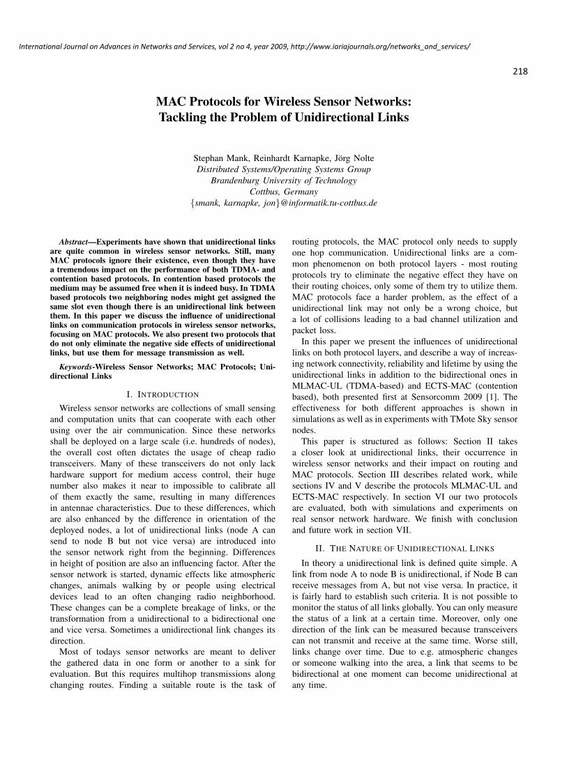
distributed. The necessity for this sensor network arosebecause the pumps were close to shore and a rise in saltinesswas endangering the quality of the water. The averagedistance between wells was 850 meters and the range oftransmission was about 1500 meters. Communication wasrealized using 802.11 WLAN hardware both for the nodesas well as for the gateway. For data transmission betweennodes Surge Reliable [9] was used, which makes routingdecisions based on the link quality between nodes.
Figure 2. A Communication Graph from [8] that Follows the Theory
During the experiments the authors observed, that the(logical) topology of the network changed dynamically,even though all nodes were stationary. The authors claimthat these changes were probably due to antenna size andchanges in temperature and air moisture. In this context itis important to remember that the distance of nodes was farbelow the range of the transmitters (about 50%). While about70% of the routing trees observed followed the theory (figure2), there were a lot of strange exceptions. In one case theaverage distance between connected nodes even rose to 1135meters, as nodes that should have been able to communicatedirectly with the gateway were connected to nodes on the farside instead. In one of these routing trees (figure 3), a singlenode had to take care of all communication with the gateway,even nodes that were on the other side were using it asnext hop. The reason for this is that Surge Reliable choosesthe nodes with the best link quality, but only considersbidirectional links. If unidirectional links could have beenused, the results could have been quite different.
VigilNet, a military sensor network for terrain surveillanceis described in [10]. This project aims at the detection ofmoving vehicles using magnetic sensors attached to Mica2sensor nodes. The transport of messages from the nodesto the sink was realized using a diffusion based algorithm,similar to Directed Diffusion [11], which produced a routing
Figure 3. A Communication Graph from [8] with Long and Strange Links
tree with root at the sink. To eliminate unidirectional links,a protocol called Link Symmetry Detection was developed.Each node periodically transmitted the list of its neighbors.A node that received such a neighbor list checked the list todetermine if it was mentioned. If it was not, the link was anincoming unidirectional one. When building the routing treeafter deployment, the transmission power of all nodes washalved. Now all nodes determined their parent node fromthe neighbor lists received with this half strength. At the endof this setup phase, all nodes switched to full transmissionpower. The intention behind this scheme was to ensure thatthe connection to the father node would not break. Duringthe experiments, the authors noted that asymmetric linkswere far more common than expected. They put this factdown to differences in hardware, as the transceivers were notcalibrated before the experiment. Another interesting effectseen in these experiments is that only about 2/3 of all nodeswere able to communicate directly with the sink, becauseonly bidirectional links were used.
III. RELATED WORK
The problem of unidirectional links has been recognizedbefore, and protocols have been developed which can usethem.
The Multicast MAC protocol (MMP) [12] does not di-rectly address the problem of unidirectional links, but itoffers an easy way to realize a multicast communication,which can easily be increased to broadcast. BMMM [13] andMaclayer Multicast [14] follow a similar approach. MMPis an extension of the IEEE 802.11 MAC in DCF mode.The Request To Send (RTS) message of MMP containsthe addresses of all nodes that should receive the multicastmessage. When a node receives this RTS, it waits a certaintime, correlating to its position in the RTS, and sends a CTS.When the slots for all CTS messages have passed and thesender of the RTS has received at least one CTS, it begins
220
International Journal on Advances in Networks and Services, vol 2 no 4, year 2009, http://www.iariajournals.org/networks_and_services/
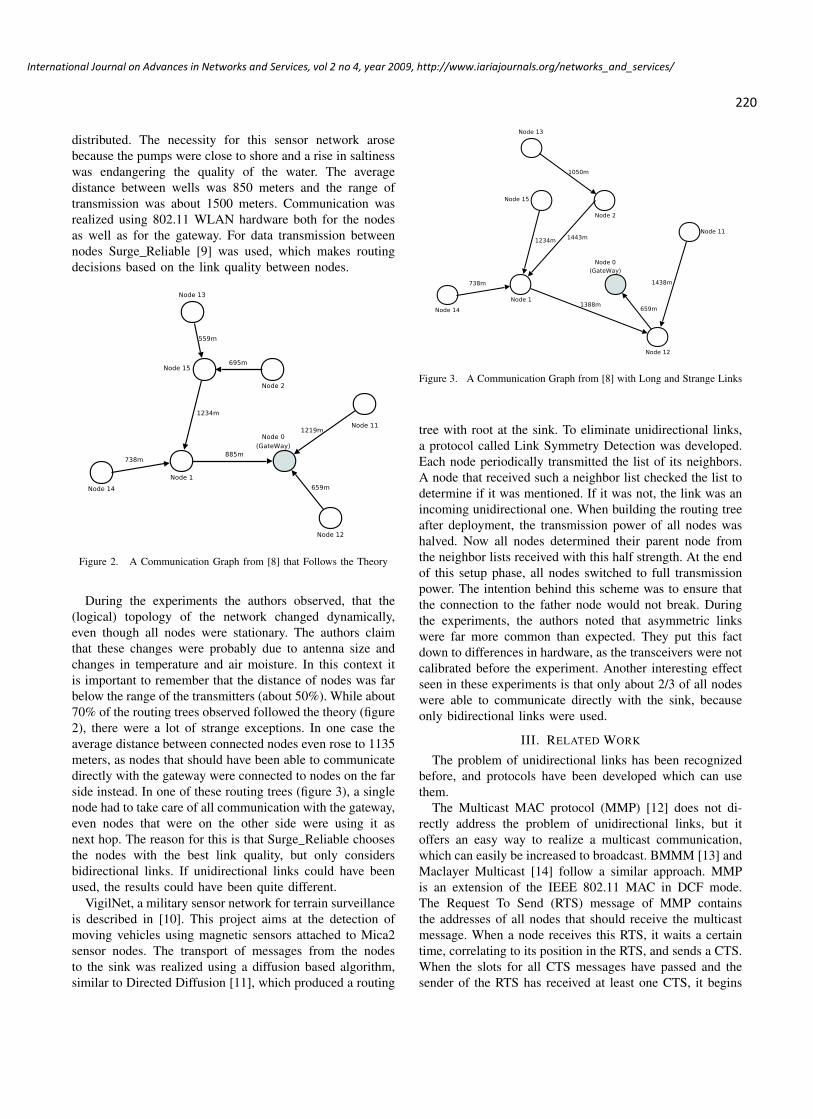
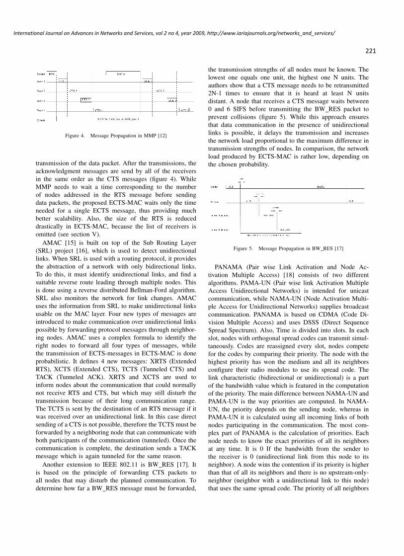
Figure 4. Message Propagation in MMP [12]
transmission of the data packet. After the transmissions, theacknowledgment messages are send by all of the receiversin the same order as the CTS messages (figure 4). WhileMMP needs to wait a time corresponding to the numberof nodes addressed in the RTS message before sendingdata packets, the proposed ECTS-MAC waits only the timeneeded for a single ECTS message, thus providing muchbetter scalability. Also, the size of the RTS is reduceddrastically in ECTS-MAC, because the list of receivers isomitted (see section V).
AMAC [15] is built on top of the Sub Routing Layer(SRL) project [16], which is used to detect unidirectionallinks. When SRL is used with a routing protocol, it providesthe abstraction of a network with only bidirectional links.To do this, it must identify unidirectional links, and find asuitable reverse route leading through multiple nodes. Thisis done using a reverse distributed Bellman-Ford algorithm.SRL also monitors the network for link changes. AMACuses the information from SRL to make unidirectional linksusable on the MAC layer. Four new types of messages areintroduced to make communication over unidirectional linkspossible by forwarding protocol messages through neighbor-ing nodes. AMAC uses a complex formula to identify theright nodes to forward all four types of messages, whilethe transmission of ECTS-messages in ECTS-MAC is doneprobabilistic. It defines 4 new messages: XRTS (ExtendedRTS), XCTS (Extended CTS), TCTS (Tunneled CTS) andTACK (Tunneled ACK). XRTS and XCTS are used toinform nodes about the communication that could normallynot receive RTS and CTS, but which may still disturb thetransmission because of their long communication range.The TCTS is sent by the destination of an RTS message if itwas received over an unidirectional link. In this case directsending of a CTS is not possible, therefore the TCTS must beforwarded by a neighboring node that can communicate withboth participants of the communication (tunneled). Once thecommunication is complete, the destination sends a TACKmessage which is again tunneled for the same reason.
Another extension to IEEE 802.11 is BW RES [17]. Itis based on the principle of forwarding CTS packets toall nodes that may disturb the planned communication. Todetermine how far a BW RES message must be forwarded,
the transmission strengths of all nodes must be known. Thelowest one equals one unit, the highest one N units. Theauthors show that a CTS message needs to be retransmitted2N-1 times to ensure that it is heard at least N unitsdistant. A node that receives a CTS message waits between0 and 6 SIFS before transmitting the BW RES packet toprevent collisions (figure 5). While this approach ensuresthat data communication in the presence of unidirectionallinks is possible, it delays the transmission and increasesthe network load proportional to the maximum difference intransmission strengths of nodes. In comparison, the networkload produced by ECTS-MAC is rather low, depending onthe chosen probability.
Figure 5. Message Propagation in BW RES [17]
PANAMA (Pair wise Link Activation and Node Ac-tivation Multiple Access) [18] consists of two differentalgorithms. PAMA-UN (Pair wise link Activation MultipleAccess Unidirectional Networks) is intended for unicastcommunication, while NAMA-UN (Node Activation Multi-ple Access for Unidirectional Networks) supplies broadcastcommunication. PANAMA is based on CDMA (Code Di-vision Multiple Access) and uses DSSS (Direct SequenceSpread Spectrum). Also, Time is divided into slots. In eachslot, nodes with orthogonal spread codes can transmit simul-taneously. Codes are reassigned every slot, nodes competefor the codes by comparing their priority. The node with thehighest priority has won the medium and all its neighborsconfigure their radio modules to use its spread code. Thelink characteristic (bidirectional or unidirectional) is a partof the bandwidth value which is featured in the computationof the priority. The main difference between NAMA-UN andPAMA-UN is the way priorities are computed. In NAMA-UN, the priority depends on the sending node, whereas inPAMA-UN it is calculated using all incoming links of bothnodes participating in the communication. The most com-plex part of PANAMA is the calculation of priorities. Eachnode needs to know the exact priorities of all its neighborsat any time. It is 0 If the bandwidth from the sender tothe receiver is 0 (unidirectional link from this node to itsneighbor). A node wins the contention if its priority is higherthan that of all its neighbors and there is no upstream-only-neighbor (neighbor with a unidirectional link to this node)that uses the same spread code. The priority of all neighbors
221
International Journal on Advances in Networks and Services, vol 2 no 4, year 2009, http://www.iariajournals.org/networks_and_services/
k in slot t is calculated as follows: ptk = bwk
√Rand(k + t)
where bwk is the bandwidth of node k. Rand is a randomfunction which delivers a number between 0 and 1. pk = 0if bwk = 0 In PAMA-UN the computation of the prioritydepends on all incoming links of both participating nodesx,y,: pt
(x,y) = bw(x,y)√
Rand(x + y + t). Both protocols,PAMA-UN and NAMA-UN depend on knowledge about the2-hop neighbors of a node. To determine this, a neighbor-hood protocol is used, which transmits updates about theneighborhood of a node regularly. Each node can computeits 2-hop neighborhood by combining these messages fromall its 1-hop neighbors. The update messages can containinformation about multiple links. This information containsthe ID of the neighbors, the status of the link (bidirectionalor unidirectional), the type of change (add or delete alink/neighbor) and the current bandwidth. Depending on therate of mobility the interval at which these messages are sentcan be adjusted.
IV. MLMAC-UL
In previous work we introduced MLMAC [19], [20], aTDMA based MAC protocol for mobile wireless sensornetworks. MLMAC divides time into frames, which are inturn divided into slots. Each node may use its own slot totransmit data to its neighbors, a slot reappears each frame.Nodes which have a common neighbor must have differentslots to prevent collisions. For static networks it is fairly easyto find a schedule for all nodes that fulfills this property, formobile nodes it is much harder. MLMAC uses an adaptiveapproach to enable each node in the sensor network toallocate a slot. In this approach there is no predefined starternode as in LMAC [21], rather the synchronization of nodesis started by the node that wants to transmit something first.
Figure 6. The Finite State Machine used in MLMAC [19]
In MLMAC a node may have one of 7 different states, andtransitions from one to the other under certain conditions.The complete state-machine can be seen in figure 6. Whennodes are first activated, MLMAC starts in the WAIT-state.
1) This node wants to transmit a message. It starts aglobal synchronization.
2) A control message from a node in STARTER- orREADY-state was received. Synchronize local time.
3) After listening for one frame, choose a slot.4) This nodes slot is active. Start transmitting a control
message every frame in this slot5) A collision seems to have occurred but the control
message was received on a unidirectional link.6) No collision occurred in the last frame.7) A collision seems to have occurred but the control
message was received on a unidirectional link.8) A collision occurred and the link to the sender is
bidirectional. Delete slot information.9) A collision occurred and the link to the sender is
bidirectional. Delete slot information.10) A control message with a different, older synchroniza-
tion was received. Remove all slot information.11) After waiting for a certain time, return to the beginning
and start again.
Most important for this work are the ready-state and thetransition to the sleep state.
A node that has reached the ready-state is in a stablestate, as long as no error occurs. If a collision occurs,the link from the sender is checked. If it is bidirectional,the node transitions into the sleep-state, because that isobviously wrong and a new slot has to be chosen. If thelink is unidirectional, the node remains in the ready-state. The determination, whether a link is unidirectional orbidirectional is realized with a simple counter. Whenevertransmissions are expected but not received, this counter ischanged. After a predetermined number of missed messages,the link is considered unidirectional. This method has provento be too ineffective for our purpose.
In this section we introduce the changes we made toMLMAC, to stop only detecting unidirectional links andignore collisions that occurred because of them. Rather,MLMAC-UL uses a neighborhood discovery protocol todetermine neighbors that can be used to inform the originatorof a unidirectional link (the node that can be heard by theother one) about the link and make it usable to forwardmessages.
The first addition is an independent neighborhood discov-ery protocol, which is similar to the ones used in AMAC[15] and PANAMA [18] (see Section III). It transmits theneighborhood table of a node periodically but seldom. Inthe case of changes, only small update messages are sent.The periodic sending of tables is used to remove any errorsresulting from loss of update packets.
222
International Journal on Advances in Networks and Services, vol 2 no 4, year 2009, http://www.iariajournals.org/networks_and_services/

Another change in MLMAC-UL is the fact that nodescan give up their slots. If a node has transmitted only statusmessages for a certain time (e.g., 6 frames) it will inform itsneighbors that it is giving up the slot and that it may be usedby another node. This is done by altering the status messagea node transmits at the beginning of its slot. Moreover, anode may not only hold one slot in MLMAC-UL. Rather,each node can use as many slots as it needs by claimingany unused ones, when it has to transmit lots of data. Oncethe send queue is emptied, it can give the additional slotsup one after the other. For this to be effective it is useful todefine a larger frame size from the beginning, so that thereare always enough free slots available (figure 7). This abilityto hold more slots was introduced to reduce the delay andmake MLMAC a better competitor against contention basedprotocols.
Figure 7. Using different Frame Sizes
Each node maintains a list of all its neighbors. Threeentries define this list: The link quality, the unidirection-ality status and the compressed neighborhood informationfrom that neighbor. The link quality can be good (morethan 90%reception rate), medium (between 30% and 90 %reception rate) or bad (less than 30% reception rate). Theunidirectionality status can be either bidirectional, unidi-rectional sender or unidirectional receiver. The compressedneighborhood list is maintained by the neighborhood discov-ery protocol and used to identify the 2-hop-neighborhood ofthe current node.
The state machine of MLMAC-UL can be seen in figure8. The arrows in the figure represent the transitions betweenstates and are described in the following.
1) When a node needs to acquire its first slot it switchesinto the state UNSYNC.
2) The node was in state UNSYNC for one frame. Itchooses a slot and transitions into the SYNC-state. Ifno slot was empty, the node stays in its current statefor another frame.
3) When its chosen slot arrives, the node changes to stateSLOTVERIFY.
4) The node sends in its slots. After one frame, it reachesthe READY- state.
5) If a negative acknowledgment for the last slot wasreceived, the slot is deleted and the node changes tostate SLEEP.
Figure 8. The State Machine of MLMAC-UL
6) The node returns to the WAIT-state after a randomamount of time.
7) Same as 5.8) There is data to be transmitted and no neighboring
node is transmitting. The node chooses a slot and anidentification for the synchronization. After waiting fora random time it transmits the data and switches toREADY.
9) If this node did not communicate before or it hadpreviously given up one slot a new slot is acquiredand the node changes into the state SLOTVERIFY.
10) No messages from neighbors were received for 5frames even though this node is transmitting. Thismeans that this node is either completely isolated,or has only unidirectional links to others, but noincoming link from any of them. This node switches tothe ALONE-state and does not try to transmit anymore,even when data is available.
11) A message from a neighbor was received, whichmeans that this node is no longer alone or a certainnumber of frames (e.g., 200) have passed. The nodeswitches to WAIT and starts again.
V. ECTS-MAC
ECTS-MAC (Extended Clear To Send MAC) is a con-tention based protocol for sparse networks with rare com-munication. It is similar to BW RES [17] (see SectionIII), because it also tries to forward the CTS message toreduce the probability of collision. Unlike BW RES, itdoes not calculate distances and power levels. Also, allECTS messages are sent at the same time, whereas allBW RES messages are sent one after another. This leadsto more collisions of ECTS messages, but saves a lot oftime. When a node receives a CTS message it forwardsit with a certain probability (figure 9). Experiments haveshown that 50% seems to be the optimal value for sparsenetworks. If the probability is less, the ECTS message is
223
International Journal on Advances in Networks and Services, vol 2 no 4, year 2009, http://www.iariajournals.org/networks_and_services/

not received by enough neighbors. If it is higher, the ECTSpackets collide more often. These collisions are also thereason why the ECTS-MAC should only be used in sparsenetworks, as the ECTS packets would increase the networkload in a dense network too much. To a certain extend, thiseffect is alleviated by reducing the probability of sending,but this also leads to more nodes that do not receive theECTS message. The ECTS-MAC uses the neighborhooddiscovery protocol described in the previous section to detectunidirectional links. This is necessary to enable transmittingvia a unidirectional link, because acknowledgments need tobe forwarded to the sender using a second node.
Figure 9. Propagation of ECTS Messages
VI. EVALUATION
To measure the performance of MLMAC-UL and ECTS-MAC, we evaluated them against two other protocols: Theoriginal MLMAC and a modified version of MMP (MulticastMac Protocol) [12] (see Section III). As its name suggests,MMP was designed for multicast, not for broadcast. Wechanged its behavior to enable broadcast transmissions, andto enable it to use unidirectional links. For this, we onceagain used the neighborhood discovery protocol describedabove. We call the resulting protocol NMAC (NeighborhoodMAC). The functionality of NMAC is depicted in figure 10.Because of the neighborhood discovery protocol, the nodeknows how many neighbors it has and addresses them allin the RTS packet. When a node receives a RTS messageit waits for a time corresponding to its position in the RTSbefore transmitting a CTS. If it has received at least oneCTS, the sender of the RTS transmits the data package afterthe time for all CTS messages has passed.
Figure 10. Message Propagation in NMAC
For our evaluations we used the discrete event simulatorOMNeT++ [22] as well as real sensornet hardware. In all
simulations the nodes transmitted with 19.2 KBit per secondand a transmission strength of 10 milliwatt. For our realexperiments we used TMote Sky sensor nodes from MoteIVcorporation. These feature a MSP430 microcontroller witha frequency of 8MHz, 10 kB of Ram and 48 kB of flash.The radio module is IEEE 802.15.4 compatible and transmits250kB/s, we configured the transmission strength to -25dBmto enable a multi hop scenario.
A. Single Hop Scenario Simulation
In this scenario the application behavior for a direct one-hop-neighborhood was simulated. The application tried tosend as fast as possible. It generated a packet with 110bytes data every 20 milliseconds, up to a total of 500packets. In this simulation, all 4 protocols achieved a packetreception rate of nearly 100%. Figure 11 shows the amountof application data transmitted by each protocol. The figureshows that for 2-4 nodes the contention based protocols areable to transmit more data than the TDMA protocols. Whenmore nodes are used, MLMAC-UL can gain an advantagebecause of the usage of multiple slots per node. As thenumber of slots was not changed for the MLMAC, it alwaysdelivers the same amount of data.
Figure 11. Data Transmitted 1-Hop Scenario
B. High Load Scenario Simulation
In this scenario a rectangle of 6 time 8 nodes wassimulated. The application tried to send as fast as possi-ble. It generated a packet with 110 bytes data every 20milliseconds, up to a total of 500 packets. The node inthe upper left corner started transmitting, each other nodebegan transmitting its 500 packets after it had received thefirst packet. From a certain time on, all nodes want totransmit at nearly the same time, thus leading to a high
224
International Journal on Advances in Networks and Services, vol 2 no 4, year 2009, http://www.iariajournals.org/networks_and_services/

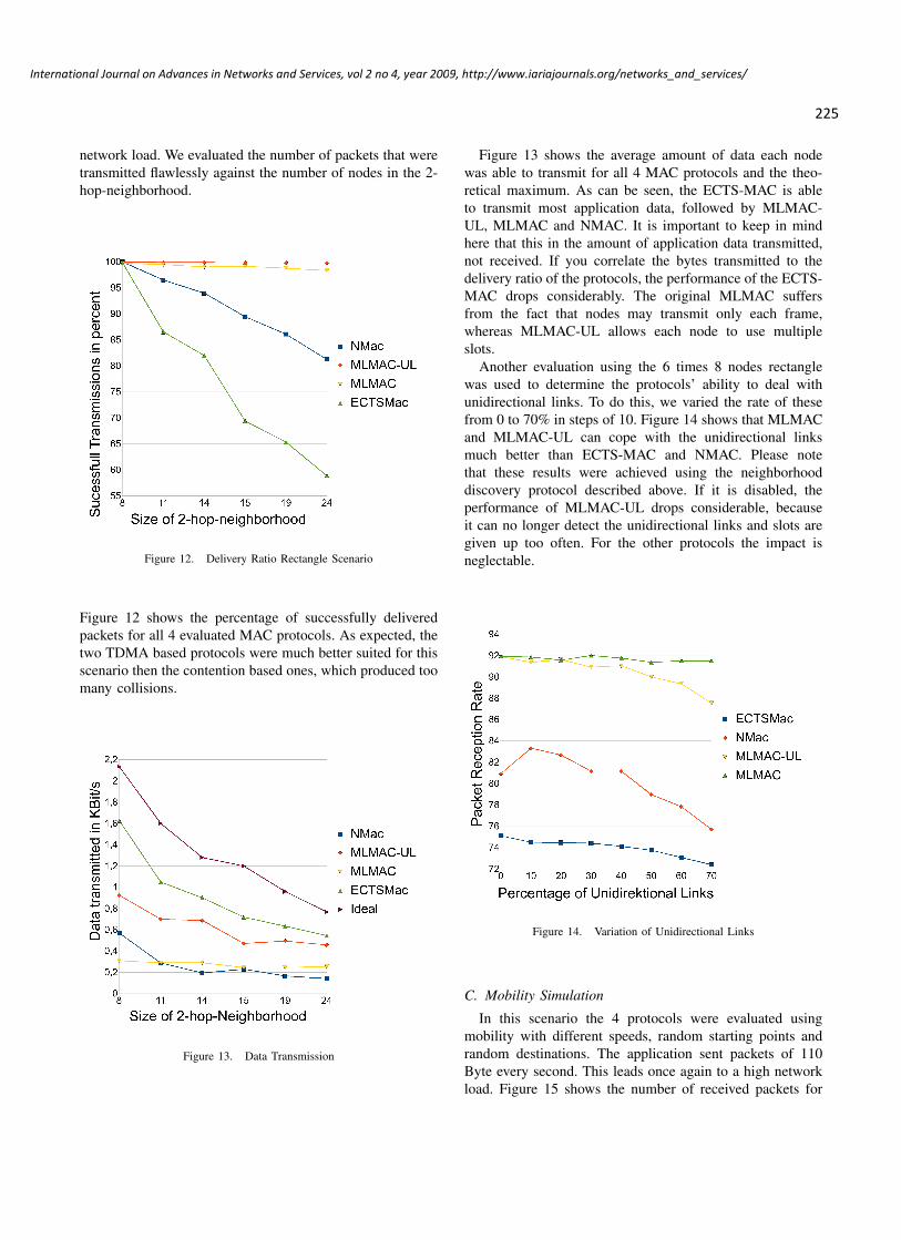
network load. We evaluated the number of packets that weretransmitted flawlessly against the number of nodes in the 2-hop-neighborhood.
Figure 12. Delivery Ratio Rectangle Scenario
Figure 12 shows the percentage of successfully deliveredpackets for all 4 evaluated MAC protocols. As expected, thetwo TDMA based protocols were much better suited for thisscenario then the contention based ones, which produced toomany collisions.
Figure 13. Data Transmission
Figure 13 shows the average amount of data each nodewas able to transmit for all 4 MAC protocols and the theo-retical maximum. As can be seen, the ECTS-MAC is ableto transmit most application data, followed by MLMAC-UL, MLMAC and NMAC. It is important to keep in mindhere that this in the amount of application data transmitted,not received. If you correlate the bytes transmitted to thedelivery ratio of the protocols, the performance of the ECTS-MAC drops considerably. The original MLMAC suffersfrom the fact that nodes may transmit only each frame,whereas MLMAC-UL allows each node to use multipleslots.
Another evaluation using the 6 times 8 nodes rectanglewas used to determine the protocols’ ability to deal withunidirectional links. To do this, we varied the rate of thesefrom 0 to 70% in steps of 10. Figure 14 shows that MLMACand MLMAC-UL can cope with the unidirectional linksmuch better than ECTS-MAC and NMAC. Please notethat these results were achieved using the neighborhooddiscovery protocol described above. If it is disabled, theperformance of MLMAC-UL drops considerable, becauseit can no longer detect the unidirectional links and slots aregiven up too often. For the other protocols the impact isneglectable.
Figure 14. Variation of Unidirectional Links
C. Mobility Simulation
In this scenario the 4 protocols were evaluated usingmobility with different speeds, random starting points andrandom destinations. The application sent packets of 110Byte every second. This leads once again to a high networkload. Figure 15 shows the number of received packets for
225
International Journal on Advances in Networks and Services, vol 2 no 4, year 2009, http://www.iariajournals.org/networks_and_services/
each protocol for the different speeds. Once again, MLMACand MLMAC-UL provide the best results, with ECTS-MACperforming only a little worse. The strong problems ofNMAC are the result of a high rate of collisions. This isdue to the fact that nodes which are leaving each othersvicinity and thus produce a high number of transmissionerrors are seen as unidirectional links by both nodes andthus not addressed in the RTS message. They don’t forwardthe CTS, which leads to another rise in collisions. Theproblem gets worse when nodes re-enter each others vicinityshortly after leaving it, because their links remain markedas unidirectional too long.
Figure 15. Received Packets
D. Simulated Flooding over 50 hops
In this set of simulations, the performance under lownetwork load is evaluated. We simulated a line of 6 to 51nodes, where each node was only able to communicate withits direct neighbors. Table II shows the time needed by eachprotocol to deliver a message over 50 hops. The times forthe TDMA protocols are divided once using 5 slots and onceusing 31. Even though there were enough unused slots, theMLMAC-UL did not acquire new ones, because there wasnot much data to be sent and the send queue only ever heldone packet. This leads to nearly the same time (one frame)needed as when using the original MLMAC, as the timefor one hop only depended on the frame length. For allprotocols, the time needed to reach the last node increasedlinearly with the number of nodes in use.
Table IITIME NEEDED FOR 50 HOPS (MS)
NMAC 3,77MLMAC-UL 31 slots 70,29MLMAC 31 slots 69,25ECTS-Mac 3,63MLMAC-UL 5 slots 12,32MLMAC 5 slots 10,79
E. Packet Overhead
This last evaluation in the simulator was based on thesame topology as the high load scenario, but the size of thedata generated by the application was varied between 20 and110 Byte. It transmitted at random intervals between 0 and5000 milliseconds. Figure 16 shows the relative overheadeach protocol produced (protocol bytes/total bytes) for anincreasing size of the 2-hop-neighborhood. The calculationincludes the periodic messages from the TDMA basedprotocols and the RTS, CTS and ECTS messages fromthe contention based protocols. It can be seen that NMACproduces by far the highest overhead, followed by the ECTS-MAC. Thus, contrary to common belief, sending periodicstatus messages does not produce a high overhead.
Figure 16. Protocol Overhead
F. Direct Neighborhood Experiments
In these experiments the application sent 500 packets ofsize 110 Byte every 10 Milliseconds. They were performedusing 3, 7, 11 and 16 nodes. Figure 17 shows that for asmall number of nodes all protocols perform relatively well.With an increasing number of nodes the performance of firstNMAC and then MLMAC drop considerably. This is due to
226
International Journal on Advances in Networks and Services, vol 2 no 4, year 2009, http://www.iariajournals.org/networks_and_services/

the increased number of CTS and ECTS messages, whichlead to a high network load, a lot of collisions and thus alow throughput.
Figure 17. Packet Delivery Ratio Single Hop Experiments
G. High Load Scenario Experiments
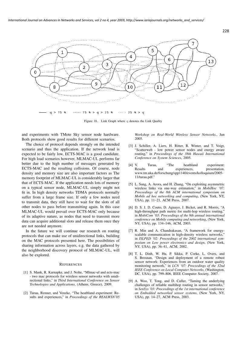
For these experiments we placed 14 TMote Sky sensornodes on the floor in a building. As there are no waysto define link quality in a real experiment we could onlymeasure it. Figure 18 shows the resulting communicationgraph. It can be seen that the radio neighborhood of thenodes and the link quality differ a lot.
The application was once again the one producing thehigh network load. The left side of Figure 19 shows theaverage time needed to transmit one packet. MLMAC-UL and ECTS-MAC were the fastest ones, with MLMACfollowing and NMAC bringing up the rear. On the right sideof the figure you can see the total number of received packetsfor each protocol. All protocols received nearly the sameamount of messages, with only NMAC being considerablybetter
But this fact has to be put in perspective: all 4 protocols wereevaluated one after another, using the same nodes and, mostimportant, the same batteries. NMAC was the first protocolto be evaluated, which means that is had the advantage offresh batteries which have been shown to have a positiveeffect on the range of the transceivers and thus link quality.
Figure 19. Time to Send(l) and Number of received Packets(r)
H. Memory Consumption
On Figure 20 the memory consumption of the protocolsis shown, with 3 slots for the TDMA protocols on the leftand 16 slots on the right. It is also differentiated whetherthe neighborhood discovery protocol was used or not, onlythe original MLMAC is shown only once, because it neveruses that protocol. Please note that the numbers shown arefor RAM consumption, the usage of flash memory followsthe same distribution. On the figure it can be seen thatMLMAC-UL needs most memory and ECTS has the lowestmemory consumption. Combining this fact with the otherresults leads to the observation that for networks with lowmemory allowance and few nodes the ECTS-MAC shouldbe chosen while the MLMAC-UL is best suited for densernetworks with high load.
Figure 20. Memory Consumption for 3(l) and 16 Slots(r)
VII. CONCLUSION AND FUTURE WORK
In this paper we have discussed the influence of unidi-rectional links on communication protocols. We presentedtwo MAC protocols that can utilize unidirectional linksto increase network connectivity, reliability and lifetime.MLMAC-UL is an enhancement to MLMAC, a TDMAbased protocols for wireless sensor networks. ECTS-MACis a contention based protocol that informs nodes that areconnected to a sending node through unidirectional linksabout the impending communication by forwarding theCTS messages through multiple hops. Both protocols wereevaluated by comparison with other protocols in simulations
227
International Journal on Advances in Networks and Services, vol 2 no 4, year 2009, http://www.iariajournals.org/networks_and_services/
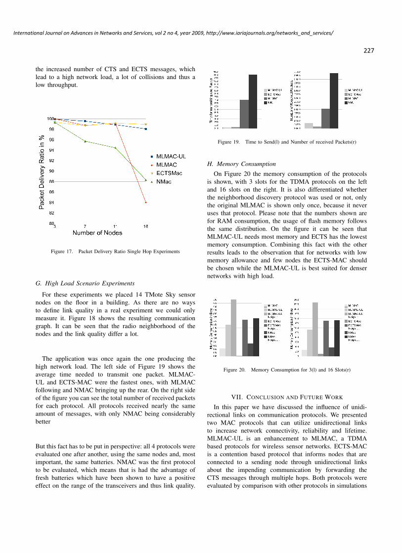
Figure 18. Link Graph where q denotes the Link Quality
and experiments with TMote Sky sensor node hardware.Both protocols show good results for different scenarios.
The choice of protocol depends strongly on the intendedscenario and thus the application. If the network load isexpected to be fairly low, ECTS-MAC is a good candidate.For high load scenarios however, MLMAC-UL performs farbetter due to the high number of messages generated byECTS-MAC and the resulting collisions. Of course, nodedensity and memory size are also important factors as Thememory footprint of MLMAC-UL is considerably larger thatthat of ECTS-MAC. If the application needs lots of memoryon a typical sensor node, MLMAC-UL simply might notfit in. In high density networks TDMA protocols normallysuffer from a large frame size. If only a few nodes needto transmit data, they still have to wait for the slots of allother nodes to pass before transmitting again. In this caseMLMAC-UL would prevail over ECTS-MAC only becauseof its adaptive nature, as nodes that need to transmit moredata can acquire additional slots and release them once theyare not needed anymore.
In the future we will continue our research on routingprotocols that can make use of unidirectional links, buildingon the MAC protocols presented here. The possibilities ofsharing information across layers, e.g. the data gathered bythe neighborhood discovery protocol of MLMAC-UL, willalso be explored.
REFERENCES
[1] S. Mank, R. Karnapke, and J. Nolte, “Mlmac-ul and ects-mac- two mac protocols for wireless sensor networks with unidi-rectional links,” in Third International Conference on SensorTechnologies and Applications, (Athens, Greece), 2009.
[2] Turau, Renner, and Venzke, “The heathland experiment: Re-sults and experiences,” in Proceedings of the REALWSN’05
Workshop on Real-World Wireless Sensor Networks., Jun2005.
[3] J. Schiller, A. Liers, H. Ritter, R. Winter, and T. Voigt,“Scatterweb - low power sensor nodes and energy awarerouting,” in Proceedings of the 38th Hawaii InternationalConference on System Sciences, 2005.
[4] V. Turau, “The heathland experiment:Results and experiences, presentation.www.tm.uka.de/forschung/spp1140/events/kolloquium/2005-11/turau.pdf.”
[5] L. Sang, A. Arora, and H. Zhang, “On exploiting asymmetricwireless links via one-way estimation,” in MobiHoc ’07:Proceedings of the 8th ACM international symposium onMobile ad hoc networking and computing, (New York, NY,USA), pp. 11–21, ACM Press, 2007.
[6] D. S. J. D. Couto, D. Aguayo, J. Bicket, and R. Morris, “Ahigh-throughput path metric for multi-hop wireless routing,”in MobiCom ’03: Proceedings of the 9th annual internationalconference on Mobile computing and networking, (New York,NY, USA), pp. 134–146, ACM, 2003.
[7] R. Min and A. Chandrakasan, “A framework for energy-scalable communication in high-density wireless networks,”in ISLPED ’02: Proceedings of the 2002 international sym-posium on Low power electronics and design, (New York,NY, USA), pp. 36–41, ACM, 2002.
[8] T. L. Dinh, W. Hu, P. Sikka, P. Corke, L. Overs, andS. Brosnan, “Design and deployment of a remote robustsensor network: Experiences from an outdoor water qualitymonitoring network,” in LCN ’07: Proceedings of the 32ndIEEE Conference on Local Computer Networks, (Washington,DC, USA), pp. 799–806, IEEE Computer Society, 2007.
[9] A. Woo, T. Tong, and D. Culler, “Taming the underlyingchallenges of reliable multihop routing in sensor networks,”in SenSys ’03: Proceedings of the 1st international conferenceon Embedded networked sensor systems, (New York, NY,USA), pp. 14–27, ACM Press, 2003.
228
International Journal on Advances in Networks and Services, vol 2 no 4, year 2009, http://www.iariajournals.org/networks_and_services/
[10] T. He, S. Krishnamurthy, L. Luo, T. Yan, L. Gu, R. Stoleru,G. Zhou, Q. Cao, P. Vicaire, J. A. Stankovic, T. F. Abdelzaher,J. Hui, and B. Krogh, “Vigilnet: An integrated sensor networksystem for energy-efficient surveillance,” ACM Trans. Sen.Netw., vol. 2, no. 1, pp. 1–38, 2006.
[11] C. Intanagonwiwat, R. Govindan, D. Estrin, J. Heidemann,and F. Silva, “Directed diffusion for wireless sensor network-ing,” IEEE/ACM Trans. Netw., vol. 11, no. 1, pp. 2–16, 2003.
[12] H. Gossain, N. Nandiraju, K. Anand, and D. P. Agrawal,“Supporting mac layer multicast in ieee 802.11 based manets:Issues and solutions,” in LCN ’04: Proceedings of the 29thAnnual IEEE International Conference on Local ComputerNetworks, (Washington, DC, USA), pp. 172–179, IEEE Com-puter Society, 2004.
[13] R. M. Yadumurthy, A. C. H., M. Sadashivaiah, and R. Makan-aboyina, “Reliable mac broadcast protocol in directionaland omni-directional transmissions for vehicular ad hoc net-works,” in VANET ’05: Proceedings of the 2nd ACM interna-tional workshop on Vehicular ad hoc networks, (New York,NY, USA), pp. 10–19, ACM, 2005.
[14] S. Jain and S. R. Das, “Mac layer multicast in wirelessmultihop networks.,” in COMSWARE ’06: Proceedings ofthe 1st International Conference on Communication SystemSoftware and Middleware, 2006.
[15] G. Wang, D. Turgut, L. Boloni, Y. Ji, and D. C. Marinescu, “Asimulation study of a mac layer protocol for wireless networkswith asymmetric links,” in IWCMC ’06: Proceedings of the2006 international conference on Wireless communicationsand mobile computing, (New York, NY, USA), pp. 929–936,ACM, 2006.
[16] V. Ramasubramanian, R. Chandra, and D. Mosse, “Providinga bidirectional abstraction for unidirectional ad hoc net-works,” 2002.
[17] N. Poojary, S. V. Krishnamurthy, and S. Dao, “Mediumaccess control in a network of ad hoc mobile nodes withheterogeneous power capabilities,” in in: IEEE InternationalConference on Communications (ICC), 2001, pp. 872–877,2001.
[18] L. Bao and J. J. Garcia-Luna-Aceves, “Channel accessscheduling in ad hoc networks with unidirectional links,” inDIALM ’01: Proceedings of the 5th international workshopon Discrete algorithms and methods for mobile computingand communications, (New York, NY, USA), pp. 9–18, ACM,2001.
[19] S. Mank, R. Karnapke, and J. Nolte, “An adaptive tdma basedmac protocol for mobile wireless sensor networks, best paperaward,” in International Conference on Sensor Technologiesand Applications, 2007.
[20] S. Mank, R. Karnapke, and J. Nolte, “Mlmac - an adaptivetdma mac protocol for mobile wireless sensor networks,”in Ad-Hoc & Sensor Wireless Networks: An InternationalJournal, Vol.8 Nr.1-2, 2009.
[21] L. van Hoesel and P. Havinga, “A lightweight medium ac-cess protocol (lmac) for wireless sensor networks: Reducingpreamble transmissions and transceiver state switches,” inINSS, Japan, Jun 2004.
[22] A. Varga, “The omnet++ discrete event simulation system,”in Proceedings of the European Simulation Multiconference(ESM’2001), (Prague, Czech Republic), June 2001.
229
International Journal on Advances in Networks and Services, vol 2 no 4, year 2009, http://www.iariajournals.org/networks_and_services/

A Novel Fault Diagnosis Technique in Wireless Sensor Networks
Anas Abu Taleb, J. Mathew and D.K. Pradhan Department of Computer Science
University of Bristol Bristol, UK
{ abutaleb, jimson, pardhan} @cs.bris.ac.uk
Taskin Kocak Department of Computer Engineering
Bahcesehir University Istanbul, Turkey
Abstract—In sensor networks, per formance and reliability depend on the fault tolerance scheme used in the system. With increased network size traditional fault tolerant techniques have proven inadequate. Fur ther , identifying and isolating the fault is one of the key steps towards reliable network design. Towards this, we propose two new algor ithms to detect and substitute faulty nodes at different levels in the network. In the proposed approach, the network is divided into zones which are having a master for each zone. Moreover , the masters of the zones are connected in a De Bruijn graph based network. When a fault occurs, the masters are checked, tested. After that, the sensor nodes in the suspected zone are tested. Our fault model assumes communication, processing and sensing faults caused by hardware failures in a node. We analyzed the per formance of the first algor ithm according to the number of messages it needs to diagnose faulty nodes. In addition, the per formance of a 4-node De Bruijn graph was also studied by measur ing the end-to-end delay. Finally, the per formance of the second algor ithm was studied by measur ing the fault detection accuracy.
Keywords- Wireless Sensor Networks, Fault Tolerance, Fault Diagnosis, De Bruijin Graph
I. INTRODUCTION
The advances in wireless communication and electronics made it possible to develop low-cost sensor nodes, which can be deployed easily in specific areas in order to accomplish a specific mission by forming a wireless sensor network (WSN). It might be difficult or dangerous for humans to enter these areas because nodes in this type of networks are expected to operate in inhospitable environments [2]. Therefore, sensor nodes are expected to operate for periods ranging from days to years without any human intervention. There is a tremendous need for fault tolerant WSNs because, sensor nodes are subject to various types of failures and faults such as communication, processing and sensing faults.
A sensor network must be capable of identifying and replacing the faulty nodes in order to make sure that the network’s quality-of-service (QoS) is maintained. Identifying faulty sensor nodes is not an easy task as it is difficult and time consuming for the base station to keep the information about all the sensor nodes in the network. When addressing fault tolerance in WSNs, three types of node failures must be taken into account. First, when the sensor node is faulty and
not providing data. Second, when the node processes data erroneously. Third, occurs when we have an active node that is providing incorrect data.
In this paper, we propose a new technique consisting of two algorithms to identify faults occurring at different levels or places in the network, i.e. faults that occur at the zones masters and the sensor nodes associated with the zones masters. The proposed technique divides the network into disjoint zones while having a master for each zone. When a fault occurs, the first algorithm is triggered to test the masters. The technique will not trigger the second algorithm unless all the masters are diagnosed fault free by the first algorithm. Thus, when the second algorithm is triggered, the master of the suspected zone is responsible for identifying the suspected faulty nodes. As a result, the master will start searching for sleeping nodes to wake up and depending on the reading it gets from the suspected and awakened nodes, the master can decide whether the suspected nodes are faulty or not, moreover, it can decide on which node to switch off. A preliminary version of this paper is published in [1], in which a technique to detect faulty sensor nodes was presented.
The paper is organized as follows. In section II the related work is reviewed. Then the concept of De Bruijn graph is discussed and explained in section III. In section IV, the network architecture and the fault model are defined. In section V the proposed technique is described. Section VI describes the simulator used and illustrates the simulated scenarios. Also, we use an example of a potential chemical spill to describe various concepts. The simulation results are also reported in this section. Finally the paper is concluded in section VII.
II. RELATED WORK
Several works have addressed the problem of how to deal with faults occurring in wireless sensor networks in order to achieve fault tolerance [3][4][5]. These researches consider the faults that result from sensor nodes failures, which affect the network connectivity and coverage. The research proposed in [3], makes use of redundancy and uses a technique to decide on which nodes to keep active and on which to put in a sleep mode. The technique aims to provide the sensor field with the best possible coverage. In addition, it maintains network connectivity to route information. When an active node fails it is substituted by one of the sleeping nodes. However, other researchers have addressed
230
International Journal on Advances in Networks and Services, vol 2 no 4, year 2009, http://www.iariajournals.org/networks_and_services/
the problem of having active nodes that provide incorrect data which results in making inappropriate decisions. The research proposed in [4] focused on such issues and proposed a mechanism to detect and diagnose data in consistency failures in wireless sensor networks.
The mechanism proposed in [4] uses two disjoint paths to send the sensed data to a static sink. After the sink receives both copies, it will compare them to check if they match. If the two copies match, both the data and the paths are considered to be fault free otherwise, a third disjoint path will be established. Then, the sensor node will send three copies on the three disjoint paths to the sink. The sink will compare these copies and decides on the faulty path. Finally, a diagnosis routine will be executed to identify the faulty node within the faulty path.
Another research has taken fault tolerance in account, so that to achieve fault tolerance the sensor network is partitioned into distinct clusters and the node that has the highest energy level is selected to be the cluster head where only cluster heads are allowed to communicate with the base station [5]. Therefore, they introduced a two-phase fault tolerant approach which consists of detection and recovery where the status of the cluster heads is checked periodically. Sensors associated with a faulty cluster head are recovered by joining them to another cluster [5].
The research described in [6] proposed a scheme based on multi-path routing combined with channel coding to achieve fault tolerance. It uses a fuzzy logic based algorithm that is energy and mobility aware to select multiple paths. When selecting the paths, the algorithm takes the remaining energy, mobility and the distance to the destination into account. Another research has proposed a design for a system to diagnose the roots of faults occurring in wireless sensor networks. The authors have proposed an algorithm to diagnose the cause of faults in which the behavior of sensor nodes in monitored locally. The diagnosis procedure will be triggered when a node detects a strange behavior [7]. In [8], a general framework to achieve fault tolerance in wireless sensor networks was proposed. The framework is based on a learning and refinement module which provides adaptive and self-configurable solutions.
A localized algorithm for fault detection to identify faulty sensors that is based on having neighbor sensor nodes testing each other was proposed in [9]. In [10], an efficient algorithm to trace failed nodes in sensor networks was proposed. In addition, they demonstrate that if the network topology is conveyed efficiently to the base station, it allows tracing the failed entities quickly with moderate communication overhead.
In [11], the authors proposed fault tolerant algorithms to detect the region of an event in wireless sensor networks. Also, they assume that nodes report a binary decision to indicate the presence of an event or not and considered a byzantine behavior for the faulty nodes, which means that the faulty nodes will be providing arbitrary values. Hence, they proposed a randomized decision scheme and a threshold decision scheme which a sensor node can use to decide on which binary decision to send by comparing the decision it has with the decisions of its neighbors
In [12], a fault map was constructed using a fault estimation model. In order to build the fault map, sensor nodes are required to send additional information that can be used by the fault estimation model. Furthermore, a cluster based algorithm to estimate faults in wireless sensor networks was proposed. In [13], a target detection model for sensor networks was proposed. In addition, two algorithms to facilitate fault tolerant decision making were presented. The first algorithm is based on collecting the actual readings from the neighboring nodes. In the second algorithm, the sensor node obtains the decisions made by the other neighboring nodes to take a final decision.
A distributed cluster based fault tolerant algorithm was proposed in [14]. The cluster head sends a small packet to indicate that it is still alive. Hence, a sensor node in the same cluster listens to the transmissions of its neighbors and to that of the cluster head. When a sensor node does not receive the short packets sent by the cluster head, it will trigger fault detection. Depending on the number of nodes that have not heard from the cluster head, it can be decided whether the cluster head is faulty, as the faulty node can be a member of the cluster and not the cluster head itself. If the cluster head was faulty, the cluster members will select a new cluster head. The authors in [15] apply error correcting codes to achieve fault tolerance. As a result, a distributed fault tolerant classification approach was proposed. The approach proposed is base of fault tolerant fusion rules that are used to obtain local decision rules at every sensor. In addition, the authors proposed two algorithms that can be used to find good code matrices to be used by the classification approach.
The work proposed in this paper differs from that presented by other researches in two aspects. First, the mechanism according to which sleeping nodes are activated to test active node. Second, the reading of neighboring nodes i.e. nodes covering the same terrain, are needed and compared only when the network is suspected to contain faulty nodes.
Moreover, we compare the performance of our work to the performance of the work presented in [11] because both techniques make use of neighboring nodes to detect a fault. In addition, no restriction on the number of neighboring nodes is imposed. Also, both techniques make use of threshold in their operation.
III. DE BRUIJN GRAPH
Part of the work proposed in this paper is based on constructing a De Bruijn graph based network at the zones masters level. This graph has interesting properties that make it important to investigate its use in WSNs. The degree of this graph is bounded, which means the degree of the network remains fixed even when the network size increases. In addition, this graph has interesting properties such as small diameter, high connectivity and easy routing. Furthermore, De Bruijn graph contains some important networks such as ring. Regarding fault tolerance and extensibility, these graphs maintain a good level of fault tolerance and self-diagnosability. For instance, in the presence of a single fault in the network, it takes four additional hops to detour around the faulty node and the
231
International Journal on Advances in Networks and Services, vol 2 no 4, year 2009, http://www.iariajournals.org/networks_and_services/
control information needed to do so can be integrated locally between the faulty node’s neighbors. Also, De Bruijn graph is extensible in two methods that are described in [18].
As a result, it will be interesting to investigate the used of De Bruijn graphs in sensor networks in order to increase the fault tolerance capabilities. In other words, if some nodes in the network were deployed according to De Bruijn graph, the network will have the ability to tolerate the presence of faulty nodes in the network and remain functional. In this work, the zone masters are assumed to be connected according a De Bruijn graph. The network assumed to be working if a zone master fails and the rest of the nodes in network will remain functional and the fault free zone master are capable of communicating with each other. Thus, accomplishing the network mission until the problem in the network is resolved.
The De Bruijn graph denoted as DB(r, k) has krN = nodes with diameter k and degree 2r. This corresponds to the state graph of a shift register of length k using r-ary digits. A shift register changes a state by shifting in a digit in the state number in one side, and then shifting out one digit from the other side. If we represent a node by
)...,,( 0121 iiiiI KK −−= where )1(,...,1,0 −∈ ri ,
( )10 −≤≤ kj , then its neighbors are represented by
piii kk 032 ...,,−− and 121 ,...,iipi kk −− , where
( )1,...,1,0 −= rp . The DB(2, k), which is called binary De Bruijn graph, can be obtained as follows. If we represent
a node I by a k-bit binary number, say, 0121 ...,, iiiiI kk −−= ,
then its neighbors can be presented as 0...,, 012 iiik− ,
1...,, 012 iiik− , 121 ...,,0 iii kk −− , and 021 ...,,1 iii kk −− .
IV. NETWORK ARCHITECTURE AND FAULT MODEL
We assume that the network is densely deployed and consists of heterogeneous nodes; which means that in addition to the ordinary sensor nodes, the network consists of some nodes that are more energy rich than others. The energy rich nodes are placed or deployed in a way that guarantees them to form a De Bruijn based network, while the rest of the nodes are deployed randomly. Also, the network has most of the nodes awake and a small number of nodes are in a sleep status. The nodes are fully static and the network is divided into four zones. In each zone the active node with the highest energy level will be chosen to be the zone master, for example in the shaded zone in Fig.1 the zone master is node 9, where the dark dots are the active nodes. After that, the master acts as a data sink and will be responsible for identifying faulty nodes in its zone while the remaining nodes in a zone can only send the sensed data to their master.
After being elected as zones maters for their zones, the zone masters communicate among themselves. In other words, each zone master knows the neighboring zone masters in the neighboring zones. Hence, a De Bruijn graph based network, consisting of the zone masters only, is
constructed. This graph has interesting properties that assist in increasing fault tolerance capabilities of the network. Figure 2 shows the DB(2,2) De Bruijn Graph.
Figure 1. The Network Architecture. After constructing the De Bruijn based network, when a
zone is suspected to contain faulty nodes, the master of that zone will be tested and diagnosed using the distributed fault diagnosis algorithm described in section V. If the zone master is faulty, it will be substituted by one of its neighboring sleeping nodes, as a result, the De Bruijn based network will not need to be constructed again. On the other hand, if the master was fault free, the technique proceeds to test the nodes in that zone, as described before, until the faulty node is identified. When a sensor node is suspected to be faulty, the master activates some of the sleeping nodes to check the correctness of that node and to substitute it when the suspected node is identified as faulty. Figure 1 illustrates the network architecture where the main zones are the big squares denoted by N1, N2, N3 and N4. Also, the division process is illustrated in Fig.1 where N2 is divided into four subzones denoted by n1, n2, n3 and n4. Furthermore, n2 is divided into n2.1, n2.2, n2.3 and n2.4, thus node 19 is suspected to be faulty which is in n1.1.
Figure 2. DB(2,2) Binary De Bruijn Graph.
N1 N2
N3 N4
n1 n2
n3 n4
n1. 1 n1. .2
n1. .3 n1.4
232
International Journal on Advances in Networks and Services, vol 2 no 4, year 2009, http://www.iariajournals.org/networks_and_services/
A sensor node is considered to be faulty, if it reports a value that deviates from the expected one [16]. In this work, we restrict our attention to permanent faults, resulting from sensing and communication faults caused by hardware failures are considered at the sensor nodes level. At the zone master level, permanent faults caused by communication and processing fault are considered. Processing faults are taken into account at the zone master level because, the zone masters have to calculate their zones throughput periodically. As a result, if a master is suffering from processing failure the calculation acquired will be misleading.
For communication faults, we propose to measure the throughput (T) of a zone or a subzone and compare the calculated value of throughput to predefined thresholds of the tested zone (� ) or subzone (�
sub). As a result, the presence of a communication fault is detected if T < �
sub. On the other hand, we detect the presence of a sensing fault by measuring the discrepancy between the readings reported by the sensor nodes involved in the test. Discrepancy between sensors readings is used because we consider that the sensor nodes report the actual values rather than binary decisions [17].
V. PROPOSED IDENTIFICATION TECHNIQUE
Because WSNs are deployed in inhospitable environments, sensor nodes are prone to faults such as communication, sensing and processing faults. As a result, the node that suffers from a communication fault will not be reporting data to its zone master in the same rate as a non-faulty one does. This will result in the throughput of that zone to decrease. On the other hand, nodes that suffer from a sensing fault will be providing data frequently to the zone master, but the data reported will be erroneous. Also, the nodes may suffer from processing faults at the zone master level. Hence, the aggregated or fused data at the faulty master will be erroneous and affects the decision made to detect the faulty nodes. Thus, there is a need to detect these faults and eliminate their effect.
Therefore, we consider dividing the network into zones, to allow faster identification and location of faults occurring in a zone since the master is responsible for a small number of nodes. In addition, the master can keep track of the data sent to it by the members of its zone more efficiently. In addition, the approach starts by testing the master nodes in the first stage to avoid testing individual nodes in the zones when the master is faulty.
A. Overview of The Proposed Approach
The technique is based on periodically calculating the throughput of the four zones. Each zone master will calculate the throughput of its zone and will compare it to a predefined threshold; if it is less than the threshold, the distributed diagnosis algorithm will be triggered to test the masters. If a zone master was diagnosed as faulty, it will be replaced and the technique will not proceed to test the sensor nodes in that zone. However, if all the masters were diagnosed as fault free, the technique proceeds to test the sensor nodes in the zone that has provided low throughput.
As a result, the zone master will start dividing its zone virtually into quadrants. After that, the zone master will
calculate the throughput of each quadrant and will compare it to another threshold. If the throughput of one of the quadrants is less than a threshold, the zone master will divide that quadrant for another four quadrants. The zone master will keep dividing the zone virtually and calculating the throughput until it reaches a quadrant that contains only one node. As a result, it can identify that the node enclosed in that quadrant is the suspect that is causing the throughput to be low. After identifying the suspect node, the zone master will start searching for sleeping nodes that are near to the suspect to wake them up to test the suspect node. Note that a zone or a subzone is divided by calculating its center, after that, it will be divided into four subzones that have equal size.
In addition, when a sensor node reports data to the zone master, the data will be compared to the node status and the data ranges values stored in the master. If the data reported deviates from the stored values, the master will start dividing the zone virtually until a suspect is identified. After that, it will start searching for neighboring sleeping nodes to activate in order to test the suspect.
The proposed technique has the following distinctive feature; first the distributed fault diagnosis algorithm that is used to diagnose faults at the zones masters level does not use a central node to trigger and carry out the diagnosis process. The second feature is the way in which faulty nodes associated with the zone master are identified or pinpointed by dividing the zone into quadrants. The third feature is the mechanism used to make sure that the suspect node is faulty which is conceptually similar to our previous work on the multi-processor environment [19]. In the Roll-forward Checkpointing Scheme, two copies of the same task will be run on two different processing modules while having a pool of spare processing modules. At every checkpoint, the state of the two processing modules is compared, if they mismatch, the state of the last checkpoint on which the state of the two processing modules has matched will be loaded into a spare processing module, while the other two processing modules continue the execution of the task beyond the checkpoint where a mismatch occurred. At the next checkpoint, the state of the spare processing module will be compared to the stored state of the other two processing modules. As a result, the processing module whose state disagrees with that of the spare will be the faulty one. After identifying the faulty processing module, the state of the non faulty processing module is copied to the faulty one to restore its state [19]. A similar scheme was applied in this work by activating one of the sleeping neighbors of the suspected node. Both nodes will sense their region simultaneously. After receiving the data, the sink compares the data sent by both nodes. If they match or were similar, the suspect node will be considered fault free and the activated neighbor goes to sleeping mode again. Otherwise, another sleeping neighbor is activated, and after the three nodes sense their region and send data to the sink, the sink can identify the faulty node using the mechanism mentioned above. If the faulty node was the originally active one, it is deactivated and one of the activated neighbors is selected to substitute it. On the other hand, if the faulty node was the
233
International Journal on Advances in Networks and Services, vol 2 no 4, year 2009, http://www.iariajournals.org/networks_and_services/

first activated neighbor, it is flagged as faulty and is suspend from the network.
B. Design and Implementation
The technique is divided into the following phases: 1) Initialization Phase The nodes are grouped into four zones depending on their
positions and the active node with the highest energy level in each zone is chosen as the zone master. The zone master keeps track of the data sent to it from the other nodes in its zone. Also, it acts as a data sink for the nodes. This means that the ordinary nodes in the zone can only send data to the zone master which is responsible to forward it to the base station. After that, the zones masters will communicate with each other. Hence, each zone master knows its neighboring zone masters. As a result, a De Bruijn graph based network consisting of the masters only is constructed.
The zone master will be able to keep track of the data it received and of the nodes belonging to its zone by maintaining an information table and a registration table.
In the information table the zone master records the sender’s ID of the received message, the packet length and the time stamp to indicate when the message was received. As a result, this table gives the master the ability to keep track of the data sent in its zone. An example is given in Table 1.
The registration table is used by the master to keep track of the nodes inside its zone and their positions. In addition, it contains some entries that will give the master node the ability to divide the zone into quadrants or subzones when needed. In other words, XMax and YMax entries are used to know the coordinates of the zone. In addition, they are used by the master when there is a need to divide the zone into subzone. The Center attribute is calculated because it is used as a reference point when dividing a zone or a subzone. An example is given in Table 2.
In order to be able to detect the presence of a sensing fault, a third table, which is called Grid table, is maintained by each zone master. The zone master divides its zone virtually to a grid and stores the information in the grid table. Note that three binary values are used to indicate the status of a node because a node reports the value that corresponds to its original reading which depends on the node’s proximity from an event. An example is given in Table 3.
In the initialization phase, all the nodes will be providing low data values to indicate that no event was detected. After that, when an event occurs the value can be changed to medium or high based on the position of the node. A sensor node has three different values to choose from when it is about to send data to the master which are low, medium and high. For example, if the sensor node is in a place where there is a very high concentration of a chemical spill, it will send the value stored in the high field of the grid table to indicate that there is a high chemical spill in its region. As a result, the other nodes will choose to send low, medium or high data values depending on their positions and distance from that node.
In Fig.3, the pseudo code used in the initialization phase is illustrated. It can be observed that after the nodes are deployed, the network is divided into four zones and the nodes are allocated to the zones as mentioned before. In addition, each zone master will initialize its registration table, mentioned above, and will store the needed information about the nodes belonging to its zone. Finally, the grid table will be initialized, i.e. the zone will be virtually divided into a grid, and the node or nodes belonging to every square in the grid are identified.
Table 1. Information table
NodeID Message_length
Time_Stamp
8 4 0.501
1 4 0.504
6 4 1.002
2 4 1.003
Table 2. Registration Table
NodeID
XPosition YPosition XMax YMax Center
1 23 5 30 30 15
2 16 13 30 30 15
10 7 7 30 30 15
11 16 17 30 30 15
Table 3. Grid Table
Square-Number
Enclosed_nodes Low
Medium High
1 [9, 10] 0 0 1
4 3 0 1 0
7 [4, 13] 1 0 0
9 5 1 0 0
For each zone Find the node with the highest energy level to be the zone_master Initialize Registration table for zone_master Set the ID of the new entry to the ID of the current node Get node position
234
International Journal on Advances in Networks and Services, vol 2 no 4, year 2009, http://www.iariajournals.org/networks_and_services/
Figure 3. Initialization Pseudo Code.
2) Failure Detection Phase
The zone master is responsible for checking the throughput of its zone periodically. This is done by calculating the throughput of the zone since the last time the throughput was checked until the current time. This process can be described as taking a snapshot of the information table depending on the specified period of time. Subsequently, the master compares the calculated value of the throughput to a threshold “ � ” . If the value of the calculated throughput is greater than � , the master concludes that there is no communication fault in the zone. However, if the value of the calculated throughput is less than � , the master assumes that there is a communication fault in the zone and initiates the failure detection phase.
The failure detection phase starts by testing the masters first because, the zone master might be suffering from a processing fault. The distributed De Bruijn based fault diagnosis algorithm is used to test the masters. The number of nodes in a De Bruijn based network is assumed to be equal to rm, where r is a parameter that bounds the number of faults that can be diagnosed in each cluster and will be referred to as base parameter in this paper. The variable m is the radix-r representation of the node address e.g.
021 ...,, yyy mm −− is the radix-r representation of node y.
Also, the number of faults that can be diagnosed is equal to r -1 [20]. In addition, we assume that nodes can test their neighbors only.
The algorithm is based on building directed tree structure for the De Bruijn based network. According to our previous work in [20], r different tree structures can be built where each one of them has a different root. In this paper, the base variable r is equal to 2 which mean we can diagnose only one fault and we can build two tree structures for the De Bruijn based network. Figures 4 and 5 illustrate two trees that can be built for a 4-node De Bruijn based network. Consider Fig. 4, the following conditions are satisfied:
• The test tree must contain all the nodes in the cluster.
• The number of non leaf nodes is equal to rm-1. • The number of leaf nodes is (r – 1)rm-1.
• Any combination of r – 1 nodes must appear in at least one tree.
The algorithm is triggered at the zones masters level. As
a result the first tree is built to test the zones masters. The test tree is traversed in an inorder fashion. According to Fig. 4 the root node, 0, initiates the process by sending a test packet to node 2. Then, node 2 checks if it is a leaf node. In this case, node 2 in a non leaf node, thus a test packet will be sent to its left child, node 1. This process continues until we reach a leaf node. When a leaf node, for example node 1, receives a test packet, it will execute the required computation for the test and send the result back to its parent, node 2. Node 2 compares the result received from node 1 with the expected or the predefined one. If a miss match occurs node 1 will be considered faulty and its status will be reported back to the root node that is responsible for sending it to the base station.
Note that, the algorithm will stop after finding the faulty node. Also, the faulty node can be detected only if it is a leaf node in the test tree shown in Fig. 4. However, if the faulty node is a non leaf node in the first tree, the algorithm cannot diagnose whether the non leaf node is faulty or there is a communication problem between that node and one of its children. As a result, when a non leaf node is suspected to be faulty, the algorithm will stop searching the tree shown in Fig. 4 and will construct the second test tree shown in Fig. 5. After constructing the second tree, the test packets will be passed in the same manner as mentioned before. The faulty node can be detected because; it is a leaf node in the second tree. After diagnosing the nodes at one level, the algorithm proceeds to test the nodes in the subsequent level.
The test packet sent to diagnose the nodes triggers the tested node to perform a specific computation whose result is known in advance. Therefore, if the tested node provides a value that deviates from the expected one it will be diagnosed as faulty.
Figure 4.Diagnosis algor ithm Tree A.
Calculate zone center Update zone registration table Initialize Grid table for zone_master End Loop For each zone Grid table Locate nodes to the grid squares according to their positions End Loop For each zone_master Find the neighboring zone_masters End Loop
235
International Journal on Advances in Networks and Services, vol 2 no 4, year 2009, http://www.iariajournals.org/networks_and_services/
Figure 5.Diagnosis algor ithm tree B. If all master nodes were diagnosed fault free, our
approach proceeds to test the sensor nodes associated with the zone master that has calculated low throughput.
Based on the information maintained in the registration table, the master, that has calculated a low value of throughput, starts dividing its zone into quadrants. In the first stage the zone master divides its zone into four quadrants or subzones. After that, it will calculate the throughput of each of the quadrants based on the same snapshot taken before. Furthermore, the throughput of each of the quadrants will be compared to another threshold “ �
sub” ; if the calculated value of a quadrant’s throughput is less than �
sub, the quadrant will be further divided into another four quadrants because it is the most likely quadrant to contain the faulty node. The zone master will keep repeating the division process until it reaches to a quadrant that only contains a single node. Depending on the calculated throughput and the comparison with thresholds, the node causing the throughput to be lower than the threshold is identified and is considered as a suspect node that suffers from a communication fault.
In order to decide whether the suspect node is faulty, a technique that makes use of the redundancy in sensor networks is applied. In other words, based on the information stored in the registration table, the zone master will start searching for the nearest sleeping node to the suspect. After identifying such a node the master will wake it up so that it can start sensing. After a period of time the master will calculate the throughput of the suspect node and the node it woke up based on a new snapshot of the information table. If the difference between the two values of the throughput is larger than a threshold “
�” and the
throughput of the suspect is less than that of the awakened node, another sleeping node will be awaken in order to be able to decide whether the suspect is faulty or the awakened node i.e. having a third node sensing in the same area will help to solve the conflict.
After activating two nodes, which are the nearest to the suspect node, the suspect node and the other two nodes will start sensing. After a period of time the throughput of the three nodes will be calculated and compared to
�, if the
values of the throughput of the awakened nodes are similar and their differences with the value of the suspect node is
large, the master can decide that the node that was suspected to be faulty is suffering form a communication fault and will be switched off and one of the awakened nodes that is nearer to the faulty node will be kept awake and the other one will go back to sleep.
The presence of a sensing fault is detected by comparing the data received from a node to its entry in the grid table. If the data reported is within the correct range and the node has a correct or a matching status, it will be considered fault free otherwise, the master will start dividing its zone virtually until it finds the suspected node, after that the same technique that was mentioned above to test the suspect node by waking sleeping nodes up is used.
For each zone Initialize Information table for zone_master End Loop For Each zone_master If message destination = zone_master Update Information table of the zone_master End If End Loop Set period to 2 Set time to the result of dividing current time by period Set threshold to 100 Set decrement to 10 Set i to 1 // this variable is used to control the access of the subzone array and make the process recursive If time = 0 Calculate throughput for each zone until current time Set subthreshold to 50 Set new_threshold to subthreshold For each zone If zone throughput < threshold Divide zone For each subzone If zone throughput < threshold Divide zone For each subzone If the number of nodes in the subzone >1 Calculate throughput of the subzone If subzone throughput < subthreshold Divide the subzone Get division_array
// array where the subzones arrays are stored While i <= 4 get number of nodes in subzone(i)
// the first subzone array in the division_array Calculate subthroughput of subzone(i) If (number of nodes > 1 and (subthroughput < new_threshold – decrement)) divide subzone set divison_array to new_array
// replace the old division_array with a new division array resulting //from the new division
If new_threshold > 10 Set new_threshold to new_thresold- decrement
236
International Journal on Advances in Networks and Services, vol 2 no 4, year 2009, http://www.iariajournals.org/networks_and_services/

Figure 6. Communication Fault Identification Pseudo Code. The pseudo code in Fig.6 illustrates how a faulty node is
identified. Note that, the throughput is calculated according to equation (1).
PLNT /)*(= (1)
where T is the throughput to be calculated, N is the number of messages received by the master, L is the message length and P is the time period on which throughput is calculated.
Figure 7. Sensing Fault Identification Pseudo Code. In Fig.7, the variable status is used to check that the data
reported by the node is correct according to its status, while the variable data is used to check if the data reported is correct and is actually within the expected range according to the nodes status and the ranges stored in the zone master.
Figure 8. Division Procedure. In Fig 8, the code that is used to divide the zone into
subzones is illustrated. A zone is divided into subzones by calculating the zone center as the x and y axis values of the main zone which are stored in the registration table and according to the node position and the value of the zone center. Therefore, the node will be allocated to an array that represents each subzone. Note that the ID of the zone master will be known to this procedure from the code in Fig.3.
VI. SIMULATION
A. The Simulator
The simulator used to conduct the experiments is TrueTime 1.5 which is MATLAB/Simulink based. Its main feature is that it gives its users the ability to co-simulate the interaction between the continuous dynamics of the real world and the architecture of the computer [21], [22].
B. Simulation Scenarios
1) Faults Occurring At The Zone Master Level Only
End If Else If number of nodes in the subzone =1 Set suspect_node to node ID in the subzone Find a neighboring sleeping node to wake up Increment i by 1 End If End If End Loop End If Else If number of nodes in the subzone = 1 Set suspect_node to node ID in the subzone Find a neighboring sleeping node to wake up End If End If End Loop End If End Loop End If Get current time Set time to the result of dividing current time by period If time = 0 Calculate throughput of the three nodes until current time Compare the values and find the faulty node End If
For each entry in the grid table Find node ID that is equal to the message source If (status = high and data = high) or (status = medium and data = medium) or (status = low and data = low) Set suspect to 0 Else Divide zone While i <= 4 get number of nodes in subzone(i) If (number of nodes > 1 Divide subzone Set divison_array to new_array Else Set suspect to nodeID Find a neighboring active node Incremenr i by 1 End If
Calculate zone_center For each node in the zone_master registration table Compare node position to the center Allocate node to a subzone according to its position End loop
End Loop End If End Loop Set sensing_threshold to 5 Get current time Set time to the result of dividing current time by period If time = 0 Get data provided by both nodes Compare the data of both nodes If difference in readings > sensing threshold Find a neighboring sleeping node and wake it up End If End If Get current time Set time to the result of dividing current time by period If time = 0 Get data provided by the three nodes Compare the data of the three nodes and find the faulty node End If
237
International Journal on Advances in Networks and Services, vol 2 no 4, year 2009, http://www.iariajournals.org/networks_and_services/

In this scenario, faults were injected at the zone master level, i.e. sensor nodes associated with a faulty zone master were fault free and the zone master was suffering from processing fault, as a result throughput was calculated erroneously. Note that, only one fault was injected at the masters level as the algorithm can detect one fault only. In this scenario, the faulty master was in different level in the diagnosis tree; in one case it was a leaf node in tree A. In another case, it was a non leaf node in tree A. Thus, tree B was built in order to detect the fault in such case.
This scenario is proposed to show the ability of the algorithm to detect faults at the zone masters level occurring at different levels in the diagnosis tree.
2) Faults Occurring In One Zone Only In this scenario, all the active nodes in the network will
be providing data to their masters. However, only nodes belonging to one zone will be suffering from faults as a result, the technique to identify and locate faulty nodes will be initiated in that zone only. In addition, the faulty nodes in that zone will be in different positions within the zone, which means that when the division process is started the faulty nodes will be in different quadrants or subzone and each quadrant may contain more than one faulty node. Also, a chemical spill will occur and affect nodes in this zone only.
This scenario was proposed to show the ability our technique to divide more than one quadrant into different levels until the faulty node is identified and replaced. Figure 9 illustrates the described scenario.
Figure 9. The Second Scenar io. Similar to the second scenario, all active nodes in the
network will be providing data to their zone master but, the nodes that belong to two different zones will be faulty. The chemical spill will occur and will affect nodes in both zones.
This scenario is created to show the ability of our technique to locate and identify faulty nodes in different zones synchronously. The faulty nodes in this scenario might
not be in the four quadrants of each zone when the division starts. In other words, after the zone is divided into quadrants, some quadrant may provide values of the throughput higher than the threshold mentioned in section V., while other will have throughput value lower than that threshold which indicates that there is a problem in that quadrant. Figure 10 illustrates the scenario.
Figure 10. The Third Scenar io.
C. Simulation Results
The scenarios studied were based on a network consisting of 50 nodes deployed randomly in 60x60 units region. The performance of the two fault diagnosis algorithms described in this paper was not compared because, they work at different levels in the network.
The distributed fault diagnosis algorithm used to detect fault zone masters is evaluated according to the number of messages required to detect the faulty master. Table 4 shows the number of messages required by the first algorithm depending on the level at which the faulty node occurs in the diagnosis tree.
Cases 1 and 2 in table 4 represent the cases where the
faulty nodes were the leaf nodes in the first test tree, while the remaining two cases are gained when we have to build the second test tree. It can be observed that the distributed
Table 4. Number of Messages for the First Algorithm.
Case
Number of Messages
1 4
2 6
3 10
4 12
238
International Journal on Advances in Networks and Services, vol 2 no 4, year 2009, http://www.iariajournals.org/networks_and_services/
diagnosis algorithm requires a small number of messages to be exchanged between the masters; because these master nodes are more rich in energy they can afford to send a small number of messages to accomplish the diagnosis process.
Figure 11.Compar ison of the Performance of De Bruijn Network. Figure 11 shows the performance, in terms of average
end-to-end delay for 4-node De Bruijn based network. It can be observed that both paths have similar delay under fault free conditions. However, when a fault was injected, the nodes in the network had to switch between path 1 and path 2 to detour around the faulty node, which caused the average end-to-end delay to increase. Not that, these results were gained by selecting random source and random destinations and the result for each case was obtained by averaging the results of 10 runs.
In the simulation, sensor nodes were faulty nodes were randomly chosen and the technique was tested with the following number of faulty nodes 2, 4, 6 and 8. In addition, the performance of the technique presented in this paper was compared, in terms of detection accuracy, to that of the Randomized Decision Scheme (RDS) presented in [11], where the detection accuracy can be defined as the percentage of the number sensor nodes that are detected to be faulty by a technique to the total number of faulty nodes the WSN [9].
Figure 12 shows the detection accuracy with respect to the number of faulty nodes. From Fig 8, it can be observed that as the number of faulty nodes increases, the detection accuracy decreases. This can be regarded to the ratio of neighboring sleeping nodes to the suspected node because the studied technique depends on awaking two nodes for every suspect node. As a result it can be inferred that the higher the redundancy of the network, the better the performance of our technique. In some cases, when there are not enough sleeping nodes near the suspect, the technique will awake the first sleeping node that is the nearest to the suspect but, because of not having enough sleeping node, the awakened node could be a bit far from the suspect and may not be under the same conditions as a result, not providing similar readings.
Figure 12. Compar ison of Communication Faults Detection Accuracy. Figure 13 shows the detection accuracy of our technique
when having sensor nodes suffering from a sensing fault. It can be observed that when the number of faulty nodes was increased, the detection accuracy decreased because of not having enough fault free nodes near the faulty nodes.
Our technique has shown better performance than that of RDS, because in RDS the threshold value is selected randomly. As a result, in some cases the threshold value was suitable to help RDS detect fault node. However, in other cases this value was not suitable to be used in the detection which results in reducing the accuracy of fault detection in RDS.
Figure 13. Compar ison of Sensing Faults Detection Accuracy.
VII. CONCLUSION
In this paper, we proposed a new technique, consisting of two algorithms, to identify and substitute faulty nodes in wireless sensor networks. The proposed technique divides the network into four zones while having a master node for each zone. The first algorithm proposed in this paper is used
239
International Journal on Advances in Networks and Services, vol 2 no 4, year 2009, http://www.iariajournals.org/networks_and_services/
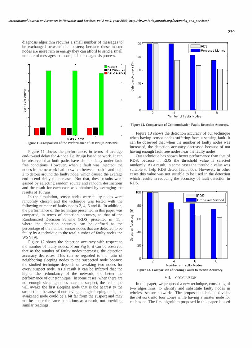
to diagnose faulty zone masters. On the other hand, the second algorithm is used to test and substitute faulty sensor nodes, i.e. non master nodes, in the network.
The simulation has shown that the proposed technique does not require a lot of messages to be exchanged in order to detect the fault master node. Also, it has shown that because the master nodes are connected in a De Bruijn graph, the end-to-end delay is low under faulty and fault free conditions. Furthermore, the simulation has shown the ability of the technique to identify several faulty nodes in the same zone. Also, it has illustrated that the technique is capable of identifying more than one faulty node in more than one zone at the same time. Finally the algorithm is tested by simulating two different scenarios. Our results show that the detection accuracy was very high when the number of faulty nodes was small compared to the number of sleeping node.
Future work for this work may include studying the effect of the second algorithm on the energy consumption and the life time of the network. In addition, the effect of having the sensor nodes in a zone connected in a De Bruijn graph will be studied.
REFERENCES [1] A.A.Taleb, D.K. Pradhan and T. Kocak, "A Technique to Identify and
Substitute Faulty Nodes in Wireless Sensor Networks," Third International Conference on Sensor Technologies and Applications, 2009. SENSORCOMM '09., pp.346-351, 18-23 June 2009.
[2] A. Mainwaring, Culler, D. Culler, J. Polastre, R. Szewczyk and J. Anderson , “Wireless Sensor Networks for Habitat Monitoring,” First ACM Workshop on Wireless Sensor Nerworks and Applications, Atlanta, Georgia, USA, Sept 2002.
[3] Y. Zou and K. Chakrabarty, “A Distributed Coverage and connectivity Centric Technique for Selecting Active Nodes in Wireless Sensor Networks,” on IEEE Trans. on Computers, vol. 54, no. 8, pp. 978-991, Aug 2005.
[4] K. Ssu, C. Chou, H. C. Jiau and W. Hu,“Detection and diagnosis of data inconsistency failures in wireless sensor networks,” in The Int. Journal of Computer and Telecommunications Networking, vol. 50,no. 9, pp. 1247-1260, June 2006.
[5] G. Gupta and M. Younis, "Fault-tolerant clustering of wireless sensor networks," IEEE Conf. on Wireless Communications and Networking, (WCNC). pp.1579-1584, March 2003
[6] Q. Liang, “Fault-tolerant and energy efficient wireless sensor networks: a cross-layer approach,” in Proceedings of IEEE Military Communications Conference (MILCOM ’05), vol. 3, pp. 1862–1868, Atlatnic City, NJ, USA, October 2005.
[7] A. Sheth, C. Hartung and R. Han (1999). A decentralized fault diagnosis system for wireless sensor networks. In: Proceedings of the 2nd IEEE International Conference on Mobile Ad-Hoc and Sensor Systems (MASS) 2005. pp. 192–194.
[8] I. Saleh, H. El-Sayed and M. Eltoweissy, "A Fault Tolerance Management Framework for Wireless Sensor Networks," Innovations in Information Technology, 2006 , vol., no., pp.1-5, Nov. 2006.
[9] J. Chen, S. Kher, and A. Somani “Distributed Fault Detection of Wireless Sensor Networks” . In Proc of the 2006 Workshop in Dependability issues in wireless ad hoc networks and sensor networks, L.A., California, USA, Sept. 2006.
[10] J. Staddon, D. Balfanz and G. Durfee, “Efficient tracing of failed nodes in sensor networks” . In Proc of the 1st ACM international workshop on Wireless sensor networks and applications, Atlanta, Georgia, USA, Sept 2002.
[11] B. Krishnamachari, S. Iyengar, "Distributed Bayesian algorithms for fault-tolerant event region detection in wireless sensor networks,"
Computers, IEEE Transactions on , vol.53, no.3, pp. 241-250, March 2004.
[12] Yue-Shan Chang; Tong-Ying Juang; Chih-Jen Lo; Ming-Tsung Hsu; Jiun-Hua Huang, "Fault Estimation and Fault Map Construction on Cluster-based Wireless Sensor Network," . IEEE International Conference on Sensor Networks, Ubiquitous, and Trustworthy Computing, 2006, vol.2, no., pp.14-19, 5-7 June 2006.
[13] T. Clouqueur, K.K. Saluja, P. Ramanathan, "Fault tolerance in collaborative sensor networks for target detection," Computers, IEEE Transactions on , vol.53, no.3, pp. 320-333, Mar 2004.
[14] Yongxuan Lai; Hong Chen, "Energy-Efficient Fault-Tolerant Mechanism for Clustered Wireless Sensor Networks," Proceedings of 16th International Conference on Computer Communications and Networks, 2007. ICCCN 2007., vol., no., pp.272-277, 13-16 Aug. 2007.
[15] Tsang-Yi Wang; Han, Y.S.; P.K. Varshney, Po-Ning Chen, "Distributed fault-tolerant classification in wireless sensor networks," IEEE Journal on Selected Areas in Communications, vol.23, no.4, pp. 724-734, April 2005.
[16] S. Hwang and Y. Baek, ”Fault Tolerant Time Synchronization for Wireless Sensor Networks,” LNCS-3894, Springer, pp. 480–493, March 2006.
[17] F. Koushanfar; M, Potkonjak; A, Sangiovanni-Vincentell, "Fault tolerance techniques for wireless ad hoc sensor networks," Sensors, 2002. Proceedings of IEEE , vol.2, no., pp. 1491-1496 vol.2, 2002.
[18] M. R. Samatham and D. k. Pradhan, “THE De Bruijn Multiprocessor Networ: A versatile Parallel Processing and Sorting Network for VLSI,” IEEE Trans. on Computers, Vol 38, No. 4, April 1989.
[19] D. K. Pradhan and N. H. Vaidya, “Roll-Forward Checkpointing Scheme: A Novel Fault-Tolerant Architecture,” on IEEE Trans. On Computers, vol. 43, no. 10, pp. 1163-1174, Oct. 1994.
[20] D. K. Pradhan, and S. M Reddy, “A fault-tolerant communication architecture for distributed systems,” IEEE Trans. on computers., pp. 863-870, 1982.
[21] M. Andersson, D. Henriksson, A. Cervin and K. Årzén, “Simulation of wireless networked control systems” . In Proc of the 44th IEEE conference on Decision and control and European Control onference ECC, Seville, Spain 2005.
[22] TrueTime, Lund University. (2008, June 10) [Online]. Available: http:// www.control.lth.se/truetime/
240
International Journal on Advances in Networks and Services, vol 2 no 4, year 2009, http://www.iariajournals.org/networks_and_services/
Integrated System for Malicious Node Discovery and
Self-destruction in Wireless Sensor Networks
Madalin Plastoi
Politehnica University of TimisoaraTimisoara, Romania
Constantin Volosencu
Politehnica University of TimisoaraTimisoara, Romania
Ovidiu Banias
Politehnica University of TimisoaraTimisoara, Romania
Roxana Tudoroiu
Politehnica University of TimisoaraTimisoara, Romania
Daniel-Ioan Curiac
Politehnica University of TimisoaraTimisoara, Romania
Alexa Doboli
State University of New YorkStony Broke, New York, USA
Abstract — With the tremendous advances of the wirelessdevices technology, securing wireless sensor networks becamemore and more a vital but also a challenging task. In this paperwe propose an integrated strategy that is meant to discovermalicious nodes within a sensor network and to expel themfrom the network using a node self-destruction procedure.Basically, we will compare every sensor reading with itsestimated values provided by two predictors: an autoregressivepredictor [1] that uses past values provided by the sensorunder investigation and a neural predictor that uses pastvalues provided by adjacent nodes. In case the absolutedifference between the measured and the estimated values aregreater then a chosen threshold, the sensor node becomessuspicious and a decision block is activated. If this blockdecides that the node is malicious, a self-destruction procedurewill be started.
Keywords - wireless sensor networks, prediction, maliciousnode discovery, self-destruction
I. INTRODUCTION
With the continuous progress in micro-electro-mechanical systems (MEMS) and radio technologies, a newconcept arose - wireless sensor networks (WSN). A wirelesssensor network, being a collection of tiny sensor nodes withlimited resources (limited coverage, low power, smallermemory size and low bandwidth), proves to be a viablesolution to many challenging civil and military applications.Their deployment, sometimes in hostile environments, canbe dangerously perturbed by any type of sensor failure or,more harmful, by malicious attacks from an opponent.
Sensor networks because of their specific limitations aresusceptible to various kinds of attacks that cannot beprevented only by traditional methods (e.g. cryptography):eavesdropping, traffic analysis, selective forwarding,
spoofing, wormhole attack, sinkhole attack, Sybil attack andHello flood attack are the most significant [2]. But, almostcertainly the most important danger, due to the inherentunattended characteristic of wireless sensor networks, isrepresented by node-capturing attack [3], where an enemyacquires full control over sensor nodes through directphysical contact. A node capturing attack is very feasiblebecause of at least two reasons: a) practically, we cannotdemand an efficient access control to thousands of nodesdistributed in a large territory; and b) it is very difficult toassure tamper-resistance requirements because sensor nodesfrequently need to be inexpensive to justify their use.
After an attacker gains the physical control over a sensornode he can extract secret information such as cryptographickeys to achieve unrestricted entrance to higher networklevels, or by using reverse engineering techniques he canfind security holes to compromise the entire sensor network.
Our proposed countermeasure is based on the fact that acorrupted node is better to be expelled from the network assoon as its malicious activity is started [4]. Even if moresensors are expelled, the WSN will function as designedbecause of one inherent feature: spatial redundancy [5].
In order to identify a corrupted sensor node, wepresumed that even if it may still send authenticatedmessages (e.g., it can use the cryptographic keys alreadystored in its memory), it might not operate according to itsoriginal specifications sending incorrect readings to the basestation. We will identify these sensors by using predictiontechniques and will eliminate them by starting a self-destruction node procedure.
The rest of the paper is organized as follows. The secondsection presents a detailed description of our strategy.Section 3 presents the technique used for the self-destructionprocedure applied to corrupted nodes. In the last twosections, experimental results and conclusions are offered.
241
International Journal on Advances in Networks and Services, vol 2 no 4, year 2009, http://www.iariajournals.org/networks_and_services/

II. PREDICTION BASED METHODOLOGY
In a large number of applications where wireless sensornetworks interact with sensitive information or function inhostile unattended environments, it is crucial to developsecurity related mechanisms.
Due to their nature, these networks have to resist to aplethora of possible attacks. The attackers will try to obtainin-network information or to corrupt the network partially ortotally. For making this possible, the attackers will try to gaincontrol over one or several network nodes. Our proposeddefending strategy is based on the detection of malicioussensor nodes using predictors and the elimination of theireffects by expelling them from the network using a self-destruction node technique.
A. The Sensor Network Assumptions
In order to assure a high rank of efficiency for ourmalicious node detection and self-destruction strategy wechose a sensor network having the following features:
a) The sensor network is static, i.e., sensor nodes arenot mobile; Moreover, each sensor node knows its ownposition in the field.
b) The base station, sometimes named access point,acting as a controller and as a key server, is supposed to be alaptop class device and supplied with long-term power. Wealso assume that the base station will not be compromised.
c) Between the three most common wirelesstopologies (star, mesh and cluster-tree) we chose a startopology (e.g. Cellular Wireless Network [6] and SENMA[7]) for our sensor network. Star topology is a point-to-pointarchitecture where each sensor node communicates directly
with the base station. The main characteristics of the startopology are: there are no node-to-node connections and nomulti-hop data transmission; sensor synchronism isunnecessary; sensor do not listen, only transmit and onlywhen polled for; complex protocols are avoided;dependability of individual sensors is much less significant.Because of these features, attacks on routing protocols(spoofing, selective forwarding, sinkhole attack, wormholeattack, Sybil attack and Hello flood attack) are almostimpossible.
d) We rely on efficient secret-key cryptography withpre-distributed keys using Skipjack, RC5 or AES algorithmsto encipher all data communications inside the sensornetwork; These three symmetric encryption algorithms havea common attribute that makes them an attractive alternativein case of sensor networks: they are able to encrypt short ormedium size messages, like the ones send by sensors andreceived by base stations, in the case of limited powerconsumption. By using such appropriate cryptographictechniques the damaging potential of the passive attacks(eavesdropping and traffic analysis) can be ignored.
e) The measurements supplied by each sensor have animportant deterministic character, rather than a strictlyrandom (stochastic) one. In this case there exists acorrelation between past values and the current one, givingus the power of prediction. As an example, the future valuesof temperature measurements in a location are stronglyrelated with past and present values, so a prediction methodcan be applied.
Figure 1. Malicious node discovery and self-destruction with mixed prediction
B. The Proposed Strategy
Our strategy exploits two types of observations over thecurrent and past measurements of the wireless sensor
network nodes. First, the temporal redundancy in the sensethat previous provided measurements from each sensor willbe used to decide if the given sensor operates as desired ornot. And second, based on the past and present values of
242
International Journal on Advances in Networks and Services, vol 2 no 4, year 2009, http://www.iariajournals.org/networks_and_services/
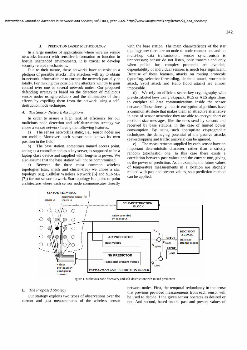
neighboring nodes, the operation of the given sensor isclassified as right or wrong.
We decided to use a mixed estimation and predictionsystem with two predictors – an autoregressive predictor(AR) and a neural network predictor (NN). The firstpredictor will describe the node evolution using its pastvalues while the second one will describe node evolutionusing present and past values provided by neighboringnodes.
In Fig. 1 is presented the system architecture, composedof 4 major components: a) The Wireless Sensor Networkunder investigation; b) The Estimation and PredictionBlock; c) The Decision Block; and d) The Self-destructionProcedure. The Estimation and Prediction Block includestwo on-line predictors, one autoregressive predictor and oneneural network predictor. The outputs of these twopredictors represent the inputs for the Decision Block. Atthis level the system will provide automatic decisions uponengaging or not the self-destruction procedure for the givennode.
In the following paragraphs we will present bothpredictors, including the mixed strategy.
Our stratagem to identify a corrupted sensor node isbased on the fact that even if it may still send authenticateddata it may not operate according to initial requirements,sending incorrect readings to the base station. These nodeswill be identified in the moment they begin to broadcasterroneous information. For this purpose, we will presentfurther two types of predictors, one autoregressive predictor,and one neural network predictor. Based on these predictorswe will decide if a self-destruction procedure is needed.
In order to implement the first predictor, we consideredthat an autoregressive (AR) model efficiently approximatesthe evolution in time of the measurements provided by eachsensor. An autoregressive or AR model describes theevolution of a variable only using its past values. This classof systems evolves due to its "memory", generating internaldynamics, and is defined as follows:
)()(...)1(1)( tntxnatxatx , (1)
where )(tx is the measurement series under investigation,
ia are the autoregression coefficients, n is the order of the
autoregression and is assumed to be the Gaussian white
noise. By convention, the time series )(tx is assumed to be
zero mean. If not, another term 0a is added in the right
member of equation (4). Establishing the correct model oforder n is not a simple task and is influenced by the type ofdata measurements and by computing limitations of the basestation. Reasonable values of the order n are between 3 and6.
If the ia coefficients are time-varying, the equation (1)
can be rewritten as:
)()()(...)1()(1)( tntxtnatxtatx . (2)
The model (2) can be used either to estimate the coefficients
)(tai in case the time series )(),...,( ntxtx are known
(recursive parameter estimation), either to predict future
value in case that )(tai coefficients and past values
)(),...,1( ntxtx are known (AR prediction).
In parallel with the AR predictor, we use a three orderfeed forward neural network predictor with two hiddenlayers. The input layer consists of neurons which areassociated with values provided by adjacent nodes atmoments t, t-1 and t-2. The output layer has only oneneuron for the estimated value.
For network’s node A, the estimated value by the neuralpredictor is:
)),(),...,1(()()(ˆ )(,, NNAadjAadjA BntXtXftNNAx , (3)
TadjmAadjAadjA itxitxitX ,1,, ,...,)( , (4)
TadjmAadjANNA bbB ,1,)( ,..., , (5)
where: itx adjkA , is the value from the adjacent node k at
it moment, )(NNAB is a vector containing the trust
factors of each of the m adjacent nodes of A, and n is thepredictor order.
The trust factor )(NNAb has a linear dependence on the
previous node trust factor and the error value. However, the
computation of )(NNAb is made in the decisional block.
After the node’s output of the neural prediction, an errorvalue is obtained:
)(ˆ)()( )()( txtxte NNAANNA . (6)
C. The Autoregresive Prediction
Our strategy exploits the temporal redundancy in thesense that previous provided measurements from eachsensor will be used to decide if the sensor operates asdesired or not. The plan is the following: an attacked sensornode that will attempt to insert false information into thesensor network will be recognized by comparing its outputvalue with the value predicted using past readings offeredby that specific sensor (Fig. 2). In the case that anymalicious activity is observed, the Decision Block istriggered to decide if the self-destruction procedure must bestarted for this specific node in order to prevent its furtherundesired activity.
The complete mechanism workflow runs while networkis active. By considering a specific node symbolized by A,this process is done in the following steps:
243
International Journal on Advances in Networks and Services, vol 2 no 4, year 2009, http://www.iariajournals.org/networks_and_services/
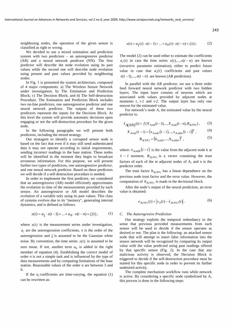
Figure 2. Autoregressive predictor
a) Associate a node trust indicator with every sensornode. The specified sensor node A will have a trust factor
denoted by )( ARAb . This integer value is initially set to zero
( 0)( ARAb for a fully reliable sensor node) and is
incremented during our methodology every time a potentialmalicious activity is encountered. This trust factor must bereset to zero, if no potential malicious activity isencountered for a long period of time. The node trustindicator represents, in other words, the perception ofconfidence between the WSN and that specific sensor.
b) At every moment of time t, estimate the present value
)()(ˆ tARAx provided by sensor node A, using the past readings
)()( itx ARA provided by the same sensor A. For the
sensor A, we can write:
))()(),...,1()(()()(ˆ ntARAxtARAxftARAx (7)
where n is the estimator’s order. In our approach, an on-lineAR predictor performs this step.
c) Compare the present value )(txA measured by the
sensor node A with its estimated value )()(ˆ tARAx by
calculating the error:
)()(ˆ)()()( tARAxtAxtARAe (8)
d) Increment the node trust indicator Ab if the error
)()( te ARA exceeds a given threshold AR : ARtARAe )(
(this is done only one time inside a transitory time zone –due to the internal structure of recursive predictors, an errorobtained at instant time t, is propagated/attenuated in therecursive predictor response for some instants, obtaining atransitory regime). If the node trust indicator is higher than achosen value )(ARAb , the node could be declared as
potentially malicious and depending on the Decision Blockoutput, a self-destruction procedure could be started for theA node.
The associated pseudocode is presented in Fig. 3.
//this function is performed for each node in the networkint Autoregression(int nodeId){
SET )(ARAb , )(ARA ; //node trust indicator, threshold
WHILE (network is active){…
Ax =READ sensor A; //get sensor actual value for node ID equal
//with nodeID…
)(ˆ ARAx = ARpredict(prior Ax values); //call AR prediction
)( ARAe =)(ˆ ARAxAx ; //calculate the error
IF (ABS ( )( ARAe ) > )( ARA )
{IF (AR predictor is not in transitory regime)
{ )(ARAb = )(ARAb + 1; //increment node trust indicator
START thread TRANSITORY_REGIME;//a counter set on k //and will be decremented every//instant until it becomes zero
}DECISION_BLOCK (node with node ID equal to nodeID);
//call //decision method}}…}
Figure 3. AR implementation pseudocode
First of all, we have to associate a threshold 0AR for
every sensor node. This threshold will be used to decide if asensor operates normal or abnormal and its measured valuedepends on the type of the sensor and its specific anddesired operation in real environment. For a specific sensor
A, the threshold will be denoted by )( ARA .
After this initialization, at every instant t, we willcompute the estimated value )()(ˆ tARAx relying only on
past the values )0(),...,1( AA xtx and we will use both
parameter estimation and prediction as presented in thefollowing steps:
First step: we will estimate the parameters )(tai using a
recursive parameter estimation method. From a largenumber of methods for estimating AR coefficients wedecided to use a numerically robust RLS (recursive leastsquare) variant based on orthogonal triangularization,known in literature as QRD-RLS [8]. One of the reasons isthat it can be implemented efficiently on the base stationslevel (laptop class device).
Second step: we will obtain the prediction
value )(ˆ)( tx ARA using the following equation:
)()()(...)1()(1)()(ˆ tntAxtnatAxtatARAx (9)
244
International Journal on Advances in Networks and Services, vol 2 no 4, year 2009, http://www.iariajournals.org/networks_and_services/
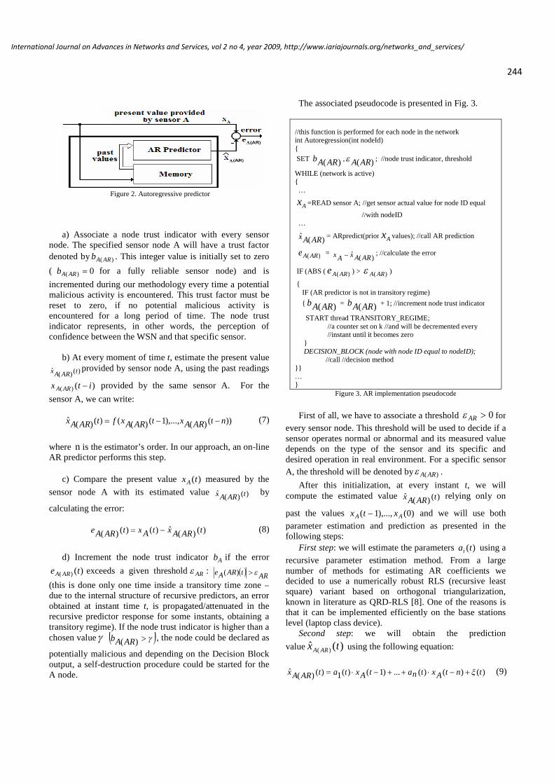
The corresponding pseudocode for implementing theestimation procedure is presented in Fig. 4:
float ARpredict(prior Ax values)
{ CALCULATE autoregression coefficients ai ;// an estimation using QRD-RLS method
CALCULATE predicted value )(ˆ ARAx ;
//compute sensor predicted value as a result of (9)
RETURN )(ˆ ARAx ; }
Figure 4. Autoregressive prediction pseudocode
Following, we will compare the present value
)t(x A measured by the sensor node with its estimated
value )()(ˆ tARAx , and the error )( ARAe will be computed
using equation (8).
D. The neural network prediction
In order to improve the efficiency and reliability of theEstimation and Prediction Block, we implemented a neuralnetwork predictor based on measurements provided bycontiguous sensors [9]. This predictor will work in parallelwith the autoregressive predictor to discover all maliciousactivity. In Fig. 5 the neural network predictor is presented:
Figure 5. Neural Network predictor
A neural network predictor consists of three or morelayers of artificial neurons (Fig. 6). Usually, neural networkshave at least three layers, an input layer, an output layer anda hidden one. Our implemented neural network has fourlayers because we used two hidden layers. Neurons arelinked one with each other through quantitative relationsknown as weights. Each layer is activated by an activationfunction. Most used activation functions are: direct identity(for input layers), sigmoid, hyperbolic tangent and linearfunctions. In fact this neural predictor model exposes acomposition function which describes how the inputs aretransformed into outputs.
Figure 6. Neural network predictor
Each neuron implements the following function:
i
ii xgKxf ))(()( , (10)
where K is a composition function, i are the weights, and
ig is a vector containing neuron’s inputs
),...,,( 21 ngggg [10].
In order to use a neural network predictor, two stepsmust be performed:
Neural network training - will be established the number
of hidden neurons and the neural network weights i by
performing successive training sessions using Levenberg-Marquardt method [11]. For the hidden layers we will usehyperbolic tangent activation function and for the outputlayer we will use a linear activation function. This trainingstep is done off-line, prior to the neural network predictorimplementation on the base station.
Neural network on-line prediction - will be obtained the
prediction value )(ˆ)( tx NNA , computing for each neuron the
equation (10). This procedure starts with the neurons fromthe input layer and ends with the neuron from the outputlayer and it’s implemented as an on-line predictor on the
base station. In the end, the error )( NNAe is computed using
equation (6). The associated pseudocode for the neuralnetwork predictor is presented in Fig. 7:
//this function is performed for each node in the networkint NNPrediction(int nodeId){
SET )(NNAb , )(NNA ; //node trust indicator, threshold
WHILE (network is active){…
Ax =READ sensor A; //get sensor actual value for node ID equal
//with nodeID…
245
International Journal on Advances in Networks and Services, vol 2 no 4, year 2009, http://www.iariajournals.org/networks_and_services/
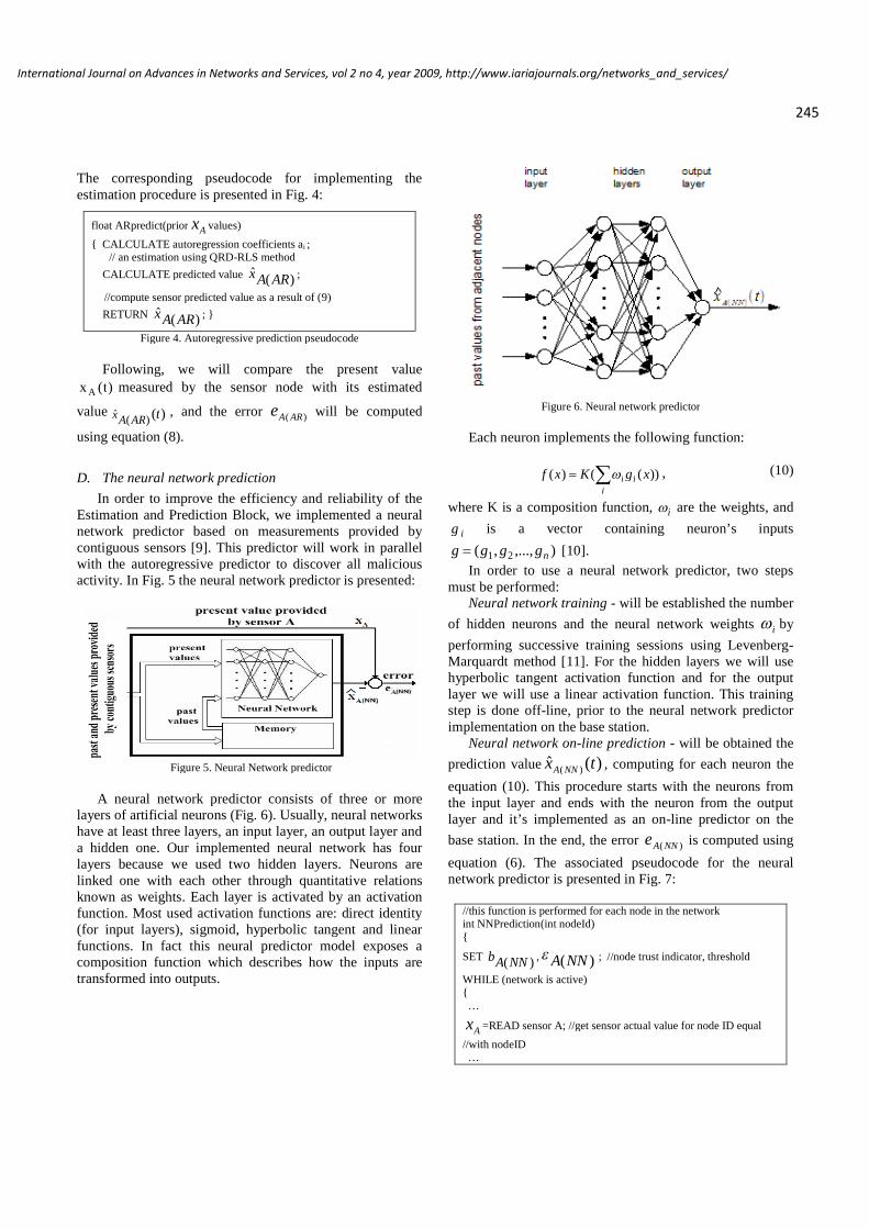
)(ˆ NNAx = NNpredict (present and past adjacent nodes values);
//call NN prediction
)( NNAe = )(ˆ NNAxAx ; //calculate NN error
IF (ABS ( )( NNAe ) > )( NNA )
IF (NN predictor is not in transitory regime)
{ 1)()( NNAbNNAb //increment node trust indicator
START thread TRANSITORY_REGIME;//a counter set on k //and will be decremented every//instant until it becomes zero
}DECISION_BLOCK (node with node ID equal to nodeID);
//call decision method; Fig. 8.}…}
Figure 7. NN implementation pseudocode
The initialization steps are the same as for the AR
prediction, a threshold 0)( NNA being associated with
sensor node A.At every instant t, we will compute the estimated value
)(ˆ)( tx NNA relying on the present and past values of the
adjacent neighbors of the node A.
E. The Decision Block
The Decision Block will provide the decision to start theself-destruction procedure of a malicious node, based on the
pair of errors, ( )()( tARAe , )()( tNNAe ) that will be used as
inputs in an expert system, by computing two trust
indicators )( ARAb and )( NNAb .
These trust indicators are initially set to zero
)0,0( )()( NNAARA bb signifying that in the beginning,
the sensor is considered to be fully reliable. After that, whenpotential malicious activity is detected, the trust indicatorsare incremented. In order to filter possible sporadicmalfunctions of the sensors, these counters must be reset tozero at specific intervals in time.
An efficient Decision Block can be implemented eitheras a fuzzy-based system, either as a rule-based system. Inthis paper we have chosen a rule-based approach. TheDecision Block architecture is presented in the Fig. 8:
Figure 8. Decision Block
Based on the previously defined patterns & scenarios,the decision block was implemented as an expert system.We defined two parameters , , with 0 , for
classifying each of the trust factors )()( , NNAARA bb , as
follows:
a) 5 categories for )( ARAb
)()(
)()()(
);,(
;);,0(;0
ARAARA
ARAARAARA
bb
bbb (11)
b) 5 categories for )( NNAb
)()(
)()()(
);,(
;);,0(;0
NNANNA
NNANNANNA
bb
bbb (12)
Using this classification, we developed 25 types of rules for
the pair ),( )()( NNAARA bb having the inputs )( ARAb , )(NNAb ,
, , and the outputs the activation or not of self-
destruction procedure. The rules formalization is presentedin Fig. 9:
RULE X: // activation of self-destruction procedure
if Evaluate( )( ARAb , )( NNAb , , ) then
Self_Destruction( sensor A);
RULE Y: // not activation of self-destruction procedure
if Evaluate( )( ARAb , )( NNAb , , ) then
DoNothing();Figure 9. Rule definition
As presented in Fig. 9, the activation of certain rules lead tothe self-destruction procedure of the given node(Self_Destruction procedure). This procedure is presented inthe following paragraph.
246
International Journal on Advances in Networks and Services, vol 2 no 4, year 2009, http://www.iariajournals.org/networks_and_services/
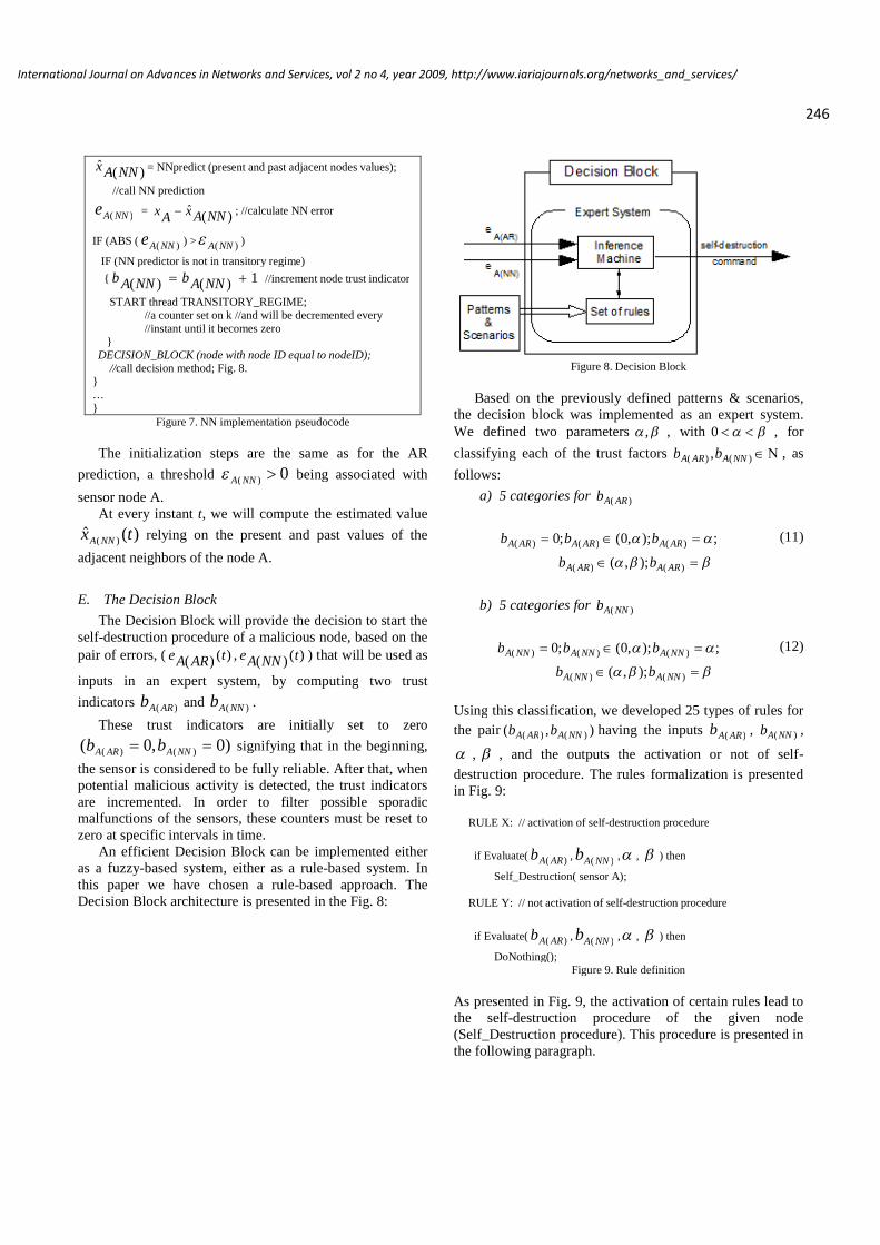
III. MALICIOUS NODE SELF-DESTRUCTION
If a certain node has been tagged as malicious, the basestation will initiate a self-destruction sequence for thatspecific node. The self-destruction routine is divided intoseveral actions: Erase node RAM memory that contains susceptible
network information, driven software and cryptographickeys and also other additional memories (e.g. flashmemory, if present);
Drain node battery in different ways like R/T radio floodor node logical unit infinite cycle [12];
Destroy node radio device; Delete node unique identifier from the lists of each of
the neighbor nodes, including base station; This way analready captured node won’t gain authentication rights ifan attacker tries to reintroduce it in the network (willdisable auto-organization property);
Mask node measurement nature by hiding the type of thesensor that has been used (each node has one or moresensors and knows in a logical way which of them isused for measurements).
The above actions have to be performed in order of theirimportance, although some kind of concurrency could beassured. For example: the initiation of self-destruction couldstart the procedure for draining node battery, but in the sametime it could conduct erasing actions for memory andcryptographic keys.
Self-destruction should take into consideration allnetwork characteristics from design to deploymentincluding the topology. Also it strongly depends on the nodehardware profile. For the proposed star network model, self-destruction will imply only the base station and thecompromised node – as we stated earlier, each nodecommunicates directly with the base station.
Basically, self-destructive sequence may be a softwareroutine embedded into node’s memory or sent bit by bitfrom the base station to the aimed node. Entire code has tobe compatible with nodes and base station operating system.The pseudocode for node self-destruction is presented inFig. 10:
void Self_Destruction (sensor A)WHILE (sensor A is in network){START threadCONSUME battery energy //broadcast specific messages;
START thread{ERASE node memory; //erase RAM and flash memory
DISABLE auto-organization property;//delete node identifier from all neighbor’s lists
DESTROY node radio device;MASK node measurement nature;
//for hiding the type of the sensor}}
Figure 10. Node self-destruction pseudocode
In the optimistic scenario, after self-destructive routinewas initiated, the intended node is destroyed and obvious,undetectable in the network. All references to its identifierwill disappear from all network devices. Cryptographic keysand stored information will be also deleted.
In the pessimistic scenario, the self-destructive responsewon’t have any triggered action attached to it; the corruptednode will still be alive in a fully or partially functional state.This scenario will have to be avoided by reducing theprobability of some unfortunately events like:1. Self-destructive routine was not suitable implemented
for node hardware profile;2. The node’s software is modified by the enemy in such
way that it doesn’t accept incoming messages from thebase station, it only sends malicious data;
3. Node battery is almost exhausted at the moment ofexecuting the routine. In this case no memory erasingwill be performed. The attacker will replace the batteriesand the node will be partially or totally running.
Our solutions for avoiding these incidents are: testing ofthe self-destruction code on every type of sensor nodes thatis included in the WSN; hiding the self-destruction routineinto the node’s memory; paying attention to the energyconsumption on each sensor.
IV. CASE STUDY
For validating our strategy, we used a Crossbow wirelesssensor networks, containing 15 Mica2 nodes and one basestation in a star topology. The sensors were set to measurethe temperature in a room. In order to model an attack uponsensor A, we made the following experiments: First case study: at specific moments in time we
intervened with an electric incandescent lamp (200watts) placed very near to sensor A, for disrupting thenormal functioning of only one specific node;
Second case study: at specific moments in time weplaced a heat source near to the network. In this case,normal functioning was disrupted for several networknodes, including the sensor node A.
We set up both predictors with the order 3n , the
thresholds CARA1)( , CNNA
2)( and the pair
),( = (3, 5).
We considered that the node A has 8 adjacent neighbors.Past and present values from these adjacent neighbors willbe used for neural network prediction of the node A value ata certain moment in time, while past values of node A willbe used for autoregressive prediction.
The predictor contains 4 layers: one for input with 24neurons, two hidden layers and one output layer for theestimated value. The hidden layers have 48 and 24 neurons.
The neural network predictor was trained using threearrays of inputs corresponding to the 8 adjacent neighbors at
247
International Journal on Advances in Networks and Services, vol 2 no 4, year 2009, http://www.iariajournals.org/networks_and_services/
three moments of time (predictor order) and a target valuefor node A (Fig. 11). The training was performed offline,using the Matlab toolbox functions and features (e.g. trainfunction, nntool UI) [13].
Figure 11. Neural network training session
After the training step was finished, the neural networkpredictor was installed on the base station node.
A. First case study
In this case study, we simulated an attack over a certainnode, by inserting a heated lamp in its close neighborhood,leaving the other nodes unaffected (Fig. 12). We observedthe result of both predictors and the system’s decisionmaking.
Figure 12. First case study description
In Fig. 13a we presented the sensor’s A output timeseries, including our three “malicious” interventions atinstants t=15sec, t=20 sec and t=27 sec. In Fig. 13b and 13cwe presented the time variation of the AR and NN predictedtime series, and in Fig. 13d and 13e we presented the
evolution in time of the errors tARAe )( and tNNAe )( .
As node A is the only attacked node, the NN predictorestimated value remains in the limits of the adjacent nodesreal values, while the AR predictor estimated value is in thevicinity of the attacked node real values,
)()( )()( tete ARANNA , }27,20,15{t . From the graphics
depicted in the Fig. 13d and 13e, we can observe that the
trust factors )( ARAb and )(NNAb have the same value,
3)()( NNAARA bb . The decision to engage the self-
destruction procedure is made based on a predefined rule:
If ( )( NNAb == AND )( ARAb == )
Self_Destruction(sensor A);
The results are as expected: after exceeding the
thresholds )(,)( NNAARA for three times for both
predictors (Fig. 13d, Fig. 13e), the sensor A is expelled fromthe WSN by starting its self-destruction procedure. Thisresult can be observed in Figure 13 where no more readingsare obtained from sensor A after t=27 sec.
a)
b)
c)
248
International Journal on Advances in Networks and Services, vol 2 no 4, year 2009, http://www.iariajournals.org/networks_and_services/
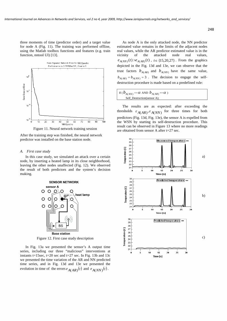
d)
e)
Figure 13. a)The sensor’s output time series;b)AR Predicted time series; c) NN Predicted time series;d) AR Prediction error time series; and e) NN Prediction
error time series;
B. Second case study
In this case study, a heat source is activated at timemoments t=15sec, t=20 sec, and t=27 sec in order to affectall sensor nodes, which represent a normal operatingscenario - it is not a simulation of an attack. All networknodes are affected by a hot air wave.
Figure 14. Second case study description
The evolution in time of the AR predicted values and theevolution of the error tARAe )( are similar to the previous
case study.Assuming that node A has 8 adjacent neighbors, since
all these neighbors are also affected by this heat wave (Fig.14), the neural network predicted time series for the node Awill have a similar evolution with the AR predictor timeseries (Fig. 15b, Fig. 15c). The computed error for the NNpredictor case is lower than the computed error for the AR
predictor case, ),()( )()( tete ARANNA }27,20,15{t . Also
the error )()( te NNA is lower than the threshold CA2 .
The decision to engage or not the self-destruction procedureis made based on a predefined rule:
if ( )( NNAb == 0 AND )( ARAb == )
DoNothing();
By activating this rule, the Decision Block decided that noattack was performed over the node A.
a)
b)
c)
d)
249
International Journal on Advances in Networks and Services, vol 2 no 4, year 2009, http://www.iariajournals.org/networks_and_services/

e)
Figure 15. a)The sensor’s output time series;b)AR Predicted time series; c) NN Predicted time series;d) AR Prediction error time series; and e) NN Prediction
error time series;
Due to the diversity of the attack patterns we proved thatthe use of the two predictors in parallel is more accuratethan the usage of a single predictor. For example, the use ofonly one predictor (AR predictor) in the second case studycan lead to a wrong result – the self destruction of a normal-functioning node.
V. CONCLUSIONS
Security issues related to WSN become more and morean important research area. Detecting abnormal/maliciousoperation of motes and offering efficient countermeasuresrepresents a difficult task. In this paper we propose acombined strategy that not only detects the corrupted nodes,but also excludes their malicious activity using a self-destruction node technique. Due to the inherent spatialredundancy feature of WSN, applying a self-destructionprocedure to the corrupted nodes has no majorinconveniences, extending the secure operation of the entiresensor network.
The integrated system presented in this paper has somenoticeable advantages: decision for node self-destruction istaken based on two predictions, two errors and two trustfactors, therefore the accuracy is better; the whole systemtakes into consideration not only the evolution of a specificnode, but also its neighbors evolution; as the two predictormodels have a different nature, different attack patternscould be treated. Our strategy has also a drawback: a biggercomputational power is needed at the base station level.
ACKNOWLEDGMENT
This work was developed in the frame of PNII-IDEI-PCE-ID923-2009 CNCSIS - UEFISCSU grant and waspartially supported by the strategic grant POSDRU
6/1.5/S/13-2008 of the Ministry of Labor, Family and SocialProtection, Romania, co-financed by the European SocialFund – Investing in People.
REFERENCES
[1] D. Curiac, M. Plastoi, O. Banias, C. Volosencu, R. Tudoroiu,A. Doboli, “Combined Malicious Node Discovery and Self-Destruction Technique for Wireless Sensor Networks”, ThirdInternational Conference on Sensor Technologies andApplications, Athens, Greece, June 18-23, pp. 436-441.[2] Karlof C., Wagner D., “Secure routing in wireless sensornetworks: attacks and countermeasures”, Proceedings of the 1stIEEE International Workshop SNPA2003, Anchorage, USA, May2003, pp. 113-127.[3] Becher A., Benenson Z., Dornseif M., “Tampering with motes:Real-world physical attacks on wireless sensor networks”Proceedings of the 3rd International Conference on Security inPervasive Computing (SPC), York, UK, April 2006, pp.104-118.[4] D.I. Curiac, O. Banias, F. Dragan, C. Volosencu, O. Dranga,“Malicious Node Detection in Wireless Sensor Networks Using anAutoregression Technique”, ICNS2007, Athens,Greece, June2007.[5] Y. Gao, K. Wu, and Fulu Li, “Analysis on the Redundancy ofWireless Sensor Networks,” ACM WSNA’03, San Diego, USA,September 2003, pp.108-114.[6] J. Feng, F. Koushanfar and M. Potkonjak, “System-Architectures for Sensor Networks Issues, Alternatives, andDirections”, Proc. ICCD’02, Freiburg, Germany, Sept. 2002,pp.226-231.[7] L. Tong, Q. Zhao and S. Adireddy, “Sensor Networks withMobile Agents", Proceedings IEEE 2003 MILCOM, Boston, USA,October 2003, pp.688-694.[8] B. Haller, J. Gotze and J. Cavallaro, “Efficient Implementationof Rotation Operations for High Performance QRD-RLSFiltering”, ASAP '97 Proc., 14-16 July 1997, Zurich, Switzerland,pp. 162-174.[9] D.I. Curiac, C. Volosencu, A. Doboli, O. Dranga and T.Bednarz, “Discovery of Malicious Nodes in Wireless SensorNetworks using Neural Predictors”, WSEAS Transactions onComputer Research, Issue 1, Volume 2, January 2007, pp. 38-43.[10] B. D. Ripley, “Pattern Recognition and Neural Networks”,Cambridge: Cambridge University Press, 1996, pp. 143-162.[11] J. More “The levenberg-marquardt algorithm, implementationand theory”, In G. A. Watson, editor, Numerical Analysis, LectureNotes in Mathematics 630, Springer-Verlag, 1977.[12] A. A. Pirzada and C. McDonald: “Kerberos assistedAuthentication in Mobile Ad-hoc Networks”, Proceedings of the27th Australasia.[13] Howard Demuth,Mark Beale,Martin Hagan “Neural NetworkToolbox™ 6 User’s Guide”, March 2008, pp. 2-71.
250
International Journal on Advances in Networks and Services, vol 2 no 4, year 2009, http://www.iariajournals.org/networks_and_services/

A Novel Approach to Indoor Location SystemsUsing Propagation Models in WSNs
Gomes GonçaloInstituto Superior Técnico
Inesc-IDLisbon, Portugal
Email: [email protected]
Sarmento HelenaInstituto Superior Técnico
Inesc-IDLisbon, Portugal
Email: [email protected]
Abstract— This paper describes a location system for personsand objects in an indoor environment, where wireless nodes caninclude sensors and provide unique identifiers. The system nodes,using ZigBee technology, can function as RFID tags, havingeach one a unique EPC identification number. Sensors can beassociated with the wireless nodes Zigbee to create applicationsfor home, health and traffic control.
Existemt location systems are analyzed, with emphasis onindoor location systems.The implemented location algorithmincludes a propagation model based on the wall attenuation factortogether with triangulation.
A variety of tests were carried out in an indoor environment.Results demonstrate that the location system is viable, showingitself to be effective, flexible and easily adaptable to variouslocations.
Keywords - Location, Propagation, Triangulation, WAF, ZigBee,Wireless.
I. INTRODUCTION
History shows that progress and technological developmentare inevitable, actually becoming a need in the globalise worldof nowadays. Telecommunications are currently essential inworld economy operations of any modern society, being,wireless network systems one of the greatest developmentsin the area of communications. An example of such a net-work, is a WSN (Wireless Sensor network), where spatiallydistributed autonomous devices, equipped with sensors, areused in environment monitoring, traffic control, healthcare,home automation, etc. RFID (Radio Frequency Identification)is also a wireless technology. The development of RFID,besides the advantages in several areas, has also been a startingpoint to technological evolution in location systems. Therehas been a rising interest in location techniques that hasbeen motivating allot of research in this area. In locationsystems there are two types of scenarios: outdoor locationand indoor location. Each one of these scenarios presentsitself with different characteristics and challenges, being thatindoor location systems are the hardest to implement given itscomplexity and all the factors that have to be considered. RFIDand WSN can be used together. Furthermore, generations ofRFID tags include sensors, and WSNs that require automaticidentification mechanisms [1].
Lately, there has been a growing interest in the integrationof RFID and WSN (Wireless Sensor Network) systems. These
technologies can originate the development of a variety ofapplications, particularly in terms of location, in residentialenvironments, corporate environments and critical infrastruc-tures worldwide [1]. ZigBee is a wireless technology that iswell suited for WSN. Besides, it can be used to build activeRFID tags. The use of RFID technology with ZigBee protocolprovides the study of effective, low energy consumption, andfinancially accessible location systems. In this paper we willexplore the use of Zigbee in order to build an indoor locationsystem. Based in this system that locates objects in indoorenvironments, objects can be identified and sensing variablescan be measured.
It’s precisely the fusion of RFID with WSN that is thestarting point of this work. The goal is make use of the RFIDcapabilities in automatic identification of people and objects,based on a ZigBee network, to develop an indoor locationsystem. In order to develop a location system it’s necessary tostudy the existing location methods and algorithms, especiallythose that focus in indoor location. It’s important to maximizethe advantages offered by the use of RFID and ZigBeetogether. Knowing that the goal is to achieve a system thatis both easily adaptable to various location environments andflexible, it’s necessary to give more attention to the locationmethods that use electromagnetic waves propagation models.
A starting point to the development of an indoor locationsystem is the definition of the location method. In this paper,we propose a location system that uses triangulation togetherwith a propagation model. The main obstacles in using trian-gulation are: the selection of three network devices and theestimation of the distance between fixed and mobile devices.The goal in the selection of the three network devices is to havethem as closest as possible to the mobile device improvingthe accuracy of the system. In order to estimate the distancebetween fixed and mobile devices, RSSI (Received SignalStrength Indicator) measures are made so that the distancecan be estimated through the use of a propagation model. Theuse of RSSI leads to a certain degree of inaccuracy due tomultipath effect, mainly caused by the indoor environment ofa building as well as the distance between a transmitter and areceiver.
The paper is organized as follows. After this introduction,
251
International Journal on Advances in Networks and Services, vol 2 no 4, year 2009, http://www.iariajournals.org/networks_and_services/
section 2 presents the state of the art concerning locationsystems, emphasizing indoor location. The indoor propagationmodels are described in section 3. Section 4 presents thedeveloped system. In section 5, the system characterizationis presented, being the results discussed in section 6. Section7 presents some conclusions.
II. LOCATION SYSTEMS
The success of the GPS system for monitoring and locatingobjects in outdoor environments, encouraged the application ofsimilar techniques to indoor environments. Unfortunately thesetechniques are not a valid option for indoor location [2]. Thesedifficulties motivate much research to develop new techniques.With the enormous growth and widespread use of short rangewireless technologies, such as Bluetooth for wireless personalarea networks (WPAN), WIFI (802.11) for wireless local areanetworks (WLAN) and ZigBee for wireless sensor networks(WSN), many academic and commercial systems are basedmeasurement of the radio signal propagation.
In [3] present a widely accepted taxonomy to classifylocation techniques adopted by existent location systems. Thistaxonomy divides the techniques in three different groups:triangulation, proximity and scenario analysis.
A. Taxonomy
1) Triangulation: Triangulation is a technique of determin-ing the location of a object, based on geometric properties oftriangles and mathematical formulation. Two different tech-niques of triangulation exist: lateration and angulation. Later-ation uses distances and angulation uses angles to determinethe position of an object in a coordinate system (figure 1).
Fig. 1. Lateration
Lateration determines the position of an object by measur-ing its distance from multiple reference positions. In a bi-dimensional coordinate system distances to 3 non-collinearneed to be measured (figure 1). Lateration systems measuredistances with different techniques: direct measurement, usinga physical action; time-of-arrival, measuring the time it takesa signal to travel between the object and the reference point ata known velocity; or attenuation, measuring the attenuation inthe propagation of a radio signal between the object and thereference point. As the strength of radio signals is inversely
proportional to the square of the distance from the source,distance is calculated based on send and receive strength.
Angulation uses angles to determine the position of anobject. In a 2- dimensional Cartesian coordinate system, twoangles and the distance between the reference points are used(figure 2).
Fig. 2. Lateration
2) Proximity: Proximity based localization techniques ob-tain the position of an object by identifying a known referencenear the object. Detection of proximity is usually achievedby: detecting physical contact with the object, using sensors;monitoring wireless cellular access points, identifying whenan object is in the range of an access point; or by observingautomatic identification systems. If an object is identified byan automatic system, its location can be inferred.
3) Scene Analysis: Scene analysis techniques are basedon the observation of the environment where the objectsare to be located. The characteristics of the environment areobserved and then compared to the characteristics of a previousobservation, in order to determine the location of the objects.
Static scene analysis typically consists of first phase wherea pre-characterization of the environment is carried out. Ob-tained data are stored in a database. Observed characteristicsare compared to the stored data to derive the location. Differ-ential scene analysis tracks the difference between successivescenes to estimate location.
4) Location Fingerprinting: Location fingerprinting is astatic scene analysis technique that uses radio frequencymeasurements to characterize the environment. Multiple radionodes are distributed in the entire location area, usuallyaccording to a rectangular grid of points.
During the pre-characterization phase, generally called off-line phase, measurement of the received signal strength (RSS),from multiple fixed nodes, is performed. The collection ofRSS values at a point on the grid is called the locationfingerprint of that point. Location fingerprints are stored ina database. As RSS values fluctuate along the time, severalvalues are measured and statistical processing is applied tobuild a reliable database. During the second phase, the on-line phase, the object to be located (mobile node) collects theRSS values collected from multiple fixed points. An algorithmestimates the location of the object and reports the estimatedposition information. The most common algorithm to estimatethe location computes the Euclidean distance between themeasured RSS values and the location fingerprints. Other
252
International Journal on Advances in Networks and Services, vol 2 no 4, year 2009, http://www.iariajournals.org/networks_and_services/
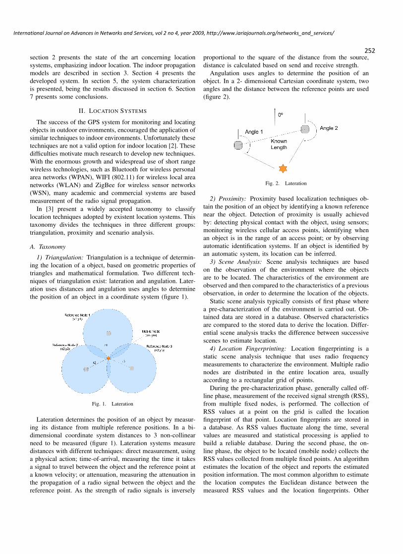
deterministic, such as nearest neighbor or neural networks andprobabilistic algorithms based on statistical learning theoryand Bayesian interference are also used.
III. INDOOR PROPAGATION MODELS
In radio frequency indoor location system, time and angleof arrival methods are not used because signals are affectedby the multipath effect. Triangulation is implemented based onthe attenuation methods, using models to relate the receivedpower with distance.
Indoor electromagnetic waves propagation, especially insidea building, is characterised by reflections, diffractions anddispersion in the internal structures. The transmitted signalsarrive to the receiver through multiple paths, originating fluc-tuations in the received signal. This effect, called multipathpropagation, is affected by the type of materials used in theconstruction of the building and by the surrounding objects.Therefore, it is very difficult to predict the strength of thereceived signal.
There are models that take into accounty the constructiveand destructive nature of multipath to relate the received powerwith the distance between transmitter and receiver. RayleighFading Model [4] and Rician Distribution Model [5] are widelyused, but they present some drawbacks. The Rayleigh FadingModel describes the small-scale rapid amplitude fluctuationsin the absence of a strong received component. It assumes thatall signals reaching the receivers have equal strength, whichis not a realistic approach. A dominant line-of-sight (LoS)component is not accounted for by this distribution. The RicianDistribuition Model takes in account that a strong path existsin addition to the low level scattered path. This model is veryappealing, but it is very difficult to determine its parameters,as this requires to physically isolate the direct wave from thescattered components [2].
A. Wall Attenuation Factor Model (WAF)The WAF model [2] is quite attractive, given its ability to
describe the slow fading phenomenon and the attenuation inthe signal propagation introduced in indoor environments. Itderives from the floor attenuation model (FAF) [6], wherean attenuation factor is used to estimate the signal intensityin different floors of a building. In the WAF model theattenuation factor permits to predict the behaviour of the signalpropagation, when walls are the main obstacle [2]. Equation1 indicates how the attenuation influences the received signalstrength.
P (d)[dBm] = P (d0)[dBm] − 10n log(
d
d0
)−{
nW ∗WAF , nW < CC ∗WAF ,nW ≥ C
(1)
In equation 1, n indicates the rate at which the attenuationof the signal increases with the propagation distance, P (d0) isthe received signal strength at a distance of reference d0 and d
is the distance between the transmitter and the receiver. In theattenuation factor, the C parameter accounts for the number ofwalls for which the attenuation factor (WAF) stops influencingthe signal; nW is the number of obstructions (walls) betweenthe transmitter and the receiver; and WAF is the value for theattenuation of each wall.
B. The Adjusted Motley-Keenan Model
The adjusted Motley-Keenan model [7] was developedbased on the Motley-Keenan model [8]. This last model,represented by equation 2, is similar to the WAF model, butdoes not limit the number of walls influencing the signlaattenuation. In equation 2, PLd is the the attenuation at 1meter of distance between transmitter and receiver, n theattenuation decay rate with distance, N the number of wallsbetween transmitter and receiver, and ki the number of type iwalls, having attenuation of Lwi.
PL(d)[dB] = PLd[dB] + 10n log(d) +N∑
i=1
kiLwi (2)
The adjusted Motley-Keenan model also considers the thick-ness of the walls. In equation 3, L0 is the attenuation ofa reference wall with thickness e0, and ei is the thicknessof a wall of type i placed between the transmitter and thereceiver. The adjusted term substitutes, i in equation 2, the
termN∑
i=1
kiLwi in order to account for the thickness of the
walls originating equation 4.
AdjustedTerm =N∑
i=1
kiL02log3
(eie0
)(3)
PL(d)[dB] = PLd[dB] +10n log(d)+N∑
i=1
kiL02log3
(eie0
)(4)
IV. DEVELOPED SYSTEM
The developed system creates a WSN with ZigBee technol-ogy to implement an indoor location system. This system wasdeveloped in order to have an automatic identification systemusing RFID. In the WSN one of the devices is mobile being thetarget of location. The other devices are placed in pre-definedpositions. The final objective is to place the mobile deviceon a person or object in order to determine his location andidentify him through WSN and RFID technology.
A. System Architecture
The ZigBee protocol emerges as a complement to the IEEE802.15.4 standard, guaranteeing reliability and safety as wellas a low energy consumption [14]. ZigBee using devicesshall have a maximum range of 150 meters, depending thisvalue of the environment and energy consumption of the usingapplication.
253
International Journal on Advances in Networks and Services, vol 2 no 4, year 2009, http://www.iariajournals.org/networks_and_services/

Fig. 3. Network Topology
The IEEE 802.15.4 standard defines three types of networktopologies: star topology, peer-to-peer topology and meshnetwork [14]. Figure 3 shows the three topologies.
The star topologies require at least one FFD (Full FunctionDevice) device functioning as network (WPAN - WirelessPersonal Area Network) coordinator. The communication isestablished between devices and the network coordinator.The WPAN coordinator is normally powered by the electricnetwork and the remaining devices (FFD or RFD (ReducedFunction Devices)) by batteries.
In peer-to-peer topologies there also exists a WPAN coordi-nator, being that in this topology all devices can communicatewith each other. The configuration can be found in controland industrial monitoring applications using WSNs. A meshnetwork is no more than a particular case of the peer-to-peertopology, where most of the devices are FFDs.
Given this, and because ZigBee distinguishes the conceptof physical devices (FFD, RFD) using the notion of logicaldevices, we propose a network that consists of a mobile devicethat acts as a ZigBee Coordinator and several fixed devicesacting as ZigBee End Devices. The ZigBee Coordinator isthe first type of logical device, assuming a role much similarto a coordinator in the IEEE 802.15.4 coordinator and isresponsible for: initiation, maintaining and manage a network.In the ZigBee hierarchy, next in line is the ZigBee End Devicethat is the final point in the network structure [15]. Theproposed network topology is very similar to the peer-to-peertopology in the IEEE 802.15.4, where the goal is to have allthe devices capable of communicate with each other.
We propose a system that is composed of a central serverthat executes the location algorithm as well as initiates thenetwork. The central server can be located in the mobiledevice, allowing the device to locate himself, or any otherlocation in the network being that because we are using ZigBeetechnology all the devices can communicate with each other.
B. Propagation Model
We use a propagation model based on the WAF propagationmodel [2], making the WAF parameter equal to zero (equation5). The walls are not always an obstacle between the mobileand the fixed devices. Therefore, we adopt equation 5 insteadof equation 1, but with different n and P (d0) than those usedin equation 1.
Figure 1 presents an example where obstructions can existin a certain direction but not in other directions, in the
circumference. Therefore, only at the distances and in thedirections where there is a presence of a wall the WAF factoris accounted for. Through this method it’s possible to obtaina wide range of different WAF values for the same distances.
During the first phase, where RSS values are collected todetermine n and P (d0) in equation 3, the RSS values thatare affected by the presence of a wall are identified (throughvisual inspection of the location environment).
To those RSS values the value of the WAF factor (previouslydetermined for respective distances and directions) will besubtracted in order to minimize the influence of the wallson the characterization of the RF signal in the locationenvironment. This way the WAF factor is taken into accountand it is reflected on the determined n and P (d0) parameters,instead of being a constant (equation 1) used at determineddistances in all directions [17].
P (d)[dBm] = P (d0)[dBm] − 10n log(
d
d0
)(5)
Fig. 4. Line of Sight
C. Location Algorithm
The goal for this location algorithm is to allow the locationof the mobile device within certain areas of the indoor envi-ronment. The proposed algorithm is not intended for a preciselocation of the mobile device but to distinguish where in acertain division of a room the device is located.
Knowing that, the developed location algorithm is dividedin two steps. Firstly, a propagation model is used to calculatethe distances between the fixed devices and the mobile device,based on the received signal strength indicator (RSSI). Thisphase involves the definition of the propagation models param-eters. These parameters are defined based on a previous char-acterization of the of RF signals in the location environmentin terms, by collecting the RSS values. This characterization ismuch like the off-line phase used in scenario analysis methods[3]. Next, knowing the distances between the fixed and mobiledevices and using a triangulation algorithm (see section D), itis possible to determine the location of the mobile device.
D. Triangulation Algorithm
To use the system, it is necessary to define the coordinatesystem and the position of the fixed nodes (base stations).We adopt a 2D system, assuming that all nodes are at thesame height. Knowing the positions of at least three fixed
254
International Journal on Advances in Networks and Services, vol 2 no 4, year 2009, http://www.iariajournals.org/networks_and_services/
devices and their distances to the mobile device it is possibleto calculate the coordinates (x,y) where the mobile device islocated.
In order to estimate the three fixed devices that are closer tothe mobile device, the centroid of a polygonal area as well asRSSI are used. The vertices of the polygon are fixed deviceswhich received a beacon message from the mobile device. Apreference index (FDI - Fixed Device Index) is then createdso that "best" fixed devices that received the beacon messagescan be chosen [16]. The FDI of FDi (Fixed Device) is definedby the following equation:
FDIi = (1− α)(
1−(
distcidistmax
))+ α
RSSIRi
RSSImax(6)
where distic are the Euclidian distances between the centroidof a polygon and FDi and α is a small number (0 ≤ α ≤ 1).The values for distmax and RSSImax are defined as:
distmax = max∀i{distci} (7)
and
RSSImax = max∀i{RSSIRi} (8)
where FDi is an FD which received a beacon message fromthe mobile device. Given FDIs, the triangulation algorithmselects the three FDs with the highest FDI values for triangu-lation.
We implemented the Dynamic Triangular Algorithm (DTN)[10]. It is well suited for small environments it is allowcomplexity algorithm a requires a reduced processing time.
The DTN algorithm needs at least three sensor nodes toestimate the location of mobile device. The method discardsthe worst RSSI values measured by the devices and uses thebest three to estimate location. It chooses the fixed devicewhich receives the greatest RSSI value and assumes thatthe mobile devices location is in the mapping circle of thatfixed device. The mapping circle is the estimation distance d1between the mobile device and the closest fixed device. TheDTN finds the angle θ on the mapping circle by using a costfunction to pick one that best matches the observed distance.The DTN has the following steps:
1) Generation of the mapping circle: It finds the possiblelocations of the mobile device (x1+d1cosθ, y1+ d1sinθ) on themapping circle by using the possible distances d2θ and d3θbetween mobile user and the fixed nodes.
2) The distance of the mobile device estimation: Finds theerror between estimation distances (d2 and d3) and possibledistances (d2θ and d3θ).
3) The coordinates of the mobile device approximation:Determines the cost functions at each angle θ and the θincreases 1 degree each time. The DTN then searches theminimum cost function, and the θ of the minimum costfunction is the estimation angle on the mapping circle. Theangle θ on the mapping circle is the estimation location of themobile device. Figure 5 describes the procedure of the DTNlocation algorithm.
Fig. 5. Dynamic Triangular Algorithm Procedure
E. Prototype Implementation
The final system will include fixed nodes and mobile nodes.Fixed devices will be placed in pre-defined positions. Theywill be implemented as embedded systems. Mobile nodes canbe implemented has embedded systems or objects and personsequipped with ZigBee tags. Mobile devices are the target forlocation and identification. Nodes will have a unique EPC(Electronic Product Code) identification number [9].
Five ZigBee nodes compose the developed prototype withfour fixed nodes and one mobile node. For prototyping pur-poses, we used a notebook connected to a ZigBee interfacethrough a RS-232 interface.
Fixed nodes and the ZigBee interface of the mobile nodeare PCB boards supporting commercially available ZigBee
255
International Journal on Advances in Networks and Services, vol 2 no 4, year 2009, http://www.iariajournals.org/networks_and_services/
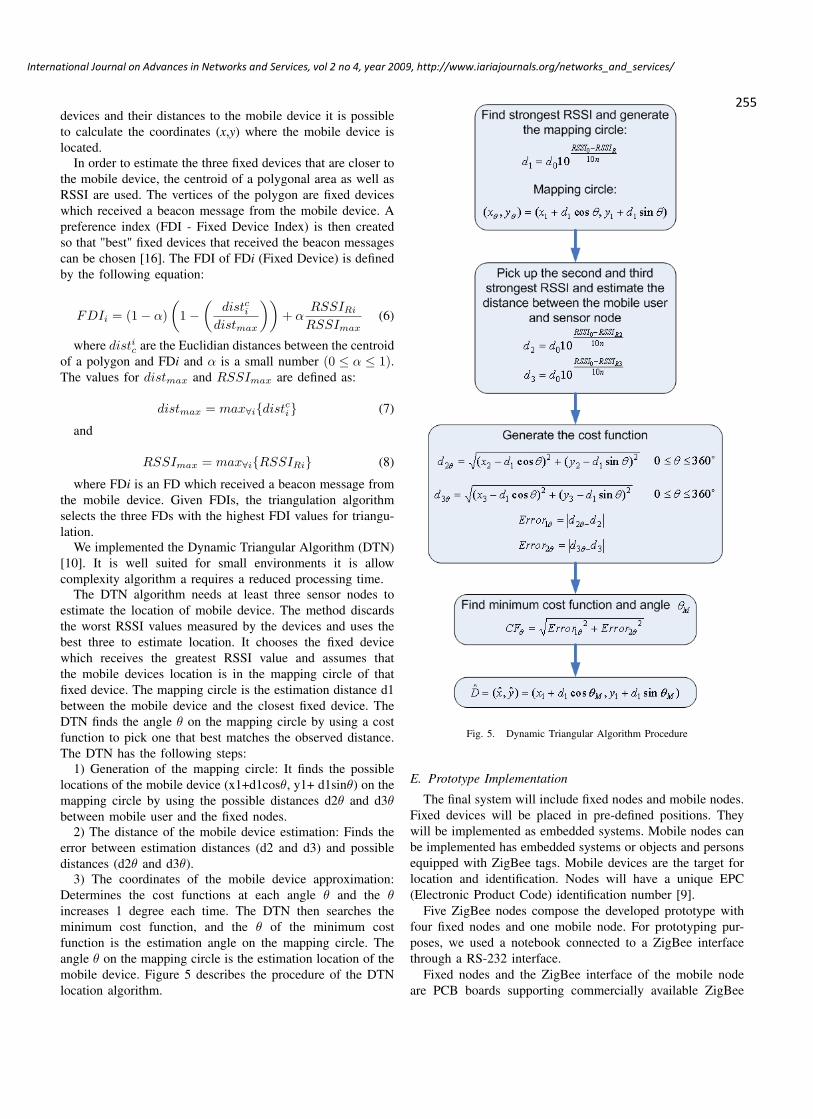
Fig. 6. Dynamic Triangular Algorithm
devices. The developed PCB board also include batteries, aRS232 interface and a USB interface. Programming of ZigBeedevices and EPC code assignment is done through RS232.The USB port is used to power the mobile device through anotebook. Fixed nodes are RFD (Reduced Function Device)programmed as ZigBee End Devices. They work indepen-dently and are powered by batteries. The mobile device is aFFD (Full Function Device), being programmed as a ZigBeeCoordinator. When starting, the mobile device transmits asignal in order to allow the fixed nodes, to detect it. Themobile device is responsible to transmit the received radiosignal strength indicator (RSSI) to the software applicationthat executes the location algorithm in order to determine themobile location.
The software application also initialises the wireless net-work, establishing the communication between ZigBee de-vices. Due to hardware limitations we connected the mobiledevice directly to a notebook, powering the device throughthe USB port and using the RS-232 port to communicate. Afuture and more advanced system would be controlled by aserver that would execute all the tasks, being the notebook nolonger needed.
V. SYSTEM CHARACTERIZATION
The prototype was installed and tested in a residentialenvironment. The location area is shown on Figures 7 and8. Table I shows the coordinates for each fixed device. EB1is located at the origin of the referential.
Fixed Devices Coordinates (x,y) in metersDevice 1 (0;0)Device 2 (4,8;5,8)Device 3 (0;5)Device 4 (3,7;0)
TABLE IFIXED DEVICES COORDINATES
As can be seen on Figure 7, we decided to use a smallarea. This approach minimizes the location error. In fact, theindoor range of ZigBee devices is limited and when distancesincrease location errors also increase. Although, it is possible
Fig. 7. Location Environment
Fig. 8. Set of small location environments
to locate objects in a much larger area, using several smallareas, as presented on Figure 8. Using similar small areaswith small obstruction also makes easier to characterize theenvironment. However, the number of fixed devices need tobe increased. (The number of devices shown in Figure 8 onlyhas the purpose of illustrating the general idea behind the useof small areas!)
In order to evaluate the capabilities and reliability of the lo-cation system we analyse the prototype in different situations:without the WAF factor, introducing the WAF factor and andusing an average value for the WAF factor.
The characterization of RF signals is essential to the locationsystem, only doing this it is possible to predict the signalbehaviour during propagation and determine the propagationmodel parameters (n and P (d0)). This characterization ismade through the collection of RSS values in a previous
256
International Journal on Advances in Networks and Services, vol 2 no 4, year 2009, http://www.iariajournals.org/networks_and_services/
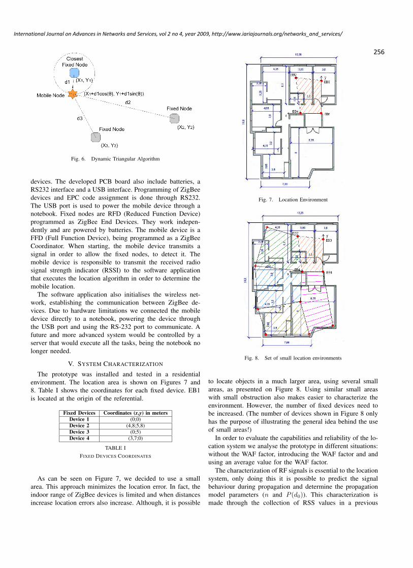
location stage (off-line).To determine the propagation model parameters, we fol-
lowed the scenario analysis described in [11]. Measuring thestrength of the received signal (RSS) at the fixed devices,transmitted by the mobile device, we repeated this processmoving the mobile device across the location area. RSS valueswere obtained in three fixed devices and, for each one, inthree different directions (as presented on Figure 9). The useof three devices instead of all four is enough to determine thepropagation model parameters.
Propagation model parameters were calculated for eachdevice individually and for all devices together. Therefore,there is a specific equation for each device and an equationthat can be used for all devices.
Fig. 9. Direction of collected RSS values
A. Parameter of attenuation WAFIn order to calculate the WAF value, RSS values were
measured, for the same distance, with and without a wall be-tween the fixed and mobile nodes. The WAF is the differencebetween the two RSS values. Table II presents WAF values ,for each device and all devices together, obtained for differentdistances.
Distance (meters) Device 1 Device 2 Device 32,5 - 4,25 dB -3 4,42 dB 11,5 dB 13,67 dB
3,5 17,42 dB - 6,5 dB4 - 18,08 dB 8,83 dB
TABLE IIWAF PARAMETERS
Table III shows the average value of WAF for each fixeddevice and for the set of values of all devices together.
B. Characterization of RF signals without WAFRSS values were collected in each fixed node and in all three
different directions. This RSS values permitted, by logarithmic
Fixed Devices Average WAFDevice 1 10,92 dBDevice 2 11,28 dBDevice 3 9,67 dB
All Devices 10,58 dB
TABLE IIIAVERAGE WAF PARAMETERS
regression, to calculate the attenuation ratio and the receivedsignal strength at the distance of 1 meter. Figure 10 illustratesthe use of logarithm regression and table IV presents the valuesobtained for the fixed devices.
Fig. 10. Collected values for device 3
Without WAF Attenuation Factor (n) RSS at 1m (P (d0))Device 1 2,382 -45,50 dBmDevice 2 3,637 -40,32 dBmDevice 3 2,806 -48,08 dBm
All Devices 3,027 -44,50 dBm
TABLE IVCALCULATED PARAMETERS WITHOUT WAF
With the calculated values in the tested situation it waspossible to plot the characteristic of the RF signal in terms ofthe distance using the theoretical model (propagation model)and compare it with the experimental collected RSS values.The following graphics (Figures 11 and 12) compare thetheoretical model with the average of the collected RSS valuesat different distances.
Fig. 11. Average Collected Values VS. Theoretical Model
C. Characterization of RF signals with WAFThis characterization is very similar to the first one and
uses the same collected RSS values, but with the difference
257
International Journal on Advances in Networks and Services, vol 2 no 4, year 2009, http://www.iariajournals.org/networks_and_services/
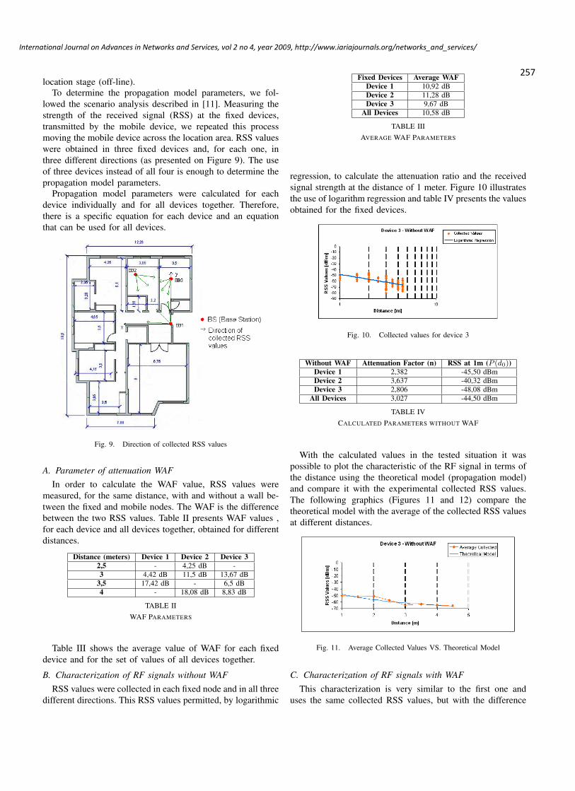
Fig. 12. Average Collected Values VS. Theoretical Model
that WAF values are now taken into account (Table I). TableV shows the calculated values of the propagation modelparameters through logarithmic regression and Figures 13 and14 show the graphics that compare the theoretical model withthe average of the collected RSS values at different distances.
With WAF Attenuation Factor (n) RSS at 1m (P (d0))Device 1 2,012 -45,77 dBmDevice 2 2,803 -41,12 dBmDevice 3 2,391 -48,07 dBm
All Devices 2,255 -45,21 dBm
TABLE VCALCULATED PARAMETERS WITH WAF
Fig. 13. Average Collected Values VS. Theoretical Model
Fig. 14. Average Collected Values VS. Theoretical Model
D. Characterization of RF signals with average WAF factor
This characterization is very similar to the first two and usesthe same collected RSS values, but with the difference thatthe average WAF values are now taken into account (Table
II) . The results were not very different then those fo thecharacterization of RF signals with WAF factor.
VI. RESULTS
After the characterizations the location algorithm was tested.In order to do that the mobile device was placed on twodifferent and random positions. The algorithm was testedwithout the introduction of WAF, with WAF and with theaverage value of WAF. The tests were also made for eachfixed device separately and for the set of values of all devicestogether, in this case all fixed devices were characterised bythe same propagation model equation. The tests revealed errorsfrom 2,5 to 0,25 meters when using the developed propagationmodel Tables VI and VII).
Point A Wout/ W/ All Wout/ All W/(1,8;4) m WAF WAF WAF WAF
Mob. Node (3,14;7,25) (2,29;6,52) (6,54;6,50) (3;-3,63)Coord.Coord. (1,34;3,25) (0,50;2,52) (4,74;2,50) (1,20;-0,37)ErrorDist. 3,51 2,57 5,36 1,26
Error
TABLE VILOCATION RESULTS FOR POINT A
Point B Wout/ W/ Avg. All Wout/ All W/(0,7;4) m WAF WAF WAF Avg. WAF
Mob. Node (0,54;5,65) (0,27;4,25) (0,72;5,86) (0,83;4,23)Coord.Coord. (-0,16;1,65) (-0,43;0,25) (0,02;1,86) (0,13;0,22)ErrorDist. 1,66 0,50 1,86 0,26
Error
TABLE VIILOCATION RESULTS FOR POINT B
Analysing Figures 11, 13 and 16 we can observe that,for certain locations, the introduction of the WAF parameterincreased the error. However, in general, the theoretical model(equation 5) is a good approximation of the collected RSSvalues. The graphics relative to the deviations of the collectedRSS values and theoretical model (Figures 16 and 18) confirmthe previous statement. A decrease in RSS values (whichtranslates into a decrease in error), can be observed on Figure15 when WAF parameter is introduced. This decreased is alsonoticed when using the average WAF parameter.
Its also verified in the standard deviation of the collectedvalues that at the same distance the fact that the RSS values arenot always the same, influences the parameters of the modelintroducing an additional error. Its also verified that when theset of values of all devices together is used to calculate themodel parameters it does not produce very different results ofthose presented when each fixed device has his own equation.
In general comparing the developed system with othersystems, that mainly use location fingerprint techniques, it is
258
International Journal on Advances in Networks and Services, vol 2 no 4, year 2009, http://www.iariajournals.org/networks_and_services/
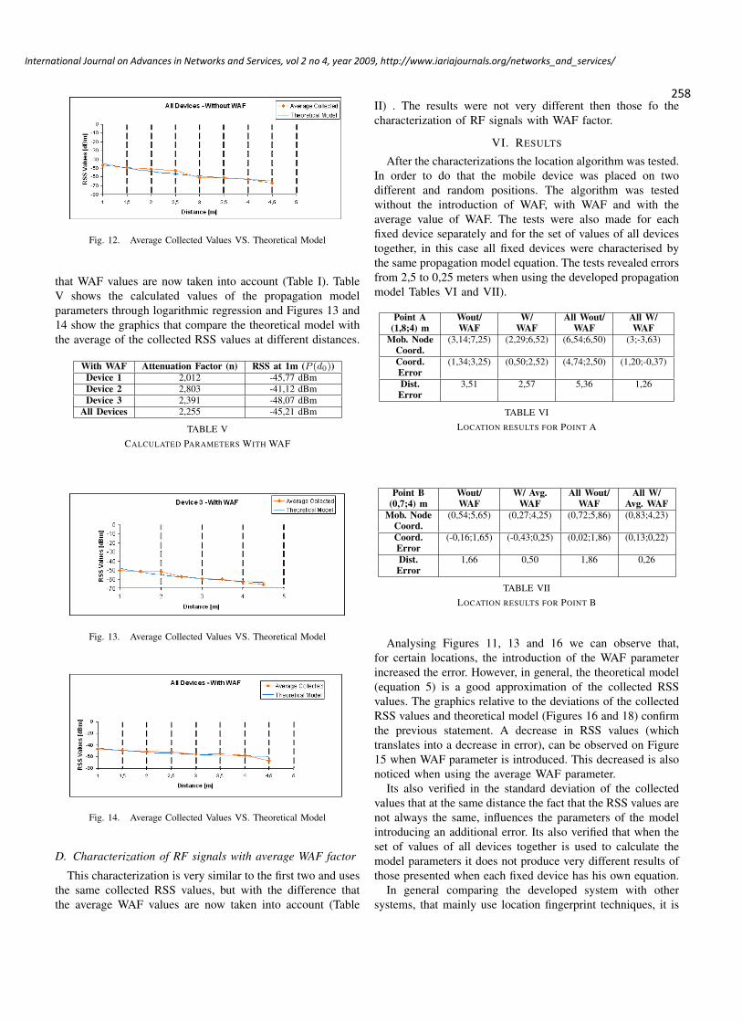
possible to assume that the developed system produces resultssimilar to other systems. Table VIII shows the typical errorof other location systems. Although the location environmentin which the systems were tested was larger than the oneused in this paper, the fact that location fingerprint techniquesusually produce more accurate results reinforces the goodresults achieved by the developed location system.
Location Systems Algorithm Type ErrorRADAR[2] Nearest Neighbour 2.13 metersYoussef[12] Bayesian 2.13 metersXIANG[13] Bayesian, RSS distribution model 1.83 meters
TABLE VIIICOMPARISON WITH LOCATION SYSTEMS
Fig. 15. Standard Deviation of the collected RSS values for device 3
Fig. 16. Deviation between the collected RSS values and theoretical modelfor device 3
Fig. 17. Standard Deviation of the collected RSS values for all devices
VII. CONCLUSION
This paper describes a location system for persons andobjects in an indoor environment, using ZigBee technology.
Fig. 18. Deviation between the collected RSS values and theoretical modelfor all devices
ZigBee nodes can function as RFID tags, having each one aunique EPC identification number. Sensors can be associatedwith the Zigbee wireless nodes to create applications for home,health and traffic control.
Location is determined, using a propagation model, basedon the WAF model, together with a triangulation algorithm.Tests demonstrate an increase in accuracy when the WAFparameter is used in the propagation model. Even the useof an average value for WAF or a set of values proved tobe effective. The same equation parameters can be used foreach fixed device, avoiding the need to collect RSS values foreach fixed device. This becomes very important when a newlocation system is to be installed in a new environment, wherethe building architecture is similar.
It is important to remark that signal characterization is cru-cial to ensure a good performance by the propagation model.The more values of RSS are collected the more accurate themodel becomes. On the other hand, it can be demonstrated thatwith a relative small number of collected values it is possibleto develop an effective flexible system, with errors from 2.5to 0.25 meters when using the developed propagation model.
Results also show that in the moment that the locationis initiated, it is important to collect several RSS values inorder to obtain an average RSS value in that time interval.The wide range of values that can be collected in the sameposition can vary enough to generate significant errors. Thisvariation is due to multipath that as the tendency to increasewith distance. The closer the devices are of each other the moreeasily can the propagation model be characterised. This factproves that the adopted concept of using a small set of locationenvironments that together make a bigger environment, is avalid option. This concept is especially interesting in a ZigBeeusing system, being that these networks can have thousandsof devices associated to them, reducing the distances betweenthe devices, all this at a low cost and low energy consumption.
A more advanced system would be able to track the mobiledevice instantaneously. The system could be controlled by acentral server that managed the ZigBee network and processedall the information needed to the location algorithm. In afuture system it would be possible to obtain not only aEPC identification number but a wide range of informationregarding the location environment.
259
International Journal on Advances in Networks and Services, vol 2 no 4, year 2009, http://www.iariajournals.org/networks_and_services/

REFERENCES
[1] "European Policy Outlook RFID", in Conf. RFID: Towards th Internet ofThings, Berlin, June 25-26, 2007.
[2] P.Bahl and V. N. Padmanabhan. "RADAR: An in-building RF-based userlocation and tracking system. in Proc. IEEE INFOCOM , 2000, pages775-784.
[3] J. Hightower and G. Borriello, "A Survey and Taxonomy of LocationSystems for Obiquitous Computing". Technical Report UW-CSE 01-08-03, University of Washington, Computer Science and Engineering, August24, 2001.
[4] H. Hashemi, The Indoor Radio Propagation Channel, Proceedings of theIEEE, Vol. 81, No. 7, pages 943-968 July 1993.
[5] S. 0. Rice, Mathematical analysis of Random Noise, Bell SystemsTechnical Journal, Vol. 23 (1944), Vol. 24 (1945).
[6] Seidel S. Y., Rappaport T. S.,914 MHz path loss prediction models forindoor wireless communications in multifloored buildings. IEEE Transac-tions on Antennas and Propagation, v. 40, no.2, pages 207-216, February1992.
[7] A. G. M. Lima and L. F. Menezes. Motley-Keenan Model Adjusted tothe Thickness of the wall, pages 180-182.
[8] Mikas F., Zvanovec S., Pechac P. Measurement and prediction of signalpropagation for WLAN systems. Czech Technical University in Prague,2002.
[9] "European Policy Outlook RFID", in Conf. RFID: Towards th Internet ofThings, Berlin, June 25-26, 2007.
[10] Ren C. Luo, Ogst Chen and Shi H. Pan. "Mobile User Localization inWireless Sensor Network Using Grey Prediction Method", Department ofElectrical Engineering, Nation Chung Cheng University, Taiwan, 2005.
[11] K. Kaemarungsi and P. Krishnamurthy, Modeling of Indoor Position-ing Systems Based on Location Fingerprinting. in Proc. IEEE INFO-COM,2004.
[12] M. A. Youssef, A. Agrawala, and A. U. Shankar, WLAN locationdetermination via clustering and probability distributions", in Proc. IEEEInternational Conference on Pervasive Computing and Communications(PerCom ’03), Dallas, Fort Worth, TX, Mar. 23-26, 2003, pp. 23-26.
[13] Z. Xiang, S. Song, J. Chen, H. Wang, J. Huang, and X. Gao, A wirelessLAN-based indoor positioning technology", IBM Journal of Research andDevelopment, vol. 48, no. 5/6, pp. 617-626, Sept./Nov. 2004.
[14] "Part 15.4: Wireless Medium Access Control (MAC) and Physical Layer(PHY) Specifications for Low-Rate Wireless Personal Area Networks(WPANs)", IEEE Standard for Information technology Telecommunica-tions and information exchange between systems, September 8, 2006.
[15] P. Kinney, "ZigBee Technology: Wireless Control that Simply Works",in Conf. Communications Design Conference, October 2, 2003.
[16] L. Yujin, P. Jaesung, "Practical Indoor Positioning System Using Re-ceived Signal Strength in IEEE 802.15.4 Networks", 2009.
[17] G. Gomes, H. Sarmento, "Indoor Location System using ZigBee Tech-nology", in Conf. SENSORCOMM 2009, June, 2009.
260
International Journal on Advances in Networks and Services, vol 2 no 4, year 2009, http://www.iariajournals.org/networks_and_services/
New Sensing Model for Wireless Sensor Networks
Peter Soreanu, Zeev (Vladimir) Volkovich
Software Engineering Department, ORT Braude College, Israel
[email protected], [email protected]
Abstract -The paper presents a new sensing model for
Wireless Sensor Networks. This model, named Circular Sector
Sensing Coverage, was first introduced by the authors at
SENSORCOMM 09 conference. It uses circular sectors with
variable central angles and radii. The purpose of the model is to
minimize the energy consumption of the sensing itself,
improving the energy balance of the sensor node (mote). This is
especially relevant when the sensing is done remotely, by
sending waves to detect intrusion or acquire data. Simulation of
this model shows energy savings versus previously published
schemes, suggesting the viability and the advantages of this new
sensing model. However, no analytical model was yet developed.
The present paper expands the scope of the previous one by
adding background information about known sensing models,
describing in greater details the algorithm used for simulation
and by presenting new and significant simulation results. The
obtained data confirms the advantages of this new sensing
model. The possible implementation of such a WSN may
significantly improve the energy-related performance of the
WSN, allowing the development of new applications and
improving the performance of existing ones.
Keywords: Wireless Sensor Network; sensing models;
sensing coverage; energy efficiency; circular sector
1. Introduction
The paper presents a new model of sensing coverage,
supposed to achieve a better efficiency of energy utilization
for remote sensing, by using an adaptable radii and angles
algorithm. Coverage areas of circular sector shapes,
adapted to the residual energy available, are used. The
model was first introduced by the authors in [1]. The
algorithm is intended to optimize the energy used for
sensing, in order to extend the life of the sensor network. It
does not assure a complete coverage of the area to be
sensed - an NP-hard problem. Although an analytical model
was not yet developed, the proposed model is interesting
and efficient, and is presented as such to the wireless sensor
networks community.
The Introduction section gives a succinct account of
WSN-related problems, with emphasize on energy-
efficiency related factors: placement and topology,
management, coverage, lifetime.
Research in WSN is advancing at a fast pace, as can be
seen in recent surveys of this topic - see [2][3].
Simultaneously, more and more actual deployments are
implemented. One of the main problems facing WSN
applications is the limited life span of the network. A
typical node (mote) is powered by a battery, which is
generally not field-replaceable. Also, energy harvesting
was developed only as a proof-of-concept, and is not yet a
viable option for real life implementations. A good survey
of energy-related problems may be found in [4].
A typical mote has three energy-hungry subsystems:
radio, processing and sensing unit. It is generally agreed
that most of the mote’s energy is required for
communication (Ɛc), followed by processing (Ɛp) and,
finally, sensing (Ɛs). The total lifetime of the WSN is a
function of their sum Ʃ, as shown in (1):
Ʃ = Ɛc + Ɛp + Ɛs (1)
The energy needed for communication Ɛc has the same
order of magnitude whilst the radio subsystem is
transmitting, receiving or in idle state. To reduce the
communication costs, two approaches were developed:
Duty-cycling, i.e., putting the radio in a sleep
mode and transmitting only when necessary. This
imposes the use of a sleep/wake-up algorithm to
coordinate their activities.
Data-driven approaches, which decrease the
amount of sensed data to be transmitted, by
optimizing the sampling time, and using data
fusion/aggregation/compression schemes.
The power consumption of the processing unit Ɛp is
generally three-four times of magnitude less than Ɛc .
Finally, research has shown that the energy consumption of
the sensing subsystem Ɛs may be significant, even greater
than the energy consumption of the radio or processing
subsystems [5]. The main factors are power hungry
transducers and A/D converters, long acquisition time and
the use of active sensors. The class of active sensors
contains sensors that use active transducers, as sonar, laser
or radar. They cover a dedicated sensing area, by sending
out a probing signal. It may acquire data such as remote
temperature, information about localization and tracking of
moving objects, or simple binary intrusion detection.
261
International Journal on Advances in Networks and Services, vol 2 no 4, year 2009, http://www.iariajournals.org/networks_and_services/

Sensing is strongly related not only to energy-efficiency,
but also to important problems such as area coverage and
connectivity. Both problems may be viewed as a measure
of quality of service in WSN. Maximizing coverage and
ensuring network connectivity is a difficult task and many
solutions were described [6][7]. The coverage of the sensed
field is conditioned by an optimum deployment of the
motes [8]. Various algorithms and approaches were
proposed [9-16]. The lifetime requirements of mote
deployment are related to their placement in the site to be
surveyed [17]. A comprehensive theoretical presentation of
the minimum-cost arrangement of the motes in order to
achieve the wanted coverage lifetime may be found in [18].
Analytical methods use Linear Programming, Voronoi–
diagram based heuristics or Delaunay triangulation in order
to achieve an energy-efficient coverage. While the coverage
problem is not solved for all cases and methods, good
results have been obtained for particular cases. One of the
best examples is described in [19] and [20].
The paper is organized as follows. In Section 2 we
present various models of sensing area coverage, with
emphasize on the disk model and his improvement, the
variable radii circular model. The new Circular Sector
Sensing Coverage (CSSC) model, which is a further
improvement, forms the object of Section 3. The simulation
environment for running the algorithm implementing this
model is described in Section 4. Section 5 discusses the
obtained results, while Section 6 proposes future research
paths and concludes the paper.
2. Sensing Area Coverage Models
From a functional point of view, there are two kinds of
sensing activities: local sensing and remote (or range)
sensing. The first one relates to local measurements, while
the late try to detect or measure a change of property of a
distant location or range. A typical local measurement may
be temperature, humidity, level of radioactivity, etc. in the
immediate proximity of the sensor. A typical remote
measurement may use ultrasound or a laser ray to detect an
intrusion or to track the velocity of a moving object.
Remote measurements make use of physical
characteristics of wave propagation. The time-of light
method uses pulses of energy transmitted toward the target,
and measures the time difference between the transmitted
and reflected signals. Another method use the relative
phase shift of these two signals. Lasers scanners may send
continuous frequency modulated signals, varying linearly
with time.
The results of the sensing may be deterministic or
probabilistic data. For local sensing, the probabilistic factor
is due to the precision range of the sensor. For remote
sensing, the probabilistic model takes into consideration the
inherent uncertainty of detections or measurements at
increasing distance.
2.1 Disk model of sensing This model defines the sensing area as a circle with
radius Rs for a sensor Si, constant for every i. This sensing
model is also known as the unit disk model [6][21].
It is generally accepted that the quality of sensing
decreases nonlinearly with the increase of the distance, like
in (2)
)2(),(
),(
PSdPSS
i
i
where S(Si, P) is the sensitivity of the sensor si at point
P, α and λ are parameters, and d(Si,P) is the distance
between the sensor and the point where the measurement is
done.
In the deterministic disk sensing model, sensing is done,
with a given accuracy, in and only in the area of a disk with
radius Rs, around sensor si. This is also called a binary
sensing model.
In the probabilistic model, the probability of detection
(or the accuracy of the measurement) varies as the distance
between the sensor si, and the point at coordinates (xi, yi),
P(xi, yi) increases. Figure 1 illustrates the different sensing
areas, while (3) defines the probability that a node will
detect a point P((xi, yi). The latest property is called the
probabilistic coverage of P(xi, yi), denoted )(, iyx sCii
.
Note that the quantity R is a measure of uncertainty in
detection , R < sR
)(, iyx SCii
Fig.1 Probabilistic disk sensing model
Generally, p is evaluated as aep , where
)(),( RRPSda si while ω and β are empirical
RRRif
RRRRRifp
RRRif
s
ss
s
0
)3(],[
1
262
International Journal on Advances in Networks and Services, vol 2 no 4, year 2009, http://www.iariajournals.org/networks_and_services/
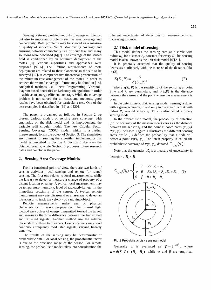
parameters that define the detection probability, when an
object is situated at a certain distance from the node.
Due to the fact that a point ),( ii yxP may lie in the
sensing area of more than one node, the total is defined as
in (4).
k
i
iyxyx SCCiiii
1
,, ))(1(1)( (4)
where χ is the set of nodes whose sensing ranges cover the
point },...,2,1,{),,( kisyxP iii .
This model reflects the sensing behaviour of devices like
ultrasound or infrared sensors.
2.2 Variable radii circular model While the disk model of sensing is simple and the
coverage may be relatively easily achieved by using an
equal-spaced grid deployment in an obstacle-less
environment, this model is not realistic and not energy-
efficient. It is not realistic because the variance in sensor
calibration and residual battery energy may substantially
vary from sensor to sensor during their lifetime. It is not
energy-efficient, because the overlapping of sensed areas
with more than the necessary sensing radius Rs causes a
waste of energy. Another argument is that a large sensing
radius will increase the consumption of energy, due to the
use of more sophisticated filtering and signal processing
methods. The later operation is required to improve the
signal-to-noise ratio, in order to achieve an energy-efficient
confidence level.
Various models of variable radii circular sensing models
were proposed, see [19][22]. They achieve an efficient
coverage of the sensed area, while using centralized or local
optimization algorithms. The basic idea is represented in
Figure 2. It can be seen that by using different radii (R1, R2,
R3), the sensed field can be better covered, with less
overlapping of sensed areas. Practical
implementations/simulations use discrete values for radii.
Fig. 2 Different sensing radii
It was shown [6] that this model, when compared to the
disk model, presents a more energy-efficient behavior,
especially in algorithms which try to solve the coverage
problem, i.e., the sensing through all the monitored area. It
allows for a more flexible and less redundant deployment
policy, while ensuring an optimal approach of solving
known coverage problems like
Minimal exposure path, which is a measure of
how well a sensed field is covered for detecting a
moving target.
Maximal breach path, defined as the highest
observability path in a sensing field
Maximal support path, which minimize the
distance from any point to the closest sensor.
2.3 Other sensing models In order to achieve even more energy-efficiency, and to
accommodate real-life scenarios, other sensing models
were proposed. A brief survey of the most significant ones
is given below.
The irregular sensing range model is based on extending
the variable radii circular model to a closed polygon. No
better energy efficiency is achieved, the sensing range
remaining the same. However, the analytical model
facilitates a better simulation of the WSN, efficiently
identifying fully covered sensors and discovering holes.
Centralized or distributed algorithms are used to analyze
the coverage problem [23].
Most of the WSN deployments are not truly two-
dimensional, but in the majority of cases the height is small
enough relatively to the length and width of the network.
When simulating the behavior of such a terrestrial network,
the third dimension (3D) of the motes may be safely
neglected. This is not the case with the underwater,
atmospheric or space deployment of WSN. The coverage
and connectivity aspects of 3D networks was also
researched, and the proposed solutions use generally
Voronoi tessellation to partition the space in hexagonal
prisms or rhombic dodecahedrons. [24]. These results have
energy-related practical consequences. Consider using
unmanned aircrafts for airspace surveillance, or underwater
unmanned autonomous vehicles for ocean surveillance.
Obviously, finding the optimal placement of vehicles,
minimizing their number while guaranteeing total coverage
of the space, makes a better use of the energy.
A possible approach to mitigate the coverage problem is
based on redeploying mobile redundant motes to uncovered
areas [25]. Nevertheless, obtaining location information in
a GPS-less wireless mobile sensor network demands a lot
of energy. This is due to heavy processing and extensive
message exchanges. A number of algorithms were devised
to alleviate these problems [26].
To be compared, each of the sensing models described
in Section 2 would ideally have a complete analytical
description. However, the majority of research papers
relates to specific aspects, like coverage, connectivity, most
exposed path, etc. The energy-effective aspect is generally
263
International Journal on Advances in Networks and Services, vol 2 no 4, year 2009, http://www.iariajournals.org/networks_and_services/
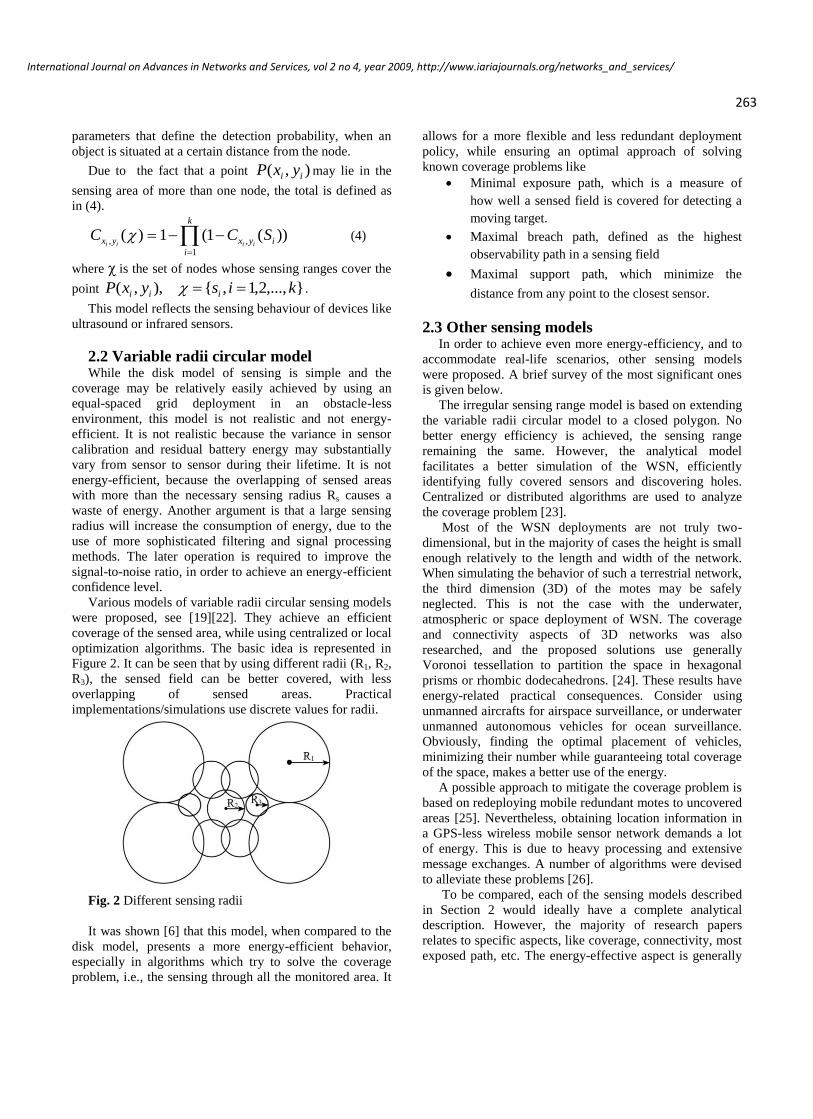
taken in consideration mostly by presenting results of
running simulations of these algorithms.
3. The Circular Sector Sensing Coverage
(CSSC) Model
Our work proposes a new sensing model - the Circular
Sector Sensing Coverage (CSSC) - based on circular
sectors with variable central angles and radii. The sensing
area is the portion of a circle enclosed by two radii and an
arc, whose values are set after analyzing the data received
from neighbor motes.
In Figure 3 an example of a possible partition of sensing
areas between three neighbor sensors (Sj, Sk, Sm) is given.
The sensed area between them is dynamically allocated as
follows:
Sensor Sj senses the area covered by the circular
sector SjAB, with radius R1 and circular angle θ1
(toward sensor Sk)
Sensor Sk senses the area covered by the circular
sector SkAB, with radius R2 and circular angle θ2
(toward the sensor Sj), and the area covered by the
circular sector SkCD, with radius R3 and circular
angle θ3 (toward sensor Sm )
Sensor Sm senses the area covered by the circular
sector SmCD, with radius R4 and circular angle θ4
(toward sensor Sk).
The same notation Si is used for the sensor itself and its
location. Observe the small overlapping areas between the
intersections of circular sectors.
Fig. 3 CSSC model schematics - an example
The CSSC model is based on exchange of residual
energy information between neighbor motes. The received
data is used to calculate the parameters of the circular
sectors covering the sensing areas. The goal is to maximize
the coverage, while optimizing the energy consumption.
Motes with more residual energy left in their battery may
increase the sensing area toward a neighbor with less
residual energy. The latest will correspondingly decrease
the sensing area in the direction of the neighbor that helps
him. The process is iterative, based on negotiations and
subject to convergence conditions. It is periodically
repeated during the lifetime of the WSN.
The following subsections describe the data exchanged
by motes, the implementation of the proposed CSSC
algorithm, and the visualization of the whole process.
3.1 Mote communication In order to establish the sensing areas of each mote,
they have to find their neighbors and send relevant
information. Finding neighbors is done by broadcasting
notification messages and assuming symmetric
communication. After that, they send localization data and
synchronization control commands. In the next stages,
actual energy-related and sensing area information is
exchanged. The relevant fields of such a packet contain
sender and receiver ID, sender location, operation code,
energy level and coverage percentages, maximum and
actual coverage distance, supplementary parameters.
The purpose of the communication is to:
receive enough data to calculate a variable called
StatParam, used in simulation - See (5).
notify neighbors about the current sensing area,
decided as a function of the value of StatParam
The variables are defined as follows:
StatParam is the relative residual energy of the
mote, function of the currently covered sensing
area.
EnergyLeft is the absolute value of the residual
battery energy.
CoverageConsum is the energy needed to sense
the covered circular sector area.
TimePeriod is the time interval between
StatParam evaluation
CrntCoverage is the area of the circular sensor
where this mote does the sensing
If this value is greater (by a predefined threshold) than
that of a neighbor node, the sensing area in his direction
will be increased.
3.2 Area coverage algorithm The algorithm used for the simulation of the CSSC
model is described, skipping only minor details. The
following steps are done for every mote:
Step 1
Broadcast and receive control messages from all
sensors. Based on localization information, build a list of
neighbors. A neighbor sensor is one which is situated closer
than twice the maximum sensing distance (radius). The
assumption is that the communication range is greater than
)5(
1
geCrntCoveraTimePeriod
nsumCoverageCo
EnergyLeftStatParam
264
International Journal on Advances in Networks and Services, vol 2 no 4, year 2009, http://www.iariajournals.org/networks_and_services/
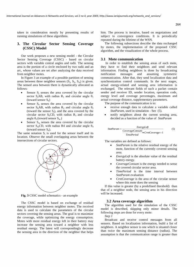
the sensing one, and location information is available and
part of the control message. Go to Step 2.
Step 2
Check the number of neighbors in the list. If no
neighbors are found, use the UnitDiskModel of sensing, i.e.,
circular sensing with maximum radius, and apply the
algorithm to the next mote. If only one neighbor is found,
go to Step 3. If more than 1 neighbors are detected, order
them according to their angular orientation: sort them
beginning with the least angle (from 0), clockwise. Go to
Step 3.
Step 3
For every neighbor, check if the maximum coverage
distance was received. If not, ignore the neighbor till
receiving this parameter. For all other neighbors, calculate
the radicals, i.e., the intersection lines of their maximal
radius sensing coverage circles. If radicals were found,
select and retain only the relevant ones (i.e., those that are
not hidden by other neighbors).
Fig. 4 Discarding radicals example
As can be seen in the example from Figure 4, the radical
KL of motes Sj and Sm is situated in the sensing area to be
covered by motes Sk and Sm. Consequently, radical KL will
be discarded, while radical MN will be retained for further
use. Go to Step 4.
Step 4
Calculate the StatParam values and compare them.
Decide for each neighbor if you can help to preserve its
energy reserve by increasing the covered sensing area in his
direction. Communicate the changed radical to the
neighbor. Do Step 3 for all neighbors and go to Step 5.
Figure 5 gives an example, showing how two equivalent
circular sector sensing areas ( SjPQ and SkPQ) may be
substituted by two asymmetric ones (SjRS and SkRS). This
allows mote Sk to consume less energy, at the expense of
mote Sj.
Step5
Eliminate overlapping of temporary calculated sensing
areas for pairs of motes, using the results of the sort done in
Step2. Do the sensing according to the newly defined
circular sectors.
Fig. 5 Moving the radical example Steps 1 to 5 are repeated periodically (in our simulation,
every 5 minutes) for all motes. In order to avoid
unnecessary changes, hysteresis was implemented when
evaluating the differences of the StatParam values.
3.3 Visualization of the process While running the algorithm described in the previous
subsection, "housekeeping" calculations are taking place,
to find and draw the current circular sectors. The results are
used mainly to dynamically draw the sensing areas of the
WSN on the screen. Furthermore, the obtained data is also
used in energy calculations and as help to check the
analytical model in work. These calculations doesn't affect
the concept of the CSSC model, being based on specific
geometric and programming implementations. The same
results may be obtained using different procedures. While
running interleaved with the computations needed to
implement the CSSC algorithm, these calculations are done
mostly during Step 4. Results from [27] were used for
clipping arcs.
After eliminating the unneeded radicals, belonging to
hidden neighbor motes (Step 3), a tentative temporary new
radical, defining the boundary of circular sectors for two
neighbor motes, is calculated (Step 4). A collection of
intersection segments is saved for each pair of neighbor
motes. The mote with the bigger sensing area will save
three segments, while the mote with a smaller sensing area
will save only one. Referring to Figure 5, mote Sj will save
segments PR, RS, and SQ - while mote Sk will save only
segment RS.
The next actions are needed to eliminate the ambiguity
of areas which may be covered by different pairs of
neighbor motes, i.e., they are overlapping. This is done by
comparing the relative positions of the saved intersection
lines, filtering them and even defining new ones.
Finally, the current circular sectors for the mote,
illustrating the received sensing areas, is decided. In the
example given in Figure 6, three circular sectors were
obtained, with the following parameters:
θ1=2π/3, 1
θ2= π/4, r2
θ3= π/4, r3, and r1> r2> r3
265
International Journal on Advances in Networks and Services, vol 2 no 4, year 2009, http://www.iariajournals.org/networks_and_services/
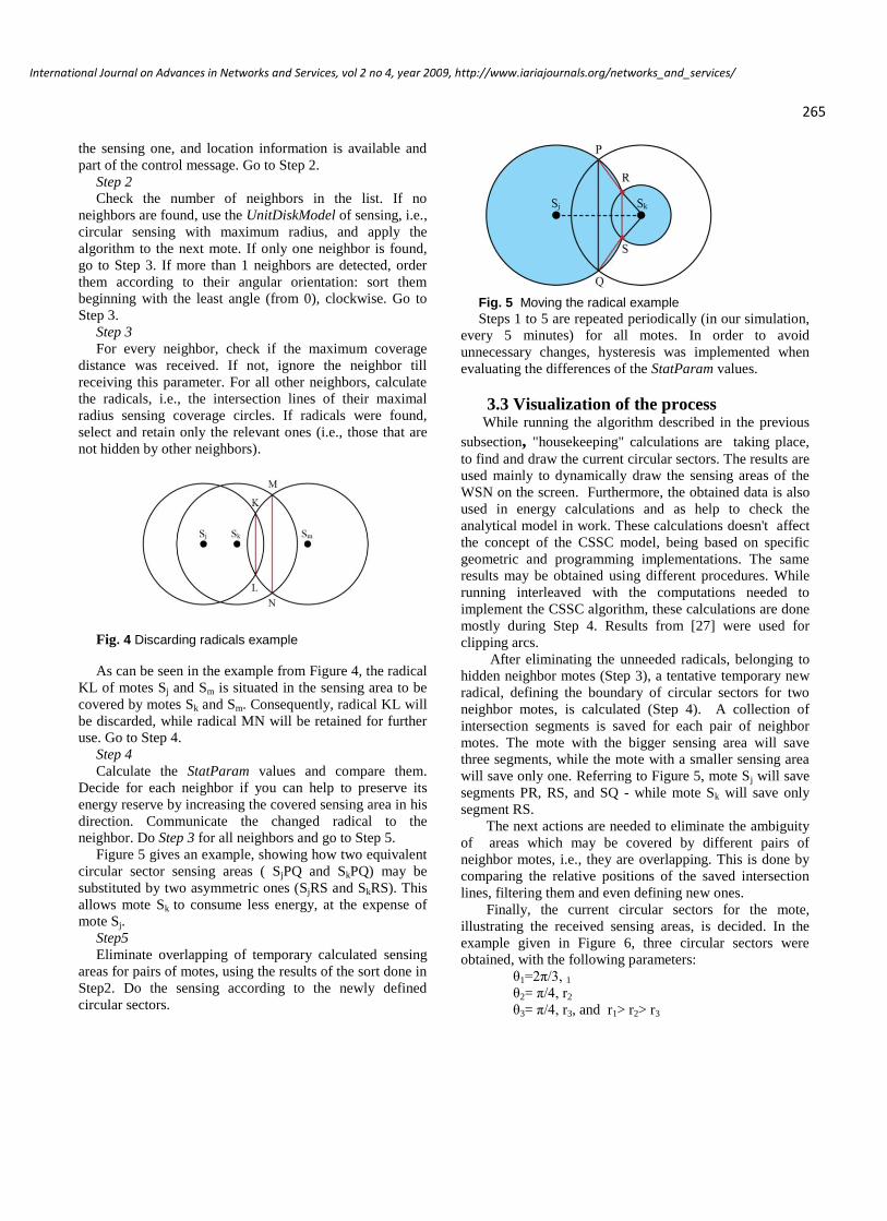
Fig. 6 Coverage example
It has to be noted that no complete coverage may be
guaranteed for a given deployment and residual energy of
motes. Conditions (6) and (7) hold for every mote:
∑ θi ≤ 2π (6)
where θi are the circular angles of the sensing circular
sectors of a mote.
ri + rj ≤ Ri + Rj (7)
where ri , rj are the current radii of neighbor motes Si and
Sj, while Ri , Rj are their maximum sensing radii.
The algorithm may be implemented centralized or as a
distributed process, at each mote. The energy of processing
overhead is obviously smaller than the energy used by
emitting light, electromagnetic or sound waves.
4. Simulation A dedicated simulation program was developed, based
on .NET and GDI+ environments. For the simulation data,
XML format was used. The simulator allows the
programming of the following WSN coverage sensing
models: disk unit (i.e., constant radius), circular (i.e.,
variable radii), and circular sector CSSC (i.e., variable radii
and angles). It has the usual features: mote deployment
methods, editing mote proprieties, save/import/export
scenarios, logs, result analysis, GUI and viewing area, etc.
The simulation may be checked in virtual real time, using
an adjustable virtual clock, which allows specifying a
desired running timeline.
The use of Opnet or ns-2 simulators was also
considered. However, when weighting their advantages
versus the flexibility of a purpose built dedicated simulator,
the last solution was preferred. The main reason was the
complexity of the CSSC model visualization.
Special care was given to chose the parameters of the
simulation. Data from similar simulations were evaluated.
The effects of routing protocols, which were not the object
of this research, were minimized (by using single hop
connections). A decision to not use, at this stage of the
research, heterogeneous motes, was also taken. The
planned testbed for WSN, to be built this year, also
influenced the choices. During the simulation process,
some of the settings and parameters were slightly changed,
mainly to achieve better visualization.
The main parameters and data for the simulated network
are given in Table 1.
Parameter Value
Maximum number of motes 100 to 200
Sensed area 60m x 60m
Network type Homogenous
Mote distribution Normal/manual
Initial capacity of the battery 1-4Ah
Drain current 40mA
Routing algorithm Single hop
Communication power/message - Tx 40mW
Communication power/message - Rx 5mW
Packet length (data and management) 1kB
Maximum sensing range 10m
Maximum sensing power (full circle,
maximum radius) 20mW
Central angle increments π/18
Radius increments 0.5m
Table1 Network and mote parameters
Typical timing parameters may be found in Table 2.
Parameter Value
Location transmission 10s after start
First data transmission 30s after start
Data transmission intervals 10s
Neighbor motes negotiations interval 5s Table 2 Timing parameters
266
International Journal on Advances in Networks and Services, vol 2 no 4, year 2009, http://www.iariajournals.org/networks_and_services/

The main metrics used are enumerated in Table 3.
Metric Defined as
Data reports
Quantity of data sent by
all motes
Redundant data
Measurement already sent
by neighbor motes
Application messages Number of data messages
Management messages
Number of management
messages
Number of motes
Current number of active
motes
Table 3 WSN simulator metrics
For the purpose of simulation, all messages were defined
as having the same number of bits.
The simulator may be relatively easy expanded to
process new sensing models, mote parameters, running
conditions, measurements, and visualizations. A typical
screenshot, representing a partial view of the WSN area
may be seen in Figure 7. It illustrates the initial phase of the
algorithm. The weight of the red rectangles is proportional
to the residual energy of the batteries.
The simulated scenario used a uniform random
distribution of motes, while the virtual simulated time was
1000 hours. Three algorithms were implemented: unit disk,
circular model, and circular sector (CSSC) model. A
variable number of sensors were deployed (between 100
and 200), and performance differences were observed and
will be discussed in the next section.
Fig. 7 Network View screen – partial initial field snapshot
5. Results Extensive running of the CSSC algorithm were
done. The results were compared to both the disk unit
and the circular model. The life span of sensors, in
various deployment situation and energy
reserve/consumption assumptions were calculated
during the simulations. The CSSC algorithm shows
performance improvements of the lifetime of
simulated WSNs.
Typical results are presented in Figure 8 and
Figure 9. Although different number of motes were
used in simulations, the graphs represent the
minimum and the maximum number of motes only.
Running of algorithms can be seen in two situations:
deployment of 100 motes (Fig. 8) and 200 motes
267
International Journal on Advances in Networks and Services, vol 2 no 4, year 2009, http://www.iariajournals.org/networks_and_services/
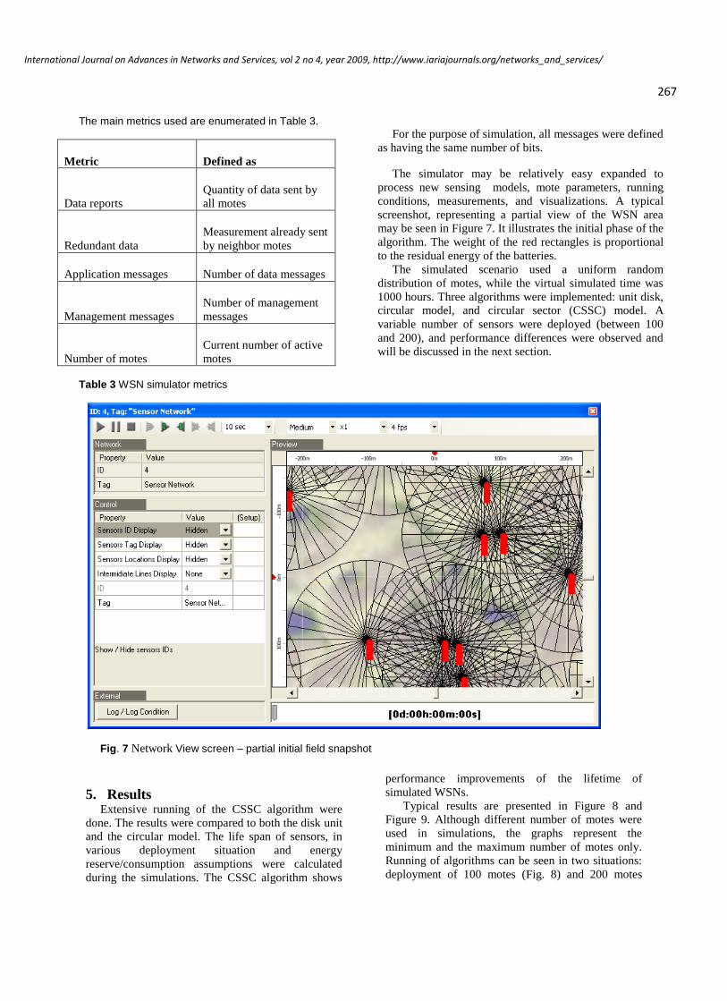
(Fig. 9) in the same field. Both graphs plot the
number of active motes, i.e., the motes with still
residual battery energy as function of running time.
As a consequence of the single-hop communication
model adopted, the communication range is supposed
to be always operational till the sink, and therefore
the possible loss of the transmission connectivity is
not an issue. It can be seen that the CSSC model is
consistently more energy-efficient.
Interpreting the chart from Figure 9, it can be seen
that after 1000 hours (simulated time), the WSN field
utilizing the CSSC model had about twice more
active nodes left, compared to the circular model.
The CSSC model demonstrated, under the same
conditions, a 50% increase in the number of active
nodes also vs. the circular sensing model.
An interesting performance difference emerged
from the simulations obtained by running 100 vs. 200
motes. The chart in Figure 9 shows shorter life-spans
of WSN with 200 motes, compared to WSN with
100motes. The advantage of CSSC model, while
observed, is less significant. A possible explanation
may be the differences in the energy dissipation
mechanisms required by the three sensing models.
The energy-efficiency of the disk unit sensing model
was not influenced by the number of motes, while the
circular model was slightly affected and the CSSC
model even more.
We have found a strong negative correlation
between the density of motes in the WSN field and
the energy-efficiency of the CSSC model. This model
is less energy efficient for densely populated WSN
fields. As can be seen in Fig. 10, a strong positive
correlation exists between the motes density and the
number of exchanged management messages. The
presence of more neighbors in the sensing range of a
mote implies an increased number of negotiations to
establish the mutual optimal sensing areas. While this
density decreases with time, it contributes to the
energy consumption balance of the WSN.
Fig. 8 Sensor field life – 100 motes
Fig. 9 Sensor field life – 200 motes
Fig. 10 Number of management messages (CSSC
sensing model)
When varying the data transmission intervals,
slightly modified simulation results were obtained.
As expected, the maximum rate of 5s produced the
greater energy consumption, while the minimum
simulated rate of 15s presented a much more energy-
efficient behavior. The results of these simulations
are plotted in Figures 11(a), 11(b), and 11(c). They
show the decrease of the number of remaining active
motes vs. simulated time, when varying the data
transmission intervals, for 100 motes initially in the
WSN field. It may be seen that the relative
performance of the three sensing models remains
invariant, and no significant advantage of CSSC may
be reported. At the beginning of the simulation, the
increased energy consumption has no influence on
motes depletion, due to the still enough existent
residual energy.
0
20
40
60
80
0.025 0.035 0.045 0.055 0.065M
ess
age
s/m
ote
/min
Motes density (motes /sqm)
0
50
100
150
0
200
400
600
800
1000
Nr.
of
mo
tes
Time (hours)
Disk
050
100150200250
0
200
400
600
800
1000
Nr.
of
mo
tes
Time (hours)
Disk
Circular
CSSC
268
International Journal on Advances in Networks and Services, vol 2 no 4, year 2009, http://www.iariajournals.org/networks_and_services/
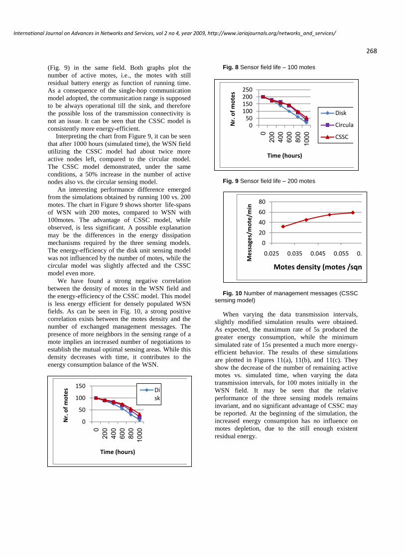
Fig. 11(a) Varying the data transmission intervals
(5s to 15s) – Disk model/100 motes
Fig. 11(b) Varying the data transmission intervals
(5s to 15s) – Circular model/100 motes
Fig. 11(c) Varying the data transmission intervals
(5s to 15s) –CSSC model/100 motes
During the simulation runs, we also changed the
rate of negotiation management messages between
neighbor motes. For the disk model, where no
management messages are used, obviously no
performance change occurred. For the circular
sensing model, the simulation showed a significant
performance worsening when increasing the rate of
these messages, as can be seen in Figure 12(a). The
increased number of management messages
exchanged between neighbor motes, in order to
negotiate a possible change of the sensing radii,
achieved an increased energy-consumption, resulting
in a bigger depletion rate. Simulation showed that the
expected improvement of the sensing energy needs
was not achieved.
When decreasing the sensed data transmission rate
beyond a certain value, a similar increase of the
energy consumption was observed. This result is the
consequence of using a not actualized and therefore
less efficient set of sensing radii. Establishing an
optimal rate is obviously needed. It have to be noted
that (because of the one-hop communication model
implemented) the simulation neglected data fusion
scenarios, in which case the negative influence of
increased data transmission rates may be alleviated.
A similar behavior was observed for the CSSC
model. From Figure 12(b) it can be seen that the
influence of varying the rate of the exchanged
messages is even greater than for the circular model.
The simulation used the same no. of bits for both
models. Therefore, this result may be attributed to the
following two factors:
Increased processing time, calculating not
only the radius, but also the value of the angle
and the position of the arc.
Less energy-efficient sensing optimization.
While the CSSC model is more energy-efficient than
the circular model, it is also more sensible to timing
considerations.
Fig. 12(a) Varying the neighbors’ negotiation
interval (2s to 12s) – Circular model/100 motes
0
20
40
60
80
100
120
0 2004006008001000
Nr.
of
mo
tes
Time (hours)
5s
0
20
40
60
80
100
120
0 2004006008001000
Nr.
of
mo
tes
Time (hours)
5s
0
50
100
150
0 500 1000
Nr.
of
mo
tes
Time (hours)
0
50
100
150
0 500 1000
Nr.
of
mo
tes
Time (hours)
269
International Journal on Advances in Networks and Services, vol 2 no 4, year 2009, http://www.iariajournals.org/networks_and_services/

Fig. 12(b) Varying the neighbors’ negotiation
interval (2s to 12s) - CSSC model/100 motes
From the results of these simulations, it can be
seen that the number of active motes remains
constantly greater when using CSSC, if the rate of
management messages is below a certain level. This
level has to be found empirically for every specific
WSN using this sensing model.
Comparing graphs for this worst-case scenario, as
represented in Figure 13, it can be seen that for
improperly chosen parameters, the energy-efficiency
of the CSSC model may be even lower than that of
the Circular model.
Fig. 13 Circular and CSSC sensing models –
worst case scenario
Even if sometimes, at the beginning of the WSN
activity, the use of CSSC model seems less energy-
efficient than the circular model, toward the end of
life-span of the networks it performs better.
Significant improvements vs. the circular sensing
model were obtained after 1000 simulated hours of
sensing/transmitting. The simulation was stopped at
this time interval, due to the fact that the remaining
number of motes was not enough to effectively cover
the sensed field. However, it has to be noted that the
simulator has no facilities to check the connectivity
of the covered areas. As such, although the lifetime
of the WSN was obviously increased, it was not
possible to accurately assess coverage data.
6. Conclusion and Future Work
A new model of sensing coverage for active
sensors, based on circular sector sensing coverage –
CSSC, was developed. The performance of this
model was checked vs. previously published
schemes, using a dedicated simulation program.. The
results of the simulations showed energy savings,
suggesting the viability and the advantages of this
new sensing model. After 1000 hours of simulated
sensing and data reporting, up to a 50% increase in
the number of active motes was observed. The best
performance, from an energy-efficiency point-of-
view, was obtained in a sparsely populated WSN
field, using a moderate rate of management
messages.
The possible implementation of such a WSN may
improve the energy-related performance of the WSN,
allowing the development of new applications and
improving the performance of existing ones. There
are a lot of such applications, civilian or military
alike, which implement some remote discovery,
localization or tracking activities.
We want to stress again, that no analytical model
exists yet for CSSC. However, it is a new sensing
model, which as observed during simulations, shows
energy-efficiency related performance improvements
vs. other known sensing models.
Suggested future possible research topics include:
Describing analytically the CSSC model.
Minimizing the required communication
overhead, to further increase the energy
savings.
Maximizing the coverage area, while using
minimal energy.
Studying the minimal exposure path, to check
its behavior vs. other sensing models.
Testing the connectivity of sensing areas, in a
multi-hop communication environment.
Researching the behavior of the model in a
mobile WSN environment
At this stage, our work concerning the circular
sector sensing coverage model CSSC concentrates
on:
Developing an accurate and complete
analytical model.
Defining the optimal rate of the management
messages.
0
50
100
150
0 500 1000
Nr.
of
mo
tes
Time (Hours)
0
50
100
150
0 500 1000
Nr.
of
mo
tes
Time (hours)
C…C…
270
International Journal on Advances in Networks and Services, vol 2 no 4, year 2009, http://www.iariajournals.org/networks_and_services/
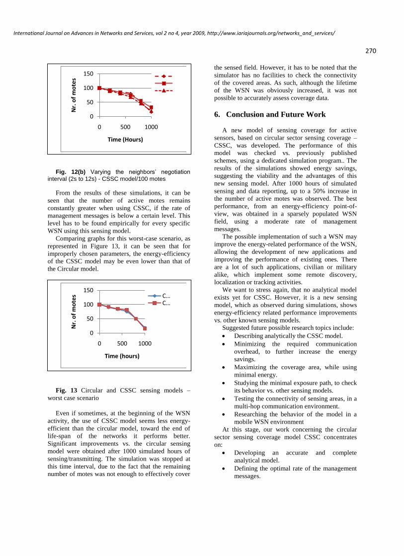
Adding new metrics and functions to the
simulator, for a more accurate modeling of
sensing models and a deeper understanding of
the behavior of the circular sector CSSC
model.
.
Acknowledgments
We would like to thank the students who
programmed the simulator and implemented the
CSSC model, especially Itzik Shoshan and Itay
Ronen.
References [1] P. Soreanu and Z. Volkovich, “Energy-efficient
circular sector sensing coverage model for wireless
sensor networks”, Proceedings of the 3rd International
Conference on Sensor Technologies and Applications,
June 2009, Athens, Greece pp.229-233,
doi:10.1109/SENSORCOMM.2009/45
[2] J. Yick, B. Mukherjee and D. Ghosal, "Wireless
sensor network survey", Computer Networks: The
International Journal of Computer and Telecom-
munications, Elsevier, vol.52(12), August 2008,
pp.2292-2330, doi:10.1016/j.comnet.2008.04.002
[3] V. Potdar, A. Sharif and E. Chang, “Wireless sensor
networks: a survey”, Proc. 2009 International Conf.
on Advanced Information Networking and Appl.
Workshops, May 29-29, Bredford, UK, pp. 636-641,
doi:10.1109/WAINA.2009.192
[4] G. Anastasi, M. Conti, M. Di Francesco and A.
Passarella," Energy conservation in wireless sensor
networks ", Ad Hoc Networks, Elsevier, vol. 7(3),May
2009, pp. 537-568, doi:10.1016/j.adhoc.2008.06.003
[5] C. Alippi, G. Anastasi, M. Di Francesco and M.
Roveri, “Energy Management in Wireless Sensor
Networks with Energy-Hungry Sensors”, IEEE
Instrumentation and Measurement Magazine”, IEEE
Press, vol.12, April 2009, pp. 16-23,
doi:10.1109/MIM.2009.4811133
[6] Ghosh and S. K. Das, "Coverage and connectivity
issues in wireless sensor networks ", Pervasive and
Mobile Computing, Elsevier, vol.4(3), June 2008, pp.
303-334, doi:10.1016/j.pmcj.2008.02.001
[7] D. Zorbas, D. Glynos, P. Kotzanikolaou and C.
Douligeris, "Solving coverage problems in wireless
sensor networks using cover sets", Ad Hoc Networks,
Elsevier, vol. 8(4), June 2010, pp.400-415, in press,
doi:10.1016/j,adhoc.2009.10.003
[8] M. Younis and K. Akkaya, "Strategies and techniques
for node placement in wireless sensor networks", Ad
Hoc Networks, Elsevier, vol.6(4), June 2008, pp. 621-
655, doi:10.1016/j.adhoc.2007.05.003
[9] C.-F. Huang, Y.-C. Tseng and H.-L. Wu, "Distributed
protocols for ensuring both coverage and connectivity
of a wireless sensor network", ACM Transactions on
Sensor Networks, vol. 3(1), March 2007, 24 pp ,
doi:10.1145/1210669.1210674
[10] C.-Y. Chang and H.-R. Chang, "Energy-aware node
placement, topology control and MAC scheduling for
wireless sensor networks", Computer Networks: The
Int'l Journal of Computer and Telecommunications,
Elsevier, vol.52(11), August 2008, pp. 2189-2204,
doi:10.1016/j.comnet.2008.02.028
[11] C.-F. Wang and J.-W. Ding, "The optimum sensor
redeployment scheme using the most frangible cluster
sets", Computer Communications, Butterworth-
Heinemann, vol. 31(14), September 2008, pp.3492-
3502, doi:10.1016/j.comcom.2008.06.004
[12] B.Wang, C,-F. Hock, B, Lim, "Layered diffusion-
based coverage control in wireless sensor networks",
Computer Networks: The International Journal of
Computer and Telecommunications Networking,
Elsevier,vol. 53(7), May 2009, pp. 114-1124,
doi:10.1016/j.comnet.2008.12.013
[13] C.-F. Huang and Y.-C. Tseng, “The coverage problem
in a wireless sensor network”, Mobile Networks and
Applications, Springer, vol. 10(4), August 2005, pp.
519-528, doi:10.1007/s11036-005-1564-y
[14] C.-H. Wu, K.-C. Lee and Y.-C. Chung, "A Delaunay
triangulation based method for wireless sensor net-
work deployment", Computer Communications,
Butterworth-Heinemann, vol. 30(14-15), Oct. 2007,
pp.2744-2752, doi:10.1016/j.comcom.2007.05.017
[15] Y.-R. Tsai, "Coverage-preserving routing protocols
for randomly distributed wireless sensor networks",
IEEE Transactions on Wireless Communications,
IEEE Press, vol. 6(4), April 2007, pp. 1240-1245,
doi:10.1109/TWC.2007.348320
[16] I. G. Siqueira, L. B. Ruiz, A. A. F. Loureiro and J. M.
Nogueira, "Coverage area management for wireless
sensor networks", International Journal of Network
Management, John Wiley & Sons, vol.17(1), January
2007, pp. 17-31, doi:10.1002/nem.604
[17] J. Wang and N. Zhong, "Minimum-cost sensor
arrangement for achieving wanted coverage lifetime",
International Journal of Sensor Networks,
Inderscience Publishers, Geneva, vol. 3(3), May
2008, pp. 165-174, doi:10.1504/IJSNET.2008.018481
[18] T. H. Lai and S. Kumar, "Foundations of coverage in
wireless sensor networks", Ohio State University Pub.,
2006, ISBN:978-0-542-78170-4
[19] J. Wang and S. Medidi, "Energy efficient coverage
with variable sensing radii in wireless sensor
networks", Proc. of the Third IEEE International
Conference on Wireless and Mobile Computing,
Networking and Communications (WiMob 07),
Oct.2007, White Plains, NY, IEEE Computer Society,
vol2, pp. 61-68, doi:10.1109/WIMOB.2007.30
[20] C.T. Vu and Y. Li, "Delaunay-triangulation based
complete coverage in wireless sensor networks", Proc.
of the 2009 IEEE International Conference on
Pervasive Computing and Communications (PerCom
2009),March 2009, IEEE Computer Society, pp.1-5,
doi:101109/PERCOM.2009.4912842
[21] S.-C. Lee, S.-B. Shin, H.-S. Hwang and C.-S. Kim, “A
Study on the Circular Sensing Model with a Low
271
International Journal on Advances in Networks and Services, vol 2 no 4, year 2009, http://www.iariajournals.org/networks_and_services/

Power Profile in Wireless Sensor Networks”, Proc. of
5th ACIS International Conference on Software
Engineering Research, management & Applications
(SERA 2007), 20-22 Aug. 2007, Busan, S. Korea, pp.
616-622, doi:10.1109/SERA.2007.32
[22] M. Cardei, J. Wu and M. Lu, "Improving network
lifetime using sensors with adjustable sensing ranges",
International Journal of Sensor Networks,
Inderscience Publishers, Geneva, vol. 3(1/2), January
2006, pp. 41-49, doi:10.1504/IJSNET.2006.010833
[23] A. Boukerche and X. Fei, "A coverage-preserving
scheme for wireless sensor network with irregular
sensing range", Ad Hoc Networks, Elsevier, vol.5(8),
pp. 1303-1316, doi:10.1016/adhoc.2007.02.020
[24] S.M.N. Alam and Z.J. Haas, “Coverage and
connectivity in three-dimensional underwater sensor
networks”, Wireless Communications & Mobile
Computing, John Wiley & Sons, vol8(8), Oct.2008,
pp. 995-1009, doi:10.1002/wcm.v8:8
[25] Y.-C. Wang and Y.C. Tseng, "Distributed deployment
schemes for mobile wireless sensor networks to ensure
multilevel coverage", IEEE Transactions on Parallel
and Distributed Systems, vol. 19(9), pp.1280-1294,
doi:10.1109/TPDS.2007.70808
[26] W.Y. Chang, C.-H. Wang, L. C. Hsu, K. J. Cheng.,
“Coverage algorithms in GPS-less wireless mobile
sensor networks”, Proc. Intl. Conference on Mobile
Technology, Applications, and Systems (Mobility ’08),
September 10-12, Yilan, Taiwan, ACM Publisher,
doi:10.1145/1506270.1506368
[27] C. J. Van Wyk, “Clipping to the Boundary of a
Circular-Arc Polygon”, Computer Vision, Graphics,
and Image Processing, vol. 25(3), March 1984, pp.
383-392
272
International Journal on Advances in Networks and Services, vol 2 no 4, year 2009, http://www.iariajournals.org/networks_and_services/
FastM: Design and Evaluation of a Fast Mobility Mechanism for Wireless MeshNetworks
Luís Couto, João Paulo Barraca, Susana Sargento, Rui L. AguiarUniversidade de Aveiro, Instituto de Telecomunicações, Aveiro, Portugal
{lcouto, jpbarraca} @av.it.pt, {susana, ruilaa} @ua.pt
AbstractAlthough there is a large volume of work in the literaturein terms of mobility approaches for Wireless MeshNetworks, usually these approaches introduce highlatency in the handover process and do not support real-time services and applications. Moreover, mobility is de-coupled from routing, which leads to inefficiency to bothmobility and routing approaches with respect to mobility.In this paper we present a new extension to proactiverouting protocols using a fast mobility extension, FastM,with the purpose of increasing handover performance inWireless Mesh Networks. With this new extension, a newconcept is created to integrate information betweenneighbor wireless mesh routers, managing locations ofclients associated to wireless mesh routers in a certainneighborhood, and avoiding packet loss during handover.The proposed mobility approach is able to optimize thehandover process without imposing any modifications tothe current IEE 802.11 MAC protocol and use unmodifiedclients. Results show the improved efficiency of theproposed scheme: metrics such as disconnection time,throughput, packet loss and control overhead are largelyimproved when compared to previous approaches.Moreover, these conclusions apply to mobility scenarios,although mobility decreases the performance of thehandover approach, as expected.
Keywords: Fast Mobility, mesh networks, MeshDV,neighboring tables, handover signaling.
1. Introduction
Wireless Mesh Networks (WMNs) are dynamically self-organized and self-configured networks, where terminalsare connected through routers in a mesh topology. WMNsincrease the capabilities of ad-hoc networks, such asrobustness, power management, reliable service coverageand optimized node mobility (Figure 1). Coverageincreases automatically, allowing a continuous addition ofterminals and a self-adapting topology. In the meshinfrastructure there are two types of devices: the WirelessMesh Routers (WMRs) and the Wireless Mesh Terminals(WMTs). WMRs are devices able to provide multi-hoptransport mechanisms enabling communication between
the terminals in the same or in different WMNs. Aterminal can be any type of device with a wirelessinterface (typically 802.11a/b/g), whether mobile orstationary. In the particular case of the WIP project [2],where this work was performed, terminals will mostly becomprised of laptops, desktop computers or PDAs, allsupporting 802.11a/b/g.
In WMNs, terminal mobility occurs whenever a clientassociated to an access point (or WMR directly) wants tochange its point of attachment. To maintaincommunication with other terminals, it needs to constantlyinform active correspondent nodes about its currentlocation. Any mobility solution designed to thesenetworks must be able to quickly update terminalslocation information with low overhead yet effectively,creating a reliable, non-interrupted communicationbetween nodes. Cellular technologies, such as the onesused in current GSM and UMTS networks, are able tosupport seamless connectivity between neighbor points ofattachment. WMNs, typically using 802.11, are unable tomeet the requirements for voice continuity without furthersolutions.
In this paper, which is an extended version of the workpresented in [1], we propose a new mobility mechanismfor WMNs denoted as FastM, Fast Mobility supportextension for WMNs, an evolution of MeshDV [3] andEnhanced Mobility Management (EMM) [4], inheritingthe basic functional aspects, but using neighboring tablesand improved handover signaling to avoid packet lossduring the handover process, reduce control multicastpackets in the network, save bandwidth and optimize theassociation and disassociation processes of clients toWMRs. The result is a much optimized and effectivesolution, able to provide voice continuity over WMNs.The obtained results through simulation show a largeincrease in performance, for both UDP and TCPcommunications, in terms of disconnection time,throughput, delays and packet losses, not compromisingnetwork overhead and network efficiency.
273
International Journal on Advances in Networks and Services, vol 2 no 4, year 2009, http://www.iariajournals.org/networks_and_services/

Figure 1. Diagram of a Wireless Mesh Network
The paper is organized as follows. Section 2 presentssome of the most relevant mobility mechanisms in WMNsin the literature and their main problems in meeting therequirements of real-time communications. Section 3introduces the basic routing and mobility mechanism thatwill be the basis for the protocol enhancements. Section 4describes the enhanced mobility mechanism, FastM, ourproposal for improved mobility in WMNs. Then, Section5 depicts the simulation scenario and the obtained results,through different scenarios, without and with mobility ofnodes. Finally, Section 6 concludes this paper and Section7 discusses how FastM can be applied to large scalescenarios and describes proposals for future work.
2. Related work
There are already many mobility mechanisms for WMNsin the literature. In this section we describe some of themost relevant mechanisms, stating their benefits anddrawbacks.
Ant [5] is a network-based local mobility managementscheme for WMNs. Ant introduces some techniques tooptimize handovers, such as: a) using the MAC-layerassociation event as signalling messages, b) maintain IPaddress of terminals unchanged while moving inside theWMN, and c) pre-establishing tunnels betweenneighboring WMRs, supporting a list of WMRs neighborscreated in each WMR. However, Ant presents someproblems: a) the IP address of terminals does not reflectthe topology, b) pre-tunnels must be available betweenevery WMR neighbors, which introduces a scalingproblem, and c) there is a centralized location server,managing all the location information of the network. In a
small scenario with only 4 nodes, handover timing resultsin the order of 44.5 milliseconds are obtained [5].
MAMP (Mobility-Aware Multi-Path) [6] is a new schemethat uses the interconnection between Serving AccessPoints (SAPs) and is supported on the existence of aGateway. It is a multi-path mechanism for packetforwarding, creating a large number of connectionsbetween every node, with multiple alternative routes. Inthis scheme, when a mobile node registers in the network,a message will be forwarded from the correspondent SAPto the gateway, creating routing paths in every SAP thatreceives the message to the mobile node. Meanwhile, eachSAP broadcasts to its neighbors the appearance of a newmobile terminal, and, recursively multi-path routes arecreated. This solution presents good performance,reducing the handover delay comparing to othertechniques, but needs SAPs to have large capacity to dealin a large number of routes. Being this a proactivemobility protocol, it also gives the mobile host theresponsibility to trigger the mobility process in thenetwork.
MobiMESH [7] is a WMN mechanism where the networkis organized in two sections (backhaul and access), eachwith a separate IP addressing space. MobiMESH uses across-layer mechanism associating MAC and IP layers,making possible to correctly announce associated clientson the backbone routing in a lightweight and fast manner.Results show that, in average, handover using MobiMESHtakes 100 milliseconds. However, the association of MACand IP layers may cause address conflict, and a completeconflict-free strategy may require a central location serveror complex interaction between mesh routers.
SMesh [8] uses unmodified WiFi interfaces on terminals.Connectivity and transport is provided by a group ofaccess points, creating the WiFi backbone. Resultsachieved with SMesh present good performance, with ahandover latency time approximately equal to zero(ignoring hardware latency). The main featurecontributing to these results in SMesh is the fact thatduring a handover, traffic to the mobile node is sent by theaccess points using multicast. However, multicast willconsume additional bandwidth. Moreover, in 802.11,multicast data rates are lower than unicast.
Ad-hoc On demand Distance Vector (AODV) Pre-handoffRoute Discovery (AODV-PRD) [9] focuses on usingconcepts of ad-hoc networks, such as the routing protocol(AODV [10]), and optimizes them in a Wireless MeshNetwork scenario. The main idea behind AODV-PRD isthat a mobile node has always knowledge of the locationof an alternative correspondent node, like a backup. Theaim is to have a solution with low latency network-layer
274
International Journal on Advances in Networks and Services, vol 2 no 4, year 2009, http://www.iariajournals.org/networks_and_services/
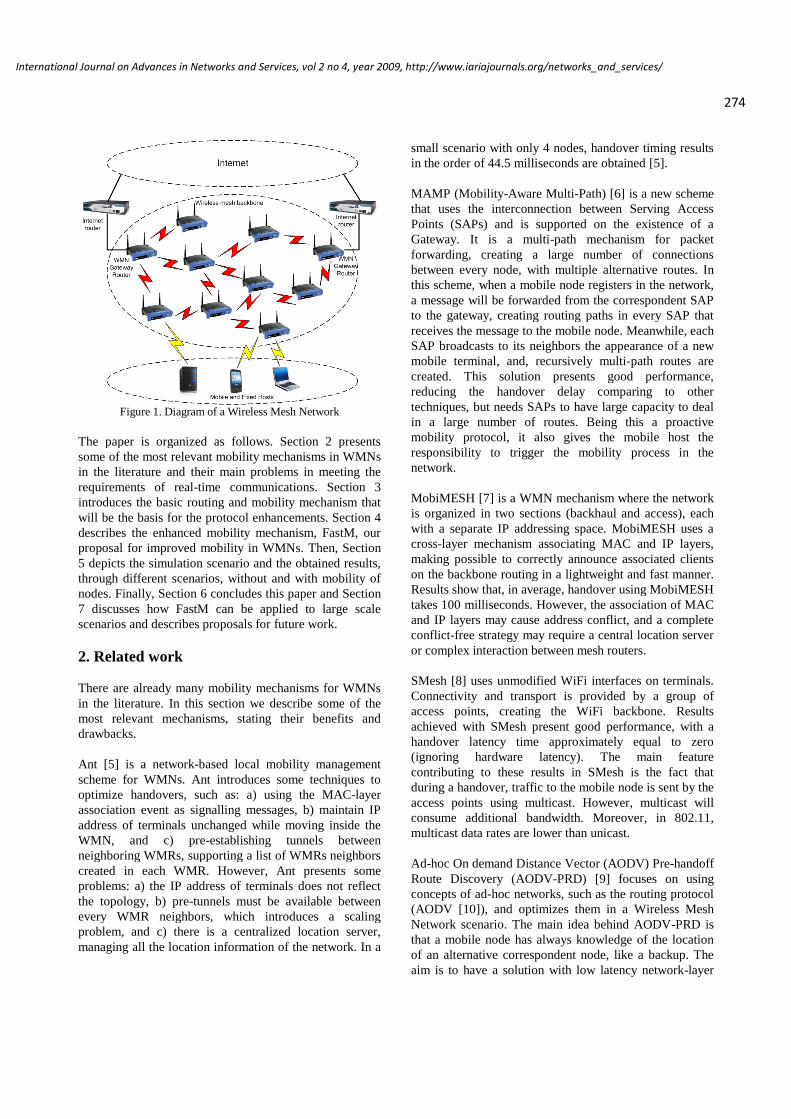
handovers and with low overhead, reducing routingdiscovery process when movement occurs. When a mobilenode detects that the SNR value of the currentcorrespondent node falls below a given threshold, itinitiates a link-layer scan to detect neighbor wireless meshrouters. From this list, the mobile node selects the wirelessmesh router which was detected with the highest SNRvalue, as its new correspondent node in the handoverprocess. At this time, AODV-PRD is integrated with thesignaling scheme of Fast Mobile IPv6 (FMIP) [11] byextending the Fast Binding Update and Handover Initiatesignalling messages with a pre-handoff route discoveryrequest option. This mechanism follows the intention ofhaving mobility mechanism free of changes in thehardware of wireless mesh nodes; however, it also suffersthe problem of the adaptation to a wireless mesh networkscenario.
QMesh [12] uses a different concept from the one thatgave birth to wireless mesh networks. This solutionassumes the existence of several gateways, and QMeshuses a common practice to always assign a user to thenearest gateway. When a user moves and associates with anew correspondent node that is closer to a differentgateway than its current one, it automatically performs ahandover between gateways. This solution is purelylocation-based, application-transparent, and does not incura high performance impact, promoting an efficientgateway assignment. One of the main points that QMeshsecures is the Quality of Service (QoS) in the mobilitymanagement solution. Parameters that incur QoSdegradation and additional costs, e.g., network distancesand congestion, server (gateway) loads, an optimizedgateway assignment algorithm must be taken into account.QMesh has two types of different decisions to manage,one regarding QoS and other regarding mobilitymanagement in the wireless mesh network. Mobile nodescan then choose between: migrate between two gateways,and choose a gateway upon a transition. QMesh performsa trade-off between assigning the user to the gateway thatprovides the best QoS at any given time, and reducing thenumber of costly gateway handovers. However, it has tobe evaluated the costs involved in the monitoring of theQoS parameters, congestion and loads, and if theycompensate not to assign a user at its nearest gateway. Tomanage this solution, some tables need to be created inevery router. QMesh maintains two main data structures ineach mesh router: a LUC (Local User Cache), which holdsthe MAC addresses of the mobile nodes whose 802.11beacons are received by the mesh router, and a GUC(Global User Cache), which holds the mapping of theMAC addresses of the mobile nodes that this node isaware, through the APs that it can be reached at. There isa balanced decision between what is best for the handoverprocess and what is best in terms of QoS.
Geo-mobility [13][14] is an approach that adopts ageographical solution for mobility and locationmanagement in spontaneous wireless mesh networks. Likemost of the solutions based on locations points, this oneneeds that nodes know exact geographical positions, bymeans of GPS or similar, while other nodes can estimatetheir relative positions. With all this data, it is possible tocreate a global topologically consistent addressing space.The resulting addressing space is pseudo-geographical, inthe sense that the coordinate space is virtual and relative,but anchored in the real world through the exactgeographical positions of some routers. Then, an End-Point-Identifier (EID) is used in every mobile node. TheEID is a value adopted by the mobile node that remainsthe same while the mobile node moves around in thewireless mesh network. At a given location, the mobilenode uses the address of a nearby router to becomereachable from any other location in the WMN. As othersolutions, Geo-mobility needs to have some type oflocation service, where the correspondence of each mobilenode between its EID and its current address is made. Thelocation service, being distributed and scalable, iscomposed by several hash functions giving the robustnessneeded. Virtual Home Region [15] is a concept adapted tothe location service, with the necessary modifications inorder to fully adapt to a wireless mesh scenario. The mainpoint that turns this solution adapted to several situations,is the flexibility that is offered based on the movement ofa mobile node. If a node moves in short distances, theaddresses of nearby routers are topologically close to eachother (geographical addressing), and updating addressescan be done in a lazy way (low signaling overhead). Thehandover performance depends on the update rate of thelocation service (which intrinsically is involved with theaddressing update), and it is assumed that a mobile nodemoves between closer mesh routers. Re-routingmechanism is performed during the handover through theshortest path. The drawback of this solution is that thenon-standard-IP addressing mechanism used can introducemore overhead in the global-state-routing update.
Some other solutions, like Wireless mesh MobilityManagement (WMM) [16] try to combine optimizationfor mobility management and for routing mechanism.Using IEEE 802.11 as the link-layer handover procedures,WMM creates in every wireless mesh router a sort oflocation service while routing data packets. The locationcache brings efficiency to routing packets with mobility ofnodes. Every mobile node has a correspondent router; inWMM it is called Serving Mesh Access-Point (SMAP). Itis the SMAP that manages all the location information ofthe mobile nodes assigned and in its radius. Whenmobility occurs, the SMAP is updated by the locationmanagement, combined with a re-forwarding technique of
275
International Journal on Advances in Networks and Services, vol 2 no 4, year 2009, http://www.iariajournals.org/networks_and_services/
data packets, using the old and new SMAP in the dataflow. Two different cache tables are used to support theseprocedures, one for routing and other for location. InWMM they are called the routing and proxy table. Thefirst manages the routing paths in the wireless meshnetwork; the second manages the location information ofmobile nodes. Using both tables makes WMM morerobust and functional in a dynamically network. Everyrouter has detailed information about the mobile nodespresent in the network. One disadvantage of this solutionis the overhead and signaling that exists inside the WMN.In large networks, the mesh routes are very solicited,needing to have high performance standards to respond toall solicitations and route correctly in the network.
Finally, although IEEE 802.11r [17] is able to provide fasthandover between stations, it is not able to handle the L3recovery of the network, in terms of routing paths andneighbor information, in order to reduce the latency on theupdate of the new path in the overall network. Ourproposed mechanism will be able to work both withunmodified IEEE 802.11 and IEEE 802.11r, since ourapproach is performed at the IP layer.
3. MeshDV and EMM
In this section we present two mobility mechanisms inlarger detail, MeshDV [3] and Enhanced MobilityManagement (EMM) [4], as they will be the basis of ourproposal, FastM.
A. MeshDVMeshDV is a solution proposed for WMNs based onequipments composed by two wireless interfaces, eachdedicated to a different sub-network: one offeringconnectivity to end-user terminals; the other forming aself-organized wireless backbone. The client interface isconfigured as an access point, while the interface used tomaintain the wireless backbone, the mesh interface, isconfigured in ad-hoc mode. These two sub-networks willhave different routing and addressing mechanismsoperating on them. Highly adaptable routing solutions arerequired in the transport sub-network enabling WMR toroute traffic from and to terminals. For this task, it wasproposed a routing solution based on the Destination-Sequenced Distance Vector (DSDV) routing protocol [18]running in IPv6. Clients only need to maintain informationabout their current point of attachment to the network.Traffic is sent towards each correspondent WMR and nomodification to the routing protocol is required at theterminals.
Each WMR has a Local and a Foreign Client tables (LCand FC) that keep track of clients present in the network:
the LC table contains the list of clients directly assigned tothe WMR; the FC table contains the information aboutclients and their correspondent WMR, which is requiredin order to allow communication between these nodes andthe local ones. MeshDV uses a tunnel-based approachcreating a communication channel between end terminals.Terminals only need to know the IP address of thedestination client and query the current WMR (usingAddress Resolution Protocol - ARP - or IPv6 NeighborDiscovery mechanisms). When the client queries theWMR for the location of a given node, the WMR willsearch its LC table. If the node is not local, it then queriesother WMRs in the network and adds this information tothe FC table. The client only needs to send packets to itscorrespondent WMR. The WMR will then create a tunnelfor the communication with the correspondent WMR ofthe destination client.
The module making all this process transparent makes useof the Neighbor Discovery Protocol (NDP) [19], which isubiquitous in all systems. This way, clients do not needany additional mechanism to communicate, makingpossible the integration of off-the-shelf equipment withoutmodifications. Traditionally, nodes use NDP to maintaintrack of the local neighbors and check their localreachability. NDP uses a set of packets and caches toshare and maintain information related to nodes in anetwork. Using MeshDV, the protocol will alter theoperation of NDP (at the WMR), allowing impersonationof the remote terminals.
MeshDV introduces several additional messages in orderto manage communication, association, and disassociationevents. These messages only exist in the backhaul part ofthe network and are mostly related to the discovery andadvertisement of clients:
MCREQ – Multicast Client REQuest – This type ofmessage is sent by a WMR when the location of aclient in the wireless mesh network is unknown.
UCREQ – Unicast Client REQuest – This is a periodicmessage that is generated by the WMR to check if theinformation present in the FC table regarding aparticular client is still valid. The purpose is to confirmif reachability still exists.
CRREP – Client Request REPly – When a WMRreceives a MCREQ or a UCREQ and if the client isconnected (present and active in the LC table), theWMR answers with this type of message with therequested information.
CWIT – Client WIThdraw – When a client disassociatesfrom a WMR, this message is sent to all the WMRsthat requested information about this node, effectively
276
International Journal on Advances in Networks and Services, vol 2 no 4, year 2009, http://www.iariajournals.org/networks_and_services/
notifying them of the withdraw event. Upon receivingthis message, a WMR will update his FC table.
- CWREP – Client Withdraw REPly – When a WMRreceives a CWIT message and has an entry with the clientaddress in the FC table, it sends a CWREP packet to theWMR that issued the CWIT announcing that the entry wasdeleted from the table.
In MeshDV, mobility management is based on feedbackfrom the wireless card (MAC layer) and periodicmessages (IP Layer). The problem with this approach isthat it is affected by the beacon timeout configuration ofthe wireless driver. When timeouts are considerably long,it is possible that (incorrect) information regarding somenode is kept in a WMR for a long time, resulting inconnectivity problems. WMRs, as defined by MeshDV,are responsible for all tasks of the handover process,communicating with the other WMRs in order to updatecaches and maintain information coherent. Standardversions of MeshDV use an approach of self-detection (apredictive approach) where a mobility manager module isresponsible for managing the handover process. Whilebeing a valid approach, it has poor performance in the realworld. This is more noticeable with activecommunications because, while the association of a clientwith a new WMR is a fast process, packets will still bedelivered to the old location for some time. The result ishigh packet loss during the handover period until cachesexpire (a few seconds). This process must be performed ina completely transparent manner to the terminals andconsuming the minimum bandwidth. Also, handover mustbe a fast process with minimal packet loss, givingterminals the possibility of maintaining activecommunications across different attachment points.
B. EMMEnhanced Mobility Management (EMM) [4] is a newoptimization to MeshDV, designed to improve mobilitymanagement, and reduce handover delay. With thissolution, a new reactive approach for mobilitymanagement is proposed, with the detection of the clientsduring their movement performed by the new WMR. Thissolves the refresh delay problem created by the NDPcache [19]. Results show that EMM [4] reduces thehandover latency time in MeshDV Network, in somecases from 3 minutes to only a few seconds or less thanone second. The main change that EMM adds to MeshDVis a new type of message that is sent when a client changesits WMR association. EMM also proposes modificationsto some of the original messages and mechanisms firstproposed in MeshDV. Figure 2 depicts de EMM messagesequence diagram of a handover process.
Figure 2. Communication diagram of EMM
One of the messages added is the Unsolicited NeighborAdvertisement (UNA), which is sent by a node to informits neighbors that its link-layer address has changed,correctly updating the NDP cache of its neighbors with theMAC address of the new WMR. EMM adds an importantfeature to WMRs: when movement occurs, the old and thenew WMRs exchange information related with the oldassociation of the client. This way, the new WMR willreceive from the clients the address of the WMR wherethey were associated (via NDP) and update with its ownaddress (UNA message). Meanwhile, the new WMRinforms the old WMR of the association context related toa client. Also, the old WMR will be instantly notifiedabout the new location of its former client and clean localcaches.
When a WMR receives traffic from one of its clients witha destination MAC address different than its MACaddress, the packet is not discarded. Instead, the packet istunneled and forwarded to the proper WMR serving thedestination address. Then, the WMR sends an UNAmessage to the client in order to update its NDP cachewith the value corresponding to the MAC address of theWMR.
Another message that is added to the MeshDV system isthe Client Error message (CERR), which is sent by thedestination WMR directly to the source WMR, informingthat the client is not associated with it anymore. Receivinga data packet to a node that was removed from the LCtable triggers this message.
EMM corrects most of the issues affecting the originalMeshDV proposal aiming to be adaptable to wirelessmesh networks in general. Results in [4] show reduceddisconnection times by a large factor. However, EMM still
277
International Journal on Advances in Networks and Services, vol 2 no 4, year 2009, http://www.iariajournals.org/networks_and_services/
achieves results in the order of seconds, thus it is unableto support voice continuity in wireless mesh networks.The problem is that data packets in transit during themobility process are dropped by the WMR previouslyused by the client. Another issue is the existence of a largecontrol overhead sent to the network when mobilityoccurs. The existence of multicast packets during themobility process for the WMR to be able to locate thesender and receiver client after a handover, creates a largenumber of unnecessary packets, floods the network andincreases the time of the process to locate nodes in thenetwork. Solutions to provide mobility in WMNs must beable to offer better performance with respect to adapt tothe actual requirements of nodes, and at the same time, beeasy to deploy in real networks. Even being a valid andimportant improvement, EMM is still not able to supportreal-time communication during the handover process.
4. FastM: Fast Mobility Support extension
FastM was developed to further optimize mobility inWMNs. It is an evolution of EMM and MeshDV,inheriting the basic functional aspects, but modifying keyfunctionalities, and adding a significant set of effectivefeatures. As MeshDV, FastM uses both local and foreigntables, and proposes a new table named Neighbor Clienttable (NC) used to keep information about neighbornodes. With the addition of this table, which effectivelyexploits locality, a new set of control messages is used inorder to maintain the coherence of the mesh network.These changes aim to avoid packet loss for the duration ofthe handover process, reduce control multicast packets inthe network, save bandwidth and optimize the associationand disassociation processes of clients to WMRs. Theresult is a much optimized and effective solutionproviding services like voice continuity over WMNs.
With the neighbor table, all updates made to the local andforeign tables in any WMR are broadcasted to all itsneighbors (TTL=1). From real experiments, we notice thathandovers are typically performed to neighbor WMRs. Inthis case, when a data packet reaches an old WMR, theaddress will be found in the neighbor table and the WMRautomatically re-tunnels the packet towards the newlocation of the client, avoiding packet loss. This producesextremely fewer Client Request packets and speeds thehandover process. Our solution does not try to maintaintables consistent, and we assume some incoherence mayoccur. Nevertheless, if a node has inconsistentinformation, the algorithm will resort to standard nodelocation mechanisms, guaranteeing proper operation.
A. Signalling ApproachFastM uses a new set of messages to improve the mobilityprocess: CLIENT_IS_THERE – When a WMR receives data
packets to a client that is in its neighbor table, theWMR checks its foreign table, and a message is sent tothe WMRs that had communication with that client.This message contains the new location of the client,enabling FastM to also support mobility that involvesother WMRs besides the direct neighbors.
CLIENT_IS_THERE_CONF – By receiving aCLIENT_IS_THERE message, the WMR is notifiedthat a node moved. Then, this WMR sends to theWMR at the new location, a confirmation stating that aclient attached to the first one is communicating with aclient attached to the second one. This message acts asa confirmation to the handover process.
TABLE_UPDATE – This message is broadcasted toneighbors (TTL=1) when the Client table changes.Updates like associations, disassociations, andhandovers are then known by every WMR in theneighborhood.
TABLE_UPDATE_HELLO – In order to periodicallyrefresh node status, and every 30 seconds, all WMRssend a TABLE_UPDATE_HELLO announcing thatthey are still alive, and that no changes had occurred tothe Client table.
Figure 3. Communication diagram of FastM
Figure 3 depicts the communication diagram of ahandover. The changes that characterize this procedureare immediately noticed: there is a tunnel between old andnew WMRs, which enables packets to reach theirdestination until the protocol finally converges; also, nomulticast packets are sent to locate clients in the network,in the case of location information is present in theneighbor table. The process occurs as follows:1) Client 1 issues an ASSOCIATION_REQUEST
message to a new WMR. This is a standard 802.11message. Scanning delays with the new association in
278
International Journal on Advances in Networks and Services, vol 2 no 4, year 2009, http://www.iariajournals.org/networks_and_services/
IEEE 802.11 are out of scope of our work. Theproblem of loosing performance with scanning delayscan be resolved using solutions like the one describedin [20].
2) The new WMR accepts the association and sends anASSOCIATION_REPLY message (also standard802.11) to Client 1. Because the Client table isupdated, it broadcasts a TABLE_UPDATE messageto all neighbors WMR notifying others about thetopology change.
3) When the correspondent WMR forwards packets fromClient 2 to Client1, their destination is the old WMRbecause the correspondent WMR is not informed ofthe handover process. Data packets arriving to the oldWMR are re-tunneled to the new WMR, thus no lossoccurs only delay is added. The old WMR will thensend a CLIENT_IS_THERE message to thecorrespondent WMR notifying it that Client 1 has leftto the new WMR.
4) Correspondent WMR answers to the new WMR with aCLIENT_IS_THERE_CONF message. This confirmsthe new location and informs the new WMR aboutthe location of clients that were communicating withthe Client 1.
Basically, these are the steps that FastM makes in order tocomplete a handover process. We can see that in thisprocess the signaling required to perform the handover ismainly between neighbor nodes, which decreases thehandover latency and control overhead. There are alsochanges in the Client Table of each WMR in order tostore location information thus predicting futurehandovers and facilitating them.
B. Example of FastM OperationFigure 4 uses an example to show the several steps toreach a successful handover with the FastM mechanism,and to better introduce the changes to the several tables inthe handover process. These tables are used to manageneighbor handovers with low latency and without errors.
In Figure 4, in step 1, it is shown the communicationbetween node 1 and 6, and the 3 client tables, local,foreign and neighbor, of the mesh nodes 2 to 5. Forexample, in step 1, where client 1 is transferring UDPtraffic with client 6, node 3 contains: node 1 in its localclient table, which is the node directly connected to it;node 6 in its foreign client table (64, means that node 6is connected to node 4), which is the node in the meshnetwork but not connected to it; and no information in itsneighbor client table, since it has no knowledge aboutneighbors with communication. Node 2 contains noinformation in local and foreign tables, since this node
does not have active communications. However, node 2has information in its neighbor table of node 1, which isconnected to node 3. Since the information in 3 comesfrom the local table, the third number is 1 (131).Notice that this third number does not address a specificnode, but informs if the information came from a local (1)or a foreign (2) table. Node 2 also contains information inthe neighbor table about node 6 that is connected to 4 andwhose information came from the foreign table of node 3,and therefore, the third number is 2 (642). Node 4 isthe same case as node 3 in terms of the neighbor table,and contains node 6 in its local table (the node it iscommunicating with). Finally, node 5 has no informationon local and foreign tables, similarly to node 2, andcontains node 6 in its neighbor table, which is connectedto node 4 and whose information came from the localtable of node 4 (and therefore the third number is 1:641).
When node 6 moves, it sends an association message tonode 5, which will contain now node 6 in its local table(step 2). Then, in step 3, node 5 announces node 4(neighbor node) that node 6 is performing handover; nownode 6 is in the foreign table of node 4 (obtained throughnode 5), and the neighbor table contains node 6,connected to node 5 and whose information came from thelocal table of node 4. Then, in step 4, the node 4 forwardsthe data packets in transit to the new location; it alsoannounces to node 3 the location of node 6. Node 3updates its foreign table with node 6 connected to node 5.Node 3 then sends information of the new location of thenode to the old path of the communication flow, whichtriggers an update of the neighbor table of node 2, whichnow contains information from node 5 (step 5). At thisstage, all nodes in both new and old communication pathshave information on the handover of node 6, and thennode 5 confirms to node 4, the previous node associatedto node 6, that the handover process is terminated. Node 4updates its neighbor table with information of node 1connected to 3, and it will finish the process of forwardingdata packets (step 6). Finally, the handover process isfinished and the packets are forwarded through the newpath (step 7).
279
International Journal on Advances in Networks and Services, vol 2 no 4, year 2009, http://www.iariajournals.org/networks_and_services/

Figure 4. Steps in the handover mechanism of FastM
5. Simulation results
The solution described above was implemented and testedusing the ns-2 simulator, version 2.31 [20] on an UbuntuLinux environment.
Two different scenarios were evaluated: one to compareFastM enhanced MeshDV (MeshDV FMS) with standardMeshDV, and one to provide a more detailed study of theMeshDV with FastM solution in mobile environmentswith increased mobility. Evaluation of FastM MeshDV incomparison to EMM MeshDV will be addressed in futurework.
In order to compare the FastM solution with standardMeshDV, a cloud-type scenario has been chosen with 37nodes, in a square flat area of 6400 m2 (800m x 800m).The number of nodes and the topology was chosen toenable the change of several paths during the handover.The MAC layer protocol is the IEEE 802.11 with 11Mbps of maximum bandwidth, and 150 m of transmissionrange for every node. This scenario is depicted in Figure5.
280
International Journal on Advances in Networks and Services, vol 2 no 4, year 2009, http://www.iariajournals.org/networks_and_services/
Figure 5. Simulations scenario: comparison between MeshDVand FastM
UDP and TCP flows are generated between two clientsnodes as shown in Table 1. In all simulations the receivernode performs handover at t=270 seconds, while thesender node switches attachment point at t=370 seconds.Total simulation time is 450 sec.
Table1. Characteristics of the scenariosConfiguration 1 Configuration 2
Traffic type UDP CBR TCP
Packets size 84 bytes 1060 bytesSending rate 100 pkt/sec N/A
Number of flows 1 1
In order to better mimic the real world, artificial delayshave been introduced in the WMN. These delays are usedto emulate the delay required for the network interface tochange channel and the network stack to configure a newaddress (50 milliseconds). The value is derived fromprevious work performed [22]. Other relevant aspect is theartificial control delays implemented in ns-2 toapproximate even more the simulations to real situations,in what refers to the implementation of MeshDV, both inEMM and FastM. All other values are set to their defaults.Control packets are retransmitted if an answer (or action)is expected and was not detected, with a backoff startingat 1s.Using this simulation environment, we evaluate MeshDVwithout and with FastM, according to the followingmetrics: throughput, packet loss and control overhead.
Figure 6. Throughput of MeshDV in the static case and in case ofhandover (receiver at t=270s, sender at t=370s).
Figure 7. Throughtput of MeshDV with FastM in the static caseand in case of handover (receiver at t=270s, sender at t=370s).
Figure 8. Throughput comparison of MeshDV with and withoutFastM. The later shows little interruption.
A. ThroughputAs depicted in Figures 6, 7 and 8, the results obtainedduring the handover process, without and with FastMextension, for both configurations, are quite different.The first curves describe throughput when no handoverhas occurred. In this situation, and for all cases,throughput is stable. When the receiver changes its pointof attachment (second curves), throughput may take sometime to reach its previous values if MeshDV is used.
281
International Journal on Advances in Networks and Services, vol 2 no 4, year 2009, http://www.iariajournals.org/networks_and_services/
FastM shows a rapid recovery. If the sender moves (lastcurve), disruption occurs again and can last for severaltens of seconds (using MeshDV). Table 2 compares thesedisconnection delays with physical testbed results,obtained with MeshDV and EMM and previouslypresented by its authors in [4].The testbed experimental results of both MeshDV andEMM (Table 2) show handover times in the orders ofseconds; even in EMM (which is the best case) thehandovers when using UDP sessions require 2 to 4 sec,while the ones of TCP sessions require 35 to 40 sec. Insimulations, the values are considerably lower. However,TCP sessions in MeshDV induce disconnection delays inthe order of 60s, which is unacceptable for normalcommunications (even if not real-time). This happens dueto inappropriate scanning process, sub-optimal NDPcache handling, and 802.11 scanning. TCP performs worstthan UDP due to the rate adaptation algorithm, whichtakes a long time to recover when packets are being lost.
Table 2. Disconnection time comparisonReceiver Handover(s)
Sender Handover(s)
UDP TCP UDP TCPMeshDV1) 15 240 190 185EMM1) 2 40 4 35
ns-2MeshDV2)
0.279 61.287 0.340 59.537
ns-2MeshDV2)3)4)
0.279+[0...180]
61.287+[0...180]+[0...30]
0.340+[0...180]+[0...30]
59.537+[0...180]+[0...30]
ns-2FastM2)4) 0.118 0.344 0.089 0.141
1) Results obtained on a physical testbed (see [4])2) Results obtained through simulation in ns-23) The wireless driver used by the AP’s in the physical testbed, has ascanning delay, which varies between 0 and 180 seconds, and increaseshandover time by ~90s.4) Due to the use of NDP in clients, there’s a cache update delay, whichranges between 0 and 30 seconds. This will increase handover time by~15s.(Inclusion of notes 3) and 4) aims at providing results closer to the onesexpected in real world scenarios)
Comparing the disconnection times in Table 2 betweenMeshDV and FastM (through simulation), the valuesobtained in FastM are significantly lower. With UDP,even when both sender and receiver clients move, trafficvalues are reduced and the timeout imposed by thewireless driver and NDP are suppressed; in this case, thehandover time is reduced from 300 milliseconds to 100milliseconds, a 3 times improvement. Using TCP traffic,the differences are even more evident: the techniquesimplemented in FastM (which minimize packet loss) areable to lower the disconnection time to milliseconds(between 100 and 300 milliseconds) compared to the 60seconds of MeshDV (an improvement of more than 200
times). This large disconnection delay happens due toTCP congestion avoidance mechanism. Whendisconnection occurs, and both delay and loss figuresincrease, TCP will reduce the packet rate in order tominimize loss. Because disconnection time spans forseveral seconds, the exponential backoff will increase tohigh values, further increasing disconnection time for TCPapplications. Ultimately, sessions may be terminated andthen restarted. When using FastM, because disconnectiontime takes only a few hundreds of milliseconds, backoffnever reaches high values, and TCP recovers morerapidly. Moreover, TCP creates two flows requiringrouting, which greatly increases disconnection time.
B. Dropped PacketsFigure 9 shows the amount of dropped data packets inevery scenario. The results using FastM in MeshDV showa large decrease of dropped packets during handovers,both in UDP and TCP traffic.
Using UDP traffic this difference is more noticeable dueto a 10 seconds gap in which the communication betweenthe clients is non existing due to NDP session timeout (asthe handover occurs at t=370s, it only needs 10 secondsfor the NDP timeout, since it is issued every 30 s). In thisperiod, there is a large number of dropped packets, as thesession in the client is not updated to the address of thenew WMR. When the receiver handover takes place(t=270s), there is a small number of dropped packets,during the period the receiver changes attachment point,and the new WMR searches the location of thecorrespondent client (sender node).
With respect to FastM, there are no dropped packets whenthe receiver changes attachment to a new WMR. This isdue to the re-tunnel of data packets in transit. When theserver handovers to a new WMR, some packets are lostduring the time it takes to disassociate and associate to anew WMR. An improvement of 97.3% (from 546 to 15packets) is obtained with the use of FastM in MeshDV.Using TCP, FastM also shows great improvements, in thiscase of 35.1% (from 57 to 31 packets). As it can be shownin Figure 10, there are fewer packets generated whenFastM is not used in MeshDV, which will also result inless packets being dropped. This happens because thelocation of clients is unknown after handovers. WithFastM, packet generation is constant and some losses existdue to the TCP characteristics, such as drop links and fullqueues, during the simulation period. During handover,only 7 packets are dropped (4 in the first, 3 in the secondhandover) between the disassociation and associationtimes of clients to a new WMR.
282
International Journal on Advances in Networks and Services, vol 2 no 4, year 2009, http://www.iariajournals.org/networks_and_services/
Figure 9. Sum of dropped packets after stabilization
Figure 10. Comparison between generated and drops packets
C. Control MessagesIn what refers to control messages (Figure 11), there aresignificant changes using MeshDV with and withoutFastM. While analyzing the performance of MeshDVwithout FastM, we see a typical and coherent laddershaped process during the simulation. This is presenteither using UDP or TCP traffic. The initial controlpackets (t=10s) are due to the initial associations of theclients to the WMRs. At t=140s, when data transfer starts,some control packets are generated in order to locate thecorrespondent clients in the WMN. With TCP traffic,there are two client location processes (the second takesplace at approximately t=143s), due to the packet flows ofTCP (data and ack). Then, in each handover, controlpackets are generated in order to locate the clients. InTCP, due to the loss of links, some exchanges of packetsare performed after the handover takes place, causing adisconnection time during this period.
Figure 11. Sum of control packets sent to the network.
Using FastM extension in MeshDV, when mobility takesplace, the number of control packets is reduced. Due tothe existence of the neighbor client table, there areTABLE_UPDATE_HELLO messages every 30 seconds.During the handover, FastM reduces the control packetsfrom 117 packets to 112 packets in UDP traffic, and from226 packets to 152 packets in TCP traffic. With thistraffic, an improvement of 32.7% in control packets isobtained. This will be even more significant in a scenariowith larger number of mobile nodes and more frequenthandovers. Please consider that the improvement weachieve is expressed in terms of number of packets sent tothe network, which is more appropriate considering thatthe medium is shared. A single message sent by a nodewill lead to the generation of multiple packets (one foreach forwarding node, plus one sent by the origin). Bybetter exploring locality, from one side communicationsare reduced, and from the other they involve nodes incloser proximity, thus reducing the impact of the routingprotocol.
D. Mobility SpeedIn this section we analyse the performance of the FastMsolution with respect to the speed of the mobile client. Thescenario is similar to the previous one, but nodes areplaced on a square grid instead of a circle, as shown inFigure 12. This square scenario was used in order tosimplify the mobility pattern and the estimation of theposition (and point of attachment) of the mobile node. AllWMR nodes are fixed, while one mobile node movesaround the others at speeds ranging from 4m/s to 16m/s.This node (node 26), starts its movement at the lower leftcorner, and moves first to the right, then up, left anddown, stopping near to node 2. In this scenario, the mobilenode is communicating with one of the fixed nodes eitherusing TCP or UDP. When using TCP, it sends packetswith 1000 bytes of data (1040 bytes including TCP and IPheaders); bandwidth is limited only by TCP internal
283
International Journal on Advances in Networks and Services, vol 2 no 4, year 2009, http://www.iariajournals.org/networks_and_services/

contention mechanisms. When using UDP, the node sendsa CBR flow with packets of 1000 bytes and a constantperiodicity of 10 milliseconds. As in the previous case,total simulation time is 500s and the flows start at t=100s.
Figure 12. Simulations scenario: FastM with increased mobility
Concerning delivery rate in Figure 13, we observe that thetotal number of packets received decreases with theincrease of velocity. These results are inline with ourexpectations and reflect the proper operation of therouting protocol and handover approach in the meshnetwork: mobility decreases the time between handovers,and with more frequent handovers, the losses areincreased, which consequently decreases the throughput.One interesting aspect is that delivery rate seems todecrease more rapidly at lower speeds, reachingstabilization at higher speeds. Above 10 m/sec, resultsshow that the protocol is able to maintain some minimaldelivery rates. This shows the effectiveness of theneighboring tables: with higher handover frequency, thereis less time for tables to be disseminated and normalMeshDV handover process occurs (the effect andenhancement of FastM is minimized). More aggressivetable maintenance strategies could help increasing theperformance; still, the resulting higher overhead wouldprobably nullify the overall performance improvement. Asexpected, UDP achieves higher delivery rate than TCPdue to the inexistent flow control mechanisms in UDP;however, the trend is similar to both types ofcommunications.
Figure 13. Comparison between throughput in FastM in TCP andUDP as a function of mobile node velocity
According to the results presented in Figure 13, we wouldexpect that overhead would be higher when neighbortables are being maintained (more maintenance in smallmobility scenarios), and this is shown in Figure 14. Thisgraphic depicts the number of control packets sent to thenetwork as a function of speed of the mobile node. Forlower mobility, as nodes slowly hop between the WMRs,neighbor tables are filled and propagated to theirneighbors, thus producing a higher overhead. As the nodesstart to move with a higher speed (and we realize from thegraphic that the critical point is at 10 m/s), the neighborclient tables construction becomes more inefficient, sincethere is less time to propagate the tables to the neighbors,and this reduces total overhead.
Related to the difference between UDP and TCP curves,TCP has, in most of the cases, increased overhead, as inthe first scenario depicted in Figure 11. For increasedspeed, the difference in overhead is not so noticeable: thisis due to the mobility effects on TCP sessions.
Figure 14. Number of control packets sent to the network as afunction of node velocity
284
International Journal on Advances in Networks and Services, vol 2 no 4, year 2009, http://www.iariajournals.org/networks_and_services/
6. Conclusions
The support for VoIP applications in current and futureWMNs is considered to be vital to its success. However,the wireless medium and multi-hop routing protocols arefrequently unable to meet the requirements of seamlessmobile nodes handover, while maintaining uninterruptedcalls: efficient mobility mechanisms are required toenhance the performance of the communications in thesenetworks in mobile scenarios.
In this paper, we proposed a novel extension to improvethe mobility process, denoted as FastM, that integratesmobility and routing mechanisms, and that brings a newway to deal with neighborhoods, using other nodes tomaintain information about the organization of the WMN.Results obtained with ns-2 prove the efficiency of thesolution and its effectiveness in meeting the requirementsof low packet loss, disconnection times, and controloverhead, even in scenarios with increased mobility. Thedisconnection times were reduced to values around 100milliseconds, being able to meet the real-timecommunications requirements.
7. Future Work
This mobility mechanism is based in principles that aretransversal to other mobility mechanisms that existnowadays. In this paper this solution was applied toMeshDV; however, its concepts are applicable to mostproactive routing protocols. Its support in EMM will beaddressed as future work.
New routing processes use concepts related to k-neighborhoods where the algorithm itself organizes thenetwork in several groups, having a number of nodes witha global perspective of the overall network, one for eachgroup. Adapting this concept to the principle behindFastM is intuitive. FastM is supposed to be a mobilitymanagement in small perspective, using the relationsbetween neighbors to re-forward packets and adjust thetopology when mobility occurs. This way, implementingFastM inside every neighborhood to support micromobility management and in every group leader to supportmacro mobility management, it will be created a systemwith fully support of micro and macro mobilitymanagement integration with considerably gains. Thisintegration brings two main advantages: larger routingcapacity in large networks and capacity of maintaining k-neighborhoods with high performance. FastM contributeswith good results on handovers: no packet loss, lowtimeout and high performance on route convergence.These two techniques combined add a great robustness toa network when handovers occur. Applying the
procedures in very large networks will have no influencein the global performance, as the responsibilities andoverloads are distributed between all the k-neighborhoods.
Other future work in this area also concerns theimplementation of the mobility approach and thecomparison of simulation and experimental results, toassess the behaviour of these mechanisms in realenvironments. Moreover, a comparison should be madewith different mobility solutions.
AcknowledgmentsThis work was partially supported by the EuropeanCommission project IST-WIP under contract 27402.
8. References
[1] L. Couto, J. P. Barraca, S. Sargento, R. L. Aguiar, “FastMin WMN: a Fast Mobility Support extension for Wireless MeshNetworks”, The Second International Conference on Advancesin Mesh Networks (MESH 2009), Athens (Greece), June 2009.[2] IST WIP – An All Wireless Mobile Network Architecture,http://www.ist-wip.org.[3] L. Iannone and S. Fdida, “Meshdv: A distance vectormobility-tolerant routing protocol for wireless mesh networks”,IEEE ICPS Workshop on Multi-hop Ad hoc Networks: fromtheory to reality (RealMAN’06), July 2005.[4] M. Bezahaf, L. Iannone and S. Fdida, “Enhanced MobilityManagement in Wireless Mesh Networks”, Journées Doctoralesem Informatique et Réseaux (JDIR08), January 2008.[5] H. Wang, Q. Huang, Y. Xia, Y. WU, Y. Yuan, “ANetwork-Based Local Mobility Management Scheme forWireless Mesh Networks”, In Proc. of WCNC 2007.[6] Y. Fan, J. Zhang, X. Shen, “Mobility-Aware Multi-PathForwarding Scheme for Wireless Mesh Networks”, In Proc. ofWCNC 2008.[7] A. Capone, M. Cesana, S. Napoli and A. Pollastro,“MobiMESH: a Complete Solution for Wireless MeshNetworking”, IEEE, 2008.[8] Y. Amir, C. Danilov, et al., “Fast Handoff for SeamlessWireless Mesh Networks”, In Proc. of MobiSys’06, June 2006.[9] S. Speicher, C. H. Cap, “Fast Layer 3 Handoffs in AODV-based IEEE 802.11 Wireless Mesh Networks,” In Proc. of 3rd
International Symposium on Wireless Communications Systems(ISWCS),Sept, 2006.[10] C. Perkins, E. Belding-Royer, S. Das, “Ad hoc On-Demand Distance Vector (AODV) Routing,” RFC 3561, 2003.[11] G. Koodli, “Fast Handovers for Mobile Ipv6,” RFC 4068,Jul., 2005.[12] E. Bortnikov, T. Kol, A. Vaisman, “QMesh: a QoS MeshNetwork with Mobility Support,” In Proc. of ACM SIGMOBILEMobile Computing and Communications, vol. 12, no. 1, Jan.,2008.[13] F. Rosseau, Y. Grunenberger, V. Untz, E. Schiller, P.Starzetz, F. Theoleyre, M. Heusse, O. Alphand and A. Duda,“An Architecture for Seamless Mobility in SpontaneousWireless Mesh Networks”. in Proc. MobiArch'07, Kyoto, Japan,August 2007.
285
International Journal on Advances in Networks and Services, vol 2 no 4, year 2009, http://www.iariajournals.org/networks_and_services/
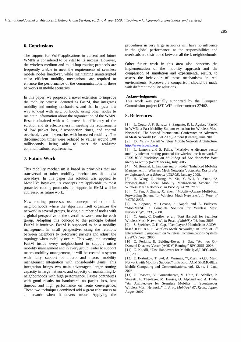
[14] F. Rousseau, F. Théoleyre, A. Duda, A. Krendzel, M.Requena-Esteso, J. Mangues-Bafalluy, “Geo-mobility andLocation Service in Spontaneous Wireless Mesh Networks,” InProc. of ICT-MobileSummit, Stockholm, Sweden, June 10-12,2008.[15] X. Wu, “VPDS: Virtual Home Region based DistributedPosition Service in Mobile Ad Hoc Networks,” In Proc. of IEEEInternational Conference on Distributed Computing Systems(ICDCS), June, 2005.[16] D.Huang, P. Lin, C. Gan, “Design and Performance Studyfor a Mobility Management Mechanism (WMM) Using LocationCache for Wireless Mesh Networks,” IEEE Transactions onMobile Computing, vol. 7, no. 5, May, 2008.[17] IEEE Standard for Information Technology-Telecommunications and Information Exchange BetweenSystems-Local and Metropolitan Area Networks-SpecificRequirements Part 11: Wireless LAN Medium Access Control(MAC) and Physical Layer (PHY) Specifications Amendment 2:Fast Basic Service Set (BSS), July 2008.[18] C.E. Perkins and P. Bhagwat, “Highly Dynamicdestination-sequenced distance vector routing (DSDV) formobile computers.” in Proc. ACM SIGCOMM 94, London, UK,Oct. 1994, pp. 234-244.[19] T. Narten, E. Nordmark, W. Simpson, “RFC 2461 –Neighbor Discovery for IP Version 6 (IPv6)”.[20] I. Ramani, S. Savage, “SyncScan: Practical Fast Handofffor 802.11 Infrastructure Networks”, Infocom 05, March 2005.[21] The ns-2 Manual (Oct. 2, 2006),http://www.isi.edu/nsnam/ns.[22] L. Couto, J. Barraca, S. Sargento, R. Aguiar, “FastMobility in proactive routing protocols”, ICT-MobileSummit 08,July 2008.
286
International Journal on Advances in Networks and Services, vol 2 no 4, year 2009, http://www.iariajournals.org/networks_and_services/
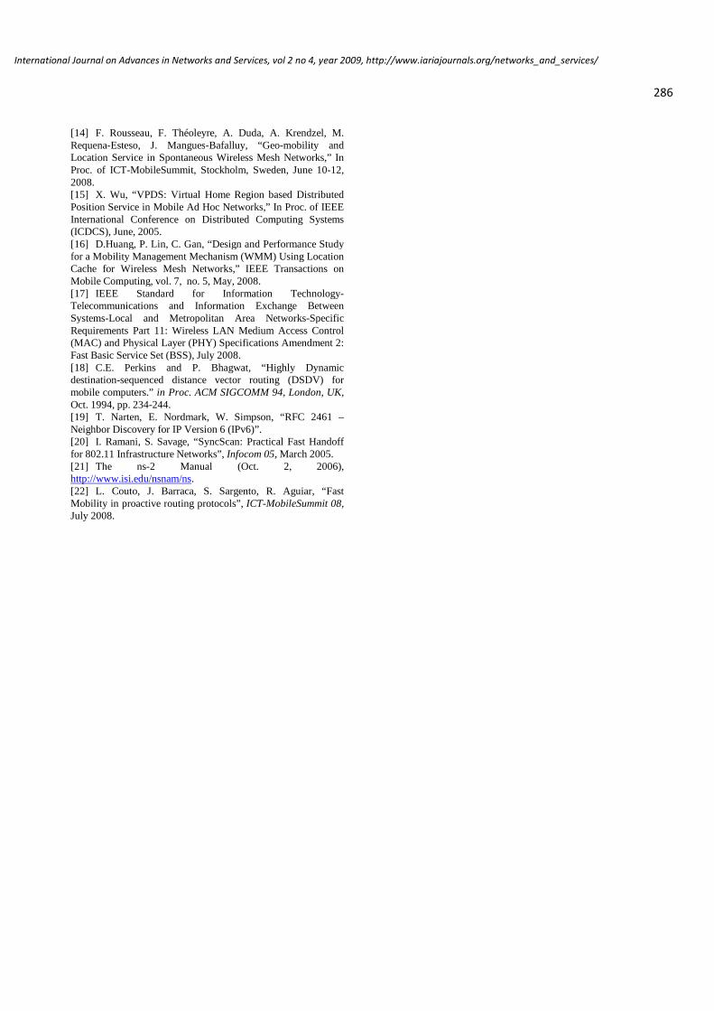
www.iariajournals.org
International Journal On Advances in Intelligent Systems
ICAS, ACHI, ICCGI, UBICOMM, ADVCOMP, CENTRIC, GEOProcessing, SEMAPRO,BIOSYSCOM, BIOINFO, BIOTECHNO, FUTURE COMPUTING, SERVICE COMPUTATION,COGNITIVE, ADAPTIVE, CONTENT, PATTERNS
issn: 1942-2679
International Journal On Advances in Internet Technology
ICDS, ICIW, CTRQ, UBICOMM, ICSNC, AFIN, INTERNET, AP2PS, EMERGING
issn: 1942-2652
International Journal On Advances in Life Sciences
eTELEMED, eKNOW, eL&mL, BIODIV, BIOENVIRONMENT, BIOGREEN, BIOSYSCOM,BIOINFO, BIOTECHNO
issn: 1942-2660
International Journal On Advances in Networks and Services
ICN, ICNS, ICIW, ICWMC, SENSORCOMM, MESH, CENTRIC, MMEDIA, SERVICECOMPUTATION
issn: 1942-2644
International Journal On Advances in Security
ICQNM, SECURWARE, MESH, DEPEND, INTERNET, CYBERLAWS
issn: 1942-2636
International Journal On Advances in Software
ICSEA, ICCGI, ADVCOMP, GEOProcessing, DBKDA, INTENSIVE, VALID, SIMUL, FUTURECOMPUTING, SERVICE COMPUTATION, COGNITIVE, ADAPTIVE, CONTENT, PATTERNS
issn: 1942-2628
International Journal On Advances in Systems and Measurements
ICQNM, ICONS, ICIMP, SENSORCOMM, CENICS, VALID, SIMUL
issn: 1942-261x
International Journal On Advances in Telecommunications
AICT, ICDT, ICWMC, ICSNC, CTRQ, SPACOMM, MMEDIA
issn: 1942-2601