international ﬁnancial transmission of the fed’s monetary

7 7

International Journal of Economic Sciences and Applied Research 7 (2): 7-49

International financial transmission of the Fed’s monetary policy

Nikola Mirkov1

Abstract

This paper proposes a way to study the transmission mechanism of the US monetary policy to foreign yield curves. It elaborates the high-frequency identification of monetary policy shocks from (Piazzesi, 2005) in an international setting. The shocks are extracted from a two-country term structure model and the procedure is illustrated on the US-UK daily data.

Keywords: term premia, Fed, policy actions

JEL Classification: E43, E52, G12

1. Introduction

Increasingly integrated financial markets are one of the key transmission channels of international macroeconomic and monetary shocks2. The transmission mechanism of the US monetary policy is particularly researched, where usually a vector autoregression (VAR) - type analysis is used to enhance our understanding of how monetary policy affects equity markets3, interest rates4 or both5. Yet, as pointed out in (Cochrane and Piazzesi, 2002), the VARs may not be sufficiently flexible to accommodate the time-varying preferences of the Fed, nor able to provide a solid identification of the Fed’s reaction to the interest rates from the interest-rate reactions to the Fed. Consequently, a high-frequency identification strategy from (Piazzesi, 2005), together with monetary policy shocks extracted from the state variables’ residuals around policy action days, can be used to analyse the impact of the US monetary policy decisions on foreign interest rates and term premia. The Fed decisions in the sample are split into two different groups, depending on the direction of the policy rate move and whether the move

1 Swiss National Bank, Borsenstrasse 15, 8022 Zurich, Switzerland, [email protected] See (Canova, 2005; Cooley and Quadrini, 2001; Ehrmann and Fratzscher, 2006).3 See (Bernanke and Kuttner, 2005; Ehrmann and Fratzscher, 2004).4 See (Taylor, 1995; Evans and Marshall, 1998; Canova, 2005).5 See (Rigobon and Sack, 2004).

Volume 7 issue 2.indd 7Volume 7 issue 2.indd 7 24/11/2014 10:32:48 πμ24/11/2014 10:32:48 πμ

8

Nikola Mirkov

was anticipated6. Different “types” of policy shocks are then used to assess the reaction of foreign yield curve to different policy actions, therefore allowing for an asymmetrical response of interest rates to policy rate decisions discussed in (Bernanke and Kuttner, 2005). The model used in the assessment is a two-country Gaussian term structure model with observable risk factors from (Joslin, Singleton and Zhu, 2011) (henceforth JSZ)7. Given the reduced-form nature of the model, the two economies are “connected” through the exchange rate between them. Following (Backus, Foresi and Telmer, 2001) and (Dong, 2006), both pricing kernels are defined and the implied depreciation rate is used to confirm that the model satisfies the widely acknowledged empirical finding8, according to which high interest rate currencies tend to appreciate, oppositely to what the Uncovered Interest Rate Parity (UIRP) would suggest. (Fama, 1984) attributes such behaviour of exchange rates to the time-varying risk premium and imposes two necessary conditions, which the proposed model satisfies. The idea of estimating the effect of US monetary policy shocks to foreign yield curves is illustrated on the UK term structure of interest rates. The two countries are close trading partners9 and their financial markets are arguably highly integrated10. The US and the UK yield curves are jointly fitted and the estimated model residuals from the days of the FOMC statements are considered as monetary policy shocks in a dynamic response of the UK yields to policy rate decisions in the US. In addition, every instantaneous change in the UK yield curve is decomposed to expected future short-rate change and the term premia change. Dynamic response of the UK yield curve to the Fed funds rate decisions is estimated to be negative, independently of weather the Fed delivered an interest rate hike or cut. The puzzling result is contrasted to the reaction of the US yields and to instantaneous changes of the UK short-rate expectations and term premia. Interestingly, both countries’ yield curves seem to steepen after expansionary policy shocks, which is broadly in line with (Evans and Marshall, 1998). On the other side, instantaneous responses of the UK yields to hikes show that the medium and long-term UK yields decline, because the implicit term premia fall11. Finally, the average estimated reaction of the UK short- and medium term premia to

6 Following the ideas in (Kuttner, 2001) and looking at the Fed funds futures market.7 The previous studies that modelled the JSZ canonical form in a multi-country setting are (Graveline and Joslin, 2011; Jotikasthira, Le and Lundblad, 2010; Bauer and de los Rios, 2011). 8 See (Hansen and Hodrick, 1983; Fama, 1984; Cumby and Obstfeld, 1985; Hodrick, 1987; Engel, 1996; Bansal, 1997; Dong, 2006; Graveline, 2006) among others.9 Source: U.S. Census Bureau, Foreign Trade Statistics.10 See for example (Fraser and Oyefeso, 2005).11 This result is very much in line with (Favero and Giavazzi, 2008), who estimate a negative response of the interest rates in the Euro area to monetary policy tightening in the US. In contrast to this, (Canova, 2005) estimates that a contractionary US monetary shock induces an instantaneous increase in Latin American interest rates.


9


“surprise” decisions of the Fed seem to be positive and again independent of the direction of the policy rate move. The rest of the paper is organised as follows. The next Section illustrates the dataset and explains how the Fed decisions are split. Section 3 introduces the model and the (Fama, 1984) conditions, while the estimation details could be found in Section 4. Finally, Section 5 discusses the results and Section 6 concludes.

2. Dataset

2.1 Yields

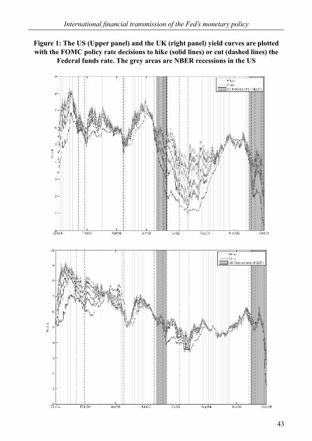
The dataset covers the period from January 1994 to the end of December 2008 and contains 3912 daily observations of the 6-month U.S. Dollar and G.B. Pound Libor rates, and plain vanilla fixed-for-floating interest rate swap rates from the two countries with maturities of 2, 3, 5, 7 and 10 years12. All the yields are converted to continuously compounded assuming semi-annual compounding13. The two curves are illustrated in Figure 1. On the short end, the 6-month Libor rates are corrected for the consequences of the credit disruption initiated in August 2007 and lasted until the end of the sample. For this time period, I simply use the 6-month Overnight Indexed Swap (OIS) rates in two currencies plus the average OIS - Libor spread for the entire sample14. In such a way, the short rate in the sample reflects the average credit conditions throughout the sample and excludes the spike in the Libor rates after the Lehman Brothers bankruptcy. During the considered time period, there were indeed several other episodes with particularly tight credit conditions in both the U.S. and the U.K., most notably the “Asian crisis” in July 1997, the “Russian crisis” in August 1998 and the “Dot-com bubble” burst in early 2000. Yet, on all these occasions there was no significant divergence of the Libor rates from the respective OIS rates in the two countries, nor from the respective Treasuries securities’ yields. Regarding the mid- and longer-term maturities, the swap rates are used mainly for two reasons. First, they are often regarded as “true” constant maturity yield data15 and thus not a subject to approximation error of bootstrapping and interpolation techniques. In addition, the swap rates imply a limited credit risk premium, as in most cases only the intermediate cash-flows are exchanged. The preliminary data inspection shows that the spread, as much

12 The Libor rates are obtained from daily fixings by the British Bankers Association while the swap rates are indicative mid-quotes averaged across many data providers. Both series are available on Bloomberg and the fixing time for the swap rates is set to 17:00 hours New York time.13 See (Hull, 2008).14 The OIS rates are also available on Bloomberg from beginning of 2001. The average OIS - Libor spread in the U.S. case was 11 basis points, and in the U.K. case 29 basis points.15 See (Dai and Singleton, 2000).


10

Nikola Mirkov

as the change in the spread, between the swap rates and off-the-run treasuries (in the U.S.) and the gilts (in the U.K.) of the corresponding maturity is minor, also around the Lehman Brothers bankruptcy and the subsequent credit disruption in October 2008.

2.2 Fed policy actions

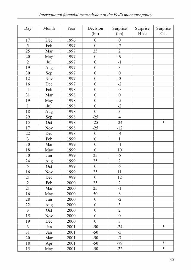
The dataset includes 125 policy meetings of the Federal Open Market Committee (FOMC) that resulted in an interest rate decision16. The starting policy action was an interest rate hike delivered on the 4th of February 1994. With this particular decision, the Fed started communicating the policy rate at the end of each meeting and the procedure has not been changed ever since17. The last decision in the sample was made on the 16th December 2008 in the midst of the recent financial crisis, when the Fed decided to cut the reference rate by 75 basis points to the target range 0 - 1/4 percent. Out of 125 FOMC meetings, 15 decisions are identified as “surprise changes” of the Federal Funds target rate. Following (Kuttner, 2001)18, I first construct a measure of the “surprise element” in Federal Funds target changes using the Federal Funds futures data from Chicago Mercantile Exchange. Secondly, different policy actions are characterised as expected or unexpected. In the construction of the policy surprise indicator, the change in the Fed target rate implied by the current-month futures contract on (monthly) average Federal Funds rate is considered. For a Fed decision that took place at day d of the month m, the unexpected change in the policy rate, scaled up by the factor that takes into account the number of days in the month affected by the change is calculated as:

(1)

where D is the number of days in the current month and Fm,d is the Fed Funds rate implied by the current-month futures contract value. If a policy decision was widely expected, the above change should be close to zero. In order to minimise the effect of month-end noise, I calculate an unscaled change for any decisions that came in place in the last 10 calendar days of any month19. Results are shown in Table 1 in the Appendix. Once constructed the surprise index, a “surprise change” is considered to be any

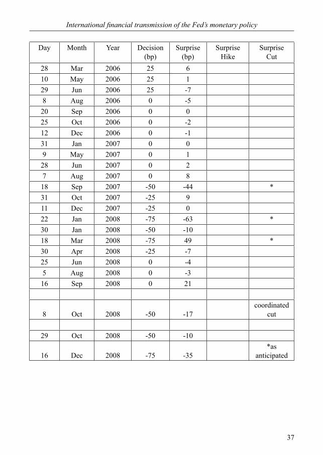
16 During the period, the FOMC delivered 126 policy rate decisions, out of which the interest rate cut delivered on the 8th of October 2008 was coordinated with, among others, the Bank of England (BoE). Consequently, this particular decision is excluded from the set.17 See (Piazzesi, 2005; Gurkaynak, Sack and Swanson, 2005). The starting date in the sample has been chosen accordingly.18 See also (Bernanke and Kuttner, 2005; Gurkaynak et al., 2005).19 Kuttner (2001) proposes 3 days for the same purpose. 10 days are chosen to bring the measure closer to what previous studies using the tick-by-tick data produced, most notably (Fleming and Piazzesi, 2005).


11


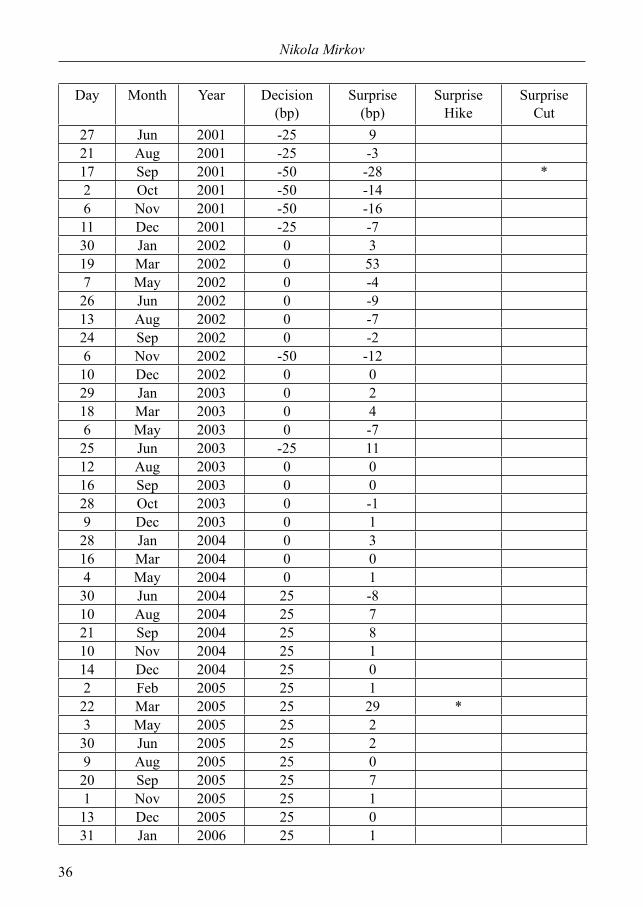
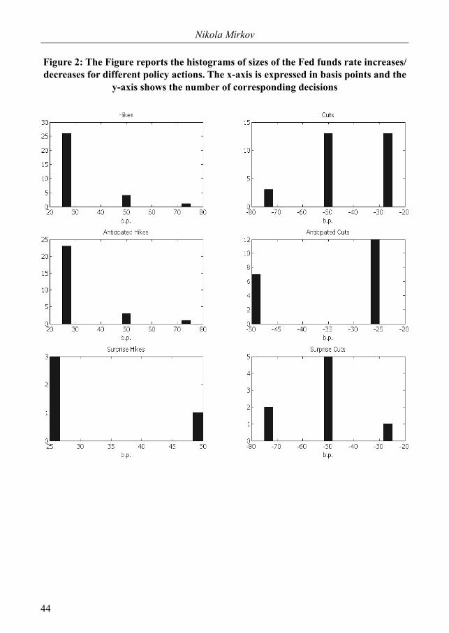
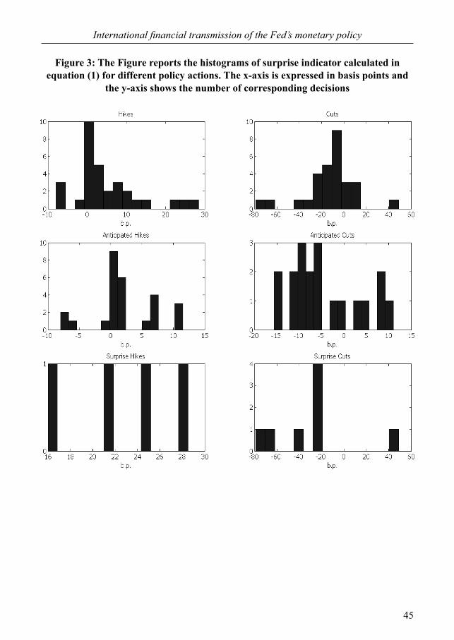
difference calculated in (1) that exceeds a two thirds of the usual 25 basis points move in any direction, namely under -16 and above +16 basis points. The two-thirds threshold was chosen as an arguably reasonable portion of the usual policy move, above which the move might be considered as a surprise one20. Out of 125 policy actions, 15 decisions are classified as “surprise moves” of the Fed. Specifically, out of 31 decisions opting for an interest rate hike, four seem to have surprised the markets. The three of them were brought in 1994 and one was delivered on 22nd of March 2005, in a series of rate hikes lasting from June 2004 to June 2006. Two decisions are considered as unexpected holds, namely the one delivered on the 19th of March 2002 and the one on the 18th of September 2008. The remaining 9 policy actions are considered as surprise target rate cuts and are equally spaced between the dot-com crisis at the beginning of 2000’s and the sub-prime crisis. Roughly half of these are delivered after an unscheduled meeting of the Fed21. There were overall 28 Fed decisions to cut the target rate. To illustrate the splits, Figure 2 reports the histograms of the size of policy rate changes for single “types” of policy decisions. It shows that the moves larger than 25 basis points tend to be classified as surprise moves, especially for the interest rate cuts. Also to notice is that expansionary policy decisions seem more likely to come at a surprise and that those decisions in the sample were on average higher in magnitude than the hiking decisions. Figure 3 illustrates the distributions of the surprise indicator, again conditional on different policy actions. The magnitude of the indicator seem to be again much higher around the policy rate cuts. This might not be surprising, as the decisions to cut the policy rate are usually delivered in times of elevated uncertainty and sometimes after an unscheduled meeting22. Finally, a brief comment regarding the FOMC decision on the 16th of December 2008, when the policy rate reached the target range 0 - 25 basis points, is warranted. It seems that the futures market was actually ”surprised” only by the magnitude of this final rate cut, where the scaled one day changed of the Fed futures was 35 basis points. Considering the size of the reserve balances of depository institutions at Federal Reserve banks at that time, the amount of monetary easing seem to have front-run the effective Federal funds rate23. For this reason, I do not consider this last Fed decision in the sample as a “surprise move” and re-classifying it to “anticipated” does not change the results.

20 Altering the threshold to 13 bp (assuming a “more-than-a-half” rule) makes the Fed funds cuts from 2nd October 2001 and 6th November 2001 become surprise cuts. Changing the cut-off around 16bp also does not alter the split significantly. The key results remain in both cases. Finally, increasing the cut-off to one entire move (25bp) would classify only few decisions as surprise.21 Namely, on the 15th of October 1998, 3rd of January 2001, the 18th of April 2001, the 17th of September 2001, and the 22nd of January 2008.22 The highest reading of the indicator of minus 68 basis points followed from the unscheduled meeting of the Federal Open Market Committee (FOMC) on the 22nd of January 2008, the details are reported in Table 1.23 See (Taylor, 2010).


12

Nikola Mirkov

3 Model

The following Section presents the two-country model where the home country (e.g. the United States) market prices of risk are priced into foreign bond markets (e.g. the United Kingdom). The key assumption is that the financial markets are perfectly integrated24 and complete25.

3.1 General Pricing Equation

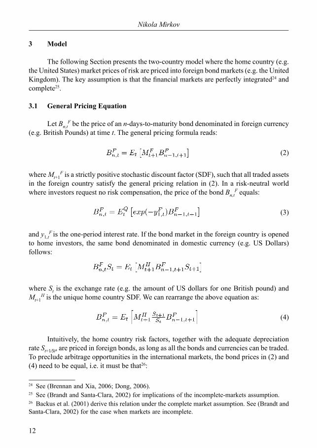
Let Bn,tF be the price of an n-days-to-maturity bond denominated in foreign currency

(e.g. British Pounds) at time t. The general pricing formula reads:

(2)

where Mt+1F is a strictly positive stochastic discount factor (SDF), such that all traded assets

in the foreign country satisfy the general pricing relation in (2). In a risk-neutral world where investors request no risk compensation, the price of the bond Bn,t

F equals:

(3)

and y1,tF is the one-period interest rate. If the bond market in the foreign country is opened

to home investors, the same bond denominated in domestic currency (e.g. US Dollars) follows:

where St is the exchange rate (e.g. the amount of US dollars for one British pound) and Mt+1

H is the unique home country SDF. We can rearrange the above equation as:

(4)

Intuitively, the home country risk factors, together with the adequate depreciation rate St+1⁄St, are priced in foreign bonds, as long as all the bonds and currencies can be traded. To preclude arbitrage opportunities in the international markets, the bond prices in (2) and (4) need to be equal, i.e. it must be that26:

24 See (Brennan and Xia, 2006; Dong, 2006).25 See (Brandt and Santa-Clara, 2002) for implications of the incomplete-markets assumption.26 Backus et al. (2001) derive this relation under the complete market assumption. See (Brandt and Santa-Clara, 2002) for the case when markets are incomplete.


13


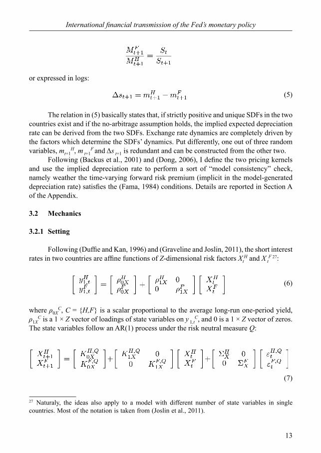
or expressed in logs:

(5)

The relation in (5) basically states that, if strictly positive and unique SDFs in the two countries exist and if the no-arbitrage assumption holds, the implied expected depreciation rate can be derived from the two SDFs. Exchange rate dynamics are completely driven by the factors which determine the SDFs’ dynamics. Put differently, one out of three random variables, mt+1

H, m t+1F and Δs t+1 is redundant and can be constructed from the other two.

Following (Backus et al., 2001) and (Dong, 2006), I define the two pricing kernels and use the implied depreciation rate to perform a sort of “model consistency” check, namely weather the time-varying forward risk premium (implicit in the model-generated depreciation rate) satisfies the (Fama, 1984) conditions. Details are reported in Section A of the Appendix.

3.2 Mechanics

3.2.1 Setting

Following (Duffie and Kan, 1996) and (Graveline and Joslin, 2011), the short interest rates in two countries are affine functions of Z-dimensional risk factors Xt

H and X tF 27:

(6)

where ρ0XC, C = {H,F} is a scalar proportional to the average long-run one-period yield,

ρ1XC is a 1 × Z vector of loadings of state variables on y 1,t

C, and 0 is a 1 × Z vector of zeros. The state variables follow an AR(1) process under the risk neutral measure Q:

(7)

27 Naturaly, the ideas also apply to a model with different number of state variables in single countries. Most of the notation is taken from (Joslin et al., 2011).


14

Nikola Mirkov

where K1XC,Q is the feedback matrix, Σ X

C is the variance-covariance matrix of the normally distributed error term εt

C,Q ~ N(0, 1). The zero restrictions in equations (6) and (7) have two important implications. First, the state variables in single countries under Q drive one-period yields in those countries only. As the short-rate is closely related to the monetary policy rate instrument, the zero restrictions on the one-period loadings intuitively imply, that the respective monetary policy makers mostly regard domestic variables of interest, when delivering a policy rate decision. Secondly, the co-movement between the risk factors in two countries is not allowed under the Q measure. Both implications result in single countries cross-sections of yields being driven by the domestic state-variables only. An obvious disadvantage of it is that the model cannot accommodate common risk factors for the two countries yield curves28. Yet the zero restrictions prove to be useful in the analysis presented here, as the model assigns a minor role of the US factors in explaining the UK yields and term premia. Since one would expect that the US yields (and not the UK yields) are particularly responsive to the Fed decisions, minimising their role in the model might offer more “conservative” results in assessing the reaction of the UK yield curve to policy rate decisions in the US. Combining the two equations and assuming joint log-normality of the stochastic discount factor and the bond prices in the general pricing equation (2), it can be shown that the n-days to maturity zero-coupon yields in the two countries are functions of the respective state variables:

(8)

where:

Differently from Q dynamics, the pricing factors’ under physical measure P are allowed to co-move. Once more, the state variables follow the AR(1) process:

(9)

where the upper-left and the lower-right blocks of the matrix ΣXP are equal to the matrices Σ

28 Diebold and Li (2006) for example find a strong empirical support of a common level factor in international bond markets. See also (Leippold and Wu, 2002; Dong, 2006).


15


XH and ΣX

F , respectively. Yet the off-diagonal blocks of K 1XP and Σ X

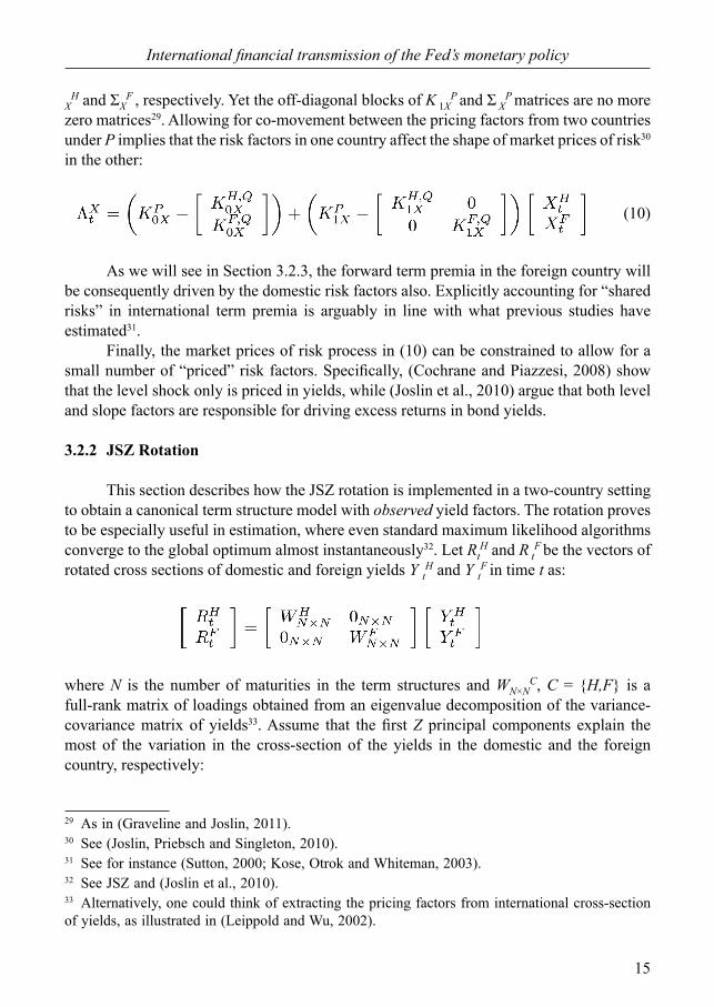
P matrices are no more zero matrices29. Allowing for co-movement between the pricing factors from two countries under P implies that the risk factors in one country affect the shape of market prices of risk30 in the other:

(10)

As we will see in Section 3.2.3, the forward term premia in the foreign country will be consequently driven by the domestic risk factors also. Explicitly accounting for “shared risks” in international term premia is arguably in line with what previous studies have estimated31. Finally, the market prices of risk process in (10) can be constrained to allow for a small number of “priced” risk factors. Specifically, (Cochrane and Piazzesi, 2008) show that the level shock only is priced in yields, while (Joslin et al., 2010) argue that both level and slope factors are responsible for driving excess returns in bond yields.

3.2.2 JSZ Rotation

This section describes how the JSZ rotation is implemented in a two-country setting to obtain a canonical term structure model with observed yield factors. The rotation proves to be especially useful in estimation, where even standard maximum likelihood algorithms converge to the global optimum almost instantaneously32. Let Rt

H and R tF be the vectors of

rotated cross sections of domestic and foreign yields Y tH and Y tF in time t as:

where N is the number of maturities in the term structures and WN×NC, C = {H,F} is a

full-rank matrix of loadings obtained from an eigenvalue decomposition of the variance-covariance matrix of yields33. Assume that the first Z principal components explain the most of the variation in the cross-section of the yields in the domestic and the foreign country, respectively:

29 As in (Graveline and Joslin, 2011).30 See (Joslin, Priebsch and Singleton, 2010).31 See for instance (Sutton, 2000; Kose, Otrok and Whiteman, 2003).32 See JSZ and (Joslin et al., 2010).33 Alternatively, one could think of extracting the pricing factors from international cross-section of yields, as illustrated in (Leippold and Wu, 2002).


16

Nikola Mirkov

with:

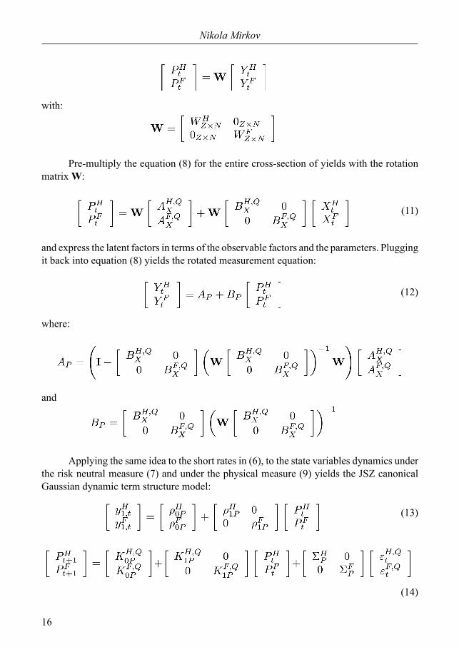
Pre-multiply the equation (8) for the entire cross-section of yields with the rotation matrix W:

(11)

and express the latent factors in terms of the observable factors and the parameters. Plugging it back into equation (8) yields the rotated measurement equation:

(12)

where:

and

Applying the same idea to the short rates in (6), to the state variables dynamics under the risk neutral measure (7) and under the physical measure (9) yields the JSZ canonical Gaussian dynamic term structure model:

(13)

(14)


17


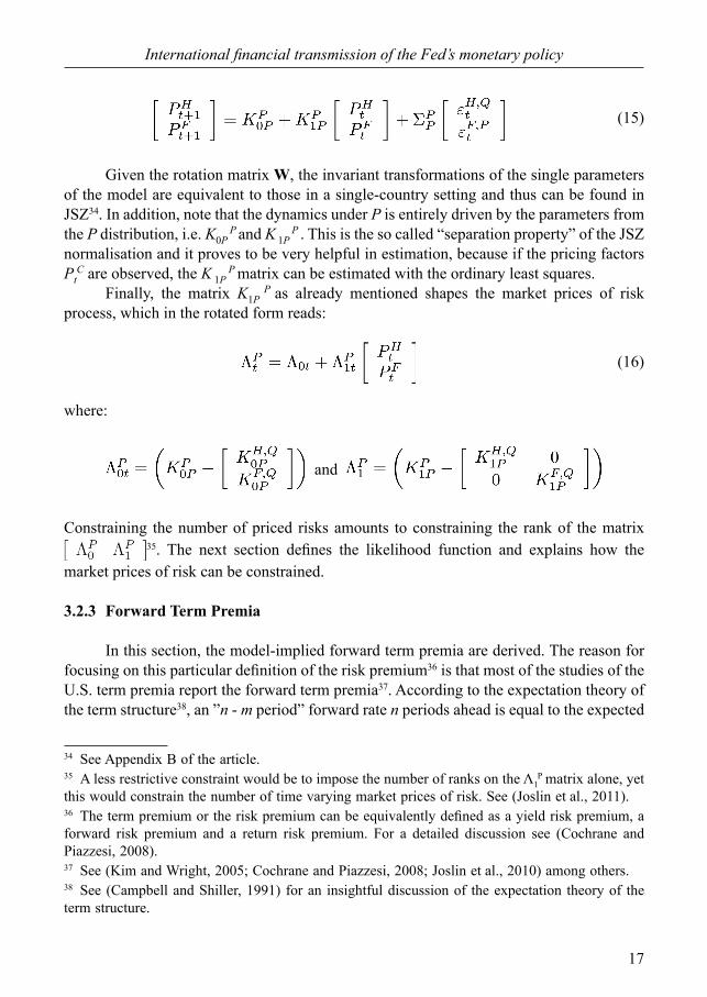
(15)

Given the rotation matrix W, the invariant transformations of the single parameters of the model are equivalent to those in a single-country setting and thus can be found in JSZ34. In addition, note that the dynamics under P is entirely driven by the parameters from the P distribution, i.e. K0P

P and K 1P P . This is the so called “separation property” of the JSZ

normalisation and it proves to be very helpful in estimation, because if the pricing factors Pt

C are observed, the K 1P P matrix can be estimated with the ordinary least squares.

Finally, the matrix K1P P as already mentioned shapes the market prices of risk

process, which in the rotated form reads:

(16)

where:

and

Constraining the number of priced risks amounts to constraining the rank of the matrix 35. The next section defines the likelihood function and explains how the

market prices of risk can be constrained.

3.2.3 Forward Term Premia

In this section, the model-implied forward term premia are derived. The reason for focusing on this particular definition of the risk premium36 is that most of the studies of the U.S. term premia report the forward term premia37. According to the expectation theory of the term structure38, an ”n - m period” forward rate n periods ahead is equal to the expected

34 See Appendix B of the article.35 A less restrictive constraint would be to impose the number of ranks on the Λ1

P matrix alone, yet this would constrain the number of time varying market prices of risk. See (Joslin et al., 2011).36 The term premium or the risk premium can be equivalently defined as a yield risk premium, a forward risk premium and a return risk premium. For a detailed discussion see (Cochrane and Piazzesi, 2008).37 See (Kim and Wright, 2005; Cochrane and Piazzesi, 2008; Joslin et al., 2010) among others.38 See (Campbell and Shiller, 1991) for an insightful discussion of the expectation theory of the term structure.


18

Nikola Mirkov

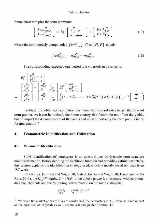
future short rate plus the term premium:

(17)

where the continuously compounded equals:

(18)

The corresponding expected one-period rate n periods in advance is:

I subtract the obtained expectation part from the forward rates to get the forward term premia. As it can be noticed, the home country risk factors do not affect the yields, but do impact the decomposition of the yields and most importantly the term premia in the foreign country39.

4. Econometric Identification and Estimation

4.1 Parameter Identification

Solid identification of parameters is an essential part of dynamic term structure models estimation. Before defining the likelihood function and providing estimation details, this section explains the identification strategy used, which is mostly based on ideas from JSZ work. Following (Hamilton and Wu, 2010; Calvet, Fisher and Wu, 2010; Bauer and de los Rios, 2011), the K1X

C,Q matrix, C = {H,F} is set to be a power law structure, with zero non-diagonal elements and the following power relation on the matrix’ diagonal:

39 Yet when the market prices of risk are constrained, the parameters in K1PP exercise some impact

on the cross-section of yields as well, see the last paragraph of Section 4.2.


19


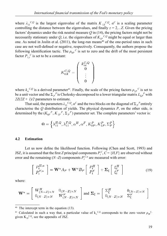
where λ11C,Q is the largest eigenvalue of the matrix K 1X

C,Q, αC is a scaling parameter controlling the distance between the eigenvalues, and finally z = 2,...Z. Given the pricing factors’ dynamics under the risk neutral measure Q in (14), the pricing factors might not be necessarily stationary under Q, i.e. the eigenvalues of K1P

C,Q might be equal or larger than one. As noted in Joslin et al. (2011), the long-run means40 of the one-period rates in such case are not well-defined or negative, respectively. Consequently, the authors propose the following identification tactic. The ρ0P

C is set to zero and the drift of the most persistent factor P1,t

C is set to be a constant:

where k∞C,Q is a derived parameter41. Finally, the scale of the pricing factors ρ1P C is set to

be a unit vector and the Σ P P is Cholesky-decomposed to a lower triangular matrix LΣP

P with 2Z(2Z + 1)⁄2 parameters to estimate. That said, the parameters λ11

C,Q, αC and the two blocks on the diagonal of Σ P P entirely

characterise the Q distribution of yields. The physical dynamics P, on the other side, is determined by the (K0P

P , K 1P P , Σ P

P ) parameter set. The complete parameters’ vector is:

4.2 Estimation

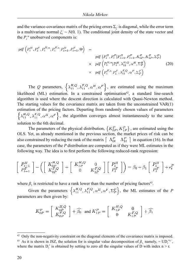
Let us now define the likelihood function. Following (Chen and Scott, 1993) and JSZ, it is assumed that the first Z principal components Pt

C, C = {H,F} are observed without error and the remaining (N -Z) components Pt

C,u are measured with error:

(19)

where:

and

40 The intercept term in the equation (13).41 Calculated in such a way that, a particular value of k∞

C,Q corresponds to the zero vector ρ0PC,

given K1PC,Q, see the appendix of JSZ.


20

Nikola Mirkov

and the variance-covariance matrix of the pricing errors Σξ· is diagonal, while the error term is a multivariate normal ξt

· ~ N(0, 1). The conditional joint density of the state vector and the Pt

·u unobserved components is:

(20)

The Q parameters, , are estimated using the maximum likelihood (ML) estimation. In a constrained optimisation42, a standard line-search algorithm is used where the descent direction is calculated with Quasi-Newton method. The starting values for the covariance matrix are taken from the unconstrained VAR(1) estimation of the pricing factors. Departing from randomly chosen values of parameters

, the algorithm converges almost instantaneously to the same

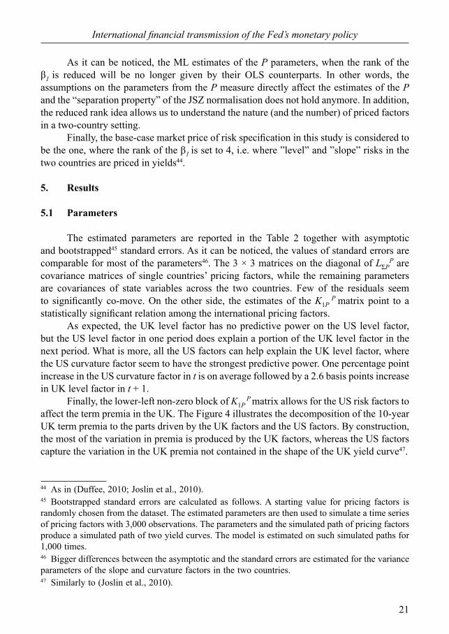
solution to the 6th decimal. The parameters of the physical distribution, , are estimated using the OLS. Yet, as already mentioned in the previous section, the market prices of risk can be also constrained by reducing the rank of the matrix in equation (16). In that case, the parameters of the P distribution are computed as if they were ML estimates in the following way. The idea is to first perform the following reduced-rank regression:

where β1 is restricted to have a rank lower than the number of pricing factors43. Given the parameters , the ML estimates of the P parameters are then given by:

and

42 Only the non-negativity constraint on the diagonal elements of the covariance matrix is imposed.43 As it is shown in JSZ, the solution for is singular value decomposition of β1, namely, = UDr

*V ′, where the matrix Dr

* is obtained by setting to zero all the singular values of D with index n > r.


21


As it can be noticed, the ML estimates of the P parameters, when the rank of the β1 is reduced will be no longer given by their OLS counterparts. In other words, the assumptions on the parameters from the P measure directly affect the estimates of the P and the “separation property” of the JSZ normalisation does not hold anymore. In addition, the reduced rank idea allows us to understand the nature (and the number) of priced factors in a two-country setting. Finally, the base-case market price of risk specification in this study is considered to be the one, where the rank of the β1 is set to 4, i.e. where ”level” and ”slope” risks in the two countries are priced in yields44.

5. Results

5.1 Parameters

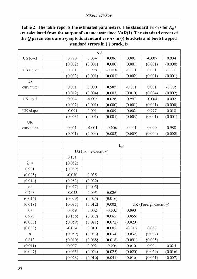
The estimated parameters are reported in the Table 2 together with asymptotic and bootstrapped45 standard errors. As it can be noticed, the values of standard errors are comparable for most of the parameters46. The 3 × 3 matrices on the diagonal of LΣP

P are covariance matrices of single countries’ pricing factors, while the remaining parameters are covariances of state variables across the two countries. Few of the residuals seem to significantly co-move. On the other side, the estimates of the K1P

P matrix point to a statistically significant relation among the international pricing factors. As expected, the UK level factor has no predictive power on the US level factor, but the US level factor in one period does explain a portion of the UK level factor in the next period. What is more, all the US factors can help explain the UK level factor, where the US curvature factor seem to have the strongest predictive power. One percentage point increase in the US curvature factor in t is on average followed by a 2.6 basis points increase in UK level factor in t + 1. Finally, the lower-left non-zero block of K1P

P matrix allows for the US risk factors to affect the term premia in the UK. The Figure 4 illustrates the decomposition of the 10-year UK term premia to the parts driven by the UK factors and the US factors. By construction, the most of the variation in premia is produced by the UK factors, whereas the US factors capture the variation in the UK premia not contained in the shape of the UK yield curve47.

44 As in (Duffee, 2010; Joslin et al., 2010).45 Bootstrapped standard errors are calculated as follows. A starting value for pricing factors is randomly chosen from the dataset. The estimated parameters are then used to simulate a time series of pricing factors with 3,000 observations. The parameters and the simulated path of pricing factors produce a simulated path of two yield curves. The model is estimated on such simulated paths for 1,000 times.46 Bigger differences between the asymptotic and the standard errors are estimated for the variance parameters of the slope and curvature factors in the two countries.47 Similarly to (Joslin et al., 2010).


22

Nikola Mirkov

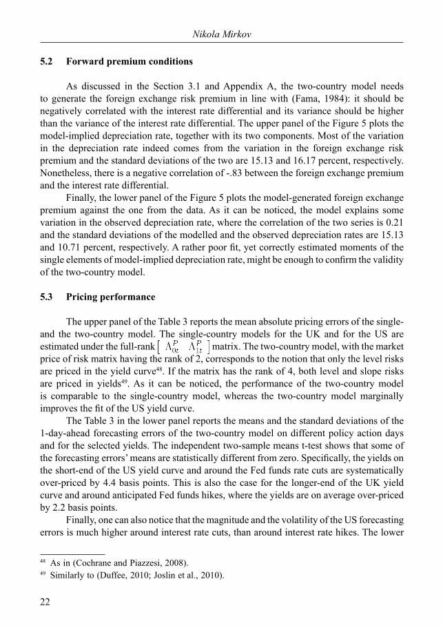
5.2 Forward premium conditions

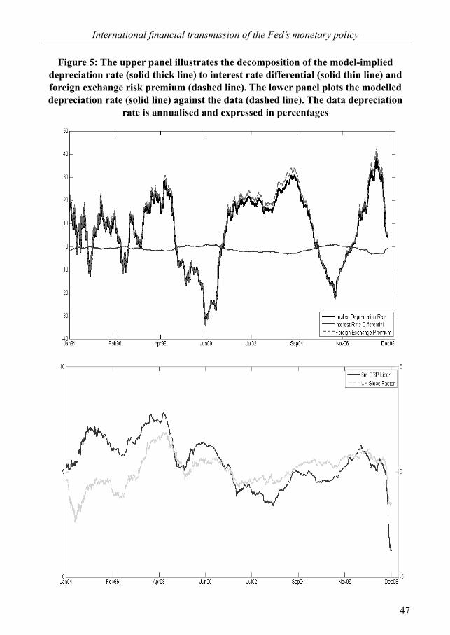
As discussed in the Section 3.1 and Appendix A, the two-country model needs to generate the foreign exchange risk premium in line with (Fama, 1984): it should be negatively correlated with the interest rate differential and its variance should be higher than the variance of the interest rate differential. The upper panel of the Figure 5 plots the model-implied depreciation rate, together with its two components. Most of the variation in the depreciation rate indeed comes from the variation in the foreign exchange risk premium and the standard deviations of the two are 15.13 and 16.17 percent, respectively. Nonetheless, there is a negative correlation of -.83 between the foreign exchange premium and the interest rate differential. Finally, the lower panel of the Figure 5 plots the model-generated foreign exchange premium against the one from the data. As it can be noticed, the model explains some variation in the observed depreciation rate, where the correlation of the two series is 0.21 and the standard deviations of the modelled and the observed depreciation rates are 15.13 and 10.71 percent, respectively. A rather poor fit, yet correctly estimated moments of the single elements of model-implied depreciation rate, might be enough to confirm the validity of the two-country model.

5.3 Pricing performance

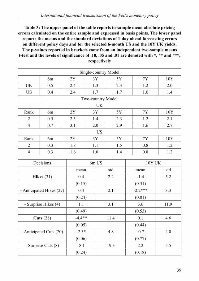
The upper panel of the Table 3 reports the mean absolute pricing errors of the single- and the two-country model. The single-country models for the UK and for the US are estimated under the full-rank matrix. The two-country model, with the market price of risk matrix having the rank of 2, corresponds to the notion that only the level risks are priced in the yield curve48. If the matrix has the rank of 4, both level and slope risks are priced in yields49. As it can be noticed, the performance of the two-country model is comparable to the single-country model, whereas the two-country model marginally improves the fit of the US yield curve. The Table 3 in the lower panel reports the means and the standard deviations of the 1-day-ahead forecasting errors of the two-country model on different policy action days and for the selected yields. The independent two-sample means t-test shows that some of the forecasting errors’ means are statistically different from zero. Specifically, the yields on the short-end of the US yield curve and around the Fed funds rate cuts are systematically over-priced by 4.4 basis points. This is also the case for the longer-end of the UK yield curve and around anticipated Fed funds hikes, where the yields are on average over-priced by 2.2 basis points. Finally, one can also notice that the magnitude and the volatility of the US forecasting errors is much higher around interest rate cuts, than around interest rate hikes. The lower

48 As in (Cochrane and Piazzesi, 2008).49 Similarly to (Duffee, 2010; Joslin et al., 2010).


23


forecasting performance might be due to elevated macroeconomic uncertainty during the circumstances in which the decisions to cut the Fed funds rate are usually delivered. The model is thus more likely to be “wrong” around those decisions. The same pattern does not seem to hold for the UK yields.

5.4 Reactions to the Fed decisions

As already mentioned, different policy rate decisions of the Fed are classified across two dimensions and used to analyse the reaction of yields to those decisions. As there might be no particular reason to assume that yields respond symmetrically to contractionary and expansionary monetary policy shocks, the splitting should provide a sort of generalisation of policy shock notion and flexibility in estimating the response. This section reports both dynamic and instantaneous reaction of the UK yield curve to the Fed policy actions.

5.4.1 Impulse response functions

In a VAR- or term structure model analysis, general impulse response function of (Pesaran and Shin, 1998) is usually used to describe the reaction of state variables or yields to one standard deviation shock in another state variable50. In such a case, the dynamic reaction of yields to a monetary policy shock could be analysed by considering the one-period interest rate in the sample as the monetary policy instrument and then using it as one of the state variables51. In this study, the one-period US interest rate is the 6-month USD Libor. Even though the short-term Libor rates closely co-move with the Fed funds rate, the spread between the funds rate and the Libor rates might not be necessarily constant, because the latter include credit risk premium52. Alternatively, the idea here would be to extract the shocks from the models’ residuals around policy action days. From every realisation of the state variable vector Pd on a policy action day d, its ex-ante expectation E[Pd | Id-1 ] is subtracted. The residuals obtained in this way are then grouped to classes (e.g. hikes) and used to calculate impulse response functions. The Appendix B illustrates the idea and the Figure 6 reports the average response functions of the 6-month and the 10-year yields in the two countries together with 90 percent confidence intervals. To begin with, the UK short rate reacts negatively to both hikes and cuts of the Federal funds rate. On the other side, the sign of the US short rate response is analogous to direction of the policy rate move and both UK and US short rates react more strongly to interest rate cuts. Section 5.4.2 shows that the negative reaction of the UK short rate

50 See for instance (Evans and Marshall, 1998; Söderlind, 2010) or (Kaminska, 2008).51 In the JSZ framework, this can be done by setting the element (1,1) of the rotation matrix WZ×N in (11) to 1 and other elements of the first row of the matrix to 0.52 An insightful way of including the Fed policy rate to the model estimation is proposed in (Piazzesi, 2005), who uses the effective Fed funds rate as the state variable.


24

Nikola Mirkov

to contractionary policy shocks in the US might be explained by a fall in estimated term premia. Moving to the longer-end of the curve, the yields reaction seem to be much lower, which is in line with (Evans and Marshall, 1998). Interestingly, the yield curves in both countries seem to shift in a parallel fashion around Fed funds rate hikes and steepen around rate cuts. The letter result is also in line with (Evans and Marshall, 1998), whereas the magnitude of the short rate reaction is estimated to be lower. Specifically, the authors estimate that a one-standard deviation monetary policy shock, corresponding to circa 50bp increase/decrease in the Federal funds rate, produces a 20 basis points rise/fall in a 1-month interest rate. The analogous estimate in this paper is approximately 7 basis points fall in the 6-month USD Libor. Finally, it might be important to notice that the estimated state variables are substantially persistent, given that the data frequency is daily. Consequently, the reported lengths of shocks’ persistence should be considered as indicative and one possible remedy would be to estimate the state variable process on monthly data and then use the extracted residuals to ”shock” the system, as previously explained53.

5.4.2 Instantaneous reactions

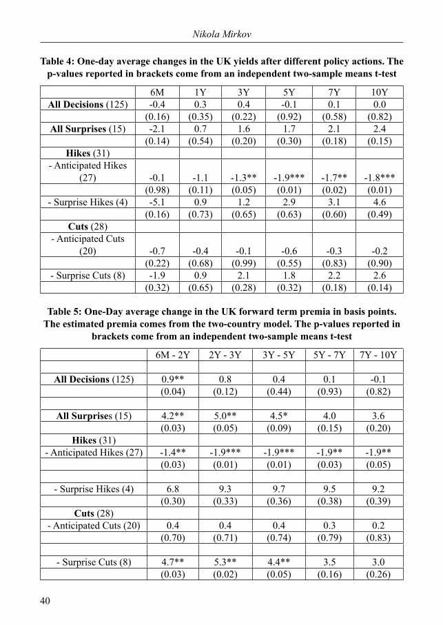
Table 4 reports one-day average change in the UK yields followed by different policy rate decisions of the Fed. The changes are expressed in basis points and compared with the average one-day changes on non-policy days in an independent two-sample t-test of means54. The values in brackets are corresponding p-values of the test statistic. As it can be noticed, there is a statistically significant decrease in the UK yields on the long-end of the curve, as an average change after anticipated decisions to hike the Fed funds rate. This might not sound intuitive, because the “anticipated” decisions should be priced in yields. Yet, if the Fed funds futures market correctly anticipated a policy decision, it does not necessarily mean that the rates market followed suit. The decisions are classified into expected or surprise policy actions by only looking at the Fed funds futures quotes and the corresponding implicit Fed funds rate “expectation”. In addition to this, (Bernanke and Kuttner, 2005) notice that asset prices need not to respond only to surprise moves of the Fed, but also to revisions in expectation about future policy, which may also result from a policy decision55. Why do the long-term UK yields fall after an anticipated hike of the Federal funds rate? As the Table 5 reports, the fall in yields seem to be given mostly by the decrease in the

53 A similar idea was used in (Bauer and Rudebusch, 2011) to estimate future short-rate expectations when decomposing the US yield curve.54 As the fixings for the Libor rates take place around 13:00 hours London time, so before the FOMC statement is released on a given day d, the one-day changes of Libor rates are calculated by using d + 1 and d observations.55 Every policy rate decision is announced together with a brief communiqué on the general economic assessment, in the form of so called Federal Open Market Committee (FOMC) Statement.


25


term premia. If the estimated time-varying premia can be regarded as uncertainty around future short-rate expectation i.e. a “deviation” from expectation hypothesis56, then the anticipated hike decision of the Fed seem to reduce that uncertainty. The negative reaction of the premia is almost equal in magnitude across the maturity spectrum. Since the future short-rate expectations for maturities under 5Y slightly rise57, only the yields on the longer-end seem to be affected by the shift. The average increase of the Fed funds rate by 29bp (on 27 anticipated hike decisions) is estimated to cause on average a 2bp fall in 5 to 10Y maturities yields. Almost entire reaction is estimated to be driven by the fall in longer term premia by approximately the same amount. If anticipated rate decisions provoke a decrease in the premia, a surprise policy actions should have an opposite effect. Indeed, the Table 5 reports statistically significant and positive 1-day change of the premia after both unexpected policy rate hikes and cuts of the Fed funds rate. There is on average a 4.5 bp increase in the premia around short- and medium term maturities after an unexpected interest rate cut. As only 4 decisions to increase the Fed funds rate are labelled as unexpected, the reaction of the premia around those days is not statistically significant. Still, the average change of the premia after all surprises are statistically different from the average change on a non-policy day. The Table 6 confirms these conclusions for the single-country model for the UK yield curve and the results do not change when the market prices of risk are constrained.

5.4.3 Robustness check: Post-2007 period

On the 9th of August 2007, the interbank markets of the United States and the euro area came under unexpected and severe strains58, after months of falling house prices and adverse events in the US sub-prime mortgage market. The US policy-maker, concerned about the tightening of credit conditions, lowered the Federal funds rate by 50 basis points on the 18th of September 2007 and embarked on a stream of interest rate cuts. In the UK, the Bank of England started to decrease the reference rate in December 2007 and continued to do so on several occasions until the end of the sample59. Highly correlated policy paths during this period, together with globally deteriorating growth prospects and dire credit conditions, might be excessively driving the results presented above. For this reason, I re-estimate the two-country model on the sub-sample excluding the period from the beginning of August 2007 until the end of the sample. The estimated term-premia average changes are reported in the Table 7. As it can be noticed, the main result remains. The one-day average change in the term premia, after an anticipated

56 See (Kim and Orphanides, 2007).57 Unfortunately, the changes in future short-rate expectations are not statistically significant and thus not reported.58 See (Borio, 2008).59 The bank rate was reduced on 7th of February, 10th of April, 8th of October, 6th of November and 4th of December 2008. The details about the decisions can be found here.


26

Nikola Mirkov

hike of the Federal funds rate, is statistically different from zero. Nonetheless, there seem to be an increase in premia on short- and medium-term maturities, after the surprise policy actions of the Fed.

5.4.4 Robustness check: Weighted average response

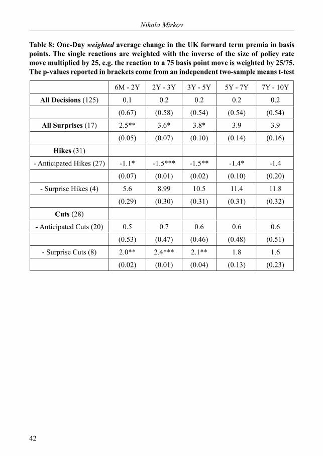
Another important check would be to control for the size heterogeneity of policy moves across and within different groups of policy actions. As we have seen in the Section 2.2, larger changes of the Fed funds rate are usually communicated after expansionary decisions. In addition, most of the surprise decisions are changes in the policy rate of more than 25 basis points, see Figure 3. Accordingly, the results might be driven by several extreme cases of substantial change in the policy rate and the subsequent reaction in the yields. To control for such effects, I calculate a weighted average reaction of the UK premia to different policy actions in the following way. All the one-day changes are multiplied by the inverse of the corresponding policy rate move times 25 (e.g. for a 50 basis points hike, the “weight” would be 25/50). The re-scaled changes are then summed up within a group of policy actions and divided by the number of decisions in the group. The outcome is an estimated one-day average change of the term premia, as a result of 25 basis points change in the policy rate and it is reported in Table 8. As expected, the magnitude of changes is somewhat lower, especially after the interest rate cuts. Still, the reaction of the premia to surprise policy moves is still statistically different from zero and independent of the direction of the policy move and there is a decrease in the premia at the medium and long-end of the curve as a result of anticipated hikes of the Fed funds rate.

6. Conclusion

International financial transmission of the US Federal Reserve can be studied by extracting monetary policy shocks from daily interest rate movements around the FOMC decisions. This study illustrates it by estimating a two-country term structure model on the US-UK data. There are several ways to go from here. One could use a latent-factor framework to allow the home country risk factors to explain movements in foreign term premia. The estimated factor loadings on one-period rates could provide insight into the nature of information used by the central banks in respective countries. Furthermore, it might be interesting to explore the extent to which a highly correlated or even common level and slope factors can be connected to the convergence in medium-term inflation expectations in the two countries, or to similar business cycles or policy instruments paths.

Acknowledgment

I gratefully acknowledge an invaluable and constant support of my doctoral advisor


27


Paul Söderlind. A great thanks to Francis Diebold, Lars Svensson, Hans Dewachter, Martin Brown, Herman K. van Dijk, Lukas Wager, Andreas Steinmayr, Norman Seeger, Kevin Lansing, Dagfinn Rime, seminar and conference participants at the University of St.Gallen, National Bank of Serbia, Norges Bank, the 5th CSDA International Conference and the 5th RGS Doctoral Conference in Economics. All remaining errors are my own. The views expressed in the paper are those of the author and do not necessarily represent those of the Swiss National Bank.

References

Backus, D., Foresi, S. and Telmer, C., 2001, ‘Affine Term Structure Models and the Forward Premium Anomaly’, Journal of Finance, 56, 1, pp. 279-304.

Bansal, R., 1997, ‘An Exploration of the Forward Premium Puzzle in Currency Markets’, Review of Financial Studies, 10, 2.

Bauer, G.H. and Antonio Diez de los Rios, 2011, ‘An International Dynamic Term Structure Model with Economic Restrictions and Unspanned Risks’, Working Paper.

Bauer, M.D. and Glenn D. Rudebusch, 2011, ‘The signaling channel for Federal Reserve bond purchases’, Technical report.

Bernanke, Ben S. and Kuttner, K.N., 2005, ‘What Explains the Stock Market’s Reaction to Federal Reserve Policy?” Journal of Finance, 60, 3, pp. 1221-1257, 06.

Borio, C., 2008, ‘The financial turmoil of 2007?: a preliminary assessment and some policy consideration’, BIS Working Papers No 251.

Brandt, M.W. and Santa-Clara, P, 2002, ‘Simulated likelihood estimation of diffusions with an application to exchange rate dynamics in incomplete markets’, Journal of Financial Economics, 63, 2, pp. 161-210.

Brennan, M.J. and Yihong Xia, 2006, ‘International Capital Markets and Foreign Exchange Risk’, Review of Financial Studies, 19, 3, pp. 753-795.

Calvet, L.E., Aldai Fisher and Liuren Wu, 2010, ‘Dimension-Invariant Dynamic Term Structures’, Working Paper.

Campbell, J.Y and Shiller, R.J., 1991, ‘Yield Spreads and Interest Rate Movements: A Bird’s Eye View’, Review of Economic Studies, 58, 3, pp. 495-514, May.

Canova, F., 2005, ‘The transmission of US shocks to Latin America’, Journal of Applied Econometrics, 20, 2, pp. 229-251.

Chen, Ren-Raw and Louis Scott, 1993, ‘Multi-Factor Cox-Ingersoll-Ross Models of the Term Structure: Estimates and Tests from a Kalman Filter Model’, Journal of Real Estate Finance and Economics, 27, 2.

Cochrane, J.H., 2006, ‘Comments on ‘Macroeconomic Implications of Changes in the Term Premium’ by Glenn Rudebusch, Brian Sack and Eric Swanson’, Working Paper.

Cochrane, J.H. and Piazzesi, M., 2002, ‘The Fed and Interest Rates - A High-Frequency Identification’, American Economic Review, 92, 2, pp. 90-95, May.


28

Nikola Mirkov

Cochrane, J.H. and Piazzesi, M., 2005, ‘Bond Risk Premia’, American Economic Review, 95, 1, pp. 138-160, March.

Cochrane, J.H. and Piazzesi, M., 2008, ‘Decomposing the Yield Curve’, Working Paper. Cooley, Th.F and Vincenzo Quadrini, 2001, ‘The Cost of Losing Monetary Independence:

The Case of Mexico’, Journal of Money, Credit and Banking, 33, 2, pp. 370-97, May. Cumby, R.E. and Obstfeld, M., 1985, ‘International Interest-Rate and Price-Level Linkages

Under Flexible Exchange Rates: A Review of Recent Evidence’, NBER Working Papers 0921, National Bureau of Economic Research, Inc.

Dai, Qiang and Singleton, K.J., 2000, ‘Specification Analysis of Affine Term Structure Models’, Journal of Finance, 55, 5, pp. 1943-1978, October.

Diebold, F.X. and Canlin Li, 2006, ‘Forecasting the term structure of government bond yields’, Journal of Econometrics, 130, 2, pp. 337-364, February.

Dong, S., 2006, ‘Monetary Policy Rules and Exchange Rates:A Structural VAR Identified by No Arbitrage’, No. 875, December.

Duffee, G., 2010, ‘Sharpe ratios in term structure models’, Economics Working Paper Archive 575, The Johns Hopkins University, Department of Economics.

Duffie, D. and Rui Kan, 1996, ‘A Yield-Factor Model Of Interest Rates’, Mathematical Finance, 6, 4, pp. 379-406.

Ehrmann, M. and Fratzscher, M., 2004, ‘Taking stock: monetary policy transmission to equity markets’, Working Paper Series 354, European Central Bank.

Ehrmann, M. and Fratzscher, M., 2006, ‘Global financial transmission of monetary policy shocks’, Working Paper Series 616, European Central Bank.

Engel, C., 1996, ‘The forward discount anomaly and the risk premium: A survey of recent evidence’, Journal of Empirical Finance, 3, 2, pp. 123-192, June.

Evans, C.L. and Marshall, D.A., 1998, ‘Monetary policy and the term structure of nominal interest rates: Evidence and theory’, Carnegie-Rochester Conference Series on Public Policy, 49, 0, pp. 53-111.

Fama, E.F., 1984, ‘Forward and spot exchange rates’, Journal of Monetary Economics, 14, 3, pp. 319-338, November.

Favero, C. and Giavazzi, F., 2008, ‘The ECB and the bond market’, European Economy - Economic Papers 314, Directorate General Economic and Monetary Affairs, European Commission.

Fleming, M.J. and Piazzesi, M., 2005, ‘Monetary Policy Tick-by-Tick’, Working Paper. Fraser, P. and Oluwatobi Oyefeso, 2005, ‘US, UK and European Stock Market Integration’,

Journal of Business Finance & Accounting, 32, 1-2, pp. 161-181. Graveline, J.J., 2006, ‘Exchange Rate Volatility and the Forward Premium Anomaly’,

Working Paper. Graveline, J.J. and Scott Joslin, 2011, ‘G10 Swap and Exchange Rates’, Working Paper. Gurkaynak, R.S, Brian Sack and Swanson, E., 2005, ‘Do Actions Speak Louder Than

Words? The Response of Asset Prices to Monetary Policy Actions and Statements’, International Journal of Central Banking, 1, 1, May.


29


Hamilton, J.D. and Jing, C. Wu, 2010, ‘Identification and Estimation of Affine-Term-Structure Models.”

Hansen, L.P. and Hodrick, R.J., 1983, ‘Risk Averse Speculation in the Forward Foreign Exchange Market: An Econometric Analysis of Linear Models’, in Exchange Rates and International Macroeconomics: National Bureau of Economic Research, Inc, pp. 113-152.

Hodrick, R.J., 1987, ‘The empirical evidence on the efficiency of forward and futures foreign exchange markets’, Harwood Academic Publishers, Chur, Switzerland, p. 174.

Hull, J.C., 2008, Options, Futures, and Other Derivatives with Derivagem CD (7th Edition): Prentice Hall, 7th edition.

Joslin, Scott, Priebsch, M., and Singleton, K.J., 2010, ‘Risk Premiums in Dynamic Term Structure Models with Unspanned Macro Risks”, The Journal of Finance, 69, 3, pp. 1197-1233, June 2014

Joslin, Scott, Singleton, K.J. and Haoxiang Zhu, 2011, ‘A New Perspective on Gaussian Dynamic Term Structure Models’, Review of Financial Studies.

Jotikasthira, Chotibhak, Anh Le, and Christian Lundblad, 2010, ‘Why Do Term Structures in Different Currencies Co-move?” Working Paper.

Kaminska, I., 2008, ‘A no-arbitrage structural vector autoregressive model of the UK yield curve’, Bank of England working papers 357, Bank of England.

Kim, D.H. and Orphanides, A., 2007, ‘The bond market term premium: what is it, and how can we measure it?” BIS Quarterly Review, June.

Kim, D.H. and Wright, J.H., 2005, ‘An arbitrage-free three-factor term structure model and the recent behavior of long-term yields and distant-horizon forward rates’, Technical report.

Kim, S., 2001, ‘International transmission of U.S. monetary policy shocks: Evidence from VAR’s’, Journal of Monetary Economics, 48, 2, pp. 339-372, October.

Kose, M. Ayhan, Christopher Otrok, and Whiteman, C.H., 2003, ‘International Business Cycles: World, Region, and Country-Specific Factors’, American Economic Review, 93, 4, pp. 1216-1239.

Kozicki, S. and Tinsley P.A., 2005, ‘What do you expect? Imperfect policy credibility and tests of the expectations hypothesis’, Journal of Monetary Economics, 52, 2, pp. 421-447, March.

Kuttner, K.N., 2001, ‘Monetary policy surprises and interest rates: Evidence from the Fed funds futures market’, Journal of Monetary Economics, 47, 3, pp. 523-544, June.

Leippold, M. and Liuren Wu, 2002, ‘Asset Pricing under the Quadratic Class’, Journal of Financial and Quantitative Analysis, 37, 02, pp. 271-295, June.

Mumtaz, H. and Surico, P., 2008, ‘Time-Varying Yield Curve Dynamics and Monetary Policy’, Bank of England Discussion Papers, No. 23, March.

Pesaran, H.H. and Yongcheol Shin, 1998, ‘Generalized impulse response analysis in linear multivariate models’, Economics Letters, 58, 1, pp. 17-29.

Piazzesi, M., 2005, ‘Bond Yields and the Federal Reserve’, Journal of Political Economy, 113, 2, pp. 311-344, April.


30

Nikola Mirkov

Rigobon, R. and Brian Sack, 2004, ‘The impact of monetary policy on asset prices’, Journal of Monetary Economics, 51, 8, pp. 1553-1575, November.

Rudebusch, G.D. and Tao Wu, 2007, ‘Accounting for a Shift in Term Structure Behavior with No-Arbitrage and Macro-Finance Models’, Journal of Money, Credit and Banking, 39, 2-3, pp. 395-422, 03.

Söderlind, P., 2010, ‘Reaction of Swiss Term Premia to Monetary Policy Surprises’, Swiss Journal of Economics and Statistics (SJES), 146, I, pp. 385-404, March.

Sutton, G.D., 2000, ‘Is there excess comovement of bond yields between countries?” Journal of International Money and Finance, 19, 3, pp. 363-376.

Taylor, J.B, 1995, ‘The Monetary Transmission Mechanism: An Empirical Framework’, Journal of Economic Perspectives, 9, 4, pp. 11-26, Fall.

Taylor, J.B., 2010, ‘Getting back on track: macroeconomic policy lessons from the financial crisis’, Review, No. May, pp. 165-176.

Vasicek, Oldrich, 1977, ‘An equilibrium characterization of the term structure’, Journal of Financial Economics, 5, 2, pp. 177-188, November.


31


Appendix

A. Fama conditions

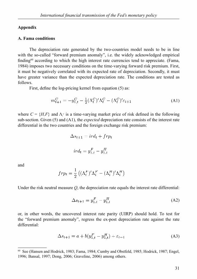
The depreciation rate generated by the two-countries model needs to be in line with the so-called “forward premium anomaly”, i.e. the widely acknowledged empirical finding60 according to which the high interest rate currencies tend to appreciate. (Fama, 1984) imposes two necessary conditions on the time-varying forward risk premium. First, it must be negatively correlated with its expected rate of depreciation. Secondly, it must have greater variance than the expected depreciation rate. The conditions are tested as follows. First, define the log-pricing kernel from equation (5) as:

(A1)

where C = {H,F} and ΛtC is a time-varying market price of risk defined in the following

sub-section. Given (5) and (A1), the expected depreciation rate consists of the interest rate differential in the two countries and the foreign exchange risk premium:

and

Under the risk neutral measure Q, the depreciation rate equals the interest rate differential:

(A2)

or, in other words, the uncovered interest rate parity (UIRP) should hold. To test for the “forward premium anomaly”, regress the ex-post depreciation rate against the rate differential:

(A3)

60 See (Hansen and Hodrick, 1983; Fama, 1984; Cumby and Obstfeld, 1985; Hodrick, 1987; Engel, 1996; Bansal, 1997; Dong, 2006; Graveline, 2006) among others.


32

Nikola Mirkov

where the slope coefficient of the regression is broadly found to be negative, instead of being 1, as the UIRP would suggest. According to (Fama,1984), the deviations from the UIRP can be expressed as two conditions on the forward premium anomaly. First, there is a negative correlation between the forward risk premium and the interest rate differential:

(A4)

and, secondly, the variance of the foreign exchange risk premium should be higher than the variance of the interest rate differential. Specifically, (Fama, 1984) performs the two following regressions:

and

where Ft and St are the forward- and the spot exchange rate, respectively. He estimates the distance between the coefficients b1 and b2:

to be positive for all the considered currency pairs, from where he concludes that the var(frpt) is larger than var(E(St+1 -St)). Consequently, it follows that var(frpt) is larger than var(irdt) as well61. In other words, most of the variation in the depreciation rate should come from variation in the foreign exchange risk premium. As it is shown in the Section Results, the model satisfies both conditions.

61 See (Fama, 1984) for details.


33


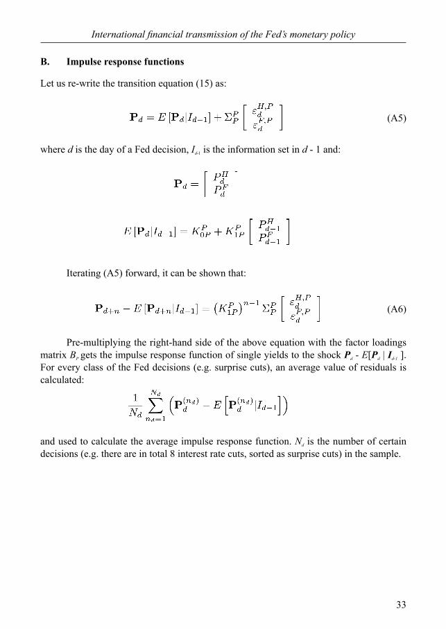
B. Impulse response functions

Let us re-write the transition equation (15) as:

(A5)

where d is the day of a Fed decision, Id-1 is the information set in d - 1 and:

Iterating (A5) forward, it can be shown that:

(A6)

Pre-multiplying the right-hand side of the above equation with the factor loadings matrix BP gets the impulse response function of single yields to the shock Pd - E[Pd | Id-1 ]. For every class of the Fed decisions (e.g. surprise cuts), an average value of residuals is calculated:

and used to calculate the average impulse response function. Nd is the number of certain decisions (e.g. there are in total 8 interest rate cuts, sorted as surprise cuts) in the sample.


34

Nikola Mirkov

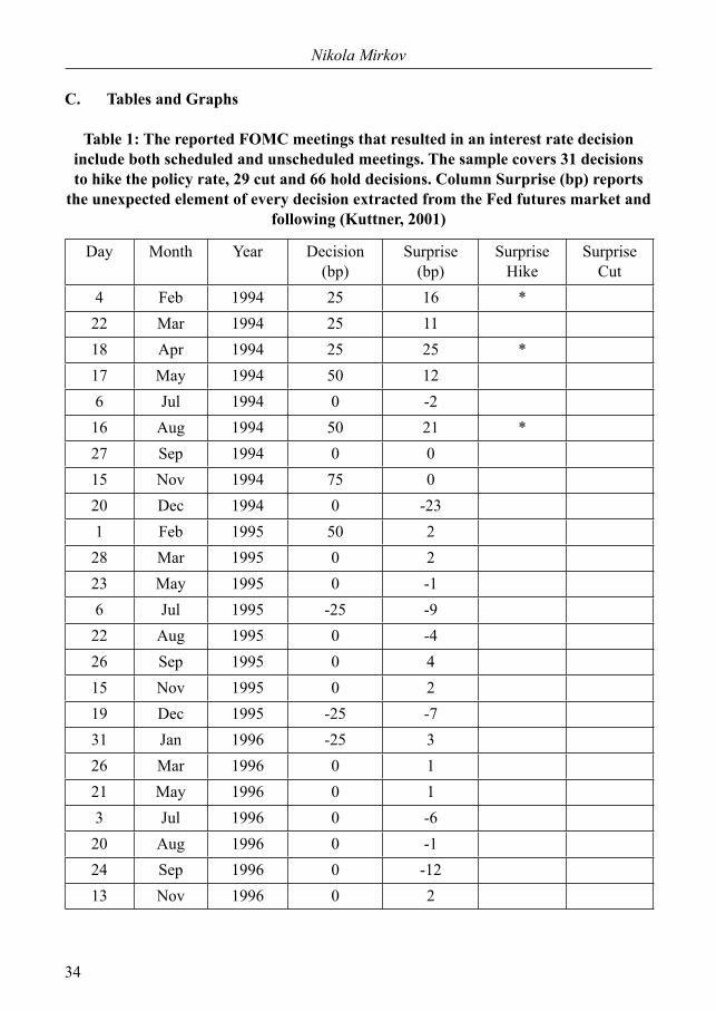
C. Tables and Graphs

Table 1: The reported FOMC meetings that resulted in an interest rate decision include both scheduled and unscheduled meetings. The sample covers 31 decisions to hike the policy rate, 29 cut and 66 hold decisions. Column Surprise (bp) reports

the unexpected element of every decision extracted from the Fed futures market and following (Kuttner, 2001)

Day Month Year Decision(bp)

Surprise(bp)

SurpriseHike

SurpriseCut

4 Feb 1994 25 16 *22 Mar 1994 25 1118 Apr 1994 25 25 *17 May 1994 50 126 Jul 1994 0 -216 Aug 1994 50 21 *27 Sep 1994 0 015 Nov 1994 75 020 Dec 1994 0 -231 Feb 1995 50 228 Mar 1995 0 223 May 1995 0 -16 Jul 1995 -25 -922 Aug 1995 0 -426 Sep 1995 0 415 Nov 1995 0 219 Dec 1995 -25 -731 Jan 1996 -25 326 Mar 1996 0 121 May 1996 0 13 Jul 1996 0 -620 Aug 1996 0 -124 Sep 1996 0 -1213 Nov 1996 0 2


35



Surprise(bp)

SurpriseHike

SurpriseCut

17 Dec 1996 0 05 Feb 1997 0 -225 Mar 1997 25 220 May 1997 0 -92 Jul 1997 0 -119 Aug 1997 0 330 Sep 1997 0 012 Nov 1997 0 -316 Dec 1997 0 -24 Feb 1998 0 031 Mar 1998 0 019 May 1998 0 -51 Jul 1998 0 -218 Aug 1998 0 329 Sep 1998 -25 415 Oct 1998 -25 -24 *17 Nov 1998 -25 -1222 Dec 1998 0 -43 Feb 1999 0 130 Mar 1999 0 -118 May 1999 0 1030 Jun 1999 25 -824 Aug 1999 25 25 Oct 1999 0 616 Nov 1999 25 1121 Dec 1999 0 122 Feb 2000 25 221 Mar 2000 25 -116 May 2000 50 828 Jun 2000 0 -222 Aug 2000 0 33 Oct 2000 0 215 Nov 2000 0 019 Dec 2000 0 33 Jan 2001 -50 -24 *31 Jan 2001 -50 -520 Mar 2001 -50 -718 Apr 2001 -50 -79 *15 May 2001 -50 -22 *


36

Nikola Mirkov


Surprise(bp)

SurpriseHike

SurpriseCut

27 Jun 2001 -25 921 Aug 2001 -25 -317 Sep 2001 -50 -28 *2 Oct 2001 -50 -146 Nov 2001 -50 -1611 Dec 2001 -25 -730 Jan 2002 0 319 Mar 2002 0 537 May 2002 0 -426 Jun 2002 0 -913 Aug 2002 0 -724 Sep 2002 0 -26 Nov 2002 -50 -1210 Dec 2002 0 029 Jan 2003 0 218 Mar 2003 0 46 May 2003 0 -725 Jun 2003 -25 1112 Aug 2003 0 016 Sep 2003 0 028 Oct 2003 0 -19 Dec 2003 0 128 Jan 2004 0 316 Mar 2004 0 04 May 2004 0 130 Jun 2004 25 -810 Aug 2004 25 721 Sep 2004 25 810 Nov 2004 25 114 Dec 2004 25 02 Feb 2005 25 122 Mar 2005 25 29 *3 May 2005 25 230 Jun 2005 25 29 Aug 2005 25 020 Sep 2005 25 71 Nov 2005 25 113 Dec 2005 25 031 Jan 2006 25 1


37



Surprise(bp)

SurpriseHike

SurpriseCut

28 Mar 2006 25 610 May 2006 25 129 Jun 2006 25 -78 Aug 2006 0 -520 Sep 2006 0 025 Oct 2006 0 -212 Dec 2006 0 -131 Jan 2007 0 09 May 2007 0 128 Jun 2007 0 27 Aug 2007 0 818 Sep 2007 -50 -44 *31 Oct 2007 -25 911 Dec 2007 -25 022 Jan 2008 -75 -63 *30 Jan 2008 -50 -1018 Mar 2008 -75 49 *30 Apr 2008 -25 -725 Jun 2008 0 -45 Aug 2008 0 -316 Sep 2008 0 21

8 Oct 2008 -50 -17coordinated

cut

29 Oct 2008 -50 -10

16 Dec 2008 -75 -35*as

anticipated


38

Nikola Mirkov

Table 2: The table reports the estimated parameters. The standard errors for K1P P

are calculated from the output of an unconstrained VAR(1). The standard errors of the Q parameters are asymptotic standard errors in (·) brackets and bootstrapped

standard errors in {·} brackets

K1PP

US level 0.998 0.004 0.006 0.001 -0.007 0.004(0.002) (0.001) (0.000) (0.001) (0.001) (0.000)

US slope 0.001 0.998 -0.018 -0.001 0.001 -0.003(0.003) (0.001) (0.001) (0.002) (0.001) (0.001)

US curvature 0.001 0.000 0.985 -0.001 0.001 -0.005

(0.012) (0.004) (0.003) (0.010) (0.004) (0.002)UK level 0.004 -0.006 0.026 0.997 -0.004 0.002

(0.002) (0.001) (0.000) (0.001) (0.001) (0.000)UK slope -0.001 0.001 0.009 0.002 0.997 0.018

(0.003) (0.001) (0.001) (0.003) (0.001) (0.001)UK

curvature 0.001 -0.001 -0.006 -0.001 0.000 0.988(0.011) (0.004) (0.003) (0.009) (0.004) (0.002)

LΣPP

US (Home Country)0.131

λ11F,Q (0.082)

0.991 {0.089}(0.005) -0.030 0.035{0.014} (0.053) (0.022)

αF {0.017} {0.005}0.748 -0.025 0.005 0.026

(0.014) (0.029) (0.025) (0.016){0.018} {0.035} {0.012} {0.002} UK (Foreign Country)λ11

Q 0.059 0.002 -0.002 0.0900.997 (0.156) (0.072) (0.065) (0.056)

(0.003) {0.059} {0.021} {0.072} {0.020}{0.003} -0.014 0.010 0.002 -0.016 0.037

α (0.059) (0.033) (0.034) (0.032) (0.022)0.813 {0.010} {0.068} {0.018} {0.091} {0.005}

(0.011) 0.007 0.002 -0.004 0.010 0.004 0.025{0.007} (0.035) (0.024) (0.025) (0.020) (0.024) (0.016)

{0.028} {0.016} {0.041} {0.016} {0.061} {0.007}


39


Table 3: The upper panel of the table reports in-sample mean absolute pricing errors calculated on the entire sample and expressed in basis points. The lower panel

reports the means and the standard deviations of 1-day ahead forecasting errors on different policy days and for the selected 6-month US and the 10Y UK yields. The p-values reported in brackets come from an independent two-sample means

t-test and the levels of significance of .10, .05 and .01 are denoted with *, ** and ***, respectively

Single-country Model6m 2Y 3Y 5Y 7Y 10Y

UK 0.5 2.4 1.3 2.3 1.2 2.0US 0.4 2.4 1.7 1.7 1.0 1.4

Two-country ModelUK

Rank 6m 2Y 3Y 5Y 7Y 10Y2 0.5 2.5 1.4 2.3 1.2 2.14 0.7 3.1 2.0 2.9 1.6 2.7

USRank 6m 2Y 3Y 5Y 7Y 10Y

2 0.3 1.8 1.1 1.5 0.8 1.24 0.3 1.6 1.0 1.4 0.8 1.2

Decisions 6m US 10Y UKmean std mean std

Hikes (31) 0.4 2.2 -1.4 5.2(0.15) (0.31)

- Anticipated Hikes (27) 0.4 2.1 -2.2*** 3.3(0.24) (0.01)

- Surprise Hikes (4) 1.1 3.1 3.6 11.9(0.49) (0.53)

Cuts (28) -4.4** 11.4 0.1 4.6(0.05) (0.44)

- Anticipated Cuts (20) -2.3* 4.8 -0.7 4.0(0.06) (0.77)

- Surprise Cuts (8) -8.1 19.3 2.2 5.5(0.24) (0.18)


40

Nikola Mirkov

Table 4: One-day average changes in the UK yields after different policy actions. The p-values reported in brackets come from an independent two-sample means t-test

6M 1Y 3Y 5Y 7Y 10YAll Decisions (125) -0.4 0.3 0.4 -0.1 0.1 0.0

(0.16) (0.35) (0.22) (0.92) (0.58) (0.82)All Surprises (15) -2.1 0.7 1.6 1.7 2.1 2.4

(0.14) (0.54) (0.20) (0.30) (0.18) (0.15)Hikes (31)

- Anticipated Hikes (27) -0.1 -1.1 -1.3** -1.9*** -1.7** -1.8***

(0.98) (0.11) (0.05) (0.01) (0.02) (0.01)- Surprise Hikes (4) -5.1 0.9 1.2 2.9 3.1 4.6

(0.16) (0.73) (0.65) (0.63) (0.60) (0.49)Cuts (28)

- Anticipated Cuts (20) -0.7 -0.4 -0.1 -0.6 -0.3 -0.2

(0.22) (0.68) (0.99) (0.55) (0.83) (0.90)- Surprise Cuts (8) -1.9 0.9 2.1 1.8 2.2 2.6

(0.32) (0.65) (0.28) (0.32) (0.18) (0.14)

Table 5: One-Day average change in the UK forward term premia in basis points. The estimated premia comes from the two-country model. The p-values reported in

brackets come from an independent two-sample means t-test

6M - 2Y 2Y - 3Y 3Y - 5Y 5Y - 7Y 7Y - 10Y

All Decisions (125) 0.9** 0.8 0.4 0.1 -0.1(0.04) (0.12) (0.44) (0.93) (0.82)

All Surprises (15) 4.2** 5.0** 4.5* 4.0 3.6(0.03) (0.05) (0.09) (0.15) (0.20)

Hikes (31)- Anticipated Hikes (27) -1.4** -1.9*** -1.9*** -1.9** -1.9**

(0.03) (0.01) (0.01) (0.03) (0.05)

- Surprise Hikes (4) 6.8 9.3 9.7 9.5 9.2(0.30) (0.33) (0.36) (0.38) (0.39)

Cuts (28)- Anticipated Cuts (20) 0.4 0.4 0.4 0.3 0.2

(0.70) (0.71) (0.74) (0.79) (0.83)

- Surprise Cuts (8) 4.7** 5.3** 4.4** 3.5 3.0(0.03) (0.02) (0.05) (0.16) (0.26)


41


Table 6: One-Day average change in the UK forward term premia in basis points. The estimated premia comes from the single-country model for the UK. The p-values

reported in brackets come from an independent two-sample means t-test

6M - 2Y 2Y - 3Y 3Y - 5Y 5Y - 7Y 7Y - 10Y

All Decisions (125) 0.9** 0.8 0.4 0.1 -0.1(0.04) (0.12) (0.44) (0.92) (0.83)

All Surprises (15) 4.2** 5.0** 4.5* 4.0 3.6(0.03) (0.05) (0.09) (0.15) (0.20)

Hikes (31)- Anticipated Hikes (27) -1.4** -1.9*** -1.9*** -1.9** -1.8*

(0.03) (0.01) (0.01) (0.03) (0.06)- Surprise Hikes (4) 6.8 9.4 9.8 9.7 9.4

(0.30) (0.33) (0.35) (0.37) (0.38)Cuts (28)

- Anticipated Cuts (20) 0.4 0.5 0.4 0.3 0.3(0.70) (0.70) (0.72) (0.75) (0.78)

- Surprise Cuts (8) 4.7** 5.3** 4.4* 3.4 2.9(0.03) (0.02) (0.06) (0.17) (0.28)

Table 7: One-Day average change in the UK forward term premia in basis points. The premia reaction is estimated on the sub-sample from the beginning of January

1994 until the end of July 2007 and using the two-countries model. The p-values reported in brackets come from an independent two-sample means t-test

6M - 2Y 2Y - 3Y 3Y - 5Y 5Y - 7Y 7Y - 10YAll Decisions (115) 0.7** 0.7 0.4 0.0 -0.2

(0.05) (0.11) (0.39) (0.91) (0.78)All Surprises (12) 3.8** 4.81* 4.5 3.9 3.5

(0.05) (0.08) (0.15) (0.27) (0.35)Hikes

- Anticipated Hikes (27) -1.3* -1.7*** -1.8*** -1.7* -1.7

(0.06) (0.01) (0.01) (0.07) (0.15)

- Surprise Hikes (4) 6.2 9.3 10.4 10.8 10.9(0.24) (0.26) (0.29) (0.32) (0.34)

Cuts (21)- Anticipated Cuts (15) 0.3 0.3 0.3 0.2 0.1

(0.79) (0.79) (0.80) (0.83) (0.86)- Surprise Cuts (6) 2.9 3.4* 2.7 1.9 1.4

(0.14) (0.10) (0.16) (0.40) (0.60)


42

Nikola Mirkov

Table 8: One-Day weighted average change in the UK forward term premia in basis points. The single reactions are weighted with the inverse of the size of policy rate move multiplied by 25, e.g. the reaction to a 75 basis point move is weighted by 25/75. The p-values reported in brackets come from an independent two-sample means t-test

6M - 2Y 2Y - 3Y 3Y - 5Y 5Y - 7Y 7Y - 10Y

All Decisions (125) 0.1 0.2 0.2 0.2 0.2

(0.67) (0.58) (0.54) (0.54) (0.54)

All Surprises (17) 2.5** 3.6* 3.8* 3.9 3.9

(0.05) (0.07) (0.10) (0.14) (0.16)

Hikes (31)

- Anticipated Hikes (27) -1.1* -1.5*** -1.5** -1.4* -1.4

(0.07) (0.01) (0.02) (0.10) (0.20)

- Surprise Hikes (4) 5.6 8.99 10.5 11.4 11.8

(0.29) (0.30) (0.31) (0.31) (0.32)

Cuts (28)

- Anticipated Cuts (20) 0.5 0.7 0.6 0.6 0.6

(0.53) (0.47) (0.46) (0.48) (0.51)

- Surprise Cuts (8) 2.0** 2.4*** 2.1** 1.8 1.6

(0.02) (0.01) (0.04) (0.13) (0.23)


43


Figure 1: The US (Upper panel) and the UK (right panel) yield curves are plotted with the FOMC policy rate decisions to hike (solid lines) or cut (dashed lines) the

Federal funds rate. The grey areas are NBER recessions in the US


44

Nikola Mirkov

Figure 2: The Figure reports the histograms of sizes of the Fed funds rate increases/decreases for different policy actions. The x-axis is expressed in basis points and the

y-axis shows the number of corresponding decisions


45


Figure 3: The Figure reports the histograms of surprise indicator calculated in equation (1) for different policy actions. The x-axis is expressed in basis points and

the y-axis shows the number of corresponding decisions


46

Nikola Mirkov

Figure 4: The Figure reports the decomposition of the UK term premia (solid thick line) to the part driven by the three UK factors (dashed) and US factors (solid thin)


47


Figure 5: The upper panel illustrates the decomposition of the model-implied depreciation rate (solid thick line) to interest rate differential (solid thin line) and foreign exchange risk premium (dashed line). The lower panel plots the modelled depreciation rate (solid line) against the data (dashed line). The data depreciation

rate is annualised and expressed in percentages


48

Nikola Mirkov

Figure 6: The figure reports average impulse response functions of the 6-month (solid line) and the 10-year (dashed line) UK and US yields to a contractionary

(upper panel) and expansionary (lower panel) US monetary policy shocks, together with 90 percent confidence intervals. The confidence intervals are calculated as +/- 1.64 standard deviations of impulse response functions in a group of policy actions

(e.g. hikes)

Hikes


49


Cuts


international ﬁnancial transmission of the fed’s monetary

Documents