international reserves, pooling and macroeconomic
TRANSCRIPT
INTERNATIONAL RESERVES, POOLING AND
MACROECONOMIC STABILITY IN THE ECONOMIC
COMMUNITY OF WEST AFRICAN STATES
BY
Jonathan DastuDANLADI
Matriculation Number: 141643
Bachelor of Science in Economics (Jos)
Master of Science in Economics(Ibadan)
Athesis in the Department of Economics, submitted to the Faculty of the
Social Sciences in partial fulfillment of the requirements for the award of the
degree of
DOCTOR OF PHILOSOPHY
of the
UNIVERSITY OF IBADAN
April 2015

ii
ABSTRACT
International reserves of West African countries rose sharply by 84.3% between 1991 and
2001 and 287.1% between 2001 and 2011. However, due to high macroeconomic
instability in the form of persistent asymmetric shocks, output variability and fiscal policy
distortions, the reserves were inadequate and the countries in the sub-region are
continually faced with the problem of balancing the costs and benefits from reserves
holdings. Previous studies have paid little attention to the factors determining reserves and
the prospect of reserves pooling to reduce the prevalent macroeconomic instability. This
study, therefore, examined reserves determinants and the effects of a prospective reserves
pooling on macroeconomic stability in the Economic Community of West African States
(ECOWAS) subregion between 1981 and 2011, a period within which there was an
availability of uniform time series data on the macroeconomic variables.
The buffer stock model was employed to capture the determinants of reserves (imports,
external debts, government spendings, exchange rates, foreign direct investments, exports
and investment) and the Optimum Currency Area (OCA) asymmetric shock framework
was utilized to evaluate the impact of reserves pooling on macroeconomic stability. Data
were collected from World Bank and International Monetary Fund databases.The fixed
and random effects models in the panel data framework were estimated to capture the
demand and supply determinants of reserves. The impulse response and variance
decomposition in the domain of Panel Vector Autoregression (PVAR) were employed to
estimate the impact of reserves pooling on macroeconomic stability. The PVAR
estimations were undertaken in an ex ante counterfactual analysis and considered reserves
held in an autonomous state as well as under a 60.0% pooling scheme as recommended by
the West African Economic and Monetary Union (WAEMU) as the optimal pooling
arrangement.Diagnostics and robustness tests (reserves optimality, PVAR stability,
residual normality and cointegration tests) were carried out to ascertain the reliability of
the estimates. All estimates were validated at p=0.05.
The statistically significant demand determinants of reserves in the region were imports (-
0.43), external debts (-0.83), government spendings (-0.03) and exchange rates (0.94)
while the supply determinants were foreign direct investments (0.09), exports (0.05) and

iii
investment (0.02) for the Fixed Effect Model. The unbiasedness of the Random Effect
Model was rejected using the Hausman test. Generalised one standard deviation
innovation significantly reduced macroeconomic instability under the pooling scheme
when compared to autonomous state of the individual countries as expressed in the
behavioural models estimated. Percentage instability reduction from reserves pooling were
external debts (22.9%), government spendings (26.8%),investments (54.8%), trade flows
(56.9%), gross domestic product (58.3%) and exchange rates (60.7%).Overall,
macroeconomic instability in the region was reduced by 46.7% when the countries entered
into the 60.0% reserves pooling arrangement.
Adequate reserves holdings through reserves pooling arrangement insulated the
economies of countries in West Africa. Therefore, monetary authorities in the region
should intensify efforts towards the successful establishment of international reserves
pooling.
Keywords:International reserves pooling, Fixed and random effects models, Panel vector
autoregression, Macroeconomic stability, ECOWAS.
Word count: 474

iv
DEDICATION
To God Almighty
Jehovah Jireh
The Lifter of my Head
And
In loving memory of my father
Supol. Danladi Dastu

v
ACKNOWLEDGEMENT
My glorious and eternal indebtedness are for the one and only true God - Jehovah Jireh,
his Son - Jesus Christ and the Comforter – The Holy Spirit by whose favour, direction and
help I started this programme, passed through the system‟s rough roads and finished
victoriously. Oh God, as it is and always, all glory, honour, power and adoration return to
you for without your help, I cannot succeed and with your help, I cannot fail.
Words cannot express my profound and personal gratitude and indebtedness to the
Chairman of my thesis committee, Professor E. OlawaleOgunkola, who because of the
versatility of his distinct, humble and ever-responsive personality despite his tight
schedule and work, laboriously kept a close camaraderie with me and guided me
throughout this mission. His relentless, unalloyed and unflinching commitment and
support has capped this hitherto evanescent aspiration of obtaining this degree into a
substantial and practical reality. In the shaping of my life, his place and worth would
remain irreplaceable and his positive marks indelible. Sir, may God bless you and lift you
to the height of your dreams.May God Almighty will honour you with good health, long
life and prosperity.
My profound gratitude also goes to Dr. OmoAregbeyen who co-supervised this work and
has been very instrumental and passionate in so many ways through out the course of this
work especially through his excellent academic contribution to the thesis and unparalleled
support at various stages of administrative approval. Sir, words cannot express my
appreciation for all that you have done for me in the course of this work. I am very
grateful and I pray that God Almighty will honour you with good health, long life and
prosperity. My special thanks also goes to Dr. M. A. Oyinlola, the third member of my
thesis committee. I want to say a big thank you sir for your time despite your tight
schedules and for your kind attention and insightful comments and contribution
throughout the course of this work.May God Almighty will honour you with good health,
long life and prosperity.
At this juncture, I want to specially acknowledge the contribution of distinguished
Professor IbiAjayi who has been a great mentor and father to me. I deeply appreciate the
love and fatherliness you have showered on me all through these years. You have been

vi
very instrumental to my upliftment and attainment of higher heights. You have been a
great mentor, pillar and porter in the shaping of my life and I will forever be grateful dear
Prof. God Almighty will honour you with good health, long life and prosperity. I want to
also acknowledge the contribution of Emeritus Professor T. A. Oyejide who, despite his
tight schedule, took time to examine my work and make very useful contributions. Sir, I
am very grateful.
My sincere appreciation goes to all my professors and lecturers in the department starting
with my amiable Head of Department Prof.KasseyGarba; and to Prof. P. A. Iwayemi,
Prof. F. Egwaikhide, Prof. Sam Olofin, Prof. A. Adenikinju, Prof. A. Ariyo, DrsA. O.
Adewuyi, F. Ogwumike, O. Olaniyan, A. Bankole, O. Oyeranti, RemiOgun, A.
Folawewo, A. LawansonM. Babatunde, B. Fowowe, A. Aminu, A. Salisu, Sam Orekoya,
AdeniyiTosin. You are all mentors and co-potters in the shaping of my academic life since
my M.Sc. days to this point. The invaluable administrative contribution of the
departmental secretariat is acknowledged: Mrs. Ojebode, Mrs. Adeosun, Mrs.Oladele, Mr.
Ayogu, Mrs. Farotimi, Mr. Terese and Mr. Etim. I say a big thank you.
My gratitude also goes to the African Economic Research Consortium (AERC) for my full
scholarship, sponsorship, and financial assistance at various stages through out the course
of this work.I want to express my gratitude to the Executive Director, Prof. Lemma
Senbet, and all members of the Training and Research Departments: Innocent Matshe,
Tom Kimani, Witness Simbanegavi, Damiano Manda, Catherine Mwalagho, Nancy
Muriuki, Paul Mburu, Ema Ronno, Betha, Elizabeth, IT Engineer Paul, just to mention a
few.This collaborative Ph.D. programme has been a memorable one for meespecially the
rigorous academic training at the Joint Facility for Electives (JFE) at the Kenya School of
Monetary Studies (KSMS) in Nairobi. My gratitude goes to all the imminent professors
that taught me during this programme; my Econometrics Professors: Prof Tomson
Ogwang (Department of Economics, Brock University, Ontario Canada) and Prof. Kidane
(Department of Economics, University of Dare Salam, Tanzania) as well as my
International Economics Professors: Prof. Adugna Lemi (Deparment of Economics,
University of Massachusetts, USA) and Dr. Albert Touna Mama (International Monetary
Fund, Washington, IMF, USA). I am also grateful to AERC for all the conference
vii
invitations for the presentation of this thesis at the proposal and post-field stages in Aruhsa
Tanzania; they where eye-openers into the world of international academia and research. I
am immeasurably thankful and grateful. I am also grateful to Drs. Williams Oral, Rabah
Arezki and Fanniza Domenico at the African Department, International Monetary Fund,
Washington DC, who made useful contributions to the work during my visiting fellowship
to the IMF Headquarters Washington DC USA.
Family is very important to me. At this juncture, I want to specially acknowledge the
contribution and support from all my family members and siblingswho have been pillars
of support through out my life journey Martha Bitrus, Cecilia Tanko, Ishaku Dastu,
Nandom, Success, Longkat, Gloria and my wonderful princess Temple, just to mention a
few. I appreciate the depth of all your love, prayers and support.
How would my study years be without my exhilarating friends Lola, Senami,Omenka,
Sandy, Ify, Alley, Taiwo, Mohammed, Bala, Felix, Osigwe, Chris, Uche, Taofeek, Noah,
Sanusi, Oviku, Saheed, Blessing, Dayo, Yomi,Rifkatu, Jacob, Noble, AK John, Dapo
Bablo, Oni, Nike, Amaka, Ubah, Susan and all the others. I pray that your effort in the
quest for this degree will be bountifully rewarded. You guys have made my study years
simply eventful. May God Almighty make the road to the zenith of your respective
ambitions and aspirations simple and uncomplicated just as you guys have made mine.
GLORY BE TO GOD ALMIGHTY

viii
CERTIFICATION
We certify that this study was carried out under our supervision by Mr. Danladi, Jonathan
Dastuinthe Department of Economics, Faculty of the Social Sciences, University of
Ibadan, Ibadan Nigeria.
_______________________________________________
Prof. E. OlawaleOgunkola
Chairman, Thesis Supervising Committee
B.sc (Econ), M.sc (Econ), Ph.D(Ibadan)
_______________________________________________
Dr. O. O. Aregbeyen
Member, Thesis Supervising Committee
B.Ed (Edu.Mgt/Econs), M.Sc (Econ), Ph.D (Ibadan)
_______________________________________________
Dr. M. A. Oyinlola
Member, Thesis Supervising Committee
B.sc (Econ) (OAU), M.Sc. (Econ), Ph.D(Ibadan)

ix
TABLE OF CONTENTS
TITLE PAGE .................................................................................................................... i
ABSTRACT ..................................................................................................................... ii
DEDICATION ................................................................................................................ iv
ACKNOWLEDGEMENT ................................................................................................ v
CERTIFICATION .........................................................................................................viii
LIST OF TABLES ......................................................................................................... xii
LIST OF FIGURES ....................................................................................................... xiii
CHAPTER ONE: INTRODUCTION .............................................................................. 1
1.1 General Introduction .................................................................................................... 1
1.2 The Problem Statement ................................................................................................ 4
1.3 Objectives of the Study ................................................................................................. 7
1.4 Justification for the Study............................................................................................. 7
1.5 Scope of the Study ........................................................................................................ 9
CHAPTER TWO: RESERVES MANAGEMENT AND ECONOMIC
PERFORMANCE IN THE ECOWAS……………………………………10
2.1 Historical and Contemporary Issues in Reserves Pooling in the ECOWAS ................ 10
2.1.1 Francophone Historical Arrangement (1900-1980) ....................................................... 10
2.1.2 Francophone Contemporary Arrangement (1980 – present) .......................................... 15
2.1.3 Anglophone Historical Arrangement (1900 – 1980) ...................................................... 19
2.14 Contemporary Issues in WAMZ‟s Monetary Integration (1980 – present) .................... 26
2.1.5 Issues in Monetary Integration at ECOWAS-Wide Level (1975 – date) ....................... 28
2.2 ECOWAS Region Macroeconomic Performance and Stability Assessment ................ 30
2.2.1 Foreign Reserves: Months of Imports Cover ................................................................. 30
2.2.2 External Reserves and External Debt ............................................................................. 33
2.2.3 Gross Domestic Product ................................................................................................. 38
2.2.4 Inflation .......................................................................................................................... 43
2.3 Lesson for Macroeconomic Stability ........................................................................... 46
2.4 Lessons from the Euro Zone Crisis for Macroeconomic Stability ............................... 49
CHAPTER THREE: LITERATURE REVIEW ............................................................ 51
3.1. Review of Theoretical Literature ............................................................................... 51
3.1.1. Theory of Demand for Reserves: The Buffer Stock Theory ......................................... 51
3.1.2. The Theory of Optimum Currency Area (OCA) ........................................................... 55
3.1.3 The Theory of Clubs ...................................................................................................... 60
3.2 Benefits and Costs of Reserves Pooling ....................................................................... 68
3.3 Methodological Review ............................................................................................... 70
3.4 Empirical Review ....................................................................................................... 74

x
CHAPTER FOUR: THEORETICAL FRAMEWORK AND METHODOLOGY ......... 81
4.1 Theoretical Framework .............................................................................................. 81
4.1.1. Theory of Demand for Reserves: The Buffer Stock Model .......................................... 81
4.1.2 The OCA and Asymmetric Shock Model ...................................................................... 85
4.2 Methodology ............................................................................................................... 92
4.2.1 Model 1 .......................................................................................................................... 92
4.2.2 Model 2 .......................................................................................................................... 94
4.3 Estimation Techniques ............................................................................................... 97
4.4 Data Type and Sources ............................................................................................... 99
CHAPTER FIVE: EMPIRICAL ANALYSIS .............................................................. 100
5.1 Data Diagnostics ....................................................................................................... 100
5.1.1 Summary Statistics ....................................................................................................... 100
5.1.2 Panel Unit Root Test .................................................................................................... 102
5.1.3 Cointegration Test ........................................................................................................ 104
5.2 Fixed Effects and Random Effects Models for Determinants of International Reserves
in ECOWAS ................................................................................................................... 108
5.3 Vector Autoregressive Analysis ................................................................................ 114 5.3.1 VAR Stability Condition Check Using the Inverse Roots of AR Characteristic
Polynomial ............................................................................................................................ 114
5.3.2 VAR Residual Tests for Autocorrelations ................................................................... 115
5.3.3 VAR Lag length Selection Criteria .............................................................................. 119
5.3.4 VAR Residual Residual Normality Tests..................................................................... 121
5.3.5 Impulse Response Analysis.......................................................................................... 123
5.3.6 Variance Decomposition .............................................................................................. 142
5.4 Analysis of Stability Gained from Reserves Pooling.................................................. 144
5.5 Interpretations .......................................................................................................... 147
5.6 ROBUSTNESS/SENSITIVITY ANALYSIS OF THE OPTIMAL LEVEL OF
INTERNATIONAL RESERVES IN THE ECOWAS .................................................... 149
5.6.1 Assessing the Size and Benefits of International Reserves Pooling ............................ 149
5.6.2 Evaluation of Gains/Losses from Reserves Pooling in ECOWAS .............................. 151
5.6.3 Evaluation of Reserves Pooling in the WAEMU Community ..................................... 167
5.6.4 Evaluation of Reserves Pooling in the non-WAEMU Community ............................. 174
CHAPTER SIX: SUMMARY OF FINDINGS, CONCLUSION AND
RECOMMENDATION ............................................................................................... 182
6.1 Summary and Conclusion ......................................................................................... 182
6.2 Policy Recommendations .......................................................................................... 184
6.3 Limitations of the Study ........................................................................................... 185
xi
REFERENCES ............................................................................................................ 187
Appendices ................................................................................................................... 199
Appendix 1: Variance Decomposition ............................................................................ 199
Appendix 2: Reverse Ordering of Variance Decomposition ........................................... 202
Appendix 3: VAR Estimates ........................................................................................... 205
Appendix 4: Unit Roots Test .......................................................................................... 211
Appendix 5: VAR Residual Heteroscedasticity Tests ..................................................... 214

xii
LIST OF TABLES
Table 2.1. Total External Reserves as % of Total External Debt for WAEMU……...... 27
Table 2.2.Total External Reserves as % of Total External Debt for non-WAEMU..…...27
Table 5.1. Summary Statistics of Macroeconomic Variables Employed in the Study...... 87
Table 5.2. Panel Unit Root Test for the Variables Employed ……………………….…..88
Table 5.3. Panel Cointegration Test ……………………………………..……...…….….90
Table 5.4. Summary of Johansen Cointegration Test Results ……………………....…....91
Table 5.5. Panel Data Analysis of the Reserves Supply Model for ECOWAS……...…..92
Table 5.6. Panel Data Analysis of the Reserves Demand Model for ECOWAS….……..95
Table 5.7. VAR Residual Portmanteau Tests for Autocorrelations ……………………117
Table 5.8. VAR Residual LM test for Serial Autocorrelation…………………………. 118
Table 5.9. VAR Lag Order Selection Criteria ………………………………………….120
Table 5.10. VAR Residual Normality Tests…………………………………………… 122
Table 5.11. Variance Decomposition (Summary) …………….…………………….…. 143
Table 5.12. Analysis of Stability Gained from Reserves Pooling………..……………. .145
Table 5.13. Average Reserves with Different Degrees of Pooling for ECOWAS ...….. 153
Table 5.14. Average Reserves Holding and Reserves Variability of ECOWAS ............ 157
Table 5.15. Coverage with and without pooling for ECOWAS Countries……….……. 158
Table 5.16. Gains and Losses from Reserves Pooling for ECOWAS…..……..………. 160
Table 5.17. Summary of Gains/Losses from Reserves Pooling for ECOWAS .……… 164
Table 5.18. Optimal Reserves Gains and Loss for ECOWAS (at 60% partial pool).….. 166
Table 5.19. Coverage without and with Pooling for WAEMU Countries ……...….….. 168
Table 5.20. Gains and Losses from Reserves Pooling for WAEMU……..………...….. 170
Table 5.21. Summary of Gains & Losses from Reserves Pooling under different Degrees
of Pooling for WAEMU (US$ Million)…………………………..……………………. 172
Table 5.22. Optimal Reserves Gains & Losses for WAEMU (at 60% Partial Pool)..…. 173
Table 5.23. Coverage without and with Pooling for non-WAEMU Countries……….... 175
Table 5.24 Gains and Losses from Reserves Pooling for non-WAEMU………..……... 177
Table 5.25 Summary of Gains/Losses from Reserves Pooling for non-WAEMU…….. 179
Table 5.26 Optimal Reserves Gains and Losses for non-WAEMU (at 70% Partial Pool)
…………………………………………………………………….……………………..180

xiii
LIST OF FIGURES
Figure 2.1 WAEMU Total Reserves and Change in Reserves (1960-1980)……….…… 13
Figure 2.2 WAEMU Total Reserves and Change in Reserves (1981-2012) …………… 18
Figure 2.3 Non-WAEMU Reserves and Change in Reserves (1923-1950) ……….……. 23
Figure 2.4 Non-WAEMU Reserves and Change in Reserves (1980-2012) ………….…. 25
Figure 2.5 Trends of Foreign Reserves for WAEMU (Months of Imports Cover) …….. 31
Figure 2.6 Trends of Foreign Reserves for non-WAEMU (Months of Imports Cover) ...
32Figure 2.7 Total External Reserves as % of Total External Debt for the ECOWAS
Countries (except Nigeria) ……………………………………………………………… 37
Figure 2.8 GDP Per Capita (Current US$) for WAEMU ………………………………. 39
Figure 2.9 GDP Per Capita (Current US$) for non-WAEMU ……………………….…. 40
Figure 2.10 GDP Per Capita (Current US$) for the Countries combined……….….…… 42
Figure 2.11 Inflation (Percentage of Consumer Prices) for WAEMU…………….….…. 44
Figure 2.12 Inflation (Percentage of Consumer Prices) for non-WAEMU………..……. 45
Figure 2.13 Change in Reserves for WAEMU and non-WAEMU (1982-2012)……..…. 48
Figure 5.1 VAR Stability Test………………………………….…………………...….. 116
Figure 5.2 Response of Government to Innovation from Unpooled Reserves……..….. 124
Figure 5.3 Response of Government to Innovation from pooled Reserves………..……125
Figure 5.4 Response of Investment to Innovation from Unpooled Reserves……..…… 127
Figure 5.5 Response of Investment to Innovation from pooled Reserves…………..…. 128
Figure 5.6 Response of Trade Flows to Innovation from Unpooled Reserves……..….. 130
Figure 5.7 Response of Trade Flows to Innovation from pooled Reserves………..…... 131
Figure 5.8 Response of GDP to Innovation from Unpooled Reserves…………..…….. 133
Figure 5.9 Response of GDP to Innovation from pooled Reserves………..…………... 134
Figure 5.10 Response of External Debt to Innovation from Unpooled Reserves ….….. 137
Figure 5.11 Response of External Debt to Innovation from pooled Reserves.…….…... 138
Figure 5.12 Response of Exchange Rate to Innovation from Unpooled Reserves ….… 140
Figure 5.13 Response of Exchange Rate to Innovation from pooled Reserves……..…..141
Figure 5.14 Average Reserves with Different Degrees of Pooling for ECOWAS Countries
(US$ Billions)………………………………………………………………….….…… 154

xiv

1
CHAPTER ONE
INTRODUCTION
1.1 General Introduction
International reserves1 are the stocks of foreign exchange or savings acquired for
international transactions between the residents of a country and the rest of the world
during a given period of time.2 The net of the receipts and expenditures of foreign
exchange adds or depletes the stock of reserves depending on whether a net inflow or net
outflow has occurred. Where receipts exceed expenditures, an accretion to external
reserves is recorded. On the other hand, reserves are depleted when the reverse is the case.
Against the backdrop of increasing globalisation, acceleration of international capital
flows and financial markets integration, the subject matter of international reserves is
receiving renewed global interest among policymakers and academicians. Reserves
accumulation plays a significant role as a buffer stock against external and unforeseen
shocks or volatilities. This precautionary reason suggests that reserves be held by the
monetary authorities to cushion external shocks that may not be easily predicted or
envisaged. Having such reserves is of upmost significance as the impact of these external
shocks are mitigated while remedial measures are put in place to stabilise the foreign
exchange market and strengthen the external sector with some more permanent safeguard
measures.Further, external obligations are often settled in foreign exchange, thus, the
stock of reserves becomes very important as a source of financing external imbalances
such as payment for imports and settlement of external debt. External reserves are often
deployed when the market clearing exchange rate undershoots or overshoots the
1 Otherwise known as external reserves, foreign exchange reserves, or simply reserves (as will be used
interchangeably in this study).
2 The International Monetary Fund (IMF) (2003) defines international reserves as “consisting of official
public sector foreign assets that are readily available to, and controlled by the monetary authorities, for
direct financing of payment imbalances, and directly regulating the magnitude of such imbalances, through
intervention in the foreign exchange markets to affect the currency exchange rate and/or for other purposes.”

2
levelconsistent with the attainment of the prime goal of macroeconomic stability as well
as for the defense of the value of the local currency. In addition, part of the external
reserves of a nation can be utilised to take advantage of high returns on investment
opportunities especially when substantial and the country‟s portfolio of assets is well
diversified. External reserves reduce a country‟s risks in the international market by
reducing borrowing cost (Abeng, 2007). Besides, reserves can be accumulated as indirect
“collateral” for guaranteeing foreign direct investment (FDI).
While reserves accumulation is desirable, there are costs associated with the holding of
external reserves; these include sterilisation cost, opportunity cost andbalance sheet risks
(Abeng, 2007). Sterilisation cost refers to the fiscal cost, which is the difference between
the returns the monetary authority earns on external reserves investment and interest
payments on government borrowing. That is a fiscal cost is incurred if the rate of returns
on the former is less than the cost of the latter. The opportunity cost of reserves
accumulation is theforegone alternatives such as the development of infrastructure in the
country or its investment in global financial markets abroad. Moreover, if external
reserves create a false sense of security, it is often the case that the incentive and
competency of the authorities to tackle difficult reforms and shocks may be undermined.
Further, the rapid accumulation of external reserves may also lead to complications in the
formulation of monetary policies especially under a flexible foreign exchange rate regime.
Most countries are usually faced with the issue of balancing these benefits and costs of
reserves accumulation. One of the ways to balance these benefits and costs is through a
reserves pooling arrangement among countries in the same region. Belonging to a regional
reserves pooling scheme can be beneficial. It is helpful in emergencies and is expected to
expand the capacity of the countries in the region to tackle any financial crisis, as well as
contribute substantially to the economic stability of the region. With such a reserve pool in
place, timely financial assistance can be offered any crisis-stricken economy in the pool
and it will also prevent further collapse as well as spread to other economies within the
pool (Fafchamps et al, 2007). In the absence of reserve pooling, countries use their
reserves to self-insure themselves first against external shocks, without taking into account
the effect of their actions on the welfare of their neighbours or trading partners. Notably,
regional reserves pooling arrangements can internalise this externality and thereby

3
increase welfare for all countries involved (Ben-Bassat and Gottlieb, 1992; Jeanne and
Ranciere, 2006).
Further, reserves pool can improve risk-sharing by transferring endowments across
countries in advance of the production stage (Basu et al, 2010; Callen et al, 2009). As
noted in Cole and Obstfeld (1991), interactions among countries through trade offer some
risk-sharing properties through fluctuations in the terms of trade. The transfer of
endowments can improve upon this setup by impacting on the relative output of different
varieties of goods. Through this, regional reserves pooling internalises the trade
externality. According to Aizenman and Lee (2006), regional reserves pooling can serve
as a commitment device that can help prevent the negative externalities that exist in an
environment where countries are engaged in a game of competitive devaluation. In
addition, the pooling of reserves improves the diversification of idiosyncratic country
endowment risk. The benefits of diversification are greater when the trade externality is
internalised within a regional pool (Basu et al, 2010).
Apparently, there are costs associated with a country participating in the pooling of
reserves with other members of its region. These costs include the following: first, the loss
of independent monetary policy; in this regard, it can be recalled that it was earlier stated
that external reserves are often deployed when the market clearing exchange rate
undershoots or overshoots the level consistent with the attainment of the prime goal of
macroeconomic stability. Reserves are often used for the defense of the value of the local
currency. This suggests that foreign reserve is a potent tool in the hands of the monetary
authorities of any economy. Thus, if a country does not have access to its own reserves,
having ceded same to a union, the country becomes impotent and dependent on the
monetary policy coming from the central monetary authority of a union she belongs to.
Also, the economy loses seigniorage, a source of revenue to the government (Ricci, 2008;
Abeng, 2007).
Second, asymmetric shocks - which encapsulate exchange rate variability, output
variability, terms of trade as well as variation in consumer price index (CPI). The cost of
pooling increases significantly within a group of countries in a region when they face
these shocks asymmetrically. Third, fiscal policy distortions - a country belonging to a

4
pool becomes “responsible” for the management of the economy of other members. When
a member is faced with any macroeconomic perturbation beyond its control, other
members in the union are obliged to provide support and bail the ailing economy to reduce
the risks of spread of the “ailment” to other members in the pool. Therefore, the pattern
and size of income/revenue as well as spending of (potential) members becomes an issue
of serious consideration (Masson and Pattilo, 2001;Oyejide, 2012). From the foregoing, it
becomes obvious that countries belonging to a region can enter into a reserves pooling
arrangement to increase resource availability and enhance their overall macroeconomic
stability.
1.2 The Problem Statement
Foreign reserves accumulation has become prominent over the recent years in the
Economic Community of West African States (ECOWAS) especially in this period of
monetary integration and single currency contemplation for macroeconomic stability. The
region has been facing macroeconomic instabilities of varying degrees. This is mainly due
to the fact that the international reserves held by the individual countries in the region are
not adequate to bring about the much-neededstabilisation.Reserves are held as
stabilisation tool by economies in the sense that reserves are used as buffer stock, to settle
external obligations such as imports and external debts as well as intervention in the
foreign exchange market. If there are no reserves, the ability of the monetary authorities to
cushion the adverse effects of external shocks will be seriously undermined. In the
absence of reserves, countries will find it increasingly difficult to settle their international
obligations such as payment for imports and debts. It is a fact that most countries in
ECOWAS are import-dependent and laden with high debt burdens. Instability and
uncertainty prevail in the foreign exchange market of most countries in the region
especially in the West African Monetary Zone(WAMZ), though the West African
Economic and Monetary Union(WAEMU)subregion has achieved some level of stability
in the foreign exchange front due mainly to the operation of a fixed exchange rate.
With regards to macroeconomic instabilities in the region, specific country analysis shows
that the Gambian economy is relatively weak and vulnerable to external shocks due to the
volatile nature of its major sources of growth;groundnut export and tourism. Ghanaian

5
economy is characterised by vulnerable terms of trade shocks as exports performance of
the economy largely depends on cocoa exports and gold, subject to frequent
environmental and global market challenges. In Guinea, the issue of macroeconomic
instability is not different as a weak agricultural base characterises the economy. The
economy depends largely on mining and also on foreign aid. External grant-GDP ratio in
Guinea is one of the highest in the subregion.
In Nigeria, following the period of negative growth in the early 1980s the country adopted
the Structural Adjustment Programme (SAP) in order to stabilise the economy. The major
source of macroeconomic instability arises due to the frequent fluctuation in the prices of
crude oil. This is the mainstay of the Nigerian economy following the neglect of the
agricultural sector in the 1970s. Macroeconomic stability in Sierra Leone remains fragile
due to both internal and external factors. The growth of the economy has been greatly
hampered by the civil war and political crises in 1991 that lasted for about a decade.
During the economic recession, there was no credible economic and monetary policy
instrument designed to tackle its negative impact. Civil unrest and instability also
characterised the Liberian economy. Macroeconomic instability equally persists in the
WAEMU subregion. Meanwhile, the region has attained some relative stability due to the
fact that the countries have been operating under the
CommunatdFinanciereAfricaine(CFA) for a long time.The presumption is that negative
impact of macroeconomic instabilities in the subregion would be substantially reduced if
these countries have ample stockpile of international reserves. However, this is not usually
attainable due to the competing demand for the reserves accumulated by these countries
individually - thus the desirability of a reserve pool.
There is an ongoing debate as to why a government through the monetary authority
accumulates large stock of external reserves in the midst of inadequate infrastructure,
poverty, unemployment, inequality and various economic hardships especially in
developing economies. This fact is vividly captured in the words of President
AbdoulayeWade of Senegal (2000-2012) about the reserves of the Francophone West
Africa: “the African people‟s money stacked in France must be returned to Africa in order
to benefit the economies of the BCEAO (BanqueCentrale des Etats de l‟Afriquedel‟Ouest)
member states. One cannot have billions and billions placed in foreign stock markets and

6
at the same time say that one is poor, and then go beg for money”. This issue is of a
complex nature, especially in the West African context, given that the trade-off between
external reserves accumulation and the de-accumulation of same is equally of a
complicated nature too.
Although it is desirable that external reserves be depleted and be injected into the
economies to develop and maintain infrastructure, eradicate poverty, create employment,
and reduce general economic hardships of the populace, it should be borne in mind that a
„large‟ stockpile of external reserves could to be highly volatile and extremely
unsustainable sources. These sources are subject of frequent boom and burst in the
international prices of primary products in the case of most of the countries in the zone
and crude oil prices in the case of Nigeria.3 The prices of these products are often at the
mercy of international price volatilities, which can fall sharplyanytime, as it is the case
and experience during the economic meltdown era. This can lead to macroeconomic
complications not envisagedab initio by these economies. This was the case and
experience of most emerging Asian economies in the 1990s. Thus, quickly depleting
external reserves stocks (especially if it is largely to address domestic issues) may not be
an optimal option after all, as foreign reserves are supposed to be assets or insurance held
against the volatile and uncertain future course of making balance of payments and other
global and unpredictable international transactions.
The puzzle here therefore is that most economies are in dilemma of whether to continue to
accumulate reserves for precautionary purposes (to serves as buffer stock against
unforeseen international macroeconomic shocks) or deplete their reserves (to finance
government purchases and meet several other demands and be at risk of any shock,
instability and vulnerability that may come internally or externally). This problem raises
some pertinent questions that include the following: is there any way in which the
liquidity yields from holding external reserves can be preserved and guaranteed among the
group of countries in the region without the need for the individual countries to
continually accumulate them thereby exposing their economies to external and internal
macroeconomic perturbations? Put differently, can they pool their external reserves and
3Crude oil export, for instance, accounts for more than 90% of Nigeria‟s revenue.

7
reap the benefits of scale economies in the face of the above dilemma? What are the
determinants of international reserves in the region? Would external reserves pooling
arrangement bring about the much anticipated macroeconomic stability in the region? This
thesis seeks to answer these questions.
1.3 Objectives of the Study
The broad objective of this study is to determine the relationship between reserves pooling
and macroeconomic stability in the ECOWAS region. The specific objectives of the study
are to:
a. Estimate the international reserves supply and demand determinants for the region;
b. Evaluate the potential impact of reserves pooling on macroeconomic stability in
the region.
1.4 Justification for the Study
There is relative paucity of evidence in the literature on reserves pooling for the
ECOWAS subregion; particularly covering a rigorous empirical study that attempts to
evaluate the demand and supply determinants of international reserves and examine the
impact of a reserves pooling arrangement. The review of relevant literature on the
determinants of reserves reveals that most of the studies in this area are largely country-
specific thereby requiring country-specific methodologies and analysis while other panel
analyses are done for other regions of the world, not the West African subregion, as in
Elhiraika and Ndikumana (2007), Drummond and Dhasmana (2008), Gosselin and Parent
(2005), Nda (2006), Okorie (2007), Shamsuddeen (2005), Abeng (2007),Obaseki
(2007),Egwaikhide (1999).
Most of these studies have attempted to examine foreign reserves accumulation with some
identifiable implications for economic growth.However, they are inadequate in terms
ofsound theoretical backbone and empirics. Thus, a study that would provide adequate
theoretical framework for understanding and empirically investigate the determinants of
international reserves in the region becomes paramount.
8
The ECOWAS region has been bedeviled by the prevalence of macroeconomic instability
and this study envisages that a reserve pooling arrangement may largely address this
problem. One of the objectives of this study is to determinethe impact of a reserve pooling
arrangement on macroeconomic stability in the region. To the best of the researcher‟s
knowledge, the stability of fundamental macroeconomic variables arising from a possible
reserve pooling arrangement has not been accounted for and properly examined by
previous studies. Thus, an important contribution of this study stems from the evaluation
and analysis of the impact of a reserve pool on macroeconomic stability.
In the area of macroeconomic shocks and stability, the concentration has been on the
wider subject matter of monetary integration and testing for other viable options for a
single currency for the region (Bayoumi and Ostry, 1997; Masson and Patillo, 2001; 2004;
Ogunkola, 2005; Ogunkola and Jerome, 2005; Nnanna et al, 2007; WAMI, 2008; Okafor,
2011). This study addresses the viability of the monetary union through the core subject of
reserves pooling by examining whether countries can gain from a pooling arrangement
and whether this can reduce macroeconomic shocks and enhance macroeconomic stability
in the region. Thus, a study that would provide adequate basis for understanding and
empirically investigating the relationship between international reserves and
macroeconomic stability for the subregion under a pooling and non-pooling arrangement
may be crucial to the region. The expected findings of this study will be useful for policy
formulation and implementation to the monetary authorities that manage the external
reserves of the countries in the sub-region.
In the light of the foregoing, this study aims at extending the frontier of knowledge in
terms of methodological and empirical contributions to the reserves (pooling) literature as
little evidence existson the potential impact of a possible reserves pooling for the
ECOWAS region, especially in the face of increasing contemporary speculations for an
optimum currency area (OCA). In addition, the tools of analysis employed, findings and
recommendations that emerge from the study are expected to enlighten and stimulate other
researchers to further studies.
9
1.5 Scope of the Study
The focus of this study is on international reserves pooling and macroeconomic stability in
the ECOWAS subregion. The countries that make up the ECOWAS are: Benin, Burkina
Faso, Cape Verde, Cote d‟Ivoire, The Gambia, Ghana, Guinea, Guinea-Bissau, Liberia,
Mali, Niger, Nigeria, Senegal, Sierra Leone and Togo. In general, the scope of this study
spans from 1981 to 2011. The choice of the period is largely informed by the availability
of uniform time series data on the variables of interest.

10
CHAPTER TWO
RESERVES MANAGEMENT AND ECONOMIC PERFORMANCE IN
THE ECOWAS
2.1 Historical and Contemporary Issues in Reserves Pooling in the ECOWAS
This section provides a historical and contemporary overview of issues with respect to
reserves management and pooling in the West African subregion. The exposition covers
the arrangements as they were in the Francophone and Anglophone regional subdivisions.
2.1.1 Francophone Historical Arrangement (1900-1980)
The creation, maintenance and pooling of reserves in the Francophone African economies
are the products of a long period of French colonialism and the learned dependence of the
African states. According to Busch (2009), limited powers are allocated to the central
banks of most Francophone African countries. There can be no trade policy without
reference to currency; and investment without reference to reserves. Fiscal and monetary
policies as well as reforms for the promotion of economic growth and trade are irrelevant
except with the consent of the French Treasury that rations their funds and guarantees
their convertibility. This system of dependence is a direct result of the colonial policies of
the French government.
According to Hogendorn and Gemery (1988), the sole bank of issue for French West
Africa was founded in 1901. It was called the Banque de l'AfriqueOccidentale (BAO).
The currency circulated by the Bank, Franc, was at par with the French Franc until 1945 at
which time; the CFA (Colonies Francaisesd'Afrique, later
CommunautdFinanciereAfricaine) Franc was established. In the immediate post-war

11
period after the signing of the Bretton Woods Agreement in July 1944, the French
economy urgently needed to recover from the several disasters of the Second World War.4
Following the devaluation of the French Franc, it was naturally expected that the currency,
which was also circulating in Francophone Africa, would also be devalued. Instead,
France decided to create a new currency for its African colonies on 26 December 1945.
The newly created CFA was however not devalued but overvalued. In deciding to
overvalue the new currency, the CFA zone economies were effectively excluded from the
international market as their products became too expensive on the competitive global
market. There remained only one market for the CFA zone, and that was France their
colonial master. This enabled Metropolitan France to appropriate to itself the raw
materials needed for its post-war and young industries. The colonies were tied hand and
foot to serve metropolitan France as other markets closed their doors to their expensive
products. Thus through the new CFA currency, France economically re-colonise its
African colonies that had earlier been cut off from Paris as a result of the War.
The French allowed the independence of its colonies but at the price of a strict continuing
control over their economies after SekouToure's of Guinea voted "no" in the 1958
referendum to create a Franco-African Community that stopped short of total
independence. Soon after, they agreed at independence to be bound by the “Pacte
Colonial”. The result of which was an agreement signed between France and its newly-
liberated African colonies which locked these colonies into the economic and military
embrace of France. This Colonial Pact is the genesis of the institution of the CFA franc
and the Franc zone. This pact also created a legal mechanism under which France obtained
a special place in the political and economic life of its colonies. The pact also maintained
the French control over the economies of the African states as well as it took possession of
their foreign currency reserves (Busch, 2009).
4To assist in this process, it set up the first CFA amongst its African colonies to guarantee a
captive market for its goods. Also, France needed the currencies of its colonies to support its
competitiveness with its American and British competitors.

12
Under the CFA zone, there are two prominent monetary unions: The West African CFA
zone, known as WAEMU or UEMOA which comprises of Benin, Burkina Faso, Côte
d‟Ivoire, Guinea Bissau, Mali, Niger, Senegal and Togo and the Central African CFA
zone5, comprises Cameroon, Central African Republic, Chad, Equatorial Guinea, Gabon,
and the Republic of the Congo.6 The WAEMU and CAEMC zones each have a common
central bank: BanqueCentrale des Etats de I‟Afrique de l‟Ouest(BCEAO) and Banque des
Etats de l‟AfriqueCentrale (BEAC), respectively. WAEMU has a common pool of
reserves which under an agreement are kept with and managed by the French Treasury
(Ebi, 2002). Figure 2.1 shows the total reserves of the WAEMU countries and the change
in reserves within the period. A careful look shows that the reserves fluctuate significantly
with the lowest in 1977 where reserves fell from $725.1 million to $445.1 million,
representing a deficit amounting to $280 million.
The WAEMU CFA franc was originally pegged at 100 CFA for each French franc but,
after France joined the European Community, Euro zone, at a fixed rate of 6.65957 French
francs to one Euro, the CFA rate to the Euro was fixed at CFA 665,957 to each Euro,
maintaining the 100 to 1 ratio. It is important to note that it is the responsibility of the
French Treasury to guarantee the convertibility of the CFA to the Euro. The monetary
policy governing such a diverse aggregation of countries is uncomplicated because the
French Treasury in fact, operates it, without reference to the central fiscal authorities of
any of the WAEMU states.
5known as CAEMC
6They operate almost identically

13
Figure 2.1. WAEMU Total Reserves and Change in Reserves (1960-1980)
Source: Author’s Computation, WDI (2011)
-400
-200
0
200
400
600
800
Reserves ($ Million) Change in Reserves

14
Under the terms of the agreement which set up these banks and the CFA, the Central Bank
of each African country is obliged to keep at least 65% of its foreign exchange reserves in
an operations account (or comptedâ operation) held at the French Treasury, as well as
another 20% to cover financial liabilities.
The CFA central banks also impose a cap on credit extended to each member country
equivalent to 20% of that country public revenue in the preceding year. Even though the
BCEAO has an overdraft facility with the French Treasury, the draw-downs on that
overdraft facility are subject to the consent of the French Treasury. The final say is that of
the French Treasury which has invested the foreign reserves of the African countries in its
own name on the Paris Bourse. The central banks of these two zones: the BCEAO for
WAEMU and the BEAC for CEMAC have supranational status.7
This fixed exchange rate regime draws its credibility from monetary agreements with
France, via the Treasury, that guarantees the convertibility of the CFA franc and provide
the central banks an overdraft facility (comptedâ operation) to meet liquidity needs. The
reserves must amount at least to 20% of central bank short-term liabilities. If the reserves
are below this level (or if the comptedâ operation is in debit) for more than one quarter,
the central banks must take corrective measures(interest rate increases, credit rationing,
and seizure of foreign exchange available in the zone).8
The two CFA banks are African, but have no monetary policies of their own. The
countries themselves do not know, nor are they told, how much of the pool of foreign
reserves held by the French Treasury belongs to them as a group or individually. The
earnings on the investment of these funds in the French Treasury are supposed to be added
7For each zone, the reserves of member states are pooled; members have no independent monetary
policy and no possibility of undermining the central bank‟s independence or monetising public
deficits.
8More than 80% of the foreign reserves of these African countries are deposited in the operations
accounts controlled by the French Treasury.
15
to the pool but no accounting is given to either the banks or the countries of the details of
any such changes. The limited group of high officials in the French Treasury, who have
knowledge of the amounts in the operations accounts where these funds are invested,
whether there is a profit on these investments, are prohibited from disclosing any of this
information to the CFA banks or the central banks of the African states. Therefore, at all
times, no decision can be approved to be valid at the BEACO without the French. France
is, therefore, in a position to block any major decisions taken by these banks. So if a
decision by any of the countries within the zones does notfavour and tally with French
interests, the French administrators have the power to block it (Busch, 2009). The way
these central banks function, therefore, legalise and perpetuate the direct intervention of
France inthe CFA zone economies. Even the appointment of the governor of the BEACO,
must be approved by Paris which seeks to ensure that the governor is malleable and ready
to dance to French tunes. This makes it impossible for these Francophone West African
members to regulate their own monetary policies. The most inefficient and wasteful
countries are able to use the foreign reserves of the more prudent countries without any
meaningful intervention by the wealthier and more successful countries (Busch 2009).
2.1.2 Francophone Contemporary Arrangement (1980 – present)
With the signing of a new UMOA treaty in 1973, a new cooperation agreement and a new
operational account convention with France were put in place. A new administrative
structure was put in place, which includes the appointment of AdoulayeFadiga as the first
African governor of the BCEAO as well as the transfer of the headquarters of the BCEAO
from France to Dakar, Senegal. In line with its mission, the BCEAO decides on an annual
basis the total amount of currency to be allocated to each member country. In order to do
this, it takes into account movements in production prices, the monetary situation, and the
state of each country‟s balance of payments as well as the other objectives that had been
set by the UEMOA council of ministers as regards external assets and liabilities held by
the union and by each member state (Fajana, 2011).In 1994, with the devaluation of the
CFA Franc, the Union became the West African Economic and Monetary Union

16
WAEMU or UEMOA (in French). Nothing much has changed over time in the WAEMU
especially in term of operational issues.9
The role of the BCEAO in the contemporary setting has not changed much over the years
compared to the early years. Its major function in the contemporary setting includes
serving as the bank where the pooled reserves of the zone are deposited. The reserves
were held in the operations account at the French Treasury. Subsequently, there was an
amendment to this practice which made it possible for BCEAO to invest part of its foreign
exchange reserves in certain types of negotiable bonds, which matured within two years
and was issued by international financial institutions of which all BCEAO states were
members. After the amendment, member states were investing part of their foreign
reserves in short term bonds which was issued by the World Bank. Also, the BCEAO still
performs some credit creation functions within the framework of rediscount ceilings,
which are the principal means used to extend both short term and medium term credit.10
Short term credit was granted was by the BCEAO for periods not exceeding six months
but could be extended for an additional five months for financing public contracts while
medium term credits were granted for periods not exceeding five years (Fajana, 2011).
Figure 2.2 shows the reserves of the WAEMU in the contemporary era as well as the
change in the reserves for the period 1981 to 2012. It can be observed that the reserves
maintained a steady rise through to the end of the period. The only observable fluctuation
in the trend of the reserves of the WAEMU is seen around the period of the global and
financial crisis witnessed around the late 2000s.
According to William, Polius and Hazel (2001), the institutional framework in the CFA
franc zone makes it possible for member states to use pooled reserves in counterpart of
local currency. Within these arrangements, fiscal imbalances of member countries, unless
9The French Treasury guaranteed the convertibility of the CFA Franc.
10
Short term credit was extended in the form of rediscount of short term paper and temporary
advances against private and government paper as well as direct advances secured by either gold
or foreign exchange and securities acceptable to BCEAO.

17
funded by other members within the pool, can result in a decline in the foreign assets of
the respective central banks. Each central bank is obliged to maintain 65% of its official
reserves in the operations account as a counterpart to the guarantee of the French treasury.
For the usage of the reserves, each country draws down its own account of pooled and
unpooled reserves in the first instance and then may use other country‟s pooled reserves
once these are fully drawn down as there is no statutory limit on a member country's use
of another's reserves. When the reserves of an individual country are exhausted, an alarm
is not raised at this instance since that country can still benefit from the pooled reserves of
other countries but an alarm is raised and a crisis management scheme takes over when the
BCEAO reserves fall below the prescribed threshold.

18
Figure 2.2. WAEMU Total Reserves and Change in Reserves (1981-2012)
Source: Author’s Computation, WDI (2011)
-2000
0
2000
4000
6000
8000
10000
12000
19
81
19
82
19
83
19
84
19
85
19
86
19
87
19
88
19
89
19
90
19
91
19
92
19
93
19
94
19
95
19
96
19
97
19
98
19
99
20
00
20
01
20
02
20
03
20
04
20
05
20
06
20
07
20
08
20
09
20
10
20
11
20
12
Reserves ($million Change in Reserves

19
Two institutional factors contribute to some members in the CFA franc zone using more
resources from the pool than they contribute. First, the French treasury's guarantee of the
central banks' operations account relieves them of having to monitor their reserves
position and credit creation using the fiscal borrowing and sight liabilities rules. Second,
the fact that each country has unrestricted access to the pooled reserves of other members
makes governments more inclined to monetize budget deficits. Countries are also less
inclined to monitor their balance of payments situation. This feature of the arrangement is
one of the institutional problems in the formation of clubs that attempts to mitigate the
costs of bargaining among members. In essence, it allows for an upper and lower limit
within which bargaining in the form of access to the common pool of reserves can occur.
According to Fajana (2012), by contemporary definition, the UEMOA can be seen as a
complete monetary union. Not only is there complete pooling of monetary reserves and
the issuing of a common currency among the participating countries, there is also a
substantial integration of their financial markets and obstacles to internal payments and
transfers are removed. Furthermore, UEMOA through the operations of BCEAO
facilitates the coordination of other economic policies of its members with regard to trade
and economic development in general. The French Treasury guarantees the reserve pool
available in the CFA franc zone. This ensures a degree of credibility of the regional
financing facilities.
2.1.3 Anglophone Historical Arrangement (1900 – 1980)
The role of international reserves became prominent in the colonial monetary system in
British West Africa when the West African Currency Board (WACB) was established in
1912. According to Hopkins (1970), the Board presided over a monetary system, which
was effectively an extension of that of the British system. The currency of the colonies
was visually distinct and was backed by its own reserves, but it was held at parity with and
was readily convertible into the currency of the ruling power, the British Sterling.
The currency boards served three main purposes: the issue of local currency, the
maintenance of its convertibility into sterling at a known rate of exchange, and the
provision of some revenue to the colonial governments, through their shares in the profits

20
from the coinage, and from the investment of the Board's assets (Abdel-Salam, 1970).The
currency board was more of large-scale money changing centre, also overseeing the
reserves of the colonial British West Africa, investing the reserves of the colonial currency
as well as the distribution of the profits derived from these investments and the
seigniorage on coins issued for the British West Africa. It can be seen that the role of the
Board in terms of reserves pooling was not pronounced when compared to the
Francophone zone.11
.
Hogendorn and Gemery (1988) observe that the currency notes and coins issues of the
WACB were also made against exports. The Board issued its coins and currency at Accra,
Bathurst, Freetown, and Lagos, against the exact equivalent in sterling lodged with the
Board in London. However, WACB notes and coins were convertible into sterling on
payment of a service charge. The convertibility was guaranteed only on presentation at the
West African centres, with the payment of sterling made in London. It was the annual
export of produce that in effect provided the wherewithal for the new West African coins
and currency. Only when exports exceeded commodity imports (plus or minus any capital
transactions in the balance of payments) would there be earnings of sterling or other
currency convertible into sterling that could be lodged with the WACB as a backing for
the West African notes and coins issues.
The sterling acquired as a reserve was invested mainly in UK national and local
government bonds and securities; in practice the WACB did not buy the bonds or
securities of its constituent territories. The result was such that the reserves of the currency
board were largely unavailable for development purposes in the area where the original
saving had been made to acquire the new transactions balances. The amount of currency
issued was substantial; £10 million was reached in 1923, £15 million in 1928, just under
£20 million in 1937, £25 million in 1944, £40 million in 1947, and £67 million only two
years later in 1949. Against these sums the Board's reserves, held in sterling balances were
11
Criticisms levelled against the currency board system were being operationally rigid and
institutionally limited
21
invested in the UK. The result was a loss to West Africa of most of the seigniorage on the
issue of currency.12
Reasons for the marginal return included the following: first, the investments were largely
short and medium term, with interest rates lower than on long-term bonds. For instance,
44% of the WACB's invested reserves carried maturities of less than 5 years in 1950; 75%
had maturities less than 10 years; second, no payout of interest was made to the
constituent territories unless reserves were at or above the target figure of 110%. Third,
the Board covered its operating costs, including the printings of paper notes, the minting
of coin, transport, distribution, and administrative expenditures from the interest earned on
reserves. At 19% of interest income in 1950 (and 86% of that due to the manufacturing
costs of currency) these costs were not negligible. These operating costs were not,
however, excessive and would have had to be met in any case by any substitute system. It
was for the first two reasons, primarily, that interest returns were a weighted average of
only 1.22%between 1923 and 1950, at a time when the average yield on British consoles
was nearly three times higher at 3.60% (Hogendorn and Gemery, 1988).
Figure 2.3 shows WACB reserves and the annual change in reserves without subtraction
for expenses. Thus, during this period only a small fraction of the available seigniorage
was transferred back to the colonial territories as interest income on the invested reserves.
The seigniorage losses to West Africa involved with the WACB currency were thus in
concept closely akin to those involved with the earlier West African moneys, in that they
all represented full-bodied currencies with a pound-for-pound outlay of exports equal in
value (or even greater considering the WACB's 110% reserves) to the entire value of the
money supply. With the pre-colonial moneys, the outlay closely matched real resource
costs including transport in the production and delivery of the currency. With the colonial
notes and coins, the outlay was a transfer to the colonial power of the seigniorage involved
in the money issue.
12This loss was in part offset by the distributions to the colonial governments of interest on the
invested reserves, which was very small.

22
The colonial monetary system was not without its advantages. It assisted the development
of trade between West Africa and the United Kingdom, while at the same time relieving
the mother country of all responsibilities towards the currency of the colonies. The
currency board system gave stability and confidence to the colonial currency by linking it
with the Sterling; it practically eliminated the risk of inflation by providing strict control
over the currency issue. It also corrected any tendency towards the accumulation of
deficits in the balance of payments by ensuring that the local currency and sterling were
automatically convertible, provided some additional revenue that had not been available to
the colonies before 1912. However, the major drawback associated with the colonial
monetary system was that it tended to impede structural economic change since additional
domestic trade could only be financed when the balance of payments was favourable.

23
Figure 2.3. Non-WAEMU Reserves and Change in Reserves (1923-1950)
Source: Hogendorn and Gemery (1988)
-20
-10
0
10
20
30
40
50
60
70
80
19
23
19
24
19
25
19
26
19
27
19
28
19
29
19
30
19
31
19
32
19
33
19
34
19
35
19
36
19
37
19
38
19
39
19
40
19
41
19
42
19
43
19
44
19
45
19
46
19
47
19
48
19
49
19
50
Reserves (£ Million) Change in reserves

24
With the attainment of political independence, each of the former British West African
colonies opted to establish their own monetary system managed by a central bank. The
WACB inevitably became redundant (Hopkins 1973).From the foregoing exposition, the
functions of the currency board were more of issuance of the local currency and money
changing activities. Reserves pooling in the WACB area of West Africa was in the form
of sterling balances which constituted a net loan to Britain from Africa (that is Britain
guaranteeing convertibility of reserves).13
That being the case, it was preferable to invest
in securities with higher yields, which could be readily mobilised into liquid assets
(Abdel-Salam,1970).
From figure 2.4, the reserves position of the non-WAEMU region started soaring from the
period 1997 and reached its peak around 2007 before recording a steady decline. This can
largely be attributed to the global and financial crisis of 2007 where the reserves of most
countries were largely drawn down in order to cushion the negative effects of the
depression.
13
Reserves pooling was in the form of investment of any country's reserves in the securities of any
other country represents in essence a loan by the former to the latter.

25
Figure 2.4. Non-WAEMU Reserves and Change in Reserves (1980-2012)
Source: Author’s Computation, WDI (2011)
-10000
0
10000
20000
30000
40000
50000
Reserves (£ Million) Change in Reserves

26
2.14 Contemporary Issues in WAMZ’s Monetary Integration (1980 – present)
According to Ebi (2002), it was the failure of the ECOWAS integration process to make
significant progress since its inception in 1975 that motivated the increasing quest for
monetary integration in the Anglophone West African subregion. It was generally felt that
the non-existence of parallel and competing monetary arrangements in the sub-region had
been a major factor militating against the movement towards a single monetary zone.
While the CFA zone has appeared to be a solid arrangement, especially with the backing
of France and the European Union, the countries outside the CFA zone have different
national currencies. The challenge of accelerated integration in the subregion has therefore
fallen more on these latter countries. Consequently, the political commitment to renewed
economic cooperation spearheaded by Ghana and Nigeria since December 1999, and
accepted by Guinea, the Gambia, Sierra Leone and Liberia, made the idea of the fast track
approach to integration a feasible proposition. The idea has crystallised into the formation
of the West African Monetary Zone (WAMZ) with the aim of merging it with the CFA
zone subsequently. At a mini-summit of heads of states and government of member
countries in Bamako in late 2000, the critical decisions were adopted with the intention to
formally establish the WAMZ, with a common central bank, and to introduce a single
currency in the zone by 2003.
According to Tarawalie (2012), The West African Monetary Institute (WAMI) was
established in 2000 and commenced operations in Accra, Ghana in March 2001.14
The
monetary union was scheduled to commence operation in January 2003, after a
convergence process. However, the launching of the union was postponed to July 1st
2005, due to the poor status of macroeconomic convergence. Following the poor
macroeconomic performance by member countries and the non-achievements of the
convergence criteria by the end of 2004, the launch date was further postponed to
December 1st 2009. In January 2009, WAMI prepared a status report on the WAMZ
programme and it was clear from the report that considering the effect of the global
14
It was primarily mandated to undertake policy and technical preparations for the launch of a
monetary union for the WAMZ and the establishment of a WACB.
27
recession on the economies of the member states, it was highly improbable for the
member states to achieve the benchmarks for macroeconomic convergence by December
2009. Based on the recommendation contained in the report, the Authorities once again
postponed the launch date of the second monetary union until (on/before) January 2015.
The mandate of the WAMI was clear: undertaking of policies and technical preparations
for the eventual establishment of the WACB and the introduction of a single currency -
the ECO (Tarawalie, 2012).The country that would be eventually selected by political
considerations to host the headquarters of the WACB (Ghana, Nigeria and Guinea have
applied) was urged to be committed to implementing open sky policy as defined in the
“Yamoussoukro Agreement” (Ebi, 2002).
The primary economic policy objectives of WAMZ are to ensure price stability, sound
fiscal and monetary conditions and a sustainable balance of payments in the member
states. To this end, the WAMZ is enjoined to adopt a regional economic policy for the
zone through effective coordination of member states‟ economic policies, conduct the
regional economic policy in the context of an open market economy and specifically
design and implement common monetary and exchange rate policies in the zone.The
WAMZ is also to put into force a multilateral surveillance system to ensure close
coordination of member states‟ economic policies and sustained convergence of economic
indicators of member states. To undertake this function, the key institutions of the WAMZ
- the Convergence Council, Technical Committee, WAMI and the West African Central
Bank - are to formulate broad guidelines for the design of economic policies of member
states.
It is planned that before the WAMZ would merge with the CFA zone, thus creating the
long-awaited single monetary zone in the sub-region, the member states of the WAMZ are
to comply with some convergence criteria, which will ensure macroeconomic stability and
reasonable growth in the member states. The quantitative primary convergence criteria
are:
single digit inflation rate;
budget deficit (excluding grants) of not more than 4%;

28
central bank financing of budget deficit to be limited to 10% of previous year‟s tax
revenue; and
gross external reserves to cover at least three months of imports.
In addition, there are six secondary criteria, which will be observed in support of the
primary criteria. These are:
prohibition of new domestic debt arrears and liquidation of all existing arrears;
tax revenue to be more than 20% of GDP;
wage bill to be less than 35% of total tax revenue;
public investment to be more than 20% of tax revenue;
maintenance of real exchange rate stability; and
maintenance of positive real interest rates.
2.1.5 Issues in Monetary Integration at ECOWAS-Wide Level (1975 – date)
As stated earlier, ECOWAS was founded in 1975 by all the West African countries.15
The
ECOWAS Monetary Cooperation Programme (EMCP) is the most prominent scheme for
monetary integration in the West African subregion. It was originally scheduled for
between 1991 and 1994, but was extended to the year 2000. It was further extended in
December 1999 to 2004. The specific objectives of the EMCP were to be implemented in
three phases. In the short term, the aim was to strengthen the existing payment mechanism
of the West African Clearing House through the settlement of outstanding payment arrears
in the clearing mechanism; introducing new payment instruments such as the traveller‟s
cheque; introducing a credit guarantee fund facility to support the clearing mechanism;
and removing all non-tariff barriers that tend to restrict the use of national currencies to
effect payments for some current transactions such as hotel bills and air tickets.
In the medium term, the EMCP was expected to achieve limited regional convertibility of
national currencies by removing existing restrictions on their use. In the long run however,
the ultimate goal of the EMCP is the establishment of a single ECOWAS monetary area 15
This includes the Francophone (WAEMU) countries, the Anglophone countries (the Gambia,
Ghana, Guinea, Liberia, Nigeria and Sierra Leone) and Portuguese-speaking Cape Verde.

29
involving the use of a common convertible currency, the establishment of a common
central bank, the pooling of foreign exchange reserves and the negotiation of an external
convertibility guarantee with an appropriate international agency. To facilitate these
objectives, member states were to embark on an economic policy reform programme to
achieve macroeconomic convergence. The policy reform programme was to embrace:
realignment of exchange rates and the adoption of a market-based exchange rate
policy;
removal of exchange control regimes; and
minimising of fiscal deficits and their financing through the rationalisation of
governmentexpenditure and tax reform.
The short-term objectives of the EMCP have not been fully achieved, as exemplified by
the failure to clear the arrears in the clearing house mechanism, the delay in introducing
new payment instruments, the problems with the newly introduced ECOWAS traveller‟s
cheques and the unwillingness of members to remove non-tariff barriers to intraregional
trade and other transactions. The medium- to long-term objectives of the EMCP have also
not been fully attained, leading to the deferral of the establishment of the single monetary
zone.
The need for the second monetary union arose largely as a result of inadequate political
will to forge a strong monetary integration between the CFA zone and the non-CFA zone
under the aegis of the EMCP. The emergence of the WAMZ as a successful monetary
union is thus likely to prevent a total collapse of the EMCP. It may indeed facilitate the
movement towards a single monetary zone in the sub-region since negotiations will take
place between two groups of countries in contrast to the current situation characterised by
uncertainties about the integration process of the sub-region. Even if the eventual merger
of the two monetary zones takes more time to materialise than presently envisaged, the
convergence of the two groups of countries will be less cumbersome than the convergence
of many countries with various currencies. The initiative of the second monetary zone - by
which the Anglophone West African countries would forge a monetary union which
would later merge with the CFA franc zone - is therefore a welcome development. So far,

30
it has been pursued with a reasonable degree of political commitment on the part of the
member states. Apart from the political will demonstrated in the execution of the project,
the economic potential of the zone is a great advantage. The zone accounts for over 70%
of the population of ECOWAS, about 64% of its total GDP, about 66% of total exports
and 60% of total imports of goods and services. Altogether, the zone accounts for about
76% of the gross foreign exchange reserves of the West Africa sub-region. The challenges
facing the establishment of the second monetary zone are daunting. As a result, member
countries need to sustain their current economic policy reforms, implement faithfully the
agreement and statutes of the zone and support the zone‟s institutions, particularly WAMI.
The WAMZ countries are trying hard to comply with the statutes of the zone and operate
strictly on macroeconomic policies that will facilitate the realisation of the WAMZ
convergence criteria and its eventual merger with the existing CFA zone (Ebi, 2002).
2.2ECOWAS Region Macroeconomic Performance and Stability Assessment
The performance of the ECOWAS countries based on some relevant macroeconomic
indicators is assessed. This assessment is pertinent in order to draw lessons for
macroeconomic stability of the region.
2.2.1 Foreign Reserves: Months of Imports Cover
Figure 2.5 shows the trend of foreign exchange reserves of the WAEMU and non-
WAEMU countries in terms of months of imports cover. The months of import cover is a
standard indicator for measuring foreign reserves adequacy in the reserves literature.
As shown in figure 2.5, WAEMU countries experienced varying trends and levels of
foreign reserves holdings in terms of months of imports cover. This is also observed for
the non-WAEMU countries in figure 2.6. In the 1980s, Cape Verde, Ghana and Togo were
the leading countries in terms of reserves hoarding with an average of 5.9 months, 4.4
months and 5 months of coverage respectively. In this period, a rise in demand for
reserves couple with lower demand for imports had driven their capacity to pay for
imports to higher levels than other countries.

31
Figure 2.5. Trends of Foreign Reserves for WAEMU (Months of Imports Cover)
Source: Author’s computation from WDI (2011)
0
1
2
3
4
5
6
7
8
Benin Burkina Faso
Cote d'Ivoire
G-Bissau Mali Niger Senegal Togo
1981-1985
1986-1990
1991-1995
1996-2000
2001-2005
2006-2010
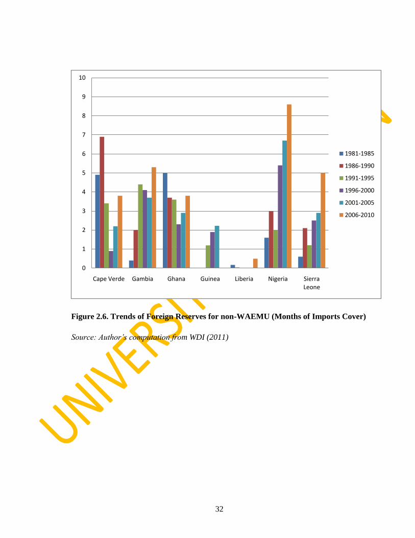
32
Figure 2.6. Trends of Foreign Reserves for non-WAEMU (Months of Imports Cover)
Source: Author’s computation from WDI (2011)
0
1
2
3
4
5
6
7
8
9
10
Cape Verde Gambia Ghana Guinea Liberia Nigeria Sierra Leone
1981-1985
1986-1990
1991-1995
1996-2000
2001-2005
2006-2010
33
More recently, Benin, Guinea-Bissau and Nigeria have been leading other countries of the
region in the hoarding of reserves with an average of 7 months, 6.5 months and 8 months
respectively. These countries have, of late, experience rise in their exports. For Nigeria,
the price of crude oil rose sharply in the early and mid 2000s before the beginning of the
economic recession which started in late 2007. It is observed that on the basis of one of
the WAMZ convergence criteria, only Cote d‟Ivoire is yet to meet its target (on the basis
of at least 3 months of import coverage). A careful consideration of figures 2.1 and 2.2,
show that the WAEMU countries have more stable and adequate amount of reserves in
terms of month of imports cover from reserves over the entire period. The reserves of the
member countries show an even spread compare to the non-WAEMU counterparts with
Guinea and Liberia among the countries responsible for the uneven spread.
2.2.2 External Reserves and External Debt
The ratio of external reserves to external debt in the sub-region is apparently on a
relatively steady increase from their values in the 1980s. This is an indicator of positive
economic performance. For Cape Verde, this ratio was falling until the early 2000s where
it started to rise again. Nigeria‟s case appears to be somewhat phenomenal especially in
the late 2000s as shown in table 2.1. This ratio rose from 51% to 536%. The reserves
position of the country rose astronomically to an unprecedented $60.0 billion as at April,
2008. This positive out-turn in external reserves position was accentuated by a
conglomeration of factors including but not limited to high crude oil prices in the global
market, disciplined fiscal and monetary policy stance and low debt service burden
precipitated by the external debt deal.

34
Table 2.1. Total External Reserves as % of Total External Debt for WAEMU
1981-1985 1986-1990 1991-1995 1996-2000 2001-2005 2006-2010
Benin 3.1 1.8 18.1 23.1 41.6 130.3
Burkina Faso 23.8 37.9 30.6 22.8 27.2 59.8
Cote d'Ivoire 0.3 0.2 0.9 4.6 11.9 22
G-Bissau na 2.2 2.1 3.9 7.1 11.8
Mali 2.6 3.7 10.9 12.9 23.5 61.7
Niger 8.2 14 10.8 3.7 10.2 58.7
Senegal 1 0.7 2.7 9.8 23.9 61.7
Togo 22.2 26.9 15.2 8.1 12.6 32.7
Source: Author’s computation from WDI (2011)

35
Table 2.2. Total External Reserves as % of Total External Debt for non-WAEMU
1981-1985 1986-1990 1991-1995 1996-2000 2001-2005 2006-2010
Cape Verde 68.9 58.9 36.4 9.6 24.3 54
Gambia 1.9 8 22.8 23 15.4 32.2
Ghana 20.6 12.9 12.9 9.5 17.4 na
Guinea na 3.9 4.9 6.3 na na
Liberia 0.8 0.1 0.3 0.0 0.3 8.1
Nigeria 15.9 6.7 6.7 23.4 51.2 536.4
Sierra Leone 1.9 0.7 1.9 3.2 6.5 40.1
Source: Author’s computation from WDI (2011)

36
This made the country‟s debt stock to tumble from an overwhelming $35.9 billion in 2004
to $3.1 billion only in 2007 (Soludo, 2007). Figure 2.7 shows the total external reserves as
% of total external debt for all the ECOWAS countries (except Nigeria). As observed
above, Nigeria is an outlier with respect to this macroeconomic indicator due to its 2006-
2010 average figure which dwarfs all others hence, its exclusion. In this figure, there is an
uneven spread among the countries with Benin, Burkina Faso, Togo and Cape Verde
recording percentages that are above average while the reverse is the case for countries
like Liberia, Sierra Leone, Guinea, Guinea-Bissau and Cote d‟Ivoire where low
percentages are recorded. This reveals that even in the face of reserves pooling, some of
the WAEMU are languishing due to the prevalence of high external debt which is
characterizes most African countries thereby making their reserves to debt ratio to be low.
On the average, it can be observed that most of the countries record significant
improvement with respect to this indicator in the recent periods (2006-2010) with Benin
recording the highest percentage of 131.5%.

37
Figure 2.7. Total External Reserves as % of Total External Debt for the ECOWAS
Countries (except Nigeria)
Source: Author’s computation from WDI (2011)
0
20
40
60
80
100
120
140
1981-1985
1986-1990
1991-1995
1996-2000
2001-2005
2006-2010
38
2.2.3 Gross Domestic Product
An analysis of the GDP per capita of the ECOWAS countries shows varying trends. In
the 1980s countries in the WAEMU zone display elements of poor growth relative to their
non-WAEMU counterparts with an average of $250 per head except for Senegal and cote
d‟Ivoire that were far above this average.This poor performance of WAEMU zone
countries can be attributed to changes in the world economy, persistent current account
deficits and the inability of these economies to adjust. According to Ogunkola (2005), the
growth performance of the CFA zone West African economies did not improve until after
the 1994 devaluation of the CFAF. This slow or negative growth in per capita GDP of the
CFA zone countries was attributed to worsening balance of payments, debt crises,
declining competitiveness and, more importantly, an apparent failure to adjust to the
changes in their environment.

39
Figure 2.8. GDP Per Capita (Current US$) for WAEMU
Source: Author’s computation from WDI (2011)
0
200
400
600
800
1000
1200
Benin B/Faso C/d'Ivoire G-Bissau Mali Niger Senegal Togo
1981-1985
1986-1990
1991-1995
1996-2000
2001-2005
2006-2010

40
Figure 2.9. GDP Per Capita (Current US$) for non-WAEMU
Source: Author’s computation from WDI (2011)
0
500
1000
1500
2000
2500
3000
3500
Cape Verde
Gambia Ghana Guinea Liberia Nigeria S/Leone
1981-1985
1986-1990
1991-1995
1996-2000
2001-2005
2006-2010

41
Over the years, no other country in the sub-region has been able to rival Cape Verde
Island in terms of this economic performance indicator. It has been a stand-alone,
recording an average of about $3000 per head in the year 2000s. This dwarfs that of
Nigeria (considered to be the next highest in term of growth per capita in the region) by
almost 200%. This high and steady growth can be attributed to fiscal prudence, high
export and political stability. Sierra Leone GDP per capita has been the lowest all through
the years after an initial relative high in the early 1980s. This low performance is largely
attributed to the persistent civil wars and political instability hampering growth in the
country. This low growth is also witnessed in Niger Republic. Here, desert encroachment
(taking over arable land) and political instability are attributable factors.Due to observed
scaling difference with figure 2.8 and 2.9, a combined graph of all the countries together is
shown in figure 2.10.
In this figure, it can be observed that on the average, with the exception of Cape Verde,
the WAEMU countries show a slightly higher GDP per capita than the non-WAEMU
counterparts. The average for the WAEMU countries is $427.9 while for the non-
WAEMU (with the exception of Cape Verde which is an outlier here) is $371.6. Overall,
the countries show a higher GDP in the latter period (2006-2010) than the previous period.

42
Figure 2.10. GDP Per Capita (Current US$) for the Countries combined
Source: Author’s computation from WDI (2011)
0
500
1000
1500
2000
2500
3000
3500
1981-1985
1986-1990
1991-1995
1996-2000
2001-2005
2006-2010

43
2.2.4 Inflation
In the 1980s, Ghana and Sierra Leone recorded high inflation trends among the countries.
These countries experienced hyper-inflation. Nigeria experienced such high rate of
inflation in the early 1990s as a result of high budget deficit accompanied by fiscal
mismanagement excessive government spending. This was a similar case to that in
Guinea-Bissau. Most countries in the WAEMU zone witness a rise in their inflation rates
in the mid 1990s. This can be duly explained by the CFA devaluation within that period.
The change in the exchange rate parity of the CFA Franc in 1994 is the main shock that
led to a generalized simultaneous rise in prices within these CFA ECOWAS countries.
This high inflation was brought under control by the Bretton Woods institution and other
sub-regional organization in the succeeding years (Dramani 2010).
In the recent years monetary authorities in the ECOWAS countries have been combating
the menace of high inflation. This has shown the beginning of convergence, that is, this is
in view of their respective desires to meet the convergence criteria of 3% and single digit
inflation rate in the WAEMU and WAMZ zones respectively.

44
Figure 2.11. Inflation (Percentage of Consumer Prices) for WAEMU
Source: Author’s computation from WDI (2011)
-10
0
10
20
30
40
50
60
70
Benin B/Faso C/d'Ivoire G-Bissau Mali Niger Senegal Togo
1981-1985
1986-1990
1991-1995
1996-2000
2001-2005
2006-2010
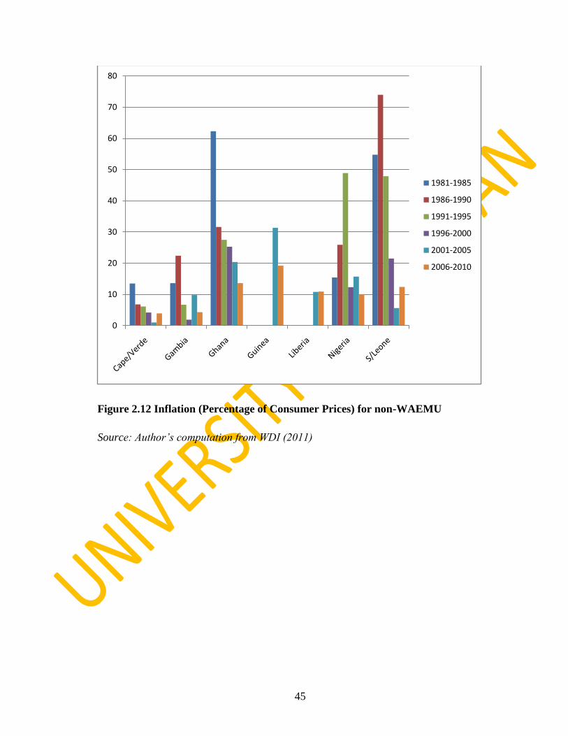
45
Figure 2.12 Inflation (Percentage of Consumer Prices) for non-WAEMU
Source: Author’s computation from WDI (2011)
0
10
20
30
40
50
60
70
80
1981-1985
1986-1990
1991-1995
1996-2000
2001-2005
2006-2010

46
Form figure 2.11 and 2.12, it can be seen that inflation is most prevalent among the non-
WAEMU countries. Inflation among the WAEMU countries has been low over the entire
period of the analysis. For these countries, inflation has been largely below 10% over the
entire period of this analysis. The only notable exception has been Guinea –Bissau where
inflation has been high; with the highest point being 57.5 within the period 1986-1990.
The country is a stand-alone among the WAEMU countries due to the fact that it was not
a French colony before but Portuguese and its currency was not pegged within the CFA
ambit until 1997 when it decided to join the CFA zone. Among the non-WAEMU
countries, Cape Verde and Gambia have maintained a relatively low inflation rate
compare to the other countries in the group. Nigeria, Sierra Leone and Ghana are the
countries with the higher prevalence with Sierra Leone being the highest.
2.3 Lesson for Macroeconomic Stability
In the West African region, the WAEMU sub-region has demonstrated more
determination and effort towards integration into the global economy. As noted earlier, the
integration within WAEMU has a multilateral surveillance mechanism whose ultimate
goal is to ensure the convergence of member economies. Convergence can generally be
achieved through two distinct patterns: nominal convergence, which focuses on the
evolution of nominal variables, and real convergence which requires the approximation of
living standards. WAEMU countries, adopting an approach similar to that of the European
Union, have opted for a convergence of nominal variables and assuming that nominal
convergence will lead to real convergence. In addition, theorists of optimum currency
areas argue that in a monetary union, the focus should instead be put on real convergence
that will eventually lead to nominal convergence. Furthermore, looking for a nominal
convergence can be very costly, especially for the poorest countries that are often remote
from nominal objectives adopted, and could even lead to real divergence raising behavior
of "free Ridding" in response to asymmetric shocks. To avoid this, WAEMU countries
found it necessary to adopt a Pact of Convergence, Stability, Growth and Solidarity. The
implementation of this pact is supposed to stabilize the economic situation and the
macroeconomic policies of the Union to ensure the harmonious development of member
countries.

47
As can be observed from figure 13, the change in reserves in the non-WAEMU region is
greater suggesting greater instability and the frequency of resorting to reserves for
stabilization. This is also observed in the inflation rate figure and the other
macroeconomic variables/indicators discussed above. Therefore, it can be concluded that
the WAEMU zone is faring better than the non-WAEMU zone in terms of macroeconomic
stability and performance convergence. This is mainly due to the fact that the WAEMU
members have been together as a union since after the colonial era. They were established
by France and survived after independence. This was not the case with the non-WAEMU
members. In the case of the latter, the WACB gave way to individual central banks soon
after the colonial era. The countries in the Anglophone area disintegrated and stood
independently without recourse to the WACB after each of their respective political
independence. Nevertheless, the issue of a common currency contemplation,
complimented by a common history and culture under the British colonial era is fostering
the economic and monetary integration processes in the non-WAEMU.

48
Figure 2.13. Change in Reserves for WAEMU and non-WAEMU (1982-2012)
Source: Author’s computation from WDI (2011)
-8000
-6000
-4000
-2000
0
2000
4000
6000
8000
10000
12000
WAEMU Change in Reserves Non-WAEMU Change in Reserves

49
2.4 Lessons from the Euro Zone Crisis for Macroeconomic Stability
Monetary cooperation among the European countries started with the establishment of the
European Monetary Society (EMS) in March 1979 with the aim of gaining closer
monetary cooperation which was supposed to result in monetary stability among the
member nations. There were three major stages in the integration process. The first stage
commenced in 1990 with the goal of strengthening both monetary and non-monetary
cooperation within the existing framework. The second stage commenced in 1994 with
twin aims of the preparation for the establishment of the European Central Bank (ECB)
and the achievement of economic convergence. The third stage was the launch of the
monetary union. The EMS became the EMU at the beginning of 1999 with the
introduction of the Euro and a common monetary policy by the ECB.
The crisis started due to the fact that the Euro zone is characterized by countries with both
strong and weak fundamentals. Some of the countries in the zone long suffered from
domestic instability that prevented them from meeting the pre-requisites for entry into the
EU. Belgium had a huge amount of debt that was over 100% of GDP; Italy had a history
of political instability and frequent change of government which led to the accumulation
of large fiscal deficits that weakened their local currency; Greece, Spain and Portugal
(also known as the peripheral countries) have long history of dictatorship which ended in
1974, 1975 and 1976 respectively which left them with fiscal, currency and monetary
problems (Okafor, 2010; Nindi, 2011).
The currency union did not result in deeper economic integration as initially envisaged
due to harmonization issues between the core countries and the peripheral countries. This
resulted in an unbalanced Euro zone with its members having divergent fiscal and
economic policies and wildly differing economic growth rates. Greece Italy, Spain and
Portugal misrepresented their economic performance to give the impression of their
readiness for union. This meant that these countries entered the EU when they were not
ready for monetary union. As the tide of the global economic crisis became stronger, the
lack of macroeconomic stability in these countries subsequently led to the sovereign debt

50
crisis as their economies could not withstand and sustain the strict monetary and exchange
rate policy of the EMU.
The discussion on the root causes of the EU crisis raised some important lessons for
macroeconomic stability if the prospect of a reserve pool in ECOWAS will be a success.
Given that there are countries with strong and others with weak macroeconomic
fundamentals in the region just as it was with the EU, it is crucial that measures must be
taken to bring about relative harmony within the region as polarised development between
the core and peripheral countries in the EU turned out to destabilised the EU. Moreover,
the success of a pool will require an ex ante harmonization of monetary policies of
member states and accurate growth rate preconditions while any form of misrepresentation
as it was with Greece, Italy, Spain and Portugal will adversely jeopardized the success of
the pool.

51
CHAPTER THREE
LITERATURE REVIEW
3.1. Review of Theoretical Literature
In this subsection, three main theories are reviewed. They arethe theory of demand for
reserves otherwise known as the buffer stock model,the optimum currency area and the
theory of club. These theories cover a large spectrum of framework that are of interest to
this study. The theory of demand for reserves is central to the examination of the
determinants of international reserves; the theory of club goods is on issues of reserves
pooling and optimum currency theory forms the basis for the analysis of issues central to
macroeconomic stability. These theories are discussed extensively in the following sub-
sections:
3.1.1. Theory of Demand for Reserves: The Buffer Stock Theory
Traditional theory describes external reserves holding as a function of variations in the
balance of payments, the opportunity cost of holding reserves, the scale of the economy,
trade openness, etc. Heller, 1966; Frenkel and Jovanovic, 1981; Lane and Burke, 2001;
Flood and Marion, 2002; Frenkel, 1978; Ben-Bassat and Gottlieb, 1992). The main reason
why countries hold foreign exchange reserves is to smoothen unpredictable and temporary
imbalances in international payments. Traditional views in the literature on external
reserves emphasize the role of three main variables: (i) the benefit of building up reserves
stocks which is calculated by the reciprocal of the marginal propensity to import; (ii) the
opportunity cost of hoarding reserves which is the spread between interest rate earned by
reserves and the alternative social use of these resources; and (iii) the volatility of balance
of payments, to take into consideration the degree of synchrony between external flows.
According to Frenkel and Jovanovic (1981), optimal level of international reserves for a
country depends on the variability of international transactions. This dependence stems
from the notion that reserves serve as a buffer stock with role of

52
accommodatingfluctuations and adjustments in external transactions. The basic
assumptions of the theory are that the optimal stock of reserves depends positively on the
extent of these fluctuations (adjustments); and that the optimal stock of reserves depends
negatively on the market rate of interest so that the extent that international reserves earn a
return that is lower than the market rate of interest, reserve holdings entail forgone
earnings on reserve holdings. Thus, the optimal stock of reserves is determined by
considering two components of cost: (i) the cost of adjustment which is incurred once
reserves reach an undesirable lower bound, and (ii) forgone earnings. In view of these, the
monetary authorities choose the stock of reserves which balances the potential
macroeconomic adjustment costs incurred in the absence of reserves with the opportunity
cost of international reserves holding.16
The cost of adjustment, which is assumed to depend on the frequency of adjustment and
on the fixed cost per adjustment, stems from the need to reduce expenditures relative to
income so as to yield the desired balance of payments surplus that is necessary for the
accumulation of reserves. The exact mechanism through which real expenditures are
reduced and the adjustment is effected depends on the circumstances. It may take the form
of a decline in real income due to a deterioration of the terms of trade, or it may take the
form of a decline in the real value of nominal assets due to a rise in the price level that
accompanies the deterioration in the terms of trade or that may be the result of a
devaluation (in which case the cost might include the perceived political cost that is
frequently associated with having a depreciating currency).17
The optimal stock of
reserves yields the optimal combination of being able to finance a deficit by drawing on
reserves and of having to adjust in the face of a deficit by reducing expenditures relative to
income. Since, due to the postulated stochastic process, reserve holdings are random, we
16
That is, a country chooses a level of reserves to balance the macroeconomic adjustment costs
incurred if reserves are exhausted (the precautionary motive) with the opportunity cost of holding
them (IMF, 2003).
17
These two components of cost are interrelated: a higher stock of reserves reduces the probability
of having to adjust and thereby reduces the expected cost of adjustment, but this additional
security is acquired at the cost of higher forgone earnings.

53
assume the optimal stock is obtained by minimising the sum of the expected value of both
components of cost
In the original version of the theory by Heller (1966), the central bank chooses a level of
external reserves to balance the macroeconomic adjustment costs incurred in the absence
of reserves with the opportunity cost of holding reserves so that the total cost of
adjustment is therefore given by:
TCa = ΔB/M (1)
Where TCa is the total cost of adjustment, ΔB is the amount of external imbalance and M,
the propensity to import. The avoidance of these adjustment costs would be beneficial to
the country involved and it is very possible to avoid the adjustment to an external
disequilibrium if the monetary authorities of the country have resources at its disposal
which can be used to finance the external disequilibrium thus rendering the adjustment
unnecessary. The resources which are at the disposal of the monetary authorities and
which can be used for such contingencies are the liquid international reserves.18
These
reserve assets could have been invested productively. The differential between the social
yield on capital invested and the yield on liquid international reserves is the appropriate
concept of the opportunity cost of holding liquid international reserves. Thus, neglecting
the effects of portfolio composition, the opportunity cost of holding a given amount of
liquid international reserves is a function of its volume, and is given by:
TCf = r.R (2)
Where TCf is the opportunity cost of holding the liquid international reserves, r the
differential between the social rate of return on capital and the return (if any) on the
reserves and R the volume of liquid international reserves held.
The government of every country has the responsibility as well as the incentive to
maximise the welfare of its residents.In the expected effort by the government (monetary
authorities) to shift the community indifference curve to a higher level because they are
rational, the costs of adjusting to an imbalance in the international accounts and the costs
18
Liquid international reserves held by the monetary authorities are part of the total capital resources of a
country.

54
of financing have to be compared to each other. Ultimately, the least expensive way of
handling an international disequilibrium would be chosen.
In order to determine an optimal level of international reserves, which the monetary
authorities may wish to hold for precautionary motives, three important parameters are
investigated: the cost of adjusting to an external imbalance; the cost of holding liquid
international reserves; and the probability that there will actually be a need for reserves of
a given magnitude. The marginal cost of adjusting national expenditure (MCa) such that
the external imbalance is eliminated is given by
MCa= 1/M (3)
which is the first derivative of equation (1), and which gives the total loss of income due
to an adjustment to a given imbalance. The total cost of holding a given amount of
international reserves is given by equation (2), and the marginal cost of holding one
additional dollar of reserves (MCf) is therefore the first derivative of equation (2):
MCf= r (4)
The optimal level of international reserves is given by the amount which minimises the
total cost of adjusting and/or financing an external imbalance. At this point, the marginal
cost of adjusting has to be equal to the marginal cost of financing.19
The probability that
adjustment will have to be used as a means of providing for external balance is defined by
π. So that
MCf = r = π .1/M = MCa (5)
With both r and m parameters known, π can thus be calculated:
π = r . M (6)
Frenkel and Jovanovic (1981) hypothesise that reserves movements between the
occasional restockings are generated by an exogenous „Wiener process‟. This is a process
where the incremental change in reserves in a small time interval is distributed normally.
Frenkel and Jovanovic(op.cit) also assumed that the deterministic part of the incremental
19
Yet, while the cost of holding additional reserves is incurred with certainty, the cost of adjusting is
incurred only in the case that a cumulative balance-of-payments deficit of a certain magnitude actually
occurs.
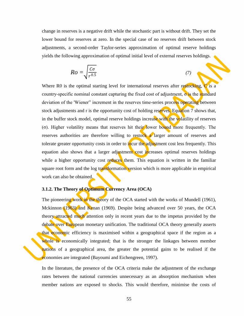
55
change in reserves is a negative drift while the stochastic part is without drift. They set the
lower bound for reserves at zero. In the special case of no reserves drift between stock
adjustments, a second-order Taylor-series approximation of optimal reserve holdings
yields the following approximation of optimal initial level of external reserves holdings.
Ro = 𝐶𝜎
𝑟0.5 (7)
Where R0 is the optimal starting level for international reserves after restocking, C is a
country-specific nominal constant capturing the fixed cost of adjustment, σ is the standard
deviation of the 'Wiener‟ increment in the reserves time-series process operating between
stock adjustments and r is the opportunity cost of holding reserves. Equation 7 shows that,
in the buffer stock model, optimal reserve holdings increase with the volatility of reserves
(σ). Higher volatility means that reserves hit their lower bound more frequently. The
reserves authorities are therefore willing to restock a larger amount of reserves and
tolerate greater opportunity costs in order to incur the adjustment cost less frequently. This
equation also shows that a larger adjustment cost increases optimal reserves holdings
while a higher opportunity cost reduces them. This equation is written in the familiar
square root form and the log transformation version which is more applicable in empirical
work can also be obtained.
3.1.2. The Theory of Optimum Currency Area (OCA)
The pioneering work in the theory of the OCA started with the works of Mundell (1961),
Mckinnon (1963) and Kenan (1969). Despite being advanced over 50 years, the OCA
theory attracted much attention only in recent years due to the impetus provided by the
debate over European monetary unification. The traditional OCA theory generally asserts
that economic efficiency is maximised within a geographical space if the region as a
whole is economically integrated; that is the stronger the linkages between member
nations of a geographical area, the greater the potential gains to be realised if the
economies are integrated (Bayoumi and Eichengreen, 1997).
In the literature, the presence of the OCA criteria make the adjustment of the exchange
rates between the national currencies unnecessary as an absorption mechanism when
member nations are exposed to shocks. This would therefore, minimise the costs of
56
joining an OCA (Araujo and Leon, 2004). Accordingly, the literature on the OCA theory
came to light in the early 1960s: a period characterised inter alia by the Bretton Woods
fixed exchange rate regime, capital controls in many countries and the incipient process of
European integration. Various OCA properties or criteria emerged; the OCA criteria are
reviewed next.
i. A High Degree of Factor Mobility
According to the OCA literature, one of the basic characteristics of an OCA is the
maintenance of a permanently fixed exchange rate between member nations. Mundell
(1961) therefore, suggests that the costs of an OCA are minimised when factors of
production (especially labour) can move freely within the area. The argument is that if
productivity or other shocks affect one nation/ region, resulting in a decline in its output
and real wages, factors of production may migrate to places of excess demand within the
currency area. The movement of factors of production avoids the need to adopt distinct
monetary policies by individual countries when shocks affect member countries
differently. High factor market integration within a group of partner countries can reduce
the need to alter real factor prices and the nominal exchange rate between countries in
response to disturbances. Trade theory has long established that the mobility of factors of
production enhances both efficiency and welfare. Such mobility is likely to be modest in
the very short run and could display its effect over time.
ii. A High Degree of Trade Openness
Changes in exchange rate are often transmitted to the price of tradables and hence the
domestic economy. As such, consumers tend to be wary of any changes in the exchange
rate and thus, there is little money/exchange rate illusion by wage earners. The result of
this is that nominal wages and prices tend to react quickly to the devaluation of the
currency thus making it less effective (McKinnon, 1963). The advantages of fixed
exchange rates will increase with economic openness, while those of flexible rates decline.
It is therefore noted that a high degree of trade openness prior to forming an OCA
increases the benefits and reduces the costs of doing away with the exchange rate as an
adjustment tool. Also, a devaluation would be more rapidly transmitted to the price of
tradables and the cost of living, negating its intended effects. Hence the nominal exchange

57
rate would be less useful as an adjustment instrument. Economic openness needs to be
assessed along several dimensions, including the overall openness of a country to trade
with the world; the degree of openness vis-à-vis the countries with which it intends to
share a single currency; the share of tradable versus non-tradable goods and services in
production and consumption; and the marginal propensity to import. These dimensions of
openness overlap but are not synonymous. The literature has shown that monetary
integration catalyses openness further that is, the “endogeneityof OCA”. (Frenkel and
Rose, 1998; McKinnon, 1963).
iii. A High Decree of Product Diversification
Product diversification ensures that an economy has a degree of insulation against a
variety of shocks. High diversification in production and consumption, such as the
“portfolio of jobs”, and correspondingly in imports and exports, dilutes the possible
impact of shocks specific to any particular sector. Therefore, diversification reduces the
need for changes in terms of trade via the nominal exchange rate and provides “insulation”
against a variety. Nations ought to have highly diversified economies prior to forming an
OCA (Kenan, 1969; Nindi 2011). If a nation that produces a variety of goods is hit by a
shock, the subsequent changes in the prices of the goods would also vary differently.
Hence, if the shock is specific to a good or industry, there is a possibility that the economy
as a whole will not be adversely affected as that particular good or industry (Araujo and
Leon, 2004). Vaubel (1978) and Bayoumi and Ostry (1997) note similarly that if trade
between members of an OCA is highly diversified, the law of large numbers implies that
the probability and the size of changes in each country's terms of trade is reduced when hit
by an economic shocks.
iv. Price and Wage Flexibility
When nominal prices and wages are flexible between and within countries contemplating
a single currency, the transition towards adjustment following a shock is less likely to be
associated with sustained unemployment in one country and/or inflation in another. This
will in turn diminish the need for nominal exchange rate adjustments (Friedman, 1953).
Alternatively, if nominal prices and wages are downward rigid some measure of real
flexibility could be achieved by means of exchange rate adjustments. In this case the loss

58
of direct control over the nominal exchange rate instrument represents a cost (Mongeli,
2010).
v. Financial Market Integration
Ingram (1973) noted that financial integration can reduce the need for exchange rate
adjustments. It may cushion temporary adverse disturbances through capital inflows – e.g.
by borrowing from surplus areas or decumulating net foreign assets that can be reverted
when the shock is over. With a high degree of financial integration even modest changes
in interest rates would elicit equilibrating capital movements across partner countries. This
would reduce differences in long-term interest rates, easing the financing of external
imbalances but also fostering an efficient allocation of resources. Financial integration is
not a substitute for a permanent adjustment when necessary: in this case, it can only
smoothen this process. Temporary financial flows may induce a postponement of real
adjustment and render it more difficult at a later stage. Some authors also warn that
financial integration might lead to destabilising capital movements (Mongeli, 2008).
3.1.2.1 The OCAAsymmetric Shocks and Macroeconomic Stability Determinants
The OCA theory (Mundel, 1961; McKinnon, 1963; Kenan, 1969; Mongeli, 2002; Debrun,
Masson and Patillo, 2005; Ricci, 2008) identifies the sources of asymmetric shocks to an
economy to cover a wide spectrum in the literature. These include exchange rate
variability, output variation, variation in terms of trade and trade flow and variation in
consumer price index. Also, in the literature, asymmetric shocks are traced to fiscal policy
distortions resulting from public expenditure, deficit financing and investment. High
inflation, volatile export revenues, or variable economic growth addto the risks faced by
agents and thereby worsen the prospects of economicactivities that pay off in the future.
These uncertain environments aretherefore detrimental to investment, skills learning, and
in general he development of businesses. Empirical studies have indeed found a
significant statistical relationship between inflation and growth, even after controlling for
fiscal performance, wars, droughts, population growth,openness, human and physical
capital and after allowing for simultaneitybias. Output variability and exports or terms-of-
trade volatility are the othercommonly used measures of macroeconomic stability.

59
According to Satyanath and Subramanian(2004),there are a number of different ways in
which macroeconomic instability can be the consequence of distributionally-motivated
actions by governments or others in power.First, in early (Marxian) analysis of business
cycles, the expansion of bank credit during booms was seen as providing extra purchasing
power for business to finance investments beyond that would have been possible without
inflation. This inflationary financing of an investment boom is made possible by implicitly
depressing private consumption (consequent upon the real wage decline that accompanies
inflation) and thereby increasing savings. Second, inflation is an instrument par excellence
for redistributing wealth: for example, from creditors to debtors and away from those that
hold money and other assets (unskilled human capital) that cannot be hedged against
inflation.20
Third, while Marxian analysis of inflation tend to stress the conflict between wage-earners
and capitalists, in many developing countries, particularly in Latin America and Africa,
the fissures run as much between sectors as classes. The cleavage is often between urban
wage earners employed in nontradables and those that derive income from resource-
intensive export sectors.Any loosening of monetary and fiscal policies has inevitable and
intended redistributional effects. Often fiscal expansion takes the form of wage increases
granted to public sector employees in the urban sector. The rise in urban real wages
consequent upon these policies squeezes profits in the primary sector. Macroeconomic
expansion thus has distributional intent and consequences. Occasionally, inflation through
selective credit expansion serves to favour some industries over others (in Brazil in the
mid-1960s, this was deployed to favour the automobile sector at the expense of basic and
consumer goods).
A fourth case relates to borrowing and rising government indebtedness, which often
substitutes for inflation as a means of financing unsustainable spending plans and hence
promoting the interests of a particular group in society. Much of the reason for high
inflation and external instability results from the vast overhang of external debt. The
reasons for this debt accumulation are complex, but include both domestic factors
20
For example, in Chile in the 1870s, land owners were accused of orchestrating inflation to permit
them to repay their loans in depreciated paper money.

60
(including populist policies). Thus, borrowing and indebtedness are simply another
manifestation of nominal instability and hence related to the same underlying causes.
Finally, another adverse impact of polarisation within society on macroeconomic
stabilisation has been analysed. If countries need to pursue costly stabilization in the wake
of shocks and different interest groups disagree on the allocation of the burden of
adjustment, a struggle ensues between them, with each trying to make other groups pay
for the adjustment. Successful stabilisations are then delayed until one group consolidates
its position and prevents the others from vetoing the stabilisation plan. Thus, latent
conflict in society leads to greater macroeconomic instability.
The sources of shocks identified by the OCA are critical to this study as they form the
bases for the macroeconomic variables employed. Debrun et al (2005) and Ogunkola and
Jerome, (2005) stressed that the region face shocks asymmetrically due to the differences
in their terms of trade and most especially the differing content of their respective exports.
3.1.3 The Theory of Clubs
James M. Buchanan developed club theory21
in his 1965 paper, "An Economic Theory of
Clubs"22
. He wrote that there was an "awesome Samuelson gap between the purely private
and purely public good". This gap contained goods that were excludable but shared by
more people than typically share a private good but less people than typically share a
public good. The goal of his theory was to address the question of determining the "size of
the most desirable cost and consumption sharing arrangement". An example of private
goods that Buchanan offered to illustrate this concept was the used of a pair of shoes by a
group of people. Two people cannot wear the same exact pair of shoes at the same time.
However, two or more people can take turns wearing them. As the number of people
sharing the same pair of shoes increases the amount of utility each person derives from the
shoes diminishes. As more persons are allowed to share in the enjoyment of the facility of
a given size, the benefit evaluation that the individual places on the good will, after some
point, decline. There may, of course, be both an increasing and a constant range of the
total benefit function, but at some point congestion will set in, and their evaluation of the
21
The study of club goods in economics 22
There were latter modifications by Dodsworth (1975) and Ng (1975).

61
good falls. But each new member or co-owner helps reduce the cost of the club good so
there will be some optimal size of the good that maximizes the benefit for its members.
Assumptions of the Theory of Clubs
i. Differing Utilisation Pattern (Asymmetric Utilisation)
The demand and utilisation pattern of the club‟s resources by members should not be
similar. This assumption is necessary to avoid crowding and congestion in the use of the
resources. Club goods have artificial scarcity. By this, it means that congestion can reduce
access to the resources by the members when demands are made at the same time as
congestion takes the form of a non-excludable public “bad” within the club. This is one
assumption that distinguishes a club good from a pure public good which is considered to
be fully non-rivalrous. The non-rivalrous23
property in public economics holds when the
use of a unit of the good by one consumer does not preclude or diminish the benefit from
another consumer using the same unit of the good. Thus, there is jointness in consumption
of the good - one unit of the good produced generates multiple units of consumption.
Rivalrousness is a more continuous concept. The degree of rivalrousness can be defined
by the size of the marginal opportunity cost of an additional user attempting to use the
resources at the same time two or more other members are using it. Zero is one extreme.
Therefore, as much as possible, the members of a club must differ their utilisation of the
resources of the pool as to even out over crowding at a particular point in time.
ii. Finite and Optimal Size
In the theory of clubs, it is assumed that the size of the members is finite. The dynamics of
the situation would suggest that a small membership size is optimal. This is to suggest that
there has to be a limited degree of publicness as additional members beyond the optimal
membership size will impose a cost on existing members. As with the case of the reserves
pool, congestion may arise due to “infinite membership” thereby reducing the marginal
utility of existing members. According to Ng (1975) the relevant Pareto optimality
23
Non-rivalrous implies that the opportunity cost of the marginal user is zero just as in the case
where one consumer‟s listening to a broadcast does not diminish another‟s ability to benefit from
the same broadcast

62
condition requires that any individual in the club must derive a total benefit in excess of
the aggregate marginal cost imposed on all other consumers in the club. So the Buchanan-
Ng theory is to optimise the membership while considering the degree of congestion or
overcrowding to be equally important.24
However Buchanan (1965) opines that a club
should admit more members so as to maximise the difference between total benefits per
person and total costs per person due to the club.25
The club facilities should be increased
until the added marginal benefit per person is equal to the additional total cost of making
the facility bigger.
iii. Non-excludability and Unrestricted Access
It is assumed that members of the club have unrestricted access to the common resources
of the club. However, other members of the general public are excluded from accessing
the resources of the pool. In the case of a reserves pool, each member has unconstrained
access to the pool. Since the pool belongs to all members, it is believed assumed that
whenever in need in terms of a financial constraint or macroeconomic instability in the
country, the member can so resort to drawing from the pool. Resources from a club are
sort of public goods that are non-rivalrous, at least until reaching a point where congestion
occurs among members.
In common property regimes, access to the resource is free to members however,
common-pool resources are not public goods. While there is relatively free but monitored
access to the resource system for community members, there are mechanisms in place
which allow the community to exclude outsiders from using its resource. Thus, in a
common property regime, a common-pool resource appears as a private good to an
outsider and as a common good to an insider of the community. The resource units
withdrawn from the system are typically owned individually by the appropriators. A
common property good is rivaled in consumption.
iv. Non-discrimination
Here it is assumed that costs and benefits from the operation of the club are shared equally
24
Club theory has many interesting applications in the analysis of congestion and in establishing
the optimal group size for (say) a local golf club to a local community. 25
That is, the club should admit more members so long as the reduction in costs per person is
greater than the reduction in benefits per person due to increased costs of congestion.

63
among the members of the club. It is assumed that there is no discrimination in the
distribution of gains. Further, the theory of clubs assumes that the cost of reduction of
additional entry is split equally among the club members and that the added loss in benefit
resulting from additional entry is also evenly shared. That is, no one needs to pay a
disproportionately large fraction of the costs, and different people do not have different
levels of sensitivity to crowding. Coase (1960) proposes a mechanism by which
beneficiaries of a public good band together and pool their resources based on their
willingness to pay to create the public good. If the transaction costs between potential
beneficiaries of a public good are sufficiently low, and it is therefore easy for beneficiaries
to find each other and pool their money based on the public good's value to themselves,
then an adequate level of public goods production can occur even under competitive free
market conditions.
v. Non-profligacy
This assumption attempts to place restriction on the extravagance that can arise from the
wasteful behaviour of some members of the club. Even though the use of resources of a
club is seen to be non-rivalrous this can only be up to a point. This assumption is
synonymous with the issue of free-riding in the provision of public goods. As with public
goods, club goods also provide a very important example of market failure, in which
market-like behaviour of individual gain-seeking does not produce efficient results. If
private organisations do not reap all the benefits of a public good which they have
produced, their incentives to produce it voluntarily might be insufficient. Consumers can
take advantage of public goods without contributing sufficiently to their creation. This is
called the free rider problem because consumers' contributions (marginal cost) will be far
less than the marginal benefit they are getting from the club. If too many members decide
to “free-ride”, private costs will exceed private benefits and the incentive to provide the
good or service disappears. The club (market) thus fails to provide a good or service for
which there is a need. The free rider problem depends on a conception of the human being
as homo-economicus: purely rational and also purely selfish-extremely individualistic,
considering only those benefits and costs that directly affect him or her. Public goods give
such a person an incentive to be a free rider. Therefore, if some people crowd more than
others, they can be charged more to compensate for the reduction of the benefits they

64
bring about. If club owners are allowed to price-discriminate, they will not need to
categorically exclude anyone from joining.
vi. Common Arbitrator
In the theory of clubs, it is assumed that there is a common regulator/arbitrator who
monitors and controls the use of the resources of the pool. The regulator is responsible for
the preservation, maintenance, and consumption of the common-pool resource.The need
for an arbiter arises so that members cannot act independently to threaten the total net
benefit from the common-pool resource. So in order to maintain the resource system,
these arbiters coordinate their strategies to keep the resource as a common property,
instead of dividing it up into bits of private property. They typically protect the core
resource and allocate the fringe through complex community norms of consensus
decision-making. Common resource management has to face the difficult task of devising
rules that limit the amount, timing, and technology used to withdraw various resource
units from the resource system. Setting the limits too high would lead to overuse and
eventually to the destruction of the core resource, while setting the limits too low would
unnecessarily reduce the benefits obtained by the users.
The theory provides the basis for which reserves pooling decisions can be related to the
institutional and structural characteristics of a given federation. The main idea in the
theory of clubs is that if the utilization patterns of members of a club are not highly
positively correlated, then the members could be better off by sharing each others‟
facilities so as to even out crowding. The club is assumed to still be in the planning stage
and membership as well as the cost sharing scheme are still the subject of bargaining. The
setting here is a group of countries (or regions) formed in a federation which facilitates
some type or group decision-making. Each country in this group is supposedly part of an
optimal club with a central authority.
The subject of the club theory is a common-pool resourcesalso called a common property
resource. It is a type of good consisting of a natural or human-made resource whose size
or characteristics make it costly, but not impossible, to exclude potential beneficiaries
from obtaining benefits from its use. Unlike pure public goods, common pool resources
face problems of congestion or overuse, because they are subtractable. A common-pool

65
resource typically consists of a core resourcewhich defines the stock variable, while
providing a limited quantity of extractable fringe units, which defines the flow variable.
While the core resource is to be protected or nurtured in order to allow for its continuous
exploitation, the fringe units can be harvested or consumed. Because their core resources
are vulnerable, common-pool resources are generally subject to the problems of
congestion, overuse, pollution, and potential destruction unless harvesting or use limits are
devised and enforced.
The use of many common-pool resources, if managed carefully, can be extended because
the resource system forms a positive feedback loop, where the stock variable continually
regenerates the fringe variable as long as the stock variable is not compromised, providing
an optimum amount of consumption. However, consumption exceeding the fringe value
reduces the stock variable, which in turn decreases the flow variable. If the stock variable
is allowed to regenerate then the fringe and flow variables may also recover to initial
levels, but in many cases the loss is irreparable.
According to Dodsworth (1975), the institutional problem for the central authorities of the
federation is to devise a cost sharing scheme which would attract unanimous support from
members of the group. Each country in the federation is faced in a time period, t, with
financing a level of payments, Dt. This it does from current receipts, Ct, which are geared
towards an average or forecast expenditure. The expenditure, (if it is greater than current
receipt) is financed from a contingency reserves fund, R. The size of this reserves fund
will depend primarily on some measure of dispersion of Dt above Ct, and on a risk factor:
(8)
In this formulation receipts and outgoings are taken as given and remained unchanged
whether the country is in or out of the club. While for the three remaining variables, R, w
and n, the choice of any two determines the third, or, alternatively, the choice of one, say,
R, determines a set of combinations of w and n. The number of time periods involved will
depend on the type of fund being considered. If recourse can be made easily to higher
governmental units, then n may be quite small. However, if the untypical case of
1 1
( )n n
t t
t t
w pr D C R
66
international reserves where confidence is all important is taken, n would generally be
expected to be very large and w, correspondingly, very small. The determination of the
common risk factor is of interest here as choice must be made between the public and
private benefits of the club.
According to Medhora (1992), under an international reserves pooling arrangement, a
common central bank must be in operation; one of whose main responsibilities is to
oversee the external operations of the member countries so that the existence of a common
pool of official international reserves provides a service with potential benefits for some or
all of the members. A crucial requirement for the success of any pooling scheme is one of
non-profligate behaviour on the part of all its members. If one or more member(s) change
their pattern of reserves use after pooling, then (a) any ex ante gains will not be realized as
forecast, and therefore, (b) the pooling arrangement might break down. More specifically,
if one member inflates inappropriately after pooling, and thus draws down the common
reserves knowing that it now has access to more reserves than before, then the other
members might be tempted to do the same, or opt out of the pool. Thus, the presence of a
controlling central bank can checkmate such profligate member. And a single country
cannot continuously draw down the pool without evoking a warning signal from the
central monetary authority or response from the other member countries.
In the case of the WAEMU zone, each country maintains a separate account with the
common central bank called the BCEAO. In the first instance, each country draws down
its own account of pooled and unpooled reserves. If these are fully drawn down, the other
countries' pooled reserves may be used. The French Central Bank oversees the operation
of the BCEAO and it augments the Operations Account only when all the Union‟s
reserves have been fully drawn down. Also, no limit is placed statutorily on a member
country‟s use of the entire pool. A crisis management scheme is immediately employed by
the central bank only when the entire pool falls below a particular threshold (Medhora
1992).
As stated earlier, the club model provides a framework in which gains from a possible
reserves pooling can be assessed. The assumptions here are as discussed earlier to include
differing utilisation pattern, non-excludability and unrestricted access, non-discrimination

67
among members, non-profligacy, common arbitrator and finite and optimal size of the
club.In an early application of the theory of clubs to reserve pooling, Dodsworth (1975)
describes the gains this way:
“so long as the risk of abnormal demands on the reserve position is
proportionately less when spread over a number of countries, then
reserve economies are possible. Either total reserves required can be
reduced or individual countries can benefit from an increased level of
insurance cover.”
This is the fundamental pillar on which gains from pooling can be assessed. The potential
gains from pooling reserves arise from the lower risk that results when reserves that show
different patterns of use are combined among a group of countries. Similar gains arise
from a range of pooling schemes whether it is unemployment insurance funds, health
plans, or mineral reserves. By belonging to a reserve pool, the member countries have
unconditional access to the others' reserves during times of need. At the same time, by
pooling, each country is accountable for and “taken upon itself” the variability of the
entire pool, rather than just the variability of its own reserves. Starting with the
proposition that variability, as a proxy for risk, is undesirable, then a scheme that
potentially reduces variability and increases access to reserves offers greater protection for
the same level of risk, or alternately, requires fewer resources for the same level of
protection as before; this is how the idea of “coverage” is born. In customary
policymakers' parlance and in the context of international reserves,the term coveragerefers
to the number of weeks/months of imports they can pay for. In the context of risk aversion
among holders of international reserves, it is more appropriate to consider coverage as the
ratio of reserve holdings to their variability.
According to this formulation, coverage will increase if there is an increase in access to
reserves or a decrease in reserves variability. Coverage incountryiis defined as
(9) ( )
ii
i
PRC
Var PR
68
Where PRiis the average level of reserves during a time period and VAR (PRi) is their
variabilityduring the same time period (for each country); and for reserves pool, PR =
. This formulation above encompasses two potential sources of gains in reserve
pooling:(i) access to increased reserves holdings; (ii) possible reduction in reserves
variability.In both cases, coverage will increase.Variability is represented by the
coefficient of variation of the reserve during a specified time period.
3.2 Benefits and Costs of Reserves Pooling
Belonging to a regional reserves pooling scheme can be beneficial. It is used in
emergencies and is expected to expand the capacity of the countries in the region in order
to tackle any financial crisis, as well as contribute substantially to the economic stability
of the region. With such a reserve pool in place, timely financial assistance can be offered
to any crisis-stricken economy in the pool and it will also prevent further collapse as well
as spread to other economies within the pool (Fafchamps et al, 2007).
According to Basu et al (2010), the existence of trade linkages among countries means
that self- insurance strategy by one country has externalities for other countries so that a
crisis in one country reduces the demand for goods produced by its trading partners, and
therefore is also costly for neighbouring countries. In the absence of reserve pooling,
countries use their savings to self-insure themselves first against external shocks, without
taking into account the effect of their actions on the welfare of their neighbours or trading
partners. However, regional reserves pooling arrangements can internalize this externality
and thereby increase welfare for all countries involved.
Countries can be subjected to two broad categories of shocks: financial and business cycle
shocks and the transmission of such shocks to other countries is possible in this
globalization era (Basu et al, 2010). For the purposes of a reserves pooling arrangement,
financial shocks are regarded as exogenous while business cycle shocks as an endogenous
outcome of the policies pursued by the reserves pool. This observation should inform how
intraregional and inter-regional shock correlations be measured. The higher the correlation
of financial/business cycle shocks within rather than across regions, the less attractive is a
regional pool. The stronger the terms of trade effects of shocks within a specific region,
the more attractive is such a pool (Cole and Obstfeld, 1991;Tesar, 1993; van Wincoop,
iPR

69
1999;Athanasoulis and van Wincoop, 2000).
There are other benefits associated with moving from self-insurance to a reserves pooling
arrangement within a region: the unification of budget constraints results in a single
borrowing limit for the reserves pool as a whole and this improves welfare by expanding
the set of feasible allocations. Furthermore, the pooling of reserves improves the
diversification of idiosyncratic country endowment risk. The benefits of diversification are
greater when the trade externality is internalised within a regional pool (Basu et al, 2010).
There are costs associated with a country participating in the pooling of reserves with
other members of the region. These costs include the following: first, the loss of
independent monetary policy; in this regard, it can be recalled that it was earlier stated that
external reserves are often deployed when the market clearing exchange rate undershoots
or overshoots the level that is consistent with the attainment of the prime goal of
macroeconomic stability. Reserves are often used for the defense of the value of the local
currency. This is supposed to suggest that foreign reserves are potent tools in the hands of
the monetary authorities of any economy. Thus, if a country does not have access to its
reserves, having ceded same to the union, then the country becomes impotent and
dependent on the monetary policy coming from the central monetary authority of the
union at large. This fear of the loss of power to affect a national money supply is
legitimately a great one since in an integrated market, all member countries will jointly
control their monetary policy. Typically, the loss of a country‟s ability to use the exchange
rate and monetary policy for stabilization was considered to be the most important cost of
joining a currency area. However, this is surely not the case for small open economies,
because it is impossible to maintain free capital mobility and an independent monetary
policy together. Such countries link their currencies to their main trading partners in order
to gain higher exchange rate stability. This lowers the independence of monetary policy
(Horvath and Komarek, 2002).
Second, the economy loses seigniorage, which comes as a source of revenue to the
government. Seignorage is the revenue the government obtains by financing its budget
deficit through printing money rather than selling debt. That is why at full employment
printing money would lead to inflation. Seignorage is frequently also called the „inflation

70
tax‟. It is largely a policy question how seignorage would be distributed in the case of
monetary union.In Western Europe only in some southern countries seignorage was
estimated to be more than one percent of GDP and the ratio is rapidly decreasing in time
(Oyejide, 2012; Ricci, 2008; Abeng, 2007).
Third, asymmetric shocks; this cost encapsulates exchange rate variability, output
variability, terms of trade as well as variation in consumer price index. If the movements
of exchange rates reflect feelings, speculation etc., then high volatility could lead to
misallocation of resources. The cost of pooling increases significantly within a group on
countries in a region when they face these shocks asymmetrically.
Fourth, fiscal policy distortions; some centralization of fiscal policies could serve as one
of the mechanisms in adjusting to asymmetric shock, however, the centralization of
budgets often leads to an increase in spending. Also, a country belonging to a pool
becomes “responsible” for the management of the economy of other members. When a
member is faced with any macroeconomic perturbation beyond its control, other members
of the union are obliged to provide support and bail the ailing economy out so as to reduce
the risks of spread of the “ailment” to other members in the pool. Therefore, the pattern
and size of income/revenue as well as spending of (potential) members becomes an issue
of serious consideration (Masson and Pattilo, 2002).
3.3 Methodological Review
A major concern of this study is the assessment of gains for member countries of
ECOWAS if their international reserves are to be pooled together. A review of the
literature shows that the concept of coverage,which dovetails from the theory of club
goods, has commonly been deployed to explain and test for the presence gain/loss when a
group of countries are to pool reserves together. In the context of risk aversion among
international reserves holders, coverage is appropriate considered to be the extent to which
an economy can be shielded by its available foreign reserves from both domestic and
external macroeconomic perturbations. This methodology has been used in the studies by
Williams, Polius, and Hazel (2001) where a comparison of the gains from the pooling of
reserves, and hence reserve variability, in the Eastern Caribbean Currency Union (ECCU)

71
and the CFA franc zone was presented. This methodology is employed when Rajan,
Siregar and Bird (2003) examines the case of reserves pooling in East Asia. The study is
an investigation of the gains, if any, to be reaped if the East Asian economies were to pool
their reserves. In a related study, Rajan and Siregar (2004) applied the method of coverage
in their work on centralized reserve pooling for the ASEAN plus three (APT) countries.
Medhora (1992) investigates the case of reserves pooling in the CFA zone and the method
of coverage was applied. In a related study, Callen, Imbs and Mauro (2009) constructed a
list of country pools from a large sampleto study risk pooling. Here, the volatility of pool-
wide gross domestic product growth was computed and compared with the volatility in
each country individually. The viability of a single monetary zone in ECOWAS was
evaluated by Ogunkola (2005). An estimation of the costs and benefits of a monetary
union in the region was carried out using the real exchange rate (RER) variability model.
This methodology is used to show that West African countries are closer to forming a
single monetary union now than before.
Elhiaraka and Ndikumana (2007) have examined issues of reserves accumulation among
African countries using the methodology of panel cointegration and error correction
mechanism where they attempt is made to identify the sources, motivations and effects of
such reserves accumulation in Africa. Ruiz-Arranz and Zavadjil (2008) examine whether
foreign exchange reserves in emerging Asia have grown beyond what is needed to support
financial stability. They use a threshold model and assess the benefits of reserves in terms
of reduced borrowing spreads. They adopt the insurance model of optimal reserves as a
framework, based on the work of Jeanne (2007) which has it that reserves enable an
economy to cushion the impact of a sudden stop in capital flows on domestic consumption
and output by providing a ready source of liquidity. They estimate spreads-reserves
elasticities for a panel of 34 emerging economies for the period 1997–2006. By applying
this methodology, they endogenously determine the threshold level(s) of reserves and
confidence intervals at which the relationship between reserves and spreads changes
where they show that most of Asia can still benefit from higher reserves in terms of
reduced borrowing costs.

72
In the examination of the question of adequacy of reserves in sub-Saharan Africa (SSA) in
the light of the shocks faced by these countries, Drummond and Dhasmana (2008) extend
the Jeanne and Ranciere (2006) reserves model of consumption smoothing and applies it
to experiment reserve holdings in SSA in the light of likely shocks. The authors, in their
methodology, make use of simulation. The country simulations considered here take into
account various aspects of vulnerability. They consider a Small Open Economy (SOE)
model with two goods- one tradable and another non-tradable. The use of this model
allows for the simulation of the optimal level of reserves across a broad spectrum of
shocks and output costs, but this level is sensitive to the choice of key parameters such as
the risk aversion, the term premium and the probability of shocks, and results in the paper
are illustrative of model simulations for a given set of parameters.
The time consistency model framework is adopted by Lin and Wang (2005) to show how
the intervention of the monetary authority influences the domestic economy in five East
Asian economies: Japan and four Tigers (Hong Kong, Korea, Singapore and Taiwan).
They analyze the relationship between foreign exchange reserves and inflation rate
through the operations of the foreign exchange market. This study is an extension of the
time consistency model developed by Kydland and Prescott (1977) to incorporate
exchange rate stability in the policymaker's objectives. A regression model is set for the
empirical study where inflation rate is measured as the annual change in Consumer Price
Index (CPI) and estimated with a correction for serial correlation using Cochrane-Orcutt
method. In a related study, Gosselin and Parent (2005) conduct an analysis of foreign
exchange reserves in Emerging Asia. They attempt to measure how far the current level of
reserves is from that predictedby the standard macroeconomic determinants in Asia. They
adopted the buffer stock model as a framework and then usePedroni‟s (1999) panel
cointegration tests as the basis for the estimation of a long-run reserves demandfunction in
a panel of eight Asian emerging-market economies: China, India, Indonesia, Korea,
Malaysia, the Philippines, Singapore, and Thailand.
By way of summary of the methodological review undertaken, it is observed that the
coverage index has commonly been deployed to explain and test for the presence of
gain/loss in a reserves pooling scheme. As mentioned earlier, coverage is considered to be
the extent to which an economy can be shielded by its available foreign reserves from both

73
domestic and external macroeconomic perturbations. This methodology was employed in
the study by Williams, Polius, and Hazel (2001). Also, it is employed when Rajan, Siregar
and Bird (2003). The study is an investigation of the gains in a reserves pooling
arrangement in the East Asian. In a related study, Rajan and Siregar (2004) applied the
coverage index in their work on centralized reserve pooling for the ASEAN (Association
of South-East Asian Nations) Plus Three (APT) countries.Medhora (1992) investigates the
case of reserves pooling in the CFA zone and the method of coverage was applied.
For the estimation of macroeconomic shocks, the correlation shocks and the vector
autoregressive framework (VAR), and by extension the structural VAR (SVAR), are
prominent methodologies widely employed in the monetary integration literature. The
VAR approach places minimal restrictions on how shocks from variables affect the
economy. This methodology is widely thought to be informed by the standard technique in
measuring shocks as pioneered by Blanchard and Quah (1989).
The review shows wide application of this methodology: Vaubel (1978), Bayoumi and
Eichengreen (1992), Erkel-Rouse and Melitz (1995), Frankel and Rose (1998), WAMI,
2005, Ogunkola (2005), Ogunkola and Jerome (2005). Masson and Patillo (2001)
employed the correlation of shocks to examine whether the ECOWAS region and the
West African Monetary Zone can be seen as a candidate for an optimum currency area.
Ogunkola (2005) and Ogunkola and Jerome (2005) constructed the real exchange
variance, as a yardstick, to determine the degree of asymmetric shock in West Africa
where the VAR framework is employed to estimate the real exchange variability as a
measure of shock. In spite of its wide application, most econometrician and analysts have
put forward that the VAR framework assumes interrelationships and interdependence
among economic aggregates without perspicuous recourse to theory. Other methodologies
widely employed are the ordinary least squares and the instrumental variable techniques
(Nnanna et al, 2007; Debrun, Masson and Patillo, 2005; Elhiraika and Ndikumana, 2007).
74
3.4 Empirical Review
There are no ample empirical evidences on reserves pooling specifically. Therefore it is
necessary to state that most of the investigations in the literature focus on issues
surrounding monetary integration as a whole and not purely on reserves pooling.
However, few studies have examined reserves pooling for some of the regions of the
world.Williams, Polius, and Hazel (2001) present a comparison of the gains from the
pooling of reserves, and hence reserve variability, in the Eastern Caribbean Currency
Union (ECCU) and the CFA franc zone. The results show that countries from the two
regions benefit from external reserves pooling. It was shown that countries within the
ECCU area have achieved greater balance of payments protection than the CFA zone
countries from the pooling of reserves. Unanticipated changes in the terms of trade
lowered reserves in the CFA zone relative to the ECCU, which may reflect a greater
reliance on primary commodities in the CFA compared with services in the ECCU.
In the study examining the case of reserves pooling in East Asia, Rajan, Siregar and Bird
(2003) investigate the gains, if any, to be reaped if the East Asian economies were to pool
their reserves. The highest overall average for the coverage index with pooling is found to
be at a 10 percent commitment; it implies a significant gain from pooling. They estimate
the coverage index for every 1 percent from 0 to 10 percent and then from 10 to 20
percent to locate the level of pooling that will most benefit the East Asian economies as a
group. Results show that based on the highest overall average of coverage index, as a
group, the economies stand to benefit most by committing to a one percent pooling
arrangement. Rajan and Siregar (2004), in a separate study, finds that before the Asian
financial crisis, countries in the ASEAN (Association of South-East Asian Nations) plus
three (APT) nations are better-off if they are to commit themselves to a partial pooling
scheme than a complete pooling as 50% pool coverage indices are in general higher than
those for the 100% pooling. For the post-crisis period, the results for benefit of pooling are
less conclusive as the result reveals that the advantages from reserves pooling are not self-
evident. The decline in the benefits of pooling after the crisis vis-a-vis before the crisis can
be largely explained by both significant increases in the average reserves levels as well as
the sharp declines in the variability of the reserves after the crisis relative to the pre-crisis.
75
Ogunkola (2005) evaluates the viability of a single monetary zone in ECOWAS and finds
that West African countries are closer to forming a single monetary union now than
before. An evaluation of the costs and benefits of a monetary union in the region shows
that there are significant potential benefits to be reaped in the form of significant savings
on foreign exchange as a result of reduced exchange rate risk, increased intraregional trade
as well as increased investments among others even though the benefits come at the cost
of loss of seigniorage and custom duties. Ogunkola and Jerome (2005) also support the
findings of possible gains. The results also show that the CFA zone has achieved greater
stability in general compared to its non-CFA counterpart in the ECOWAS subregion.
However, the results also reveal that the Structural Adjustment Programmes (SAP) in the
sub-region brought about stability in real exchange rate shocks to non-CFA ECOWAS
countries compared to its CFA counterparts.
A list of country pools from a large sample was constructed by Callen, Imbs and Mauro
(2009) to study risk pooling where the volatility of pool-wide gross domestic product
growth was computed and compared it with the volatility in each country separately. The
results suggest that there are potential diversification gains and, ultimately, the welfare
gains associated with international risk sharing. Many small pools, involving relatively
volatile economies, yield large risk-sharing gains and the potential marginal gains decline
quickly for groups beyond six or seven members. The largest gains are attained among
countries that are diverse in terms of business cycles characteristics, institutional quality,
income level, and geographic location.
InMedhora (1992), reserves pooling in the CFA zone is examined. Gains from reserves
pooling are evaluated using the idea of coverage. The results show that pooling reserves in
the zone has not benefited all members equally. Also it is found that in each period, one
country would have been better off outside of the pool but that belonging to the pool is
part of a package that involves other aspects of belonging to the monetary union.
Drummond and Dhasmana (2008) examine the question of adequacy of reserves in sub-
Saharan Africa (SSA) in the light of the shocks faced by these countries. Using a two-
good endowment model for an economy facing terms of trade and aid shocks, they derive
an optimal level of reserves by comparing the cost of holding reserves with their benefits
as an insurance against a shock in which they find out that the optimal level of reserves

76
depends upon the size of these shocks, their probability, and the output cost associated
with them. The simulations results suggest that a few SSA countries do not currently carry
reserves consistent with the expected output costs associated with expected terms-of-trade
or aid shocks. Sustaining adequate level of reserves is a key policy consideration for SSA
countries. These countries continue to face risks arising from abrupt changes in the terms
of trade and aid flows, which contribute to a higher volatility in aggregate output and, in
extreme cases, to economic crisis. Countries with very low level of reserves are more
strongly affected by exogenous shocks than the others.
Ruiz-Arranz and Zavadjil (2008) look at whether foreign exchange reserves in emerging
Asia have grown beyond what is needed to support financial stability. They try to give
reasons for the sharp increase in reserves holdings in emerging Asia over the past decade:
reserves are held to provide liquidity in case of temporary shortfalls in exports or capital
inflows, and thus avoid disruptive changes in the exchange rate, or investment and
consumption; reserves can protect the domestic banking system from outflows of
domestic or external resources and finally that the build-up of reserves in Asia was a
natural response to the disruptions and the disastrous impact of the 1997-99 crises on the
economic, political, and social fabric, which has understandably increased risk aversion.
In their results, they find out that external reserves in emerging Asia cannot be considered
as being excessive except in China and possibly Malaysia when compared to what would
be optimal from a precautionary motive standpoint. However, there are notable
exceptions; the model can only explain about half of the reserve accumulation that has
taken place in China. Similarly, reserve levels in Malaysia at the end of 2007 had
exceeded by more than twice the optimal levels predicted by the model. This suggests that
factors other than insurance motives may be at play in these economies. On the other
hand, the current level of reserves in Indonesia seems to be lower than predicted by the
model, suggesting scope for further accumulation from an insurance motive point of view
alone. The results also contradict those in Jeanne and Rancière (2006) and Jeanne (2007)
who find reserves in Asia to be significantly above optimal.
Hashimoto (2008) attempts to find out whether the recent foreign reserves accumulation in
Asian economies has been too extraordinary to recover the moderate level of reserves
which was depleted as at the time of the currency crisis in 1997-1998. The model attempts

77
to estimate the threshold level of reserves that would avoid speculative attacks in the
foreign exchange market. If the level of reserves at the time of crisis in 1997 was well
below the estimated threshold, it is interpreted that the country had too little reserves and
was vulnerable to speculative pressure in the foreign exchange market. Result show that
although most Asian economies appeared to have larger reserves than the estimated
threshold at the time of the crisis of 1997, reserves in terms of short-term external debt
were apparently not sufficient to avoid speculative attacks. That the estimated thresholds
of reserves are less than the traditional rule of thumb on reserve holdings of three months
imports, or the Guidotti rule of coverage of short-term external debt, which is an indicator
for the adequacy of foreign reserves measured as the ratio of short-term external debt to
reserves. Although the actual values of these reserve indicators at the second quarter of
1997 in some countries did not meet the traditional rule or the Guidotti rule criteria, they
were larger than the estimated threshold value of reserves. Therefore, Asian countries had
not always run short of reserves, but it is hard to interpret that Asian economies had
enough reserves before the crisis of 1997.
Gosselin and Parent (2005) conduct an empirical analysis of foreign exchange reserves in
Emerging Asia. The authors attempt to measure how far the current level of reserves is
from that predicted by the standard macroeconomic determinants in Asia. Following the
estimation, their result shows that controlling for economic size is not sufficient to remove
the upward trend in reserves. One potential reason for this is increasing openness to trade
renders the economy more vulnerable to external shocks since imbalances in payments
can be more substantial. While the authors find evidence of a positive structural break in
the demand for international reserves by Asian central banks in the aftermath of the
financial crisis of 1997 1998, their results indicate that the actual level of reserves
accumulated from 2003 to 2004 was still in excess relative to that predicted by the model.
Therefore, as long as historical relationships hold, a slowdown in the rate of accumulation
of reserves is likely even if exchange rate policies in this area remain unchanged. Taken
alone, this factor implies potential downward pressures on the US dollar.
In a study on reserves accumulation in Africa, Elhiraika and Ndikumana (2007) show that
the increase in foreign exchange reserves has no significant impact on inflation, but a
significant positive effect on the price level in the long run. Their empirical results suggest

78
that African countries may want to reconsider their external reserves management
strategies within a broader economic development policy framework. They also pointed
out that the recent reserves accumulation cannot be justified by portfolio choice motives,
that is in terms of returns to assets, or stabilisation objectives given the low world interest
rates and the high rates of returns to domestic assets in African countries that is high
domestic real interest rates. Therefore, reserves accumulation can carry a high opportunity
cost for African countries and imply cheap financing of the deficits for reserve asset
countries.
An investigation as to whether holding higher reserves may reduce the volatility of the
real exchange rate independently of the influence of the choice of exchange rate regime or
of the role of foreign exchange intervention was undertaken by Hviding, Nowak and Ricci
(2004). In order to investigate the role of reserve adequacy in reducing volatility of the
real exchange rate, they analyze how such volatility is affected in turn by the volatility of
macroeconomic fundamentals, variables describing policy actions to stabilize the
exchange rate, and other variables that could be expected to influence market sentiment.
The paper finds strong evidence of a negative non-linear effect of reserves on the short
term volatility of the real effective exchange rate. The impact of reserve adequacy on
exchange rate volatility does not appear to operate through intervention in the foreign
exchange market but rather operates through signaling a greater potential for foreign
exchange intervention in a crisis situation or a generally increased “comfort level.” The
result also shows that other policy actions may, however, be at least as powerful as reserve
accumulation in reducing real exchange rate volatility.
Choi, Sharma, and Strömqvist (2007) examine the sensitivity and interaction between
capital flows and international reserve holdings in the context of increasing financial
integration where they noted that global holdings of international reserves have increased
rapidly in recent years. Their analysis and findings shows that the sensitivity of the stock
of reserves to capital flows has changed dramatically over time for emerging markets, and
their reserve holding pattern has been quite different from that of advanced countries. That
in the 1980s, reserve holdings were negatively associated with capital flows for emerging
markets, while such a negative link was less pronounced for advanced countries but that
the reverse is the case in recent years. This suggests that for emerging markets, capital

79
flows were used to finance current account deficits in the 1980s while they have been used
to build up reserves buffers in recent times. With increasing financial integration and the
experience of capital account crises in the developing world, this buildup is attributable to
heightened concerns about the risks of “sudden stops”. Thus, using measures of financial
globalization, evidence abound in this analysis that the sensitivity of reserves to net capital
flows increased with globalization for emerging markets while it decreased for advanced
countries.
Lin and Wang (2005) analyze the relationship between foreign exchange reserves
and inflation rate through the operations of the foreign exchange market in Japan and four
Tigers (Hong Kong, Korea, Singapore and Taiwan). This study is an extension of the time
consistency model developed by Kydland and Prescott (1977) to incorporate exchange
rate stability in the policymaker's objectives. Their results reveal that on average, a 1%
rise in foreign exchange reserves leads to about 0.0034% to 0.0130% fall in inflation rate.
The inflation rate in Japan has a significantly negative trend, while the trends in the other
four economies are not quite obvious. The empirical result with respect to each country
shows that the relationship between the change in foreign exchange reserves and inflation
rate is negative for Japan and is positive for Korea and Taiwan, while this relationship is
insignificant for Hong Kong and Singapore. It is shown that when the foreign exchange
reserves increase, the inflation rate will be rising while the exchange rate effect is strong.
On the other hand, the inflation rate will be reduced when the monetary surprise effect is
more powerful and the weight placed on output stability is not large.
A departure of this study from related ones is that the study will seek to evaluate whether
the region can achieve the desirable and greater macroeconomic stability under a pooling
and non-pooling arrangement. Even though there is a paucity of evidence on this
particular issue, related studies have examined the case of reserves and its relationship
with a range of macroeconomic performance indicators.
By way of summary of the empirical review undertaken, most of the studies in the
literature focus on the wider subject matter of monetary integration and not purely on
reserves pooling. As noted earlier, few studies have examined reserves pooling for some
of the regions of the world. Williams, Polius, and Hazel (2001) present a comparison of
the gains from the pooling of reserves, and hence reserve variability, in the ECCU and the

80
CFA franc zone. The results show that countries from the two regions benefit from
reserves pooling. It was shown that countries within the ECCU area have achieved greater
balance of payments protection than the CFA zone countries from the pooling of reserves.
Similar results are gotten by Rajan, Siregar and Bird (2003) where reserves pooling is
considered for East Asia. Rajan and Siregar (2004), find that before the Asian financial
crisis, countries in the APT are better-off if they are to commit themselves to a partial
pooling scheme than a complete pooling as 50% pool coverage indices are in general
higher than those for the 100% pooling. While for the post-crisis period, the results for
benefit of pooling are less conclusive.
In the domain of macroeconomic shock and macroeconomic stability, Bayoumi and Ostry
(1997) examine the impact of asymmetric shock on output in African economies using
VAR. Their study finds evidence of lower correlation of shocks to output growth at
around 0.26%, 0.31% and 0.28% for ECOWAS, COMESA and SADC respectively and
conclude that shock correlation may not be the appropriate basis for the existence of
monetary union in Africa. However, Horvath and Grabowski (1997), using the Blanchard-
Quah decomposition of shocks find evidence of high asymmetric shocks due to supply
shocks in Africa. Their findings corroborates the findings of Devarajan and de Melo
(1987) who find evidence of positive and high output shocks correlation in the CFA
zones. On the impact of monetary integration on trade, Masson and Patillo (2005) show
that monetary union would increase trade among the African countries, nonetheless, by a
small magnitude. However, Frankel and Rose (1998) and DeGrauwe (2000) indicate that
monetary integration has high positive effects on trade. They show that due to the effect of
monetary integration, intra-regional trade would increase by three times more than it
would have been; this is known as the Rose effect. Ogunkola (2005) and Ogunkola and
Jerome (2005) use the real exchange rate (RER) variance as a benchmark to determine the
degree of asymmetric shocks in ECOWAS. Their results show that intra-CFA RER shocks
range from 0.0311 to 0.0505 and from 0.0176 to 0.0463 during the pre-SAP and the post-
SAP periods, respectively while for the non-CFA West African counterpart countries, the
range is from 0.857 to 0.227 and from 0.09 to 0.115 for the pre-SAP and post-SAP
periods, respectively. They are able to conclude that the region is closer than before for
monetary integration and that monetary integration could be beneficial to the region.
81
CHAPTER FOUR
THEORETICAL FRAMEWORK AND METHODOLOGY
The specific objectives of this study as noted earlier are to estimate the supply and demand
determinants of international reserves and to evaluate the potential impact of reserves
pooling on macroeconomic stability in the ECOWAS region, thus, incorporating two
aspects of the reserves literature. For the theoretical framework of the study, the theory of
the demand for reserves captures the first objective, which hinges on the determinants of
reserves while the asymmetric shock model, based on the Optimum Currency Theory
(OCA) significantly explains the second objective, which relates the issue of reserves
pooling with macroeconomic stability.
4.1 Theoretical Framework
4.1.1. Theory of Demand for Reserves: The Buffer Stock Model
The buffer stock model is a widely applied analytical framework for explaining changes in
reserves holding of a country. Heller (1966) as well asFrenkel and Jovanovic (1981) are
among early authors to propound the theory. The theory centres on the principle of
inventory management, which captures the literature on transactions and precautionary
demand for money. The first element determining optimal reserves holdings is the
stochastic process governing payments and receipts where it is assumed that changes in
reserve holdings dR(t) can be characterised by the following stochastic equation:
( ) ( );dR t dt dW t 0,(0)R R 0
(10)
WhereW(t) is the standard Wiener process with mean zero and with variance t; the change
in reserves in a small time interval dt is a normal variate with mean -μdt and variance σ2dt
and is temporally independent. The standard Wiener process is a continuous time

82
analogue to the simple random walk. At each point in time, the distribution of reserve
holdings R(t) is characterised by
0( ) ( )R t R t W t (11)
and
𝑅 𝑡 ~ 𝑁(𝑅0 − 𝜇𝑡, 𝜎2𝑡) (12)
Where Ro is the initial stock of reserves, taken to be the optimal level, and μt denotes the
deterministic part of the instantaneous change in reserves. In the special case for which
(on average) the balance of payments is balanced, μis zero and the stochastic process that
governs changes in reserves is without a drift. Theycharacterised the distribution of the
reserves holdings. As noted in the theoretical literature earlier, the model assumes that
adjustment is necessary whenever the stock of reserves reaches a lower bound. This
assumption is consistent with the typical pattern of adjustment to balance of payments and
reserve crises. In the face of crises the division of the burden of adjustment is known to be
asymmetric: typically adjustment is forcedon countries with persistent balance of
payments deficits rather than on countries with persistent surpluses. Without loss of
generality it is assumed that the lower bound is set at zero. Nonetheless, for analytical
convenience, it is useful to separate the expected cost into the part which is incurred prior
to the date at which the first adjustment is necessary and the part that is incurred
thereafter. Thus, the expected forgone earnings during the period up to the date of the first
adjustment is considered first. This is summarized in 13.
1 0 0,0 0
( ) ( , \ 0) ,rt
RJ R r e Rh R t R dR dt
(13)
Equation 11 is interpreted as the present value of expected forgone earnings up to the first
adjustment. At period t the instantaneous forgone earnings are rR(t) (where r denotes the
percentage cost of holding reserves per unit of time) and the present value of this cost is
rR(t)e-rt
. Since R(t) is a random variable, so are forgone earnings. Let h(R,t\R0, 0) be the
probability that reserve holdings R(t) which at period zero were at the optimal level Ro,
83
have not reached zero (the lower bound which necessitates adjustment) prior to period t at
which reserve holdings are R.
Taking
0,0
rte f R t
(14)
Whereα is the Laplace transform of the first passage probability of a Wiener process
through a linear boundary, and
1
2 2 20
2exp 2
Rr
(15)
So that equation (11) can be transformed into
1 0 0( ) ( )J R R rr
(16)
Considering the part of cost that is incurred following the first adjustment and denoting
the present value of total cost by G(R0) (which excludes the fixed cost of adjustment C
that is associated with acquiring Ro) and letting f(Ro, t) be the probability that reserve
holdings which at period zero were at the optimal level Ro reached the lower bound for
the first time at period t, then the present value of the expected cost following the first
adjustment is
2 0 0 0,0
( ) rtJ R e C G R f R t dt
(17)
which can also be rewritten as
2 0 0( )J R C G R (18)
Given that
0,0
rte f R t
(19)
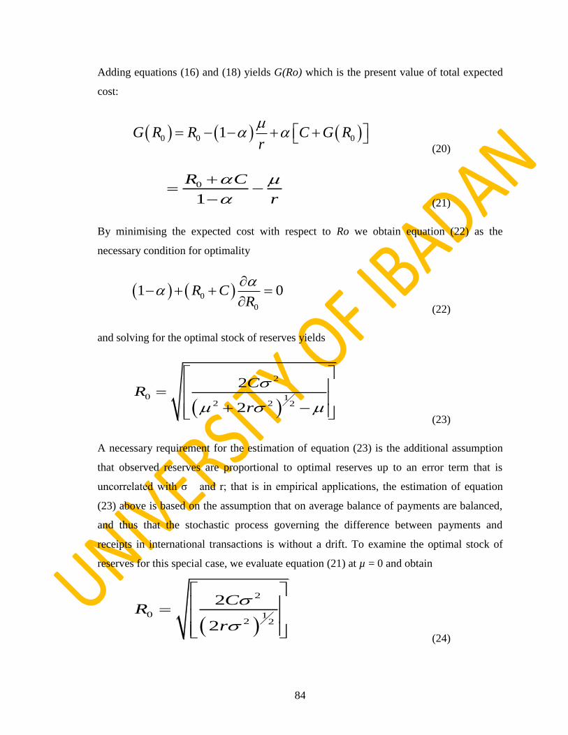
84
Adding equations (16) and (18) yields G(Ro) which is the present value of total expected
cost:
0 0 01G R R C G Rr
(20)
0
1
R C
r
(21)
By minimising the expected cost with respect to Ro we obtain equation (22) as the
necessary condition for optimality
0
0
1 0R CR
(22)
and solving for the optimal stock of reserves yields
2
0 12 2 2
2
2
CR
r
(23)
A necessary requirement for the estimation of equation (23) is the additional assumption
that observed reserves are proportional to optimal reserves up to an error term that is
uncorrelated with σ and r; that is in empirical applications, the estimation of equation
(23) above is based on the assumption that on average balance of payments are balanced,
and thus that the stochastic process governing the difference between payments and
receipts in international transactions is without a drift. To examine the optimal stock of
reserves for this special case, we evaluate equation (21) at µ = 0 and obtain
2
0 12 2
2
2
CR
r
(24)

85
The previous analysis implies that, for the special case of no drift, the optimal level of
reserves is Ro, equation (25), which can be written as:
1 1 1 12 2 2 2
0 2R C r
(25)
which shows reserves as a function of some basic macroeconomic variables
, ,R f C r (26)
or
, , ......R f C r . (27)
In estimable form, equation (23) becomes
In R = β0 + β1ln σ + β2ln r +…+ u (28)
rewritten in order to accommodate other major macroeconomic variables in the
encompassed analytical framework.
4.1.2 The OCA and Asymmetric Shock Model
As noted earlier, the OCA theory [Mundel (1961), McKinnon (1963) Kenan (1969),
Mongeli (2002), Debrun, Masson and Patillo (2005), Ricci (2008)] identifies the sources
of asymmetric shocks to an economy to cover a wide spectrum in the literature. These
include exchange rate variability among members, output variation, variation in terms of
trade and trade flow, and variation in consumer price index. Also in the literature,
asymmetric shocks are traced to fiscal policy distortions resulting from public
expenditure, deficit financing and investment. The asymmetric shock model is shown to
follow a vector autoregressive process where in the initial stage according to Floyd
(2005), a two-variable state of the model and each variable depends on its lagged values,
the current and lagged values of the other variable and on a iid error term is considered as
presented next.
(29) 1( ) 10 12 2( ) 11 1( 1) 12 2( 2) 1( )t t t t ty v v y a y a y e

86
(30)
In matrix notation, this system is written as follows
(31)
However, with K variables and P lags:
(32)
Where yt, v and et are kx1 column vectors and A0, A1, A2, . . . Ap are K x K matrices of
coefficients. The vector et is a vector of white noise residuals that satisfies =
D, where D is a diagonal matrix. An appropriate scaling of the elements of y would make
D an identity matrix.
The standard (reduced) form of the above structural VAR system in equations 29 and 30
can be seen:
(33)
(34)
More compactly,
(35)
2( ) 20 21 1( ) 21 1( 1) 22 2( 2) 2( )t t t t ty v v y a y a y e
1( ) 1( ) 1( 1) 1( )10 12 11 12
21 21 222( ) 20 2( ) 2( 1) 2( )
0
0
t t t t
t t t t
y y y ev v a a
v a ay v y y e
0 1 1 2 2 3 3 ...t t t t t p t p ty v A y A y A y A y A y e
t tE Ee e
1( ) 10 11 1( 1) 12 2( 2) 1( )t t t ty b b y b y u
2( ) 20 21 1( 1) 22 2( 2) 2( )t t t ty b b y b y u
1( ) 1( 1) 1( )10 11 12
21 222( ) 20 2( 1) 2( )
t t t
t t t
y y ub b b
b by b y u

87
Where
(35a)
With
(35b)
And
(35c)
While for the K variable case with p lags,
(36)
With the assumption that the inverse of (I - A0) exists, this reduces to
10 12 2010
12 21
12 11 2111
12 21
12 12 2212
12 21
1
1
1
v v vb
v v
v a ab
v v
a v ab
v v
20 21 1020
12 21
21 21 1121
12 21
21 21 2222
12 21
1
1
1
v v vb
v v
a v ab
v v
v a ab
v v
1( ) 1( ) 12 2( )
12 21
1
1t t tu e v e
v v
2( ) 2( ) 21 1( )
12 21
1
1t t tu e v e
v v
0 1 1 2 2 3 3( ) ...t t t t p t p tI A y v A y A y A y A y e
1 1 1
0 0 1 1 0 2 2( ) ( ) ( )t t ty I A v I A A y I A A y
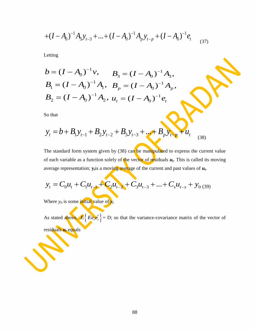
88
(37)
Letting
So that
(38)
The standard form system given by (38) can be manipulated to express the current value
of each variable as a function solely of the vector of residuals ut. This is called its moving
average representation; ytis a moving average of the current and past values of ut.
(39)
Where y0 is some initial value of yt
As stated above, = D; so that the variance-covariance matrix of the vector of
residuals ut equals
1 1 1
0 3 3 0 0( ) ... ( ) ( )t p t p tI A A y I A A y I A e
1
0
1
1 0 1
1
2 0 2
( ) ,
( ) ,
( ) ,
b I A v
B I A A
B I A A
1
3 0 3
1
0
1
0
( ) ,
( ) ,
( )
p p
t t
B I A A
B I A A
u I A e
1 1 2 2 3 3 ...t t t t p t p ty b B y B y B y B y u
0 1 1 2 2 3 3 0...t t t t t s t sy C u C u C u C u C u y
t tE Ee e

89
(40)
However, the problem is that the shocks to the equations contained in the vector utare
correlated with each other. We therefore cannot determine what the effects on the K
variables of a shock to an individual structural equation alone would be. This is so as an
observed utwill represent the combined shocks to a number of equations. This can be seen
from the fact that from equation (40),
(41)
Therefore, in order to determine the effects of a shock to an individual structural equation
of the system, we have to be able to solve the system for A0 and thereby obtaining
. This is vital as it will enable us to operate on equation (39) to transform the
Ut-j‟s into et-j‟s and in the process of doing this, the matrices Cjwill also be transformed
into a useful representation of the impulse responses.
1
0
1 1
0 0
1 1
0 0
1 1
0 0
1 1
0 0
( ) ,
( ) ( )
( ) ( )
( ) ( )
( ) ( )
t t
t t
t t
t t
t t
t t
E Eu u
where
u I A e
E Eu u
E I A e I A e
E I A e e I A
I A E e e I A
I A D I A
1
0( )t tu I A e
1
0( )I A

90
The matrix A0 can be obtained by statistically estimating the structural model (32). If so,
the necessity of running a VAR would have been obviated. However, the reason for VAR
analysis is to avoid multi-equation structural models. The approach used to identify A0 in
VAR analysis is to find the matrix that will orthogonalise the errors; that will transform
the ut-j's in into the et-j's, which are uncorrelated with each other.
Given any matrix G that has an inverse, equation (39) can be rewritten as follows:
(42)
Therefore, the main task here requires finding the G for which
(43)
Then
(44)
Where which implies that
1 1 1
0 1 1 2 2t t t ty C GG u C GG u C GG u
1 1
3 3 0.....t s t sC GG u C GG u y
1
0( )G I A
0 1 1 2 2 3 3 0.....t t t t t s t sy Z e Z e Z e Z e Z e y
1
t j t je G u
t j t ju Ge

91
The Cholesky Decompositions
Since the matrix of coefficient A0is a K x K matrix, it is always of the form,
(45)
Then the structural equation will be of the form
(46)
0 0 0
21 21 21
0 0 0
31 31 31
0 0 0
41 41 41
00 0 0
( 1)1 1 1
0 0 0 0 0
0 0
0 0
0 0
0m mm m m
a a a
a a a
a a a
aa a a
1
1 11 1( 1)
0 1 1
2 21 1 21 1( 1) 22 2( 1)
0 0 1 1
3 31 1 32 2 31 1( 1) 32 2( 1)
0 0 0 1 1
4 41 1 42 2 43 3 42 1( 1) 42 2( 1)
..... ..................................................
t t
t t t t
t t t t t
t t t t t t
y a y
y a y a y a y
y a y a y a y a y
y a y a y a y a y a y
..........................
..... ............................................................................
..... ............................................................................

92
It is worthy of note from the system that none of the current year values of y2, y3,
y4,……,ymenter into the determination of the current year level of y1. The current year
level of y1 enters into the determination of the current year level of y2 and both the current
levels of y1 and y2 enter into the determination of the current level of y3, the current levels
of y1, y2 and y3 enter into the determination of the current level of y4, and so forth so that
the system is fundamentally recursive.
4.2 Methodology
The discussion in the theoretical framework section above gives rise to the following
models. The first is based on the theory of demand for reserves, which leads to the
estimation of the demand and supply determinants of international reserves and the second
is the OCA theory and asymmetric shocks model which dovetails into the evaluation of
reserves pooling and macroeconomic stability.
4.2.1 Model1
Stemming from thecalibration that leads to equations 27 and 28, the external reserves
demand and supply function for international reserves in the ECOWAS region can be
specified as follows:
1 1 1 1 2 3 4 5t it it it it it iRES RES GDPGR EXPT INVT FDI
(47)
and
1 1 1 1 2 3 4 5 6t it it it it it it iRES RES DEBT IMPT GOVT INF EXR
(48)
Where, RESt in the study stands for the total reserves of the individual countries as
percentage of GDP. Reserves here are total reserves minus gold comprising special
drawing rights, reserves of IMF members held by the IMF, and holdings of foreign
exchange under the control of monetary authorities. Gold holdings are excluded. Data are
in current U.S. dollars. GDPGR represents the growth rate of GDP of the countries under
consideration. It is the annual percentage growth rate of GDP at market prices based on
constant local currency. Aggregates are based on constant 2000 U.S. dollars. GDP is the
sum of gross value added by all resident producers in the economy plus any product taxes
93
and minus any subsidies not included in the value of the products. It is calculated without
making deductions for depreciation of fabricated assets or for depletion and degradation of
natural resources.
GOVT is general government final consumption expenditure as percentage of GDP.
General government final consumption expenditure is also general government
consumption which includes all government current expenditures for purchases of goods
and services (including compensation of employees). It also includes most expenditure on
national defense and security, but excludes government military expenditures that are part
of government capital formation.
INV is investment which is measured by gross capital formation as percentage of GDP.
Gross capital formation which is also gross domestic investment consists of outlays on
additions to the fixed assets of the economy plus net changes in the level of inventories.
Fixed assets include land improvements (fences, ditches, drains, and so on); plant,
machinery, and equipment purchases; and the construction of roads, railways, and the like,
including schools, offices, hospitals, private residential dwellings, and commercial and
industrial buildings. Inventories are stocks of goods held by firms to meet temporary or
unexpected fluctuations in production or sales, and "work in progress." According to the
1993 SNA, net acquisitions of valuables are also considered capital formation.
EXPT is exports as percentage of GDP.Exports of goods and services represent the value
of all goods and other market services provided to the rest of the world. They include the
value of merchandise, freight, insurance, transport, travel, royalties, license fees, and other
services, such as communication, construction, financial, information, business, personal,
and government services. They exclude compensation of employees and investment
income (formerly called factor services) and transfer payments. IMPT is imports as
percentage of GDP. Imports of goods and services represent the value of all goods and
other market services received from the rest of the world. They include the value of
merchandise, freight, insurance, transport, travel, royalties, license fees, and other
services, such as communication, construction, financial, information, business, personal,
and government services. They exclude compensation of employees and investment
income (formerly called factor services) and transfer payments.

94
DEBT is total external debt stock as percentage of GDP. It measured as total debt owed to
non-residents repayable in foreign currency, goods, or services. It is the sum of public,
publicly guaranteed, and private nonguaranteed long-term debt, short-term debt, and use
of IMF credit. EXR is the period average official exchange rate of the respective local
currency to the US dollar. It is the exchange rate determined by national authorities or to
the rate determined in the legally sanctioned exchange market. It is calculated as an annual
average based on monthly averages (local currency units relative to the U.S. dollar).
Finally, εt is a vector of innovations that may be contemporaneously correlated but are
uncorrelated with their own lagged values and uncorrelated with all of the right-hand side
variables.
FDI is foreign direct investment as percentage of GDP. It is the net inflows of investment
to acquire a lasting management interest (10 percent or more of voting stock) in an
enterprise operating in an economy other than that of the investor. It is the sum of equity
capital, reinvestment of earnings, other long-term capital, and short-term capital as shown
in the balance of payments. This series shows total net, that is, net FDI in the reporting
economy from foreign sources less net FDI by the reporting economy to the rest of the
world.
INF is inflation rate. Inflation as measured by the consumer price index reflects the annual
percentage change in the cost to the average consumer of acquiring a basket of goods and
services that may be fixed or changed at specified intervals, such as yearly. The Laspeyres
formula is generally used.
4.2.2 Model 2
This study also models the behaviour of the macroeconomic variables identified by the
OCA theory as the sources of macroeconomic shocks with respect to pooled and unpooled
reserves to examine whether a possible reserves pooling arrangement in the ECOWAS
region can mitigate the negative impact of the shocks with the aid of the observed
dynamic impulse responses from the vector autoregressive framework calibrated in
section 4.1 above. The impulse response can provide information on how a variable
responds to shocks or innovations in other variables. Also, it enables us trace temporal
responses of variables to its own shocks and shocks in other variables as well as provide

95
detailed information on the relative strength and stability of the pooling arrangement.
Thus, following the sources of shocks in the OCA theory and the framework in equation
(46), the succeeding behavioural equations are specified:
(49)
(50)
(51)
(52)
(53)
(54)
RESU in the study stands for the total unpooled reserves of the individual countries as
percentage of GDP. Reserves are total reserves minus gold comprising special drawing
rights, reserves of IMF members held by the IMF, and holdings of foreign exchange under
the control of monetary authorities. Gold holdings are excluded. RESP represents pooled
reserves of the countries as percentage of their GDP in the region. This is a situation
where the countries in the region are committed to a 60% reserves pooling arrangement.
Notably, 60% is chosen as it is discovered that this is the prevailing pooling commitment
in the WAEMU as it is considered to be pooling already. Thus this study intends to
employ this commitment to examine the effect of the pooling on macroeconomic stability
for the ECOWAS region. WAEMU‟s pooling is used as a benchmark to do a
counterfactual analysis for ECOWAS on the impact of pooling on macroeconomic
stability of ECOWAS.
1 1
p p
it i t i i t i t
i i
GOVT RESU RESP
1 1
p p
it i t i i t i t
i i
INV RESU RESP
1 1
p p
it i t i i t i t
i i
GDPGR RESU RESP
1 1
p p
it i t i i t i t
i i
TRF RESU RESP
1 1
p p
it i t i i t i t
i i
DEBT RESU RESP
1 1
p p
it i t i i t i t
i i
EXR RESU RESP

96
GDPGR represents the growth rate of GDP of the countries under consideration. It is the
annual percentage growth rate of GDP at market prices based on constant local currency.
Aggregates are based on constant 2000 US dollars. GDP is the sum of gross value added
by all resident producers in the economy plus any product taxes and minus any subsidies
not included in the value of the products. It is calculated without making deductions for
depreciation of fabricated assets or for depletion and degradation of natural resources.
GOVT is general government final consumption expenditure as percentage of GDP.
General government final consumption expenditure is also general government
consumption which includes all government current expenditures for purchases of goods
and services (including compensation of employees). It also includes most expenditure on
national defense and security, but excludes government military expenditures that are part
of government capital formation.
INV is investment which is measured by gross capital formation as percentage of GDP.
Gross capital formation which is also gross domestic investment consists of outlays on
additions to the fixed assets of the economy plus net changes in the level of inventories.
Fixed assets include land improvements (fences, ditches, drains, and so on); plant,
machinery, and equipment purchases; and the construction of roads, railways, and the like,
including schools, offices, hospitals, private residential dwellings, and commercial and
industrial buildings. Inventories are stocks of goods held by firms to meet temporary or
unexpected fluctuations in production or sales, and "work in progress." According to the
1993 SNA, net acquisitions of valuables are also considered capital formation.
TRF represents trade flows as percentage of GDP which is a measure of the degree of
openness of the countries. It consists of the ratio of total exports and import to GDP in
percentage. Here, exports of goods and services represent the value of all goods and other
market services provided to the rest of the world. They include the value of merchandise,
freight, insurance, transport, travel, royalties, license fees, and other services, such as
communication, construction, financial, information, business, personal, and government
services. They exclude compensation of employees and investment income (formerly
called factor services) and transfer payments. Imports of goods and services represent the
value of all goods and other market services received from the rest of the world. They

97
include the value of merchandise, freight, insurance, transport, travel, royalties, license
fees, and other services, such as communication, construction, financial, information,
business, personal, and government services. They exclude compensation of employees
and investment income (formerly called factor services) and transfer payments.
DEBT is total external debt stock as percentage of GDP. It measured as total debt owed to
non-residents repayable in foreign currency, goods, or services. It is the sum of public,
publicly guaranteed, and private nonguaranteed long-term debt, short-term debt, and use
of IMF credit. EXR is the period average official exchange rate of the respective local
currency to the US dollar. It is the exchange rate determined by national authorities or to
the rate determined in the legally sanctioned exchange market. It is calculated as an annual
average based on monthly averages (local currency units relative to the US dollar).
Finally, εt is a vector of innovations that may be contemporaneously correlated but are
uncorrelated with their own lagged values and uncorrelated with all of the right-hand side
variables.
4.3 Estimation Techniques
Panel data analysis will be employed to examine the supply and demand determinants of
international reserves holdings for the countries in the first instance. This will provide an
empirical elucidation on the determinants of international reserves for the region. Here,
both the fixed effects model and the random effects model will be considered. In order to
examine the impact of reserves pooling on ECOWAS macroeconomic stability, the
impulse response and variance decomposition from the vector autoregression (VAR)
framework will be employed. VAR is commonly used for forecasting systems of
interrelated time series and for analysing the dynamic impact of random disturbances on
the system of variables. The VAR approach obviates the necessity for structural modeling
by treating every endogenous variable in the system as a function of the lagged values of
all of the endogenous variables in the system as well as other exogenous variables. It
measures the percentage of the forecast error of variable that is explained by another.
Precisely, it indicates the relative impact that one variable has on another variable. At the
same time, it provides information on how a variable of interest responds to shocks or

98
innovations in other variables. On the other hand, the IRFs allow us to trace temporal
responses of variables to its own shocks and shocks in other variables. The results of the
VDCs will provide detailed information on the relative strength and stability of the
pooling arrangement. From the VDCs and IRFs results, we will capture the relative
importance of various shocks and their influences on the macroeconomic stability of
member states. The VDCs and IRFs are simulated by orthogonalising the innovations in
the VAR equations using the Cholesky decomposition suggested by Sim (1980).
The impulse response is employed to examine the dynamic relationships among variables
specifically in this study among macroeconomic variables in relation to a reserves pooling
arrangement. The impulse response function traces the time path of a shock in one
variable on the remaining variables. By providing the time path of the impact of a shock
on the future values of all the variables in the multivariate dynamic system, the impulse
response analysis should give better insights into short-term and long-term linkages
among the variables employed in each of the six behavioural models employed in this
study. On the other hand, the variance decomposition sequences depict a compact
overview of the dynamic structures of the VAR Model. This decomposition is also based
on a vector moving average model and orthogonal error terms. In contrast to impulse
response, the task of variance decomposition is to generate information about the forecast
ability. The idea is that even a perfect model involves ambiguity about the realisation of
the endogenous variable and its lags because the error terms are associated with
uncertainty. According to the interactions between the equations, the uncertainty is
transformed to all equations. Thus, the aim of the decomposition is to reduce the
uncertainty in one equation to the variance of error terms in all equations.
The choice of this methodology is informed by the fact that when measuring responses to
shocks and instability transmission, the VAR methodology is suitable as evident in
various studies that have made use of the technique (see, Ogunkola 2005, Bayoumi and
Eichengreen, Wami 2005 and Okafor 2011). However, VAR is observed as only a better
tool of measuring shocks which makes it more restrictive as Ogunkola (2005) has pointed
out the relative dearth of appropriate methodology in studies relating to monetary
integration and the OCA criteria.

99
4.4 Data Type and Sources
The study makes use of time series data from 1981 to 2011 (but uses data from 2001-2011
in the first instance of the analysis) obtained from the IMF International Financial
Statistics (IFS) and the World Bank Social Indicators of Development database. Some of
the variables of interest for the models to be used in this study include external reserves,
GDP, exchange rate, inflation, import of goods and services, export of goods and services,
and interest rate.

100
CHAPTER FIVE
EMPIRICAL ANALYSIS
5.1 Data Diagnostics
5.1.1 Summary Statistics
Table 5.1 shows the summary statistics of the macroeconomic variables employed in this
study for the countries in the ECOWAS region. These variables are the unpooled reserves
of the countries (RESU), pooled reserves of the countries under an optimal 60% pooling
arrangement (RESP), government expenditure (GOVT), investment (INV), growth rate of
GDP (GDPGR), trade flow (TRF), debt (debt) and exchange rate (EXR). With the
exception of exchange rate (which is in log) and GDPGR, all the variables employed are
percentage shares of the GDP of the respective countries in US dollars.From this result, it
can be observed that the average percentage of pooled reserves is the highest among the
variables.
This is closely followed by the percentage share of debt in GDP of 122.68%. This shows
the extent to which debt accumulation is a subject of concern in the region with countries
like Liberia, Guinea Bissau and Cote d‟voire with the highest individual average shares of
584.53%, 264.90% and 177.8% respectively. The percentage share of trade flows is the
next highest after debt. This shows the extent to which the countries in the region are
opened in terms of trading activities with other countries of the world. The average shares
of investment, government expenditures and unpooled reserves are 18.44%, 13.24% and
10.41% respectively while of EXR and GDPGR are 4.76 and 3.41% respectively. An
observation of the median values of the variables reveals that they are not significantly
different from their respective mean values except for the share of pooled reserves and
debt.

101
Table 5.1. Summary Statistics of Macroeconomic Variables Employed in the Study
RESU RESP GOVT INV GDPGR TRF DEBT EXR IMP EXP
Mean 10.40509 116.5880 13.24184 18.43927 3.326305 65.10890 122.6810 4.57509 36.5819 24.9884
Median 9.491249 48.58316 11.99950 17.53587 3.783271 61.95884 79.65388 5.70556 33.0692 24.4797
Maximum 50.58917 924.2271 54.51542 52.88038 106.2798 178.9820 1829.488 8.80357 144.616 91.5139
Minimum -0.482653 1.888341 2.851294 -2.424358 -51.03086 6.320343 4.543929 -8.19927 0.00000 0.00000
Std. Dev. 8.360771 168.2401 5.922469 9.349251 8.423420 24.50516 190.1991 2.78816 18.5086 13.4685
Skewness 1.025826 2.590387 1.981421 0.982843 2.736513 0.903235 5.519907 -1.64706 1.20561 0.51011
Kurtosis 4.411807 9.896001 10.90381 4.188519 57.36284 4.578524 40.70880 5.94179 8.20299 3.85671
Jarque-Bera 116.0379 1425.909 1384.336 92.11889 57093.34 104.3107 29590.10 377.917 630.298 34.0172
Probability 0.000000 0.000000 0.000000 0.000000 0.000000 0.000000 0.000000 0.00000 0.00000 0.00000
Sum 4671.886 53630.46 5627.781 7726.052 1526.774 28322.37 56433.27 2127.41 16827.6 11494.6
Sum Sq. Dev 31316.31 12991870 14872.07 36536.75 32496.93 260618.2 16604640 3607.07 157238 83263.1
Observations 460 460 425 429 459 435 460 465 460 460
Source: Author’s Computation from Estimation Results

102
In addition, the standard deviations of the variables are also clustered around the mean
values suggesting that the variables are properly distributed. The standard deviation as
well as the kurtosis and skewness are measures of dispersion.The result suggests that all
the variables are positively skewed safe for exchange rate which has a fat-left tail. The
mean, skewness, kurtosis and Jarque Bera are traditional tests for the establishment of the
normality of the variables. Based on the shown outcomes in the table we reject the null
hypothesis of normal distribution of the variables. The implication of this is that normality
tests statistics such as the t, z and F may not be significantly consequential for drawing
statistical inferences about the probability of the error terms. This finding is further
corroborated by the multivariate VAR residual normality tests and presented in the
appendices.
5.1.2 Panel Unit Root Test
Since the study largely employed time series data, the stationarity properties of the
variables are considered. The test is carried out the results are presented in table 5.2. Here
panel unit root is the focus since the scope of the study is a panel of countries. This is done
using two different types of panel unit root tests. These are the Levin, Lin and Chu test as
well as the Im, Pesaran and Shin test. The tests are carried out to determine the stationarity
level of the variables. From the results using the Levin, Lin and Chu, the variables RESU,
RESP, GOVT, INV, TRF, DEBT and EXR are integrated of order one. GDPGR is the
only variable in the list that is tested to be integrated of order 0. These conclusions are
arrived at on the basis of the critical values denoted beneath the table. These levels of
stationarity of the variable are further corroborated by the results from the Im, Pesaran and
Shin test that the variables, except GDPGR are not integrated at level but integrated at
their respective first differences.

103
Table 5.2. Panel Unit Root Test for the Variables Employed
VARIABLES Levin, Lin & Chu t* Im, Pesaran and
Shin W-stat
Order of
Stationarity
Conclusion
RESU -8.59180 -10.5852 1st Difference I(1)
RESP -10.6370 -10.3981 1st Difference I(1)
GOVT -11.0824 -12.1192 1st Difference I(1)
INV -6.39935 -10.2697 1st Difference I(1)
GDPGR -6.55820 -9.78706 Level I(0)
TRF -9.67387 -11.7141 1st Difference I(1)
DEBT -7.27960 -8.47671 1st Difference I(1)
EXR -6.50336 -8.53900 1st Difference I(1)
Note: the critical values are -3.64, -2.95 and -2.61 for 1%, 5% and 10% significant levels respectively
Source: Author’s Computation from Estimation Results

104
5.1.3 Cointegration Test
Given the non-stationarity properties of the variables evidenced from the unit root test
conducted, the obviation of the possibilities of spuriousness of estimation results is a
necessity. This is done through the determination of the possibility of along run
relationship existing between and among the chosen variables. The possibility of a long
run relation is carried out by the use of cointegration test. In this study, two types of
cointegration tests are carried out. The Kao residual cointegration test and the Johansen
test for multivariate cointegration are also employed to examine the cointegration status of
the six behavioural equations in this part of the study.
i. Panel Cointegration Test
The result from the Kao residual cointegration test is presented in table 5.3.

105
Table 5.3. Panel Cointegration Test
Kao Residual Cointegration Test
Series: RESU RESP GOVT INV GDPGR TRF DEBT EXR
Null Hypothesis: No cointegration
Trend assumption: No deterministic trend
Automatic lag length selection based on SIC with a max lag of 2
Newey-West automatic bandwidth selection and Bartlett kernel
t-Statistic Prob.
ADF -1.631272 0.0414
Residual variance 13.43685
HAC variance 10.52585
Source: Author’s Computation from Estimation Results

106
The Kao test is carried out using an Automatic lag length selection based on Schwartz
information criterion with a maximum lag of two and also on the basis of Newey-West
automatic bandwidth selection and Bartlett Kernel. The assumption regarding the trend is
that of no deterministic trend. The null hypothesis is that of no cointegration among the
variables. From the results reported in table 5.3 on the basis of the Kao residual test, the
null hypothesis of no cointegration can be rejected on the basis of the shown probability
value at 5% level of significance. Therefore, we can accept the alternate hypothesis and
conclude in favour of the presence of cointegration among the chosen variables.
vi. The Johansen Cointegration Test
The Johansen cointegration test results for the behavioural equations are shown in table
5.4below. The table displays the behavioural equations as well as the number of
cointegrating equations found on the basis of the trace test values as well as the max-
eigenvalues. From table 5.4, it can be observed that each of the trace and the max-
eigenvalue detect the presence of two cointegrating equations for the government
equation. This is also the observation for the investment equation where two cointegrating
equations are detected for both the trace and max-eigen value. However, in the economic
growth equation, both the trace and the max-eigenvalue detect the presence of three
cointegrating equations. For the remaining trade flow equation, debt equation as well as
the exchange rate equation, two cointegrating equations are detected by both trace and
max-eigenvalue. This shows that in all the six behavioural equations, we cannot accept the
null hypothesis of no cointegration among the variables but accept the alternate hypothesis
and conclude that there exists the presence of a long run relationship among the variables.
By implication, if a set of variables are cointegrated in econometrics analysis, the effects
of a shock to one variable spread to the others, possibly with time lags, so as to preserve a
long-run relationship between the variables.
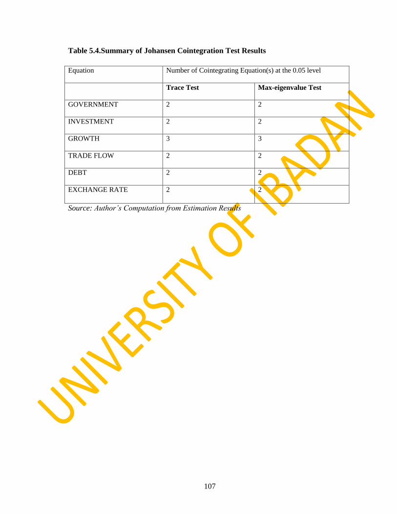
107
Table 5.4.Summary of Johansen Cointegration Test Results
Equation Number of Cointegrating Equation(s) at the 0.05 level
Trace Test Max-eigenvalue Test
GOVERNMENT 2 2
INVESTMENT 2 2
GROWTH 3 3
TRADE FLOW 2 2
DEBT 2 2
EXCHANGE RATE 2 2
Source: Author’s Computation from Estimation Results

108
5.2 Fixed Effects and Random Effects Models for Determinants of
International Reserves in ECOWAS
In the first instance, an analysis of the supply and demand determinants of international
reserves is evaluated for the region. This is a panel data analysis and the fixed effects
model and the random effects models are estimated and examined as presented in table 5.5
below.
It is evident from the results, given the value of the R2
(adjusted), that the independent
variables in the model significantly explain changes in external reserves holdings of the
ECOWAS countries. This is made obvious given the observation that the R2
(adjusted) for
both the fixed effects model (FEM) and random effects model (REM) are 87.9% and
87.7% respectively. Thus, the observable changes in the reserves of the countries are
attributed to the independent variables. The model is overall significant given that the
value of the F-statistic is significant at 1%. The Durbin-Watson statistics for both the FEM
and the REM suggest the null hypothesis that ρ = 0 be accepted where ρ is the
autocorrelation coefficient signifying the absence of serial correlation of the disturbance
term.
From the result of the fixed and random effect models, it can be observed that the results
present sufficient evidence of the impact of the included explanatory variables on the
dependent variable. It is observed that in the fixed effect model, it can be seen that the
constant of the regression is significant albeit at 10%. This shows the value of the
autonomous component of the regression which is the value the dependent variable
assumes in the face of total insignificance of all other independent variables. The random
effect model result however shows that the constant is not significant. The inclusion of the
immediate past period lagged of the dependent variable captures part of the changes in
reserves accumulation in the region as the positive coefficient suggest that the stock of
reserves in time t-1 adds to reserves in time t. Theory, of course, suggests that the value of
a variable in the current period is significantly affected by its lag(s).

109
Table 5.5. Panel Data Analysis of the International Reserves Supply Model for
ECOWAS
Explanatory
variables
Fixed effects model Random effects model
Constant
-0.6807*
(0.6260)
-0.2534
(0.6242)
RESV(-1)
0.8900***
(30.4701)
0.5432*
(2.9436)
GDPGR
0.0033*
(0.0957)
0.8352
(23.263)
INVMT
0.0173**
(0.808)
0.0032*
(5.3621)
INVMT (-1)
-0.0848
(1.932)
-0.3100*
(12.628)
EXPORT
0.0455***
3.4317
0.8912***
(0.3846)
FDI
0.0923**
(1.8745)
0.0085
(0.9860)
Adj. R Square
0.879 0.877
D-Watson
2.1109 1.8946
S.E. of regression
3.2832 3.8725
F- statistic
42.9653***
Hausman Chi-square
- 8.253**
No of
Countries
15 15
Note: (1) The absolute t-statistics are in parentheses. (2) ***, ** and * denote significance at 1%, 5% and
10% levels respectively.

110
This is observed both in the fixed effect model and the random effect models. As
expected, GDP is positively related to reserves hoarding in the region; meaning that GDP
has a significantly positive impact on external reserves accumulation of the country. Even
though the fixed effect model is significant at 1%, the random effect model is not. This
implies that international reserves accumulation increases with economic size in the
ECOWAS region. This result corroborates our apriori expectation about the effect of GDP
on reserves hoarding and as found out in the empirical literatures (Gosselin and Parent,
2005) and (Elhiraika and Ndikumana, 2007) where the effect of GDP on external reserves
is positive and significant.
In support of the main drivers of external reserves discussed earlier, exports of the
countries constitute the major source of supply of the accumulation as evident by the
significance of both the FEM and the REM. This confirms our expectation (apriori)
regarding the effect of this variable as well as the early statement that most African
economies have been accumulating sizable international reserves in the face of today‟s
increasing globalisation and the adverse effect of low reserves holdings during the global
economic crises of 2008. Elhiraika and Ndikumana (2007) confirm this and found further
(by the sizes of their coefficients) that the real exports effect is even greater than the real
GDP effect, underscoring the role of commodity exports (oil and non-oil) in external
reserves buildup among African countries. This result buttresses the significance of
exports in explaining reserves accumulation than GDP.
The result for FDI and net capital inflows is positive and significant at 10% for the FEM
while that of the REM is not significant. As regards the effect and significance of this
variable on the international reserves holdings of the West African economies, the result
reveals is in line with the anticipation of this study that the size of the external reserves
increases with inflow of FDI and capital. Economic theory suggests further that with the
inflow of FDI and capital, there will be adequate provision of employment and
infrastructure thus leading to general alleviation from poverty, thereby obviating the
necessity of de-accumulating the stock of reserves for these purposes. This result also
confirms what Soludo (2007) emphasized concerning the positive impact of the variables
on reserves accumulation of the country.

111
The result with respect to the investment coefficient shows that the variable is significant
in explaining changes in the international reserves holdings of these countries in the
region. As shown, in the current period, the coefficients for both the FEM and the REM
are positive and significant. While the FEM is significant at 5%, the REM is significant at
10%. The first period lag of the variable is included in the analysis as a robustness check.
It is shown that the coefficients are both negative for the FEM and REM models. While
the FEM coefficient is not significant, the REM is significant albeit at 10%. The findings
from the investment result suggest that even though investment may be seen as a dis-
saving in time t-1, current period (thereby leading to the negative relationship observed) it
results to an accretion to overall reserves holdings in the current period. The evidence here
corroborates the result of Elhiraika et al (2007) that investment is seen as a boost to efforts
towards the accumulation of sizable international reserves. Also the results corroborates
the fact that most African economies have been pursuing expansive macroeconomic
policy measures to enable them reap the full benefits of increased public investment in the
future. The Hausman test result rejects the unbiasedness of the random effect model
(estimator) at 5% level of significance which implies that the random effects could be
biased, suggesting the need to somewhat rely solely on the fixed effect model.
Turning attention to the demand model, it is also observed from the results, given the
value of the R2
(adjusted), that the independent variables in the model significantly explain
changes in external reserves holdings of the ECOWAS countries just as it is in the supply
model discussed above. This is made obvious given the observation that the R2
(adjusted)
for both the fixed effects model (FEM) and random effects model (REM) are 86.36% and
85.84% respectively.
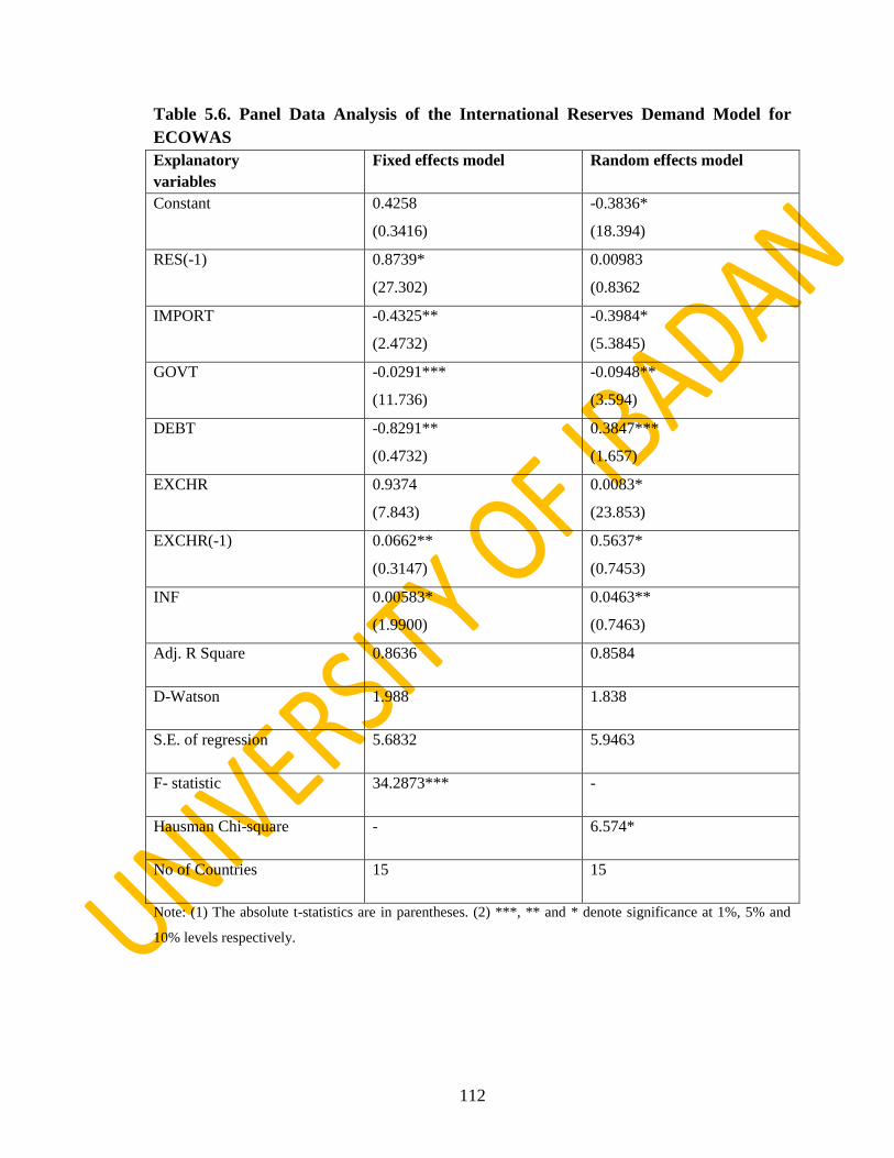
112
Table 5.6. Panel Data Analysis of the International Reserves Demand Model for
ECOWAS
Explanatory
variables
Fixed effects model Random effects model
Constant
0.4258
(0.3416)
-0.3836*
(18.394)
RES(-1)
0.8739*
(27.302)
0.00983
(0.8362
IMPORT
-0.4325**
(2.4732)
-0.3984*
(5.3845)
GOVT
-0.0291***
(11.736)
-0.0948**
(3.594)
DEBT
-0.8291**
(0.4732)
0.3847***
(1.657)
EXCHR
0.9374
(7.843)
0.0083*
(23.853)
EXCHR(-1)
0.0662**
(0.3147)
0.5637*
(0.7453)
INF
0.00583*
(1.9900)
0.0463**
(0.7463)
Adj. R Square
0.8636 0.8584
D-Watson
1.988 1.838
S.E. of regression
5.6832 5.9463
F- statistic
34.2873*** -
Hausman Chi-square
- 6.574*
No of Countries
15 15
Note: (1) The absolute t-statistics are in parentheses. (2) ***, ** and * denote significance at 1%, 5% and
10% levels respectively.

113
Thus, the observable changes in the reserves of the countries are attributed to the
independent variables. The model is overall significant given that the value of the F-
statistic is significant at 1%. The Durbin-Watson statistics, 1.988 and 1.838 for both the
FEM and the REM respectively suggest the null hypothesis that ρ = 0 be accepted where ρ
is the autocorrelation coefficient signifying the absence of serial correlation of the
disturbance term.
The result for both the FEM and REM are as shown in the table. As shown earlier in the
supply model, the inclusion of the immediate past period lagged of the dependent variable
captures part of the changes in reserves accumulation in the region as the positive
coefficient suggest that the stock of reserves in time t-1 adds to reserves in time t which is
in line with the suggestion of theory that the value of a variable in the current period is
significantly affected by its lag(s). This significance is observed in the FEM while the
REM is not. The result shows that the signs of the debt coefficients are negative but for
both the FEM and REM. This is in line with the apriori expectation of this study that the
external debt burden of these ECOWAS countries, in general, depletes the size of reserves
holdings through servicing and principal repayment. Overall, this result is in consonance
with the results of other works that include this variable (Gosselin and Parent, 2005) and
(Elhiraika and Ndikumana, 2007) that there is a negative relationship between external
reserves accumulation and external debt accumulation because external reserves, even
though accumulated, would be depleted for the purpose of servicing accumulated external
debt. The result for imports payment in this study is negative and significant overall for
both the FEM and REM. Among African countries, imports payment is one major variable
responsible for external reserves de-accumulation as most of the country‟s international
outpayments are drawn from this source (Obaseki, 2007). This fact is confirmed by the
negatively significant evidence obtained with regard to the variable as shown in the result
in table 5.6. With respect to the government variable, the result shows that both the FEM
and REM are negative and significant depicting the negative relationship between
government spending and reserves holdings. Just as it is with the import and debt
variables, government spending represents a depletion of reserves holding for the
countries. The governments and monetary authorities of most African economies often
resort to drawing the stock of own reserves to finance domestic spending which include
114
both recurrent like payment of public servants and capital spending such as the
construction of roads and the execution of other developmental projects.
The results for inflation rate and exchange rate exhibit almost the same pattern for both the
FEM and REM. They are both positive though with differing degree of significance in
accounting for changes in reserves position of the countries. The results for these rates are
in consonance with apriori expectations concerning the behaviours of the variables that the
monetary authorities increase international reserves holdings with increased volatilities
and uncertainties of macroeconomic variables. Also, with respect to exchange rate, the
positive coefficients suggest that a rising exchange rate simply implies a depreciation in
nominal terms. This leads to a reduction in the price of exports, a rise in the demand for
exports and an accretion to reserves holdings. The insignificance of exchange rate in the
FEM in the current period in explaining changes in external reserves is in consonance with
result of most studies that include this variable as most studies found out that the variables
are always insignificant in accounting for the behaviour of external reserves as in
Elhiraika and Ndikumana (2007), Choi and Baek (2004), Gosselin and Parent (2005), inter
alia. As expected, reserves rise in the face rising inflation thus, corroborating the result of
Lin and Wang (2005). As it is with the supply model, the Hausman test result reject the
unbiasedness of the random effect model (estimator) at 10% level of significance which
implies that the random effects could be biased, suggesting the need to somewhat rely
solely on the FEM.
5.3 Vector Autoregressive Analysis
An analysis of the possible extent of macroeconomic stability to be achieved when the
countries in the region enter into a reserves pooling arrangement is considered.This is
done primarily using the impulse response function and variance decomposition under the
vector autoregressive framework.
5.3.1 VAR Stability Condition Check Using the Inverse Roots of AR Characteristic
Polynomial
The VAR stability test is conducted to ascertain whether the specification satisfies the
stability condition or not. That is the stability is a way developed in order to verify
whether the VAR model is overall stationary. The implication is that, if the stability

115
condition is violated, then the specifications are not stable, and they are not suitable for
further analysis which would imply non-stability of the VAR specifications. The stability
condition is checked through the use of the inverse roots of AR characteristic polynomial.
The decision rule is that for the specifications to be stable, the characteristic roots of the
polynomial must fall within the unit circle; if all roots of the characteristic AR polynomial
have absolute value less than one. The test is conducted and the result is as shown in
figure 5.1. There should be (number of variables)×(number of model lags) roots visible on
the graph. In this case, we have 16 roots shown which represents the product of the
number of variables and number of optimal lags chosen. The variables employed are
(eight of them) unpooled reserves, pooled reserves, investment, government expenditure,
external debt, GDP, trade flows and exchange rate while the number of model optimal
lags used is gotten to be two. From figure 5.1, it is obvious that all the roots of the
polynomial do not exceed the unit circle; that is all the roots lie inside the circle thereby
fulfilling the stability condition. Given this result, we can conclude that the VAR
specifications are stable.
5.3.2 VAR Residual Tests for Autocorrelations
The VAR residual autocorrelation test is conducted to test the presence (or absence) serial
correlation of the error term. The multivariate Portmanteau and the LM tests are
employed. The null hypothesis that there is “no residual autocorrelations up to lag h” is
tested using both methods and the results presented in table 5.7 and table 5.8. In both
cases, the results from the tests show that the null hypothesis is rejected at 1% significance
level. This suggests that the serial correlation of the residual terms is not a problem

116
Figure 5.1.VAR Stability Test
Source: From Estimation Results
-1.5
-1.0
-0.5
0.0
0.5
1.0
1.5
-1.5 -1.0 -0.5 0.0 0.5 1.0 1.5
Inverse Roots of AR Characteristic Polynomial
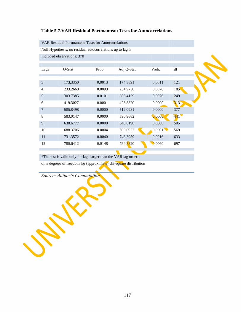
117
Table 5.7.VAR Residual Portmanteau Tests for Autocorrelations
VAR Residual Portmanteau Tests for Autocorrelations
Null Hypothesis: no residual autocorrelations up to lag h
Included observations: 370
Lags Q-Stat Prob. Adj Q-Stat Prob. df
3 173.3350 0.0013 174.3891 0.0011 121
4 233.2660 0.0093 234.9750 0.0076 185
5 303.7385 0.0101 306.4129 0.0076 249
6 419.3027 0.0001 423.8820 0.0000 313
7 505.8498 0.0000 512.0981 0.0000 377
8 583.0147 0.0000 590.9682 0.0000 441
9 638.6777 0.0000 648.0190 0.0000 505
10 688.3706 0.0004 699.0922 0.0001 569
11 731.3572 0.0040 743.3959 0.0016 633
12 780.6412 0.0148 794.3320 0.0060 697
*The test is valid only for lags larger than the VAR lag order.
df is degrees of freedom for (approximate) chi-square distribution
Source: Author’s Computation

118
Table 5.8.VAR Residual LM test for Serial Autocorrelation
VAR Residual Serial Correlation LM Tests
Null Hypothesis: no serial correlation at lag order h
Sample: 1981 2011
Included observations: 370
Lags LM-Stat Prob
1 124.7121 0.0000
2 107.7039 0.0000
3 67.43474 0.0414
Probs from chi-square with 49 df.
Source: Author’s Computation

119
5.3.3 VAR Lag length Selection Criteria
The selection of the lag length is often guided by some criteria. The most commonly
applied are the Akaike information criterion (AIC), the Schwarz information criterion
(SIC) and the Hannan-Quinn information criterion (HQ). From the test results shown in
table 5.9, the AIC and SIC indicate that the appropriate lag length is 2 while the HQ
suggests that the appropriate lag length is 3. Thus, the study adopted the lag length of 2 as
suggested by the AIC and SIC.
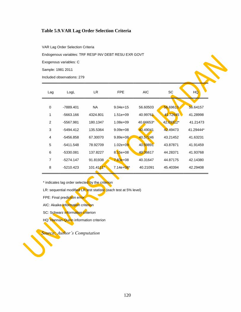
120
Table 5.9.VAR Lag Order Selection Criteria
VAR Lag Order Selection Criteria
Endogenous variables: TRF RESP INV DEBT RESU EXR GOVT
Exogenous variables: C
Sample: 1981 2011
Included observations: 279
Lag LogL LR FPE AIC SC HQ
0 -7889.401 NA 9.04e+15 56.60503 56.69613 56.64157
1 -5663.166 4324.801 1.51e+09 40.99761 41.72645 41.28998
2 -5567.981 180.1347 1.08e+09 40.66653* 42.03312* 41.21473
3 -5494.412 135.5364 9.09e+08 40.49041 42.49473 41.29444*
4 -5456.858 67.30070 9.89e+08 40.57246 43.21452 41.63231
5 -5411.548 78.92709 1.02e+09 40.59891 43.87871 41.91459
6 -5330.081 137.8227 8.15e+08 40.36617 44.28371 41.93768
7 -5274.147 91.81938 7.83e+08 40.31647 44.87175 42.14380
8 -5210.423 101.4111* 7.14e+08* 40.21091 45.40394 42.29408
* indicates lag order selected by the criterion
LR: sequential modified LR test statistic (each test at 5% level)
FPE: Final prediction error
AIC: Akaike information criterion
SC: Schwarz information criterion
HQ: Hannan-Quinn information criterion
Source: Author’s Computation

121
5.3.4 VAR Residual Residual Normality Tests
The VAR normality test is conducted under the null hypothesis that the residuals are
multivariate normal in distribution. From table 5.10, it is observed that the skewness,
kurtosis and Jaque Berra for all the components of the tests are rejected at 5% significance
level. Therefore, the alternate hypothesis is accepted and the conclusion drawn that the
residuals are multivariate normal. This shows that the residual terms of the VAR
specifications are white noise. The implication here is that the VAR model is well
specified and the random terms are purely a result of a random process.

122
Table 5.10. VAR Residual Normality Tests
VAR Residual Normality Tests
Orthogonalization: Cholesky (Lutkepohl)
Null Hypothesis: residuals are multivariate normal
Included observations: 370
Component Skewness Chi-sq df Prob.
1 0.321838 6.387432 1 0.0115
2 0.266637 4.384198 1 0.0363
3 -1.113730 76.49103 1 0.0000
4 0.458984 12.99107 1 0.0003
5 -0.870736 46.75450 1 0.0000
6 0.029101 0.052224 1 0.0492
7 0.973509 58.44276 1 0.0000
8 1.877633 217.4063 1 0.0000
Joint 422.9095 8 0.0000
Component Kurtosis Chi-sq df Prob.
1 4.896442 55.44594 1 0.0000
2 12.01118 1251.855 1 0.0000
3 41.16432 22454.61 1 0.0000
4 6.916335 236.4559 1 0.0000
5 14.72964 2121.095 1 0.0000
6 8.144026 407.9404 1 0.0000
7 9.221809 596.7932 1 0.0000
8 12.74907 1465.267 1 0.0000
Joint 28589.46 8 0.0000
Component Jarque-Bera df Prob.
1 61.83338 2 0.0000
2 1256.240 2 0.0000
3 22531.10 2 0.0000
4 249.4470 2 0.0000
5 2167.849 2 0.0000
6 407.9926 2 0.0000
7 655.2360 2 0.0000
8 1682.673 2 0.0000
Joint 29012.37 16 0.0000
Source: Author’s Computation

123
5.3.5 Impulse Response Analysis
Impulse responses trace out the response of current and future values of each of the
variables to a unit increase in the current value of one of the VAR structural errors,
assuming that this error returns to zero thereafter. The impulse response function is a
practical way of representing the behaviour over time of z in response to shocks to the
vector u. The impulse response is performed in order to examine the impact of reserves
pooling on macroeconomic stability. This is done by appraising the behaviour of some
important macroeconomic variables to shocks arising from unpooled reserves as well as
pooled reserves in the region. The selected macroeconomic variables are investment,
government expenditure, external debt, trade flows, GDP and exchange rate. The analysis
is done over a period of time, in this case, 20 years period. The stability of the
macroeconomic variables is examined through the dynamic effect of a
Choleskynonfactorized one standard deviation innovation from both unpooled and pooled
reserves. The results are presented in what follows.
Response of Government to Innovation from International Reserves
The impulse response of government expenditure from a shock to unpooled reserves
shows an overall significant fluctuation across both the positive and negative domains. As
observed in figure 5.2, a one Cholesky standard deviation shock to unpooled reserves
leads to an initial significant upswing in government spending from the steady state level
of 0.00; it rises and stays approximately 3.7% above the steady state level. Immediately
after this sharp rise, there is an improvement as the disequilibrium starts dwindling from
the 2nd
period and returns to the equilibrium locus in the 7th
period. However, this return is
short-lived as a deterioration is recorded and this deterioration intensifies steadily below
the equilibrium level and extends beyond the end period of the analysis, the 20th
period.
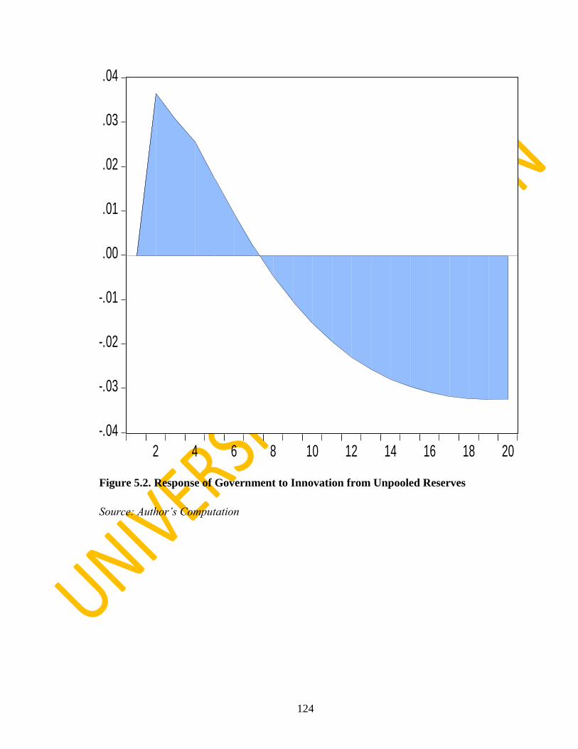
124
Figure 5.2. Response of Government to Innovation from Unpooled Reserves
Source: Author’s Computation
-.04
-.03
-.02
-.01
.00
.01
.02
.03
.04
2 4 6 8 10 12 14 16 18 20

125
Figure 5.3. Response of Government to Innovation from pooled Reserves
Source: Author’s Computation
-.04
-.03
-.02
-.01
.00
.01
.02
.03
.04
2 4 6 8 10 12 14 16 18 20

126
Therefore, for government spending, a positive response from the equilibrium is observed
from period 1 to period 7 and a negative response is observed from the 7th
period till the
20th
as a result of a Cholesky one standard deviation positive shock to the unpooled
reserves of the countries.
On the other hand, one Cholesky standard deviation shock to pooled reserves leads to an
initial infinitesimal deterioration in government spending from the steady state level of
0.00 as shown in figure 5.3. This reaches the peak at about 0.5% and the disequilibrium
peters out immediately in the 5th
period. The impulse response immediately crosses the
steady state locus and takes a steady upswing. It rises and peaks approximately 1% above
the steady state level between the 14th
and 17th
periods. Apart from the fact that the
disequilibrium and response to shock is minimal here, there is a slight evidence of a return
to equilibrium towards the end period.
Response of Investment to Innovation from International Reserves
The impulse response of investment from a shock to unpooled reserves shows a
significant upsurge, purely in the positive domain. This is depicted in figure 5.4. A one
Cholesky standard deviation shock to unpooled reserves leads to a continuous upswing in
investment and reaches its peak in the 11th
period. This peak is approximately 15% above
the equilibrium locus. Immediately after this sharp rise, there is an improvement as the
disequilibrium starts dwindling from the 11nd
period.
Notably, this disequilibrium still remains high even at the end of the 20th
period at
approximately 11%, representing a 26.7% downswing from the peak observed in the 11th
period.
Figure 5.5 shows the impulse response of investment to a one Cholesky standard deviation
shock to pooled reserves.

127
Figure 5.4. Response of Investment to Innovation from Unpooled Reserves
Source: Author’s Computation
.00
.02
.04
.06
.08
.10
.12
.14
.16
2 4 6 8 10 12 14 16 18 20

128
Figure 5.5. Response of Investment to Innovation from pooled Reserves
Source: Author’s Computation
.00
.02
.04
.06
.08
.10
.12
.14
.16
2 4 6 8 10 12 14 16 18 20

129
From the figure, it can be observed that the shock causes investment to shift from its
equilibrium position by an infinitesimal percentage in relation to that of the unpooled
reserves. Starting from the initial period, investment jumps approximately to 1.8%. From
the 2nd
period, the response is apparently constant throughout the forecast period. Overall,
the impact is positive and shift from equilibrium is marginal representing about 88%
lower than the peak under the unpooled reserves. This shows considerable convergence
toward equilibrium in the case of the pooled reserves when compared with the
unpooledreserves counterpart in figure 5.4.
Response of Trade Flows to Innovation from International Reserves
Similar to the response of government expenditure, trade flows show an overall significant
fluctuation across both the positive and negative domain in response to a shock
tounpooled reserves. In figure 5.6, a one Cholesky standard deviation shock to unpooled
reserves leads to an initial significant downswing in trade flows from the steady state level
of 0.00. The swing below the steady state locus reaches its peak in the 2nd period which is
approximately 13% below. Soon after this deterioration, there is an immediate return to
equilibrium corresponding to the 4th
period.
The return is short-lived as a surfeit is which intensifies steadily above the equilibrium
level. It reaches its peak in the 11th
period corresponding to 12% rise above the equilibrium
locus which extends beyond the end period of the analysis, the 20th
period even though
there is a sign of a gradual return to equilibrium, this return however is not within the
period captured by this analysis.

130
Figure 5.6.Response of Trade Flows to Innovation from Unpooled Reserves
Source: Author’s Computation
-.12
-.08
-.04
.00
.04
.08
.12
2 4 6 8 10 12 14 16 18 20

131
Figure 5.7. Response of Trade Flows to Innovation from pooled Reserves
Source: Author’s Computation
-.12
-.08
-.04
.00
.04
.08
.12
2 4 6 8 10 12 14 16 18 20

132
Therefore, with regards to the trade flows analysis, a negative response from the
equilibrium is observed from period 1 to period 4 and a positive response above the
equilibrium is observed from the 7th
period till the 20th
as a result of a Cholesky one
standard deviation positive shock to the unpooled reserves of the countries.Under a
reserves pooling arrangement, the response of trade flows to a shock appear negligible.
Even though there is fluctuation across both the positive and negative domain, the
fluctuationis infinitesimal. From figure 5.7, it is observed that the shock causes trade flow
to shift from its equilibrium position by an infinitesimal percentage in relation to its
impulse response from unpooled reserves. Starting from the initial period, investment
jumps approximately to 1.0%. From the 2nd
period, the response peters out gradually with
a steady return to equilibrium approximately around the 11th
period. Overall, the impact
oscillates across the two domains; positive from the 1st to the 11
th period then negative
from the 11th
period to the end of the 20th
period and shift from equilibrium is marginal
representing about 92% lower than the peak under the unpooled reserves figure above.
This shows considerable convergence toward equilibrium in the case of the pooled
reserves when compared to the unpooled reserves counterpart in figure 5.6.
Response of Gross Domestic Product to Innovation from International Reserves
GDP shows an overall significant fluctuation entirely the positive domain in response to a
shock tounpooled reserves.
In figure 5.8, a one Cholesky standard deviation shock to unpooled reserves exerts about
5% initial significantly positive shock impulse response or innovation in GDP from the
steady state level of 0.00. This initial upswing of about 5% is the peak after which the
shock started diminishing in the 3rd
period equivalent to about 3% and diminishes further
towards to about 2.5% in the 4th
and this remains almost the same till the end of the period
in the 20th
year.

133
Figure 5.8. Response of GDP to Innovation from Unpooled Reserves
Source: Author’s Computation
.00
.01
.02
.03
.04
.05
.06
2 4 6 8 10 12 14 16 18 20

134
Figure 5.9. Response of GDP to Innovation from pooled Reserves
Source: Author’s Computation
.00
.01
.02
.03
.04
.05
.06
2 4 6 8 10 12 14 16 18 20

135
With regards to the GDP analysis, an overall positive response from the equilibrium is
observed throughout the entire period of the analysis with the peak of the shock in the 3rd
period corresponding to 5% as a result of a Cholesky one standard deviation positive
shock to the unpooled reserves of the countries.
Figure 5.9 shows the response of economic growth proxied by GDP here to a one
Cholesky standard deviation shock in pooled reserves. From the figure, it can be observed
that the shock causes investment to shift from its equilibrium position by an infinitesimal
percentage in relation to that of the unpooled reserves. The initial shock response or
innovation exerted upon GDP as a result of a positive shock to pooled reserves is a
positive movement away from steady state. A steady initial rise is observed between
period 1 and 3 where the peak is attained in the 3rd
period through the 4th
to the 6th
period
corresponding to about 0.05% innovation. From thence, the shock response starts to
diminish until the end of the period. Overall, the impact is positive and shift from
equilibrium is marginal where the peak here (of 0.05%) is more than 95% lower than the
peak of the shock response in unpooled reserves. This shows considerable convergence
towards equilibrium in the case of the pooled reserves when compared to the unpooled
reserves counterpart in figure 5.8.
Response of External Debt to Innovation from International Reserves
In the case of debt, there is an overall significant fluctuation entirely in the negative
domain in response to a shock to unpooled reserves. As shown in figure 5.10, a Cholesky
one standard deviation positive shock to unpooled reserves exerts about 6.9% initial
significantly negative shock response or innovation in debt from the steady state level of
0.00. This initial downswing below the equilibrium locus of about 6.9% is the peak and
this peak is attained in the 2nd
period. Soon after this summit, the shock started
diminishing gradually and reached its lowest point in the 10th
through the 13th
period
corresponding approximately to 1% and then the deterioration started getting stronger
from there until the end of the period. Thus, with regards to the debt analysis, an overall
negative response from the equilibrium is observed throughout the entire period of the
analysis with the peak of the shock attained in the 2rd
period corresponding to about 6.9%

136
as a result of a Cholesky one standard deviation positive shock to the unpooled reserves of
the countries. The response of debt to a one Cholesky standard deviation shock in pooled
reserves is represented in figure 5.11. Just as in the case of unpooled reserves, the
oscillation here also is purely in the negative domain in response to a shock to pooled
reserves.
As shown in figure 5.11, a one Cholesky standard deviation shock to pooled reserves
elicited a smooth deterioration in debt, almost u-shaped with the lowest point attained in
the 11th
period corresponding to about 2.4% below the equilibrium locus. Soon after this
lowest point a gradual movement towards equilibrium is observed until the end of the
period where the impact is still approximately 1.8% below the equilibrium. Overall, the
impact is negative and the shift from equilibrium is lower as compared to the
corresponding case of unpooled reserves where the peak here of approximately 2.4% is
about 65% lower than the peak of the shock response in unpooled reserves. On the
average, this shows considerable convergence towards equilibrium.

137
Figure 5.10. Response of External Debt to Innovation from Unpooled Reserves
Source: Author’s Computation
-.7
-.6
-.5
-.4
-.3
-.2
-.1
.0
2 4 6 8 10 12 14 16 18 20

138
Figure 5.11. Response of External Debt to Innovation from pooled Reserves
Source: Author’s Computation
-.7
-.6
-.5
-.4
-.3
-.2
-.1
.0
2 4 6 8 10 12 14 16 18 20

139
Response of Exchange Rate to Innovation from International Reserves
The case of exchange rate, just like that of debt above, shows that the fluctuation is
entirely in the negative domain in response to a shock to unpooled reserves (figure 5.12).
A one Cholesky standard deviation shock to unpooled reserves elicits a continuous
explosion in terms of impulse response in the exchange rate of the countries. There is an
initial jump between the 1st and the 3
rd period; thereafter, there is a steady deterioration in
exchange rate till the end of the period.
At the peak, which happens to the last period in this analysis, it is observed that a shock to
unpooled reserves exerts approximately 1.3% negative shock response or innovation in
exchange rate from the steady state level of 0.00.
The case of the response of pooled reserves is even more interesting as it is almost non-
existent given its infinitesimal representation. As shown in the figure 5.13, the response of
exchange rate to a one Cholesky standard deviation shock in pooled reserves is a paltry
deterioration within the period of the forecast. As a diminutive representation of the
unpooled reserve case above, the shock impulse response here is a continuous slide away
from the equilibrium. At its peak which happens to be the period-end, if the shock in
pooled reserves changes by one Cholesky standard deviation, the impulse or innovation in
exchange rate will respond by approximately 0.1% which is about 92% lower than the
peak of the shock response in exchange rate in the case of unpooled reserves. This shows
considerable convergence towards equilibrium in the case of the pooled reserves as
compared to the unpooled reserves counterpart in figure 5.12.

140
Figure 5.12. Response of Exchange Rate to Innovation from Unpooled Reserves
Source: Author’s Computation
-.014
-.012
-.010
-.008
-.006
-.004
-.002
.000
2 4 6 8 10 12 14 16 18 20
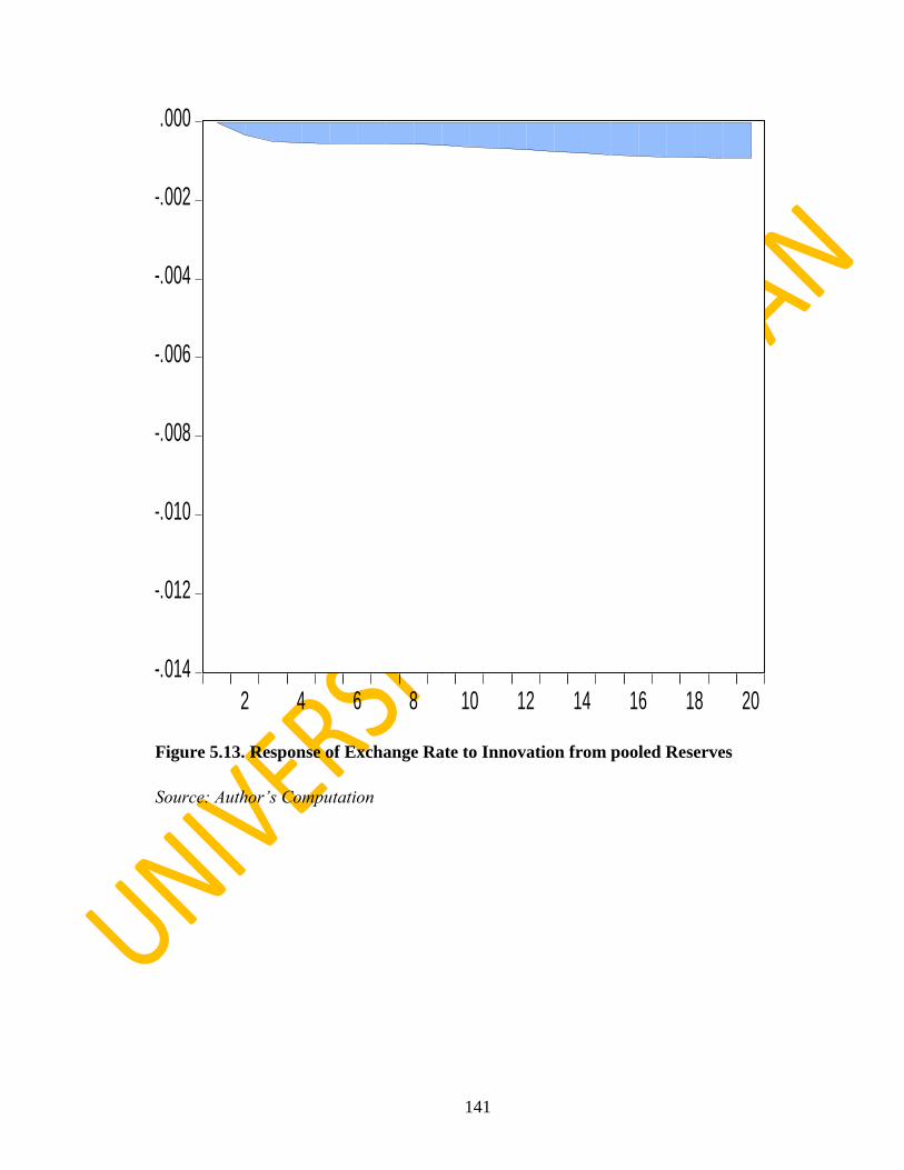
141
Figure 5.13. Response of Exchange Rate to Innovation from pooled Reserves
Source: Author’s Computation
-.014
-.012
-.010
-.008
-.006
-.004
-.002
.000
2 4 6 8 10 12 14 16 18 20

142
5.3.6 Variance Decomposition
The dynamic response of the macroeconomic stability as given in the impulse response
can further be explained by the forecast variance error otherwise known as variance
decomposition. While impulse response functions trace the effects of a shock to one
endogenous variable on to the other variables in the PVAR, variance decomposition
separates the variation in an endogenous variable into the component shocks to the PVAR.
In other words, the variance decomposition provides information about the relative
importance of each random innovation in affecting the variation of the variables in the
PVAR.The summary of the results of the variance decomposition is presented in table
5.11 while the comprehensive decomposition is shown in the appendices. It shows the
percentage of the forecast error variance due to each shock in the PVAR model over the
20 years horizon for the ECOWAS region.
From the results obtained, it is observed that the selected variables are explained to a large
extent by its own shocks when seen over the entire 20 years period of the forecast. On the
basis of their respective averages, it is observed that government expenditure account for
about 95.9% of the random shock response or innovation; investment accounted for about
87.37% of the shock response; GDPGR, trade flows, debt and exchange rate account on
the average 92.36%, 76.18%, 90.67% and 91.14% respectively of the random shock
innovations in each of the behavioural models they represent. It is generally observed that
the degree of responses of the selected macroeconomic variables to shocks from reserves
(pooled and unpooled) is significantly large. Thus in the light of this result, the extent to
which the correction of the distortions and disequilibrium (adjustment back to steady
state) in the region can be costly is greatly reduced. For the Cholesky variance
decomposition, the ordering of the variables can be very important. Thus, the study re-
conducted variance decomposition test to check whether reversing the ordering of the
variables can significantly affect the result obtained.

143
Table 5.11 Variance Decomposition (Summary)
GOVT INV GDPGR TRF DEBT EXR
98.92 99.76 96.48 89.48 85.87 99.82
99.18 98.79 94.39 87.53 91.38 99.08
99.30 97.86 94.04 85.70 94.05 98.27
99.29 96.77 93.64 83.97 95.44 97.37
99.17 95.60 93.26 82.34 95.98 96.40
98.93 94.34 92.93 80.78 95.89 95.37
98.58 92.99 92.64 79.31 95.33 94.31
98.11 91.57 92.40 77.92 94.47 93.24
97.56 90.08 92.19 76.61 93.43 92.19
96.94 88.55 92.00 75.39 92.35 91.16
96.27 86.98 91.84 74.25 91.30 90.17
95.57 85.39 91.69 73.20 90.32 89.23
94.85 83.81 91.56 72.23 89.44 88.34
94.14 82.23 91.44 71.34 88.65 87.51
93.44 80.69 91.33 70.53 87.94 86.72
92.76 79.18 91.23 69.79 87.32 85.99
92.11 77.73 91.14 69.12 86.76 85.30
91.49 76.33 91.06 68.52 86.27 84.66
90.92 75.00 90.99 67.99 85.82 84.06
90.38 73.74 90.92 67.51 85.41 83.51
Source: Author’s Computation from Estimation Results

144
As noted in the table, the endogenous variables represented in the behavioural models:
Government, investment, GDP growth, trade flows, and exchange rate account with
average values 95.9%, 87.37%, 92.36%, 76.18%, 90.67% and 91.14% respectively
accounted for (on an average) 89.0% of the forecast random shock response or
innovations over the 20 years forecast period. However, when the ordering of these
variables is completely reversed, the values are respectively 95.34%, 88.07%, 94.26%,
94.19%, 85.31% and 92.36 averaging 91.91%. as shown in the appendix Difference is
considered to be insignificance to influence major conclusions.
5.4 Analysis of Stability Gained from Reserves Pooling
This study is further extended to evaluate, in quantitative terms, the amount of possible
stability to be gained from the 60% reserves pooling arrangement by the countries in the
community over the 20-years period considered in the study. This is generated from the
impulse response estimation.The result is shown in table 5.12.The first column contains
the list of the macroeconomic variables representing the behavioural equations estimated
in the study. The second and third columns show the estimated instability from unpooled
and pooled reserves respectively. They are calculated as the standard deviation of the
impulse response tabular values obtained for each of the behavioural equations considered
in the study. As shown earlier, the impulse response measures the average
perturbation/response of a variable from its equilibrium state as a result of a shock to
another. The fourth column estimates the stability achieved by the economic community
as a result of a reserve pooling arrangement among the countries. It is defined as the ratio
of the difference between the respective unpooled reserves and the pooled reserves to the
unpooled reserves while the last column is all about the percentage stability gained from
the pooling arrangement.
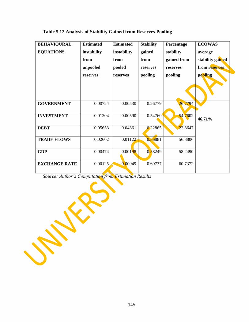
145
Table 5.12 Analysis of Stability Gained from Reserves Pooling
BEHAVIOURAL
EQUATIONS
Estimated
instability
from
unpooled
reserves
Estimated
instability
from
pooled
reserves
Stability
gained
from
reserves
pooling
Percentage
stability
gained from
reserves
pooling
ECOWAS
average
stability gained
from reserves
pooling
GOVERNMENT 0.00724 0.00530 0.26779 26.7794
46.71%
INVESTMENT 0.01304 0.00590 0.54760 54.7602
DEBT 0.05653 0.04361 0.22865 22.8647
TRADE FLOWS 0.02602 0.01122 0.56881 56.8806
GDP 0.00474 0.00198 0.58249 58.2490
EXCHANGE RATE 0.00125 0.00049 0.60737 60.7372
Source: Author’s Computation from Estimation Results

146
From the table, it is observed that the instability to the economy arising from government
spending is 0.00724 when the countries are operating individually - under an independent
state; however, under reserves pooling arrangement, the instability can be reduced to
0.0053. This represents about 26.78% overall stability gained as a result of reserves
pooling relative to the unpooled state of affairs. For investment, it is observed that the
instability under an autonomous state is 0.01304 while it is reduced to 0.0059 under a
pooling arrangement; representing about 54.76% overall improvement in the region. The
external debt record the lowest improvement from a possible reserves pooling
arrangement in the region with 22.86% where the estimated instability from unpooled
reserves is 0.05653 while that from the pooled reserves to 0.0436. With a reserves pooling
arrangement, the stability from trade flows shows a significant improvement compared to
that when the countries are operating autonomously. For the trade flow, the estimated
instability from unpooled reserves is seen to be 0.026 while that under a pooling
arrangement is 0.01122, representing about 56.88% stability gain for the region. The index
of economic growth, GDP, is another area where significant stability will be recorded
when the region is under a reserves pooling arrangement. Here, the estimated instability
for the unpooled scenario is 0.00474 while that for the pooled is 0.00198, representing
about 58.25% improvement and stability compared to the autonomous state of affairs.
From this table, the largest gain is shown to be coming from exchange rate coordination.
Under an unpooled scenario, the estimated instability here is shown to be 0.00125 while
that under pooling is 0.00049. This represents about 60.74% improvement. The overall
average stability gain for the region is computed to be 46.71% when the countries agree
on a 60% reserves pooling. Thus, the study finds strong evidence of macroeconomic
stability as a result of international reserves pooling.
147
5.5 Interpretations
The foregoing analysis considers the response of macroeconomic variables to reserves
under a non-pooling scenario as well as under pooling. It is observed from the results
presented that when there is a shock emanating from reserves and the total reserves are not
adequate enough to insulate the economy, there would be a significant distortion
(disequilibrium) to the economy as shown by the response of the macroeconomic
variables thus the stability of the economy is undermined as a result of this shock and this
creates disequilibrium. However, it is observed from the results presented that when the
countries enter into a reserves pooling arrangement and the reserves available to each
country is significant, the economy is to a large extent insulated from the negative impact
of the shock. It is shown in the results presented that in the cases of pooled reserves
analyzed, the distortion in the economy (in terms of the macroeconomic variables
examined) is infinitesimal in comparison to the distortion to the economy when the
countries are operating in an autonomous state.
From the stability gain analysis carried out, it is observed that the macroeconomic stability
in the region is going to improve under a reserves pooling arrangement for all the
macroeconomic variables selected for this study. It is shown that the lowest stability gain
is recorded by external debt while the highest stability gain is recorded in the area of
exchange rate coordination. This corroborates apriori expectations as under a reserves
pooling arrangement, a large percentage of reserves is often deployed for the stabilization
of the exchange rate. This would be the case under a single currency operation; so that the
exchange rate fluctuation does not overshoot or undershoot the level necessary for the
attainment of the prime goal of macroeconomic stability. Thus, the crux of this study is
the overall estimated macroeconomic stability to be gained if the countries in the region
are to operate under a reserves pooling arrangement. This is estimated to be 46.71% which
is a significant stability gain to be recorded. Overall, it is observed from the study that
reserves are expected to be sources of insulation to the economies so that a positive shock
to reserves should not translate to the economy and deteriorate macroeconomic variables.
However, due the inadequacy of reserves in these countries, it is observed from the
analysis that a positive shock to unpooled reserves drifts the macroeconomic variables
away from d steady state. However, under a pooling arrangement, the instabilities are

148
greatly reduced. This result is significant for the region especially in the face of the
increasing campaign for monetary integration and the contemplation for the adoption of a
single currency in the region.
The finding from this analysis is consistent with the findings of Ogunkola (2005),
Ogunkola and Jerome (2005), Jerome (2005) and Iyoha (2003). These studies find out that
monetary integration could be beneficial to the ECOWAS region even though the
approaches differ.
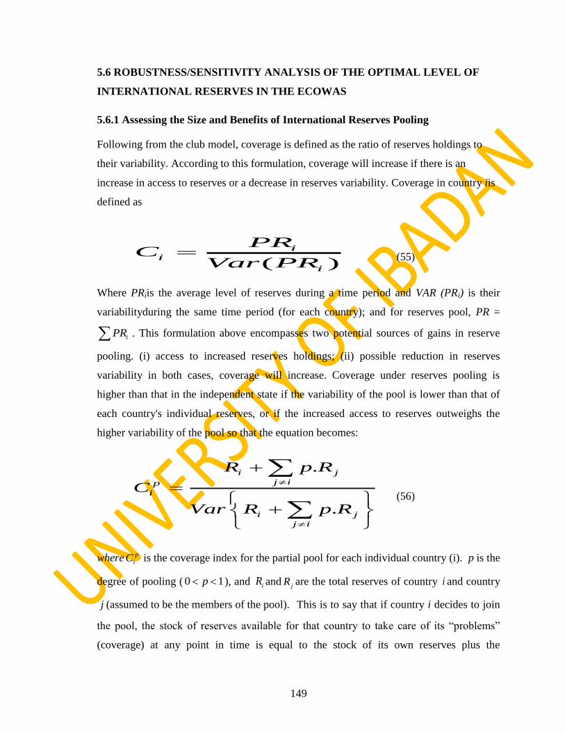
149
5.6 ROBUSTNESS/SENSITIVITY ANALYSIS OF THE OPTIMAL LEVEL OF
INTERNATIONAL RESERVES IN THE ECOWAS
5.6.1 Assessing the Size and Benefits of International Reserves Pooling
Following from the club model, coverage is defined as the ratio of reserves holdings to
their variability. According to this formulation, coverage will increase if there is an
increase in access to reserves or a decrease in reserves variability. Coverage in country iis
defined as
(55)
Where PRiis the average level of reserves during a time period and VAR (PRi) is their
variabilityduring the same time period (for each country); and for reserves pool, PR =
. This formulation above encompasses two potential sources of gains in reserve
pooling. (i) access to increased reserves holdings; (ii) possible reduction in reserves
variability in both cases, coverage will increase. Coverage under reserves pooling is
higher than that in the independent state if the variability of the pool is lower than that of
each country's individual reserves, or if the increased access to reserves outweighs the
higher variability of the pool so that the equation becomes:
(56)
where is the coverage index for the partial pool for each individual country (i). is the
degree of pooling ( ), and and are the total reserves of country and country
(assumed to be the members of the pool). This is to say that if country i decides to join
the pool, the stock of reserves available for that country to take care of its “problems”
(coverage) at any point in time is equal to the stock of its own reserves plus the
( )
ii
i
PRC
Var PR
iPR
.
.
i j
j ip
i
i j
j i
R p R
C
Var R p R
p
iC p
0 1p iRjR i
j
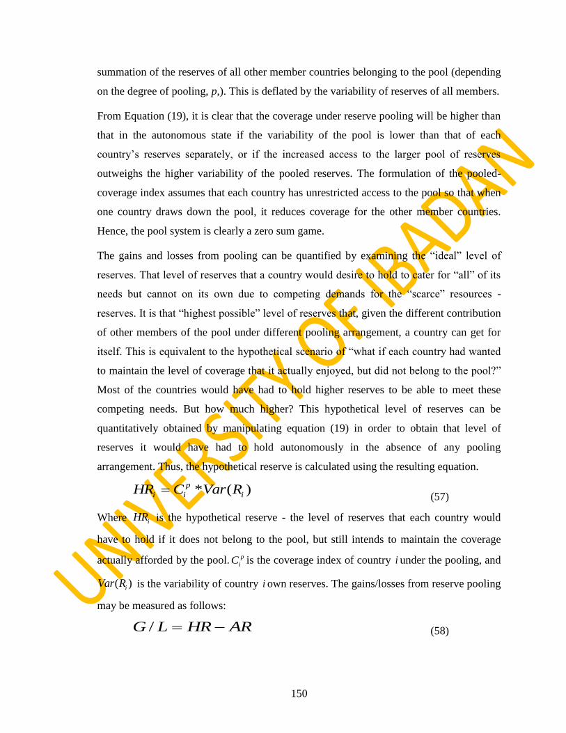
150
summation of the reserves of all other member countries belonging to the pool (depending
on the degree of pooling, p,). This is deflated by the variability of reserves of all members.
From Equation (19), it is clear that the coverage under reserve pooling will be higher than
that in the autonomous state if the variability of the pool is lower than that of each
country‟s reserves separately, or if the increased access to the larger pool of reserves
outweighs the higher variability of the pooled reserves. The formulation of the pooled-
coverage index assumes that each country has unrestricted access to the pool so that when
one country draws down the pool, it reduces coverage for the other member countries.
Hence, the pool system is clearly a zero sum game.
The gains and losses from pooling can be quantified by examining the “ideal” level of
reserves. That level of reserves that a country would desire to hold to cater for “all” of its
needs but cannot on its own due to competing demands for the “scarce” resources -
reserves. It is that “highest possible” level of reserves that, given the different contribution
of other members of the pool under different pooling arrangement, a country can get for
itself. This is equivalent to the hypothetical scenario of “what if each country had wanted
to maintain the level of coverage that it actually enjoyed, but did not belong to the pool?”
Most of the countries would have had to hold higher reserves to be able to meet these
competing needs. But how much higher? This hypothetical level of reserves can be
quantitatively obtained by manipulating equation (19) in order to obtain that level of
reserves it would have had to hold autonomously in the absence of any pooling
arrangement. Thus, the hypothetical reserve is calculated using the resulting equation.
(57)
Where is the hypothetical reserve - the level of reserves that each country would
have to hold if it does not belong to the pool, but still intends to maintain the coverage
actually afforded by the pool. is the coverage index of country under the pooling, and
is the variability of country own reserves. The gains/losses from reserve pooling
may be measured as follows:
(58)
* ( )p
i i iHR C Var R
iHR
p
iC i
( )iVar R i
/G L HR AR

151
Where( ) is the gain (+) or loss (-) in reserve level, and and are the
hypothetical and actual average reserve respectively.
The average reserve holdings for each country and their variability during the scope of the
study will be used. Based on this data, and for each country, we will first compute the
coverage index without pooling (0 percent) and then simulate the country‟s coverage
index by imposing additional 10 percent increments in the level of pooling commitment
(from 10 percent pooling to 100 percent pooling). The highest overall average for the
coverage index with pooling will be found. With this methodology, the level of pooling
that will most benefit the ECOWAS economies as a group will be determined. The
simulation will identify the degree of pooling (whether partial pooling or complete 100%
pooling) that will maximize the overall gains for the countries in the sub-region. Similarly,
this same methodology is employed to examine the case of reserves pooling for the
WAEMU and non-WAEMU zones separately to examine which zones would enjoys
relatively greater gains (or suffer greater loss) from pooling.
5.6.2 Evaluation of Gains/Losses from Reserves Pooling in ECOWAS
This section of the study considers reserves pooling among the ECOWAS countries based
on the average reserves of these respective countries in the last decade (2001-2011). The
choice of this scope is due to the fact that economic transformations in these countries in
the last decade paint a more vivid picture of their present economic realities than periods
in the far past. Thus, reserves positions as well their respective variabilities in the recent
past are assumed to tell more stories about the economies‟ present state of affairs26
. When
a group of countries pool reserves together, each member has an unrestricted access to the
pool. This is one of the major sources of gains. The average reserves of each member
country of ECOWAS and different degrees of pooling for the period 2001 and 2011 are
shown in table 5.13.
26
An alternative analysis using the average reserves of the countries (not reported here) for the entire study
sample scope of three decades (1981-2011) did not produce a vivid picture of the actual average reserves
position of the countries as compared to the results within one decade. In addition, the 1981-2011 sample
periods produced a much lower coverage index of reserves pooled for the region.
/G L HR AR

152
With reserves pooling, a country‟s reserves equals its own total reserves holding plus the
sum of partially pooled reserves (depending on the degree of pooling) of all other
members belonging to the pool (that is with pooling, Ri = Ri + Σp.Rj where i j).
In the simplest of cases as shown in table 5.13, international reserves pooling offers the
participating countries access to higher reserves to take care of macroeconomic
instabilities facing the country at any particular period of time. In the absence of any
pooling arrangement, Nigeria has the largest stock of accumulated reserves with an
average of US$29.65 billion. This large stockpile is as a result of receipts from the export
of crude oil. The next country with the largest stockpile is Cote d‟Ivoire with an average
of US$2.07 billion. Liberia is the country with the least stockpile with a paltry US$90
million.As the countries in the region enter into a reserves pooling arrangement, each
country‟s access to reserves begins to increase from the 10% simulation to 100%. The
scenarios from 10% pooling arrangement to 90% pooling arrangement represent the cases
of partially pooled reserves where each country can access all own reserves as well as the
sum of the partially pooled reserves of other member countries. Since each member has an
unrestricted access to the pool, with a 100% pooling arrangement, the reserves available to
any of the members is the reserves of all member countries put together. This is US$39.27
billion in the case of ECOWAS as a whole (table 5.13).

153
Table 5.13. Average Reserves with Different Degrees of Pooling for ECOWAS
Countries (US$ Billions)
Country 0% 10% 20% 30% 40% 50% 60% 70% 80% 90% 100%
Benin 0.90 4.74 8.57 12.41 16.25 20.08 23.92 27.76 31.60 35.43 39.27
B/Faso 0.73 4.58 8.44 12.29 16.15 20.00 23.85 27.71 31.56 35.42 39.27
C/Verde 0.23 4.13 8.04 11.94 15.85 19.75 23.65 27.56 31.46 35.37 39.27
C/d'Ivoire 2.07 5.79 9.51 13.23 16.95 20.67 24.39 28.11 31.83 35.55 39.27
Gambia 0.13 4.04 7.95 11.87 15.78 19.70 23.61 27.53 31.44 35.36 39.27
Ghana 1.94 5.67 9.41 13.14 16.87 20.60 24.34 28.07 31.80 35.54 39.27
Guinea 0.11 4.02 7.93 11.85 15.77 19.68 23.60 27.52 31.44 35.35 39.27
G/Bissau 0.10 4.02 7.93 11.85 15.77 19.68 23.60 27.52 31.44 35.35 39.27
Liberia 0.09 4.04 7.95 11.87 15.78 19.70 23.61 27.53 31.44 35.35 39.27
Mali 0.97 4.80 8.63 12.46 16.29 20.12 23.95 27.78 31.61 35.44 39.27
Niger 0.41 4.29 8.18 12.07 15.95 19.84 23.73 27.61 31.50 35.38 39.27
Nigeria 29.65 30.61 31.57 32.53 33.50 34.46 35.42 36.38 37.35 38.31 39.27
Senegal 1.35 5.14 8.94 12.73 16.52 20.31 24.10 27.89 31.69 35.48 39.27
S/Leone 0.19 4.10 8.01 11.92 15.82 19.73 23.64 27.55 31.45 35.36 39.27
Togo 0.39 4.27 8.16 12.05 15.94 19.83 23.72 27.60 31.49 35.38 39.27
Source: Author’s Computation

154
Figure 5.14. Average Reserves with Different Degrees of Pooling for ECOWAS
Countries (US$ Billions)
Source: Author’s Computation from Estimation Results
0
5
10
15
20
25
30
35
40
45
0% 10% 20% 30% 40% 50% 60% 70% 80% 90% 100%
Benin B/Faso C/Verde C/d'Ivoire Gambia
Ghana Guinea G/Bissau Liberia Mali
Niger Nigeria Senegal S/Leone Togo

155
The graphical representation of the reserves pooling among the group of countries is
shown in figure 5.14. What is so obvious from the figure is the fact that reserves pooling
clusters the reserves of participating countries together irrespective of the disparity at the
initial stage (0% pooling). The reserves of Nigeria starts at US$29 billion with 0% pooling
while those of other members‟ starts at US$2.09 billion and less. However, there is a
convergence in reserves as members enter in a pooling arrangement starting from 10% to
100%.
If we are to go by a parallel quantity of reserves, then it can be concluded that Nigeria
would be the greatest earner under an autonomous state due to its large reserves size and
would be the greatest looser under a pooling configuration due to the fact it would be
forced to share its large reserves with other countries especially under a 100%
configuration while Liberia is the greatest looser in autonomous state but highest gainer
under a pooling arrangement.
Complications arise in this study due to the fact that the francophone countries are already
involved in a sort of pooling arrangement where they keep about 50% of their reserves
with the BCEAO for the defense of the CFA Franc. Therefore, in order to account for this
fact, this study introduces the idea of reserves variability that helps in capturing the level
of stability that the countries are already enjoying or suffering whether they are already
part of a pooling arrangement ab initio or not. Countries that are already involved in any
form of pooling arrangement are “compensated” by the relative degree of macroeconomic
stability already being enjoyed. Thus, the introduction of the risk factor; captured by the
reserves variability coefficient, becomes pertinent.
The risk factor in reserves accumulation is an important factor to be put into consideration.
This is because it indicates the level of exposure to both internal and external
uncertainties. A country with a high risk factor is likely to be a liability to the pool since
the country will always resort to the pool for safety. Such risk factor is the variability of
each country‟s reserves, which is measured by the coefficient of variation or standard
deviation of each country‟s reserves. Reserves variability is seen as a measure of a

156
country‟s vulnerability to both internal and external shocks. In essence, a smaller
variability isdesirable. As shown in figure 5.14 above, reserves pooling has a way of
reducing reserves variability. The average reserve along with their respective variabilities
for each of the member countries is shown in table 5.14.
As shown in table 5.14, foreign reserves of ECOWAS member countries show varying
degrees of variability (coefficient of variation) among the countries, some countries
appear to be more volatile than others. Liberia is the most volatile country to enter into a
reserves pooling arrangement with as it has the highest coefficient of variation of
131.85%. Sierra Leone is next with a coefficient of variation of 62%. The scenarios in
these two countries can largely be explained by the significant political instabilities
experienced by the countries in the recent past. Benin is the most “benign” country with
the least coefficient of variation and is closely followed by Mali. On a general note, the
WAEMU countries are shown to exhibit lower coefficients of variation than their non-
WAEMU counterparts.
Pooling can be advantageous to countries as it encompasses two sources of gains: the first
is through increased access to more reserves and the second is the reduced reserves
variability. These two sources of gains are captured in the coverage index. The coverage
index was computed starting from the case without any pooling arrangement (0%). The
coverage index is simulated for different degrees of pooling starting with a 10%
arrangement and imposing additional 10% increments at each scenario. This simulation is
done up to 100% which is a situation of complete pooling. Table 5.15 shows coverage
with and without pooling for ECOWAS countries. A preliminary indication of gains from
pooling for any country can be deduced if at any particular percentage pooling
arrangement, its coverage index at that percentage is greater than that in an autonomous
state (0%).

157
Table 5.14 Average Reserves Holding and Reserves Variability of ECOWAS
Countries
Country Actual Average
Reserves
US$ Million
Standard
Deviation
(US$ Million)
Coefficient of Variation
(Percent)
Benin 899.23 280.82 31.23
B/Faso 728.98 329.66 45.22
C/Verde 229.28 131.85 57.51
C/d'Ivoire 2066.72 809.22 39.15
Gambia 126.00 48.50 38.49
Ghana 1939.57 983.67 50.72
Guinea 108.12 56.12 51.90
G/Bissau 100.12 39.56 39.51
Liberia 86.66 114.26 131.85
Mali 967.46 335.31 34.66
Niger 408.82 233.59 57.14
Nigeria 29646.85 17229.09 58.11
Senegal 1353.20 512.44 37.87
S/Leone 193.28 120.77 62.48
Togo 386.52 208.45 53.93
Source: Author’s Computation

158
Table 5.15 Coverage with and without Pooling for ECOWAS Countries
Country 0% 10% 20% 30% 40% 50% 60% 70% 80% 90% 100%
Benin 3.20 2.08 2.06 2.15 2.32 2.33 2.34 2.31 2.12 2.08 1.92
B/Faso 2.21 2.02 2.03 2.13 2.31 2.32 2.33 2.31 2.12 2.08 1.92
C/Verde 1.74 1.92 1.98 2.10 2.29 2.31 2.32 2.30 2.12 2.08 1.92
C/d'Ivoire 2.55 2.22 2.15 2.21 2.37 2.37 2.36 2.32 2.13 2.08 1.92
Gambia 2.60 1.95 2.00 2.11 2.30 2.31 2.32 2.30 2.12 2.08 1.92
Ghana 1.97 1.99 2.03 2.13 2.31 2.33 2.33 2.31 2.12 2.08 1.92
Guinea 1.93 2.02 2.02 2.12 2.31 2.32 2.33 2.31 2.12 2.08 1.92
G/Bissau 2.53 1.95 1.99 2.10 2.29 2.31 2.32 2.30 2.12 2.08 1.92
Liberia 0.76 1.89 1.97 2.09 2.28 2.31 2.32 2.30 2.11 2.08 1.92
Mali 2.89 2.11 2.07 2.16 2.33 2.34 2.34 2.31 2.12 2.08 1.92
Niger 1.75 1.93 1.98 2.10 2.29 2.31 2.32 2.30 2.12 2.08 1.92
Nigeria 1.72 1.75 1.82 1.95 2.16 2.20 2.23 2.24 2.08 2.06 1.92
Senegal 2.64 2.12 2.08 2.16 2.34 2.34 2.34 2.31 2.12 2.08 1.92
S/Leone 1.60 1.93 1.99 2.10 2.29 2.31 2.32 2.30 2.12 2.08 1.92
Togo 1.85 1.95 1.99 2.11 2.30 2.31 2.32 2.30 2.12 2.08 1.92
AVERAGE 2.13 1.99 2.01 2.11 2.30 2.32 2.32 2.30 2.12 2.08 1.92
Source: Author’s Computation
159
The ECOWAS countries stand to benefit differently from the pooling arrangements. There
are preliminary indications that Benin will lose from any form of pooling arrangement
within the sub-region since none of its coverage indices under the different scenarios of
pooling is greater than that in autonomous state (3.20). This point is similarly observed for
Cote d‟Ivoire, Gambia, Guinea Bissau, Mali and Senegal. For the region as a whole, the
coverage indices vary under the different pooling arrangements. The degrees of pooling
that maximize overall benefit for the region as a whole are found to be at 50% and 60%
since they both have the same highest coverage index of 2.32. This is so as these are the
percentage contributions from each member country that produce the highest coverage for
the region as a whole.
In order to evaluate the gains proper from international reserves pooling, the hypothetical
reserves conception is employed. If a country does not belong to a reserve pool, there is
particularly a maximum level of overall satisfaction it wants to derive from its own
reserves holding. However given its reserves inadequacy and the dilemma between
reserves accumulation and de-accumulation, it cannot attain that highest possible level of
satisfaction from own reserves alone. This is the hypothetical reserves conception. As
explained earlier under the methodology section, it is that hypothetical scenario of “what
if a country wants to maintain the level of coverage that it actually enjoyed (by belonging
to a pool) in a independent state?” put differently, what will it cost each country (That is,
it is that “highest possible” level of reserves that, given the different contribution of other
members of the pool under different pooling arrangement, a country can get for itself. The
evaluation procedures for the this level of reserves is as discussed in the methodology
section so that the gains/loss from reserves pooling for any country under the different
simulation scenarios will be the difference between this hypothetical reserves and the
actual average reserves of that country. The comprehensive result from this evaluation for
each country under the different pooling arrangements is shown in table 5.16.

160
Table 5.16. Gains and Losses from Reserves Pooling for ECOWAS
Country 10% 20% 30% 40% 50% 60% 70% 80% 90% 100%
Benin
Actual Average reserves (US$ M) 899.23 899.23 899.23 899.23 899.23 899.23 899.23 899.23 899.23 899.23
Coverage Index 2.08 2.06 2.15 2.32 2.33 2.34 2.31 2.12 2.08 1.92
Reserves Variability 280.82 280.82 280.82 280.82 280.82 280.82 280.82 280.82 280.82 280.82
Hypothetical Reserves (US$ M) 584.48 578.24 602.77 652.90 655.20 655.77 648.79 595.60 584.48 540.57
Gains/Losses (US$ Million) -314.76 -320.99 -296.46 -246.33 -244.03 -243.46 -250.44 -303.63 -314.75 -358.66
B/Faso
Actual Average reserves (US$ M) 728.98 728.98 728.98 728.98 728.98 728.98 728.98 728.98 728.98 728.98
Coverage Index 2.02 2.03 2.13 2.31 2.32 2.33 2.31 2.12 2.08 1.92
Reserves Variability 329.66 329.66 329.66 329.66 329.66 329.66 329.66 329.66 329.66 329.66
Hypothetical Reserves (US$ M) 665.03 669.02 701.53 762.18 766.28 767.90 760.39 698.52 685.84 634.59
Gains/Losses (US$ Million) -63.95 -59.96 -27.45 33.20 37.30 38.92 31.42 -30.45 -43.14 -94.39
C/Verde
Actual Average reserves (US$ M) 229.28 229.28 229.28 229.28 229.28 229.28 229.28 229.28 229.28 229.28
Coverage Index 1.92 1.98 2.10 2.29 2.31 2.32 2.30 2.12 2.08 1.92
Reserves Variability 131.85 131.85 131.85 131.85 131.85 131.85 131.85 131.85 131.85 131.85
Hypothetical Reserves (US$ M) 253.01 261.05 276.42 301.87 304.46 305.77 303.26 278.91 274.10 253.81
Gains/Losses (US$ Million) 23.73 31.78 47.14 72.59 75.18 76.49 73.98 49.63 44.82 24.53
Cote d'Ivoire
Actual Average reserves (US$ M) 2066.72 2066.72 2066.72 2066.72 2066.72 2066.72 2066.72 2066.72 2066.72 2066.72
Coverage Index 2.22 2.15 2.21 2.37 2.37 2.36 2.32 2.13 2.08 1.92
Reserves Variability 809.22 809.22 809.22 809.22 809.22 809.22 809.22 809.22 809.22 809.22
Hypothetical Reserves (US$ M) 1800.29 1739.47 1787.27 1918.67 1913.91 1907.38 1881.02 1722.51 1686.99 1557.74
Gains/Losses (US$ Million) -266.43 -327.25 -279.45 -148.05 -152.81 -159.34 -185.70 -344.21 -379.73 -508.99
Gambia
Actual Average reserves (US$ M) 126.00 126.00 126.00 126.00 126.00 126.00 126.00 126.00 126.00 126.00
Coverage Index 1.95 2.00 2.11 2.30 2.31 2.32 2.30 2.12 2.08 1.92
Reserves Variability 48.50 48.50 48.50 48.50 48.50 48.50 48.50 48.50 48.50 48.50
Hypothetical Reserves (US$ M) 94.73 96.80 102.16 111.38 112.22 112.63 111.65 102.65 100.85 93.36

161
Gains/Losses (US$ Million) -31.27 -29.20 -23.84 -14.62 -13.78 -13.37 -14.35 -23.35 -25.15 -32.64
Ghana
Actual Average reserves (US$ M) 1939.57 1939.57 1939.57 1939.57 1939.57 1939.57 1939.57 1939.57 1939.57 1939.57
Coverage Index 1.99 2.03 2.13 2.31 2.33 2.33 2.31 2.12 2.08 1.92
Reserves Variability 983.67 983.67 983.67 983.67 983.67 983.67 983.67 983.67 983.67 983.67
Hypothetical Reserves (US$ M) 1961.01 1992.79 2093.47 2275.35 2287.64 2292.30 2269.66 2084.75 2046.68 1893.55
Gains/Losses (US$ Million) 21.44 53.21 153.89 335.78 348.07 352.72 330.08 145.17 107.11 -46.03
Guinea
Actual Average reserves (US$ M) 108.12 108.12 108.12 108.12 108.12 108.12 108.12 108.12 108.12 108.12
Coverage Index 2.02 2.02 2.12 2.31 2.32 2.33 2.31 2.12 2.08 1.92
Reserves Variability 56.12 56.12 56.12 56.12 56.12 56.12 56.12 56.12 56.12 56.12
Hypothetical Reserves (US$ M) 113.19 113.60 119.19 129.56 130.31 130.63 129.38 118.88 116.74 108.03
Gains/Losses (US$ Million) 5.07 5.48 11.06 21.44 22.19 22.51 21.26 10.76 8.62 -0.09
Guinea Bissau
Actual Average reserves (US$ M) 100.12 100.12 100.12 100.12 100.12 100.12 100.12 100.12 100.12 100.12
Coverage Index 1.95 1.99 2.10 2.29 2.31 2.32 2.30 2.12 2.08 1.92
Reserves Variability 39.56 39.56 39.56 39.56 39.56 39.56 39.56 39.56 39.56 39.56
Hypothetical Reserves (US$ M) 76.95 78.81 83.23 90.78 91.49 91.84 91.05 83.72 82.26 76.15
Gains/Losses (US$ Million) -23.17 -21.31 -16.88 -9.34 -8.63 -8.28 -9.07 -16.40 -17.86 -23.96
Liberia
Actual Average reserves (US$ M) 86.66 86.66 86.66 86.66 86.66 86.66 86.66 86.66 86.66 86.66
Coverage Index 1.89 1.97 2.09 2.28 2.31 2.32 2.30 2.11 2.08 1.92
Reserves Variability 114.26 114.26 114.26 114.26 114.26 114.26 114.26 114.26 114.26 114.26
Hypothetical Reserves (US$ M) 216.37 224.94 238.76 261.05 263.48 264.73 262.64 241.62 237.50 219.95
Gains/Losses (US$ Million) 129.71 138.28 152.10 174.39 176.81 178.07 175.98 154.96 150.84 133.29
Mali
Actual Average reserves (US$ M) 967.46 967.46 967.46 967.46 967.46 967.46 967.46 967.46 967.46 967.46
Coverage Index 2.11 2.07 2.16 2.33 2.34 2.34 2.31 2.12 2.08 1.92
Reserves Variability 335.31 335.31 335.31 335.31 335.31 335.31 335.31 335.31 335.31 335.31
Hypothetical Reserves (US$ M) 707.00 695.38 722.95 781.91 783.92 784.09 775.37 711.54 698.05 645.47
Gains/Losses (US$ Million) -260.46 -272.08 -244.51 -185.55 -183.54 -183.37 -192.09 -255.92 -269.41 -321.99
Niger

162
Actual Average reserves (US$ M) 408.82 408.82 408.82 408.82 408.82 408.82 408.82 408.82 408.82 408.82
Coverage Index 1.93 1.98 2.10 2.29 2.31 2.32 2.30 2.12 2.08 1.92
Reserves Variability 233.59 233.59 233.59 233.59 233.59 233.59 233.59 233.59 233.59 233.59
Hypothetical Reserves (US$ M) 450.13 463.48 490.36 535.27 539.71 541.92 537.39 494.20 485.64 449.66
Gains/Losses (US$ M) 41.31 54.67 81.54 126.45 130.89 133.10 128.58 85.39 76.83 40.84
Nigeria
Actual Average reserves (US$ M) 29646.85 29646.8 29646.8 29646.8 29646.8 29646.8 29646.8 29646.8 29646.8 29646.85
Coverage Index 1.75 1.82 1.95 2.16 2.20 2.23 2.24 2.08 2.06 1.92
Reserves Variability 17229.09 17229.0 17229.0 17229.0 17229.0 17229.0 17229.0 17229.0 17229.0 17229.09
Hypothetical Reserves (US$ M) 30079.67 31406.5 33663.9 37197.3 37937.7 38505.3 38573.2 35814.4 35514.3 33165.72
Gains/Losses (US$ Million) 432.82 1759.69 4017.05 7550.53 8290.87 8858.50 8926.39 6167.63 5867.45 3518.87
Senegal
Actual Average reserves (US$ M) 1353.20 1353.20 1353.20 1353.20 1353.20 1353.20 1353.20 1353.20 1353.20 1353.20
Coverage Index 2.12 2.08 2.16 2.34 2.34 2.34 2.31 2.12 2.08 1.92
Reserves Variability 512.44 512.44 512.44 512.44 512.44 512.44 512.44 512.44 512.44 512.44
Hypothetical Reserves (US$ M) 1083.88 1066.61 1107.86 1197.29 1199.70 1199.45 1185.72 1087.83 1066.99 986.44
Gains/Losses (US$ Million) -269.32 -286.59 -245.35 -155.91 -153.51 -153.76 -167.49 -265.37 -286.21 -366.77
Sierra Leone
Actual Average reserves (US$ M) 193.28 193.28 193.28 193.28 193.28 193.28 193.28 193.28 193.28 193.28
Coverage Index 1.93 1.99 2.10 2.29 2.31 2.32 2.30 2.12 2.08 1.92
Reserves Variability 120.77 120.77 120.77 120.77 120.77 120.77 120.77 120.77 120.77 120.77
Hypothetical Reserves (US$ M) 233.18 239.81 253.63 276.82 279.09 280.21 277.86 255.52 251.09 232.48
Gains/Losses (US$ Million) 39.90 46.53 60.35 83.54 85.81 86.93 84.58 62.24 57.81 39.20
Togo
Actual Average reserves (US$ M) 386.52 386.52 386.52 386.52 386.52 386.52 386.52 386.52 386.52 386.52
Coverage Index 1.95 1.99 2.11 2.30 2.31 2.32 2.30 2.12 2.08 1.92
Reserves Variability 208.45 208.45 208.45 208.45 208.45 208.45 208.45 208.45 208.45 208.45
Hypothetical Reserves (US$ M) 405.96 415.67 438.89 478.58 482.25 484.01 479.82 441.16 433.44 401.26
Gains/Losses (US$ Million) 19.44 29.15 52.37 92.06 95.73 97.49 93.30 54.64 46.92 14.74
Source: Author’s Computation

163
Information contained in table 5.16 is summarized in table 5.17 for ease of comprehension
and discussion. From the table showing gains and losses from reserve pooling, it can be
observed that any form of pooling arrangement will benefit members differently. A
negative coefficient (negative gain) in the table is an indication of a loss for that country
under that pooling scenario.
Benin will record negative gain for whichever pooling scenario embarked upon by the
sub-region. Its loss will be minimized under a 60% pooling arrangement. For Burkina
Faso, low percentage pooling arrangement will not be in the country‟s favour likewise a
very high pooling arrangement. Other countries like Cote d‟ Ivoire, Gambia, Guinea
Bissau, Mali and Senegal will record loss under sort of pooling arrangement (from 10% to
100%) for the ECOWAS region as whole. The remaining countries: Cape Verde, Ghana,
Guinea, Liberia, Niger, Nigeria, Sierra Leone and Togo will gain positively from any sort
of pooling arrangement. In addition, an obvious fact from the analysis is that the
WAEMU countries tend to lose more in the prospect of a region-wide reserves pooling
arrangement than its non-WAEMU counterparts. This is more or less expected since they
have been together as a community and have attained a higher integration status and
stability as discussed in the historical background section much earlier in the study; hence,
entering into a form of reserves arrangement with “others outside” will be a form of
“growth drag” for them .

164
Table 5.17. Summary of Gains/Losses from Reserves Pooling under different Degrees
of Pooling for ECOWAS (US$ Million)
Country 10% 20% 30% 40% 50% 60% 70% 80% 90% 100%
Benin -314.76 -320.99 -296.46 -246.33 -244.03 -243.46 -250.44 -303.63 -314.75 -358.66
B/Faso -63.95 -59.96 -27.45 33.20 37.30 38.92 31.42 -30.45 -43.14 -94.39
C/Verde 23.73 31.78 47.14 72.59 75.18 76.49 73.98 49.63 44.82 24.53
C/d'Ivoire -266.43 -327.25 -279.45 -148.05 -152.81 -159.34 -185.70 -344.21 -379.73 -508.99
Gambia -31.27 -29.20 -23.84 -14.62 -13.78 -13.37 -14.35 -23.35 -25.15 -32.64
Ghana 21.44 53.21 153.89 335.78 348.07 352.72 330.08 145.17 107.11 -46.03
Guinea 5.07 5.48 11.06 21.44 22.19 22.51 21.26 10.76 8.62 -0.09
G/Bissau -23.17 -21.31 -16.88 -9.34 -8.63 -8.28 -9.07 -16.40 -17.86 -23.96
Liberia 129.71 138.28 152.10 174.39 176.81 178.07 175.98 154.96 150.84 133.29
Mali -260.46 -272.08 -244.51 -185.55 -183.54 -183.37 -192.09 -255.92 -269.41 -321.99
Niger 41.31 54.67 81.54 126.45 130.89 133.10 128.58 85.39 76.83 40.84
Nigeria 432.82 1759.69 4017.05 7550.53 8290.87 8858.50 8926.39 6167.63 5867.45 3518.87
Senegal -269.32 -286.59 -245.35 -155.91 -153.51 -153.76 -167.49 -265.37 -286.21 -366.77
S/Leone 39.90 46.53 60.35 83.54 85.81 86.93 84.58 62.24 57.81 39.20
Togo 19.44 29.15 52.37 92.06 95.73 97.49 93.30 54.64 46.92 14.74
AVERAGE -34.40 53.43 229.44 515.34 567.10 605.54 603.09 366.07 334.94 134.53
Source: Author’s Computation

165
For the region as a whole, the analysis shows that gains will be recorded if the countries
agree to enter into an international reserves pooling arrangement. This is the crux of the
finding in this section of the study. The ECOWAS region will gain under any pooling
arrangement except for a 10% arrangement where an average loss of US$34.4 million will
be recorded. Except for this, varying degrees of gains will be recorded for the different
pooling arrangements. An observation of these gains for the region as a whole reveals that
there is a particular pooling arrangement that yield the highest possible benefit. This is a
60% pooling arrangement. The region will record a maximal gain of US$605.54 million.
It was shown in table 5.15 earlier that using the coverage index, the region is maximally
“covered” under any of a 50% pooling arrangement or a 60% arrangement. But here, it is
observed that a 60% arrangement yields a higher average gain for the region. Whenever
the coverage index under different pooling arrangements are the same, the one with the
higher pooling arrangement is expected to yield higher average gain because reserves
variability continues to reduce with higher pooling arrangement (see figure 5.14 for
reserves clustering with increasing reserves pooling arrangement).
Having identified the degree of pooling that maximises overall gain for the region as
whole (60%), a more closer survey of the gains and loss at this percentage is shown in
table 5.18. The first column is that of actual average reserves; the second is the
hypothetical reserve; the third is the gain and loss while the final column shows the gains
and loss as percentage of actual average reserves of each of the countries (bracket
indicates negative percentage gain). The analysis of the gains and loss is as already
discussed above but of particular interest here is the gain and loss as proportion of actual
reserves. This last item is of significance as it measures who gains/losses the most and by
how much.

166
Table 5.18. Optimal Reserves Gains and Loss for ECOWAS (at 60% partial pool)
Country Actual Average
Reserves
(US$ M)
Hypothetical
Reserves
(US$ M)
Gain/Loss
(US$ M)
Gain/Loss as
% of Actual
Reserves
Benin 899.23 655.77 -243.46 (27.07)
B/Faso 728.98 767.90 38.92 5.34
C/Verde 229.28 305.77 76.49 33.36
C/d'Ivoire 2066.72 1907.38 -159.34 (7.71)
Gambia 126.00 112.63 -13.37 (10.61)
Ghana 1939.57 2292.30 352.72 18.19
Guinea 108.12 130.63 22.51 20.82
G/Bissau 100.12 91.84 -8.28 (8.27)
Liberia 86.66 264.73 178.07 205.48
Mali 967.46 784.09 -183.37 (18.95)
Niger 408.82 541.92 133.10 32.56
Nigeria 29646.85 38505.35 8858.50 29.88
Senegal 1353.20 1199.45 -153.76 (11.36)
S/Leone 193.28 280.21 86.93 44.98
Togo 386.52 484.01 97.49 25.22
AVERAGE 2616.054 3221.60 605.54 22.12
Source: Author’s Computation

167
A closer examination shows that Liberia is the highest positive gainer in the whole of the
reserves pooling scheme recording more than 200% gain. This figure dwarfs the next
highest gainer from the pooling arrangement (Sierra Leone with 44.98% gain) by more
than 150%. Other countries such as Cape Verde, Guinea, Niger, Nigeria and Togo have
moderate gains. Burkina Faso is with the least positive gain. Benin is the country with the
highest negative gain followed by Mali, Senegal Guinea Bissau, Gambia and Cote
d‟Ivoire in that order.
A more striking feature of this analysis is that, countries with the greater gains from this
pooling arrangement are either countries with lower levels of own reserves or countries
with higher variability of own reserves or countries with a combination of both so that
belonging to the pool either increases their access to more foreign reserves (of other
members of the pool) or dampens the high variability of their own reserves holdings. As
stated earlier, overall, the positive gains tend to be concentrated among the countries
outside of the WAEMU community and the larger proportion of the negative gains comes
from the WAEMU community. This is largely due to the fact that the countries in the
WAEMU cummunity have atttained a significant level of macroeconomic stability even
before entering into an overall pooling arrangement with other members of the ECOWAS
community.
5.6.3 Evaluation of Reserves Pooling in the WAEMU Community
By way of further analysis of the gains from reserves pooling in the ECOWAS region,
independent considerations are given to the two monetary communities within the zone.
Table 5.19 below considers an analysis of coverage without and with pooling for the
WAEMU countries.

168
Table 5.19. Coverage without and with Pooling for WAEMU Countries
Country 0% 10% 20% 30% 40% 50% 60% 70% 80% 90% 100%
Benin 3.20 2.98 2.86 2.79 2.75 2.72 2.70 2.68 2.67 2.66 2.65
B/Faso 2.21 2.45 2.53 2.57 2.60 2.61 2.62 2.63 2.64 2.64 2.65
C/d'Ivoire 2.55 2.60 2.63 2.64 2.65 1.18 2.65 2.65 2.65 2.65 2.65
G/Bissau 2.53 2.68 2.66 2.66 2.65 2.65 2.65 2.65 2.65 2.65 2.65
Mali 2.89 2.81 2.76 2.73 2.71 2.69 2.68 2.67 2.66 2.65 2.65
Niger 1.75 2.27 2.43 2.51 2.55 2.58 2.60 2.62 2.63 2.64 2.65
Senegal 2.64 2.66 2.67 2.66 2.66 2.66 2.66 2.65 2.65 2.65 2.65
Togo 1.85 2.33 2.47 2.53 2.57 2.59 2.61 2.62 2.63 2.64 2.65
WAEMU 2.45 2.60 2.63 2.64 2.64 2.64 2.65 2.65 2.65 2.65 2.65
Source: Author’s Computation

169
The result shows varying coverage coefficients under different simulations, however, with
more convergence as compared to the case of the ECOWAS region results as a whole
discussed above. A particular characteristic of the WAEMU coverage indices is that they
are higher than those of the overall discussed above. This is largely explained by the
greater macroeconomic stability the region enjoys –thereby lower reserves variability.
Because of this, the results show that irrespective of the degree of pooling among each
other (in the WAEMU community) going by the averages for the community, starting
from 30% arrangement, the result will still be a maximum of 2.65 coverage index. Only
10% and 20% pooling that show a less significantly different figure from the maximum
while coverage in an autonomous state (0%) is lowest.
For the gains and losses from reserves pooling, only two countries (Benin and Mali) are
appearing to have negative gains while the others have positive gains (table 5.20 and
5.21).
Unlike the whole ECOWAS case discussed above where the results show that Guinea
Bissau, Cote d‟Ivoire, and Senegal have negative gains, they are having positive gains
here due to the fact that they do not have to commit too much resources to “cover” for
other members of the pool since majority of the members are relatively stable. The result
still confirms (nonetheless by a small margin) that a 60% pooling arrangement yield the
highest gain for the community as a unit.

170
Table 5.20. Gains and Losses from Reserves Pooling for WAEMU
10% 20% 30% 40% 50% 60% 70% 80% 90% 100%
Benin
Actual Average reserves (US$ M) 899.23 899.23 899.23 899.23 899.23 899.23 899.23 899.23 899.23 899.23
Coverage Index 2.98 2.86 2.79 2.75 2.72 2.70 2.68 2.67 2.66 2.65
Reserves Variability 280.82 280.82 280.82 280.82 280.82 280.82 280.82 280.82 280.82 280.82
Hypothetical Reserves (US$ M) 836.56 803.60 784.56 772.30 763.78 757.53 752.75 748.97 745.92 743.40
Gains/Losses (US$ Million) -62.67 -95.63 -114.67 -126.93 -135.45 -141.70 -146.48 -150.26 -153.31 -155.84
B/Faso
Actual Average reserves (US$ M) 728.98 728.98 728.98 728.98 728.98 728.98 728.98 728.98 728.98 728.98
Coverage Index 2.45 2.53 2.57 2.60 2.61 2.62 2.63 2.64 2.64 2.65
Reserves Variability 329.66 329.66 329.66 329.66 329.66 329.66 329.66 329.66 329.66 329.66
Hypothetical Reserves (US$ M) 807.05 834.46 847.98 855.94 861.17 864.84 867.57 869.67 871.33 872.69
Gains/Losses (US$ Million) 78.07 105.48 119.00 126.97 132.19 135.87 138.59 140.69 142.36 143.71
Cote d'Ivoire
Actual Average reserves (US$ M) 2066.72 2066.72 2066.72 2066.72 2066.72 2066.72 2066.72 2066.72 2066.72 2066.72
Coverage Index 2.60 2.63 2.64 2.65 2.65 2.65 2.65 2.65 2.65 2.65
Reserves Variability 809.22 809.22 809.22 809.22 809.22 809.22 809.22 809.22 809.22 809.22
Hypothetical Reserves (US$ M) 2107.30 2126.99 2136.82 2141.68 2143.88 2144.61 2144.52 2143.97 2143.15 2142.19
Gains/Losses (US$ Million) 40.58 60.27 70.10 74.95 77.16 77.89 77.80 77.25 76.43 75.47
Guinea Bissau
Actual Average reserves (US$ M) 100.12 100.12 100.12 100.12 100.12 100.12 100.12 100.12 100.12 100.12
Coverage Index 2.68 2.66 2.66 2.65 2.65 2.65 2.65 2.65 2.65 2.65
Reserves Variability 39.56 39.56 39.56 39.56 39.56 39.56 39.56 39.56 39.56 39.56
Hypothetical Reserves (US$ M) 105.98 105.37 105.12 104.99 104.90 104.84 104.80 104.77 104.74 104.72
Gains/Losses (US$ Million) 5.86 5.26 5.01 4.87 4.79 4.73 4.68 4.65 4.63 4.61
Mali
Actual Average reserves (US$ M) 967.46 967.46 967.46 967.46 967.46 967.46 967.46 967.46 967.46 967.46
Coverage Index 2.81 2.76 2.73 2.71 2.69 2.68 2.67 2.66 2.65 2.65
Reserves Variability 335.31 335.31 335.31 335.31 335.31 335.31 335.31 335.31 335.31 335.31
Hypothetical Reserves (US$ M) 943.43 926.22 915.02 907.32 901.74 897.53 894.24 891.61 889.45 887.64
Gains/Losses (US$ Million) -24.03 -41.24 -52.44 -60.14 -65.72 -69.93 -73.22 -75.85 -78.01 -79.82
Niger
Actual Average reserves (US$ M) 408.82 408.82 408.82 408.82 408.82 408.82 408.82 408.82 408.82 408.82

171
Coverage Index 2.27 2.43 2.51 2.55 2.58 2.60 2.62 2.63 2.64 2.65
Reserves Variability 233.59 233.59 233.59 233.59 233.59 233.59 233.59 233.59 233.59 233.59
Hypothetical Reserves (US$ M) 530.78 568.08 585.93 596.36 603.19 608.02 611.60 614.37 616.57 618.37
Gains/Losses (US$ Million) 121.97 159.27 177.11 187.54 194.38 199.20 202.79 205.55 207.76 209.55
Senegal
Actual Average reserves (US$ M) 1353.20 1353.20 1353.20 1353.20 1353.20 1353.20 1353.20 1353.20 1353.20 1353.20
Coverage Index 2.66 2.67 2.66 2.66 2.66 2.66 2.65 2.65 2.65 2.65
Reserves Variability 512.44 512.44 512.44 512.44 512.44 512.44 512.44 512.44 512.44 512.44
Hypothetical Reserves (US$ M) 1365.03 1366.42 1365.40 1363.85 1362.28 1360.84 1359.56 1358.43 1357.43 1356.55
Gains/Losses (US$ Million) 11.82 13.22 12.20 10.65 9.08 7.64 6.35 5.22 4.22 3.34
Togo
Actual Average reserves (US$ M) 386.52 386.52 386.52 386.52 386.52 386.52 386.52 386.52 386.52 386.52
Coverage Index 2.33 2.47 2.53 2.57 2.59 2.61 2.62 2.63 2.64 2.65
Reserves Variability 208.45 208.45 208.45 208.45 208.45 208.45 208.45 208.45 208.45 208.45
Hypothetical Reserves (US$ M) 486.00 514.43 527.80 535.56 540.62 544.19 546.83 548.87 550.50 551.82
Gains/Losses (US$ Million) 99.48 127.91 141.28 149.04 154.10 157.67 160.31 162.35 163.97 165.30
Source: Author’s Computation

172
Table 5.21. Summary of Gains & Losses from Reserves Pooling under different
Degrees of Pooling for WAEMU (US$ Million)
Country 10% 20% 30% 40% 50% 60% 70% 80% 90% 100%
Benin -62.67 -95.63 -114.67 -126.93 -135.45 -141.70 -146.48 -150.26 -153.31 -155.83
B/Faso 78.07 105.48 119.00 126.97 132.19 135.87 138.59 140.69 142.36 143.71
C/d'Ivoire 40.58 60.27 70.10 74.95 77.16 77.89 77.80 77.25 76.43 75.47
G/Bissau 5.86 5.26 5.01 4.87 4.79 4.73 4.68 4.65 4.63 4.61
Mali -24.03 -41.24 -52.44 -60.14 -65.72 -69.93 -73.22 -75.85 -78.01 -79.82
Niger 121.97 159.27 177.11 187.54 194.38 199.20 202.79 205.55 207.76 209.55
Senegal 11.82 13.22 12.20 10.65 9.08 7.64 6.35 5.22 4.22 3.34
Togo 99.48 127.91 141.28 149.04 154.10 157.67 160.31 162.35 163.97 165.29
AVERAGE 33.88 41.82 44.70 45.87 46.32 46.42 46.35 46.20 46.01 45.79
Source: Author’s Computation
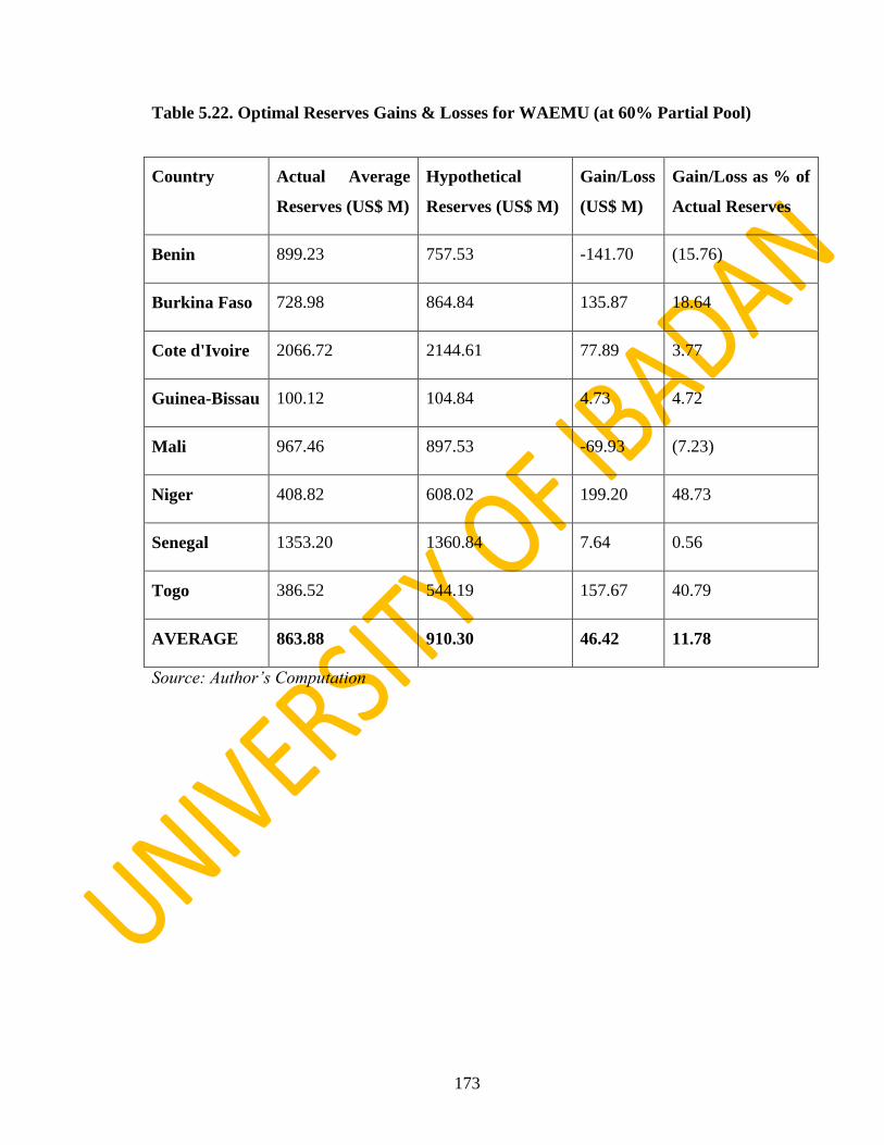
173
Table 5.22. Optimal Reserves Gains & Losses for WAEMU (at 60% Partial Pool)
Country Actual Average
Reserves (US$ M)
Hypothetical
Reserves (US$ M)
Gain/Loss
(US$ M)
Gain/Loss as % of
Actual Reserves
Benin 899.23 757.53 -141.70 (15.76)
Burkina Faso 728.98 864.84 135.87 18.64
Cote d'Ivoire 2066.72 2144.61 77.89 3.77
Guinea-Bissau 100.12 104.84 4.73 4.72
Mali 967.46 897.53 -69.93 (7.23)
Niger 408.82 608.02 199.20 48.73
Senegal 1353.20 1360.84 7.64 0.56
Togo 386.52 544.19 157.67 40.79
AVERAGE 863.88 910.30 46.42 11.78
Source: Author’s Computation

174
An analysis of “by how much gain/loss” here shows that Niger gains most from the
pooling amounting to 48% of it actual reserves followed by Togo and Burkina Faso.
Minimal positive gains are recorded by Cote d‟ Ivoire, Guinea Bissau and Senegal while
Benin and Mali have negative gains with Benin having the highest negative gain (table
5.22).
5.6.4 Evaluation of Reserves Pooling in the non-WAEMU Community
Table 5.23 shows the coverage indices without and with pooling for the non-WAEMU
countries. At the initial level of 0% pooling (without pooling), the coverage for the
countries show a wider divergence since each country is operating on its own. But as the
countries enter into a reserves pooling arrangement, the coverage indices for the different
countries begin to converge up till the case of complete pooling where all the coverage
indices are the same for all the countries.

175
Table 5.23. Coverage without and with Pooling for non-WAEMU Countries
Country 0% 10% 20% 30% 40% 50% 60% 70% 80% 90% 100%
C/Verde 1.74 1.77 1.77 1.77 1.86 1.86 1.86 1.86 1.86 1.86 1.86
Gambia 2.60 1.80 1.78 1.78 1.86 1.86 1.86 1.86 1.86 1.86 1.86
Ghana 1.97 1.90 1.85 1.82 1.89 1.89 1.88 1.87 1.87 1.86 1.86
Guinea 1.93 1.86 1.81 1.79 1.87 1.87 1.87 1.87 1.86 1.86 1.86
Liberia 0.76 1.75 1.76 1.76 1.85 1.86 1.86 1.86 1.86 1.86 1.86
Nigeria 1.72 1.73 1.73 1.74 1.83 1.84 1.84 1.85 1.85 1.85 1.86
S/Leone 1.60 1.79 1.78 1.77 1.86 1.86 1.86 1.86 1.86 1.86 1.86
Average 1.76 1.80 1.78 1.78 1.86 1.86 1.86 1.86 1.86 1.86 1.86
Source: Author’s Computation

176
For the non-WAEMU countries alone, the coverage indices appear to be lower than those
obtained for their WAEMU counterparts and even the ECOWAS region as a whole
discussed earlier. This is so since the reserves of most of the members here exhibit higher
variability as compared to that of the WAEMU community and also as compared to that
of ECOWAS, since their apparent vulnerabilities are more concealed by the presence of
other countries with lower variabilities. An average coverage of 1.86 appears to be the
optimal coverage for the non-WAEMU countries in the event of a reserve pooling
arrangement.
The gains and losses for the non-WAEMU as a community under different simulations of
pooling are shown in tables 5.24 and 5.25.
From table 5.25, it is observed that more individual countries will record negative gains
compared to their cases under the whole ECOWAS (Ghana and Guinea now have negative
gains under any pooling arrangement). This is not too far from expectations since the
analysis is more or less for a collection of countries with higher vulnerabilities and
exposure to shocks. That is, their vulnerabilities are exposed having being separated from
the countries in the WAEMU community. On the overall average, reserves pooling will
benefit the non-WAEMU countries taken as a unit should there be any reserves pooling
arrangement among them. Meanwhile, in the case of the non-WAEMU, the results show
that the pooling arrangement that yields the maximum possible gain is 70%. This actually
shows that since the coefficient of variation of reserves holding is higher here, more
reserves (a higher pooling arrangement) will be required to “cover” all the countries in the
community.

177
Table 5.24. Gains and Losses from Reserves Pooling for non-WAEMU
10% 20% 30% 40% 50% 60% 70% 80% 90% 100%
Cape Verde
Actual Average reserves (US$ M) 229.28 229.28 229.28 229.28 229.28 229.28 229.28 229.28 229.28 229.28
Coverage Index 1.77 1.77 1.77 1.86 1.86 1.86 1.86 1.85 1.85 1.85
Reserves Variability 131.85 131.85 131.85 131.85 131.85 131.85 131.85 131.85 131.85 131.85
Hypothetical Reserves (US$ M) 233.67 233.32 233.19 244.78 245.21 245.41 245.39 243.51 243.50 243.49
Gains/Losses (US$ Million) 4.40 4.05 3.92 15.50 15.93 16.13 16.11 14.23 14.22 14.21
Gambia
Actual Average reserves (US$ M) 126.00 126.00 126.00 126.00 126.00 126.00 126.00 126.00 126.00 126.00
Coverage Index 1.80 1.78 1.78 1.86 1.86 1.86 1.86 1.85 1.85 1.85
Reserves Variability 48.50 48.50 48.50 48.50 48.50 48.50 48.50 48.50 48.50 48.50
Hypothetical Reserves (US$ M) 87.44 86.49 86.16 90.30 90.37 90.39 90.34 89.62 89.59 89.56
Gains/Losses (US$ Million) -38.56 -39.51 -39.84 -35.70 -35.63 -35.61 -35.66 -36.39 -36.41 -36.44
Ghana
Actual Average reserves (US$ M) 1939.57 1939.57 1939.57 1939.57 1939.57 1939.57 1939.57 1939.57 1939.57 1939.57
Coverage Index 1.90 1.85 1.82 1.89 1.89 1.88 1.87 1.85 1.85 1.85
Reserves Variability 983.67 983.67 983.67 983.67 983.67 983.67 983.67 983.67 983.67 983.67
Hypothetical Reserves (US$ M) 1872.79 1817.94 1790.08 1862.22 1854.29 1847.93 1841.87 1823.24 1819.54 1816.53
Gains/Losses (US$ Million) -66.79 -121.64 -149.49 -77.35 -85.28 -91.65 -97.70 -116.34 -120.04 -123.05
Guinea
Actual Average reserves (US$ M) 108.12 108.12 108.12 108.12 108.12 108.12 108.12 108.12 108.12 108.12
Coverage Index 1.86 1.81 1.79 1.87 1.87 1.87 1.87 1.85 1.85 1.85
Reserves Variability 56.12 56.12 56.12 56.12 56.12 56.12 56.12 56.12 56.12 56.12
Hypothetical Reserves (US$ M) 104.62 101.56 100.56 105.07 104.95 104.84 104.70 103.79 103.70 103.64
Gains/Losses (US$ Million) -3.50 -6.56 -7.56 -3.06 -3.17 -3.28 -3.43 -4.33 -4.42 -4.49
Liberia
Actual Average reserves (US$ M) 86.66 86.66 86.66 86.66 86.66 86.66 86.66 86.66 86.66 86.66
Coverage Index 1.75 1.76 1.76 1.85 1.86 1.86 1.86 1.85 1.85 1.85
Reserves Variability 114.26 114.26 114.26 114.26 114.26 114.26 114.26 114.26 114.26 114.26
Hypothetical Reserves (US$ M) 199.57 200.93 201.36 211.64 212.17 212.45 212.51 210.94 210.97 211.00
Gains/Losses (US$ Million) 112.91 114.27 114.69 124.98 125.51 125.79 125.85 124.28 124.31 124.34
Nigeria
Actual Average reserves (US$ M) 29646.8 29646.85 29646.8 29646.8 29646.8 29646.8 29646.8 29646.8 29646.8 29646.85
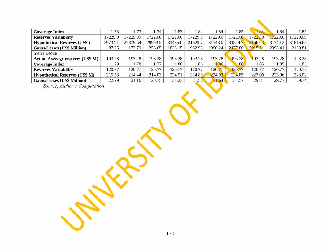
178
Coverage Index 1.73 1.73 1.74 1.83 1.84 1.84 1.85 1.84 1.84 1.85
Reserves Variability 17229.0 17229.09 17229.0 17229.0 17229.0 17229.0 17229.0 17229.0 17229.0 17229.09
Hypothetical Reserves (US$ ) 29734.1 29819.64 29903.5 31485.0 31629.7 31743.0 31824.7 31662.3 31740.2 31816.65
Gains/Losses (US$ Million) 87.25 172.79 256.65 1838.15 1982.93 2096.24 2177.86 2015.51 2093.41 2169.81
Sierra Leone
Actual Average reserves (US$ M) 193.28 193.28 193.28 193.28 193.28 193.28 193.28 193.28 193.28 193.28
Coverage Index 1.79 1.78 1.77 1.86 1.86 1.86 1.86 1.85 1.85 1.85
Reserves Variability 120.77 120.77 120.77 120.77 120.77 120.77 120.77 120.77 120.77 120.77
Hypothetical Reserves (US$ M) 215.58 214.44 214.03 224.51 224.80 224.92 224.85 223.09 223.06 223.02
Gains/Losses (US$ Million) 22.29 21.16 20.75 31.23 31.52 31.64 31.57 29.81 29.77 29.74
Source: Author’s Computation

179
Table 5.25. Summary of Gains/Losses from Reserves Pooling under different Degrees
of Pooling for non-WAEMU (US$ Million)
Country 10% 20% 30% 40% 50% 60% 70% 80% 90% 100%
C/ Verde 4.40 4.05 3.92 15.50 15.93 16.13 16.11 14.23 14.22 14.21
Gambia -38.56 -39.51 -39.84 -35.70 -35.63 -35.61 -35.66 -35.70 -35.98 -36.01
Ghana -66.79 -121.64 -149.49 -77.35 -85.28 -91.65 -97.70 -116.34 -120.04 -123.05
Guinea -3.50 -6.56 -7.56 -3.06 -3.17 -3.28 -3.43 -4.33 -4.42 -4.49
Liberia 112.91 114.27 114.69 124.98 125.51 125.79 125.85 124.28 124.31 124.34
Nigeria 87.25 172.79 256.65 1838.15 1982.93 2096.24 2177.86 2015.51 2093.41 2169.81
S/Leone 22.29 21.16 20.75 31.23 31.52 31.64 31.57 29.81 29.77 29.74
AVERAGE 16.86 20.65 28.44 270.54 290.26 305.61 316.37 289.64 300.18 310.65
Source: Author’s Computation

180
Table 5.26. Optimal Reserves Gains and Losses for non-WAEMU (at 70% Partial
Pool)
Country Actual
Average
Reserves
(US$ M)
Hypothetical
Reserves (US$
M)
Gain/Loss
(US$ M)
Gain/Loss as
% of Actual
Reserves
C/Verde 229.28 245.39 16.11 7.03
Gambia 126.00 90.34 -35.66 (28.30)
Ghana 1939.57 1841.87 -97.70 (5.04)
Guinea 108.12 104.70 -3.43 (3.17)
Liberia 86.66 212.51 125.85 145.22
Nigeria 29646.85 31824.71 2177.86 7.35
S/Leone 193.28 224.85 31.57 16.33
AVERAGE 4618.54 4934.91 316.37 19.92
Source: Author’s Computation

181
Considering the issue of how much gain for the non-WAEMU countries, it can be
observed from table 5.26 that Liberia has the highest positive gain from reserves pooling
among these countries. It has an overall gain of 145.22% of own reserves holding. This
positive gain is lower than its possible positive gain under an ECOWAS arrangement as a
whole which was recorded to be 205.48% of own reserves. This is due to evidence of a
higher risk factor in the arrangement here, though inside of ECOWAS, which does not
include countries of the WAEMU community. The country with the next highest positive
gain (though small when compared to Liberia) is Sierra Leone with 16.33% of actual
reserves while Nigeria and Cape Verde record minimal positive gains. However, the
remaining three countries (Gambia, Ghana and Guinea) will record negative gains from a
possible pooling arrangement with Gambia and Guinea having the highest and lowest
negative gains as percentages of their respective actual average international reserves
holdings.
The findings from this analysis corroborate those from other studies in other regions of the
world. Particularly, they support the findings of William, Polius and Hazel (2001) where
they present a comparison of the gains from reserves pooling between the Eastern
Caribbean Currency Union (ECCU) and the CFA Franc zone. Also, the findings here
agree with the study by Rajan, Siregar and Bird (2003) where they examined the gains to
be reaped if the East Asian economies were to pool their reserves together. In a related
study for the ASEAN (Association of South-Eastern Nations) plus three (APT) nations,
Rajan and Siregar (2004) find that the nations are better-off if they are to commit
themselves to a partial reserves pooling scheme than a complete pooling. They find that
50% pooling arrangement to be the optimal.

182
CHAPTER SIX
SUMMARY OF FINDINGS, CONCLUSION AND
RECOMMENDATION
6.1 Summary and Conclusion
This study examines reserves determinants and the effects of a prospective reserves
pooling on macroeconomic stability in the ECOWAS subregion. The study has
investigated the motivations, sources, and impact of the reserves accumulation, with a
focus on the impact on key macroeconomic variables. In the first instance, an analysis of
the supply and demand determinants of international reserves are evaluated for the region
through the panel data analysis where the fixed effects model and the random effects
models are estimated and examined.From the result of the fixed and random effect
models, it was observed that the results present sufficient evidence of the impact of the
included explanatory variables on the international reserves accumulation of the countries.
Also, through the robustness analysis, this study evaluated gains from a possible reserves
pooling in the ECOWAS region. The study finds that there are gains to be reaped for the
region as a whole if the countries therein decide to enter into an international reserves
pooling arrangement. By way of summary of the whole idea and benefits of reserves
pooling as evaluated in the study, consider the case of Liberia where within the period of
the analysis, its actual average reserves is US$86.66 million. Without belonging to the
pool, its coverage would be 0.76 given that its reserves variability is 114.26. However, by
belonging to the pool, its optimal coverage would become 2.32. Now if it would not be
part of the pool, and want to maintain this same level of coverage of 2.32, it means that
the country would have to hold reserves amounting to US$264.73 million (hypothetical
reserves). Hence, by actually holding only US$86.66 million in reserves, it has “saved”
itself the cost of having to accumulate extra reserves amounting to US$178.09 million
(which is the difference between 264.73 and 86.66) by belonging to the pool.
183
The spread of gains from possible reserves pooling for the region is not even. Some
countries will gain (more than others) while some others will lose (more than others) in a
reserves pooling scheme for the region. However, the countries with the gains constitute a
significantly larger proportion of the total countries thereby leading to overall average
gain for the entire region. At individual country level, Liberia will be the highest positive
gainer followed by Sierra Leone while Benin will be the highest negative gainer followed
by Mali.
For the region as a whole, a partial reserves pooling arrangement where members
contribute only a percentage of own reserve to the pool is found to be most desirable
rather than a complete pooling arrangement. The percentage contribution that maximizes
gains from reserves pooling for the ECOWAS region as a whole is found to be 60%. This
percentage is also found to be the optimal for the WAEMU community while 70% is
found to be the optimal for the non-WAEMU community.
The two monetary communities in the ECOWAS (WAEMU and non-WAEMU) would
benefit differently from a collective international reserves pooling arrangement. WAEMU
countries would benefit less in a reserves pooling arrangement compared to its non-
WAEMU counterparts should the region as a whole decides to enter into a reserves
pooling arrangement. This is largely due to the fact that the WAEMU countries have been
together for long and have actually attained a higher level of macroeconomic stability and
less international reserves variability.
The response of macroeconomic variables to shock or innovations from unpooled and
pooled reserves are also considered in the study using the impulse response function and
variance decomposition of the VAR framework. The study finds robust evidence of
possible macroeconomic stability from reserves pooling as the estimation reveals that a
46.71% stability can be attained in the region‟s macroeconomy under a reserves pooling
arrangement relative to when the countries in the region operate in their
individual/autonomous state. This becomes even more significant for the countries of the
region when considering the fact that it is a 60% partial pool that the study finds to be
optimal for the entire region. This implies that about 40% of resources can be freed up for

184
other developmental purposes in each of the individual countries apart from having
unrestricted access to a larger pool of reserves from the central union.
It should be noted that in any form of monetary integration, countries will not gain equally
at the same time. Some will gain at one time or area but will lose in another time or area.
It should also be seen like that in the case of a reserves pooling arrangement since reserves
pooling is suppose to be a phase of a much wider monetary integration and optimal
currency establishment and the very rationale for belonging to a monetary union is for a
country to provide benefits to other countries who are part of the union and in need at one
time with the understanding that they will do same for the country at some other times
when in need as well. There are possibilities that the gains estimated here may not be so
obvious under some other circumstances such as lack of trust among members,
misappropriation and misuse of the reserves pool as well as the fear of extravagance and
profligacy of some members.
6.2 Policy Recommendations
This study is on international reserves pooling and macroeconomic stability in ECOWAS.
There is increasing consensus within the region that intra-regional macroeconomic
stability is a desirable policy objective. Several options for bringing about such stability,
including the adoption of a common currency in the long run and implementation of
exchange rate mechanism are being proposed. However, for all these options to be
effective in bringing about the desired stability of the regional currency, a necessary
impetus in this regard is the pooling of international reserves. One of the key reasons for
pooling reserves in the region is to facilitate stability of the regional currency when finally
in operation.
Since pooled reserves are held to prevent the exchange rates of member countries from
deviating significantly from perceived central rates under the exchange rate mechanism,
reserve pooling arrangement must be followed with a framework for exchange rate
coordination at the regional level to achieve the above objective. This means that the
capacity of the monetary authority in the region to supervise and effectively intervene in
the foreign exchange market depends on the quantum of pooled reserves. Besides, a

185
reserve pooling initiative will only be meaningful if fragmented foreign exchange markets
in the region are effectively harmonised to facilitate smooth intervention in the single
foreign exchange market that will emerge when the single currency is eventually
introduced. Hence, in addition to the framework for pooling reserves, there must be a
framework for harmonising fragmented foreign exchange market in the region.
The study finds and recommends partial reserves pooling arrangement for the region
which allows for some flexibility in the sense that each country contributes an amount that
offers them the highest benefits to the pool. International reserves pooling is a fragment of
the subject matter of monetary integration. The countries in the region have been handed
some convergence criteria in which reserves adequacy is one of the criteria.
Thus, the ECOWAS countries should intensify macroeconomic reforms in order to meet
up with the convergence criteria in order to reap the gains from the macroeconomic
stability examined from reserves pooling in this study as well as for the smooth take off of
a single currency operation.
6.3 Limitations of the Study
This study has largely focused on the empirical examination of reserves pooling and
macroeconomic stability in ECOWAS. However, the institutional bureaucracy and the
political economy of pooling have not been captured. Thus, the results and estimated gains
from pooling and the impact of pooling on macroeconomic stability may be altered when
some of these factors are accounted for.
Only some selected key macroeconomic variables (as identified by the OCA as the
sources of macroeconomic shocks) are employed for the estimation of the macroeconomic
stability in the region. Thus, possibilities abound that there can be a change in result if
more (or different sets of) macroeconomic variables are employed.
A research of this magnitude is challenging and tasking especially in the area of monetary
integration and OCAs as well as when dealing with a panel of countries and having a
macroeconomic outlook. Thus, study drawbacks associated with imprecision in the
sourcing and use of secondary data as well as other unobservable inconsistencies,

186
inadequacies and inaccuracies in the expressions, presentations and interpretations of facts
in the course of the study are also acknowledged as possible snags and shortcomings.
187
REFERENCES
Abeng, M. O. 2007. Foreign Exchange Reserves Accumulation: Implications for the
Nigerian Economy. The Bullion Vol. 31, No 3, Central Bank of Nigeria.
Abdel-Salam, O. H. 1970. The Evolution of African Monetary Institutions The Journal
of Modern African Studies. Vol. 8, No. 3., Oct., pp. 339-362.
Aizenman, J. and J. Lee 2006. International Reserves: Precautionary Versus
Mercantilist Views: Theory and Evidence. NBER Working Paper No. 11366.
Aizenman, J., Y. Lee, and Y. Rhee 2004. International Reserves Management and Capital
Mobility: Policy Considerations and a Case Study of Korea. NBER Working Paper
No. 10534.
Aizenman, J. and N. Marion 2002. The High Demand for International Reserves in the Far
East: What‟s Going On? Journal of the Japanese and International Economies
17(3): 370–400.
Aizenman, J. and N. Marion 2004. International Reserve Holding with Sovereign
Risk and Costly Tax Collection.The Economic Journal, 114 (July), pp. 569-91.
Aizenman, J. 2007. Large Hoarding of International Reserves and the Emerging Global
Economic Architecture Paper Prepared for Growth and Business Cycles in Theory
and Practice Conference, University Of Manchester 12th -13th July 2007.
Alberola E., Buisan A., and S. Fernandez de Lis 2003. The Quest for Nominal and Real
Convergence through Integration in Europe and Latin America. In Regional
Integration in Europe and Latin American Monetary and Financial Aspects
England: Ashgate Publishing Limited.
Araujo, A. and M. Leon 2004. Speculative Attacks on Debts and Optimum Currency
Area: A Welfare Analysis. Bank of Brazil Working Paper Series. 84.
Arellano, M. and O. Bover 1995. Another Look at the Instrumental Variable Estimation of
Error-Components Models.Journal of Econometrics Vol. 68 (Jul., 1995), 29-51.
Athanasoulis, S. G. and E. van Wincoop 2000. Growth uncertainty and risk sharing.

188
Journal of Monetary Economics 45(3), 477–505.
Attanasio, O. Barr A. Cardenas,J.Genicot G. andMeghir C. 2011. Risk Pooling, Risk
Preferences, and Social Networks. Review of Economics and Statistics Vol. 82, pp.
182–211.
Barnichon R. 2008 “International Reserves and Self-Insurance against External Shocks”
IMF Working Paper WP/08/149 (Washington: International Monetary Fund).
Bastourre D. Carrera J., and Ibarlucia J. 2006. Why Countries Accumulate Foreign
Reserves? A Dynamic Panel Approach.
www.aaep.org.ar/anales/works/works2006/Bastourre_Carrera_Ibarlucia.pdf
Basu, S., Bi, R., and Kannan, P. 2010. Regional Reserve Pooling Arrangements CEPR
Discussion Paper No 6085.
Bayoumi, T. and B. Eichengreen 1992. Shocking Aspect of European Monetary
Unification National Bureau of Economic Research Working Paper No. 3949.
Bayoumi , T. and T. Ostry 1997. Macroeconomic Shocks and Trade Flows within Sub-
Sahara Africa: Implication for Optimum Currency Arrangement. Journal Of
African Economics October Vol. 6 No 3 pp.412-44.
Ben-Bassat, A. and D. Gottlieb 1992. Optimal International Reserves and Sovereign Risk.
Journal of International Economics vol. 33, PP 354-62.
Blanchard, O.J. and D. Quah 1989. The Dynamic Effect of Aggregate Demand and
Supply Disturbances.The American Review, Vol.79, No.4, pp.655-673.
Bilson, J.F.O., and J.A. Frenkel, 1979. Dynamic Adjustment and the Demand for
International Reserves. NBER Working Paper No. 403.
Bold, S. and Dercon, S. 2009. Group-Based Funeral Insurance in Ethiopia and
Tanzania.World Development, 34(4), 685-703.
Boughton J.M, 1991. The CFA Zone, Currency Union and Monetary Standard.
Washington: IMF Working Paper No WP/91/133, 1991.
Buchanan, J. 1965. An Economic Theory of Clubs.EconomicaVol. 32, pp. 1-14.

189
Busch G.K. 2009.The Economic and Political Effects of the CFA Zone.
http://saoti.overblog.com/article-17347736.html
Callen, M., J. Imbs, and P. Mauro 2011.Pooling Risk among Countries.CEPR
Discussion Paper No 6461.
Coase R. H. 1960.The Problem of Social Cost.Journal of Law and Economics.Vol 3
pp 1-44
Choi C. and S. Baek 2004. “Exchange Rate Regimes and International Reserves”
http://www.eusanz.org/pdf/conf04/choi_baek.pdf.
Choi, W.G., S. Sharma, and M. Strömqvist 2007. “Capital Flows, Financial Integration,
and International Reserve Holdings: The Recent Experience of Emerging Markets
and Advanced Economies” IMF Working Paper WP/07/151.
Cole, H. L., and M. Obstfeld 1991. Commodity Trade and International Risk sharing:
how much do financial markets matter? Journal of Monetary Economics 28(3), 3–
24.
Collins R., and J. M. Burns 2007.A history of Sub-Saharan Africa. Cambridge
University Press
Club Bruxelles, 1996.The West African Economic and Monetary Union, Springboard for
Economic Development in West Africa. Bruxelles.
Debrun, X., P. Masson and C. Pattillo 2005.Monetary Union in West Africa: Who might
lose, and why? Canadian Journal of Economics Vol. 38, No.2 pp. 454-481.
Devarajan, S. and J. De Melo 1987. Evaluating Participation in African Monetary Unions:
A Statistical Analysis of the CFA Zones. World Development, 15, 483-96.
Devarajan, S and M. Walton 1994. Preserving the CFA Zone Macroeconomic
Coordination after Devaluation. World Bank Policy Research Working Paper 1316
DeGrauwe, P. 2000. Economics of Monetary Union. Oxford University Press: Oxford,
UK.

190
De Weerdt, J. and Dercon, S. 2006. Risk-Sharing Networks and Insurance Against
Illness. Journal of Development Economics, 81(2), 337-356.
Dodsworth, J.R., 1975. Reserve Pooling an Application of the Theory of Clubs.
EconomiaInternazionale, Vol. 44, pp. 209-22.
Dramani L. A. 2010. Convergence and Economic integration in Africa: a Case of the
Franc Zone countries. African Economic Research Consortium (AERC) Research
Paper 200
Drummond P. and A. Dhasmana 2008.Foreign Reserve Adequacy in Sub-Saharan
Africa.IMF Working Paper WP/08/150 (International Monetary Fund).
Ebi, E. 2002.Rgeional Currency Areas: Lessons from the West African Sub-region and
Nigeria‟s Policy Stance.A paper Prepared for meeting of senior Officials of
Central Banks. September 2002.
ECB, European Central Bank 2006. The Accumulation of Foreign Reserves.
Occasional Paper No. 43 (February).
Edison, H. 2003. Are Foreign Exchange Reserves in Asia Too High? IMF World
Economic Outlook September 2003.
Egwaikhide, F. O. 1999.Determinants of Imports in Nigeria: A Dynamic Specification.
African Economic Research Consortium (AERC) Research Paper 91, Nairobi.
Eichengreen, B. and T. Bayoumi 1992. Is Asia an Optimum Currency Area? Can It
Become One? Regional, Global and Historical Perspectives on Asian Monetary
Relations. In S. Collignon, J. Pisani-Ferry, and Y.C. Park eds. Exchange Rate
Policies in Emerging Asian Countries, 347-366. London Routledge.
Elhiraika, A. and L. Ndikumana 2007. Reserves Accumulation in African Countries:
Sources, Motivations, and Effects.A paper Submitted to African Economic
Conference: Opportunities and Challenges for Africain the Global Arena, by ADB
and ECA, AddisAbaba, Ethiopia, 15-17 November 2007.
Erkel-Rousse, H. and J. Melitz. 1995. New Empirical Evidence on the Costs Of
European Monetary Union. .INSEE Working Paper No. 9516.

191
Fafchamps, M. and F. Gubert 2007.The formation of risk sharing networks.Journal of
Development Economics 83(2), 326-350.
Fajana, O. 2011.Framework for Harmonizing Foreign Exchange Markets and Pooling
of Reserves by West African Central Bank (WACB).A Paper Prepared for
the West African Monetary Institute (WAMI), June, 2011
Flood, R. and N.P. Marion 2002. Holding International Reserves in an Era of High Capital
Mobility. Brookings Trade Forum 2001, Washington D.C.: The Brookings
Institution, 1-68.
Floyd, J. E. 2005. Vector Autoregression Analysis: Estimation and Interpretation.
Available at http://www.economics.utoronto.ca/jfloyd/papers/varnote.ps.
Frenkel, J. A. and B. Jovanovic 1981. Optimal International Reserves: A Stochastic
Framework. Economic Journal, 91, 507-514.
Frenkel, J. 1978. International Reserves: Pegged Exchange rates and Managed
Float.Carnegie- Rochester Conference Series 9, 111-140.
Frankel, J. A and A.K. Rose 1998. The Endogeneity of the Optimum Currency Area
Criteria.The Economic Journal 108(449), 1009-1025.
Friedman 1953. Essay in Positive Economics. Chicago: University of Chicago.
Gosselin M. and N. Parent 2005.An Empirical Analysis of Foreign Exchange Reserves in
Emerging Asia.Bank of Canada Working Paper No 38 (Bank of Canada Ottawa,
Ontario, Canada).
Greenspan, A. 1999.Currency Reserves and Debt. Remarks by Chairman Alan Greenspan
before the World Bank Conference on Recent Trends in Reserve Management,
Washington, 29 April.
Hashimoto Y. 2008 “Too Much For Self-Insurance? Asian Foreign Reserves” Hkimr
Working Paper No.6 Http://Ssrn.Com/Abstract=1160483
Heller, H.R. 1966.Optimal International Reserves.Economic Journal 76(302): 296–311.

192
Heller, R.H. and M.S. Khan. 1978. The Demand for International Reserves Under Fixed
and Floating Exchange Rates. IMF Staff Papers 25(4): 623–49.
Hogendorn, J. S. and Gemery, H. A. 1988. Continuity in West African Monetary
History?An Outline of Monetary Development.African Economic History.17: 127-
146.
Hopkins, A. G. 1973.An Economic History of West Africa. Longman, London.
Horvath, J. and R. Grabowski 1997. Prospects of African integration in light of the
theory of optimum currency areas.Journal of Economic Integration. Vol12
No.1, 1–25.
Horvath R. and L. Komarek, 2002 Optimum Currency Area Theory: An Approach
For Thinking About Monetary Integration Warwick Economic Research Papers
No 647.
Imbs, J. and P. Mauro 2007.Pooling Risk Among Countries. IMF Working Paper 07/132,
International Monetary Fund.
IMF 2003. Balance of Payment Manual.International Monetary Fund, Fifth Edition.
IMF 2007. IMF Country Reports.Selected Issues and Statistical Appendix No. 07/126
(Washington, March).
IMF 2008 International Financial Statistics (IFS).An International Monetary Fund
Publication.
Ingram, J.C. 1973. The Case for the European Monetary Integration Princeton
University, Essays in International Finance. No. 98.
Iyoha, M. A. 2003.A Common Monetary Policies for the West African Monetary Zone:
Rationale and Design. West African Financial And Economic Review, Vol.1, No.1.
Jeanne, O. 2007.International Reserves in Emerging Market Countries: Too Much of a
Good Thing? Brooking Papers on Economic Activity 1: 2007.
Jeanne, O., and R Rancière 2006. The Optimal Level of International Reserves for
Emerging Market Countries: Formulas and Applications. IMF Working Paper
WP/06/229, Washington: International Monetary Fund.
193
Jerome, A. 2005.Reflections on the Economic Community of West African States
(ECOWAS) at Thirty and the Challenges of Economic Integration in West Africa
in Ogun, et al. ed. New World Press, Ibadan.
Johansen, Soren. 1995. Likelihood-Based Inference in Cointegrated Vector
Autoregressive Models. Oxford: Oxford University Press.
Kenen , P. B. 1969. The Theory of Optimum Currency Area: An Eclectic View. In R. A.
Mundell and A. Swoboda. Eds.,Monetary Problems and International Economy.
Chicago: University of Chicago Press, pp.41-60.
Kronberger, R. 2004.A Cost- Benefit Analysis of a Monetary Union for MERCOSUR
with Particular Emphasis on the Optimum Currency Area Theory.Economic
Working Paper Archive. EWPA/0407/0407010.
Kydland, F. E., and E. C. Prescott 1977 “Rules Rather than Discretion: the Inconsistency
of Optimal Plans” Journal of Political Economy, 85(3), 473-492.
Lane, P.R. and D. Burke 2001.The Empirics of Foreign reserves.Open Economies Review,
12(4), 423– 34.
Lin M. and J. Wang 2005 “Foreign Exchange Reserves and Inflation: an Empirical Study
of Five East Asian Economies”
http://pubfin.nccu.edu.tw/faculty/wang/search1/for5.pdf
Masson, P. and C. Pattillo 2001.Monetary Union in West Africa (ECOWAS) - Is it
desirable and how could it be achieved? IMF Ocassion Paper No.204,Washington,
DC.
Masson, P. and C.Pattillo 2004.A Single Currency for Africa. International Monetary
Fund (IMF) Finance And Development, Pp. 9-15.
Mazzeo, Dominico 1984.African Regional Organisations(Cambridge: Cambridge
University Press).
McCarthy, C. 2003.The Southern African Customs Union in Transition.African
affairs102: 605-630.

194
McKinnon, R. 1963.Optimum Currency Areas.American Economic Review, Vol. 53,
No. 4, 717-25.
Medhora, R. 1992.The Gain from Reserve Pooling in the West African Monetary
Union.EconomiaInternazionale, 45, pp.209-22.
Mendoza, R.U. 2004. International Reserve-Holding in the Developing World: Self
Insurance in a Crisis-Prone Era?Emerging Markets Review 5(1): 61–82.
Mongeli F. P. 2010. On the Benefits and Costs of a Monetary Union. Centre for
Economic Policy Research (CEPR), Policy Insight, No. 46.
Mundell, R. A. 1961.A Theory of Optimal Currency Areas.American Economic Review,
51, 657-665.
Murgai, R., P. Winters, E. Sadoulet and A. de Janvry 2002.Localized and Incomplete
MutualInsurance.Journal of Development Economics 67, 245-274.
Nda, M. 2006. Effective Reserves Management in Nigeria: Issues, Challenges and
Prospects. The Bullion Vol. 30, No. 3, Central Bank of Nigeria.
Ng, Y. 1975.The Economic Theory of Clubs: Pareto Optimality
Conditions.Economica,Vol. 32, pp. 291-98.
Nindi , A. G. 2011. The Implication of Monetary Integration within the SADC Region for
Regional Economic Integration and Development.PHD Thesis, Department of
Economics and History, Rhodes University.
Nnanna, O. J, E.A Essien, E.A Onwioduokit and E.T Adamgbe 2007.Empirical Evidence
of the Benefits of Economic and Monetary Integration in the West African
Monetary Zone.West African Journal of Monetary and Economic Integration,
Vol.7, No.2. Accra, Ghana.
Obaseki, P.J. 2007. Sources, Currency Composition and the Uses of External
Reserves.The Bullion Vol. 31, No. 2, Central Bank of Nigeria.
Obstfeld, M. 1994.Risk-Taking, Global Diversification, and Growth.American Economic
Review,84(5), 1310–29.

195
Ogunkola E. O. 2005.An Evaluation of The Viability Of A Single Monetary Zone In
ECOWAS.African Economic Research Consortium (AERC) Research Paper 147.
Ogunkola E. O. and A. Jerome 2005.The Second Monetary Zone in West Africa and the
Future of a Single Monetary Zone in Sub-Saharan Africa.West African Journal of
Economics and Monetary Integration, Vol. 5 No.1.
Okafor, H. O 2011.Analysis of the Cost and Benefit of a Common Currency for the
Second West African Monetary Zone (WAMZ).An Unpublished Ph.D Thesis at
the Department of Economics, University of Ibadan.
Okorie, G. 2007.External Reserves Management in Nigeria.The Bullion Vol. 31, No. 2,
Central Bank of Nigeria.
Olawoyin, G. A. 2007. Risk Management in the Investment of External Reserves in
Nigeria.The Bullion Vol. 31, No. 2, Central Bank of Nigeria.
Oyejide, T. A. 2012. Costs and Benefits of Monetary Union: A Pedagogical Note.African
Journal of Economic Policy.Vol. 19 No. 1.
Pedroni, P. 1999. Purchasing Power Parity Tests in Cointegrated Panels.Working paper,
Department of Economics, Indiana University.
Radelet, S., and J. Sachs. 1998. The East Asian Financial Crisis: Diagnosis,
Remedies, Prospects. Brookings Paper of Economic Activity 1, pp.1-90.
Rajan, R., R. Siregar, and G. Bird. 2003. Examining the Case of Reserves Pooling in East
Asia: Empirical Analysis. Discussion Paper no. 219, University of Adelaide.
Rajan, R., and R. Siregar 2004.Centralized Reserve Pooling For the ASEAN Plus Three
(APT) Countries.Monetary And Financial Cooperation In East Asia. United
Kingdom: Macmillan Press For The Asian Development Bank.
Rassekh, F. 1998. The Convergence Hypothesis, Theory and Evidence. Open Economics
Review 9: 85-105.
Reinhart C. M. and K. S. Rogoff 2004. The Modern History of Exchange Rate
Arrangements: A Reinterpretation. Quarterly Journal of Economics, 119(1), 1-48.

196
Ricci, A. L. 2008. A Model of an Optimum Currency Area. International Monetary Fund
Research Department
Rodrik, D. 2006.The Social Cost of Foreign Exchange Reserves.Paper Presented at the
American Economic Association Meetings, January.
Ruiz-Arranz M. and M. Zavadjil 2008.Are Emerging Asia‟s Reserves Really Too
High?IMF Working Paper WP/08/192. ( International Monetary Fund).
Satyanath S. and A. Subramanian 2004. What Determines Long-Run Macroeconomic
Stability? Democratic Institutions. IMF Working Paper, November. 2004
Sen, H. 1999. The IMF and World Bank Approaches to Macroeconomic Management in
Developing Countries. available at:
http://akson.sgh.waw.pl/~cwojcik/teaching/if_spring2005/imf%20world%20bank
%20approach%20to%20macroeconomic%20management.pdf. Accessed June 13,
2011.
Shamsuddeen, U. 2005. Towards a More Strategic Management of Nigeria‟s Foreign
Reserves.A Paper Presentation at the Annual Conference of the Nigerian
Economic Society at Sheraton Hotels and Towers Lagos, August 2005.
Sims, C. 1980. Macroeconomics and Reality.Econometrica, 48, pp.1-49.
Soludo, C. C. 2007 “Preserving Stability and Accelerating Growth” A Paper Presentation
at the 3rd
Economist Conference Business Roundtable with the Government of
Nigeria, Abuja.
Tarawalie A. B. 2012. Analyzing Fiscal Sustainability in the West African Monetary
Zone (WAMZ). A Paper Presented at the African Economic Research
Consortiums (AERC) Bi-Annual June 2012.
Tesar, L. L. 1995. Evaluating the Gains from International Risk sharing. Carnegie-
Rochester Conference Series on Public Policy, 42, 95–143.
Van Wincoop, E. 1994. Welfare gains from international risk sharing. Journal of
Monetary Economics, 34(2), 175–200.
197
---------- 1999. How big are potential welfare gains from international risk sharing?
Journal of International Economics, 47(1), 109–135.
WAMI 2008. Single Currency or the ECOWAS: Options and Prospects. Working Paper
No.12/08, Accra, Ghana.
Vaubel, R. 1978. Real Exchange Rate Changes in the European Community: A New
Approach to the Determination of Optimum Currency Areas. Journal Of
International Economics, Vol.8,Pp.319-339.
Williams, M. V. 2005. Foreign Exchange Reserves: How Much Is Enough? A
Presentation at the Twentieth Adlith Brown Memorial Lecture. Central Bank of
Bahamas, November 2005.
Williams, O., T. Pollius and S. Hazel 2001. Reserve Pooling in the Eastern Caribbean
Currency Union and the CFA Franc Zone: A Comparative Analysis.IMF Working
Paper No.01/104.
Zafar, and K. Kubota 2003.Regional Integration in Central Africa, Key Issues.African
Regional Working Paper No 52, 2003.

198
199
Appendices
Appendix 1: Variance Decomposition Period S.E. RESU RESP GOVT
1 3.416419 0.002209 1.073715 98.92408
2 4.483322 0.064259 0.753941 99.18180
3 5.184239 0.089669 0.613827 99.29650
4 5.700588 0.108542 0.597911 99.29355
5 6.117079 0.117514 0.708091 99.17439
6 6.479011 0.120737 0.944759 98.93450
7 6.810316 0.120357 1.302879 98.57676
8 7.123112 0.118050 1.768328 98.11362
9 7.422802 0.114946 2.322937 97.56212
10 7.711114 0.111818 2.946665 96.94152
11 7.987907 0.109178 3.619491 96.27133
12 8.252242 0.107347 4.322558 95.57010
13 8.502976 0.106500 5.038900 94.85460
14 8.739091 0.106709 5.753842 94.13945
15 8.959835 0.107965 6.455159 93.43688
16 9.164777 0.110204 7.133064 92.75673
17 9.353799 0.113325 7.780065 92.10661
18 9.527062 0.117206 8.390753 91.49204
19 9.684964 0.121713 8.961543 90.91674
20 9.828085 0.126710 9.490402 90.38289
Cholesky Ordering:
RESU RESP GOVT
Period S.E. RESU RESP INV
1 3.441448 0.222292 0.021413 99.75629
2 4.401919 0.669539 0.545055 98.78541
3 5.098841 1.049923 1.091443 97.85863
4 5.628685 1.522233 1.705664 96.77210
5 6.071036 2.035573 2.364919 95.59951
6 6.464962 2.571502 3.093105 94.33539
7 6.832021 3.105657 3.906413 92.98793
8 7.182977 3.618541 4.815629 91.56583
9 7.522454 4.094717 5.824330 90.08095
10 7.851639 4.523263 6.929591 88.54715
11 8.169958 4.897471 8.122874 86.97966
12 8.476075 5.214375 9.391219 85.39441
13 8.768476 5.474122 10.71856 83.80732
14 9.045786 5.679282 12.08704 82.23368
15 9.306924 5.834165 13.47823 80.68760
16 9.551159 5.944191 14.87416 79.18165
17 9.778108 6.015352 16.25812 77.72653
18 9.987710 6.053778 17.61523 76.33100
19 10.18018 6.065405 18.93275 75.00184
20 10.35596 6.055758 20.20029 73.74396
Cholesky Ordering:
RESU RESP INV

200
Period S.E. RESU RESP GDPGR
1 4.136784 0.129039 3.390503 96.48046
2 5.064019 1.844231 3.766920 94.38885
3 5.742970 1.812414 4.147563 94.04002
4 6.230369 1.847893 4.509066 93.64304
5 6.598553 1.988710 4.753746 93.25754
6 6.887145 2.137960 4.935014 92.92703
7 7.119717 2.268366 5.088015 92.64362
8 7.311985 2.369935 5.229124 92.40094
9 7.474366 2.444662 5.365062 92.19028
10 7.613981 2.497775 5.497504 92.00472
11 7.735760 2.534493 5.626082 91.83942
12 7.843170 2.559171 5.749754 91.69108
13 7.938689 2.575175 5.867456 91.55737
14 8.024124 2.585038 5.978337 91.43662
15 8.100827 2.590635 6.081832 91.32753
16 8.169835 2.593335 6.177637 91.22903
17 8.231972 2.594133 6.265676 91.14019
18 8.287918 2.593739 6.346052 91.06021
19 8.338248 2.592652 6.419000 90.98835
20 8.383464 2.591218 6.484855 90.92393
Cholesky Ordering:
RESU RESP GDPGR
Period S.E. RESU RESP TRF
1 3.468498 0.218589 10.29725 89.48416
2 4.493375 0.146395 12.31906 87.53455
3 5.197585 0.110594 14.18622 85.70319
4 5.729724 0.098503 15.92666 83.97483
5 6.164943 0.097211 17.56446 82.33833
6 6.545176 0.103523 19.11201 80.78447
7 6.892745 0.114850 20.57346 79.31169
8 7.219778 0.129678 21.94964 77.92068
9 7.532367 0.146860 23.24019 76.61294
10 7.833189 0.165530 24.44475 75.38972
11 8.123025 0.185003 25.56350 74.25150
12 8.401695 0.204743 26.59740 73.19786
13 8.668603 0.224324 27.54823 72.22744
14 8.923055 0.243421 28.41852 71.33806
15 9.164438 0.261785 29.21142 70.52679
16 9.392300 0.279237 29.93062 69.79014
17 9.606382 0.295652 30.58020 69.12415
18 9.806619 0.310955 31.16448 68.52457
19 9.993121 0.325105 31.68794 67.98696
20 10.16615 0.338096 32.15513 67.50678
Cholesky Ordering:
RESU RESP TRF

201
Period S.E. RESU RESP DEBT
1 4.122319 5.302020 8.832203 85.86578
2 5.030360 3.025707 5.590737 91.38356
3 5.673536 1.996024 3.953021 94.05095
4 6.120923 1.461139 3.102729 95.43613
5 6.461813 1.385614 2.636973 95.97741
6 6.735600 1.746803 2.365994 95.88720
7 6.965121 2.471695 2.197809 95.33050
8 7.163197 3.447546 2.087352 94.46510
9 7.337397 4.551529 2.013634 93.43484
10 7.492413 5.676901 1.968650 92.35445
11 7.631353 6.746328 1.951184 91.30249
12 7.756424 7.713259 1.962933 90.32381
13 7.869290 8.556375 2.006027 89.43760
14 7.971264 9.271941 2.081608 88.64645
15 8.063425 9.866852 2.189197 87.94395
16 8.146684 10.35344 2.326640 87.31992
17 8.221833 10.74603 2.490378 86.76359
18 8.289568 11.05896 2.675883 86.26516
19 8.350517 11.30546 2.878125 85.81642
20 8.405251 11.49726 3.091974 85.41077
Cholesky Ordering:
RESU RESP DEBT
Period S.E. RESU RESP EXR
1 4.140258 0.127301 0.056324 99.81637
2 5.067806 0.734617 0.182476 99.08291
3 5.740355 1.392231 0.337019 98.27075
4 6.210287 2.221122 0.408664 97.37021
5 6.563338 3.174439 0.426120 96.39944
6 6.837919 4.208911 0.419038 95.37205
7 7.058609 5.284042 0.403792 94.31217
8 7.240867 6.367767 0.388014 93.24422
9 7.394882 7.435996 0.375026 92.18898
10 7.527493 8.471497 0.366282 91.16222
11 7.643373 9.462507 0.362515 90.17498
12 7.745769 10.40149 0.364210 89.23430
13 7.836982 11.28408 0.371774 88.34414
14 7.918675 12.10831 0.385567 87.50612
15 7.992091 12.87389 0.405897 86.72021
16 8.058185 13.58178 0.432992 85.98523
17 8.117719 14.23380 0.466982 85.29922
18 8.171326 14.83234 0.507888 84.65977
19 8.219549 15.38016 0.555618 84.06422
20 8.262865 15.88023 0.609971 83.50980
Cholesky Ordering:
RESU RESP EXR
202
Appendix 2: Reverse Ordering of Variance Decomposition Government Spending
Variance Decomposition of
GOVT:
Period S.E. GOVT RESP RESU 1 2.754833 100.0000 0.000000 0.000000
2 3.288216 99.62396 0.236124 0.139921
3 3.719594 99.55018 0.263060 0.186758
4 4.014826 99.56049 0.232938 0.206572
5 4.236776 99.57382 0.221631 0.204549
6 4.405569 99.52467 0.280972 0.194361
7 4.537210 99.38343 0.433101 0.183469
8 4.641740 99.14219 0.681413 0.176394
9 4.726232 98.80582 1.018675 0.175507
10 4.795660 98.38631 1.431885 0.181808
11 4.853602 97.89915 1.905442 0.195409
12 4.902653 97.36103 2.423116 0.215854
13 4.944711 96.78834 2.969312 0.242348
14 4.981176 96.19626 3.529835 0.273905
15 5.013085 95.59822 4.092316 0.309467
16 5.041218 95.00563 4.646390 0.347979
17 5.066161 94.42784 5.183711 0.388445
18 5.088366 93.87220 5.697845 0.429958
19 5.108187 93.34418 6.184096 0.471722
20 5.125906 92.84765 6.639292 0.513060
Cholesky Ordering: GOVT RESP RESU
Investment
Variance Decomposition
of INV:
Period S.E. INV RESP RESU 1 4.251007 100.0000 0.000000 0.000000
2 5.252084 99.13514 0.786879 0.077985
3 5.993790 98.28497 1.551078 0.163953
4 6.520795 97.28321 2.402437 0.314350
5 6.919538 96.18879 3.308345 0.502869
6 7.229828 94.99211 4.293876 0.714015
7 7.478494 93.69919 5.371719 0.929090
8 7.683309 92.31854 6.548166 1.133293
9 7.856625 90.86285 7.821346 1.315802
10 8.007154 89.34737 9.182669 1.469956
11 8.141087 87.78901 10.61825 1.592739
12 8.262811 86.20538 12.11054 1.684086
13 8.375405 84.61403 13.63986 1.746108
14 8.480988 83.03174 15.18590 1.782361
15 8.580973 81.47390 16.72891 1.797191
16 8.676263 79.95416 18.25062 1.795218
17 8.767397 78.48410 19.73496 1.780938
18 8.854657 77.07319 21.16835 1.758458
19 8.938159 75.72872 22.53994 1.731335

203
20 9.017913 74.45598 23.84151 1.702506 Cholesky Ordering: INV
RESP RESU
GDP growth
Variance Decomposition of
GDPGR:
Period S.E. GDPGR RESP RESU 1 7.359799 100.0000 0.000000 0.000000
2 7.755973 96.72184 0.914491 2.363670
3 7.858900 95.87922 1.810839 2.309946
4 7.886851 95.34972 2.355550 2.294734
5 7.903896 94.93945 2.723004 2.337548
6 7.917958 94.61610 2.987081 2.396823
7 7.930336 94.34913 3.200939 2.449934
8 7.941164 94.12495 3.387457 2.487597
9 7.950691 93.93280 3.556701 2.510501
10 7.959156 93.76510 3.712568 2.522329
11 7.966748 93.61677 3.856426 2.526801
12 7.973598 93.48439 3.988749 2.526864
13 7.979802 93.36558 4.109810 2.524610
14 7.985427 93.25864 4.219930 2.521434
15 7.990527 93.16224 4.319545 2.518219
16 7.995146 93.07532 4.409195 2.515482
17 7.999322 92.99701 4.489500 2.513492
18 8.003090 92.92653 4.561124 2.512351
19 8.006482 92.86319 4.624753 2.512052
20 8.009527 92.80640 4.681073 2.512527
Cholesky Ordering: GDPGR RESP RESU
Variance Decomposition of
TRF:
Period S.E. TRF RESP RESU 1 10.87175 100.0000 0.000000 0.000000
2 13.37009 99.63909 0.194837 0.166070
3 15.42544 99.21666 0.513780 0.269556
4 16.94922 98.67190 0.929429 0.398670
5 18.15976 98.05532 1.413755 0.530924
6 19.13532 97.38239 1.950022 0.667588
7 19.93476 96.67099 2.523337 0.805676
8 20.59701 95.93576 3.120902 0.943338
9 21.15040 95.18982 3.731381 1.078802
10 21.61596 94.44450 4.344900 1.210597
11 22.00980 93.70948 4.953005 1.337516
12 22.34446 92.99277 5.548612 1.458616

204
13 22.62991 92.30086 6.125942 1.573201
14 22.87415 91.63878 6.680425 1.680793
15 23.08368 91.01030 7.208593 1.781112
16 23.26384 90.41800 7.707959 1.874043
17 23.41902 89.86349 8.176901 1.959613
18 23.55289 89.34750 8.614542 2.037962
19 23.66855 88.87005 9.020633 2.109321
20 23.76856 88.43056 9.395448 2.173992 Cholesky Ordering: TRF
RESP RESU
External Debt
Variance Decomposition of
DEBT:
Period S.E. DEBT RESP RESU 1 46.21528 100.0000 0.000000 0.000000
2 78.87002 98.63430 1.062453 0.303249
3 103.5684 96.90388 2.430201 0.665920
4 121.0652 95.03962 3.673627 1.286749
5 133.0145 93.10835 4.691702 2.199952
6 141.0715 91.12684 5.496553 3.376606
7 146.5551 89.14028 6.130667 4.729050
8 150.3919 87.21557 6.640090 6.144339
9 153.1808 85.41876 7.064977 7.516260
10 155.2895 83.79694 7.436898 8.766165
11 156.9390 82.37203 7.778838 9.849136
12 158.2641 81.14402 8.106242 10.74973
13 159.3506 80.09827 8.428385 11.47334
14 160.2560 79.21277 8.749764 12.03746
15 161.0217 78.46359 9.071396 12.46501
16 161.6779 77.82819 9.391969 12.77984
17 162.2474 77.28692 9.708807 13.00427
18 162.7476 76.82349 10.01864 13.15787
19 163.1913 76.42470 10.31816 13.25714
20 163.5884 76.08004 10.60441 13.31555
Cholesky Ordering: DEBT RESP RESU
Exchange rate
Variance Decomposition of
EXR:
Period S.E. EXR RESP RESU 1 0.259451 100.0000 0.000000 0.000000
2 0.390048 99.35934 0.496730 0.143930
3 0.486375 98.65687 0.945438 0.397690
4 0.563318 97.90306 1.259799 0.837144
5 0.627637 97.08994 1.475473 1.434585
6 0.683028 96.21725 1.634320 2.148430
7 0.731700 95.30196 1.763894 2.934146

205
8 0.775070 94.36546 1.880735 3.753803
9 0.814098 93.42767 1.994555 4.577780
10 0.849464 92.50464 2.111040 5.384319
11 0.881677 91.60827 2.233487 6.158240
12 0.911125 90.74671 2.363728 6.889557
13 0.938120 89.92508 2.502659 7.572262
14 0.962919 89.14614 2.650556 8.203302
15 0.985738 88.41095 2.807267 8.781787
16 1.006762 87.71929 2.972344 9.308364
17 1.026151 87.07013 3.145125 9.784746
18 1.044048 86.46184 3.324801 10.21336
19 1.060580 85.89248 3.510462 10.59706
20 1.075861 85.35989 3.701141 10.93897
Cholesky Ordering: EXR RESP RESU
Appendix 3: VAR Estimates
Vector Autoregression Estimates
Date: 07/04/13 Time: 02:09
Sample (adjusted): 1983 2011
Included observations: 381 after adjustments
Standard errors in ( ) & t-statistics in [ ]
RESU RESP GOVT
RESU(-1) 0.841850 -2.283015 0.036658
(0.05286) (0.59176) (0.04263)
[ 15.9252] [-3.85803] [ 0.85999]
RESU(-2) 0.028771 1.874955 -0.035013
(0.05274) (0.59042) (0.04253)
[ 0.54549] [ 3.17565] [-0.82327]
RESP(-1) 0.002027 1.345220 -0.004819
(0.00437) (0.04891) (0.00352)
[ 0.46380] [ 27.5016] [-1.36767]
RESP(-2) 0.005485 -0.357888 0.006302
(0.00459) (0.05134) (0.00370)
[ 1.19585] [-6.97036] [ 1.70386]
GOVT(-1) -0.091888 -0.707886 0.654549
(0.06129) (0.68607) (0.04942)
[-1.49927] [-1.03180] [ 13.2447]
GOVT(-2) 0.056181 0.218915 0.205154
(0.05921) (0.66283) (0.04775)
[ 0.94880] [ 0.33027] [ 4.29677]
C 1.562761 16.46011 1.612440
(0.50312) (5.63205) (0.40569)

206
[ 3.10612] [ 2.92258] [ 3.97453]
R-squared 0.816077 0.939845 0.759751
Adj. R-squared 0.813127 0.938880 0.755897
Sum sq. resids 4365.298 547014.6 2838.324
S.E. equation 3.416419 38.24403 2.754833
F-statistic 276.5772 973.8791 197.1196
Log likelihood -1005.177 -1925.442 -923.1719
Akaike AIC 5.313265 10.14405 4.882792
Schwarz SC 5.385705 10.21649 4.955232
Mean dependent 10.57914 103.5308 13.00886
S.D. dependent 7.903100 154.6934 5.575814
Determinant resid covariance (dof adj.) 123691.8
Determinant resid covariance 116998.7
Log likelihood -3844.966
Akaike information criterion 20.29379
Schwarz criterion 20.51110
Vector Autoregression Estimates
Date: 07/04/13 Time: 02:29
Sample (adjusted): 1983 2011
Included observations: 379 after adjustments
Standard errors in ( ) & t-statistics in [ ]
RESU RESP INV
RESU(-1) 0.795591 -2.491916 0.043544
(0.05385) (0.60815) (0.06652)
[ 14.7747] [-4.09752] [ 0.65465]
RESU(-2) 0.090889 2.101820 0.019571
(0.05417) (0.61181) (0.06692)
[ 1.67777] [ 3.43540] [ 0.29247]
RESP(-1) 0.001001 1.333505 0.011217
(0.00424) (0.04783) (0.00523)
[ 0.23625] [ 27.8805] [ 2.14427]
RESP(-2) 0.007081 -0.347212 -0.009033
(0.00446) (0.05041) (0.00551)
[ 1.58633] [-6.88769] [-1.63838]
INV(-1) -0.007525 0.588004 0.715251
(0.04177) (0.47179) (0.05160)
[-0.18014] [ 1.24632] [ 13.8610]
INV(-2) -0.020644 -0.655988 0.144426
(0.04086) (0.46151) (0.05048)
[-0.50520] [-1.42141] [ 2.86126]
C 1.442962 11.43604 1.657812
(0.40771) (4.60460) (0.50362)
[ 3.53918] [ 2.48361] [ 3.29179]

207
R-squared 0.823121 0.938152 0.790996
Adj. R-squared 0.820268 0.937155 0.787625
Sum sq. resids 4405.806 561958.8 6722.435
S.E. equation 3.441448 38.86698 4.251007
F-statistic 288.5222 940.4631 234.6448
Log likelihood -1002.648 -1921.440 -1082.717
Akaike AIC 5.327959 10.17646 5.750486
Schwarz SC 5.400684 10.24919 5.823211
Mean dependent 10.82759 107.4864 18.07861
S.D. dependent 8.117620 155.0403 9.224438
Determinant resid covariance (dof adj.) 309701.6
Determinant resid covariance 292856.3
Log likelihood -3998.652
Akaike information criterion 21.21189
Schwarz criterion 21.43006
Vector Autoregression Estimates
Date: 07/04/13 Time: 03:49
Sample (adjusted): 1983 2011
Included observations: 417 after adjustments
Standard errors in ( ) & t-statistics in [ ]
RESU RESP GDPGR
RESU(-1) 0.689510 -3.309965 -0.299536
(0.05036) (0.55015) (0.08960)
[ 13.6916] [-6.01648] [-3.34317]
RESU(-2) 0.159496 2.735041 0.357403
(0.05078) (0.55470) (0.09034)
[ 3.14114] [ 4.93068] [ 3.95633]
RESP(-1) 0.005100 1.296384 0.024230
(0.00429) (0.04683) (0.00763)
[ 1.18954] [ 27.6810] [ 3.17685]
RESP(-2) -0.000682 -0.316190 -0.019591
(0.00444) (0.04846) (0.00789)
[-0.15378] [-6.52414] [-2.48217]
GDPGR(-1) 0.008813 -0.239662 0.294076
(0.02706) (0.29556) (0.04813)
[ 0.32572] [-0.81087] [ 6.10948]
GDPGR(-2) -0.025243 -0.684460 0.079781
(0.02658) (0.29036) (0.04729)
[-0.94972] [-2.35727] [ 1.68714]
C 1.579289 16.35527 1.323191
(0.34619) (3.78193) (0.61592)

208
[ 4.56186] [ 4.32458] [ 2.14832]
R-squared 0.753088 0.933486 0.161374
Adj. R-squared 0.749474 0.932513 0.149101
Sum sq. resids 7016.322 837333.4 22208.32
S.E. equation 4.136784 45.19156 7.359799
F-statistic 208.4180 959.0266 13.14912
Log likelihood -1180.274 -2177.317 -1420.513
Akaike AIC 5.694358 10.47634 6.846586
Schwarz SC 5.762060 10.54404 6.914288
Mean dependent 10.83581 121.1477 3.709593
S.D. dependent 8.264882 173.9593 7.978605
Determinant resid covariance (dof adj.) 1691826.
Determinant resid covariance 1608048.
Log likelihood -4754.668
Akaike information criterion 22.90488
Schwarz criterion 23.10799
Vector Autoregression Estimates
Date: 07/04/13 Time: 03:53
Sample (adjusted): 1983 2011
Included observations: 393 after adjustments
Standard errors in ( ) & t-statistics in [ ]
RESU RESP TRF
RESU(-1) 0.814820 -2.263197 -0.160300
(0.05249) (0.58223) (0.16453)
[ 15.5231] [-3.88712] [-0.97429]
RESU(-2) 0.063287 1.927850 0.112311
(0.05220) (0.57898) (0.16361)
[ 1.21244] [ 3.32974] [ 0.68645]
RESP(-1) 0.000238 1.304175 0.019171
(0.00436) (0.04838) (0.01367)
[ 0.05461] [ 26.9547] [ 1.40217]
RESP(-2) 0.006440 -0.314609 -0.009366
(0.00454) (0.05036) (0.01423)
[ 1.41833] [-6.24672] [-0.65808]
TRF(-1) 0.026642 0.314623 0.692429
(0.01657) (0.18382) (0.05194)
[ 1.60764] [ 1.71160] [ 13.3302]
TRF(-2) -0.016136 -0.389432 0.188578
(0.01635) (0.18137) (0.05125)
[-0.98686] [-2.14722] [ 3.67949]
C 0.447792 14.09196 7.804050
(0.52171) (5.78678) (1.63526)

209
[ 0.85832] [ 2.43520] [ 4.77237]
R-squared 0.828634 0.937989 0.800700
Adj. R-squared 0.825970 0.937025 0.797602
Sum sq. resids 4643.765 571331.9 45623.28
S.E. equation 3.468498 38.47252 10.87175
F-statistic 311.0809 973.1094 258.4632
Log likelihood -1042.894 -1988.539 -1491.875
Akaike AIC 5.342972 10.15542 7.627864
Schwarz SC 5.413752 10.22620 7.698645
Mean dependent 10.87620 106.1924 65.19313
S.D. dependent 8.314371 153.3081 24.16555
Determinant resid covariance (dof adj.) 1809236.
Determinant resid covariance 1714271.
Log likelihood -4493.587
Akaike information criterion 22.97500
Schwarz criterion 23.18734
Vector Autoregression Estimates
Date: 07/04/13 Time: 03:57
Sample (adjusted): 1983 2011
Included observations: 417 after adjustments
Standard errors in ( ) & t-statistics in [ ]
RESU RESP DEBT
RESU(-1) 0.673659 -3.405268 -1.111389
(0.05106) (0.55906) (0.57241)
[ 13.1941] [-6.09111] [-1.94161]
RESU(-2) 0.159414 3.012443 -0.069982
(0.05122) (0.56084) (0.57423)
[ 3.11232] [ 5.37133] [-0.12187]
RESP(-1) 0.006668 1.277353 -0.168504
(0.00437) (0.04786) (0.04901)
[ 1.52550] [ 26.6873] [-3.43838]
RESP(-2) -0.000974 -0.310871 0.176569
(0.00448) (0.04903) (0.05020)
[-0.21752] [-6.34070] [ 3.51740]
DEBT(-1) 0.000422 0.095695 1.448987
(0.00367) (0.04014) (0.04110)
[ 0.11504] [ 2.38403] [ 35.2562]
DEBT(-2) -0.002680 -0.066903 -0.533375
(0.00369) (0.04041) (0.04137)
[-0.72610] [-1.65571] [-12.8920]
C 1.831045 9.561227 20.39552
(0.37053) (4.05715) (4.15404)
[ 4.94165] [ 2.35663] [ 4.90980]
210
R-squared 0.754811 0.933646 0.942651
Adj. R-squared 0.751223 0.932675 0.941811
Sum sq. resids 6967.340 835326.1 875699.4
S.E. equation 4.122319 45.13736 46.21528
F-statistic 210.3636 961.4954 1123.194
Log likelihood -1178.813 -2176.817 -2186.658
Akaike AIC 5.687353 10.47394 10.52114
Schwarz SC 5.755054 10.54164 10.58884
Mean dependent 10.83581 121.1477 121.8307
S.D. dependent 8.264882 173.9593 191.5872
Determinant resid covariance (dof adj.) 58282124
Determinant resid covariance 55396047
Log likelihood -5492.651
Akaike information criterion 26.44437
Schwarz criterion 26.64747
Vector Autoregression Estimates
Date: 07/04/13 Time: 04:00
Sample (adjusted): 1983 2011
Included observations: 417 after adjustments
Standard errors in ( ) & t-statistics in [ ]
RESU RESP EXR
RESU(-1) 0.687580 -3.395320 -0.003721
(0.05037) (0.55319) (0.00316)
[ 13.6495] [-6.13774] [-1.17867]
RESU(-2) 0.159682 2.701788 -0.001784
(0.05099) (0.55990) (0.00320)
[ 3.13193] [ 4.82548] [-0.55833]
RESP(-1) 0.005351 1.311214 -0.000511
(0.00425) (0.04670) (0.00027)
[ 1.25821] [ 28.0757] [-1.91844]
RESP(-2) -0.000997 -0.335290 0.000584
(0.00437) (0.04804) (0.00027)
[-0.22790] [-6.97875] [ 2.12858]
EXR(-1) 0.075344 -14.95729 1.115118
(0.76001) (8.34613) (0.04763)
[ 0.09914] [-1.79212] [ 23.4139]
EXR(-2) -0.039838 14.62926 -0.147977
(0.73776) (8.10184) (0.04623)
[-0.05400] [ 1.80567] [-3.20074]
C 1.379524 17.79721 0.280983
(0.50809) (5.57962) (0.03184)
[ 2.71513] [ 3.18968] [ 8.82499]
R-squared 0.752673 0.932674 0.990366
Adj. R-squared 0.749053 0.931689 0.990225

211
Sum sq. resids 7028.113 847561.6 27.59903
S.E. equation 4.140258 45.46673 0.259451
F-statistic 207.9537 946.6287 7024.336
Log likelihood -1180.624 -2179.849 -25.55618
Akaike AIC 5.696038 10.48848 0.156145
Schwarz SC 5.763739 10.55618 0.223846
Mean dependent 10.83581 121.1477 4.776690
S.D. dependent 8.264882 173.9593 2.624151
Determinant resid covariance (dof adj.) 2200.697
Determinant resid covariance 2091.721
Log likelihood -3369.229
Akaike information criterion 16.26009
Schwarz criterion 16.46320
Appendix 4: Unit Roots Test
Panel unit root test: Summary
Series: GDPGR
Date: 07/03/13 Time: 01:05
Sample: 1981 2011
Exogenous variables: Individual effects
User-specified lags: 1
Newey-West automatic bandwidth selection and Bartlett kernel
Cross-
Method Statistic Prob.** sections Obs
Null: Unit root (assumes common unit root process)
Levin, Lin & Chu t* -6.55820 0.0000 15 429
Null: Unit root (assumes individual unit root process)
Im, Pesaran and Shin W-stat -9.78706 0.0000 15 429
ADF - Fisher Chi-square 153.915 0.0000 15 429
PP - Fisher Chi-square 267.794 0.0000 15 444
** Probabilities for Fisher tests are computed using an asymptotic Chi
-square distribution. All other tests assume asymptotic normality.
Panel unit root test: Summary
Series: D(GOVT)
Date: 07/04/13 Time: 17:07
Sample: 1981 2011
Exogenous variables: Individual effects
User-specified lags: 1
Newey-West automatic bandwidth selection and Bartlett kernel
Cross-
Method Statistic Prob.** sections Obs
Null: Unit root (assumes common unit root process)
Levin, Lin & Chu t* -11.0824 0.0000 15 374
Null: Unit root (assumes individual unit root process)
Im, Pesaran and Shin W-stat -12.1192 0.0000 15 374

212
ADF - Fisher Chi-square 191.731 0.0000 15 374
PP - Fisher Chi-square 327.888 0.0000 15 391
** Probabilities for Fisher tests are computed using an asymptotic Chi
-square distribution. All other tests assume asymptotic normality.
Panel unit root test: Summary
Series: D(INV)
Date: 07/04/13 Time: 17:10
Sample: 1981 2011
Exogenous variables: Individual effects
User-specified lags: 1
Newey-West automatic bandwidth selection and Bartlett kernel
Cross-
Method Statistic Prob.** sections Obs
Null: Unit root (assumes common unit root process)
Levin, Lin & Chu t* -6.39935 0.0000 15 374
Null: Unit root (assumes individual unit root process)
Im, Pesaran and Shin W-stat -10.2697 0.0000 15 374
ADF - Fisher Chi-square 166.948 0.0000 15 374
PP - Fisher Chi-square 317.868 0.0000 15 389
** Probabilities for Fisher tests are computed using an asymptotic Chi
-square distribution. All other tests assume asymptotic normality.
Panel unit root test: Summary
Series: D(EXR)
Date: 07/04/13 Time: 17:15
Sample: 1981 2011
Exogenous variables: Individual effects
User-specified lags: 1
Newey-West automatic bandwidth selection and Bartlett kernel
Balanced observations for each test
Cross-
Method Statistic Prob.** sections Obs
Null: Unit root (assumes common unit root process)
Levin, Lin & Chu t* -6.50336 0.0000 15 420
Null: Unit root (assumes individual unit root process)
Im, Pesaran and Shin W-stat -8.53900 0.0000 15 420
ADF - Fisher Chi-square 129.701 0.0000 15 420
PP - Fisher Chi-square 194.325 0.0000 15 435
** Probabilities for Fisher tests are computed using an asymptotic Chi
-square distribution. All other tests assume asymptotic normality.
Panel unit root test: Summary
Series: D(DEBT)
Date: 07/03/13 Time: 01:04
Sample: 1981 2011

213
Exogenous variables: Individual effects
User-specified lags: 1
Newey-West automatic bandwidth selection and Bartlett kernel
Cross-
Method Statistic Prob.** sections Obs
Null: Unit root (assumes common unit root process)
Levin, Lin & Chu t* -7.27960 0.0000 15 415
Null: Unit root (assumes individual unit root process)
Im, Pesaran and Shin W-stat -8.47671 0.0000 15 415
ADF - Fisher Chi-square 128.122 0.0000 15 415
PP - Fisher Chi-square 240.414 0.0000 15 430
** Probabilities for Fisher tests are computed using an asymptotic Chi
-square distribution. All other tests assume asymptotic normality.
Panel unit root test: Summary
Series: D(RESP)
Date: 07/03/13 Time: 01:11
Sample: 1981 2011
Exogenous variables: Individual effects
User-specified lags: 1
Newey-West automatic bandwidth selection and Bartlett kernel
Cross-
Method Statistic Prob.** sections Obs
Null: Unit root (assumes common unit root process)
Levin, Lin & Chu t* -10.6370 0.0000 15 415
Null: Unit root (assumes individual unit root process)
Im, Pesaran and Shin W-stat -10.3981 0.0000 15 415
ADF - Fisher Chi-square 161.489 0.0000 15 415
PP - Fisher Chi-square 209.493 0.0000 15 430
** Probabilities for Fisher tests are computed using an asymptotic Chi
-square distribution. All other tests assume asymptotic normality.
Panel unit root test: Summary
Series: D(RESU)
Date: 07/03/13 Time: 01:12
Sample: 1981 2011
Exogenous variables: Individual effects
User-specified lags: 1
Newey-West automatic bandwidth selection and Bartlett kernel
Cross-
Method Statistic Prob.** sections Obs
Null: Unit root (assumes common unit root process)
Levin, Lin & Chu t* -8.59180 0.0000 15 401
Null: Unit root (assumes individual unit root process)
Im, Pesaran and Shin W-stat -10.5852 0.0000 15 401
ADF - Fisher Chi-square 165.102 0.0000 15 401
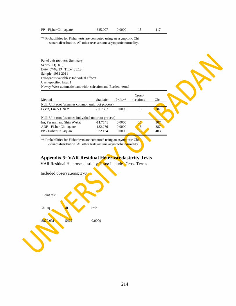
214
PP - Fisher Chi-square 345.007 0.0000 15 417
** Probabilities for Fisher tests are computed using an asymptotic Chi
-square distribution. All other tests assume asymptotic normality.
Panel unit root test: Summary
Series: D(TRF)
Date: 07/03/13 Time: 01:13
Sample: 1981 2011
Exogenous variables: Individual effects
User-specified lags: 1
Newey-West automatic bandwidth selection and Bartlett kernel
Cross-
Method Statistic Prob.** sections Obs
Null: Unit root (assumes common unit root process)
Levin, Lin & Chu t* -9.67387 0.0000 15 387
Null: Unit root (assumes individual unit root process)
Im, Pesaran and Shin W-stat -11.7141 0.0000 15 387
ADF - Fisher Chi-square 182.276 0.0000 15 387
PP - Fisher Chi-square 322.134 0.0000 15 403
** Probabilities for Fisher tests are computed using an asymptotic Chi
-square distribution. All other tests assume asymptotic normality.
Appendix 5: VAR Residual Heteroscedasticity Tests
VAR Residual Heteroscedasticity Tests: Includes Cross Terms
Included observations: 370
Joint test:
Chi-sq df Prob.
8870.031 5472 0.0000