international trade — — | | 13: firm-level trade empirics (ii) · lecture 13: firm-level trade...

— —

14.581

Spring 2013

14.581 International Trade Lecture 13: Firm-Level Trade Empirics (II)

14.581 Firm-Level Trade Empirics (II)

— —

Plan for Today’s Lecture on Firm-Level Trade

1

2

Trade flows: intensive and extensive margins

Exporting across to multiple destinations

14.581 Firm-Level Trade Empirics (II) Spring 2013 2 / 46

Intensive and Extensive Margins in Trade Flows

With access to micro data on trade flows at the firm-level, a key question to ask is whether trade flows expand over time (or look bigger in the cross-section) along the:

Intensive margin: the same firms (or product-firms) from country i export more volume (and/or charge higher prices—we can also decompose the intensive margin into these two margins) to country j . Extensive margin: new firms (or product-firms) from country i are penetrating the market in country j .

This is really just a decomposition—we can and should expect trade to expand along both margins.

Recently some papers have been able to look at this. A rough lesson from these exercises is that the extensive margin seems more important (in a purely ‘accounting’ sense, not necessarily a causal sense).


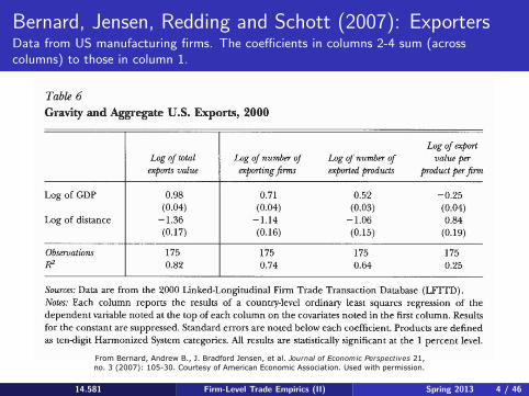
Bernard, Jensen, Redding and Schott (2007): ExportersData from US manufacturing firms. The coefficients in columns 2-4 sum (acrosscolumns) to those in column 1.

Andrew B. Bernard, J. Bradford Jensen, StephenJ. Redding, and Peter K. Schott 123

suppressed. as ten-digit Harmonized System categories. All results are statistically signift at the 1 percent level.


Data are from the 2000 Linked-Longitudinal Firm Trade Transaction Database (LFTTD). Each column reports the results of a country-level ordinary least squares regression of the

variable noted at the top of each column on the covariates noted in the first column. Results constant are suppressed. Standard errors are noted below each coefficient. Products are defined

Harmonized System categories. All results are statistically significant at the 1 percent level.

and Exporting The empirical literature on firms in international trade has been concerned

From Bernard, Andrew B., J. Bradford Jensen, et al. Journal of Economic Perspectives 21,no. 3 (2007): 105-30. Courtesy of American Economic Association. Used with permission.

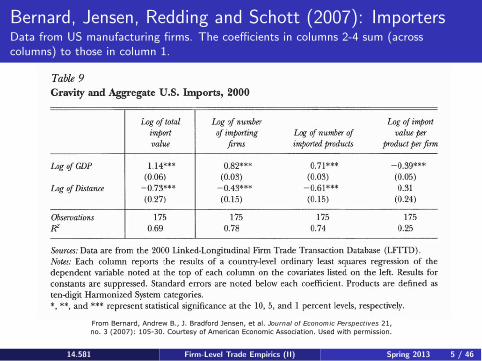
Bernard, Jensen, Redding and Schott (2007): ImportersData from US manufacturing firms. The coefficients in columns 2-4 sum (acrosscolumns) to those in column 1.


From Bernard, Andrew B., J. Bradford Jensen, et al. Journal of Economic Perspectives 21,no. 3 (2007): 105-30. Courtesy of American Economic Association. Used with permission.

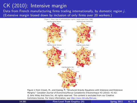
CK (2010): Intensive margin Data from French manufacturing firms trading internationally, by domestic region j . (Extensive margin biased down by inclusion of only firms over 20 workers.)

Figure 1: Mean value of individual-firm exports (single-region firms, 1992)

0.02

0.46

0.75

1.32

3.45

32.61

Importing country: Belgium

0.00

0.10

0.25

0.56

2.32

25.57

0.00

0.58

1,23

2.18

7.60

37.01

0,00

0,18

0,39

0,68

1,60

4,03

0,22

0,51

0,88

2,48

8,96

Importing country: Switzerland

Importing country: SpainImporting country: Germany

Importing country: Italy

Belgium

Germany

Switzerland

Italy

Spain

Belgium

Germany

Switzerland

Italy

Spain

Belgium

Germany

Switzerland

Italy

Spain

Belgium

Germany

Switzerland

Italy

Spain

Belgium

Germany

Switzerland

Italy

Spain

24


Figure 1 from Crozet, M., and Koenig, P. "Structural Gravity Equations with Intensive and ExtensiveMargins." Canadian Journal of Economics/Revue Canadienne D'économique 43 (2010): 41-62.© John Wiley And Sons Inc. All rights reserved. This content is excluded from our CreativeCommons license. For more information, see http://ocw.mit.edu/fairuse.

http://ocw.mit.edu/fairuse

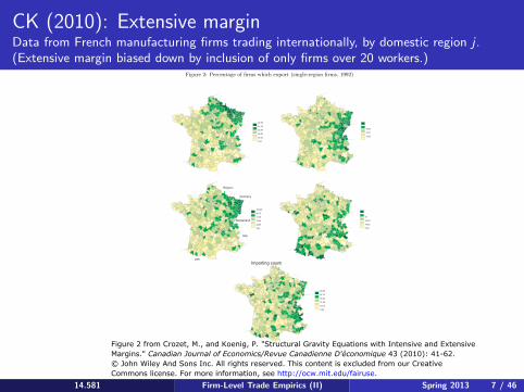
CK (2010): Extensive margin Data from French manufacturing firms trading internationally, by domestic region j . (Extensive margin biased down by inclusion of only firms over 20 workers.)

Figure 2: Percentage of firms which export (single-region firms, 1992)

9.37

26.92

38.00

46.87

61.53

92.59

16.66

23.71

34.21

60.00

92.85

5.00

22.85

32.05

41.93

68.75

100.00

0.00

18.42

25.00

31.1

1

41.66

80.00

6.66

18.18

25.00

33.33

46.15

80.00

0.00

Importing country: Belgium Importing country: Switzerland

Importing country: SpainImporting country: Germany

Importing country: Italy

Belgium

Germany

Switzerland

Italy

Spain

Belgium

Germany

Switzerland

Italy

Spain

Belgium

Germany

Switzerland

Italy

Spain

Belgium

Germany

Switzerland

Italy

Spain

Belgium

Germany

Switzerland

Italy

Spain

25


Figure 2 from Crozet, M., and Koenig, P. "Structural Gravity Equations with Intensive and ExtensiveMargins." Canadian Journal of Economics/Revue Canadienne D'économique 43 (2010): 41-62.© John Wiley And Sons Inc. All rights reserved. This content is excluded from our CreativeCommons license. For more information, see http://ocw.mit.edu/fairuse.


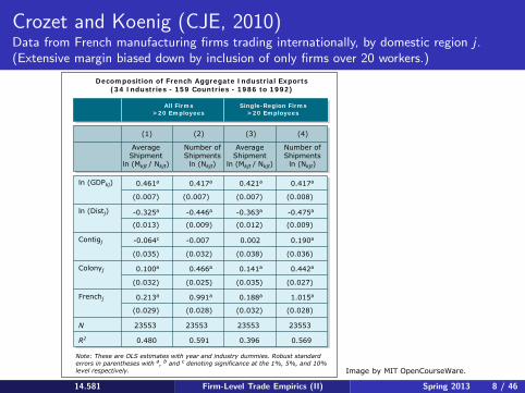
Crozet and Koenig (CJE, 2010) Data from French manufacturing firms trading internationally, by domestic region j . (Extensive margin biased down by inclusion of only firms over 20 workers.)


ln (GDPkj)

ln (Distj)

Contigj

Colonyj

Frenchj

0.461a 0.417a 0.421a 0.417a

-0.475a

0.190a

0.442a0.141a0.466a0.100a

0.213a 0.991a 0.188a 1.015a

-0.363a-0.446a-0.325a

-0.064c

(0.007)

(0.013) (0.012)

(0.036)(0.038)

(0.035)

(0.028)(0.032)(0.028)(0.029)

(0.027)

(0.032)

(0.032)

(0.035)

(0.025)

(0.007)

(0.009) (0.009)

(0.007) (0.008)

-0.007 0.002

N

R2

23553 23553 23553 23553

0.480 0.591 0.396 0.569

AverageShipment

ln (Mkjt / Nkjt)

Number ofShipments

ln (Nkjt)

AverageShipment

ln (Mkjt / Nkjt)

Number ofShipments

ln (Nkjt)

(1) (2) (3) (4)

All Firms>20 Employees

Single-Region Firms>20 Employees

Decomposition of French Aggregate Industrial Exports(34 Industries - 159 Countries - 1986 to 1992)

Note: These are OLS estimates with year and industry dummies. Robust standarderrors in parentheses with a, b and c denoting significance at the 1%, 5%, and 10%level respectively. Image by MIT OpenCourseWare.

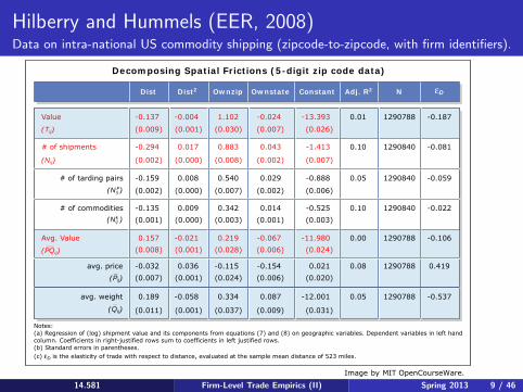
Hilberry and Hummels (EER, 2008) Data on intra-national US commodity shipping (zipcode-to-zipcode, with firm identifiers).


-0.888

-0.525

0.029

0.014

0.540

0.342

0.008

0.009

-0.159

-0.135

(0.002)

(0.001)

(0.007)

(0.011)

(0.001)

(0.001)

(0.024)

(0.037)

(0.006)

(0.009)

(0.020)

(0.031)

(0.000)

(0.000)

(0.007)

(0.003)

(0.002)

(0.001)

(0.006)

(0.003)

1290840

1290788

1290840

1290840

1290788

1290788

1290788

-0.059

-0.022

-0.106

0.419

-0.537

-0.081

-0.187

0.10

0.01

0.05

0.10

0.00

0.080.021-0.154-0.1150.036

0.334 0.087 -12.001-0.0580.189

-0.032

0.05

Notes:(a) Regression of (log) shipment value and its components from equations (7) and (8) on geographic variables. Dependent variables in left handcolumn. Coefficients in right-justified rows sum to coefficients in left justified rows.(b) Standard errors in parentheses.(c) εD is the elasticity of trade with respect to distance, evaluated at the sample mean distance of 523 miles.

Dist Ownzip Ownstate ConstantDist2 Adj. R2 N εD

# of tarding pairs(Nij )F

# of commodities(Nij )k

avg. price(Pij)

_

avg. weight

(Qij)_

Decomposing Spatial Frictions (5-digit zip code data)

-0.294

(0.002) (0.000) (0.008) (0.002) (0.007)

(0.026)(0.007)(0.030)(0.001)(0.009)

-1.413

-11.980-0.0670.219-0.021(0.008)0.157

(0.001) (0.028) (0.006) (0.024)

0.0430.8830.017

-0.137 -0.004 1.102 -0.024 -13.393Value

(Tij)

# of shipments

(Nij)

Avg. Value

(PQij)__

Image by MIT OpenCourseWare.

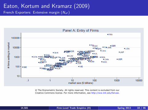
Eaton, Kortum and Kramarz (2009) French Exporters: Extensive margin (NnF )


© The Econometric Society. All rights reserved. This content is excluded from ourCreative Commons license. For more information, see http://ocw.mit.edu/fairuse.


DENGRE NORFIN SWIAUTROMNIA SOUARGSYR THASIN TAIAUL14.581 Firm-Level Trade Empirics (II) Spring 2013 11 / 46

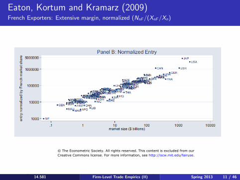
Eaton, Kortum and Kramarz (2009)French Exporters: Extensive margin, normalized (NnF/(XnF/Xn)



FRA

BELNET

GERITA UNK

IREDENGREPOR

SPANOR

SWEFIN SWIAUT

YUGTUR

USRGEE

CZEHUNROM

BUL

ALB

MOR

ALG

TUN

LIYEGY

SUDMAUMAL BUKNIG

CHASEN

SIE

LIB COTGHATOGBEN

NIA

CAM

CEN

ZAI

RWABUR

ANGETH

SOM

KENUGA TAN

MOZMAD MAS

ZAMZIM

MAWSOU

USA

CANMEX

GUAHONELS

NIC

COSPAN

CUB

DOM

JAMTRI

COLVEN

ECUPER

BRA

CHI

BOL

PARURU

ARGSYR

IRQIRN

ISRJOR

SAU

KUWOMA

AFG PAKIND

BANSRINEP

THAVIE

INO

MAYSINPHI

CHN

KOR JAPTAIHOK

AUL

PAP NZE

.001

.01

.1

1

10

perc

entil

es (2

5, 5

0, 7

5, 9

5) b

y m

arke

t ($

milli

ons)

.1 1 10 100 1000 10000market size ($ billions)

Panel C: Sales Percentiles



Eaton, Kortum and Kramarz (2009)French Exporters: Intensive margin (sales per firm), by quantile


Helpman, Melitz and Rubenstein (QJE, 2008)

What does the difference between intensive and extensive margins imply for the estimation of gravity equations?

Gravity equations are often used as a tool for measuring trade costs and the determinants of trade costs—we will see an entire lecture on estimating trade costs later in the course, and gravity equations will loom large.

HMR (2008) started wave of thinking about gravity equation estimation in the presence of extensive/intensive margins.

They use aggregate international trade (so this paper doesn’t technically belong in a lecture on ‘firm-level trade empirics’ !) to explore implications of a heterogeneous firm model for gravity equation estimation. The Melitz (2003) model—which you’ll see properly next week—is simplified and used as a tool to understand, estimate, and correct for biases in gravity equation estimation.


HMR (2008): Zeros in Trade Data

HMR start with the observation that there are lots of ‘zeros’ in international trade data, even when aggregated up to total bilateral exports.

Baldwin and Harrigan (2008) and Johnson (2008) look at this in a more disaggregated manner and find (unsurprisingly) far more zeros.

Zeros are interesting.

But zeros are also problematic. A typical analysis of trade flows is based on the gravity equation (in logs), which can’t incorporate Xij = 0 Indeed, other models of the gravity equation (Armington, Krugman, Eaton-Kortum) don’t have any zeros in them (due to CES and unbounded productivities and finite trade costs).


HMR (2008) The extent of zeros, even at the aggregate export level

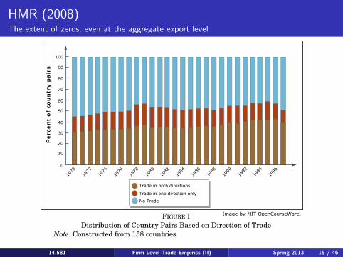
FIGURE IDistribution of Country Pairs Based on Direction of Trade

Note. Constructed from 158 countries.

only (one country imports from, but does not export to, the othercountry). As is evident from the figure, by disregarding countriesthat do not trade with each other or trade only in one direction,one disregards close to half of the observations. We show belowthat these observations contain useful information for estimatinginternational trade flows.10

Figure II shows the evolution of the aggregate real volume ofexports of all 158 countries in our sample and of the aggregatereal volume of exports of the subset of country pairs that exportedto one another in 1970. The difference between the two curvesrepresents the volume of trade of country pairs that either did nottrade or traded in one direction only in 1970. It is clear from thisfigure that the rapid growth of trade, at an annual rate of 7.5%on average, was mostly driven by the growth of trade betweencountries that traded with each other in both directions at thebeginning of the period. In other words, the contribution to the

10. Silva and Tenreyro (2006) also argue that zero trade flows can be used inthe estimation of the gravity equation, but they emphasize a heteroscedasticitybias that emanates from the log-linearization of the equation rather than theselection and asymmetry biases that we emphasize. Moreover, the Poisson methodthat they propose to use yields similar estimates on the sample of countries thathave positive trade flows in both directions and the sample of countries that havepositive and zero trade flows. This finding is consistent with our finding that theselection bias is rather small.


100

90

80

70

60

40

50

30

20

0

10

Perc

en

t o

f co

un

try p

air

s

1970

1972

1974

1976

1978

1980

1982

1984

1986

1988

1990

1992

1994

1996

No Trade

Trade in one direction only

Trade in both directions


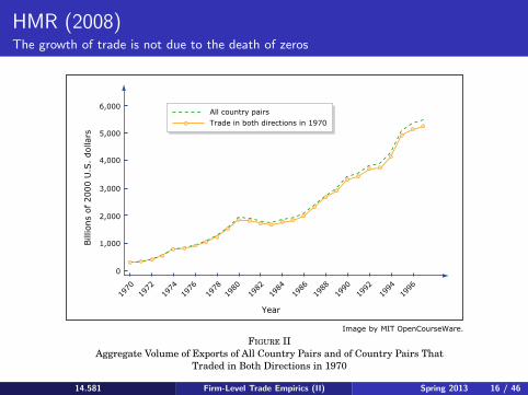
HMR (2008) The growth of trade is not due to the death of zeros

FIGURE IIAggregate Volume of Exports of All Country Pairs and of Country Pairs That

Traded in Both Directions in 1970

growth of trade of countries that started to trade after 1970 ineither one or both directions was relatively small.

Combining this evidence with the evidence from Figure I,which shows a relatively slow growth of the fraction of tradingcountry pairs, suggests that bilateral trading volumes of coun-try pairs that traded with one another in both directions at thebeginning of the period must have been much larger than the bi-lateral trading volumes of country pairs that either did not tradewith each other or traded in one direction only at the beginning ofthe period. Indeed, at the end of the period the average bilateraltrade volume of country pairs of the former type was about 35times larger than the average bilateral trade volume of countrypairs of the latter type. This suggests that the enlargement of theset of trading countries did not contribute in a major way to thegrowth of world trade.11

11. This contrasts with the sector-level evidence presented by Evenett andVenables (2002). They find a substantial increase in the number of trading partnersat the three-digit sector level for a selected group of 23 developing countries. Weconjecture that their country sample is not representative and that most of theirnew trading pairs were originally trading in other sectors. And this also contrasts


6,000

5,000

4,000

3,000

2,000

1,000

0

1970

1972

1976

1980

1984

1988

1992

1996

1974

1978

1982

1986

1990

1994

Year

Bill

ions

of 20

00 U

.S.

dolla

rs

Trade in both directions in 1970All country pairs


A Gravity Model with Zeroes

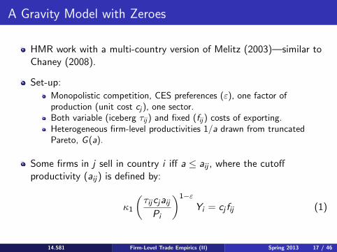
HMR work with a multi-country version of Melitz (2003)—similar to Chaney (2008).

Set-up: Monopolistic competition, CES preferences (ε), one factor of production (unit cost cj ), one sector. Both variable (iceberg τij ) and fixed (fij ) costs of exporting. Heterogeneous firm-level productivities 1/a drawn from truncated Pareto, G (a).

Some firms in j sell in country i iff a ≤ aij , where the cutoff productivity (aij ) is defined by: � �1−ετij cj aij

κ1 Yi = cj fij (1)Pi


An Augmented Gravity Equation

HMR (2008) derive a gravity equation, for those observations that are non-zero, of the form:

ln(Mij ) = β0 + αi + αj − γ ln dij + wij + uij (2)

Where: Mij is imports dij is distance wij is the ‘augmented’ part, which is a term accounting for selection. Mij = 0 is possible here (even with CES preferences and finite variable trade costs) because it is assumed that each country’s firms have productivities drawn from a bounded (truncated Pareto) distribution.


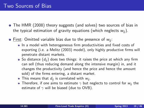
Two Sources of Bias

The HMR (2008) theory suggests (and solves) two sources of bias in the typical estimation of gravity equations (which neglects wij ).

First: Omitted variable bias due to the presence of wij : In a model with heterogeneous firm productivities and fixed costs of exporting (i.e. a Melitz (2003) model), only highly productive firms will penetrate distant markets. So distance (dij ) does two things: it raises the price at which any firm can sell (thus reducing demand along the intensive margin) in, and it changes the productivity (and hence the price and hence the amount sold) of the firms entering, a distant market. This means that dij is correlated with wij . Therefore, if one aims to estimate γ but neglects to control for wij the estimate of γ will be biased (due to OVB).


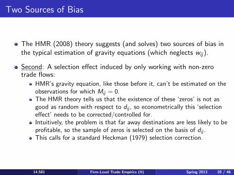
Two Sources of Bias

The HMR (2008) theory suggests (and solves) two sources of bias in the typical estimation of gravity equations (which neglects wij ).

Second: A selection effect induced by only working with non-zero trade flows:

HMR’s gravity equation, like those before it, can’t be estimated on the observations for which Mij = 0. The HMR theory tells us that the existence of these ‘zeros’ is not as good as random with respect to dij , so econometrically this ‘selection effect’ needs to be corrected/controlled for. Intuitively, the problem is that far away destinations are less likely to be profitable, so the sample of zeros is selected on the basis of dij . This calls for a standard Heckman (1979) selection correction.


HMR (2008): Two-step Estimation Two-step estimation to solve bias

1

2

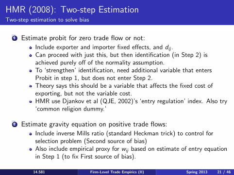
Estimate probit for zero trade flow or not: Include exporter and importer fixed effects, and dij . Can proceed with just this, but then identification (in Step 2) is achieved purely off of the normality assumption. To ‘strengthen’ identification, need additional variable that enters Probit in step 1, but does not enter Step 2. Theory says this should be a variable that affects the fixed cost of exporting, but not the variable cost. HMR use Djankov et al (QJE, 2002)’s ‘entry regulation’ index. Also try ‘common religion dummy.’

Estimate gravity equation on positive trade flows: Include inverse Mills ratio (standard Heckman trick) to control for selection problem (Second source of bias) Also include empirical proxy for wij based on estimate of entry equation in Step 1 (to fix First source of bias).


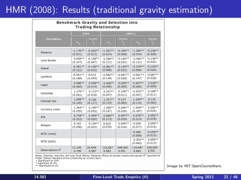
HMR (2008): Results (traditional gravity estimation)


Distance

Land border

Island

Landlock

Legal

Language

Colonial ties

Currency union

FTA

Religion

WTO (none)

WTO (both)

Observations R2

-1.176**(0.031)

-0.263**(0.012)

-1.201**(0.024)

-0.246**(0.008)

-1.200**(0.024)

-0.246**(0.008)

0.458**(0.147)

-0.148**(0.047)

0.366**(0.131)

-0.146**(0.032)

0.364**(0.131)

-0.146**(0.032)

-0.391**(0.121)

-0.136**(0.032)

-0.381**(0.096)

-0.140**(0.022)

-0.378**(0.096)

-0.140**(0.022)

-0.087**-0.561**(0.188)

-0.072(0.045)

-0.582**(0.148)

-0.087**(0.028)

-0.581**(0.147) (0.028)

0.486**(0.050)

0.038**(0.014)

0.406**(0.040)

0.029**(0.009)

0.407**(0.040)

0.028**(0.009)

1.176**(0.061)

0.113**(0.016)

0.207**(0.047)

0.109**(0.011)

0.203**(0.047)

0.108**(0.011)

1.299**(0.120)

0.128(0.117)

1.321**(0.110)

0.114(0.082)

1.326**(0.110)

0.116(0.082)

1.364**(0.255)

0.190**(0.052)

1.395**(0.187)

0.206**(0.026)

1.409**(0.187)

0.206**(0.026)

0.759**(0.222)

0.494**(0.020)

0.996**(0.213)

0.497**(0.018)

0.976**(0.214)

0.495**(0.018)

0.102(0.096)

0.104**(0.025)

-0.018(0.076)

0.099**(0.016)

-0.038(0.077)

0.098**(0.016)

-0.068(0.058)

-0.056**(0.013)

0.303**(0.042)

0.093**(0.013)

11,1460.709

24,6490.587

110,6970.682

248,0600.551

110,6970.682

248,0600.551

Variablesmij

Tij mij

Tij mij

Tij

(Porbit) (Porbit) (Porbit)

1986 1980's

Notes. Exporter, importer, and year fixed effects. Marginal effects at sample means and pseudo R2 reported for Probit. Robust standard errors (clustering by country pair).+ Significant at 10%* Significant at 5%** Significant at 1%

Benchmark Gravity and Selection into Trading Relationship


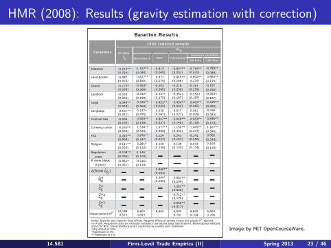
HMR (2008): Results (gravity estimation with correction)


Baseline Results

Observations R2

Distance

Island

Landlock

Legal

Language

Colonial ties

Currency union

FTA

Religion

Regulationcosts

R costs (days& proc)

Land border

0.840**(0.043)0.240*

(0.099)

-0.813(0.049)0.871

(0.170)

-0.203(0.290)-0.347*(0.175)0.431**

(0.065)-0.030(0.087)0.847**

(0.257)1.077**

(0.360)0.124

(0.227)0.120

(0.136)

6,602

-0.755**(0.070)0.892**0.170)

-0.161(0.259)-0.352+(0.187)0.407**

(0.065)-0.061(0.079)0.853**

(0.152)1.045**

(0.337)-0.141(0.250)0.073

(0.124)

6,6020.704

1.107**

-0.789**(0.088)0.863**

(0.170)-0.197(0.258)-0.353+(0.187)0.418**

(0.065)-0.036(0.083)0.838**

(0.153)

(0.346)0.065

(0.348)0.100

(0.128)

6,6020.706

(0.036)

-0.061*(0.031)

-0.108**

-0.213**(0.016)

-0.087(0.072)

-0.173*(0.078)

-0.053(0.050)

0.049**(0.019)

0.101**(0.021)

-0.009(0.130)

0.216**(0.038)

0.343**(0.009)

0.141**(0.034)

12,1980.573

1.534**

-1.146(0.100)

-0.216+(0.124)

-1.167**(0.040)0.627**

(0.165)

-0.553*(0.269)-0.432*(0.189)0.535**

(0.064)0.147+

(0.075)0.909**

(0.158)

(0.334)0.976**

(0.247)0.281*

(0.120)

6,6020.693

(0.052)-0.847**

(0.166)0.845**

(0.258)-0.218

(0.187)-0.362+

(0.064)0.434**

(0.077)-0.017

(0.148)0.848**

(0.333)1.150**

(0.197)0.241

(0.120)0.139

0.7016,602

(0.540)3.261**

(0.170)-0.712**

(0.017)0.060**

0.882**(0.209)

Variables (Probit)Tij Benchmark NLS Polynomial

50 bins 100 bins

Indicator variables

mij

1986 reduced sample

Notes: Exporter and importer fixed effects. Marginal effects at sample means and pseudo R2 reportedfor Probit. Regulation costs are excluded variables in all second stage specifications. Bootstrapped standarderrors for NLS; robust standard errors (clustering by country pair) elsewhere.+Significant at 10%.*Significant at 5%.**Significant at 1%.

*ij

*ij*ij

*ωij(from )δ

2

3

*ijη


Crozet and Koenig (CJE, 2010)

CK (2010) conduct a similar exercise to HMR (2008), but with French firm-level data.

This is attractive—after all, the main point that HMR (2008) is making is that firm-level realities matter for aggregate flows.

CK’s firm data has exports to foreign countries in it (CK focus only on adjacent countries: Belgium, Switzerland, Germany, Spain and Italy).


CK (2010): Identification

But interestingly, CK also know where the firm is in France.

So they try to separately identify the effects of variable and fixed trade costs by assuming:

Variable trade costs are proportional to distance. Since each firm is a different distance from, say, Belgium, there is cross-firm variation here. Fixed trade costs are homogeneous across France for a given export destination. (It costs just as much to figure out how to sell to the Swiss whether your French firm is based in Geneva or Normandy).


CK (2010): The model and estimation I

The model is deliberately close to Chaney (2008), which is a particular version of the Melitz (2003) model but with (unbounded) Pareto-distributed firm productivities (with shape parameter γ). We will see this model in detail in the next lecture.

In Chaney (2008) the elasticity of trade flows with respect to variable trade costs (proxies for by distance here, if we assume τij = θDij

δ

where D = distance) can be subdivided into the: EXTjExtensive elasticity: ε = −δ [γ − (σ − 1)]. CK estimate this by Dij

regressing firm-level entry (ie a Probit) on firm-level distance Dij and a firm fixed effect. This is analogous to HMR’s first stage.

INTjIntensive elasticity: ε = −δ(σ − 1). CK estimate this by regressing Dij

firm-level exports on firm-level distance Dij and a firm fixed effect. This is analogous to HMR’s second stage.


CK (2010): The model and estimation I

Recall that γ is the Pareto parameter governing firm heterogeneity.

The above two equations (HMR’s first and second stage) don’t separately identify δ, σ and γ.

So to identify the model, CK bring in another equation which is the slope of the firm size (sales) distribution.

= λ(ci )−[γ−(σ−1)]In the Chaney (2008) model this will behave as: Xi , where ci is a firm’s marginal cost and Xi is a firm’s total sales. With an Olley and Pakes (1996) TFP estimate of 1/ci , CK estimate [γ − (σ − 1)] and hence identify the entire system of 3 unknowns.


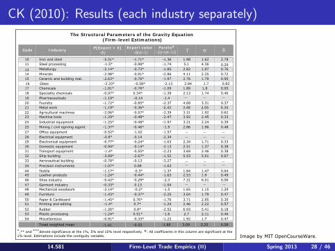
CK (2010): Results (each industry separately)


1011

1314151617181920212223242527282930313233344445464748495051525354

Glass

Textile

Rubber

Iron and steelSteel processingMetallurgyMineralsCeramic and building mat.

Speciality chemicalsPharmaceuticalsFoundryMetal work

Industrial equipmentMining / civil egnring eqpmtOffice equipmentElectrical equipmentElectronical equipment Domestic equipmentTransport equipmentShip buildingAeronautical buildingPrecision instruments

Leather productsShoe industryGarment industryMechanical woodworkFurniturePaper & CardboardPrinting and editing

Plastic processingMiscellaneous

Chemicals

Agricultural machinesMachine tools

-5.51*-1.5*-2.14*-2.98*-2.63*-2.33*-1.81*-0.97*-1.19*-1.72*-1.19*-2.06*-1.29*-1.25*-1.37*-0.52*-0.8*-0.77*-0.94*-1.4*-3.69*-0.78*-1.07*-1.17*-1.24*-0.42*-0.33*-2.14*-1.43*-1.45*-1.4*-1.26*-1.24*-0.91*

-1.41

-1.71*-0.99*-0.73*-0.91*-0.76*-0.58*

-0.76*0.34*-0.14-0.85*-0.36*-0.57*-0.48*-0.48*-0.46*-1.02-0.14-0.24*-0.14*-0.55*-2.67*-0.130.08 -0.3*-0.44*-0.29*0.13-0.2*-0.37*0.76*0.7*0.8*0.51*-0.33*

-0.53

-1.36-1.74-1.85-2.86

-2.13-1.97

-1.39-1.09

-2.37-1.4

-2.39-2.43

-1.97-2.47

-1.57-1.9

-1.63-2.34

-2.13

-1.52-2.23

-1.63-3.27

-1.63-1.37

-1.04-2.3

-2.25-1.5

-1.24-1.76

-1.6-2.52

-1.22

1.98 1.62 2.785.1 4.36 0.292.82 1.97 0.764.11 2.25 0.722.76 1.79 0.952.84 1.7 0.82

1.89 1.8 0.952.13 1.74 0.46

4.68 3.31 0.373.48 2.05 0.343.31 1.92 0.623.92 2.45 0.333.21 2.24 0.392.86 1.96 0.48

2.34 1.71 0.332.51 1.37 0.383.69 2.46 0.385.53 5.01 0.67

1.84 1.47 0.642.53 1.9 0.497.31 6.01 0.06

1.65 1.15 1.293.04 1.79 0.473.71 2.95 0.392.46 2.22 0.576.93 5.41 0.182.7 2.11 0.461.92 1.7 0.47

3.09 2.25 0.58-1.86Tread weighted mean

The Structural Parameters of the Gravity Equation (Firm-level Estimations)

Code IndustryP[Export > 0]

-δγExport value

-δ(σ−1)Pareto#

−[γ−(σ−1)] σ δγ

*,** and ***denote significance at the 1%, 5% and 10% level respectively. #: All coefficients in this column are significant at the 1% level. Estimations include the contiguity variable. Image by MIT OpenCourseWare.

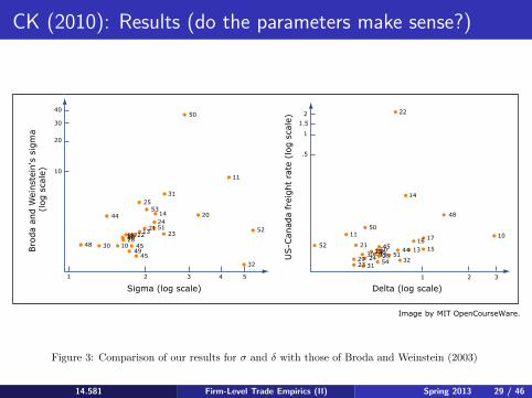
CK (2010): Results (do the parameters make sense?)

Figure 3: Comparison of our results for σ and δ with those of Broda and Weinstein (2003)

26


Bro

da a

nd W

eins

tein

's s

igm

a (

log

scal

e)

48 30

44

45

4549

102820181722

21 51

1424

5325

31

20

52

11

50

13 23

32

Sigma (log scale)1 2 3 4 5

10

20

30

40

US-C

anad

a fr

eigh

t ra

te (

log

scal

e)

.5

1

2

Delta (log scale)

1.5

1 2 3

5252

1150

21115021

2923

302431

452554

25 5144

32

13 1516 17

14

48

10

22


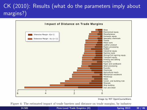
CK (2010): Results (what do the parameters imply about margins?)

Figure 4: The estimated impact of trade barriers and distance on trade margins, by industry

27


ShoeElectronical equip.MiscellaneousDomestic equip.Speciality chemicalsTextileMetal workLeather productPlastic processingRubberIndustrial equip.Machine toolsMining/Civil egnring equip.Transport equip.Printing and editingFurniturePaper and cardboardSteel processingFoundryChemicalsAgricultural mach.Mechanical woodworkMetallurgyGlassCeram. and building mat.MineralsShip buildingIron and Steel

Intensive Margin -δ(σ-1)

Extensive Margin −δ(γ−(σ−1))

6 4 2 0

Impact of Distance on Trade Margins


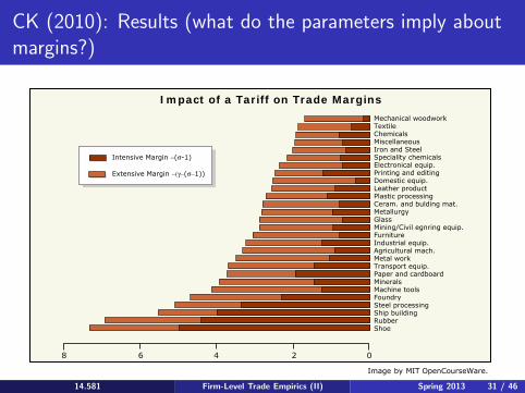
CK (2010): Results (what do the parameters imply about margins?)

Figure 4: The estimated impact of trade barriers and distance on trade margins, by industry

27


Intensive Margin −(σ-1)

Extensive Margin −(γ−(σ−1))

Mechanical woodworkTextileChemicalsMiscellaneousIron and SteelSpeciality chemicalsElectronical equip.Printing and editingDomestic equip.Leather productPlastic processingCeram. and bulding mat.MetallurgyGlassMining/Civil egnring equip.FurnitureIndustrial equip.Agricultural mach.Metal workTransport equip.Paper and cardboardMineralsMachine toolsFoundrySteel processingShip buildingRubberShoe

02468

Impact of a Tariff on Trade Margins


Eaton, Kortum and Kramarz (2009)

EKK (2009) construct a Melitz (2003)-like model in order to try to capture the key features of French firms’ exporting behavior:

Whether to export. (Simple extensive margin). Which countries to export to. (Country-wise extensive margins). How much to export to each country. (Intensive margin).

They uncover some striking regularities in the firm-wise sales data in (multiple) foreign markets.

These ‘power law’ like relationships occur all over the place (Gabaix (ARE survey, 2009)). Most famously, they occur for domestic sales within one market. In that sense, perhaps it’s not surprising that they also occur market by market abroad. (At the heart of power laws is scale invariance.)


EKK (2009): Stylised Fact 1: Market Entry (averagesacross countries)‘Normalization’: NnF/(XnF/Xn)

FRA

BELNET

GER

ITAUNK

IREDENGREPOR

SPA

NORSWE

FIN

SWI

AUT

YUGTUR

USR

GEECZEHUN

ROMBUL

ALB

MOR ALGTUN

LIY

EGY

SUD

MAUMAL BUKNIG

CHA

SEN

SIELIB

COT

GHA

TOGBENNIA

CAM

CEN ZAI

RWABURANG

ETH

SOM

KEN

UGA

TANMOZ

MAD MAS

ZAMZIM

MAW

SOU

USA

CAN

MEX

GUAHONELSNICCOS

PANCUBDOM

JAMTRI

COLVEN

ECUPER

BRACHI

BOL

PARURU

ARGSYR IRQIRN

ISR

JOR

SAUKUW

OMA

AFG

PAKIND

BANSRI

NEP

THA

VIE

INOMAY

SIN

PHICHN

KOR

JAP

TAI

HOK AUL

PAP

NZE

10

100

1000

10000

100000

# fir

ms

sellin

g in

mar

ket

.1 1 10 100

1000

10000market size ($ billions)

Panel A: Entry of Firms

FRABELNET

GER

ITAUNK

IREDENGRE

POR

SPANORSWEFIN

SWIAUT

YUG

TUR

USR

GEE

CZEHUN

ROMBUL

ALB MORALG

TUN

LIY

EGYSUD

MAU

MAL

BUK

NIGCHA

SEN

SIE

LIB

COT

GHA

TOGBEN

NIA

CAM

CEN

ZAI

RWABUR

ANGETH

SOM KENUGA

TAN

MOZMAD

MAS

ZAM

ZIM

MAW

SOU

USA

CAN

MEX

GUAHONELS

NIC

COS PANCUB

DOMJAM

TRICOL

VENECU PER

BRA

CHI

BOL PARURU

ARG

SYR

IRQ

IRN

ISR

JOR

SAU

KUWOMA

AFG

PAK

IND

BANSRI

NEP

THA

VIEINO

MAYSINPHI

CHN

KOR

JAP

TAI

HOK

AUL

PAP

NZE

1000

10000

100000

1000000

5000000

entry

nor

mal

ized

by

Fren

ch m

arke

t sha

re

.1 1 10 100 100010000

market size ($ billions)

Panel B: Normalized Entry

FRA

BELNET

GERITA UNK

IREDENGREPOR

SPANOR

SWEFIN SWIAUT

YUGTUR

USRGEE

CZEHUNROM

BUL

ALB

MOR

ALG

TUN

LIYEGY

SUDMAUMAL BUKNIG

CHASEN

SIE

LIB COTGHATOGBEN

NIA

CAM

CEN

ZAI

RWABUR

ANGETH

SOM

KENUGA TAN

MOZMAD MAS

ZAMZIM

MAWSOU

USA

CANMEX

GUAHONELS

NIC

COSPAN

CUB

DOM

JAMTRI

COLVEN

ECUPER

BRA

CHI

BOL

PARURU

ARGSYR

IRQIRN

ISRJOR

SAU

KUWOMA

AFG PAKIND

BANSRINEP

THAVIE

INO

MAYSINPHI

CHN

KOR JAPTAIHOK

AUL

PAP NZE

.001

.01

.1

1

10

perc

entil

es (2

5, 5

0, 7

5, 9

5) b

y m

arke

t ($

milli

ons)



Figure 1: Entry and Sales by Market Size




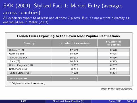
EKK (2009): Stylised Fact 1: Market Entry (averages across countries) All exporters export to at least one of these 7 places. But it’s not a strict hierarchy as one would see in Melitz (2003).


French Firms Exporting to the Seven Most Popular Destinations

Belgium* (BE)Germany (DE)

Switzerland (CH)

Italy (IT)

United Kingdom (UK)

Netherlands (NL)

United States (US)

Total Exporters

* Belgium includes Luxembourg

Number of exporters

17,69914,579

14,173

10,643

9,752

8,294

7,608

34,035

Fraction of exporters

0.5200.428

0.416

0.313

0.287

0.244

0.224

Country


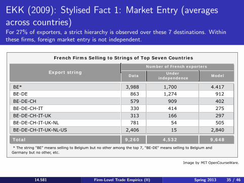
EKK (2009): Stylised Fact 1: Market Entry (averages across countries) For 27% of exporters, a strict hierarchy is observed over these 7 destinations. Within these firms, foreign market entry is not independent.


Export string

9,260 4,532

BE* 3,988 1,700 4.417BE-DE 863 1,274 912BE-DE-CH 579 909 402BE-DE-CH-IT 330 414 275BE-DE-CH-IT-UK 313 166 297BE-DE-CH-IT-UK-NL 781 54 505BE-DE-CH-IT-UK-NL-US 2,406 15 2,840

9,648Total

* The string "BE" means selling to Belgium but no other among the top 7, "BE-DE" means selling to Belgium and Germany but no other, etc.

DataUnder

independenceModel

French Firms Selling to Strings of Top Seven Countries

Number of French exporters


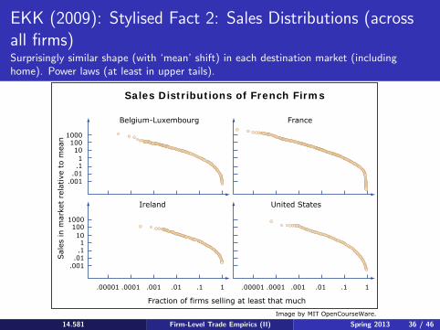
EKK (2009): Stylised Fact 2: Sales Distributions (across all firms) Surprisingly similar shape (with ‘mean’ shift) in each destination market (including home). Power laws (at least in upper tails).


1000100101

.1

.001.01

1000100101

.1

.001.01

.00001 .00001.0001 .0001.001 .001.01 .01.1 .11 1

Fraction of firms selling at least that much

Sal

es in

mar

ket

rela

tive

to m

ean

Sales Distributions of French Firms

Belgium-Luxembourg France

United StatesIreland


EKK (2009): Stylised Fact 3: Export Participation and Size in France Big firms at home are multi-destination exporters.


1

1

2

2

3

34

45

56

6798

798123456789

123456789

123456789

123456789

123456789

123456789

123456789

123456789

123456789

123456789

123456789

123456789

123456789

123456789

123456789123456789

123456789

123456789

123456789

123456789

123456789123456789

123456789123456789123456789

123451234512345123451234512345

1234512345

12345123451234512345

110 1081051000

1000

100

10

11 10 100 1000 10000 10000 500000

#Firms selling to k or more market

Sales and # Penetrating Multiple Markets

NEPAFG

AFGBRIJANJAW

TANTRYCHA

DELBRABRASEBSEB

FRA

AFGPANLMBNEP AFGPAN

PANCHADELDELBRALMB

NEPAFGPAN

CHACHACHA

CHACHACHACHA

DELDELDELDEL

BRASEBLMBNEPAFG

PANCHADELBRASEB

LMBLMB

LMBLMB

LMBNEPAFGPANCHADELBRASEBSEB LMB

NEPAFGPANCHADELBRASEBLMBNEPAFG

PANCHACHA DELBRASEBLMBNEPAFGPANCHADELBRASEB

LMBNEPAFG

PANCHADELBRASEBLMBNEPAFG


PANCHADELBRASEBLMBNEPNEPAFG

PAN

20 100 1000 10000 100000 500000

.1

1

10

100

1000

10000

#Firms selling in the market

Distribution of Sales and Market Entry

1000

1000

100

10

1

1 2 4 8 16 32 64 128Minimum number of markets penetrated

Sales and Markets Penetrated

Aver

age

sale

in F

ranc

e (

$ m

illio

ns)

NEP

AFGPAN

FRA

LMBNEPAFG


PANCHADEL

BRA

SEBLMBNEP

CHADELBRASEBSEB

DELBRABRASEB

AFGBRALMBNEPAFG

PANCHADELBRALMBNEPAFG

PANCHADELBRASEB

AFGBRALMBNEPAFG

PANCHABRASEB SEBSEBSEBSEB

AFGBRALMBNEPAFG

PANCHADELBRASEBLMBNEP

PANCHADELBRASEBSEB

AFGBRALMBAFGPANCHADELBRALMBNEPAFG

PANCHADELBRASEBLMB

AFGBRALMBNEPAFG

PANCHADELBRASEBLMBAFGPANCHADELBRA

LMB

NEPPANCHADEL

1000

100

10

120 100 1000 10000 100000 500000


Sales and # Selling to a Market

Aver

age

sale

s in

Fra

nce

($ m

illio

ns)

Aver

age

sale

in F

ranc

e ($

mill

ions

)Pe

rcen

tiles

(25

, 50

, 75

, 95

) in

Fr

ance

($

mill

ions

)

Sales in France and Market Entry


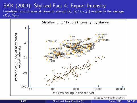
EKK (2009): Stylised Fact 4: Export Intensity Firm-level ratio of sales at home to abroad (XnF (j)/XFF (j)) relative to the average (X̄nF /X̄FF )


AFG NIC

PAP

ALBNEP MAW

UGASOM

USR

CUB

GEE

PAR

JAM

BOLELS

RWASUD

SUD

ROM

ROMROM

COL

CHN

KOR

EGY

EGY

BRABRABRA

BRA

CENTOG

CRA

MOZIRN

SENCOI

LIY

LIBVIE IREISR

KORIND

COSCOS

SIEHONZIM GENJOR

COTCOTCOT COT

CORCORJAMTMRTMR

TMR TMR

CANCANCAN

CANCANCANCANCANCANCANCANCANCAN

CANCANCAN

CANCANCAN

HONHON

HON

SAUJAPALG

COLCOL

BRACOL

GUA

PAN

NETSPA

SWEBELUNKITK

USA GER

.0001

.001

.01

.1

1

10 100 1000 10000 100000# Firms selling in the market

Perc

entil

es (

50,9

5) o

f no

rmal

ized

ex

port

inte

nsity

Distribution of Export Intensity, by Market


EKK (2009): Model

The above relationships fit the Melitz (2003) model (with G (.) being Pareto) in some regards, but not all.

EKK (2009) therefore add some features to Melitz (2003) in order to bring this model closer to the data.

Most of these will take the flavor of ‘firm-specific shocks/noise’. The shocks smooths things out, allows for unobserved heterogeneity, and answer the structural econometrician’s question of “where does your regression’s error term come from?”.

The remaining slides describe some of the features of the EKK model, and how the model matches the data. I include them here just for your interest as they won’t make much sense until you’ve learned the Melitz (2003) model—see the next lecture!


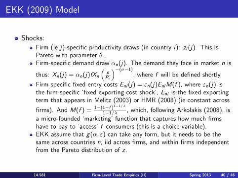
EKK (2009) Model

Shocks: Firm (ie j)-specific productivity draws (in country i): zi (j). This is Pareto with parameter θ. Firm-specific demand draw αn(j). The demand they face in market n is −(σ−1)

pthus: Xn(j) = αn(j)fXn Pn, where f will be defined shortly.

Firm-specific fixed entry costs Eni (j) = εn(j)Eni M(f ), where εn(j) is the firm-specific ‘fixed exporting cost shock’, Eni is the fixed exporting term that appears in Melitz (2003) or HMR (2008) (ie constant across

1−(1−f )1−1/λ

firms). And M(f ) = , which, following Arkolakis (2008), is 1−1/λ a micro-founded ‘marketing’ function that captures how much firms have to pay to ‘access’ f consumers (this is a choice variable). EKK assume that g(α, ε) can take any form, but it needs to be the same across countries n, iid across firms, and within firms independent from the Pareto distribution of z .


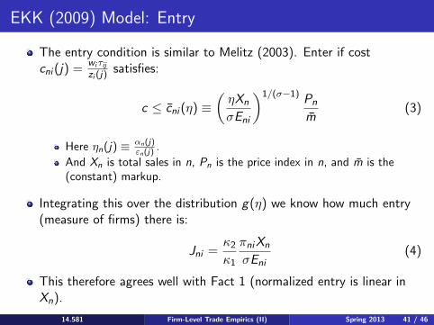
EKK (2009) Model: Entry

The entry condition is similar to Melitz (2003). Enter if cost wi τijcni (j) = satisfies: zi (j)

(3)

Here ηn(j) ≡ αn (j) .εn (j) And Xn is total sales in n, Pn is the price index in n, and m̄ is the (constant) markup.

Integrating this over the distribution g(η) we know how much entry (measure of firms) there is:

κ2 πni XnJni = (4)

κ1 σEni

This therefore agrees well with Fact 1 (normalized entry is linear in Xn).


c ≤ c̄ni (η) ≡(ηXn

σEni

)1/(σ−1) Pn

m̄

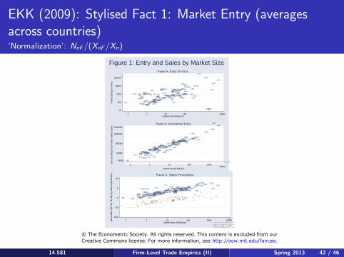
EKK (2009): Stylised Fact 1: Market Entry (averages across countries) ‘Normalization’: NnF /(XnF /Xn)

FRA

BELNET

GER

ITAUNK

IREDENGREPOR

SPA

NORSWE

FIN

SWI

AUT

YUGTUR

USR

GEECZEHUN

ROMBUL

ALB

MOR ALGTUN

LIY

EGY

SUD

MAUMAL BUKNIG

CHA

SEN

SIELIB

COT

GHA

TOGBENNIA

CAM

CEN ZAI

RWABURANG

ETH

SOM

KEN

UGA

TANMOZ

MAD MAS

ZAMZIM

MAW

SOU

USA

CAN

MEX

GUAHONELSNICCOS

PANCUBDOM

JAMTRI

COLVEN

ECUPER

BRACHI

BOL

PARURU

ARGSYR IRQIRN

ISR

JOR

SAUKUW

OMA

AFG

PAKIND

BANSRI

NEP

THA

VIE

INOMAY

SIN

PHICHN

KOR

JAP

TAI

HOK AUL

PAP

NZE

10

100

1000

10000

100000

# fir

ms

sellin

g in

mar

ket

.1 1 10 100

1000

10000market size ($ billions)

Panel A: Entry of Firms

FRABELNET

GER

ITAUNK

IREDENGRE

POR

SPANORSWEFIN

SWIAUT

YUG

TUR

USR

GEE

CZEHUN

ROMBUL

ALB MORALG

TUN

LIY

EGYSUD

MAU

MAL

BUK

NIGCHA

SEN

SIE

LIB

COT

GHA

TOGBEN

NIA

CAM

CEN

ZAI

RWABUR

ANGETH

SOM KENUGA

TAN

MOZMAD

MAS

ZAM

ZIM

MAW

SOU

USA

CAN

MEX

GUAHONELS

NIC

COS PANCUB

DOMJAM

TRICOL

VENECU PER

BRA

CHI

BOL PARURU

ARG

SYR

IRQ

IRN

ISR

JOR

SAU

KUWOMA

AFG

PAK

IND

BANSRI

NEP

THA

VIEINO

MAYSINPHI

CHN

KOR

JAP

TAI

HOK

AUL

PAP

NZE

1000

10000

100000

1000000

5000000

entry

nor

mal

ized

by

Fren

ch m

arke

t sha

re

.1 1 10 100 100010000

market size ($ billions)

Panel B: Normalized Entry

FRA

BELNET

GERITA UNK

IREDENGREPOR

SPANOR

SWEFIN SWIAUT

YUGTUR

USRGEE

CZEHUNROM

BUL

ALB

MOR

ALG

TUN

LIYEGY

SUDMAUMAL BUKNIG

CHASEN

SIE

LIB COTGHATOGBEN

NIA

CAM

CEN

ZAI

RWABUR

ANGETH

SOM

KENUGA TAN

MOZMAD MAS

ZAMZIM

MAWSOU

USA

CANMEX

GUAHONELS

NIC

COSPAN

CUB

DOM

JAMTRI

COLVEN

ECUPER

BRA

CHI

BOL

PARURU

ARGSYR

IRQIRN

ISRJOR

SAU

KUWOMA

AFG PAKIND

BANSRINEP

THAVIE

INO

MAYSINPHI

CHN

KOR JAPTAIHOK

AUL

PAP NZE

.001

.01

.1

1

10

perc

entil

es (2

5, 5

0, 7

5, 9

5) b

y m

arke

t ($

milli

ons)



Figure 1: Entry and Sales by Market Size



EKK (2009) Model: Firm Sales

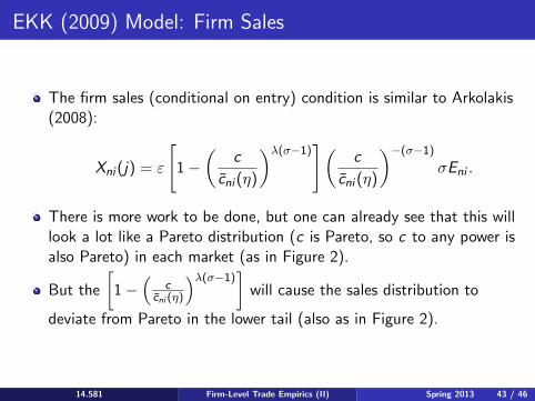
The firm sales (conditional on entry) condition is similar to Arkolakis (2008):

There is more work to be done, but one can already see that this will look a lot like a Pareto distribution (c is Pareto, so c to any power is also Pareto) in each market (as in Figure 2).

deviate from Pareto in the lower tail (also as in Figure 2).


Xni (j) = ε

[1−

(c

c̄ni (η)

)λ(σ−1)](

c −

c̄ni (η)

) (σ−1)

σEni .

But the

[1−

(c

c̄ni (η)

)λ(σ−1)]

will cause the sales distribution to

EKK (2009): Stylised Fact 2: Sales Distributions (across all firms) Surprisingly similar shape (with ‘mean’ shift) in each destination market (including home). Power laws (at least in upper tails).


1000100101

.1

.001.01

1000100101

.1

.001.01

.00001 .00001.0001 .0001.001 .001.01 .01.1 .11 1

Fraction of firms selling at least that much

Sal

es in

mar

ket

rela

tive

to m

ean

Sales Distributions of French Firms

Belgium-Luxembourg France

United StatesIreland


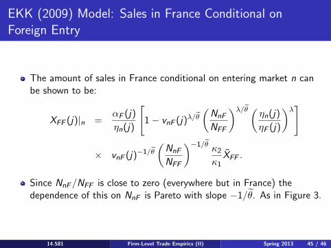
EKK (2009) Model: Sales in France Conditional on Foreign Entry

The amount of sales in France conditional on entering market n can be shown to be:

Since NnF /NFF is close to zero (everywhere but in France) the dependence of this on NnF is Pareto with slope −1/θB. As in Figure 3.


XFF (j)|n =αF (j) N

1ηn(j)

[− vnF (j)λ/θ̃

(nF

NFF

)λ/θ̃ ( ηn(j)

ηF (j)

)λ]

× vnF (j)−1/θ̃

(NnF

NFF

)−1/θ̃ κ2

κ1X̄FF .

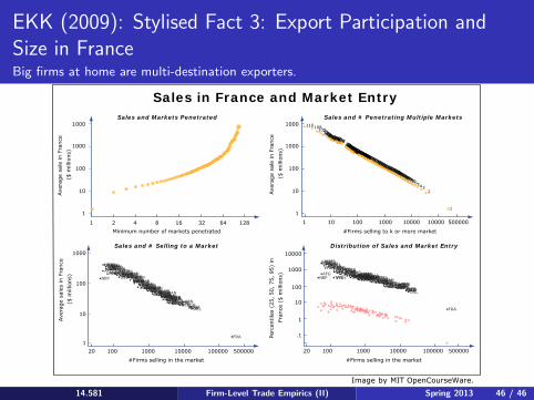
EKK (2009): Stylised Fact 3: Export Participation and Size in France Big firms at home are multi-destination exporters.


1

1

2

2

3

34

45

56

6798

798123456789

123456789

123456789

123456789

123456789

123456789

123456789

123456789

123456789

123456789

123456789

123456789

123456789

123456789

123456789123456789

123456789

123456789

123456789

123456789

123456789123456789

123456789123456789123456789

123451234512345123451234512345

1234512345

12345123451234512345

110 1081051000

1000

100

10

11 10 100 1000 10000 10000 500000

#Firms selling to k or more market

Sales and # Penetrating Multiple Markets

NEPAFG

AFGBRIJANJAW

TANTRYCHA

DELBRABRASEBSEB

FRA

AFGPANLMBNEP AFGPAN

PANCHADELDELBRALMB

NEPAFGPAN

CHACHACHA

CHACHACHACHA

DELDELDELDEL

BRASEBLMBNEPAFG

PANCHADELBRASEB

LMBLMB

LMBLMB

LMBNEPAFGPANCHADELBRASEBSEB LMB

NEPAFGPANCHADELBRASEBLMBNEPAFG

PANCHACHA DELBRASEBLMBNEPAFGPANCHADELBRASEB

LMBNEPAFG



PANCHADELBRASEBLMBNEPNEPAFG

PAN

20 100 1000 10000 100000 500000

.1

1

10

100

1000

10000


Distribution of Sales and Market Entry

1000

1000

100

10

1

1 2 4 8 16 32 64 128Minimum number of markets penetrated

Sales and Markets Penetrated

Aver

age

sale

in F

ranc

e (

$ m

illio

ns)

NEP

AFGPAN

FRA

LMBNEPAFG


PANCHADEL

BRA

SEBLMBNEP

CHADELBRASEBSEB

DELBRABRASEB

AFGBRALMBNEPAFG

PANCHADELBRALMBNEPAFG

PANCHADELBRASEB

AFGBRALMBNEPAFG

PANCHABRASEB SEBSEBSEBSEB

AFGBRALMBNEPAFG

PANCHADELBRASEBLMBNEP

PANCHADELBRASEBSEB

AFGBRALMBAFGPANCHADELBRALMBNEPAFG

PANCHADELBRASEBLMB

AFGBRALMBNEPAFG

PANCHADELBRASEBLMBAFGPANCHADELBRA

LMB

NEPPANCHADEL

1000

100

10

120 100 1000 10000 100000 500000


Sales and # Selling to a Market

Aver

age

sale

s in

Fra

nce

($ m

illio

ns)

Aver

age

sale

in F

ranc

e ($

mill

ions

)Pe

rcen

tiles

(25

, 50

, 75

, 95

) in

Fr

ance

($

mill

ions

)

Sales in France and Market Entry


MIT OpenCourseWarehttp://ocw.mit.edu

14.581 International Economics ISpring 2013

For information about citing these materials or our Terms of Use, visit: http://ocw.mit.edu/terms.

http://ocw.mit.edu

http://ocw.mit.edu/terms.

international trade — — | | 13: firm-level trade empirics (ii) · lecture 13: firm-level trade...

Documents