international trade finance and the cost channel of
TRANSCRIPT

International Trade Finance and the CostChannel of Monetary Policy in Open
Economies∗
Nikhil PatelInternational Monetary Fund
This paper studies the role of international trade financein the transmission mechanism of monetary policy in atwo-country dynamic stochastic general equilibrium (DSGE)framework. The model shows that trade finance can bothamplify or mitigate the impact of shocks, depending on thedegree to which countries differ in price stickiness and depen-dence on trade finance. The model is estimated with Bayesiantechniques using macroeconomic data from the United Statesand the euro zone and reveals the impact of trade finance tobe quantitatively important, especially for spillover effects ofshocks across countries. It significantly alters the interpretationof the sources and propagation of business cycles. In particular,accounting for trade finance makes external shocks much lessimportant for business cycles in the euro area. At the sametime, spillover effects of U.S. monetary policy on euro-areaoutput are much larger.
JEL Codes: F44, F41, E44, E52.
∗I am grateful to Shang-Jin Wei, Stephanie Schmitt-Grohe, and Martin Uribefor extensive guidance. I would also like to thank Boragan Aruoba and twoanonymous referees for extensive comments, and Scott Davis, Michael Devereux,Keshav Dogra, Torsten Ehlers, Yang Jiao, Frederic Mishkin, Emi Nakamura,Jaromir Nosal, Christopher Otrok, Pablo Ottonello, Ricardo Reis, Jon Steinsson,David Weinstein, James Yetman, and seminar participants at various institu-tions for valuable comments and discussions. Part of this research was conductedwhen I was visiting the Hong Kong Monetary Authority (HKMA) and HongKong Institute for Monetary Research (HKIMR). I am grateful to them for theirhospitality and support. The views expressed here are those of the author and donot necessarily correspond to those of the IMF, HKIMR, or HKMA. All errorsare the sole responsibility of the author. Author contact: [email protected].
117

118 International Journal of Central Banking October 2021
1. Introduction
While the literature on trade finance is extensive,1 the implicationsof trade finance for business cycle fluctuations in macroeconomicmodels remain understudied. This omission is conspicuous given thefact that open-economy models that are commonly used for pol-icy analysis and forecasting typically give a central role to inter-national trade. Indeed, trade is the primary and in some cases theonly channel through which shocks can be transmitted across coun-tries in these models.2 This paper studies business cycle implicationsof trade finance through the lens of an estimated two-country NewKeynesian dynamic stochastic general equilibrium (DSGE) model.
The term “trade finance” is used in the literature to describea number of different financing arrangements. These include directlending by banks to the exporter and/or the importer, interfirmtrade credit, open account (i.e., post-delivery payment), or cash inadvance.3 Recognizing that all these mechanisms involve at leastone of the parties engaging in borrowing at an interest rate that ispotentially affected by changes in monetary policy, trade finance inthe paper is introduced by augmenting the cost channel of monetarypolicy. While there exists a sizable literature that studies differentaspects of the cost channel of monetary policy, including extensionsto open-economy settings (see, for instance, Gertler, Gilchrist, andNatalucci 2007 and Gilchrist 2003), these models do not distinguishbetween the external finance dependence of international and intra-national trade, a distinction that the international trade literaturehas strongly emphasized. This paper models this distinction andshows that it is important not only quantitatively but also quali-tatively in terms of the sign of the effects that the cost channel ofmonetary policy can generate.
1Bekaert and Hodrick (2017) identify trade finance as the “fundamental prob-lem in international trade.” According to the estimates of the Committee on theGlobal Financial System (CGFS), $6.5–8 trillion worth of bank-intermediatedtrade finance was provided during the year 2011, which, at around 10 percent ofglobal gross domestic product (GDP) and 30 percent of global trade, is a fairlysizable number in itself, even though it does not include letters of credit andother forms of trade finance not explicitly involving bank loans.
2See, for instance, Christiano, Eichenbaum, and Evans (2005) and Smets andWouters (2003).
3See Ahn, Amiti, and Weinstein (2011) and Schmidt-Eisenlohr (2013).

Vol. 17 No. 4 International Trade Finance and the Cost Channel 119
The standard cost channel of monetary policy typically ampli-fies the output effect of domestic shocks that hit the economy.4 Onthe other hand, this paper shows that the cost channel when com-bined with trade finance can either amplify or mitigate the effectsof shocks. Consider a monetary contraction in the home economy,which leads to a fall in domestic aggregate demand and prices. Ifimporting firms are constrained to borrow at their respective homeinterest rates, then foreign imports into the home country becomemore expensive, whereas imports into the foreign country (i.e., homeexports) become cheaper for foreign consumers, leading to a higherdemand for the latter and a lower demand for the former. As a result,the trade finance plays the role of cushioning the effect of the originalmonetary contraction on home output. If on the other hand export-ing firms (instead of importing firms) are financially constrained andborrow in their domestic interest rate, then the trade finance con-straints can amplify the effect of the monetary contraction on homeGDP in the example just described.
Elaborating on these points, the first part of the paper focuseson studying the impact of trade finance on the transmission mecha-nism of monetary policy shocks through simulations under alter-nate scenarios. It illustrates how the effect depends critically onparameters characterizing the trade sector in the model, includ-ing the degree of price stickiness (and asymmetry across coun-tries in this parameter) and parameters quantifying the externalfinance dependence of trade flows. Various sources of this asym-metry are identified and their implications are explored. Moreover,because monetary policy has both an exogenous and endogenouscomponent, these additional features not only affect the propaga-tion of monetary policy shocks themselves but also the propaga-tion of all other shocks via the endogenous component of monetarypolicy.
The general nature of the implications that emerge from themodel can be summarized under two polar scenarios depending onwhether the countries are symmetric with respect to each other inregard to their external sectors. External sectors could differ dueto the degree of external finance dependence, price flexibility, and
4See, for instance, Barth and Ramey (2002).

120 International Journal of Central Banking October 2021
currency denomination of trade finance contracts, all of which inturn could be functions of the nature of export bundles of countries.When the external sectors are symmetric across countries, incorpora-tion of trade finance leads to sharp movements in trade volumes buthas negligible impact on GDP. When global interest rates are high,international trade becomes more expensive, which leads to higherimport prices for both countries. Both countries shift away fromimports and towards their respective domestically produced goodsin such a way that the net effect on the GDP of both countries isminimal. On the other hand, when countries are asymmetric in anyof these dimensions, the demand shifts do not offset one another, andtrade finance can significantly alter the response of GDP to variousshocks that hit the economy.
Given that these parameters play a critical role in affecting busi-ness cycle fluctuations and for the most part extant literature is notvery informative on their values, uncovering values of these parame-ters and relative differences across trading partners is likely to bea fruitful avenue for future research. The second part of the papertakes the first step in this direction by estimating a two-countryDSGE model with trade finance using data from two regions thatconstitute one of the largest trading relationships in the world—theUnited States and the euro zone (EZ). The focus of the estimationexercise is threefold: (i) parameter estimation, (ii) model compar-ison, and (iii) a quantitative analysis of the role played by tradefinance in business cycle fluctuations. Regarding parameter estima-tion, the estimates reveal asymmetries in the degree of price sticki-ness in imports between the United States and the European Union(EU). In particular, retail prices of U.S. imports are found to bemore flexible than their European counterparts.
While open-economy macro models typically give a central roleto international trade, by omitting trade finance they ignore animportant feature of international trade which has been shown to beimportant in the trade literature. How significant is this omission,and should there be a move towards incorporating models involv-ing trade finance? To this end, estimation of different versions ofthe model (in particular, ones with and without trade finance) pro-vide strong evidence in favor of models incorporating trade financeand show that trade finance is indeed quantitatively important inaccounting for business cycle fluctuations.

Vol. 17 No. 4 International Trade Finance and the Cost Channel 121
The model makes the simplifying assumption that exporters andimporters are not allowed to switch between sources of funding inresponse to shocks. While there is an extensive literature document-ing that firms’ sources of funding are sticky, some recent studiesfocusing specifically on international trade finance have found thatthat exporters and importers do indeed change their sources of fund-ing in response to shocks.5 The implications of such switching arediscussed below, while modeling optimal funding choice remains afruitful avenue for future research.
The remainder of this paper is organized as follows. Section 2begins with a brief literature review. Section 3 lays out the main fea-tures of the model and discusses the equilibrium conditions. Section4 presents a calibration- and simulation-based exercise to illustratedifferent features of the model. Section 5 undertakes Bayesian esti-mation of the model, and section 6 concludes.
2. Related Literature
This paper is linked to several different strands in the literature atthe intersection of macroeconomics, monetary economics, and inter-national trade. The incorporation of credit constraints in this paperis motivated by the extensive empirical literature on trade financeand its link to monetary policy. This literature has documented—across countries and time—the higher reliance of international tradeon external finance compared with intranational trade. Ju, Lin, andWei (2013) employ a large bilateral sector-level trade data set forthe years 1970–2000 to study the effect of monetary policy tight-ening on export behavior. They find that the sectors relying moreon external finance are disproportionally largely affected by mon-etary tightening, and that the exporting behavior is affected morethan domestic sales. Using monthly data on U.S. imports, Chor andManova (2012) find that the United States imported less from coun-tries with higher interest rates and tighter credit conditions. Using apanel of 91 countries from 1980 to 1997, Manova (2008) shows thatequity market liberalizations are positively associated with higherexports. Manova, Wei, and Zhang (2011) report similar results using
5See, for instance, Antras and Foley (2015), Demir and Javorcik (2018), andGarcia-Marin, Justel, and Schmidt-Eisenlohr (2019).

122 International Journal of Central Banking October 2021
firm-level data from China. Based on survey data from Italian manu-facturing firms, Minetti and Zhu (2011) report that credit rationingaffects international sales more than domestic sales. Using a detailedmatched firm-level data set for banks and firms in Japan, Amitiand Weinstein (2009) find that the health of the banking sector ismuch more influential in determining exporting behavior of firmscompared with their domestic sales.
On the theoretical front, several explanations for this phenome-non have been explored in the literature. The most common expla-nation hinges on the fact that international shipments take moretime than domestic shipments (both travel time and time takenfor documentation and clearances),6 which implies that producershave to incur costs of production much before revenues are obtained.Feenstra, Li, and Yu (2014) provide a theoretical model incorporat-ing these ideas. International trade is also likely to be more inten-sive in external finance because of higher information asymmetriesassociated with cross-border transactions.
Recognizing the need for trade finance, there is also a grow-ing literature on the optimal financing arrangement. In theoreticalframeworks, Ahn (2014) and Schmidt-Eisenlohr (2013) study howthe optimal financing arrangement depends on the financial mar-ket characteristics of both the source and the destination country.Ahn, Khandelwal, and Wei (2011), Hoefele, Schmidt-Eisenlohr, andYu (2016), and Niepmann and Schmidt-Eisenlohr (2017) test theoccurrences of different financing arrangements in the data againstthese theories and find the evidence to be broadly consistent. Cus-tom data suggest that open account is the dominant financing form,with a share of around 80 percent of trade reported for Turkey, Chile,and Colombia in Ahn, Khandelwal, and Wei (2011) and Demir andJavorcik (2018).7 For the United States, Antras and Foley (2015)also find a large role for cash in advance when looking at thetransaction-level data from a U.S. exporter of frozen and refrigeratedfood products.
6See Djankov, Freund, and Pham (2006) and Hummels and Schaur (2013).7This share, although high, is still less than estimates of the share of open
account in domestic transactions in advanced economies. Ellingsen, Jacobson,and von Schedvin (2016), for instance, find the open account share to be close to100 percent for domestic transactions in Sweden.
Vol. 17 No. 4 International Trade Finance and the Cost Channel 123
An alternative to bank-intermediated trade finance is tradecredit, or the direct extension of credit between buyers and sup-pliers. Although the two are substitutes and one would expect firmsto turn from bank-intermediated trade finance to trade credits, theevidence supporting this hypothesis is mixed.8
In its exploration of the role of the cost channel of monetarypolicy in open-economy settings, the paper has several precedentsin the closed-economy literature. Using industry-level data from theUnited States, Barth and Ramey (2002) provide compelling evidencein favor of the cost channel of monetary policy. Dedola and Lippi(2005) report similar conclusions based on a richer data set con-taining information on 21 manufacturing sectors from five OECDcountries. Ravenna and Walsh (2006) highlight the presence of thecost channel on the basis of parameters estimates based on theirestimation of the Phillips curve for the United States. They alsoprovide a characterization of the optimal monetary policy problemin the presence of these cost side effects. In advanced economiesmonetary policy is primarily conducted via open market operationswhich affect the balance sheets of banks directly. If cost side effectsof monetary policy are present, one would expect countries withbank-based systems to be more sensitive to monetary policy shocks.This is exactly what Cecchetti (1999) and Kashyap and Stein (1997)find. Moreover, based on joint BIS-IMF-OECD-World Bank statis-tics on external debt, Auboin (2007) documents that 80 percent ofthe providers of trade finance are private banks.9
The paper also builds on ideas developed in the literature on ver-tical specialization and multiple-stage production. Huang and Liu(2001, 2007) and Wong and Eng (2013) are among the many papersthat have used these features to explain various empirical stylizedfacts that standard models have difficulty accounting for. This paperbuilds a model that would allow multiple-stage trade intermediationto act as an amplification mechanism for shocks due to borrowingconstraints. Similar ideas incorporating liquidity constraints have
8See Asmundson et al. (2011) and Choi and Kim (2005) as two examples ofthe mixed evidence.
9In the Lehman bankruptcy 6 of the 30 largest unsecured claims againstLehman were letters of credit.

124 International Journal of Central Banking October 2021
been applied in a closed-economy setting by Bigio and La’O (2013)and Kalemli-Ozcan et al. (2013).
3. Model
The model in this paper builds on the framework used in Galı andMonacelli (2005) and Lubik and Schorfheide (2006), which in turnfit into the New Open Economy Macroeconomics (NOEM) para-digm of Obstfeld, Rogoff, and Wren-Lewis (1996).10 In particular,it builds on Lubik and Schorfheide (2006) by modeling a cost chan-nel of monetary policy and allowing for trade finance and multiplestages in production of exports. Apart from these features (whichare limited to the import-export sector), the rest of the model isidentical to Lubik and Schorfheide (2006).
The world economy is assumed to comprise two countries ofequal size. Households have preferences over domestic and foreigngoods and supply labor to firms. There are two sets of firms in eacheconomy—production firms and trade firms. Prices are assumed tobe sticky in both the domestic and import sector. The monetaryauthority uses the short-term nominal interest rate as its instru-ment. For brevity, only the home economy is described in detailbelow. The foreign economy is assumed to be isomorphic.
3.1 Households
The household side of the economy is characterized by a representa-tive consumer with preferences over consumption and leisure givenby the following utility function:
U(Cht , Hh
t , Nht ) =
11 − σc
(Ch
t − Hht
At
)1−σc
− 11 + σL
Nh1+σLt . (1)
Here Cht is consumption, Nh
t is the labor supply, andHh
t (=χCht−1) is the habit stock going into period t. At is a non-
stationary worldwide productivity shock which evolves accordingto
At = Zt (γAt−1) . (2)
10See Lane (2001) for a survey of the NOEM literature.

Vol. 17 No. 4 International Trade Finance and the Cost Channel 125
Zt is an exogenous component and γ denotes the trend growth rate ofworld productivity. Agents are thus assumed to derive utility fromeffective consumption relative to the level of global technology.11
Preferences are characterized by internal habits.12
There is a constant elasticity of substitution (CES) aggregatorfor Ch
t :
Cht =
[(1 − α)
1η
(Chh
t
)η−1η + α
1η
(Cfh
t
)η−1η
] ηη−1
. (3)
Here Chht and Cfh
t denote the home- and foreign-produced com-ponents in the consumption bundle of country h. η is the elasticityof substitution between domestic and foreign aggregates and α para-meterizes the home bias in consumption. The associated price index,which is also the consumer price index (CPI) in the home country,is given by
Ph,cpit =
[(1 − α)
(Phh
t
)1−η+ α
(P fh
t
)1−η] 1
1−η
, (4)
where Phht and P fh
t denote the domestic and import price indexes forthe home country. The bundles Chh
t and Cfht in turn are CES aggre-
gates combining different home- and foreign-produced varieties,
Chht =
[∫j
Chht (j)
ε−1ε dj
] εε−1
, Cfht =
[∫j
Cfht (j)
ε−1ε dj
] εε−1
, (5)
where ε is the elasticity of substitution across different varietiesproduced in the same country.
The associated price indexes are as follows:
Phht =
[∫j
Phht (j)1−εdj
] 11−ε
, P fht =
[∫j
P fht (j)1−εdj
] 11−ε
. (6)
11This assumption is made to ensure that the model has a balanced growthpath along which hours worked are stationary, as is the case in the data.
12With a representative agent, internal and external habit formulations yieldalmost identical dynamics. Using micro data, Ravina (2007) argues that theevidence in favor of internal habits is stronger than external habits.

126 International Journal of Central Banking October 2021
Phht (i) and P fh
t (j) denote the prices paid by home consumers forimported varieties i and j, respectively. Markets are assumed tobe complete, so that households can trade in a complete set ofstate-contingent securities in order to smooth consumption fluctua-tions. While the complete-markets assumption is a strong one, it isused extensively in the literature, and incomplete markets have beenshown to generate only minor departures from the complete-marketsbenchmark (see, for instance, Schmitt-Grohe and Uribe 2003.)
In the presence of complete markets, the household budget con-straint is as follows:
Ph,cpit Ch
t +∫
s
μt,t+1(s)Dht+1(s) ≤ Wh
t Nht + Dh
t + Tht . (7)
Dt+1 denotes the amount of state-contingent securities purchased byhouseholds at price μt,t+1(s) which yield one unit of nominal pay-off at time t + 1 if state s is realized. Wt is the nominal wage, andTt denotes lump-sum transfers to households. These comprise nettransfers from the government as well as dividends from firms andfinancial intermediaries.
Although as a simplification I model a cashless economy withno explicit mention of money, implicitly there is assumed to be atime-invariant one-to-one relationship between the nominal interestrate and money demand which the central bank can exploit to setthe desired nominal interest rate by changing money supply.
As a further simplification, wages are assumed to be flexible andthe monetary non-neutrality is induced solely via price stickiness. Ina closed-economy setting, Smets and Wouters (2007) show that pricestickiness is more important in explaining fluctuations in the U.S.data compared with wage stickiness. Wage stickiness is neverthelessintroduced in standard models to provide a “cost-push shock.” Inthis model, however, the working capital constraints on firms playthat role. That said, the main results of the model are robust to theintroduction of wage stickiness.13
13Appendix A extends the model with sticky wages. The main empirical resultsare unaffected by this extension. It is pertinent to note that the decision to ignorestickiness in wages is made explicitly based on its limited contribution to a modellike the one that is being built here. There is strong evidence in favor of wage

Vol. 17 No. 4 International Trade Finance and the Cost Channel 127
The first-order conditions characterizing the household problemare as follows:
Atλht =
((Ch
t − Hht )
At
)−σc
− χγβEt
[At
At+1
((Ch
t+1 − Hht+1)
At+1
)−σc]
(8)
(Nht )σL = λh
t
Wht
Ph,cpit
(9)
βEt
[λh
t+1
λht
Ph,cpit
Ph,cpit+1
]=
1Rh
t
= μt,t+1. (10)
λht is the Lagrange multiplier associated with the budget constraint,
which also captures the marginal utility of consumption. Equation(8) is the standard Euler equation with internal habits in consump-tion. Equation (9) is the labor supply condition which equates themarginal disutility from work to the increase in income, and equa-tion (10) gives the price of state-contingent bonds, which also equalsthe inverse of the equilibrium gross nominal interest rate. Note thatequation (10) uses the assumption that the state-contingent bondsare denominated in the home currency. This is without loss of gen-erality, and the corresponding equation for the foreign country isgiven by
βEt
[λh
t+1
λht
P f,cpit
P f,cpit+1
Et
Et+1
]=
1
Rft
= μt,t+1. (11)
Et denotes the nominal exchange rate, i.e., the price of foreigncurrency in terms of home currency.14 Equations (10) and (11) can
stickiness in the form of downward nominal rigidity, and this has first-order impli-cations for open economies—see, for instance, Schmitt-Grohe and Uribe (2011).However, the solution technique used in this paper involves linearization arounda deterministic steady state and is neither equipped to deal with large shocks norwith asymmetries like one-sided wage rigidity, so these considerations are beyondthe scope of the present paper.
14Note that as defined here, an increase in the nominal exchange rate corre-sponds to a depreciation of the home currency.

128 International Journal of Central Banking October 2021
be used to show that the uncovered interest rate parity conditionholds up to a first order.
Rht = Rf
t Et
(Et+1
Et
)(12)
3.2 Firms
The production side of the economy is characterized by a continuumof atomistic firms, each of which produces a differentiated product.Labor is the only input in production and the production functionof the generic firm is given by15
Y ht (j) = AtA
ht Nh
t (j). (13)
Here At is a common worldwide technology component and Aht
is a country-specific stationary technology shock. Following Chris-tiano, Eichenbaum, and Evans (2005), I assume that firms operateunder a working capital constraint and are required to borrow fundsat the nominal interest rate to pay a fraction of their wage bill.16
The cost function of the firm is thus given by
Ξht (j) = Rh
L,tWht Y h
t (j), (14)
where RhLt is the firm’s total interest rate factor. I assume that a
fraction uhL of the wage bill has to be financed by intraperiod bor-
rowing, which gives the following relationship defining the externalfinancial dependence of goods-producing firms:
RhL,t =
(uh
LRht + 1 − uh
L
). (15)
15The model abstracts from capital mainly for simplicity. This assumption isnot uncommon in the New Keynesian literature. Another reason for excludingcapital is that the introduction of cost side effects of monetary policy on invest-ment interferes with stability and model indeterminacy as emphasized by Aksoy,Basso, and Martinez (2012).
16This is a standard channel via which a cost channel for monetary policy canbe introduced. See Barth and Ramey (2002) for intra-industry evidence on thecost channel and Ravenna and Walsh (2006) for a theoretical exploration andmore empirical evidence.

Vol. 17 No. 4 International Trade Finance and the Cost Channel 129
uhL = 0 corresponds to the case with no working capital con-
straints, whereas uhL = 1 corresponds to the case that is considered
in most papers that model the cost channel, including Christiano,Eichenbaum, and Evans (2005) and Ravenna and Walsh (2006).
The market structure is assumed to be monopolistically compet-itive. Each producer producing a distinct good faces an elasticity ofdemand ε. Prices are assumed to be sticky and pricing contractsare staggered according to the mechanism in Calvo (1983).17 Ineach period each firm has the opportunity to reoptimize and setits price with probability (1 − θh). The firms that do not optimizetheir price are assumed to keep their price unchanged from the pre-vious period.18 Conditional on having the opportunity to reset itsprice in period t, firm j would reset its price in order to maximize adiscounted value of its lifetime future expected profits conditionalon the prices remaining the same. The associated maximizationproblem is given by
Pht (j)∗ = ArgmaxEt
[ ∞∑k=0
(θh)kΩt,t+k
[Ph
t (j)∗Y ht+k(j) − Ξh
t+k(j)]]
,
(16)
where the demand function for each firm is as follows:
Y ht (j) =
(Ph
t (j)∗
Pht
)−ε
Y ht . (17)
17Alternatively, the more realistic quadratic adjustment costs as proposed inRotemberg (1982) can be assumed. However, the model is solved by consideringa first-order approximation around a deterministic steady state, and it can beshown that the dynamics implied by these two mechanisms are identical up toa first-order approximation. In particular, they both lead to the same Phillipscurve derived below.
18Alternatively, one could allow for prices to be indexed to past inflation. Asshown by Adolfson et al. (2007) and Smets and Wouters (2007), adding thisassumption does not change much in terms of the fit of the model. This is alsoconsistent with the single-equation estimates of Galı, Gertler, and Lopez-Salido(2001).
130 International Journal of Central Banking October 2021
The first-order conditions associated with this problem yieldthe following expression for the optimal price conditional onreoptimization:
Pht (j)∗ = Et
⎡⎣
∑∞k=0(θ
h)kΩt,t+k
(ε
ε−1
)Ph
t+kMCht+kY h
t+k∑∞k=0(θh)kΩt,t+kY h
t+k
⎤⎦ , (18)
where MCht = Rh
LW ht
AtAht P h
tdenotes the real marginal cost facing each
firm. The log-linearized version of equation (18) around the sym-metric steady state reads19
pht (j)∗ = (1 − βθh)
∞∑k=0
(βθh)kEt(mch
t+k). (19)
This leads to the following forward-looking Phillips curve for PPIinflation:20
πht = βEtπ
ht+1 +
(1 − βθh)(1 − θh)θh
mcht . (20)
3.3 Import-Export Sector
In order to introduce a role for trade finance, an import-export sectorcharacterized by the presence of trade firms is explicitly introducedin the model. This international trade sector, which is assumed tobe credit constrained, generates a role for trade finance constraintsto influence real variables in the economy in addition to incompletepass-through. In particular, like the domestic firms, the trade firmstoo are assumed to be credit constrained and are required to bor-row to pay for an exogenous (and time-invariant) fraction of theircosts. For simplicity, I assume that the trade firms do not employany labor.
Sequential trade and vertical fragmentation are key features inthe trade data that have been successful in explaining many empir-ical stylized facts.21 Following this literature, the import sector is
19Throughout the paper, lowercase letters are used to denote log-deviationsfrom steady state, i.e., xt = logXt − log(X).
20The derivation is standard; see, for instance. Galı (2009).21See, for instance, Huang and Liu (2001, 2007) and Wong and Eng (2013).

Vol. 17 No. 4 International Trade Finance and the Cost Channel 131
assumed to be characterized by a sequence of firms that operate atdifferent stages. Each firm has a production function which trans-forms the input into output one for one. Each firm however is creditconstrained and is required to finance a part of its purchase by bor-rowing at the risk-free rate. Multiple processing stages in the importsector thus play the role of amplifying the cost effects of monetarypolicy.
Incorporating these features, the import-export sector is mod-eled as an n-stage sequential setup. At each stage k, a continuum ofatomostic firms operate with the following production technology:
Y fhk,t (j) = Y fh
k−1,t(j), k ∈ {1, 2, . . . , n}, j ∈ (0, 1). (21)
Note that for simplicity it is assumed that these firms neitheremploy labor, nor are they subject to productivity shocks as is thecase with goods-producing firms. The cost function of each firm isgiven by
Ξfhk,t(j) = Rfh
t (k)P fhk−1,t. (22)
Similar to the goods-producing firms, Rfht is the gross interest
factor which characterizes the external finance dependence of thesector. Moreover, in order to allow for incomplete pass-through ofexchange rate into import prices, firms at the final stage (n) in theimport-export sector are assumed to operate under monopolisticcompetition like the goods-producing firms. Under these assump-tions, the real marginal cost of the import-export sector as a wholecan be written as follows:
Φfht =
EtPft Rfh
t
P fht
. (23)
Here P fht denotes the local currency price of foreign goods that
are sold to home consumers. This real marginal cost term can alsobe interpreted as a law of one price gap. This gap comprises notonly incomplete pass-through because of price stickiness but also anadditional effect coming from trade finance, which implies that inthis model there can be deviations from law of one price even inthe absence of market power and flexible prices on the part of theimporting firms.

132 International Journal of Central Banking October 2021
The gross interest rate factor in equation (23) can be written asfollows:
Rfht =
[ufhRc
t + (1 − ufh)]n
, (24)
where n is the number of processing stages and 0 < ufh < 1 is thefraction of the purchases that have to be financed by external bor-rowing at each stage.22 Rc
t is the interest rate that is used in tradefinance. It would be the home interest rate (Rf
t ), the foreign inter-est rate Rf
t , or a convex combination of the two. While firms areallowed to split their borrowing across domestic and foreign sources,this split is assumed to be time invariant. While this simplifyingassumption is potentially restrictive—as it does not allow for opti-mal choice of funding by firms in response to shocks—the fact thatfirm’s sources of funding are sticky has been well documented in theliterature.23
Log-linearizing equation (24) yields the following approximaterelationship between the number of processing stages, externalfinance dependence in each stage, and the nominal interest rate:
rfht ≈ nufhrh
t . (25)
As is evident from equation (25), the impact of changes on nom-inal interest rate on trade finance depends on both the externalfinance dependence (ufh) and the number of processing stages (n).The equation also makes it clear however that with this specifica-tion it is not possible to identify these two parameters separatelyin the data. Moreover, the relationship between the risk-free inter-est rate and the marginal cost of the retail sector may depend onother factors that are not modeled explicitly but may neverthelessplay a role. Since the goal of the paper is to study the consequencesof this relationship rather than its microfoundations, the model isparameterized in terms of an aggregate parameter (δfh) which canbe understood as the elasticity of marginal cost of import retailerswith respect to the risk-free rate, i.e.,
rfht = δfhrh
t , (26)
22For simplicity, this parameter is assumed to be independent of n as well as t.23See, for instance, Degryse et al. (2019), Jimenez et al. (2012), and Khwaja
and Mian (2008).

Vol. 17 No. 4 International Trade Finance and the Cost Channel 133
where δfh = f(n, ufh, Z) is a function of n, ufh, and other char-acteristics Z that are not explicitly modeled. Trade finance in thereal world (both domestic and international) is operationalized in anumber of different ways, including direct lending by banks to theexporter and/or the importer, interfirm trade credit, open account(i.e., post-delivery payment), or cash in advance.24 To the extentthat all these mechanisms involve at least one of the parties engagingin borrowing at an interest rate that is directly affected by changesin monetary policy (as captured by equation (26)), it is important toemphasize that even with this parsimonious specification of externalfinance dependence, the model is general enough to capture all thedifferent trade finance arrangements.
Similar to the case of goods-producing firms, the optimal pricingdecisions of the importing firms lead to the following forward-lookingPhillips curve for import consumer prices:
πfht = βEtπ
fht+1 +
(1 − βθfh)(1 − θfh)θfh
φfht . (27)
As θfh → 0, we have the benchmark case of complete pass-through, with the difference from the standard model being that inaddition to exchange rate pass-through, there is also “interest ratepass-through,” a novel channel not considered in the literature sofar.
For future reference, the CPI inflation in the home country isgiven by a weighted sum of πfh
t and πht . In particular,
πfht = (1 − α)πh
t + απfht . (28)
3.4 Government
There is a government which finances current expenditure by impos-ing lump-sum taxes on households. For simplicity, I do not allow forgovernment borrowing or lending and all expenditures are financedbased on current-period receipts. The government consumption goodis assumed to follow the same aggregator as that for the households.
24See Ahn, Amiti, and Weinstein (2011) and Schmidt-Eisenlohr (2013).

134 International Journal of Central Banking October 2021
The overall government spending process is stochastic and driven bypersistent shocks.
ght = ρh
gght−1 + εh
gt (29)
Note that although neither the lump-sum tax nor the assumptionof same consumption bundle for households and the government isrealistic,25 the sole aim for introducing the government in this modelis to have a source for exogenous demand shocks.
3.5 Central Bank
The central bank is assumed to set interest rates according to amodified version of the Taylor rule postulated in Taylor (1993). Inparticular, I allow for interest rate smoothing and the possibility ofnominal exchange rate stabilization in the central bank’s reactionfunction.26
The central bank’s reaction function is thus given by
iht = ρhRiht−1 + (1 − ρh
R)[φh
ππht + φh
y�yht + φh
e�et
]+ εh
rt, (30)
where iht denotes the nominal interest rate (Rht = 1 + iht ), �yh
t
denotes the growth rate of output, and �et denotes the rate of(nominal) depreciation. εh
t is an idiosyncratic white-noise process tobe interpreted as a monetary policy shock.
Finally, the model is closed by imposing the following marketclearing condition for each firm in equilibrium:
Y ht (j) = Chh
t (j) + Ghht (j) + Ghf
t (j) + Chft (j)∀j ∈ (0, 1). (31)
3.6 Terms of Trade and Real Exchange Rate
Terms of trade for a country is defined as the ratio of the priceof domestically produced goods at home relative to the price of
25In particular, government consumption is likely to be concentrated towardsnontradables and therefore exhibit a higher home bias than households. See Lane(2010) for a discussion of this point.
26The estimation allows for the responses of the central bank to nominalexchange rates to differ across the two countries. Backus et al. (2010) show thatthis asymmetry can go a long way in explaining the uncovered interest rate paritypuzzle.

Vol. 17 No. 4 International Trade Finance and the Cost Channel 135
imported goods.27 In particular, the terms of trade for the homecountry is defined as follows:
totht =Ph
t
P fht
. (32)
Analogously, terms of trade for the foreign country is defined as
totft =P f
t
Phft
. (33)
Using equation (23) and its foreign-country counterpart alongwith (32) and (33) gives
φfht φhf
t = totht totft Rfht Rhf
t . (34)
This equation shows that even under the assumption of perfectcompetition (so that φhf
t = φfht = 1), the home and foreign terms
of trade do not equal each other (inversely). In this case, the lawof one price gap still exists, but depends only on terms relating tointernational trade finance.
The real exchange rate (RER) between home and foreign cur-rencies is defined in the standard way by weighting the nominalexchange rate by the ratio of the consumer price indexes in the twocountries.
St =EtP
f,CPI
Ph,CPI(35)
As with the nominal exchange rate, the real exchange rate isdefined in such a way that an increase corresponds to a depreciationof the home currency. Typically in open-economy models, the realexchange rate as defined above is used as a gauge of competitiveness,i.e., a falling RER denotes lower competitiveness of home goods andvice versa. As the next section shows, however, this interpretation ofthe RER can be flawed in the presence of frictions like trade financeconstraints, and the terms of trade is more relevant as a measure ofcompetitiveness.
27Note that typically terms of trade is defined as the ratio of the price of exportsto imports. The distinction ceases to matter since most models typically have thefeature that export prices are equal to domestic prices. This however is not thecase in this model due to imperfect competition as well as trade finance.

136 International Journal of Central Banking October 2021
3.7 Equilibrium and Solution Method
The equilibrium conditions characterized above along with the shockprocesses comprise a dynamic system with a unique nonstochasticsteady state.28 The model is solved by log-linearizing the equilib-rium conditions characterizing the model around this nonstochasticsteady state. In addition to the monetary policy, productivity, andgovernment spending shocks, the model also features a shock to thelabor supply equation and the nominal exchange rate process.
4. Calibration and Model Simulations
This section discusses simulation results based on a calibrated ver-sion of the model to outline the dynamics of the key model variablesand how they are affected by the presence and degree of trade financedependence in the wake of exogenous shocks. The model is calibratedto a symmetric two-country case with most parameter values pickedfrom the previous literature—in particular, Lubik and Schorfheide(2006) and Smets and Wouters (2003, 2007)—but the values are keptthe same for both home and foreign countries so as to illustrate themechanics in the model more clearly.29
4.1 Calibration
Table 1 shows the values used in the calibration exercise. Althoughmost of the values are standard, there are a couple of parametersthat merit further discussion. The intratemporal elasticity of substi-tution between home and foreign goods is a parameter that, despiteextensive empirical research, has failed to yield a consensus, leadingto the “elasticity puzzle” (see Ruhl 2008). Typically, the elasticityestimates are found to fall with the level of aggregation, as doc-umented in Disdier and Head (2008) and Hummels (1999). While
28All parameter restrictions required for uniqueness, including the Taylor prin-ciple proposed in Woodford and Walsh (2005), are imposed to allow a uniquesolution. In the estimation, priors are confined to the region so that the posteriordistribution also continues to satisfy these constraints.
29These restrictions will be lifted in the empirical section and most parameterswill be estimated without imposing these symmetry restrictions.

Vol. 17 No. 4 International Trade Finance and the Cost Channel 137
Table 1. Parameter Calibration for Simulation Exercises
θh 0.7 σc 2θf 0.7 σL 2θhf {0.1,0.7} h 0.7θfh {0.1,0.7} η 1φπ 1.5 α 0.15φy 0.5 β 0.99φe 0 δ {0,2}ρR 0.7
calibrated models typically rely on evidence from the trade litera-ture and pick values greater than 1,30 estimates based on macro datatypically yield much lower values, most often less than 1.31 Althoughthis paper too finds estimates of elasticity to be small in line with themacro literature, these estimates could be susceptible to the down-ward aggregation bias discussed in Imbs and Mejean (2012), whoshow that when elasticities are heterogenous, aggregation leads to adownward bias. Indeed, the evidence on heterogeneity of elasticitiesis substantial, as documented in Broda and Weinstein (2006). Thevalue chosen for the simulation results is η = 1. It is a compromisebetween the estimate obtained from the micro and macro litera-tures and is more in line with the latter.32 The main mechanismshighlighted in this paper are not dependent on this choice.
The only asymmetries introduced in the calibration are in theexternal sectors in the two countries in order to study their inter-action with trade finance constraints. The external sectors of thetwo countries can be asymmetric along several dimensions. Firstly,they could differ in the degree of their external finance dependence,i.e., δfh = δhf . As argued above, this implies that the asymmetry iseither in the average external finance dependence per stage or in the
30See, for instance, Obstfeld and Rogoff (2005). For micro studies that typicallyyield values greater than 2, see Broda and Weinstein (2006), Feenstra (1994), andSoderbery (2010).
31See, for instance, Justiniano and Preston (2010) and Lubik and Schorfheide(2006).
32Recently, Drozd, Kolbin, and Nosal (2014) have shown how allowing fordynamic elasticities (i.e., different elasticity in the short versus long run) canhelp reconcile the business cycle and trade literatures.

138 International Journal of Central Banking October 2021
number of stages involved in transporting the good from one coun-try to another. For instance, Amiti and Weinstein (2011) find thatexternal finance dependence is much higher for goods shipped by seathan for those shipped by air. Secondly, countries could differ in thedegree of their import price pass-throughs, which could be a func-tion of the nature of goods themselves. For instance, Peneva (2009)shows that prices of labor-intensive goods are stickier than those ofcapital-intensive goods. If countries export goods with substantiallydifferent factor intensities, this could lead to an asymmetry in importprices. Lastly, countries can also differ in the interest rate/currencythat they are constrained to borrow in. The first two asymmetriesare likely to be linked to differences in export bundles of countries. Acountry exporting high-end luxury products is likely to have lowercompetitiveness, higher markups, and hence lower price flexibilityin its prices than a commodity-exporting country that exports ahomogenous product. The third source of asymmetry, the currencydenomination of debt, is likely to be an institutional feature that Iassume is fixed in the short run.33 The two parameters governingimport price stickiness are varied in the simulations to show howthey affect the propagation mechanism of shocks.
In order to determine plausible values for the external financedependence parameters, I rely on two separate approaches, whichyield similar ballpark estimates. Firstly, I consider the model’spredication regarding the fall in trade-to-GDP ratios in responseto a trade finance shock. Eaton et al. (2011) argue that about80 percent of the 20–30 percent fall in trade-to-GDP ratio can beaccounted for by demand-side effects and heterogeneity in tradedversus nontraded goods. This leaves 20 percent of the collapse, orabout 4–6 percent fall in trade-to-GDP ratios, unexplained. Thefirst calibration strategy for δ involves matching this response of thetrade-to-GDP ratio to an interest rate shock that is simulated inthe model. Table 2 shows the peak response of trade-to-GDP ratiosunder different assumptions on elasticity of substitution and import
33A large fraction of international trade is conducted in U.S. dollars and hencethe dollar is the primary currency not only for settling trade transactions butalso in facilitating trade finance. However, local-currency debt in countries likeEurope and Japan is also fairly likely—see, for instance, Amiti and Weinstein(2011) and Gopinath, Itskhoki, and Rigobon (2010).
Vol. 17 No. 4 International Trade Finance and the Cost Channel 139
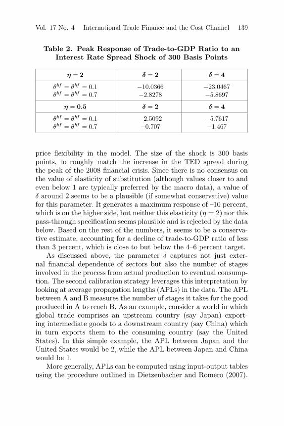
Table 2. Peak Response of Trade-to-GDP Ratio to anInterest Rate Spread Shock of 300 Basis Points
η = 2 δ = 2 δ = 4
θhf = θhf = 0.1 −10.0366 −23.0467θhf = θhf = 0.7 −2.8278 −5.8697
η = 0.5 δ = 2 δ = 4
θhf = θhf = 0.1 −2.5092 −5.7617θhf = θhf = 0.7 −0.707 −1.467
price flexibility in the model. The size of the shock is 300 basispoints, to roughly match the increase in the TED spread duringthe peak of the 2008 financial crisis. Since there is no consensus onthe value of elasticity of substitution (although values closer to andeven below 1 are typically preferred by the macro data), a value ofδ around 2 seems to be a plausible (if somewhat conservative) valuefor this parameter. It generates a maximum response of –10 percent,which is on the higher side, but neither this elasticity (η = 2) nor thispass-through specification seems plausible and is rejected by the databelow. Based on the rest of the numbers, it seems to be a conserva-tive estimate, accounting for a decline of trade-to-GDP ratio of lessthan 3 percent, which is close to but below the 4–6 percent target.
As discussed above, the parameter δ captures not just exter-nal financial dependence of sectors but also the number of stagesinvolved in the process from actual production to eventual consump-tion. The second calibration strategy leverages this interpretation bylooking at average propagation lengths (APLs) in the data. The APLbetween A and B measures the number of stages it takes for the goodproduced in A to reach B. As an example, consider a world in whichglobal trade comprises an upstream country (say Japan) export-ing intermediate goods to a downstream country (say China) whichin turn exports them to the consuming country (say the UnitedStates). In this simple example, the APL between Japan and theUnited States would be 2, while the APL between Japan and Chinawould be 1.
More generally, APLs can be computed using input-output tablesusing the procedure outlined in Dietzenbacher and Romero (2007).

140 International Journal of Central Banking October 2021
Table 3. Average Propagation Length: SummaryStatistics for Benchmark Year 2007
A. Average Propagation Length (APL) Summary Statistics
Country-Level APL Country-Sector-Level APL
No. of Countries 41 No. of Country-Sectors 1,435Mean APL 2.8465 Mean APL 3.61Median APL 2.7396 Median APL 3.62Std. Dev. 0.5 Std. Dev. 0.9
B. APL for Select Country Pairs
United States Germany China
United States 1.70 2.85 3.65Germany 2.83 1.62 3.54China 3.42 3.53 2.48
Source: World Input Output Database (http://www.wiod.org) and authorcalculations.
Table 3 displays summary statistics for APLs computed at the coun-try and country-sector level using detailed intercountry input-outputdata from the World Input-Output Database for the benchmark year2007.34 While the country-level APLs are likely to be biased down-wards since they ignore within-country flows and the heterogeneityis substantial, the values in the range 2 to 5 seem to be reasonablebased on these statistics, which are also in line with the range ofplausible values obtained using the behavior of trade-to-GDP ratios.
4.2 Model Simulations
Figure 1 shows the impulse response of key macroeconomic vari-ables to a contractionary monetary policy shock (in the form of a 25basis point increase in the nominal interest rate) in different versionsof the model.35 These versions differ only along one dimension—the
34See Timmer and Erumban (2012) for a detailed description of the databaseand Dietzenbacher and Romero (2007) for a detailed discussion of APL.
35The contractionary monetary shock corresponds to a surprise increase in thenominal interest rate due to a positive shock to εh
rt in equation (30). The instan-taneous response of the nominal interest rate is less than 25 basis points (the size

Vol. 17 No. 4 International Trade Finance and the Cost Channel 141
Figure 1. Impulse Response to a Home MonetaryContraction: θfh = 0.7, θhf = 0.7
Notes: The impulse responses to a positive 25 basis point shock to the nomi-nal interest rate are computed through simulations using the values in table 1.The horizontal axis measures time in quarters. The vertical axis units are devi-ations from the unshocked path. Inflation and nominal interest rate are given inannualized percentage points. The other variables are in percentages.
interest rate relevant for trade finance. The blue (dashed) lines corre-spond to the specification where all borrowing costs related to inter-national trade finance are linked to the home policy rate, whereas the
of the shock), due to the endogenous response of the nominal interest rate to theshock via the interest rate rule (see, for instance, Galı 2009, chapter 3).

142 International Journal of Central Banking October 2021
green (solid) lines denote the opposite scenario in which borrowingcosts are linked to the policy rate of the foreign economy. For com-parison, red (solid with dots) lines corresponding to a model withouttrade finance are also shown.36 The two economies are assumed to besymmetric in all dimensions, including the degree of price stickinessin the import sector (θfh = 0.7, θhf = 0.7).
Compared with the model without trade finance, the modelin which trade finance is tied to home monetary conditions dis-plays a sharp fall in trade, as captured by the decline in trade-to-GDP ratio (blue dashed line).37 This is a direct consequence oftrade becoming more expensive due to a rise in borrowing coststhat are linked to the home nominal interest rate. Interestingly,however, the response of both home and foreign GDP is virtuallyidentical under the different models. This reflects the confluenceof two effects brought about by the introduction of trade financewhich offset one another. As trade becomes more expensive, con-sumers shift away from imports and towards domestically producedgoods. While the former leads to a fall in aggregate demand dueto a decline in demand for exports, the latter leads to a rise inaggregate demand due to increased demand for domestically pro-duced goods by consumers in each country as they shift consump-tion away from imports. On net, these two effects offset each other,such that the impact of trade finance on the response of GDP tomonetary shocks remains muted in both the home and the foreigneconomy.
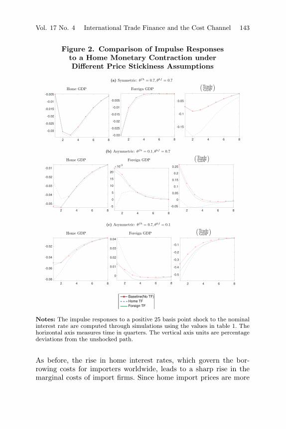
As shown in figure 2, the symmetry across the two countries isimportant for this lack of impact of trade finance on GDP. Panel Ashows the response of GDP and trade under symmetric price stick-iness across countries (θfh = 0.7, θhf = 0.7), the same as in figure1. Panel B shows how when home import prices are more flex-ible than foreign prices (a feature that is uncovered in the datain the following section), trade finance begins to significantly alterthe impact of home and foreign GDP to home monetary shocks.
36For figures in color, see the online version of the paper, available athttp://www.ijcb.org.
37The trade-to-GDP ratio is defined as the ratio of total trade divided by totalGDP, both measured in nominal terms in a common currency.
Vol. 17 No. 4 International Trade Finance and the Cost Channel 143
Figure 2. Comparison of Impulse Responsesto a Home Monetary Contraction underDifferent Price Stickiness Assumptions
Notes: The impulse responses to a positive 25 basis point shock to the nominalinterest rate are computed through simulations using the values in table 1. Thehorizontal axis measures time in quarters. The vertical axis units are percentagedeviations from the unshocked path.
As before, the rise in home interest rates, which govern the bor-rowing costs for importers worldwide, leads to a sharp rise in themarginal costs of import firms. Since home import prices are more

144 International Journal of Central Banking October 2021
flexible, home importers pass on this rise to consumers in the formof higher import prices to a larger extent than foreign importers,whose retail prices are stickier. The net result is a sharp fall in thedemand for imports in the home economy, which, unlike in the caseof symmetric import price stickiness, is not matched by a corre-sponding fall in demand for home exports coming from the foreigncountry. Therefore, compared with the baseline model without tradefinance, the model with trade finance generates a positive impacton home GDP (which consequently declines by less in responseto the monetary shock) and a larger fall in GDP in the foreigneconomy.
The opposite is true if the price asymmetry is reversed such thatthe foreign retail price of imports is more flexible than home, asin panel C. In this case, in comparison with the baseline modelin response to a home monetary shock, the introduction of tradefinance has a positive impact on home GDP and a negative impacton foreign GDP.
Differences in the degree of price stickiness are just one sourceof asymmetry across countries (albeit an important one for whichthe following sections provide evidence). In principle, asymmetries inother dimensions can also break the offsetting effects that make tradefinance constraints irrelevant as far as GDP is concerned. Panel B infigure 3 shows an example where price stickiness is the same acrosscountries, but they differ in the interest rate that is used to financeinternational trade (panel A, for reference, is the same as in the pre-vious two figures). The blue lines correspond to the model in whichexporters are financially constrained and need to borrow workingcapital at a cost linked to the risk-free rate of the exporting country.In this case, when home interest rates rise as a consequence of themonetary contraction, foreign imports (home exports) become moreexpensive for consumers due to the higher borrowing costs of homeexporters. This is not offset by a corresponding rise in the price ofhome imports, since marginal costs of foreign exporters, which arelinked to the foreign risk-free rate, do not rise. As a result, com-pared with the baseline model without trade finance, home GDPfalls more, and foreign GDP less, in response to a home monetarycontraction. The opposite is true when importers who have workingcapital requirements that need to be financed at borrowing costslinked to their domestic risk-free rate (green lines).

Vol. 17 No. 4 International Trade Finance and the Cost Channel 145
Figure 3. Comparison of Impulse Responsesto a Home Monetary Contraction under
Different Financing Arrangements
Notes: The impulse responses to a positive 25 basis point shock to the nominalinterest rate are computed through simulations using the values in table 1. Theprice stickiness parameters are fixed at θfh = 0.7, θhf = 0.7 across all sets of sim-ulations reported in this figure. The horizontal axis measures time in quarters.The vertical axis units are percentage deviations from the unshocked path.
To summarize, the main insight from simulation results is thatwhen countries are completely symmetric in terms of their pricestickiness and trade financing needs, the introduction of tradefinance matters only as far as trade prices and total trade volumesare concerned, but offsetting effects imply that its impact on theresponse of home and foreign GDP is limited. On the other hand,when countries are asymmetric along any of these dimensions, tradefinance exerts a significant influence on the response of home andforeign GDP to shocks.

146 International Journal of Central Banking October 2021
Figure 4. Home Government Spending Shock
Notes: Impulse response to a positive government spending shock in the homecountry. The vertical axis units are deviations from the unshocked path. Inflationand nominal interest rate are given in annualized percentage points. The othervariables are in percentages.
It is important to emphasize that while the impact is most vis-ible in the case of monetary shocks, to the extent that most othershocks generate an endogenous response of the risk-free rate in theeconomy, the impact of trade finance extends to all other businesscycle shocks. Figure 4, for instance, illustrates this for a positivehome government spending (demand) shock.
Vol. 17 No. 4 International Trade Finance and the Cost Channel 147
Figure 5. Competitive Devaluations and Trade
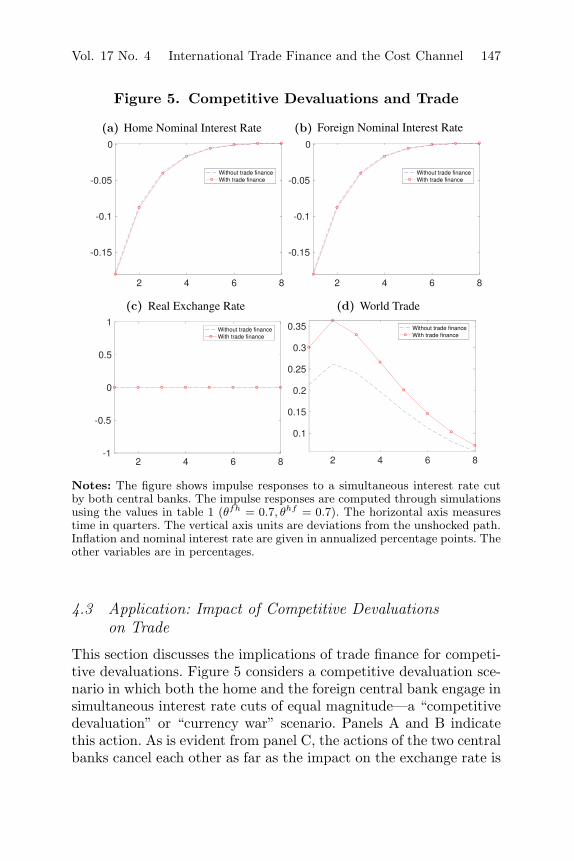
Notes: The figure shows impulse responses to a simultaneous interest rate cutby both central banks. The impulse responses are computed through simulationsusing the values in table 1 (θfh = 0.7, θhf = 0.7). The horizontal axis measurestime in quarters. The vertical axis units are deviations from the unshocked path.Inflation and nominal interest rate are given in annualized percentage points. Theother variables are in percentages.
4.3 Application: Impact of Competitive Devaluationson Trade
This section discusses the implications of trade finance for competi-tive devaluations. Figure 5 considers a competitive devaluation sce-nario in which both the home and the foreign central bank engage insimultaneous interest rate cuts of equal magnitude—a “competitivedevaluation” or “currency war” scenario. Panels A and B indicatethis action. As is evident from panel C, the actions of the two centralbanks cancel each other as far as the impact on the exchange rate is
148 International Journal of Central Banking October 2021
concerned and lead to no change in the real (or nominal) exchangerate. However, as shown in panel D, in a world where trade financeis important, the boost to international trade volumes is much morepronounced. While trade rises in both cases due to the increasedaggregate demand in each country which also spills over into demandfor imports, the fact that the financing constraints on importers andexporters are loosened in a world in which trade finance is presentleads to the much sharper boost in trade. This finding is particu-larly relevant in an environment where trade conflicts are depressingthe outlook for trade. These results show that to the extent thatinternational trade policymakers care about trade over and aboveits impact on contemporaneous output,38 even if devaluations arematched competitively by trade partners, the boost to exports canbe substantially larger than that inferred from models that do notincorporate a role for trade finance.
5. Estimation
As is evident in section 4.2, the role of trade finance in businesscycle fluctuations depends critically on parameters characterizingthe export-import sectors of countries, and in particular on differ-ences across the two countries. This section uses Bayesian techniquesto estimate the model using macroeconomic time-series data fromtwo large open economies—the United States and euro zone.39 Fol-lowing Smets and Wouters (2003) and others, a full-informationlikelihood-based estimation procedure is used.
5.1 Data
The model is matched to the data by treating the United States andeuro zone as the two countries comprising the world economy. Thesample period is 1983:Q1–2007:Q4.40 Table 4 lists the variables used
38One reason why this may be so is because there is an extensive literaturedocumenting the productivity gains from trade—see, for instance, De Loecker(2013).
39See appendix B for a brief description of Bayesian estimation and the modelcomparison exercise.
40Since the subsequent period has been characterized by zero and negativeinterest rates, the monetary policy stance is not well captured by the policy rate.
Vol. 17 No. 4 International Trade Finance and the Cost Channel 149
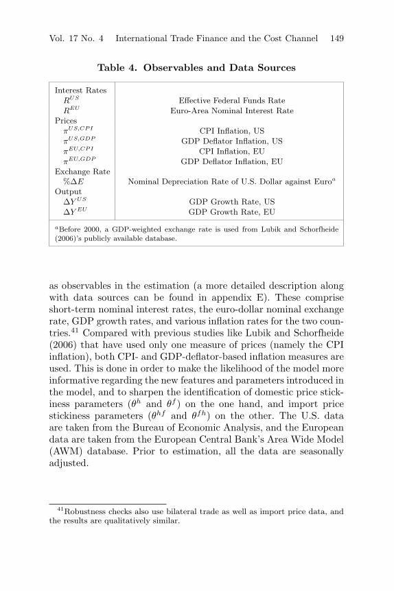
Table 4. Observables and Data Sources
Interest RatesRUS Effective Federal Funds RateREU Euro-Area Nominal Interest Rate
PricesπUS,CPI CPI Inflation, USπUS,GDP GDP Deflator Inflation, USπEU,CPI CPI Inflation, EUπEU,GDP GDP Deflator Inflation, EU
Exchange Rate%ΔE Nominal Depreciation Rate of U.S. Dollar against Euroa
OutputΔY US GDP Growth Rate, USΔY EU GDP Growth Rate, EU
aBefore 2000, a GDP-weighted exchange rate is used from Lubik and Schorfheide(2006)’s publicly available database.
as observables in the estimation (a more detailed description alongwith data sources can be found in appendix E). These compriseshort-term nominal interest rates, the euro-dollar nominal exchangerate, GDP growth rates, and various inflation rates for the two coun-tries.41 Compared with previous studies like Lubik and Schorfheide(2006) that have used only one measure of prices (namely the CPIinflation), both CPI- and GDP-deflator-based inflation measures areused. This is done in order to make the likelihood of the model moreinformative regarding the new features and parameters introduced inthe model, and to sharpen the identification of domestic price stick-iness parameters (θh and θf ) on the one hand, and import pricestickiness parameters (θhf and θfh) on the other. The U.S. dataare taken from the Bureau of Economic Analysis, and the Europeandata are taken from the European Central Bank’s Area Wide Model(AWM) database. Prior to estimation, all the data are seasonallyadjusted.
41Robustness checks also use bilateral trade as well as import price data, andthe results are qualitatively similar.
150 International Journal of Central Banking October 2021
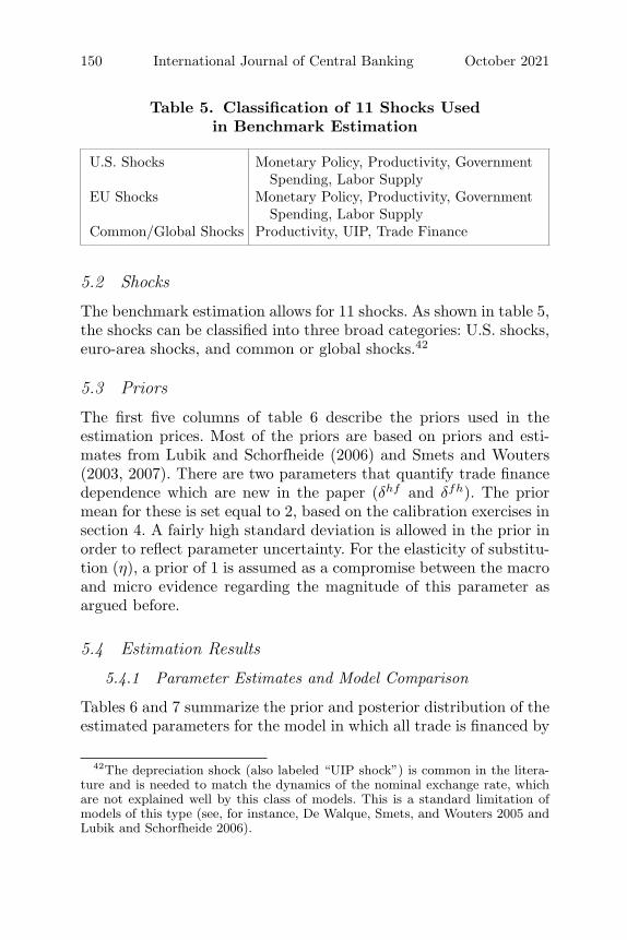
Table 5. Classification of 11 Shocks Usedin Benchmark Estimation
U.S. Shocks Monetary Policy, Productivity, GovernmentSpending, Labor Supply
EU Shocks Monetary Policy, Productivity, GovernmentSpending, Labor Supply
Common/Global Shocks Productivity, UIP, Trade Finance
5.2 Shocks
The benchmark estimation allows for 11 shocks. As shown in table 5,the shocks can be classified into three broad categories: U.S. shocks,euro-area shocks, and common or global shocks.42
5.3 Priors
The first five columns of table 6 describe the priors used in theestimation prices. Most of the priors are based on priors and esti-mates from Lubik and Schorfheide (2006) and Smets and Wouters(2003, 2007). There are two parameters that quantify trade financedependence which are new in the paper (δhf and δfh). The priormean for these is set equal to 2, based on the calibration exercises insection 4. A fairly high standard deviation is allowed in the prior inorder to reflect parameter uncertainty. For the elasticity of substitu-tion (η), a prior of 1 is assumed as a compromise between the macroand micro evidence regarding the magnitude of this parameter asargued before.
5.4 Estimation Results
5.4.1 Parameter Estimates and Model Comparison
Tables 6 and 7 summarize the prior and posterior distribution of theestimated parameters for the model in which all trade is financed by
42The depreciation shock (also labeled “UIP shock”) is common in the litera-ture and is needed to match the dynamics of the nominal exchange rate, whichare not explained well by this class of models. This is a standard limitation ofmodels of this type (see, for instance, De Walque, Smets, and Wouters 2005 andLubik and Schorfheide 2006).

Vol. 17 No. 4 International Trade Finance and the Cost Channel 151
Tab
le6.
Sum
mar
yof
Pri
oran
dPos
teri
orP
rior
and
Pos
teri
orD
istr
ibution
ofEst
imat
edPar
amet
ers
Pri
orPos
teri
or
Par
amet
erD
escr
ipti
onD
istr
ibuti
onM
ean
Std
.D
ev.
Mea
n90
%C
.I.
θU
SC
alvo
Dom
esti
cB
eta
0.7
0.05
0.83
70.
80.
874
θU
SIm
port
Cal
voIm
port
Bet
a0.
50.
10.
377
0.22
90.
518
θEU
Import
Cal
voIm
port
Bet
a0.
50.
10.
872
0.72
60.
986
θEU
Cal
voD
omes
tic
Bet
a0.
70.
050.
750.
695
0.80
7σ
cIn
tert
empo
ralC
onsu
mpt
ion
Ela
stic
ity
Gam
ma
10.
254.
512
3.30
95.
751
σL
Lab
orSu
pply
Ela
stic
ity
Gam
ma
20.
51.
541
0.96
62.
092
hH
abit
Par
amet
erB
eta
0.5
0.1
0.54
70.
395
0.69
7η
Intr
atem
pora
lE
last
icity
Gam
ma
10.
30.
408
0.25
0.55
8φ
US
πTay
lor-
Rul
ePar
amet
erG
amm
a1.
50.
251.
926
1.59
12.
232
φU
Sy
Tay
lor-
Rul
ePar
amet
erG
amm
a0.
50.
250.
452
0.20
60.
68
φU
Se
Tay
lor-
Rul
ePar
amet
erG
amm
a0.
10.
050.
031
0.01
0.05
1
φE
Uπ
Tay
lor-
Rul
ePar
amet
erG
amm
a1.
50.
251.
862
1.52
42.
219
φE
Uy
Tay
lor-
Rul
ePar
amet
erG
amm
a0.
50.
250.
546
0.24
60.
845
φE
Ue
Tay
lor-
Rul
ePar
amet
erG
amm
a0.
10.
050.
030.
008
0.05
ρU
SA
U.S
.T
FP
Per
sist
ence
Bet
a0.
80.
10.
996
0.99
20.
999
ρU
SR
U.S
.In
tere
stR
ate
Smoo
thin
gB
eta
0.5
0.2
0.82
10.
789
0.85
6
ρU
SG
U.S
.G
over
nmen
tSp
endi
ngPer
sist
ence
Bet
a0.
80.
10.
963
0.94
10.
985
ρE
UA
EU
TFP
Per
sist
ence
Bet
a0.
60.
20.
574
0.25
90.
906
ρE
UR
EU
Inte
rest
Rat
eSm
ooth
ing
Bet
a0.
50.
20.
867
0.84
30.
892
ρE
UG
EU
Gov
ernm
ent
Spen
ding
Per
sist
ence
Bet
a0.
80.
10.
930.
891
0.97
1ρ
ZG
loba
lP
rodu
ctiv
ity
Per
sist
ence
Bet
a0.
660.
150.
461
0.25
80.
661
δEU
→U
STra
deFin
ance
Par
amet
er:U
SG
amm
a2
0.75
2.27
0.99
13.
423
δUS
→E
UTra
deFin
ance
Par
amet
er:U
SG
amm
a2
0.75
1.83
70.
735
2.90
9ρ
US
NU
.S.Lab
orSu
pply
Shoc
kPer
sist
ence
Bet
a0.
850.
10.
810.
743
0.87
8
ρE
UN
EU
Lab
orSu
pply
Shoc
kPer
sist
ence
Bet
a0.
850.
10.
894
0.84
90.
939
Note
s:T
here
sult
sar
eba
sed
on20
0,00
0M
CM
Cdr
aws
(spl
itac
ross
two
chai
ns)
afte
rbu
rn-in
wit
hth
epos
teri
orm
ode
used
asth
est
arti
ngva
lue
for
each
para
met
er.T
helis
tof
obse
rvab
les
isgi
ven
inta
ble
4.

152 International Journal of Central Banking October 2021
Table 7. Summary of Priors and Posterior Distributionsof Standard Deviations of Shocks
Prior Std. PosteriorShock Distribution Mean Dev. Mean 90% C.I.
Ah Invg. 1.253 0.655 1.167 0.873 1.463Gh Invg. 1.253 0.655 0.526 0.451 0.6Rh Invg. 0.501 0.262 0.161 0.139 0.183Af Invg. 0.501 0.262 0.464 0.224 0.707Gf Invg. 1.253 0.655 0.502 0.432 0.569Rf Invg. 0.251 0.131 0.138 0.12 0.156Z Invg. 0.627 0.328 0.337 0.236 0.434ΔE Invg. 4.387 2.293 4.166 3.673 4.643Nh Invg. 0.101 0.262 1.563 1.355 1.755Nf Invg. 2 0.5 2.608 1.722 3.472
Notes: “Invg.” denotes the inverse gamma distribution. The last two rows corre-spond to measurement errors of the corresponding observed variables. h denotes thehome country (United States) and f denotes the foreign country (European Union).
borrowing at the U.S. interest rate. (This is the model that is mostpreferred by the data, i.e., has the highest Bayes factor, as will bediscussed later.)
The posterior estimates of the price stickiness parameters implythat the data support a model in which there is asymmetry in thepass-through into import prices across the two countries. While thepass-through into EU import prices is quite low (θEU Import hasa posterior mean of 0.87), the corresponding value for the UnitedStates is fairly high (posterior mean of θUS Import is 0.38).
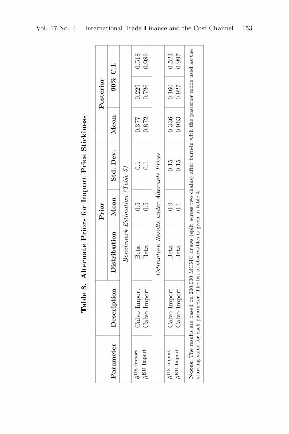
Given the importance of the import price stickiness parameters indriving the results of the model, table 8 reports additional robust-ness checks on the estimated values. It imposes priors that implyexactly the opposite price stickiness pattern to the one estimatedin the data (table 6), and finds that the results are robust to thischange in the priors.
These results are in line with estimates from Lubik andSchorfheide (2006), who also find evidence in favor of this asym-metry. Table 9 shows a comparison of the posterior means for theCalvo parameters from table 6. In their case this difference may also
Vol. 17 No. 4 International Trade Finance and the Cost Channel 153
Tab
le8.
Alter
nat
eP
rior
sfo
rIm
por
tP
rice
Stick
ines
s
Pri
orPos
teri
or
Par
amet
erD
escr
ipti
onD
istr
ibuti
onM
ean
Std
.D
ev.
Mea
n90
%C
.I.
Ben
chm
ark
Est
imat
ion
(Tab
le6)
θUS
Impor
tC
alvo
Impo
rtB
eta
0.5
0.1
0.37
70.
229
0.51
8θE
UIm
por
tC
alvo
Impo
rtB
eta
0.5
0.1
0.87
20.
726
0.98
6
Est
imat
ion
Res
ults
unde
rA
ltern
ate
Pri
ces
θUS
Impor
tC
alvo
Impo
rtB
eta
0.9
0.15
0.33
60.
160
0.52
3θE
UIm
por
tC
alvo
Impo
rtB
eta
0.1
0.15
0.96
30.
927
0.99
7
Note
s:T
here
sult
sar
eba
sed
on20
0,00
0M
CM
Cdr
aws
(spl
itac
ross
two
chai
ns)
afte
rbu
rn-in
wit
hth
epos
teri
orm
ode
used
asth
est
arti
ngva
lue
for
each
para
met
er.T
helis
tof
obse
rvab
les
isgi
ven
inta
ble
4.

154 International Journal of Central Banking October 2021
Table 9. Comparison of Calvo Parameters withLubik and Schorfheide (2006)
Lubik and Schorfheide (2006)
Posterior Posterior 90% PriorMean Mean C.I. Month
θUS 0.83 0.62 [0.49, 0.77] 0.5θUS Import 0.38 0.45 [0.17, 0.72] 0.5θEU Import 0.87 0.9 [0.82, 1.00] 0.75θEU 0.75 0.61 [0.43, 0.81] 0.75
be partly driven by the choice of their prior distribution, which isasymmetric and implies higher price flexibility in the United Statesthan in the EU for both domestic and import prices.43 This paperon the other hand does not impose this asymmetry ex ante.
Notwithstanding the fact that the estimates of the price stick-iness parameters are in line with the estimates of Lubik andSchorfheide (2006), at first sight they seem to be at odds with theextensive literature on pass-through into import prices which hasfound the pass-through (in particular, with regard to the nomi-nal exchange rate) into U.S. import prices to be low, pointing toa very low import price flexibility for the United States.44 Althougha thorough exploration of this apparent discrepancy would requiredetailed examination of micro data and is beyond the scope of thispaper, two possible explanations can be conjectured. Firstly, whilethe trade literature has focused for the most part on exchange ratepass-through, the asymmetry revealed here is with regard to pass-through of marginal costs into prices more generally, including othercomponents of marginal costs apart from the nominal exchange rate.Secondly, while the trade literature has focused on import prices atthe dock, the estimates in the model correspond to the retail priceof imports. Understanding the journey of imports from the dock toeventual retail outlets, including the characteristics of the different
43They rely on Angeloni et al. (2006) and Bils and Klenow (2004) to impose ahigh prior mean for Europe and a lower one for the United States.
44See, for instance, Gopinath, Itskhoki, and Rigobon (2010).

Vol. 17 No. 4 International Trade Finance and the Cost Channel 155
markets and intermediaries involved, would be an important part ofinterpreting these findings.
With regard to δ, the other parameter which governs the strengthof the trade finance channel, table 6 shows that the posterior meansare 2.27 and 1.87 for δEU→US and δUS→EU , respectively. These arebroadly in line with the calibrated values used in section 4.45
In terms of the reduced-form interpretation of equation (25), thisestimate implies that the elasticity of the trade finance rate withrespect to the risk-free rate is around 2, implying that a 1 percent-age point increase in the risk-free rate leads to about a 2 percentagepoint increase in the total cost of trade finance. While the mag-nitudes are again roughly consistent with the average propagationlengths estimates in the data, the 90 percent interval includes val-ues high enough to imply an inferred external finance dependencegreater than 1. This suggests that there remains scope for alternativemicrofoundations of the parameter δ.
Table 10 reports the log marginal density for various specifica-tions of the model that are estimated, along with the Bayes factorfor each model in comparison with the model without trade finance.Assuming the prior probabilities to be the same across models,numbers in each column (i.e., estimates based on the same num-ber of observables) can be interpreted as measures of the posteriorodds ratios, with higher numbers (lower absolute values) indicatinghigher posterior odds for the corresponding model.46 The last col-umn reports Bayes factors computed with respect to the baselinemodel with no trade finance, which by construction has a Bayes fac-tor of 1 with respect to itself. Bayes factors greater than 1 indicatethat the respective model is more preferred by the data than thebaseline model. According to Jeffreys (1998), a Bayes factor greaterthan 30 is “very strong ” and a Bayes factor greater than 20 is“decisive” evidence.
The table shows that the models with trade financing with U.S.interest rates and importer interest rates carry the highest posteriorprobability and Bayes factors. The first of these is not surprising,
45Given the importance of the δ and θ parameters, appendix C presents someadditional robustness checks on the estimates.
46Note that this comparison is valid as long as the prior is proper, which is thecase throughout this paper.

156 International Journal of Central Banking October 2021
Table 10. Marginal Likelihood for Different Models
Marginal Bayes Factor wrtModel Data Density No Trade Finance
1 No Trade Finance −1236.04 12 Trade Finance: Both
Interest Rates−1233.71 10
3 U.S. Interest RateTrade Finance
−1227.37 5,825
4 EU Interest RateTrade Finance
−1236.15 0.9
5 Importer Interest RateTrade Finance
−1227.42 5,541
6 Exporter Interest RateTrade Finance
−1232.34 40
Note: The second model, “Trade Finance: Both Interest Rates,” allows for tradefinance to be dependent on both home and foreign interest rates.
given the central role that U.S. monetary policy plays in the globaleconomy and given the fact that the dollar is also the primary vehi-cle currency in which international trade is conducted.47 The higherposterior marginal data density of the model with importer interestrate trade finance on the other hand is less easier to motivate, giventhat the majority of the empirical literature in trade finance hasdocumented the link between exporter monetary policy and volumeof exports. However, a close examination of the arguments given forthese apply equally to the link between imports and interest ratesas well. In fact, in his empirical analysis Schmidt-Eisenlohr (2013)finds the role of importer interest rate to be as important as theexporter one.
What these results indicate in conjunction is that in the data,the trade finance channel seems to be governed by the interaction ofU.S. interest rates with U.S. imports. Since European imports playa limited role due to their low price flexibility, the models with U.S.interest rate and importer interest rate financing both seem to beconsistent, and the data are not clearly able to distinguish betweenthe two.
47For evidence regarding the latter, see Goldberg and Tille (2008).
Vol. 17 No. 4 International Trade Finance and the Cost Channel 157
5.4.2 Variance Decompositions48
The simulation results in section 4 show that incorporation of tradefinance has a disproportionately large effect on the spillover effectsof shocks, as opposed to the effect on the domestic economy. Thisraises a queston of how much the proposed model fundamentallychanges our understanding of the importance of U.S. shocks for euro-area business cycles. Table 11 provides a comparison of the variancedecomposition of euro-area variables at two horizons for two cate-gories of shocks according to the classification in table 5—domesticU.S. shocks and all external shocks which include U.S. shocks andthe global shocks in table 5. The numbers in the table denote thedifference between the share (out of 1) of the variance of the row vari-able explained by the model with trade finance and the one without.Positive numbers therefore convey that U.S. and external shocks aremore important in the model with trade finance for the particularvariable, whereas negative numbers indicate the opposite.49
The differences in the long-run variance decomposition (horizon =∞) are unanimous in suggesting that ignoring trade finance overstatesthe importance ofU.S. shocks aswell as external shocksmore generallyfor the euro area. Indeed, the differences are negative for all the euro-areavariables.Theresultsare lessclear-cut inthecaseof short-runvari-ance decompositions (horizon = one quarter), where the model withtradefinancedoesgiveahigherweight to external shocks formost euro-area quantity variables such as output, consumption, and imports,but not to price variables such as inflation and the real exchange rate.
To summarize, the model with trade finance suggests that whileexternal shocks are more important in explaining the short-runvariance of some variables such as output and consumption, over-all, external shocks including U.S. domestic shocks are much less
48Appendix D provides additional comparisons between the model with andwithout trade finance based on posterior predictive moments.
49For example, the number corresponding to the row “Imported Inflation” andcolumn “Domestic U.S. Shocks” under the “Horizon = ∞” panel shows that foreuro-area imported inflation, domestic U.S. shocks account for 0.46 (out of 1)more variance according to the model without trade finance, compared with theone with trade finance, i.e., for example, if in the model without trade finance,U.S. shocks account for 0.8 (or 80 percent) of the variance of euro-area importinflation, they account for only only 0.34 (or 34 percent) of the variance in themodel with trade finance.

158 International Journal of Central Banking October 2021
Tab
le11
.V
aria
nce
Dec
ompos
itio
nfo
rEuro
Are
a:D
iffer
ence
bet
wee
nM
odel
sw
ith
and
withou
tTra
de
Fin
ance
Dom
esti
cU
.S.
All
Exte
rnal
Dom
esti
cU
.S.
All
Exte
rnal
Shock
sShock
sShock
sShock
s
Var
iable
(Euro
Are
a)H
oriz
on=
∞H
oriz
on=
1
GD
P−
0.00
1−
0.00
10.
000.
114
Infla
tion
−0.
006
−0.
478
−0.
003
−0.
161
Impo
rted
Infla
tion
−0.
009
−0.
416
−0.
008
−0.
12C
onsu
mpt
ion
−0.
006
−0.
006
−0.
019
0.40
8N
omin
alIn
tere
stR
ate
−0.
037
−0.
046
−0.
004
−0.
004
Impo
rts
−0.
459
−0.
456
−0.
562
0.14
1E
xpor
ts−
0.01
7−
0.01
8−
0.11
5−
0.00
9Ter
ms
ofTra
de−
0.1
−0.
1−
0.19
6−
0.19
Rea
lE
xcha
nge
Rat
e−
0.11
−0.
114
−0.
232
−0.
36N
omin
alD
epre
ciat
ion
−0.
013
−0.
11−
0.01
6−
0.09
5
Note
s:T
henu
mber
sin
the
tabl
ede
note
the
differ
ence
bet
wee
nth
esh
are
ofth
eva
rian
ceof
the
row
vari
able
expl
aine
dby
the
mod
elw
ith
trad
efin
ance
and
the
one
wit
hout
.Pos
itiv
enu
mber
sth
eref
ore
conv
eyth
atth
em
odel
wit
htr
ade
finan
ceex
plai
nsa
high
ersh
are
ofth
eva
rian
ceof
the
vari
able
,w
here
asne
gati
venu
mber
sin
dica
teth
eop
pos
ite.

Vol. 17 No. 4 International Trade Finance and the Cost Channel 159
important for euro-area business cycles. This is an important take-away for policymakers, as the role of external versus domestic shocksin driving business cycle fluctuations has different implications fortheir policy frameworks.
5.4.3 Comparison to an Atheoretical Benchmark: DSGE-VAR
This section uses the DSGE-VAR approach to assess the fit of themodel with respect to an atheoretical benchmark—an unrestrictedVAR.50
The approach exploits the fact that estimating a DSGE modelis akin to estimating a VAR with cross-equation restrictions, andallows for the extent to which the restrictions can be imposed orrelaxed. In particular, there is a hyperparameter λ ≥ 0 such that theDSGE model restrictions are strictly imposed if λ = ∞, whereas therestrictions are completely ignored if λ = 0. Estimation of the VARuses a prior that is centered at the DSGE-model-implied restrictions.The hyperparameter λ scales the covariance matrix of the prior. Ifit is large, most of the variance is centered around the DSGE model.The prior is combined with the likelihood to obtain the posteriorof λ.51
Table 12 summarizes the estimation results for λ. The fact thatthe posterior of λ shifts towards zero compared with the prior indi-cates that some of the restrictions in the model are at odds withthe data. This is in line with the results obtained in Lubik andSchorfheide (2006) and Smets and Wouters (2003), and highlightsthat estimated DSGE models are typically worse than some VARspecifications. That said, the posterior of λ, as well as the marginallikelihood, is higher in the case of the model with trade financethan without. This suggests that even when evaluated against anatheoretical benchmark like an unconditional VAR, the model withtrade finance continues to provide a better fit to the data, and thedata relaxes less of its cross-equation restrictions compared with themodel that lacks a role for trade finance.
50For a detailed description of the procedure see, for instance, Del Negro et al.(2007) and Del Negro and Schorfheide (2004, 2006).
51The parameters of the DSGE model are also estimated simultaneously inthe procedure by projecting the parameters of the estimated VAR back onto theDSGE parameter space.
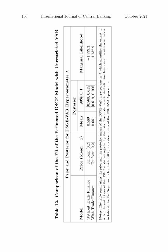
160 International Journal of Central Banking October 2021
Tab
le12
.C
ompar
ison
ofth
eFit
ofth
eEst
imat
edD
SG
EM
odel
with
Unre
stri
cted
VA
R
Pri
oran
dPos
teri
orfo
rD
SG
E-V
AR
Hyper
par
amet
erλ
Pos
teri
or
Model
Pri
or(M
ean
=1)
Mea
n90
%C
.I.
Mar
ginal
Lik
elih
ood
Wit
hout
Tra
deFin
ance
Uni
form
[0,2
]0.
589
[0.5
60,0.
615]
−1,
799.
3W
ith
Tra
deFin
ance
Uni
form
[0,2
]0.
661
[0.6
19,0.
706]
−1,
732.
9
Note
s:T
heta
ble
sum
mar
izes
the
prio
ran
dth
epos
teri
orm
eans
ofth
eD
SGE
-VA
Rhy
per
para
met
erλ
whi
chqu
anti
fies
the
exte
ntto
whi
chth
ere
stri
ctio
nsof
the
DSG
Em
odel
are
reje
cted
byth
eda
ta.T
hem
odel
ises
tim
ated
wit
hfo
urla
gsus
ing
the
nine
obse
rvab
les
inta
ble
4.Se
eD
elN
egro
and
Scho
rfhe
ide
(200
6)fo
ra
desc
ript
ion
ofth
eD
SGE
-VA
Rpr
oced
ure.

Vol. 17 No. 4 International Trade Finance and the Cost Channel 161
Figure 6. U.S. Monetary Contraction
Note: Baseline model (dotted line) assumes U.S. interest rate trade finance.
5.4.4 Comparison of Shock Propagation Mechanism acrossEstimated Versions of the Model
This section illustrates the differences in propagation mechanismsusing estimated impulse responses from the model. Figure 6 showsthe impulse response of a one-standard-deviation U.S. monetarycontraction (median and 90 percent confidence bands) using theestimated model with U.S. trade finance (the model with thehigher posterior probability than the standard model). For com-parison, the figure also shows two impulse responses correspondingto the standard model. One of these (labeled “Estimated w/o Trade

162 International Journal of Central Banking October 2021
Finance (Median)”) corresponds to the estimated model withouttrade finance constraints, and the second (labeled “Simulated w/oTrade Finance”) corresponds to the impulse response from the sim-ulated model with all parameters at the posterior mean from themodel with trade finance constraints except the trade finance depen-dence parameters themselves, which are set to zero. These are twoalternate ways of comparing the results with the estimated modelwith trade finance. Qualitatively, the results in figure 6 are broadlyin line with the simulation results. Quantitatively, the figure showsthat while the models generate similar predications for the responseof domestic GDP, they differ appreciably in the response of foreignGDP and terms of trade.
One implication of this is that for a large open economy like theUnited States whose business cycle fluctuations are mostly driven bydomestic shocks, excluding trade finance from models might be aninnocuous omission. On the other hand, if the object of interest is tostudy spillover effects from foreign shocks (as would typically be thecase for a small open economy), ignoring trade finance constraintscan lead to severe misrepresentation of the important transmissionchannels in the model. This is due to the fact that trade financeexerts its influence on shock propagation by affecting terms of trade,which translates into changes in trade volumes. As far as the domes-tic economy is concerned, it is therefore best seen as an additionalchannel, while the main effects of the shock are likely to come fromthe direct domestic impact of shock. On the other hand, as far as theforeign economy and spillover effects are concerned, the entire effectof the domestic shock is transmitted through the external sector,which in turn is affected by trade finance. As a result, incorpora-tion of trade finance matters more for spillover effects of shocks asopposed to domestic effects.
6. Conclusion
An extensive literature in international trade has documented theheavy reliance of international trade flows on external finance andhas shown that external financing matters more for internationaltrade as opposed to intranational trade. This paper assesses how thisfeature affects aggregate business cycle fluctuations and the trans-mission mechanism of monetary policy. It does so by modeling the

Vol. 17 No. 4 International Trade Finance and the Cost Channel 163
link between trade finance and the cost channel of monetary pol-icy in a two-country New Keynesian model. Unlike the domesticcomponent of the cost channel of monetary policy which has beenstudied extensively in the literature, the paper shows that the costchannel when combined with trade finance has much richer implica-tions for business cycles, both qualitatively and quantitatively. Morespecifically, it shows that when external sectors are symmetric acrosscountries, trade finance constraints lead to sharp movements in tradeprices and volumes, but do not significantly alter the response ofGDP to shocks in either the home country or abroad, due to offset-ting effects. On the other hand, if external sectors are asymmetric,trade finance constraints significantly change the response of GDP toboth monetary and nonmonetary shocks. The paper identifies vari-ous sources of such asymmetry (including differences in import priceflexibility) and studies their implications. The parameter estimatesprovide compelling evidence for asymmetry in import price flexibil-ity across the two countries. In particular, U.S. retail import pricesare found to be more flexible than their European counterpart.
Using Bayesian techniques, the paper estimates a two-countryDSGE model with macroeconomic time-series data from the UnitedStates and the euro zone, two regions which share one of the largestbilateral trade relationships in the world. Based on model compar-ison exercises, models that appropriately incorporate trade financeconstraints are shown to be preferred by the data. Furthermore,trade finance is found to have a larger impact on spillover effects ofshocks rather than the effects on the country of origin. For example,euro-zone output contracts sharply in response to U.S. monetarycontractions once the model is allowed to appropriately account forthe trade finance channel, while the impact is indistinguishable fromzero in the model without trade finance. In addition, appropriatelyaccounting for trade finance in the model significantly reduces theimportance of external (including domestic U.S.) shocks for euro-area business cycles. This is an important takeaway for policymak-ers, as the role of external versus domestic shocks in driving businesscycle fluctuations has different implications for their policy frame-works. These results also carry important implications for the theoryof competitive devaluations. By relaxing financing constraints onexporters and importers worldwide, devaluations are likely to boosttrade volumes even more strongly than inferred by standard models.

164 International Journal of Central Banking October 2021
An important limitation of this paper that future research war-rants addressing is with respect to the rigidity in modeling the choiceof trade finance by firms. Firms in the model are not allowed toswitch between sources of funding in response to shocks. While thisassumption is well grounded in the large body of empirical workdocumenting the stickiness in firms’ funding sources (Degryse et al.2019, Jimenez et al. 2012, and Khwaja and Mian 2008), and may bejustifiable for the sample period considered in the paper which coin-cides with the great moderation period when the shocks hitting theeconomy were not too large, an extension of the model to endoge-nize firms’ funding choices is bound to provide a more comprehensiveunderstanding of the role of trade finance for business cycle fluctua-tions.52 If firms could switch instantaneously, completely, and cost-lessly from one funding source to another, then the impact of tradefinance on business cycles could be mitigated. The mitigation wouldbe particularly pronounced, and may even lead to a rise in trade, ifthe interest rates of the two countries move in opposite directionsin response to a shock, since in that case exporters and importerswould benefit from a decrease in the cost of financing by switchingto the lower interest rate. The fact that the data overwhelminglyfind a role for trade finance is indicative that while firms may switchbetween funding sources, it may not be reasonable to assume thatthis switch is instantaneous and costless.
Appendix A. Model with Sticky Wages
The household problem is to maximize utility given by
max∞∑
j=0
(βθhw)jEt(Ut+j(Ct+j , Ht+j , Nt+j(h)) (A.1)
subject to the per-period budget constraint given by
P ,cpit Ct +
∫s
μt,t+1(s)Dt+1(s) ≤ WtNt + Dt + Tt (A.2)
52Indeed, recent empirical work looking specifically at exporting firms hasfound that many of them do in fact switch sources of funding in response toshocks—see, for instance, Antras and Foley (2015), Demir and Javorcik (2018)and Garcia-Marin, Justel, and Schmidt-Eisenlohr (2019).

Vol. 17 No. 4 International Trade Finance and the Cost Channel 165
and the labor demand schedule given by
Nt(j) =(
Wt(j)Wh
t
)−η
Nt∀t. (A.3)
Here (1 − θw) denotes the time-invariant probability ofre-adjusting wages in a given period.
The first-order condition implies the following expression for thewage negotiated by households who optimize in a given period:
W ∗t =
∑j(βθw)jEt (Nt+j(h)UN (t + j))∑
j(βθw)jEt
(Nt+j(h)UC(t + j)
(η−1
η
)1
pc,t+j
) , (A.4)
which linearizes to
w∗t = (βθw)Et( ˆw∗
t+1) + (1 − βθw)(UN (t) − Uc(t) + pc(t)
). (A.5)
The aggregate wage evolves according to the following equation:
wt = (1 − θw)w∗t + θwwt−1. (A.6)
Combining (A.5) and (A.6), we can write the Phillips-curve ana-logue of real wage inflation as follows:
wt =βθw
1 + βθ2w
Etwt+1 +θw
1 + βθ2w
wt−1
+(1 − βθw)(1 − θw)
1 + βθ2w
(UN (t) − Uc(t) + pc(t)).
Appendix B. Bayesian Estimation Preliminaries
Let M denote a generic model and let θM be the vector of para-meters associated with it. Let Y denote the data that is used toestimate the model (note that Y does not have an M subscript, i.e.,it is assumed that the data used is the estimation routine is constantacross models). Bayesian estimation proceeds by specifying a priordistribution over θM which is denoted here by P(M, θM). The prior isthen combined with the likelihood computed using the data to formthe posterior distribution of parameters as follows:
P(θM|M, Y) ∝ P(Y|M, θM)P(M, θM). (B.1)

166 International Journal of Central Banking October 2021
Draws from the posterior distribution are generated by apply-ing the Gibbs sampler using standard Markov chain Monte Carlo(MCMC) techniques.53
B.1 Model Selection
The marginal density of the data given the model M is given by
P(Y|M) =∫
θM
P(Y|M, θM)P(M, θM). (B.2)
This quantity has the interpretation of being the probability ofobserving the data given the true model is M. In order to com-pare two models M1 and M2, first the prior odds are specified forboth models. These are then combined with the marginal densitiesto obtain posterior odds ratios which are used for the purpose ofmodel comparison.
PO1|2 =P(Y|M1)P(M1)P(Y|M2)P(M2)
(B.3)
One advantage of the Bayesian framework is that the models donot have to be nested.54 Throughout this paper, a non-informativeprior is assumed on the models (P(M1) = P(M2) = 0.5) so that theratio of marginal data densities is equal to the posterior odds ratio,which in this case is also equal to the frequently quoted statisticcalled the Bayes factor.
Appendix C. Bayesian Estimation Robustness Checks
The parameters quantifying import price flexibility as well as theelasticity of marginal cost with respect to the risk-free rate are crit-ical in determining the role played by trade finance in propagationof business cycle shocks. This section conducts a series of robustnesschecks with regard to these parameters. Table C.1 reports posterior
53See Koop, Poirier, and Tobias (2007) for an overview of MCMC techniques.54Note however that in order for the data densities to be comparable, the data
used in estimating the two models should be the same and the priors should beproper (i.e., they should define a valid distribution that integrates to one). Theseconditions will be imposed throughout the paper in order to keep the modelcomparisons valid.

Vol. 17 No. 4 International Trade Finance and the Cost Channel 167
Table C.1. Posterior Means of Key Parameters underDifferent Model Assumptions/Restrictions
θUS Import θEU Import δEU→US δUS→EU
σc = 1 0.31 0.72 2.02 1.68η = 1 0.33 0.96 2.40 1.94Domestic Cost
Channel 0.33 0.84 2.36 1.89Sticky Wages 0.37 0.84 2.12 1.79
Note: The prior mean and standard deviation of the parameters is the same as thatin the benchmark case (table 6) except when indicated in the first column.
means of these parameters under different variations of the model.For each of the cases reported in table C.1, the prior mean andstandard deviation of the parameters is the same as that in thebenchmark case (table 6) except when indicated in the first column.
Since the elasticity of intertemporal substitution is estimated tobe somewhat higher in comparison with the literature in the baselinecase, the first row considers a model with log utility. The second rowconsiders another restriction on the model by fixing the intratem-poral elasticity of substitution between domestic and foreign bun-dles. As argued before, there is little consensus in the value of thisparameter in the literature, and a value of 1 can be considered acompromise between the trade and business cycle literatures.55 Thethird row considers a model in which the cost channel of monetarypolicy is operational even in the domestic sector, i.e., even the goods-producing firms are required to borrow in order to finance their wagebill. This is typically how the cost channel of monetary policy hasbeen modeled in the literature so far.56 As is evident from the resultsreported in the table, the estimates of the main parameters of inter-est are robust to all these departures from the baseline version ofthe model.
55A more thorough approach would be to allow for dynamic elasticities asdiscussed in Crucini and Davis (2013) and Drozd, Kolbin, and Nosal (2014).However, this approach is not undertaken since the main message of the paper isrobust to the value of the elasticity used.
56See, for instance, Barth and Ramey (2002), Christiano, Eichenbaum, andEvans (2005), and Ravina (2007).

168 International Journal of Central Banking October 2021
Table D.1. Comparison of Data- andModel-Generated Variances
Model with Model withoutData Trade Finance Trade Finance
1 πUS,CPI 1.55 0.85 1.22 πEU,CPI 2.78 4.92 2.755 ΔY US 0.31 0.39 0.46 ΔY EU 0.22 0.34 0.317 %ΔE 19.99 18.58 21.42
Appendix D. Posterior Predictive Moments
The estimation results in the main text show that the model withtrade finance provides a better fit to the data, as measured by themarginal density. To help shed some light on which moments of thedata the two models help match better, this section discusses someof the posterior predictive moments generated by the two modelsand compares them with their counterparts in the data.57 Table D.1presents a comparison of the variances of output and inflation forthe two countries as well as the nominal exchange rate deprecia-tion. While the model with trade finance yields variances for U.S.output and the nominal exchange rate depreciation that are closerto the data, the model without trade finance performs better withrespect to the other variances. The model with trade finance beginsto outperform the model without trade finance more systematicallywhen going to higher order and cross-moments. As an example,table D.2 presents a comparison of the autocorrelations of the differ-ent variables generated by the two models with the data. An entry of“1” indicates that the corresponding value of the model with tradefinance was closer to the data, while “0” indicates that the valuefor the model without trade finance is closer to the correspondingvalue in the data. In total, the model with trade finance generatesmoments that are closer to the data in 42 out of the 72 possibleinstances.
57See An and Schorfheide (2007) for a similar approach.

Vol. 17 No. 4 International Trade Finance and the Cost Channel 169
Tab
leD
.2.
Com
par
ison
ofA
uto
corr
elat
ions
bet
wee
nM
odel
sw
ith
and
withou
tTra
de
Fin
ance
and
the
Dat
a
Lag
s↓π
US
,CP
Iπ
EU
,CP
IR
US
RE
UΔ
YU
SΔ
YE
U%
ΔE
πE
U,G
DP
πU
S,G
DP
10
00
00
10
10
20
10
00
10
11
31
10
00
11
11
41
10
00
11
11
51
10
01
11
01
61
11
01
10
11
71
01
01
11
11
81
01
00
10
01
Note
:“1
”in
dic
ates
that
the
corr
espon
din
gva
lue
ofth
em
odel
wit
htr
ade
finan
cew
ascl
oser
toth
edat
a,w
hile
“0”
indic
ates
that
the
valu
efo
rth
em
odel
wit
hou
ttr
ade
finan
cew
ascl
oser
toth
eco
rres
pon
din
gva
lue
inth
edat
a.

170 International Journal of Central Banking October 2021
Appendix E. Data
E.1 Correlations and Plots
This appendix provides the details and sources for the data usedin the empirical part of the paper. Unless otherwise mentioned, thedata are at quarterly frequency from 1983:Q1–2007:Q4. They areseasonally adjusted and demeaned before estimation.
U.S. Data:
• RUS : Effective federal funds rate, nominal, annualized,percentage
• �Y US : Quarter-to-quarter growth rate of GDP per capitacomputed as follows:
�Y USt = 100
[log
(GDPt
POPt
)− log
(GDPt−1
POPt−1
)]Note: Nominal GDP is converted to real using the GDPdeflator.
• CPI Inflation:
πCPI,USt = 400 [log (CPIt) − log (CPIt−1)]
• GDP Deflator Inflation:
−πGDP,USt = 400 [log (GDPDEFt) − log (GDPDEFt−1)]
• Import Price Inflation (used only in robustness checks, notused in benchmark estimation)
−πIM,USt = 400 [log (PIM,t) − log (PIM,t−1)]
Data Sources: The data for the U.S. block are taken from theBureau of Economic Analysis (BEA) National Income and ProductAccounts (NIPA). The data on population are taken from Ramey(2011)’s publicly available data set.
EU Data:
• REU : Effective federal funds rate, nominal, annualized,percentage

Vol. 17 No. 4 International Trade Finance and the Cost Channel 171
• �Y EU : Quarter-to-quarter growth rate of GDP per capitacomputed as follows:
�Y EUt = 100
[log
(GDPt
POPt
)− log
(GDPt−1
POPt−1
)]
Note: Nominal GDP is converted to real using the GDP defla-tor.
• CPI Inflation:
πCPI,EUt = 400 [log (CPIt) − log (CPIt−1)]
• GDP Deflator Inflation:
−πGDP,EUt = 400 [log (GDPDEFt) − log (GDPDEFt−1)]
• Nominal Exchange Rate Depreciation:
−�Et = log(Et) − log(Et−1)
Data Sources: The data for the EU block are taken from theEuropean Central Bank (ECB) Area Wide Model (AWM) database.The nominal effective exchange rate series before 2000 is taken fromLubik and Schorfheide (2006)’s publicly available database.
Trade Data:
• Bilateral trade data between the United States and the Euro-pean Union at quarterly frequency are taken from the Interna-tional Monetary Fund’s (IMF’s) Direction of Trade Statistics(DOTS). The database only covers merchandise trade and isused in this paper as a proxy for total trade.
� trade
GDP= 100
[log
(Exportst + Importst
GDPUSt
)
−log
(Exportst−1 + Importst−1
GDPUSt−1
)](E.1)
�Import
GDP= 100
[log
(Importst
GDPt
)− log
(Importst−1
GDPUSt−1
)](E.2)

172 International Journal of Central Banking October 2021
References
Adolfson, M., S. Laseen, J. Linde, and M. Villani. 2007. “BayesianEstimation of an Open Economy DSGE Model with IncompletePass-through.” Journal of International Economics 72 (2): 481–511.
Ahn, J. 2014. “Understanding Trade Finance: Theory and Evidencefrom Transaction-level Data.” Unpublished, International Mon-etary Fund.
Ahn, J., M. Amiti, and D. E. Weinstein. 2011. “Trade Finance andthe Great Trade Collapse.” American Economic Review 101 (3):298–302.
Ahn, J., A. K. Khandelwal, and S.-J. Wei. 2011. “The Role ofIntermediaries in Facilitating Trade.” Journal of InternationalEconomics 84 (1): 73–85.
Aksoy, Y., H. S. Basso, and J. C. Martinez. 2012. “Investment CostChannel and Monetary Transmission.” Central Bank Review 11(2): 1–13.
Amiti, M., and D. E. Weinstein. 2009. “Exports and FinancialShocks.” NBER Working Paper No. 15556.
———. 2011. “Exports and Financial Shocks.” Quarterly Journalof Economics 126 (4): 1841–77.
An, S., and F. Schorfheide. 2007. “Bayesian Analysis of DSGEModels.” Econometric Reviews 26 (2–4): 113–72.
Angeloni, I., L. Aucremanne, M. Ehrmann, J. Galı, A. Levin, and F.Smets. 2006. “New Evidence on Inflation Persistence and PriceStickiness in the Euro Area: Implications for Macro Modeling.”Journal of the European Economic Association 4 (2–3): 562–74.
Antras, P., and C. F. Foley. 2015. “Poultry in Motion: A Studyof International Trade Finance Practices.” Journal of PoliticalEconomy 123 (4): 853–901.
Asmundson, I., T. Dorsey, A. Khachatryan, I. Niculcea, and M.Saito. 2011. “Trade and Trade Finance in the 2008-09 FinancialCrisis.” IMF Working Paper No. 11/16.
Auboin, M. 2007. “Boosting Trade Finance in Developing Coun-tries: What Link with the WTO?” WTO Staff Working PaperNo. ERSD-2007-4.
Backus, D. K., F. Gavazzoni, C. Telmer, and S. E. Zin. 2010. “Mon-etary Policy and the Uncovered Interest Parity Puzzle.” NBERWorking Paper No. 16218.

Vol. 17 No. 4 International Trade Finance and the Cost Channel 173
Barth, M. J., III, and V. A. Ramey. 2002. “The Cost Channelof Monetary Transmission.” In NBER Macroeconomics Annual2001, Vol. 16, ed. B. S. Bernanke and K. Rogoff, 199–256(chapter 4). MIT Press.
Bekaert, G., and R. Hodrick. 2017. International Financial Manage-ment. Cambridge University Press.
Bigio, S., and J. La’O. 2013. “Financial Frictions in ProductionNetworks.” Working Paper, University of Chicago Booth.
Bils, M., and P. J. Klenow. 2004. “Some Evidence on the Importanceof Sticky Prices.” Journal of Political Economy 112 (5): 947–85.
Broda, C., and D. E. Weinstein. 2006. “Globalization and the Gainsfrom Variety.” Quarterly Journal of Economics 121 (2): 541–85.
Calvo, G. A. 1983. “Staggered Prices in a Utility-Maximizing Frame-work.” Journal of Monetary Economics 12 (3): 383–98.
Cecchetti, S. G. 1999. “Legal Structure, Financial Structure, andthe Monetary Policy Transmission Mechanism.” Economic Pol-icy Review (Federal Reserve Bank of New York) 5 (2, July):9–28.
Choi, W. G., and Y. Kim. 2005. “Trade Credit and the Effect ofMacro-financial Shocks: Evidence from US Panel Data.” Journalof Financial and Quantitative Analysis 40 (04): 897–925.
Chor, D., and K. Manova. 2012. “Off the Cliff and Back? CreditConditions and International Trade during the Global FinancialCrisis.” Journal of International Economics 87 (1): 117–33.
Christiano, L. J., M. Eichenbaum, and C. L. Evans. 2005. “Nomi-nal Rigidities and the Dynamic Effects of a Shock to MonetaryPolicy.” Journal of Political Economy 113 (1): 1–45.
Crucini, M. J., and J. S. Davis. 2013. “Distribution Capital and theShort- and Long-run Import Demand Elasticity.” NBER Work-ing Paper No. 18753.
De Loecker, J. 2013. “Detecting Learning by Exporting.” AmericanEconomic Journal: Microeconomics 5 (3): 1–21.
De Walque, G., F. Smets, and R. Wouters. 2005. “An EstimatedTwo-country DSGE Model for the Euro Area and the US Econ-omy.” Mimeo, European Central Bank.
Dedola, L., and F. Lippi. 2005. “The Monetary Transmission Mech-anism: Evidence from the Industries of Five OECD Countries.”European Economic Review 49 (6): 1543–69.

174 International Journal of Central Banking October 2021
Degryse, H., O. De Jonghe, S. Jakovljevic, K. Mulier, and G. Schep-ens. 2019. “Identifying Credit Supply Shocks with Bank-FirmData: Methods and Applications.” Journal of Financial Inter-mediation 40 (October): Article 100813.
Del Negro, M., and F. Schorfheide. 2004. “Priors from GeneralEquilibrium Models for VARs*.” International Economic Review45 (2): 643–73.
———. 2006. “How Good is What You’ve Got? DSGE-VAR asa Toolkit for Evaluating DSGE Models.” Economic Review(Federal Reserve Bank of Atlanta) 91 (2): 21–37.
Del Negro, M., F. Schorfheide, F. Smets, and R. Wouters. 2007.“On the Fit of New Keynesian Models.” Journal of Businessand Economic Statistics 25 (2): 123–43.
Demir, B., and B. Javorcik. 2018. “Don’t Throw in the Towel,Throw in Trade Credit!” Journal of International Economics 111(March): 177–89.
Dietzenbacher, E., and I. Romero. 2007. “Production Chains in anInterregional Framework: Identification by Means of AveragePropagation Lengths.” International Regional Science Review30 (4): 362–83.
Disdier, A.-C., and K. Head. 2008. “The Puzzling Persistence of theDistance Effect on Bilateral Trade.” Review of Economics andStatistics 90 (1): 37–48.
Djankov, S., C. L. Freund, and C. S. Pham. 2006. “Trading onTime.” Policy Research Working Paper No. 3909, World Bank.
Drozd, L., S. Kolbin, and J. B. Nosal. 2014. “Long-run Price Elas-ticity of Trade and the Trade-Comovement Puzzle.” WorkingPaper.
Eaton, J., S. Kortum, B. Neiman, and J. Romalis. 2011. “Trade andthe Global Recession.” NBER Working Paper No. 16666.
Ellingsen, T., T. Jacobson, and E. L. von Schedvin. 2016. “TradeCredit: Contract-level Evidence Contradicts Current Theories.”Research Paper No. 139, Riksbank.
Feenstra, R. C. 1994. “New Product Varieties and the Mea-surement of International Prices.” American Economic Review84 (1): 157–77.
Feenstra, R. C., Z. Li, and M. Yu. 2014. “Exports and Credit Con-straints under Incomplete Information: Theory and Evidencefrom China.” Review of Economics and Statistics 96 (4): 729–44.

Vol. 17 No. 4 International Trade Finance and the Cost Channel 175
Galı, J. 2009. Monetary Policy, Inflation, and the Business Cycle:An Introduction to the New Keynesian Framework. PrincetonUniversity Press.
Galı, J., M. Gertler, and J. D. Lopez-Salido. 2001. “European Infla-tion Dynamics.” European Economic Review 45 (7): 1237–70.
Galı, J., and T. Monacelli. 2005. “Monetary Policy and ExchangeRate Volatility in a Small Open Economy.” Review of EconomicStudies 72 (3): 707–34.
Garcia-Marin, A., S. Justel, and T. Schmidt-Eisenlohr. 2019. “TradeCredit and Markups.”
Gertler, M., S. Gilchrist, and F. M. Natalucci. 2007. “ExternalConstraints on Monetary Policy and the Financial Accelerator.”Journal of Money, Credit and Banking 39 (2–3): 295–330.
Gilchrist, S. 2003. Financial Markets and Financial Leverage in aTwo-Country World-Economy, Vol. 228. Banco Central de Chile.
Goldberg, L. S., and C. Tille. 2008. “Vehicle Currency Use in Inter-national Trade.” Journal of International Economics 76 (2):177–92.
Gopinath, G., O. Itskhoki, and R. Rigobon. 2010. “Currency Choiceand Exchange Rate Pass-through.” American Economic Review100 (1): 304–36.
Hoefele, A., T. Schmidt-Eisenlohr, and Z. Yu. 2016. “PaymentChoice in International Trade: Theory and Evidence fromCross-country Firm-level Data.” Canadian Journal of Econom-ics/Revue canadienne d’economique 49 (1): 296–319.
Huang, K. X., and Z. Liu. 2001. “Production Chains and GeneralEquilibrium Aggregate Dynamics.” Journal of Monetary Eco-nomics 48 (2): 437–62.
———. 2007. “Business Cycles with Staggered Prices and Inter-national Trade in Intermediate Inputs.” Journal of MonetaryEconomics 54 (4): 1271–89.
Hummels, D. 1999. “Toward a Geography of Trade Costs.” GTAPWorking Paper No. 17.
Hummels, D. L., and G. Schaur. 2013. “Time as a Trade Barrier.”American Economic Review 103 (7): 2935–59.
Imbs, J., and I. Mejean. 2012. “Elasticity Optimism.”Jeffreys, H. 1998. The Theory of Probability. Oxford University
Press.
176 International Journal of Central Banking October 2021
Jimenez, G., S. Ongena, J.-L. Peydro, and J. Saurina. 2012. “CreditSupply and Monetary Policy: Identifying the Bank Balance-SheetChannel with Loan Applications.” American Economic Review102 (5): 2301–26.
Ju, J., S. Lin, and S.-J. Wei. 2013. “The Credit Channel of MonetaryPolicy: Solving the Causality Challenge by Using the ImpossibleTrinity.” Working Paper.
Justiniano, A., and B. Preston. 2010. “Can Structural Small Open-economy Models Account for the Influence of Foreign Distur-bances?” Journal of International Economics 81 (1): 61–74.
Kalemli-Ozcan, S., S.-J. Kim, H. S. Shin, B. E. Sørensen, and S.Yesiltas. 2013. “Financial Shocks in Production Chains.” Unpub-lished Manuscript, Princeton University.
Kashyap, A. K., and J. C. Stein. 1997. “The Role of Banks in Mon-etary Policy: A Survey with Implications for the European Mon-etary Union.” Economic Perspectives (Federal Reserve Bank ofChicago) 21 (3): 2–18.
Khwaja, A. I., and A. Mian. 2008. “Tracing the Impact of BankLiquidity Shocks: Evidence from an Emerging Market.” Ameri-can Economic Review 98 (4): 1413–42.
Koop, G., D. J. Poirier, and J. L. Tobias. 2007. Bayesian Economet-ric Methods, Vol. 7. Cambridge University Press.
Lane, P. R. 2001. “The New Open Economy Macroeconomics: ASurvey.” Journal of International Economics 54 (2): 235–66.
———. 2010. “External Imbalances and Fiscal Policy.” In Euro-pean Economy Occasional Papers 66, ed. S. Barrios, S. Deroose,S. Langedijk, and L. Pench, 17–30. European Commission.
Lubik, T., and F. Schorfheide. 2006. “A Bayesian Look at the NewOpen Economy Macroeconomics.” In NBER MacroeconomicsAnnual 2005, Vol. 20, ed. M. Gertler and K. Rogoff, 313–82(chapter 5). MIT Press.
Manova, K. 2008. “Credit Constraints, Equity Market Liberaliza-tions and International Trade.” Journal of International Eco-nomics 76 (1): 33–47.
Manova, K., S.-J. Wei, and Z. Zhang. 2011. “Firm Exports andMultinational Activity under Credit Constraints.” NBER Work-ing Paper No. 16905.
Minetti, R., and S. C. Zhu. 2011. “Credit Constraints and FirmExport: Microeconomic Evidence from Italy.” Journal of Inter-national Economics 83 (2): 109–25.

Vol. 17 No. 4 International Trade Finance and the Cost Channel 177
Niepmann, F., and T. Schmidt-Eisenlohr. 2017. “InternationalTrade, Risk and the Role of Banks.” Journal of InternationalEconomics 107 (July): 111–26.
Obstfeld, M., and K. S. Rogoff. 2005. “Global Current AccountImbalances and Exchange Rate Adjustments.” Brookings Paperson Economic Activity 2005 (1): 67–146.
Obstfeld, M., and K. S. Rogoff. 1996. Foundations of InternationalMacroeconomics, Vol. 30. Cambridge, MA: MIT Press.
Peneva, E. 2009. “Factor Intensity and Price Rigidity: Evidence andTheory.” FEDS Paper No. 2009-07.
Ramey, V. A. 2011. “Identifying Government Spending Shocks: It’sAll in the Timing.” Quarterly Journal of Economics 126 (1):1–50.
Ravenna, F., and C. E. Walsh. 2006. “Optimal Monetary Policywith the Cost Channel.” Journal of Monetary Economics 53 (2):199–216.
Ravina, E. 2007. “Habit Formation and Keeping Up with the Jone-ses: Evidence from Micro Data.” Available at SSRN 928248.
Rotemberg, J. J. 1982. “Monopolistic Price Adjustment and Aggre-gate Output.” Review of Economic Studies 49 (4): 517–31.
Ruhl, K. J. 2008. “The International Elasticity Puzzle.” Universityof Texas at Austin.
Schmidt-Eisenlohr, T. 2013. “Towards a Theory of Trade Finance.”Journal of International Economics 91 (1): 96–112.
Schmitt-Grohe, S., and M. Uribe. 2003. “Closing Small OpenEconomy Models.” Journal of International Economics 61 (1):163–85.
———. 2011. “Pegs and Pain.” NBER Working Paper No. 16847.Smets, F., and R. Wouters. 2003. “An Estimated Dynamic Stochas-
tic General Equilibrium Model of the Euro Area.” Journal of theEuropean Economic Association 1 (5): 1123–75.
———. 2007. “Shocks and Frictions in US Business Cycles: ABayesian DSGE Approach.” American Economic Review 97 (3):586–606.
Soderbery, A. 2010. “Investigating the Asymptotic Properties ofImport Elasticity Estimates.” Economics Letters 109 (2): 57–62.
Taylor, J. B. 1993. “Discretion versus Policy Rules in Prac-tice.” Carnegie-Rochester Conference Series on Public Policy 39(December): 195–214.

178 International Journal of Central Banking October 2021
Timmer, M., and A. Erumban. 2012. “The World Input-OutputDatabase (WIOD): Contents, Sources and Methods.” WIODBackground document available at http://www.wiod.org.
Wong, C.-Y., and Y.-K. Eng. 2013. “International Business CycleCo-movement and Vertical Specialization Reconsidered in Mul-tistage Bayesian DSGE Model.” International Review of Eco-nomics and Finance 26 (April): 109–24.
Woodford, M., and C. E. Walsh. 2005. Interest and Prices: Foun-dations of a Theory of Monetary Policy. Princeton UniversityPress.