interpolation, extrapolation & polynomial approximation

Interpolation, Extrapolation&

Polynomial Approximation

November 21, 2017

Interpolation, Extrapolation & Polynomial Approximation

Introduction

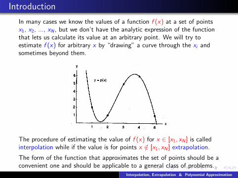
In many cases we know the values of a function f (x) at a set of pointsx1, x2, ..., xN , but we don’t have the analytic expression of the functionthat lets us calculate its value at an arbitrary point. We will try toestimate f (x) for arbitrary x by “drawing” a curve through the xi andsometimes beyond them.

The procedure of estimating the value of f (x) for x ∈ [x1, xN ] is calledinterpolation while if the value is for points x /∈ [x1, xN ] extrapolation.

The form of the function that approximates the set of points should be aconvenient one and should be applicable to a general class of problems.


Polynomial Approximations

Polynomial functions are the most common ones while rational andtrigonometric functions are used quite frequently.

We will study the following methods for polynomial approximations:

Lagrange’s Polynomial

Hermite Polynomial

Taylor Polynomial

Cubic Splines


Lagrange Polynomial

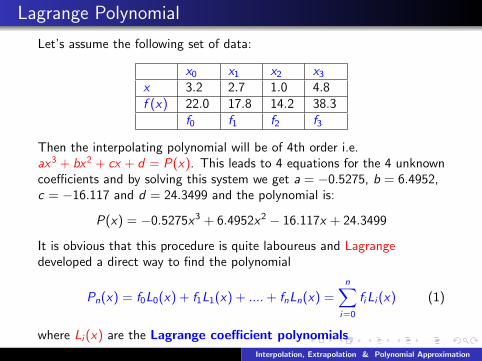
Let’s assume the following set of data:

x0 x1 x2 x3

x 3.2 2.7 1.0 4.8f (x) 22.0 17.8 14.2 38.3

f0 f1 f2 f3

Then the interpolating polynomial will be of 4th order i.e.ax3 + bx2 + cx + d = P(x). This leads to 4 equations for the 4 unknowncoefficients and by solving this system we get a = −0.5275, b = 6.4952,c = −16.117 and d = 24.3499 and the polynomial is:

P(x) = −0.5275x3 + 6.4952x2 − 16.117x + 24.3499

It is obvious that this procedure is quite laboureus and Lagrangedeveloped a direct way to find the polynomial

Pn(x) = f0L0(x) + f1L1(x) + ....+ fnLn(x) =n∑

i=0

fiLi (x) (1)

where Li (x) are the Lagrange coefficient polynomials


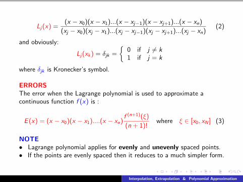
Lj(x) =(x − x0)(x − x1)...(x − xj−1)(x − xj+1)...(x − xn)

(xj − x0)(xj − x1)...(xj − xj−1)(xj − xj+1)...(xj − xn)(2)

and obviously:

Lj(xk) = δjk =

{0 if j 6= k1 if j = k

where δjk is Kronecker’s symbol.

ERRORSThe error when the Lagrange polynomial is used to approximate acontinuous function f (x) is :

E (x) = (x − x0)(x − x1)....(x − xn)f (n+1)(ξ)

(n + 1)!where ξ ∈ [x0, xN ] (3)

NOTE• Lagrange polynomial applies for evenly and unevenly spaced points.• If the points are evenly spaced then it reduces to a much simpler form.


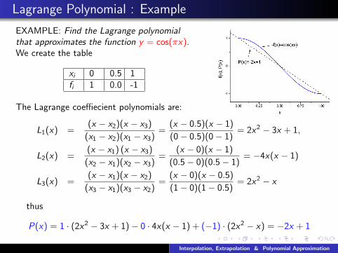
Lagrange Polynomial : Example

EXAMPLE: Find the Lagrange polynomialthat approximates the function y = cos(πx).We create the table

xi 0 0.5 1fi 1 0.0 -1

The Lagrange coeffiecient polynomials are:

L1(x) =(x − x2)(x − x3)

(x1 − x2)(x1 − x3)=

(x − 0.5)(x − 1)

(0− 0.5)(0− 1)= 2x2 − 3x + 1,

L2(x) =(x − x1) (x − x3)

(x2 − x1)(x2 − x3)=

(x − 0)(x − 1)

(0.5− 0)(0.5− 1)= −4x(x − 1)

L3(x) =(x − x1)(x − x2)

(x3 − x1)(x3 − x2)=

(x − 0)(x − 0.5)

(1− 0)(1− 0.5)= 2x2 − x

thus

P(x) = 1 · (2x2 − 3x + 1)− 0 · 4x(x − 1) + (−1) · (2x2 − x) = −2x + 1


The error will be:

E (x) = x · (x − 0.5) · (x − 1)π3 sin(πξ)

3!

e.g. for x = 0.25 is E (0.25) ≤ 0.24.


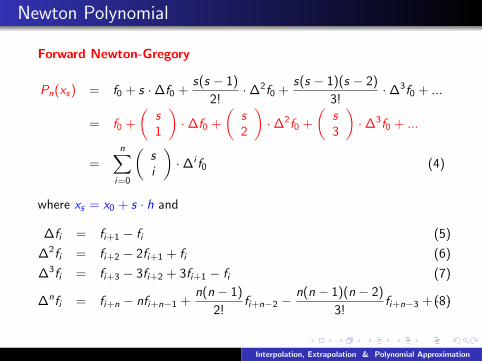
Newton Polynomial

Forward Newton-Gregory

Pn(xs) = f0 + s ·∆f0 +s(s − 1)

2!·∆2f0 +

s(s − 1)(s − 2)

3!·∆3f0 + ...

= f0 +

(s1

)·∆f0 +

(s2

)·∆2f0 +

(s3

)·∆3f0 + ...

=n∑

i=0

(si

)·∆i f0 (4)

where xs = x0 + s · h and

∆fi = fi+1 − fi (5)

∆2fi = fi+2 − 2fi+1 + fi (6)

∆3fi = fi+3 − 3fi+2 + 3fi+1 − fi (7)

∆nfi = fi+n − nfi+n−1 +n(n − 1)

2!fi+n−2 −

n(n − 1)(n − 2)

3!fi+n−3 + · · ·(8)


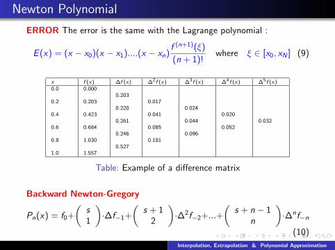
Newton Polynomial

ERROR The error is the same with the Lagrange polynomial :

E (x) = (x − x0)(x − x1)....(x − xn)f (n+1)(ξ)

(n + 1)!where ξ ∈ [x0, xN ] (9)

x f (x) ∆f (x) ∆2f (x) ∆3f (x) ∆4f (x) ∆5f (x)0.0 0.000

0.2030.2 0.203 0.017

0.220 0.0240.4 0.423 0.041 0.020

0.261 0.044 0.0320.6 0.684 0.085 0.052

0.246 0.0960.8 1.030 0.181

0.5271.0 1.557

Table: Example of a difference matrix

Backward Newton-Gregory

Pn(x) = f0+

(s1

)·∆f−1+

(s + 1

2

)·∆2f−2+...+

(s + n − 1

n

)·∆nf−n

(10)


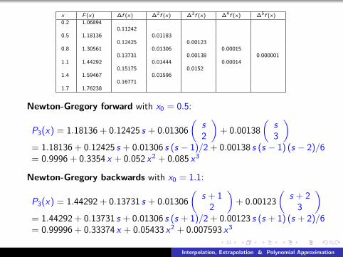
x F (x) ∆f (x) ∆2f (x) ∆3f (x) ∆4f (x) ∆5f (x)0.2 1.06894

0.112420.5 1.18136 0.01183

0.12425 0.001230.8 1.30561 0.01306 0.00015

0.13731 0.00138 0.0000011.1 1.44292 0.01444 0.00014

0.15175 0.01521.4 1.59467 0.01596

0.167711.7 1.76238

Newton-Gregory forward with x0 = 0.5:

P3(x) = 1.18136 + 0.12425 s + 0.01306

(s2

)+ 0.00138

(s3

)= 1.18136 + 0.12425 s + 0.01306 s (s − 1)/2 + 0.00138 s (s − 1) (s − 2)/6= 0.9996 + 0.3354 x + 0.052 x2 + 0.085 x3

Newton-Gregory backwards with x0 = 1.1:

P3(x) = 1.44292 + 0.13731 s + 0.01306

(s + 1

2

)+ 0.00123

(s + 2

3

)= 1.44292 + 0.13731 s + 0.01306 s (s + 1)/2 + 0.00123 s (s + 1) (s + 2)/6= 0.99996 + 0.33374 x + 0.05433 x2 + 0.007593 x3


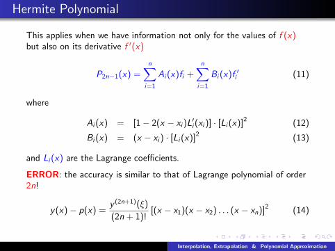
Hermite Polynomial

This applies when we have information not only for the values of f (x)but also on its derivative f ′(x)

P2n−1(x) =n∑

i=1

Ai (x)fi +n∑

i=1

Bi (x)f ′i (11)

where

Ai (x) = [1− 2(x − xi )L′i (xi )] · [Li (x)]2 (12)

Bi (x) = (x − xi ) · [Li (x)]2 (13)

and Li (x) are the Lagrange coefficients.

ERROR: the accuracy is similar to that of Lagrange polynomial of order2n!

y(x)− p(x) =y (2n+1)(ξ)

(2n + 1)![(x − x1)(x − x2) . . . (x − xn)]2 (14)


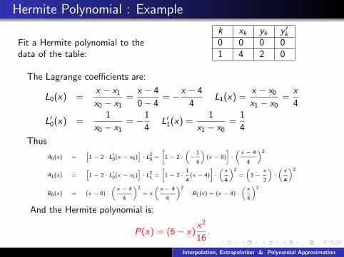
Hermite Polynomial : Example

Fit a Hermite polynomial to thedata of the table:

k xk yk y ′k0 0 0 01 4 2 0

The Lagrange coefficients are:

L0(x) =x − x1

x0 − x1=

x − 4

0− 4= −x − 4

4L1(x) =

x − x0

x1 − x0=

x

4

L′0(x) =1

x0 − x1= −1

4L′1(x) =

1

x1 − x0=

1

4

Thus

A0(x) =[

1 − 2 · L′0(x − x0)]· L2

0 =

[1 − 2 ·

(−

1

4

)(x − 0)

]·(

x − 4

4

)2

A1(x) =[

1 − 2 · L′0(x − x1)]· L2

1 =

[1 − 2 ·

1

4(x − 4)

]·(

x

4

)2=

(3 −

x

2

)·(

x

4

)2

B0(x) = (x − 0) ·(

x − 4

4

)2

= x

(x − 4

4

)2

B1(x) = (x − 4) ·(

x

4

)2

And the Hermite polynomial is:

P(x) = (6− x)x2

16.


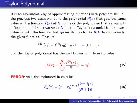
Taylor Polynomial

It is an alternative way of approximating functions with polynomials. Inthe previous two cases we found the polynomial P(x) that gets the samevalue with a function f (x) at N points or the polynomial that agrees witha function and its derivative at N points. Taylor polynomial has the samevalue x0 with the function but agrees also up to the Nth derivative withthe given function. That is:

P(i)(x0) = f (i)(x0) and i = 0, 1, ..., n

and the Taylor polynomial has the well known form from Calculus

P(x) =N∑i=0

f (i)(x)

i !(x − x0)i (15)

ERROR: was also estimated in calculus

EN(x) = (x − x0)N+1 f(N+1)(ξ)

(N + 1)!(16)


Taylor Polynomial : Example

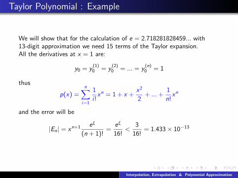
We will show that for the calculation of e = 2.718281828459... with13-digit approximation we need 15 terms of the Taylor expansion.All the derivatives at x = 1 are:

y0 = y(1)0 = y

(2)0 = ... = y

(n)0 = 1

thus

p(x) =n∑

i=1

1

i !xn = 1 + x +

x2

2+ ...+

1

n!xn

and the error will be

|En| = xn+1 eξ

(n + 1)!=

eξ

16!<

3

16!= 1.433× 10−13


Interpolation with Cubic Splines

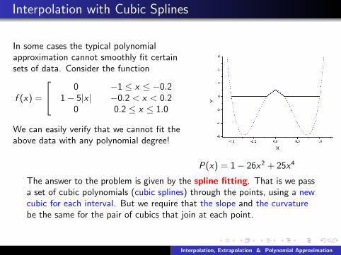
In some cases the typical polynomialapproximation cannot smoothly fit certainsets of data. Consider the function

f (x) =

0 −1 ≤ x ≤ −0.21− 5|x | −0.2 < x < 0.2

0 0.2 ≤ x ≤ 1.0

We can easily verify that we cannot fit theabove data with any polynomial degree!

P(x) = 1− 26x2 + 25x4

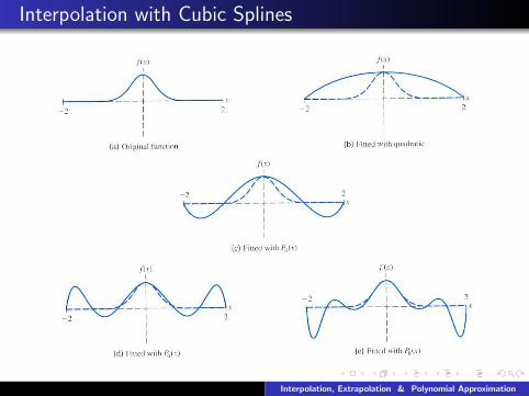
The answer to the problem is given by the spline fitting. That is we passa set of cubic polynomials (cubic splines) through the points, using a newcubic for each interval. But we require that the slope and the curvaturebe the same for the pair of cubics that join at each point.



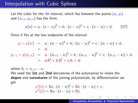
Let the cubic for the ith interval, which lies between the points (xi , yi )and (xi+1, yi+1) has the form:

y(x) = ai · (x − xi )3 + bi · (x − xi )

2 + ci · (x − xi ) + di (17)

Since it fits at the two endpoints of the interval:

yi = y(xi ) = ai · (xi − xi )3 + bi · (xi − xi )

2 + ci · (xi − xi ) + di

= di

yi+1 = y(xi+1) = ai · (xi+1 − xi )3 + bi · (xi+1 − xi )

2 + ci · (xi+1 − xi ) + di

= aih3i + bih

2i + cihi + di

where hi = xi+1 − xi .We need the 1st and 2nd derivatives of the polynomial to relate theslopes and curvatures of the joining polynomials, by differentiation weget

y ′(x) = 3ai · (x − xi )2 + 2bi · (x − xi ) + ci

y ′′(x) = 6ai · (x − xi ) + 2bi


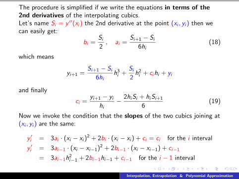
The procedure is simplified if we write the equations in terms of the2nd derivatives of the interpolating cubics.Let’s name Si = y ′′(xi ) the 2nd derivative at the point (xi , yi ) then wecan easily get:

bi =Si2, ai =

Si+1 − Si6hi

(18)

which means

yi+1 =Si+1 − Si

6hih3i +

Si2h2i + cihi + yi

and finally

ci =yi+1 − yi

hi− 2hiSi + hiSi+1

6(19)

Now we invoke the condition that the slopes of the two cubics joining at(xi , yi ) are the same:

y ′i = 3ai · (xi − xi )2 + 2bi · (xi − xi ) + ci = ci for the i interval

y ′i = 3ai−1 · (xi − xi−1)2 + 2bi−1 · (xi − xi−1) + ci−1

= 3ai−1h2i−1 + 2bi−1hi−1 + ci−1 for the i − 1 interval


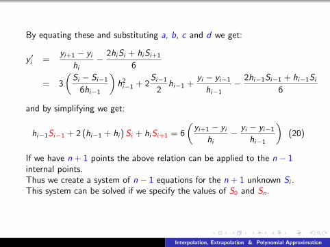
By equating these and substituting a, b, c and d we get:

y ′i =yi+1 − yi


6

= 3

(Si − Si−1

6hi−1

)h2i−1 + 2

Si−1

2hi−1 +

yi − yi−1

hi−1− 2hi−1Si−1 + hi−1Si

6

and by simplifying we get:

hi−1Si−1 + 2 (hi−1 + hi )Si + hiSi+1 = 6

(yi+1 − yi

hi− yi − yi−1

hi−1

)(20)

If we have n + 1 points the above relation can be applied to the n − 1internal points.Thus we create a system of n − 1 equations for the n + 1 unknown Si .This system can be solved if we specify the values of S0 and Sn.


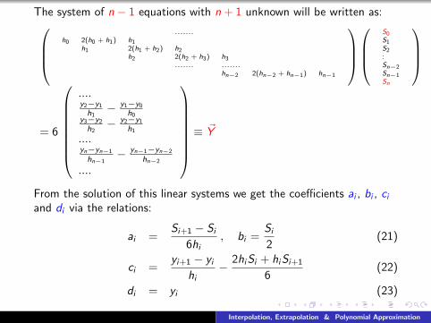
The system of n − 1 equations with n + 1 unknown will be written as:.......

h0 2(h0 + h1) h1h1 2(h1 + h2) h2

h2 2(h2 + h3) h3....... .......

hn−2 2(hn−2 + hn−1) hn−1

S0S1S2:Sn−2Sn−1Sn

= 6

....y2−y1

h1− y1−y0

h0y3−y2

h2− y2−y1

h1

....yn−yn−1

hn−1− yn−1−yn−2

hn−2

....

≡ ~Y

From the solution of this linear systems we get the coefficients ai , bi , ciand di via the relations:

ai =Si+1 − Si

6hi, bi =

Si2

(21)

ci =yi+1 − yi


6(22)

di = yi (23)


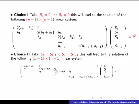
• Choice I Take, S0 = 0 and Sn = 0 this will lead to the solution of thefollowing (n − 1)× (n − 1) linear system:

2(h0 + h1) h1

h1 2(h1 + h2) h2

h2 2(h2 + h3) h3

....hn−2 2(hn−2 + hn−1)

·

S1

S2

S3

Sn−1

= ~Y

• Choice II Take, S0 = S1 and Sn = Sn−1 this will lead to the solution ofthe following (n − 1)× (n − 1) linear system:

3h0 + 2h1 h1h1 2(h1 + h2) h2

h2 2(h2 + h3) h3... ...

hn−2 2hn−2 + 3hn−1

S1S2S3

Sn−1

= ~Y


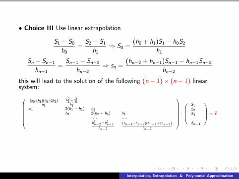
• Choice III Use linear extrapolation

S1 − S0

h0=

S2 − S1

h1⇒ S0 =

(h0 + h1)S1 − h0S2

h1

Sn − Sn−1

hn−1=

Sn−1 − Sn−2

hn−2⇒ sn =

(hn−2 + hn−1)Sn−1 − hn−1Sn−2

hn−2

this will lead to the solution of the following (n − 1)× (n − 1) linearsystem:

(h0+h1)(h0+2h1)h1

h21−h2

0h1

h1 2(h1 + h2) h2h2 2(h2 + h3) h3

.... ....h2n−2−h2

n−1hn−2

(hn−1+hn−2)(hn−1+2hn−2)

hn−2

·

S1S2S3

Sn−1

= ~Y


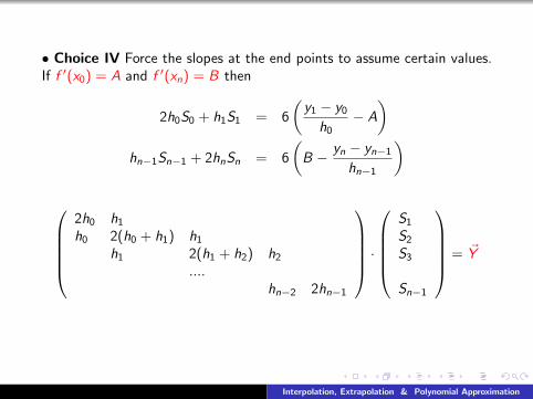
• Choice IV Force the slopes at the end points to assume certain values.If f ′(x0) = A and f ′(xn) = B then

2h0S0 + h1S1 = 6

(y1 − y0

h0− A

)hn−1Sn−1 + 2hnSn = 6

(B − yn − yn−1

hn−1

)

2h0 h1

h0 2(h0 + h1) h1

h1 2(h1 + h2) h2

....hn−2 2hn−1

·

S1

S2

S3

Sn−1

= ~Y


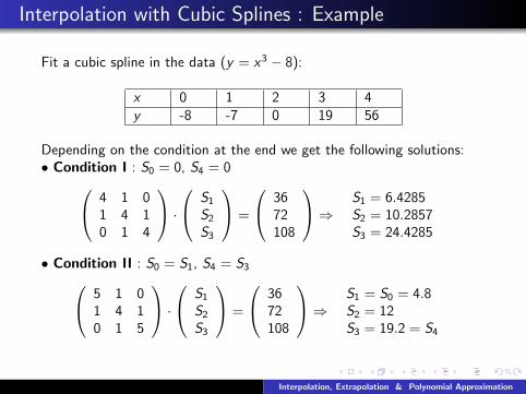
Interpolation with Cubic Splines : Example

Fit a cubic spline in the data (y = x3 − 8):

x 0 1 2 3 4y -8 -7 0 19 56

Depending on the condition at the end we get the following solutions:• Condition I : S0 = 0, S4 = 0 4 1 0

1 4 10 1 4

· S1

S2

S3

=

3672108

⇒ S1 = 6.4285S2 = 10.2857S3 = 24.4285

• Condition II : S0 = S1, S4 = S3 5 1 01 4 10 1 5

· S1

S2

S3

=

3672108

⇒ S1 = S0 = 4.8S2 = 12S3 = 19.2 = S4


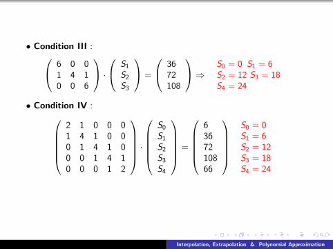
• Condition III : 6 0 01 4 10 0 6

· S1

S2

S3

=

3672108

⇒ S0 = 0 S1 = 6S2 = 12 S3 = 18S4 = 24

• Condition IV :2 1 0 0 01 4 1 0 00 1 4 1 00 0 1 4 10 0 0 1 2

·

S0

S1

S2

S3

S4

=

6367210866

S0 = 0S1 = 6S2 = 12S3 = 18S4 = 24


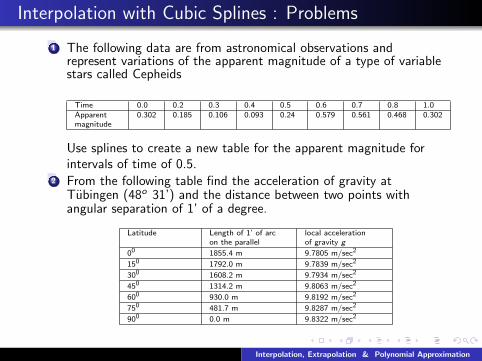
Interpolation with Cubic Splines : Problems

1 The following data are from astronomical observations andrepresent variations of the apparent magnitude of a type of variablestars called Cepheids

Time 0.0 0.2 0.3 0.4 0.5 0.6 0.7 0.8 1.0Apparentmagnitude

0.302 0.185 0.106 0.093 0.24 0.579 0.561 0.468 0.302

Use splines to create a new table for the apparent magnitude forintervals of time of 0.5.

2 From the following table find the acceleration of gravity atTubingen (48o 31’) and the distance between two points withangular separation of 1’ of a degree.

Latitude Length of 1’ of arcon the parallel

local accelerationof gravity g

00 1855.4 m 9.7805 m/sec2

150 1792.0 m 9.7839 m/sec2

300 1608.2 m 9.7934 m/sec2

450 1314.2 m 9.8063 m/sec2

600 930.0 m 9.8192 m/sec2

750 481.7 m 9.8287 m/sec2

900 0.0 m 9.8322 m/sec2


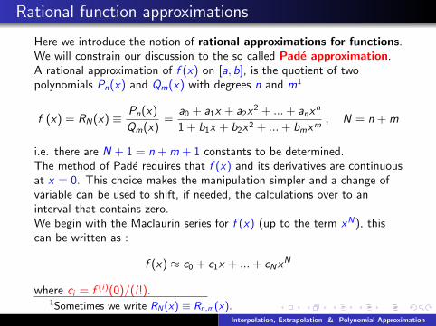
Rational function approximations

Here we introduce the notion of rational approximations for functions.We will constrain our discussion to the so called Pade approximation.A rational approximation of f (x) on [a, b], is the quotient of twopolynomials Pn(x) and Qm(x) with degrees n and m1

f (x) = RN(x) ≡ Pn(x)

Qm(x)=

a0 + a1x + a2x2 + ...+ anx

n

1 + b1x + b2x2 + ...+ bmxm, N = n + m

i.e. there are N + 1 = n + m + 1 constants to be determined.The method of Pade requires that f (x) and its derivatives are continuousat x = 0. This choice makes the manipulation simpler and a change ofvariable can be used to shift, if needed, the calculations over to aninterval that contains zero.We begin with the Maclaurin series for f (x) (up to the term xN), thiscan be written as :

f (x) ≈ c0 + c1x + ...+ cNxN

where ci = f (i)(0)/(i !).1Sometimes we write RN(x) ≡ Rn,m(x).


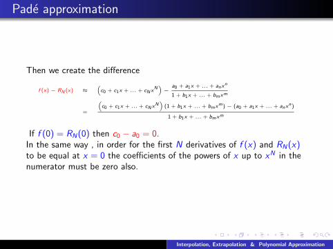
Pade approximation

Then we create the difference

f (x) − RN (x) ≈(c0 + c1x + ... + cN xN

)−

a0 + a1x + ... + anxn

1 + b1x + ... + bmxm

=

(c0 + c1x + ... + cN xN

)(1 + b1x + ... + bmxm) − (a0 + a1x + ... + anx

n)

1 + b1x + ... + bmxm

If f (0) = RN(0) then c0 − a0 = 0.In the same way , in order for the first N derivatives of f (x) and RN(x)to be equal at x = 0 the coefficients of the powers of x up to xN in thenumerator must be zero also.


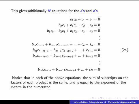
This gives additionally N equations for the a’s and b’s

b1c0 + c1 − a1 = 0

b2c0 + b1c1 + c2 − a2 = 0

b3c0 + b2c1 + b1c2 + c3 − a3 = 0...

bmcn−m + bm−1cn−m+1 + ...+ cn − an = 0

bmcn−m+1 + bm−1cn−m+2 + ...+ cn+1 = 0 (24)

bmcn−m+2 + bm−1cn−m+3 + ...+ cn+2 = 0

...

bmcN−m + bm−1cN−m+1 + ...+ cN = 0

Notice that in each of the above equations, the sum of subscripts on thefactors of each product is the same, and is equal to the exponent of thex-term in the numerator.


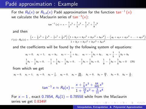
Pade approximation : Example

For the R9(x) or R5,4(x) Pade approximation for the function tan−1 (x)we calculate the Maclaurin series of tan−1(x):

tan−1 (x) = x −1

3x3 +

1

5x5 −

1

7x7 +

1

9x9

and then

f (x)−R9 (x) =

(x − 1

3x3 + 1

5x5 − 1

7x7 + 1

9x9) (

1 + b1x + b2x2 + b3x

3 + b4x4)−(a0 + a1x + a2x

2 + ... + a5x5)

1 + b1x + b2x2 + b3x3 + b4x4

and the coefficients will be found by the following system of equations:

a0 = 0, a1 = 1, a2 = b1, a3 = −1

3+ b2 , a4 = −

1

3b1 + b3 , a5 =

1

5−

1

3b2 + b4

1

5b1 −

1

2b3 = 0, −

1

7+

1

5b2 −

1

3b4 = 0 , −

1

7b1 +

1

5b3 = 0,

1

9−

1

7b2 +

1

5b4 = 0 (25)

from which we get

a0 = 0, a1 = 1, a2 = 0, a3 = 79, a4 = 0, a5 = 64

945, b1 = 0, b2 = 10

9, b3 = 0, b4 = 5

21.

tan−1 x ≈ R9(x) =x + 7

9x3 + 64

945x5

1 + 109 x2 + 5

21x4

For x = 1 , exact 0.7854, R9(1) = 0.78558 while from the Maclaurinseries we get 0.8349!


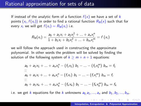
Rational approximation for sets of data

If instead of the analytic form of a function f (x) we have a set of kpoints (xi , f (xi )) in order to find a rational function RN(x) such that forevery xi we will get f (xi ) = RN(xi ) i.e.

RN(xi ) =a0 + a1xi + a2x

2i + ...+ anx

ni

1 + b1xi + b2x2i + ...+ bmxmi

= f (xi )

we will follow the approach used in constructing the approximatepolynomial. In other words the problem will be solved by finding thesolution of the following system of k ≥ m + n + 1 equations:

a0 + a1x1 + ...+ anxn1 − (f1x1) b1 − ...− (f1x

m1 ) bm = f1

::a0 + a1xi + ...+ anx

ni − (fixi ) b1 − ...− (fix

mi ) bm = fi

::a0 + a1xk + ...+ anx

nk − (fkxk) b1 − ...− (fkx

mk ) bm = fk

i.e. we get k equations for the k unknowns a0,a1, ..., an and b1, b2, ..., bm.


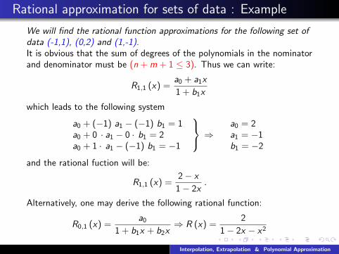
Rational approximation for sets of data : Example

We will find the rational function approximations for the following set ofdata (-1,1), (0,2) and (1,-1).It is obvious that the sum of degrees of the polynomials in the nominatorand denominator must be (n + m + 1 ≤ 3). Thus we can write:

R1,1 (x) =a0 + a1x

1 + b1x

which leads to the following system

a0 + (−1) a1 − (−1) b1 = 1a0 + 0 · a1 − 0 · b1 = 2a0 + 1 · a1 − (−1) b1 = −1

⇒ a0 = 2a1 = −1b1 = −2

and the rational fuction will be:

R1,1 (x) =2− x

1− 2x.

Alternatively, one may derive the following rational function:

R0,1 (x) =a0

1 + b1x + b2x⇒ R (x) =

2

1− 2x − x2


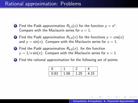
Rational approximation: Problems

1 Find the Pade approximation R3,3(x) for the function y = ex .Compare with the Maclaurin series for x = 1.

2 Find the Pade approximation R3,5(x) for the functions y = cos(x)and y = sin(x). Compare with the Maclaurin series for x = 1.

3 Find the Pade approximation R4,6(x). for the functiony = 1/x sin(x). Compare with the Maclaurin series for x = 1.

4 Find the rational approximation for the following set of points:

0 1 2 40.83 1.06 1.25 4.15


interpolation, extrapolation & polynomial approximation

Documents