interpolation in riemannian manifoldsshreya bhattarai (candidate) w prof. lyle noakes (supervisor) 3...

Interpolation in RiemannianManifolds

Shreya Bhattarai

This thesis is presented for the degree ofDoctor of Philosophy

of The University of Western AustraliaDepartment of Mathematics and Statistics

2013

2

Candidate’s statement of contribution

Chapter 3 in this thesis is a paper submitted for publication, which I jointlyauthored as primary author, with my supervisor W. Prof Lyle Noakes.All other chapters in the thesis are the result of my own work but with a lot ofhelp from weekly discussions with Prof. Noakes.

Shreya Bhattarai (candidate)

W Prof. Lyle Noakes (supervisor)

3

Abstract

It is a very natural task to connect the dots between patterns of data we see.This fundamental procedure of connecting the dots, or interpolation, arises inmany contexts including graphics, robot path planning, and medical imagining.Although the subject of interpolation has been thoroughly studied for Euclideanspaces, the more general setting of interpolating in a Riemannian manifold hasonly relatively recently received attention. The central aim of this thesis is topresent results concerning the interpolation of data points in Riemannian mani-folds, and in particular Lie groups.

Riemannian manifolds are smooth spaces where concepts such as distancesand angles are defined using a metric. A dynamical system’s state can often berepresented as points in a Riemannian manifold and we can apply geometricalmethods of inference to predict how the system would have behaved given a suit-able model of the dynamics. This thesis in a broad sense looks at various ways tomodel a system’s dynamical behaviour in order to interpolate effectively.

Chapter 3 concerns null Riemannian cubics in tension. Null Riemannian cu-bics in tension are a special sub-class of Riemannian cubics in tension and arethe differential analogues of hyperbolic trigonometric functions, which are usedto produce differentiable interpolants. Asymptotic behaviour of the curves arederived.

Chapter 4 concerns ways to incorporate dynamical systems into the interpola-tion scheme using the notion of a prior vector field. If a differential equation whichattempts to model a dynamical system is specified by a vector field, then a nat-ural choice of interpolant is one which minimises the error in the equation beingsatisfied. Several different frameworks, including second order and time varyingsystems, are considered and some necessary conditions concerning the solutionsare described in the case of Lie groups.

Chapter 5 builds on the results of Chapters 3 and 4 by implementing aninterpolation scheme based on a linearisation of the differential equation. Weapproximate natural conditional extremal splines and natural Riemannian cubicsin tension splines using an analogue of the traditional B-spline methodology andanalyse how effective the method is.

Chapter 6 focuses on discretisation of spaces of curves and outlines relation-ships between the continuous and discretised problem. An alternative methodto produce interpolants using numerical optimization packages on (large) finitedimensional spaces is considered which allows for a much broader scope for appli-cations. The results produced are compared to those of the previous chapter.

4

Acknowledgements

There are so many people who made it possible for me to finish my PhD. Thereis no possible way to thank everyone in the amount of words that I feel they eachdeserve.

First and foremost I would like to thank my supervisor, W Prof. Lyle Noakeswho has shown me unimaginable amounts of care and patience. With your guid-ance and love for mathematics, you have made completing my PhD an extremelyenjoyable experience and have taught me how to always bring out the best inother people.

I would also like to thank my examiners Prof. Anthony Bloch, Prof. MarinKobilarov, and Dr. Cesare Tronci. Your valuable suggestions and feedback haveproven invaluable and provide a wealth of future directions for study.

I would like to acknowledge and thank the University of Western Australiaand the Australian government for allowing me to study under a University Post-graduate Scholarship and Australian Postgraduate Scholarship.

To Dad, Mum, and my brother Debesh, thanks for the unceasing encourage-ment and support.

I would also like to thank the many friends whom I have had the pleasure ofsharing this time with. To the ‘amigos’ Brian Corr, Yohei Negi, Philip Schrader,Michael Pauley, and Ryan Mickler. Without each of you, life at university wouldbe a major drag. To my past and present housemates Trent, Vlad, Chris, Steveand Matt. Thanks for the company and all the conversations. To Kenny, Tony,Sean, John, Adam, Bucky, Smriti, Jess, Anthony, Rohan(s), Sham, and all theothers who I have missed, you made the last few years the best years of my life. ToHua, for being an excellent Go teacher and friend. To the ‘crossword gang’, Rob,Con and all the friendly staff at UWA who made lunch times quite memorable.

Lastly I would like to thank my beautiful girlfriend Rijbi Dixit who was alwaysthere to help me and clear any doubts I may ever had had.

5

Contents

0.1 Notation . . . . . . . . . . . . . . . . . . . . . . . . . . . . . . . . 7

1 Riemannian Geometry and Lie Groups . . . . . . . . . . . . . . . 9

1.1 Smooth Manifolds . . . . . . . . . . . . . . . . . . . . . . . . . . . 9

1.2 Riemannian Geometry . . . . . . . . . . . . . . . . . . . . . . . . 13

1.3 Calculus of Variations . . . . . . . . . . . . . . . . . . . . . . . . 14

1.3.1 First order Lagrangians and the Euler-Lagrange Equations 14

1.3.2 Hamiltonian Formalism . . . . . . . . . . . . . . . . . . . . 15

1.4 Lie algebras and Lie groups . . . . . . . . . . . . . . . . . . . . . 16

1.4.1 Matrix Lie groups . . . . . . . . . . . . . . . . . . . . . . . 20

1.4.2 Lax constraints . . . . . . . . . . . . . . . . . . . . . . . . 20

2 Literature Review . . . . . . . . . . . . . . . . . . . . . . . . . . . . 23

2.1 Interpolation in Manifolds . . . . . . . . . . . . . . . . . . . . . . 23

2.2 Riemannian Cubics in Tension . . . . . . . . . . . . . . . . . . . . 26

2.3 Prior fields . . . . . . . . . . . . . . . . . . . . . . . . . . . . . . . 27

3 Asymptotics of Null Riemannian Cubics in Tension in SO(3) . 29

3.1 Introduction . . . . . . . . . . . . . . . . . . . . . . . . . . . . . . 29

3.1.1 Null Riemannian Cubics in Tension and their connection to

other families of curves . . . . . . . . . . . . . . . . . . . . 33

3.2 Asymptotics of Null Lie Quadratics in Tension in so(3) . . . . . . 37

3.3 Asymptotics of Null Riemannian Cubics in Tension in SO(3) . . . 43

3.4 Conclusion . . . . . . . . . . . . . . . . . . . . . . . . . . . . . . . 47

4 Prior fields . . . . . . . . . . . . . . . . . . . . . . . . . . . . . . . . . 49

4.1 Introduction . . . . . . . . . . . . . . . . . . . . . . . . . . . . . . 49

4.2 First order systems . . . . . . . . . . . . . . . . . . . . . . . . . . 49

4.2.1 Variable left-invariant priors . . . . . . . . . . . . . . . . . 63

4.3 Second order systems . . . . . . . . . . . . . . . . . . . . . . . . . 64

6 CONTENTS

4.4 Time varying systems . . . . . . . . . . . . . . . . . . . . . . . . . 66

4.4.1 Time varying prior fields for solvable A(t) in a bi-invariant

Lie group . . . . . . . . . . . . . . . . . . . . . . . . . . . 71

4.4.2 Time varying prior fields in SO(3) . . . . . . . . . . . . . . 73

4.4.3 Second order time-variant systems . . . . . . . . . . . . . 77

4.5 Conclusion . . . . . . . . . . . . . . . . . . . . . . . . . . . . . . . 79

5 Linear interpolation schemes on bi-invariant Lie groups . . . . 81

5.1 Introduction . . . . . . . . . . . . . . . . . . . . . . . . . . . . . 81

5.2 Second order prior fields in SO(3) . . . . . . . . . . . . . . . . . . 82

5.2.1 A(t) = constant. . . . . . . . . . . . . . . . . . . . . . . . 84

5.3 Approximating natural Riemannian cubics in tension splines . . . 97

5.4 Conclusion . . . . . . . . . . . . . . . . . . . . . . . . . . . . . . . 100

6 Numerical Interpolation Schemes for Second Order Lagrangians101

6.1 Introduction . . . . . . . . . . . . . . . . . . . . . . . . . . . . . 101

6.2 Approximations of derivatives . . . . . . . . . . . . . . . . . . . . 102

6.3 Unconstrained optimisation . . . . . . . . . . . . . . . . . . . . . 104

6.4 Constrained optimisation . . . . . . . . . . . . . . . . . . . . . . . 107

6.4.1 Case study: AJ2 on S3 . . . . . . . . . . . . . . . . . . . . 107

6.5 Conclusion . . . . . . . . . . . . . . . . . . . . . . . . . . . . . . . 110

7 Conclusions . . . . . . . . . . . . . . . . . . . . . . . . . . . . . . . . 113

Bibliography . . . . . . . . . . . . . . . . . . . . . . . . . . . . . . . . . 117

0.1. Notation 7

0.1 Notation

Quick reference table for frequently used notation

Q Manifold

U Neighbourhoods of Q

q Points in Q

v Vectors in TQ

X ,Y ,Z Smooth vector fields on Q

n Dimension of Q

f (k) The kth derivative of f

α, β Set index variables

G Lie groups

g, h Lie group elements (or sometimes functions)

g Lie algebras

A,B,C,D Lie algebra variables

[A,B] Lie bracket of A and B

Adg : g→ g Adjoint action of g: AdgA = dLg dRg−1A

adA : g→ g Adjoint action of A: adAB = [A,B]

〈v0, v1〉 Inner product of v0 and v1

I The unit interval

Ik×k The k × k identity matrix

e Lie group identity element

Ckq0,q1

Space of Ck curves connecting q0 and q1

x(t) A curve x in the manifold parameterised by t

γ(t) Geodesics in Q

X(t),W (t) Vector field along x(t)

V (t) The left Lie reduction of x(1)(t)

N Number of intervals to be interpolated

ξ = (ξ0, . . . , ξN) Data set of points to be interpolated

Jk The kth order energy functional

Jλ2 Riemannian cubic in tension functional with tension λ

AJk The kth order prior field functional

8 CONTENTS

9CHAPTER 1

Riemannian Geometry and Lie Groups

1.1 Smooth Manifolds

Manifolds are spaces which locally look like Euclidean space but globally may

have different structure. Typically manifolds arise in physical systems satisfying

nonlinear constraints such as conservation laws, and come equipped with addi-

tional structure, such as Riemannian metrics or symplectic forms. We will be

interested in studying interpolation in manifolds and so we will only consider con-

nected spaces.

Formally, an n-dimensional smooth manifold is a topological space Q with an open

cover Uα and a collection of homeomorphisms φα : Uα → Rn such that each of

the maps φαφ−1β : Rn → Rn are smooth. The pairs (Uα, φα) are called charts. We

say the standard Euclidean coordinates (u1, . . . , un) are a local coordinate system

on Uα where (u1, . . . , un) represents φ(u1, . . . , un). A map between manifolds is

considered smooth if the induced maps between all choices of coordinate charts

are also smooth in the standard sense of maps between open subsets of Rn and

Rm.

Let x1, x2 : (−1, 1) → Q be two curves such that x1(0) = x2(0) = q. We say

they are equivalent at q if we have (φα x1)′(0) = (φα x2)′(0). It can be

shown that this definition does not depend on the chart. Equivalence classes

of these curves are called tangent vectors at q and the set of tangent vectors

at q can be made into a vector space by setting [x1(t)] + [x2(t)] = [x3(t)] when

we have (φα x1)′(0) + (φα x2)′(0) = (φα x3)′(0) and r[x1(t)] = [x2(t)] when

r(φα x1)′(0) = (φα x2)′(0) for all r ∈ R. We denote the set of tangent vectors

at q by TqQ. Let q = (u1, ..., un) in a choice of local coordinates, then a basis

for TqQ will be ∂i := [(u1, . . . , ui + t, . . . , un)] for i = 1, . . . , n. Let v ∈ TqQ and

f : Q→ R, then define vf := (f v)′(0) where v is any representative curve of v.

The operation of v is independent of choice of v, and so tangent vectors can be

thought of as differential operators, and ∂i as partial derivatives in a coordinate

system. Any tangent vector v can be written with respect to local coordinates as

10 Chapter 1. Riemannian Geometry and Lie Groups

vi∂i.

We can define the tangent bundle TQ of Q to be the disjoint union of tangent

spaces TqQ, that is, TQ = ∪q∈Qq × TqQ. There is a natural projection map

π : TQ → Q given by π(q, v) = q. The tangent bundle has a natural topology

and can be made into a manifold itself.

A vector field X on Q is a smooth section of the tangent bundle. That is to say,

X : Q→ TQ is a smooth map and πQ = id. A derivation D : C∞(Q)→ C∞(Q)

is a map such that D(f + g) = Df + Dg and D(fg) = fDg + gDf . The

space of smooth vector fields form a vector space denoted X(Q) and they are in

one to one correspondence with the space of derivations with the identification

(X f)(q) = X (q)f (See [36, Addendum] for a proof). The flow Φ of a vector field

X is a map Φt : Q → Q defined by the differential equation ddt

Φt(q0) = XΦt(q0)

with Φ0(q0) = q0. The question of when Φt is defined is answered in [36] which

says that if Q is a Hausdorff manifold, there is a continuous function ε : Q→ R+

such that Φt(q0) is defined when |t| < ε(q0). Moreover, Φs Φt = Φs+t when they

are defined. Specific trajectories generated by a flow are also called integral curves

of X .

Given two vector fields X ,Y , we can define their Lie bracket [X ,Y ] by the for-

mula [X ,Y ]f = X (Yf) − Y(X f) for all f ∈ C∞(Q). It can be shown that

[X ,Y ] is well defined and is in fact a vector field. With this operation, the space

X(Q) is a Lie algebra (See section 1.4). The advantage of thinking of vector

fields as derivations is that derivations have a natural Lie bracket operation.

The Lie bracket of two vector fields X and Y can be informally thought of as

a measure of the failure of flows of X and Y to commute. More formally, let

Φ and Ψ be the flows of X and Y respectively. Then we have for any chart,

(Ψ−t Φ−t Ψt Φt)x0 = x0 + t2[X ,Y ] +O(t3).

A more general notion than that of a tangent bundle is that of a vector bundle.

A quadruple E = (E,Q, π, F ) is called a smooth vector bundle when both the

total space E and the base space Q are smooth manifolds and π : E → Q is a

smooth surjection such that π−1(q), the fiber over q, has a vector space structure

1.1. Smooth Manifolds 11

which is isomorphic to the fiber space F . Moreover we require that for any point

in Q, there is a neighbourhood U of that point and map φ such that the following

diagram commutes:

π−1(U)φ- U × F

U

pr1

?

π-

where pr1 is the projection onto the first component. Moreover, for any point q

in U , the map v 7→ φ−1(q, v) is a linear isomorphism between F and π−1(q). Such

(U, φ) are called local trivializations. An example of a smooth vector bundle is

TQ = (TQ,Q, π,Rn). We define a smooth section of a bundle to be a smooth

map s : Q → E such that π s = id. The space of all smooth sections on E is

denoted by Γ(E), for example Γ(TQ) = X(Q).

Let π : E → Q be a vector bundle and let f : Q′ → Q be a continuous map.

Then the pullback bundle is defined by f ∗E = (q, v) ∈ Q′×E|f(q) = π(v) with

the topology on f ∗E being defined by the subspace topology and the projection

map π′ : f ∗E → Q′ given by projection onto the first factor. Given two vector

bundles E1, E2 over the same base space, we are able to construct the Whitney

sum E1 ⊕ E2 of the bundles and the tensor product E1 ⊗ E2. The Whitney sum

E1 ⊕ E2 has fiber over q equal to π−11 (q) ⊕ π−1

2 (q). Similarly the tensor product

E1 ⊗ E2 has fiber over q equal to π−11 (q) ⊗ π−1

2 (q). We can also take the dual

bundle, E∗, where fibers over q equal (π−1(q))∗. For more details regarding the

construction of these spaces, see [45].

For any vector bundle E and natural numbers r, s, define the tensor bundle of

type (r, s) as follows:

T srE = E∗ ⊗ · · · ⊗ E∗︸︷︷︸r

⊗E ⊗ · · · ⊗ E︸︷︷︸s

(1.1)


Sections of such a bundle are called tensor fields and we will refer to the space of

all tensor fields ΓsrE. Such a tensor field is said to have r contravariant indices

and s covariant indices.

A R-linear mapping ∇ : ΓE → Γ(TQ∗⊗E) is called a connection if it satisfies the

the Leibniz identity ∇fs = df ⊗ s + f∇s for all f ∈ C∞(Q) and s ∈ ΓE where

d is the exterior derivative. That is to say, given a section s, ∇s is an element of

Γ(TQ∗⊗E). This allows us to define the covariant derivative ∇X s for any vector

field X and section s by contracting ∇s with X , resulting in another section.

Given a connection on a manifold, we have a covariant derivative ∇ : X(Q) ×

X(Q)→ X(Q) which satisfies the following properties:

∇fX1+gX2Y = f∇X1Y + g∇X2Y ∀f, g ∈ C∞(Q) (1.2)

∇XfY = f∇XY + (X f)Y ∀f ∈ C∞(Q) (1.3)

∇X (aY1 + bY2) = a∇XY1 + b∇XY2 ∀a, b ∈ R (1.4)

Informally we can think of ∇XY as differentiating the vector field Y in the di-

rection of X . (∇XY)(q) depends only on X (q) and on Y in a neighbourhood

of q. In local coordinates, the connection defines n3 smooth functions Γkij where

∇∂i∂j = Γkij∂k. We say the connection is torsion-free (or symmetric) when

∇XY −∇YX = [X ,Y ] ∀X ,Y ∈ X(Q) (1.5)

Let x be a curve in Q. We can then define the notion of vector fields over x. We

say X is a smooth vector field over or along x when X(t) ∈ Tx(t)Q and the map

t 7→ X(t)f is smooth for any f ∈ C∞(Q). Then we can define a new vector field

along x called the covariant derivative of X along x by ∇x(1)X, denoted ∇tX for

short. In local coordinates let X(t) = X i(t)∂i. Then ∇tX(t) is defined by

∇tX(t) := (X i)(1)(t)∂i +X i∇x(1)(t)∂i. (1.6)

Covariant differentiation allows us to define the important notion of parallel trans-

1.2. Riemannian Geometry 13

porting a vector. If we have a vector field X(t) along x(t) such that ∇tX = 0,

then X(t) is said to have been obtained by parallel transporting X(t0) along x(t).

We can write ΠtxX(t0) = X(t).

1.2 Riemannian Geometry

Riemannian geometry is the study of manifolds for which we have a notion of

inner products between vectors tangent to some point. A Riemannian metric is a

smooth contravariant 2-tensor field g which is symmetric and positive definite on

each tangent space. Such a metric defines an inner product at each tangent space

TqQ given by 〈v, w〉 = gq(v, w) for v, w ∈ TqQ. A smooth manifold together with

a Riemannian metric (Q, g) is called a Riemannian manifold.

Given a Riemannian metric, we say a connection is compatible with the metric

when

X〈Y ,Z〉 = 〈∇XY ,Z〉+ 〈Y ,∇XZ〉 for all X ,Y ,Z ∈ X(Q). (1.7)

Theorem 1.2.1 (Fundamental Theorem of Riemannian Geometry [18]). A Rie-

mannian manifold has a unique torsion-free connection compatible with the metric

This torsion free and symmetric connection is known as the Levi-Civita con-

nection.

For the Levi-Civita connection, if X and Y are parallelly transported vector fields

along x(t), then compatibility of the metric implies that 〈X(t), Y (t)〉 is fixed along

x. Let x be a small loop with x(t0) = x(t1). Now consider parallel transporting

a vector v around this loop. Generally, v and the transported vector will differ.

The curvature tensor is a measure of this effect to first order accuracy. Define the

curvature R as a (3, 1) tensor field:

R(X ,Y)Z = ∇X∇YZ −∇Y∇XZ −∇[X ,Y]Z (1.8)

It is easily verified (See [18, Section 9]) that such a map depends on X ,Y ,Z only at

a point q and so it is indeed a tensor field. Choose a surface σ : [0, 1]× [0, 1]→ Q

parameterised by r and s and define X = ∂σdr

and Y = ∂σds

. Define a curve


xh : [0, 1]→ Q to be a traversing of the boundary of the image of [0, h]×[0, h] under

σ. Then the Ambrose-Singer theorem [46] says that d2

dh2Π1xv − v|r=0 = R(X, Y )v

where Π1xv is the parallel transport of v done piecewise along xh(t).

1.3 Calculus of Variations

1.3.1 First order Lagrangians and the Euler-Lagrange Equations

In Lagrange’s formulation of classical mechanics, we are to consider paths that

minimise the integral of a function L : TQ × R → R known as a (first order)

Lagrangian. Classically the Lagrangian is given as the kinetic energy minus

the potential energy. For example, for a particle moving in a potential field,

L(q, v, t) = 12m‖v‖2 − V (q). We are interested in finding curves x : [0, 1] → Q

that minimise the following functional

J(x) =

∫ 1

0

L(x(t), x(1)(t), t)dt (1.9)

over curves x(t) satisfying the boundary constraint x(0) = q0 and x(1) = q1.

Define a variation of a curve x as a smooth family of curves xh parameterised by

h ∈ (−ε, ε) where x0 = x. A necessary property of such a minimising curve x is

that for any variation xh, the derivative of J with respect to h must vanish at

h = 0. Moreover, any curve x that minimises J also minimises the functional that

is given by the same integrand but on a subinterval (t0, t1) ⊆ [0, 1]. Let X(t) be

a vector field along x(t) vanishing at t = t0, t1. Now define xh to be any family of

curves subject to the condition that ddh

∣∣h=0

xh(t) = X(t). Choose a local coordinate

system containing the curve segment between [t0, t1] where xh(t) = uh(t) and let

Lq and Lv be the corresponding partial derivatives of L.

dJ(xh)

dh=

d

dh

∫ t1

t0

L(uh, u(1)h , t)dt

=

∫ t1

t0

d

dhL(uh, u

(1)h , t)dt

=

∫ t1

t0

(Lq(uh, u

(1)h , t)

duhdh

+ Lv(uh, u(1)h , t)

du(1)h

dh

)dt

1.3. Calculus of Variations 15

=

∫ t1

t0

(Lq(uh, u

(1)h , t)− d

dtLv(uh, u

(1)h , t)

)duhdh

dt

The last step uses integration by parts and the fact that duhdh

vanishes at the

endpoints of the variation. Evaluating at h = 0, we see

dJ

dh|h=0

∫ t1

t0

(Lx(u, u

(1), t)− d

dtLv(u, u

(1), t))X(t)dt (1.10)

Because this must vanish for all choices of X(t), the Fundamental Lemma of the

Calculus of Variations [18] says that we must have the following theorem

Theorem 1.3.1. Euler-Lagrange equations For x(t) to be a critical point J , it is

a necessary condition that on any chart, x(t) = u(t) must satisfy

Lq(u, u(1), t)− d

dtLv(u, u

(1), t) = 0 (1.11)

Equation (1.11) is referred to as the Euler-Lagrange equation, which is a nec-

essary but not sufficient local condition for minimality. It should be noted that

the partial derivatives depend on the chart that we choose: more machinery is

required to derive the equations in a coordinate free way.

1.3.2 Hamiltonian Formalism We can reformulate the Euler-Lagrange

equations in a way that is not dependent on charts. Let T ∗Q be the cotangent

bundle ofQ. The Liouville 1-form Θ is defined on T ∗Q as follows. Let (q, ω) ∈ T ∗qQ

and then let W be in T(q,ω)T∗Q. Then Θ(q,ω)(W ) = ω(dπ∗(W )) where π∗ : T ∗Q→

Q is the projection map. The symplectic 2-form Ω on T ∗Q is then defined by

taking the exterior derivative, Ω = −dΘ.

Given a function H : T ∗Q → R called the Hamiltonian, we define the Hamil-

tonian vector field XH on the cotangent bundle as the vector field satisfying the

property dH = ιXHΩ where (ιXΩ)(Y ) = Ω(X, Y ). Flows under this vector field

represent solutions to the classical Hamiltonian equations for H.

The correspondence between the Hamiltonian formalism and the Lagrangian


formalism is given by the Legendre transform. Given a map L : TQ→ R, define

the fiber derivative of L, FL : TQ → T ∗Q, by FL(v)(w) = dds

∣∣s=0

L(v + sw). We

have the corresponding forms on TQ given by ΘL = (FL)∗Θ and ΩL = (FL)∗Ω.

ΘL is called the Lagrangian 1-form and ΩL the Lagrangian 2-form. When FL is

locally invertible, the Lagrangian is said to be regular. We will suppose that we

have a regular Lagrangian for the remainder of this section.

Let X be a vector field on TQ such that ιXΩL = dE where the energy E

is defined by E(q, v) = FL(v) · v − L(v) = ΘL(X )(v) − L(v). The flows of

X are solutions to the Euler Lagrange equations. To see this, suppose a curve

(x(t), v(t)) ∈ TQ satisfies (x(1)(t), v(1)(t)) = X(x(t), v(t)). Then by examining

local coordinates, we have vi(t) = (ui)(1)(t) and that Lq(u, v) − ddtLv(u, v) = 0.

The second of these equations is the Euler-Lagrange equation.

1.4 Lie algebras and Lie groups

A Lie algebra (over R or C) is a vector space g together with a bilinear oper-

ation, the Lie bracket [·, ·] : g× g→ g, satisfying the following relationships

[A,B] + [B,A] = 0 (Anti-commutativity)

[A, [B,C]] + [B, [C,A]] + [C, [A,B]] = 0 (Jacobi identity)

for all A,B,C ∈ g.

An important example of a Lie algebra is the space of vector fields on a man-

ifold under the Lie bracket operation. Another example is the space End(V ) of

endomorphisms of a vector space V with [A,B] := AB −BA.

A Lie subalgebra h of g is a vector subspace which is also closed under the Lie

bracket operation. Many of the Lie algebras in this thesis will consider will be

subalgebras of End(V ). If h1 and h2 are two Lie subalgebras, we define [h1, h2] :=

[A1, A2] : A1 ∈ h1, A2 ∈ h2. We say h is an ideal of g when [h, g] ⊆ h. If g has

no ideals apart from 0 and itself and if [g, g] 6= 0, then g is called simple.

A Lie algebra homomorphism between g1 and g2 is a linear map φ : g1 → g2

1.4. Lie algebras and Lie groups 17

that satisfies φ[A,B] = [φA, φB]. Let A ∈ g, then define the adjoint map ad(A) :

g→ g by ad(A)B = [A,B]. It can be seen that (ad[A,B])C = [adA, adB]C and

so the map ad : g → End(g) is a Lie algebra homomorphism and the space ad g

is called the adjoint representation of g. A derivation is a linear map d : g → g

which satisfies the rule that d[A,B] = [dA,B] + [A, dB] for all A,B ∈ g. The

Jacobi identity is equivalent to stating that adA is a derivation, that is

ad(A)[B,C] = [ad(A)B,C] + [B, ad(A)C] (1.12)

We say Q is a Lie group when Q has both a group structure and a smooth

manifold structure and the group multiplication and inversion are both smooth

(we will often denote Q by G when Q is a Lie group). Define two diffeomorphisms

of G, Lg, Rg : G → G by Lgh = gh and Rgh = hg. A vector field is called

left-invariant when Xgh = dLg(Xh) (Similarly right-invariant if Xgh = dRh(Xg)).

We will consider only left-invariant vector fields for now but the same ideas apply

for right-invariance. The left-invariant vector fields form a vector space of finite

dimension dimG and the Lie bracket of two left-invariant vector fields is also left-

invariant and so the space of left-invariant vector fields form a Lie subalgebra of

X(G) called the Lie algebra of G. If X is left-invariant, then Xg = dLg(X1) and so

it is completely determined by the value at the identity. Using this fact, we can

identify the Lie algebra of G with the tangent space at the identity, TeG. When

we wish to think of elements of g as vector fields, we will use the calligraphic

variables X ,Y , . . . and when we wish to think of them as as vectors, we will use

the variables A,B,C, . . .

It should be noted that Lg and Rh are commuting operations and so their

derivatives must commute too. If f(t), g(t) are two curves in G, then we have the

product rule:

d

dt(f(t)g(t)) = (dLf(t))g(t)g

(1)(t) + (dRg(t))f(t)f(1)(t) (1.13)

A consequence of this and the chain rule gives us the formula for differentiating


an inverse function:

d

dt(g(t)−1) = −(dLg(t)−1)1(dRg(t)−1)g(t)g

(1)(t) (1.14)

Define conjugation by g as the map h 7→ ghg−1 = (Rg−1 Lg)h. The derivative

of this map at the identity is called Ad(g) : g → g, namely Ad(g) := (dRg−1)g

(dLg)1. This map Ad : G → GL(g) is called the adjoint representation of G.

Differentiating this map at the identity, we obtain (dAd)1 = ad.

Suppose now our Lie group is also a Riemannian manifold. We say the metric is

left (right) invariant when 〈X ,Y〉 is constant for any left (right) invariant vector

fields X ,Y . When a metric is both left and right-invariant, it is said to be a

bi-invariant metric. The following theorem about Riemannian manifolds gives a

complete description about the Levi-Civita connection

Theorem 1.4.1. Koszul’s formula [18]

2〈∇XY ,Z〉 = X〈Y ,Z〉+Y〈X ,Z〉−Z〈X ,Y〉+〈[X ,Y ],Z〉−〈[X ,Z],Y〉−〈[Y ,Z],X〉

Suppose now that X ,Y ,Z in the above formula are left-invariant vector fields.

Because every term on the right hand side is either zero or is not dependent on

the point on the manifold, then 〈∇XY ,Z〉 must not depend on the point either.

We can see that 〈(∇XY)g,Zg〉 = 〈(∇XY)1,Z1〉 = 〈dLg(∇XY)1,Zg〉 and since Zg

is arbitrary and the metric non-degenerate, it follows that (∇XY)g = dLg(∇XY)1

and so ∇XY is left-invariant.

Now if the metric is bi-invariant, then since both dLg and dRg−1 preserve the

metric, we can see that

〈Ad(g)X , Ad(g)Y〉 = 〈X ,Y〉

Taking the derivative of this relationship at g = 1, one obtains the formula

〈[Z,X ],Y〉+ 〈X , [Z,Y ]〉 = 0


Using this together with Koszul’s formula, we see that for left-invariant vector

fields with a bi-invariant metric, we have

∇XY =1

2[X ,Y ]

A map exp : g → G is defined in the following way. Let X ∈ g and let γ(t)

be an integral curve of X satisfying γ(0) = e. By using symmetry arguments,

γ(1) exists, and we denote it by exp(X ). Now supposing that γ(1)(t) = Xγ(t), then

∇tγ(1) = ∇XX = 0 and so γ(t) is a geodesic and the Lie group definition of the

exponential map coincides with the definition using geodesics.

Define the Maurer-Cartan form L : TG→ g by L(g, v) = dLg−1(v). This form

is used to identify a tangent vector as that of one belonging to a left-invariant

vector field and then taking the value of the field at the identity. Suppose we have

a differential equation for a variable x(t) that is invariant under the action of the

group. The Maurer-Cartan form can be used to take such a differential equation

and factor the equation into a first order differential equation on the Lie group

together with a differential equation of lower order on the Lie algebra, which is a

vector space and therefore easier to analyse. This process of reducing a curve on

the Lie group to one on the Lie algebra using L is called the Lie reduction and

we often apply this to various quantities defined over a curve x(t). The equation

x(1)(t) = dLx(t)V (t) is called the linking equation as it links the velocity of a curve

x(t) to a vector in the Lie algebra. In this thesis, V (t) will represent the Lie

reduction of x(1)(t), unless otherwise stated.

Example 1.4.2. Consider the equation ∇2x(1)(t)

x(1)(t) = 0. Then letting V (t) =

L(x(1)(t)), we can rewrite the equation as

x(1)(t) = dLx(t)V (t)

V (2)(t) =1

2[V (1)(t), V (t)]


Solutions to this equation have been solved for various Lie groups such as SO(3)

and SL(2,R) [30].

1.4.1 Matrix Lie groups Subgroups of GL(n,R) (and GL(n,C)) form a

large class of Lie groups known as matrix groups consisting of matrices with

the usual multiplication. In this case, the derivatives dLg : ThG → TghG and

dRg : ThG→ ThgG are given by matrix multiplication:

dLg(X) = gX (1.15)

dRg(X) = Xg (1.16)

Under these operations, Equations (1.13) and (1.14) simplify to:

d

dt(f(t)g(t)) = f (1)(t)g(t) + f(t)g(1)(t)

d

dt(g(t)−1) = −g−1(t)g(1)(t)g−1(t)

Identifying left-invariant vector fields as the tangent space to the identity (a

subset of Mn×n(R)), the Lie bracket operation [A,B] = AB−BA agrees with the

matrix commutator.

1.4.2 Lax constraints Suppose x(1)(t) = dLx(t)V (t) where V (t) ∈ g. Sup-

pose further that there is a curve Z(t) ∈ g which satisfies the Lax equation

Z(1)(t) = [Z(t), V (t)] (1.17)

Such a Z(t) is called a Lax constraint on V (t), and (V (t), Z(t)) are called a Lax

pair. Noakes proves in [22] that if g is a semisimple Lie algebra, there is an open

dense subset g(1) of g such that if Z(0) ∈ g(1), then the solutions for x(t) can then

be computed in quadrature in terms of V (t) and Z(t) using algebraic operations

(where (V (t), Z(t)) is a Lax pair). Pauley [31, Chapter 3] shows that this is in

fact true for any Lie group. This means that if we have a Lax constraint, we

can (almost always) reduce the problem of finding x(t) to that of finding its Lie


reduction V (t) and a suitable Lax constraint Z(t). In the case of G = SO(3),

it is shown in [29] that an alternative condition to Z(0) ∈ g(1) is the condition

Z(t) 6= 0 for all t.

Throughout this thesis we are more interested in the general case and so we

may say informally that a system can be solved in quadrature when strictly speak-

ing, we mean that there is an open dense set of initial values for which the system

can be solved. More often than not, we will be working in SO(3) where we simply

require Z(t) to not be 0 anywhere.

23CHAPTER 2

Literature Review

2.1 Interpolation in Manifolds

Consider a situation where we have a sequence of data points1 (or nodes)

ξ0, . . . , ξN in ordinary n dimensional Euclidean space, Rn. A natural question to

ask is how we can find a well-behaved curve that also passes through these points.

A first attempt at answering such a question would be to join the points up by N

line segments, and indeed in some circumstances this piecewise-affine interpolant

is sufficient for the task at hand. On the other hand, we may impose restrictions

on what curves we may use to connect the points up with; We may prefer a curve

without the kinks in the previous example and so could require the curve to be

differentiable. In a broad sense, interpolation is the study of the different ways of

filling in the gaps with certain conditions placed on just how we can do the filling.

A slightly specialised case of the interpolation problem is one where we also

have prescribed a sequence of time values (knots) 0 = t0 < t1 < · · · < tN = 1 and

we require the curve x : [0, 1]→ Rn to satisfy the condition that x(ti) = ξi for all

i. A polynomial curve of order r in Rn is one that can be written as p(t) =r−1∑i=0

piti

where each pi ∈ Rn. If we require an interpolant to be Ck, a kth differentiable

curve, one solution to the interpolation problem can be achieved using curves

defined piecewise by polynomial curves of order k + 2 on each interval (ti, ti+1).

These class of interpolants are known as polynomial splines of order k + 2 which

have been well studied (See [8, 2, 41]). De Boor states in [8, Chapter IV] that

the most popular choice for interpolating using polynomial splines continues to be

polynomial splines of order 4, also known as cubic splines, for C2 interpolation.

There are 2n degrees of freedom in a choice of a cubic spline interpolant and

the natural interpolating cubic spline is defined as the unique interpolating cubic

spline where the initial and final accelerations are zero.

Instead of simply finding interpolants that satisfy a certain level of differentia-

bility, sometimes we are more interested in an interpolant that best fits a certain

1The notation ξ is preferred for data points to distinguish them from other points

24 Chapter 2. Literature Review

model of how we expect the curve should behave. The notion of best-fitting can

be represented by the curve minimising some objective functional. Variational

approaches to choosing interpolants began with a famous theorem by Holladay [2]

that states for C2 interpolants x(t), the quantity∫ 1

0‖x(1)‖2dt is minimised by a

natural cubic spline. It is for this reason Schoenberg [8, Chapter IV] coined their

name due to the resemblance to the mechanical splines used by draftsmen [39].

Interpolation arises in many real life contexts including graphics, robot path

planning, and medical imagining and a survey of the history of interpolation

in various contexts can be seen in [17]. In some situations, the choice of data

points and interpolants may naturally be described as belonging in a Riemannian

manifold. Although the subject of interpolation has been thoroughly studied

for Euclidean spaces, the more general setting of interpolating in a Riemannian

manifold has only relatively recently received attention.

To motivate the study of interpolation in Riemannian manifolds, we will con-

sider a simple example where we have a hypothetical video camera that can rotate

in all directions and so its state can be thought of as a point in the manifold SO(3).

We wish to control the orientation of the camera subject to the condition that

it must face specified orientations at fixed points in time. If this problem was in

Euclidean space, one choice of interpolant could be to simply connect the camera

positions up with straight lines. On the other hand, if we view SO(3) as a sub-

set of M3×3, a straight line between any two data points would not lie in SO(3).

We might then consider what would happen if we simply projected an ordinary

Euclidean space interpolant onto SO(3). Consider the two data points given by:

ξ0 =

1 0 0

0 1 0

0 0 1

ξ1 =

−1 0 0

0 −1 0

0 0 1

(2.1)

The obvious choice for an interpolant in M3×3 would be the straight line con-

necting ξ0 and ξ1. If we were to then project this onto SO(3), the projection would

simply be ξ0 for the first half of the line, undefined at the midpoint of the line

2.1. Interpolation in Manifolds 25

and ξ1 for the second half. This is clearly an undesirable way of trying to fix the

problem of the interpolant not remaining on SO(3). A different approach still is

to use charts of SO(3) to carry out the interpolation. The problems with charts

are numerous including unstable sensitivity to initial conditions, distortion of the

geometry (such as choosing unnecessarily large paths) and a strong dependence

on the choice of charts (See [19, 20]).

A better set of interpolants to choose from would be those defined within the

manifold which do not depend on a choice of coordinates. One way of generating

these is by finding solutions to chart-independent variational problems defined on

the manifold, for example using minimal geodesics which minimise norm squared

velocity. Connecting the data points up with minimal geodesics would solve the

interpolation problem without any of the previous problems. If we required our

curve to be differentiable, simply using geodesic splines would not be enough to

guarantee this (even in Euclidean space).

In order to produce interpolants that are C2, Gabriel and Kajiya [10] and

Noakes et al. [20] independently defined a class of curves called Riemannian

cubics, generalising cubic polynomial curves in Euclidean space to a Riemannian

manifold. To see this, first consider the straight line in Euclidean space. We could

define a line by various properties, perhaps the most obvious way is a curve with

zero acceleration, x(2)(t) = 0 and can be generalised to a Riemannian manifold

by saying that ∇tx(1)(t) = 0. This is a purely differential condition rather than

a geometric condition and if our aim is to capture geometric properties of the

Euclidean interpolants, this generalisation may not be suitable. If we choose

instead to define a line by a curve that locally minimises arc-length between

two points, we obtain a geometric description of a line although the choice of

parametrisation of the line is ambiguous. Taking curves that locally minimise

mean squared velocity (or mean kinetic energy) on the other hand produces the

same curves with uniform speed. That is, a generalised line on a Riemannian

manifold are critical points of the functional J1(x) =∫ 1

0‖x(1)‖2dt, these are just

geodesics of the manifold. This geometric condition then imposes differential


conditions known as the Euler-Lagrange equations which in the case of lines is

the same as the differential condition we had above.

Cubic polynomials in Euclidean space have a differential description that says

they are those curves which satisfy their fourth derivative being zero, x(4)(t) = 0.

Holladay’s theorem on the other hand gives a geometric condition saying that they

locally minimise mean squared acceleration. The differential condition for cubic

polynomials generalises to the statement that∇3tx

(1)(t) = 0 whereas the geometric

condition generalises cubics to critical points of J2(x) =∫ 1

0‖∇tx

(1)(t)‖2dt. The

Euler-Lagrange equations for the geometric description is given in [20]. The two

alternative ways of characterising regular cubic polynomials leads to two starkly

different generalisations to manifolds. In the case of cubics, the geometric point of

view generalises to Riemannian cubics and the differential point of view generalises

to Jupp and Kent cubics [14]. One goal of the existing research is to efficiently

piece together Riemannian cubics to create the analogue of the C2 Euclidean cubic

splines used in interpolation [25]. Noakes in [27] approximates natural Riemannian

cubic splines in the case the data is nearly geodesic. Chapter 5 focuses mainly

around this principle and applies it to the case of second order conditional extrema

on a Lie group.

2.2 Riemannian Cubics in Tension

Riemannian cubics in Tension were first introduced by Silva Leite et al. in

[43, 44] as critical points of Jλ2 (x) =∫ 1

0‖∇tx

(1)‖2 + λ‖x(1)‖2dt where it was also

mentioned that these curves had practical applications in the Euclidean space by

“tightening” the interpolants one would get if they had simply used Riemannian

cubics. We prove in this thesis that this indeed is the right interpretation as these

Riemannian cubics in tension arise as solutions to the constrained optimisation

problem where we minimise J2 subject to a constraint on the arc-length. Popiel

and Noakes [34, 35] prove various results concerning extendibility of such curves,

describe various constants of motion and describe their internal symmetry. Hus-

sein and Bloch in [12] also study Riemannian cubics in tension (which they refer

2.3. Prior fields 27

to as τ -elastic extremals) and prove some additional constraints regarding the

motion, with applications to multiple spacecraft interferometric imaging. We are

particularly interested in the case where our manifold is SO(3) for which Popiel

and Noakes also describe some long term asymptotic behaviour.

In this thesis, we first look at a specific class of Riemannian cubics in tension

known as null Riemannian cubics in tension. While these are a special case of

Riemannian cubics in tension which were originally defined variationally, they are

exactly the differential analogues of hyperbolic trigonometric functions which have

found use in interpolation applications [41, 51] in Euclidean space. Motivated

by the results of Noakes in [24], Chapter 3 of this thesis provides significantly

tighter asymptotic behaviour for null Riemannian cubics in tension in SO(3) and

suggests a method for which the asymptotic curves may be used for interpolation

applications.

2.3 Prior fields

As stated before, interpolation should depend on what assumptions are made

regarding the dynamics of the system which we are interpolating. Noakes [26]

introduces the concept of a prior vector field A which describes the known dy-

namical behaviour of a system. The integral curves of A represent a model for

the dynamical behaviour of x(t), but in practice, one may find that the actual be-

haviour of the system only closely resembles this behaviour. If we are given a series

of points ξ0, . . . , ξN to interpolate which do not lie on any integral curve of A, then

we may attempt to find an interpolant that minimises AJ1(x) =∫ 1

0‖x(1)−Ax‖2dt.

In the same paper, Noakes derives the Euler-Lagrange equations for the system

and describes various solutions in special cases when the manifold and vector field

display symmetry. In particular if Q is a Lie group with a bi-invariant metric and

A is a left-invariant vector field, then minimisers of AJ1 are curves of the form

x(t) = exp(At) exp((V0 − A)t) where A = Ae.

This thesis further continues the study of conditional extremals by studying

their so called A-Jacobi fields. An equation for the A-Jacobi fields is derived


for a Riemannian manifold. When the manifold is a bi-invariant Lie group and

the prior field is left-invariant, a simpler equation to describe the A-Jacobi fields

exists. Explicit solutions are then derived as well as geometric properties of the

solutions. In addition to the study of first order prior fields originally studied by

Noakes, we introduce in this thesis second order and time varying prior fields.

We set up a framework and derive several exploratory results concerning the

conditional extremals in these settings including a large class of solutions for affine

time varying prior fields and extendibility results for second order prior fields in a

bi-invariant Lie group. In Chapter 5, we consider an algorithm to efficiently solve

for interpolation systems of such conditional extremals.

There are two differing points of view regarding interpolation in manifolds;

these concern whether or not the interpolant is calculated extrinsically or intrinsi-

cally. The extrinsic point of view takes the manifold as an embedded submanifold

of Rn and carries out the computations by incorporating the embedding. Work in

this area, particularly for the space of quaternions due to its application to rigid

body motion, include Barr et al. [3], Crouch et al. [7], and Pottman [37]. Intrinsic

formulations appeared slightly before and key papers include Gabriel and Kajiya

[10] and Noakes et al. [28] where minimizers of covariant acceleration are pro-

posed, namely Riemannian cubics. The intrinsic formulation holds closer to the

underlying philosophy of Riemannian geometry and we only consider in this thesis

extrinsic interpolation schemes for comparison purposes. The thesis contributes

to the active area of research on intrinsic methods of interpolation in Riemannian

manifolds.

29CHAPTER 3

Asymptotics of Null Riemannian Cubics in Tension in

SO(3)

3.1 Introduction

There are problems in mechanics, computer vision and engineering that reduce

naturally to interpolation of points by curves in Riemannian manifolds.

Methods for interpolation in manifolds are rather undeveloped compared with

what exists for Euclidean spaces. A popular class of interpolants in Euclidean

spaces are natural cubic splines, which has a variational generalisation in Rieman-

nian manifolds called natural Riemannian cubic splines. Piecewise Riemannian

cubics in tension are curves more useful for interpolation than natural Rieman-

nian cubic splines when more information is known about the length of the curve.

Riemannian cubics in tension are still not well understood, but some geometric

properties are known for the so-called null case. The asymptotic behaviour of

such curves is useful for a general understanding and for designing interpolation

algorithms. We first describe how Riemannian cubics in tension arise naturally in

a constrained optimisation setting and then provide accurate asymptotics for null

Riemannian cubics in tension in the Lie group SO(3) which is of special interest

due to applications in computer graphics and rigid-body trajectory planning.

Example 3.1.1. Consider a mechanical system described by Lagrangian

L(x(t), x(1)(t)) where x(t) lies in some configuration space Q. Sometimes Q is

the Euclidean space En but more often Q is a subset of Ek for k ≥ n, usually a

connected smooth manifold. Typically, L(x, q(1)) = 〈x(1), x(1)〉 − U(x) where the

kinetic energy 〈x(1), x(1)〉 is given by a Riemannian metric 〈, 〉 on Q and U : Q→ R

is a potential function. When U is constant, then x : R→ Q is called a geodesic.

In practice, U may be unknown and nearly but not exactly constant (in the L2

sense) and the data set ξ0, . . . , ξn ∈ Q may be observed at times t0, . . . , tn. The

problem is to estimate x(t) for all t0 < t < tn given this information. If we knew

30 Chapter 3. Asymptotics of Null Riemannian Cubics in Tension in SO(3)

U , we could attempt to solve the Euler-Lagrange equations

∇tx(1) = − grad(U)

where ∇ is the Levi-Civita covariant derivative associated with 〈, 〉 and the right

hand side is proportional to the force exerted by the potential U . If U is unknown

but assumed nearly constant, then the force grad(U) should be, on average, small.

We might choose an interpolant x : [t0, tn] → Q satisfying x(ti) = ξi for i =

0, . . . , n that minimises

J2(x) =

∫ tn

t0

‖ gradU(x(t))‖2dt =

∫ tn

t0

‖∇tx(1)‖2dt. (3.1)

Such interpolants are examples of natural Riemannian cubic splines [20, 44].

If in addition, an upper bound K is known for the length of the curve x, then

with the inequality

∫ tn

t0

‖x(1)‖2dt ≤(∫ tn

t0

‖x(1)‖dt)2

= K2

in mind, a better choice of interpolant would then be to minimise J2 subject

to the additional condition

∫ tn

t0

‖x(1)‖2dt ≤ K2. We will see later that such

curves are piecewise Riemannian cubics in tension as first described by Popiel and

Noakes [34], who have also described various other applications for these curves

in interpolation problems.

For practical reasons, we will now consider a specialised situation where we

have only two observed values and known initial and final velocities. For i ∈ 0, 1,

fix qi ∈ Q and vi ∈ TqiQ and let Cv0,v1 be the space of smooth curves x : [0, 1]→ Q

satisfying x(i) = qi and x(1)(i) = vi. We say that a curve x is a critical point of

a functional J : Cv0,v1 → R when for any smooth vector field X whose value and

derivative vanish at the endpoints of the curve, we have:

lims→0

J(Φs(x))− J(x)

s= 0 (3.2)

3.1. Introduction 31

where Φ is a local flow of X taken pointwise on the curve x(t). The geodesic energy

J1 of a curve in Cv0,v1 is given by J1(x) =

∫ 1

0

‖x(1)(t)‖2dt and critical points of J1

are called geodesics. Riemannian cubics on the other hand are critical points of the

higher order energy functional J2 defined by J2(x) :=

∫ 1

0

‖∇tx(1)‖2dt. One way

of trading off between geodesics and Riemannian cubics leads to a class of curves

called Riemannian cubics in tension (abbreviated RCT ) (See [44, 34]) which are

critical points of the functional Jλ2 : Cv0,v1 → R defined by:

Jλ2 (x) :=

∫ 1

0

(‖∇tx(1)(t)‖2 + λ‖x(1)(t)‖2)dt (3.3)

with λ > 0. The curves obtained when λ < 0 lie outside the scope of this

thesis.

With Riemannian curvature defined by R(X, Y )Z := ∇X∇YZ − ∇Y∇XZ −

∇[X,Y ]Z, we have the following theorem:

Theorem 3.1.2 (Silva Leite et al. [44]). x ∈ Cv0,v1 is a critical point of Jλ2 if and

only if

∇3tx

(1)(t) +R(∇tx(1)(t), x(1)(t))x(1)(t)− λ∇tx

(1)(t) = 0 (3.4)

for all t ∈ [0, 1].

Example 3.1.3. Suppose Q = En, i.e. Rn with 〈·, ·〉 the Euclidean inner product.

Then (3.4) reads x(4)(t) − λx(2)(t) = 0. So x(t) = c1e√λt + c2e

−√λt + c3t + c4 for

some c1, c2, c3, c4 ∈ En.

Riemannian cubics in tension were originally conceived [33] as an ad hoc fix

to lengthy piecewise Riemannian cubic spline interpolants by adding a penalty

term corresponding to arc length. They also arise naturally in a constrained

optimisation setting which we have seen before in Example 3.1.1 and is explained

by the following Proposition.

Proposition 3.1.4. C∞ curves obtained by minimizing J2 under the constraint

that J1 is bounded (J1(x) ≤ c) are Riemannian cubics in tension with λ ≥ 0


Proof. The Sobolev space H2(I,Q) is a smooth Hilbert manifold and the maps

J1, J2 : H2(I,Q) → R are smooth (See Eliasson [9]). In particular, there are

bounded linear Frechet derivatives (dJ1)x, (dJ2)x at any x ∈ H2(I,Q) between

the Hilbert spaces H2(I,Rn) and R. Let Q′ denote the closed submanifold with

boundary x ∈ H2(I,Q) : J1(x) ≤ c for c a regular value of J1. Let x be a C∞

critical point of J2 in Q′ in the sense that (dJ2)x(v′) = 0 for all v′ ∈ TxQ

′. If

J1(x) < c, then x is a critical point of J2 in Q and so it is a Riemannian cubic in

tension (λ = 0). We will therefore assume that J1(x) = c. We know that Tx∂Q′ ⊆

ker(dJ1)x, ker(dJ2)x and because c is a regular value, Tx∂Q′ has codimension 1 in

TxH2(I,Q). Therefore as (dJ1)x 6= 0, we must have that (dJ2)x = −λ(dJ1)x for

some λ ∈ R and so in particular, d(J2 + λJ1)x = 0 and so x is a critical point of

(3.3). As we are minimising J2, λ must be non-negative. To see this, if λ < 0,

then let v be a vector in TxH2(I,Q) such that (dJ1)x(v) < 0 meaning v ∈ TxQ′,

but (dJ2)x(v) < 0 contradicting the fact J2 is minimised in Q′ at x.

If c is not a regular value, then either x is a geodesic (which by Theorem 3.1.2

is a Riemannian Cubic in Tension) or x has a neighbourhood for which c is a

regular value, completing the argument. Because of the denseness of C∞(I,Q) in

H2(I,Q) [1] (relative to the Sobolev norm), it follows that critical points of smooth

functionals (relative to the same norm) as defined originally are also critical points

in the sense described above ((dJ)x = 0).

This proposition is the familiar Karush-Kuhn-Tucker conditions on a Sobolev

space (we could not find a suitable reference).

Now let Q be a Lie group G with bi-invariant Riemannian metric, identity

e, Lie algebra g := TeG and Lie bracket [·, ·]. Recall[18] that bi-invariance of a

Riemannian metric 〈·, ·〉 is equivalent to:

〈[u, v], w〉 = 〈u, [v, w]〉 for all u, v, w ∈ g (3.5)

Let Lg : G→ G be the left multiplication by g ∈ G. Let I be an open interval.

For a C∞ curve x : I → G, define the Lie reduction V : I → g of x(1) by the


linking equation

V (t) := (dLx(t)−1)x(t)x(1)(t) (3.6)

Proposition 3.1.5 (Silva Leite et al. [44]). x : I → G is a RCT if and only if

V (3)(t) = [V (2)(t), V (t)] + λV (1)(t) (3.7)

for all t ∈ I.

A solution V : I → g of (3.7) is called a Lie quadratic in tension, abbreviated

LQT. V (t) is considerably easier to analyse than x(t) as it satisfies only a quadratic

second order ODE in a vector space rather than a non-linear fourth order ODE

in a manifold. It is possible ([35], [23]) to recover x(t) from V (t) and so we will

therefore focus on V (t).

Corollary 3.1.6. V : I → g is a LQT if and only if

V (2)(t) = [V (1)(t), V (t)] + λV (t) + C (3.8)

for some constant C ∈ g and all t ∈ I.

If C = 0, V (t) is said to be a null Lie quadratic in tension (abbreviated

NLQT ) with the corresponding cubic called a null Riemannian cubic in tension

(abbreviated NRCT ). Null and non-null LQTs are considerably different in char-

acter and require separate analysis. We will briefly discuss a relation between null

Riemannian cubics in tension, Jupp and Kent quadratics as described in [30] and

null Riemannian cubics.

3.1.1 Null Riemannian Cubics in Tension and their connection to

other families of curves Acting on differentiable functions f (1) : R → R, we

have a linear differential operator D1 = ddt

whose eigenfunctions are solutions

f (1)(t) to the equation:

f (2)(t)− λf (1)(t) = 0 (3.9)


The reason for denoting the function by f (1)(t) and not f(t) should soon be-

come clear. The nullspace of D1 is the space of constant functions and the re-

maining eigenfunctions are exponentials. If we look at the possible solutions for

f(t), we see that we have either affine lines or affine line segments reparameterised

by eλt. Consider now the differential analogue of Equation (3.9) on a Riemannian

manifold:

∇tx(1)(t)− λx(1)(t) = 0 (3.10)

Although an exact comparison of the R-linear operator ∇t cannot be made as

it may act on sections over different curves and thus different vector spaces, the

solutions corresponding to λ = 0 have covariantly constant velocity, geodesics.

The remaining solutions for x(1)(t) are constant vectors scaled by an exponential

function and so solutions for x(t) are reparameterised geodesics. That is to say,

suppose γ(t) is a geodesic, then γ(t) = γ( eλt

λ) is a solution for λ 6= 0.

Consider now the operator D2 = d2

dt2. Here the eigenfunction equation for real

valued functions is

f (3) − λf (1)(t) = 0 (3.11)

Solutions for f (1)(t) are affine when λ = 0 and f (1)(t) = c1 cosh√λt+c2 sinh

√λt

when λ 6= 0. The solutions for f(t) are quadratic polynomials when λ = 0 however

for λ 6= 0, they are functions of the form f(t) = d1 sinh√λt + d2 cosh

√λt + d3

which are quadratics reparameterised by solutions of f (1) but for a different choice

of λ. Finally, let us consider the operator ∇2t and the eigenfunction equation:

∇2tx

(1)(t)− λx(1) = 0 (3.12)

Solutions for x(t) to this equation when λ = 0 are known as Jupp and Kent

quadratics [31, Chapter 4], or JK-quadratics for short. If we take the Lie reduc-

tion of Equation (3.12), we see that V (2)(t) + 12[V, V (1)] − λV = 0. Under the


transformation V = 12V (t), we see that V (2) + [V (1), V ] − λV = 0. Solutions to

this for λ = 0 are null Lie quadratics and the solutions when λ > 0 are null Lie

quadratics in tension. One may ask whether null Riemannian cubics in tension are

simply reparameterised null Riemannian cubics. Suppose x(t) = y(f(t)) where

x(t) is a NRCT and y(t) is a NRC. Then

Vx(t) = x−1(t)x(1)(t)

= y(f(t))−1y(1)(f(t))f (1)(t)

= Vy(f(t))f (1)(t)

So suppose Vx(t) = g(t)Vy(f(t)). Then V(1)x = g(1)Vy(f) + gV ′y(f)f (1) and V

(2)x =

g(2)Vy(f) + 2g(1)V ′y(f)f (1) + gV ′′y (f)(f (1))2 + gV ′y(f)f (2).

V (2)x + [Vx, V

(1)x ]− λVx = g(2)Vy(f) + (2g(1)f (1) + gf (2))V ′y(f) + gV ′′y (f)(f (1))2

+ [gVy(f), g(1)Vy(f) + gV ′y(f)f (1)]− λgVy(f)

= g(f (1))2V ′′y (f) + g(2)Vy(f) + (2g(1)f (1)

+ gf (2))V ′y(f) + g2f (1)[Vy(f), V ′y(f)]− gλVy(f)

For the right hand side to be the same as the NLQ equation, we must have

g(f (1))2 − g2f (1) = 0 (3.13)

2g(1)f (1) + gf (2) = 0 (3.14)

g(2) − λg = 0 (3.15)

In solving these equations, we see from (3.15) that g = Ae√λt+Be−

√λt. (3.13)

then implies f = A√λe√λt − B√

λe−√λt + C. But (3.14) then says 3

√λ(A2e2

√λt −

B2e−2√λt) = 0 which would imply λ = 0 or A = B = 0. This shows that NRCs

and NRCTs although closely related cannot just be expressed in terms of the

other.


Authors such as Schumaker [41], Zhang et al. [51] make use of hyperbolic

trigonometric functions in various interpolation applications. These motivate the

study of NRCT in their own right as they represent a differential analogue to

those of hyperbolic trignometric functions which have already found use in inter-

polation. NRCT represent a third order differential equation on the manifold and

moreover when the manifold is complete, solutions exist (Philip Schrader, private

communication) for any pair of points and initial velocity, which means they are

suitable curves to use for C1 interpolation.

An important simplification for LQTs arise when we see that under the trans-

formation V (t) 7→√λV (√λs), we can rearrange (3.8) to V (2)(s) = [V (1)(s), V (s)]+

V (s) +C/λ3/2. With the above discussion in mind, we will now focus on the null

case in this chapter and assume without loss that λ = 1. The following proposi-

tions are proved in [34].

Proposition 3.1.7 (Noakes, Popiel). Let V (t) be a NLQT. Then there is a unique

solution to V (t) defined for all t ∈ R for a given choice of V (t0), V (1)(t0), and

V (2)(t0). There also exists constants b, c, d0, d1 ∈ R such that ∀t ∈ R,

d2

dt2(‖V (t)‖2) = 4‖V (t)‖2 + 2b (3.16)

‖V (1)(t)‖2 = ‖V (t)‖2 + b (3.17)

‖V (2)(t)‖2 = ‖V (1)(t)‖2 + c (3.18)

‖V (t)‖2 = d0e2t + d1e

−2t − b

2(3.19)

‖V (1)(t)‖2 = d0e2t + d1e

−2t +b

2(3.20)

‖V (2)(t)‖2 = d0e2t + d1e

−2t +b

2+ c (3.21)

Moreover, when G is SO(3), an additional choice for x(t0) gives a unique solution

to x(t).

We assume that V is nondegenerate which means that d0, d1 as defined in

Corollary 3.1.7 are both not zero. For convenience we will define the functions

F (t) := ‖V (t)‖2 and f(t) := ‖V (t)‖. The two different names for ‖V ‖ and

3.2. Asymptotics of Null Lie Quadratics in Tension in so(3) 37

‖V ‖2 may seem superfluous however for calculations involving derivatives, will

become handy later. An observation we will use throughout the chapter is that if

g(t) = O(f(t)γ) with γ < 0, then

∫ ∞t

g(s)ds = O(f(t)γ) because f(t) is of order

et.

The case where Q is the Lie group SO(3) of rotations of E3 has practical

applications in computer graphics and trajectory planning [20]. From now on we

assume that G = SO(3). We identify its Lie algebra so(3) with E3 using the Lie

algebra isomorphism B : E3 → so(3) given by B(v)(w) = v × w.

When talking about asymptotics, we are referring to describing or approximat-

ing the behaviour of a function with respect to a parameter t, usually as t→ ±∞.

In interpolation applications, asymptotics may be used within shooting methods

for solving a boundary value problem [15] because the asymptotics of V (t) pro-

duce a reasonable estimate of V (t) for moderate values of t as well. Asymptotics

turn out useful in other scenarios too: in [24] Noakes shows that there is a null

Riemannian cubic underlying the motion of a naturally occurring mechanical sys-

tem and the asymptotics computed can be used to approximate the state of the

system at moderate to large time. In this chapter, we find accurate asymptotics

for both null Lie quadratics in tension in so(3) and the null Riemannian cubics in

tension in SO(3).

3.2 Asymptotics of Null Lie Quadratics in Tension in so(3)

Let U(t) = V/f . Then it has been shown in [34] that we have:

‖U (1)(t)‖2 =b+ c

F 2(3.22)

Using Equation (3.22), it was also shown using the arc-length inequality ‖U(a)−

U(b)‖ ≤∫ b

a

‖U (1)(s)‖ds that limt→∞

U(t) = α and that ‖V (t) − f(t)α‖ = O(1/f).

Here we can think of α as a vector that describes the limit axis V (t) tends towards.

We aim in the rest of this chapter to achieve a much tighter asymptotic formula

for such non-degenerate null Lie quadratics in tension in E3. We will consider


only the asymptotics for t ≥ 0 due to the internal symmetry property of null

LQTs described in [34]

0.221

0.222

0.7015

0.7020

0.7025

0.6760

0.6765

0.6770

0.6775

U(t)

Figure 3.1: Section of U(t) for a typical null Lie quadratic in tension

It is apparent from Figure 3.1 that due to the spiralling, estimating the distance

between U(t) and α using the arc-length inequality is rather crude. We will instead

think of U(t) as a curve in E3 (as opposed to S2) and look at the curve U(t)

generated by the instantaneous centres of curvature.

Denote differentiation of U(t) with respect to arc-length by U ′(t). Then using

Equation (3.22), we see that U ′(t) = U (1)/‖U (1)‖ = (V (1)F− 12F (1)V )/(F

12

√b+ c).

Differentiating again, U ′′(t) = ddt

(U ′)/‖U (1)‖ = (F 2V (2) + (14(F (1))2 − 1

2F (2)F )V )/

((b+ c)F 1/2)

Using Corollary 3.1.7, it can be shown that 14(F (1))2− 1

2F (2)F = −F 2 + b2/4−

4d0d1. Therefore

U ′′(t) =F 2(V (2) − V ) + ( b

2

4− 4d0d1)V

(b+ c)F 1/2(3.23)

Lemma 3.2.1. For all t ∈ R, ‖V (2)(t)− V (t)‖2 = b+ c

Proof. 〈V (2) − V , V (2) − V 〉 = 〈V (2), V (2)〉 + 〈V, V 〉 − 2〈V (2), V 〉 = F + b + c +

F − 2F = b+ c.


Lemma 3.2.1 and the fact that 〈V, V (2) − V 〉 = 0 together imply that

‖U ′′(t)‖2 = F 3/(b + c) + ((b2/4 − 4d0d1)/(b + c))2 which means 1/‖U ′′(t)‖2 =

(b+ c)/F 3 +O(1/F 6). The centre of curvature U(t) can now be computed using

the formula:

U(t) = U +U ′′(t)

‖U ′′(t)‖2= U +

V (2) − VF 3/2

+( b

2

4− 4d0d1)V

(b+ c)F 7/2+O

(1

F 9/2

). (3.24)

As U(t) is rather complicated, we will simplify by taking U(t) := U + V (2)−VF 3/2 .

Set V (t) := f(t)U(t).

Proposition 3.2.2. For t ≥ 0, ‖V (t)− f(t)α‖ = O(1/f 2)

Proof. For t ≥ 0, differentiating U(t), we find ddtU(t) = ((V (1)F + V F (1) +

V (3)−V (1))F 3/2− 32F 1/2F (1)(V F +V (2)−V ))/F 3. We can see that V (3)−V (1) =

V (2)×V = (V (1)×V +V )×V = FV (1)− 12F (1)V by Lagrange’s formula for triple

cross products. Substituting this in, we find:

d

dt(U(t)) =

−3F (1)(V (2) − V )

2F 5/2(3.25)

And so

‖ ddt

(U(t))‖2 =9(F (1))2(b+ c)

4F 5(3.26)

We then have that ‖α − U(s)‖ ≤∫ ∞s

‖ ddt

(U(t))‖dt =

∫ ∞s

3F (1)√b+ c

2F 5/2dt.

Because both F and F (1) are of order e2t, we have that ‖α − U(t)‖ = O(1/f 3).

Multiplying both sides by f(t) proves the result.

Because ‖V (t) − V (t)‖ = (√b+ c)/F , we also have that ‖V (t) − f(t)α‖ =

O(1/f 2). This also implies that 〈V, V 〉 − 2f(t)〈V, α〉 + f(t)2 = O(1/f 4) and so

therefore 〈V, α〉 = f +O(1/f 5)

Recall that we have a Lie algebra isomorphism B : E3 → so(3). Consider the

orthogonal endomorphism Iα = B(α)|H : H → H where H = v ∈ E3|〈v, α〉 = 0

is the plane orthogonal to α. By Equation (3.5), Iα is skew-adjoint and I2α = −I3×3.


So Iα defines a complex structure on H. We will denote the projection of a vector

v ∈ E3 onto H by vα := v − 〈v, α〉α.

We would like to get a handle on the behaviour of V (t) in the directions

perpendicular to α. Setting Z(t) := V (2)(t) − V (t) = V (1)(t) × V (t), we also

have Z(1)(t) = Z(t) × V (t). Notice that both Z(t) and Z(1)(t) are close to being

orthogonal with α.

Lemma 3.2.3. For t ≥ 0, 〈α,Z(t)〉 = O(1/f 3)

Proof. 〈Z(t), α〉 − 〈Z(t), U(t)〉 = 〈Z(t), α− U(t)〉 = O(1/f 3) by the Cauchy-

Schwarz inequality but 〈Z(t), U(t)〉 = (b+c)/f 3 so therefore 〈Z(t), α〉 = O(1/f 3).

The following theorem says that there is a vector β, thought of as describing

the plane orthogonal to it, such that the behaviour of Z(t) limits towards a known

function in that plane. The theorem does not provide a way of computing what

β is.

Theorem 3.2.4. For t ≥ 0, and some unit vector β ∈ H,

Z(t) = (√b+ c) exp(−g(t)Iα)β +O

(1

f(t)2

)(3.27)

where g(t) :=

∫ t

0

f(s)ds.

Proof. We have seen in defining Z(t) that Z(1)(t) + V (t) × Z(t) = 0. Taking

projections onto H, we find that Z(1)α +(V ×Z)α = 0. Using Proposition 3.2.2, we

see that Z(1)α +f(t)(α×Z)α = O(1/f 2) implying that Z

(1)α +f(α×Zα) = O(1/f 2)

giving:

W (t) := Z(1)α (t) + f(t)IαZα(t) = O

(1

f(t)2

)(3.28)

So Zα(t) is close to satisfying a simple first order differential equation in the

complex plane that can be solved using an integrating factor. Since g(1)(t) = f(t)


for t > 0, we have, for 0 < r < s,

exp(g(s)Iα)Zα(s)− exp(g(r)Iα)Zα(r) =

∫ s

r

exp(g(t)Iα)W (t)dt = O

(1

f(r)2

).

(3.29)

Therefore by the completeness of E3, we know that

lims→∞

exp(g(s)Iα)Zα(s)/√b+ cmust exist, call the limit β. Taking limits as s→∞,

we have exp(g(t)Iα)Zα(t) = (√b+ c)β +O(1/f 2).

Finally, we can conclude using Lemma 3.2.3 that

Z(t) = Zα(t) +O(1/f 3)α = (√b+ c) exp(−g(t)Iα)β +O(1/f 2). (3.30)

Now that asymptotics have been obtained for Z(t), asymptotics for V (t) and

its derivatives can be found:

Theorem 3.2.5. For t ≥ 0,

V (t) = f(t)α−√b+ c

f(t)2exp(−g(t)Iα)β +O

(1

f(t)3

)(3.31)

Proof. By Equation 3.25 and Theorem 3.2.4, for 0 < r < s,

U(s)− U(r) = −∫ s

r

−3F (1)(√b+ c) exp(−g(t)Iα)β

2f(t)5dt+O

(1

f(r)5

)

= −3

2(√b+ c)Iα

∫ s

r

(F (1)

F 3

)f(t)Iα exp(−g(t)Iα)βdt+O

(1

f(r)5

).

Integration by parts gives the right hand side as

−3

2(√b+ c)Iα

[((F (1)

F 3

)exp(g(t)Iα)β

) ∣∣∣sr

−(∫ r

s

(F (2)F − 3(F (1))2

F 4

)exp(−g(t)Iα)βdt

)]+O

(1

f(r)5

).

All the terms are of at most order O(1/f 4) and so therefore, U(s) − U(r) =

O(1/f(r)4). Taking limits as s → ∞, we find that U(t) = α + O(1/f 4). This


means that V (t) = f(t)α − Z/f(t)2 + O(1/f 3). Substituting in for Z(t) using

Theorem 3.2.4 proves the result.

Corollary 3.2.6.

V (2)(t) = Z + V = f(t)α + (√b+ c) exp(−g(t)Iα)β +O

(1

f 2

)(3.32)

Corollary 3.2.7. For t ≥ 0,

V (1)(t) = f (1)α− (√b+ c)f (1)

f 3exp(−g(t)Iα)β+

√b+ c

fIα exp(−g(t)Iα)β+O

(1

f 3

)(3.33)

Proof. We have seen that Z × V = 12F (1)V − FV (1) and so

V (1) =12F (1)V − Z × V

F(3.34)

Using Theorems 3.2.4 and 3.2.5 to substitute for Z(t) and V (t) respectively proves

the result.

Example 3.2.8. Figures 3.2 and 3.3 plot two components of V (t) computed using

Mathematica’s NDSolve together with an asymptotic approximation to V (t).

0.5 1.0 1.5 2.0 2.5 3.0

4

5

6

Figure 3.2: One component of V (t) (dashed) with an asymptotic approximation

It is interesting to notice that in Corollary 3.2.7, the approximation of V (1)(t)

is not the formal derivative of the approximation for V (t).

3.3. Asymptotics of Null Riemannian Cubics in Tension in SO(3) 43

0.5 1.0 1.5 2.0 2.5 3.0

-0.1

0.1

0.2

0.3

Figure 3.3: Another component of V (t) (dashed) with an asymptotic approxi-mation

3.3 Asymptotics of Null Riemannian Cubics in Tension in SO(3)

Having determined asymptotic expressions for the NLQT V (t) in so(3), we

wish to find similar expressions for the corresponding NRCT x(t) in SO(3). Recall

that Adx : so(3)→ so(3) is the derivative at the identity of the map g 7→ xgx−1,

g, x ∈ SO(3). The dual V ∗(t) of a NLQT V (t) is defined by V ∗(t) := −Adx(t)V (t).

We can assume without loss that x(0) = 1 because if x(t) is a NRCT, then so is

x(0)−1x(t). The following facts proved in [35] are important in reconstructing the

NRCT:

d2

dt2V ∗(t) = V ∗(t) (3.35)

d

dtV ∗(t) = −Adx(t)V

(1)(t) (3.36)

Adx(t)Z(t) = Z(0) (3.37)

For X ∈ so(3), define XE := B−1(X) to be the inverse image of the Lie algebra

isomorphism B. Then for X, Y ∈ so(3) and A ∈ SO(3), we have that X = AdAY

if and only if XE = AYE. Using this and the facts above, we obtain:

x(t)VE(t) = VE(0) cosh t+ V(1)E (0) sinh t (3.38)

x(t)ZE(t) = ZE(0) (3.39)

x(t)(ZE(t)× VE(t)) = ZE(0)×(VE(0) cosh t+ V

(1)E (0) sinh t

)(3.40)

Define p1(t), p2(t) and p3(t) as the right hand sides of (3.38), (3.39), and (3.40)


respectively and define P (t) :=[p1(t) p2(t) p3(t)

]. Because we know how

x(t) acts on three orthogonal vectors in E3, we can determine x(t).

x(t) = P (t)[VE(t) ZE(t) ZE(t)× VE(t)

]−1

(3.41)

After inverting the matrix, we are left with:

x(t) = P (t)[

1F (t)

VE(t) 1b+cZE(t) 1

F (t)(b+c)ZE(t)× VE(t))

]T(3.42)

Theorem 3.3.1. For t ≥ 0,

x(t) = ΠSO(3)

P (t)

1f(t)

αT

1√b+c

(exp(−Iαg(t))β)T

1f(t)√b+c

(exp(−Iαg(t))(β × α))T

+O

(1

f(t)2

)(3.43)

Proof. Here ΠSO(3) is the distance minimising projection of a matrix in M3×3(R)

into SO(3) (a compact space) thought of as a subset of Euclidean space. Sub-

stituting in for V (t) and Z(t) in Equation (3.42) using Theorems 3.2.4 and 3.2.5

prove the result. Note that firstly we can replace (exp(−Iαg(t))β)× α by

exp(−Iαg(t))(β × α) since exp(−Iαg(t)) is an orthogonal transformation fixing

α. Secondly, taking projections does not change the asymptotics because the

approximation becomes sufficiently close to SO(3) to make it appear flat, and a

projection will therefore only decrease the error.

Example 3.3.2. As f(t) is of exponential order, the approximations to x(t)

converge incredibly fast. We will look at an example where the following ini-

tial conditions are used: x(0) = I, VE(0) = (2.97917,−0.35216,−0.02234) and

V(1)E (0) = (1.61826, 0.24575, 1.16985) where the initial conditions were tweaked to

produce an α = (1, 0, 0). Although we have studied a tension parameter λ = 1,

this example uses a parameter λ = 0.01 for aesthetic reasons.

3.3. Asymptotics of Null Riemannian Cubics in Tension in SO(3) 45

t=0

t=2

t=2

t=0

Figure 3.4: Comparison of asymptotic approximation of a NRCT (solid) andNRCT (dashed) computed using Mathematica’s NDSolve acting on two unit vec-tors for t ∈ (0, 2). There is deviation between the approximation and actual curvenear t = 0 but the error soon diminishes.

As we can see in Figure 3.4, even for t small, the approximation for x(t)

works quite well. We may wish to compute the values of the objective function J2

(extended to other time intervals) to compare how well the asymptotic expansions

do in that regard. Let x(t) be the asymptotic approximation for x(t).

We can from Table 3.1 see that the J2 value of the approximation x also rapidly

approaches the J2 value of x in this example.

Let us now consider J2 values more generally and for the more general interval

[0, t0]. Define V (t) as the asymptotic approximation of V (t) using Equation (3.31).


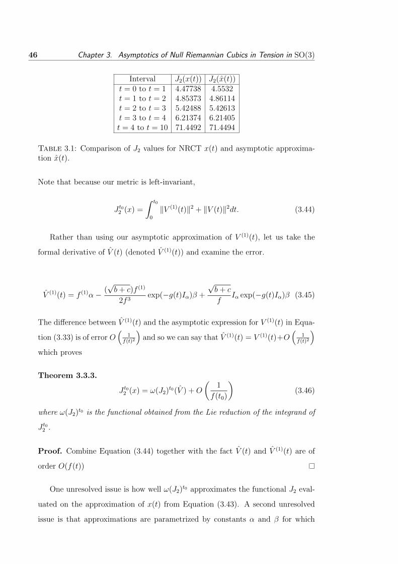
Interval J2(x(t)) J2(x(t))t = 0 to t = 1 4.47738 4.5532t = 1 to t = 2 4.85373 4.86114t = 2 to t = 3 5.42488 5.42613t = 3 to t = 4 6.21374 6.21405t = 4 to t = 10 71.4492 71.4494

Table 3.1: Comparison of J2 values for NRCT x(t) and asymptotic approxima-tion x(t).

Note that because our metric is left-invariant,

J t02 (x) =

∫ t0

0

‖V (1)(t)‖2 + ‖V (t)‖2dt. (3.44)

Rather than using our asymptotic approximation of V (1)(t), let us take the

formal derivative of V (t) (denoted V (1)(t)) and examine the error.

V (1)(t) = f (1)α− (√b+ c)f (1)

2f 3exp(−g(t)Iα)β +

√b+ c

fIα exp(−g(t)Iα)β (3.45)

The difference between V (1)(t) and the asymptotic expression for V (1)(t) in Equa-

tion (3.33) is of error O(

1f(t)2

)and so we can say that V (1)(t) = V (1)(t)+O

(1

f(t)2

)which proves

Theorem 3.3.3.

J t02 (x) = ω(J2)t0(V ) +O

(1

f(t0)

)(3.46)

where ω(J2)t0 is the functional obtained from the Lie reduction of the integrand of

J t02 .

Proof. Combine Equation (3.44) together with the fact V (t) and V (1)(t) are of

order O(f(t))

One unresolved issue is how well ω(J2)t0 approximates the functional J2 eval-

uated on the approximation of x(t) from Equation (3.43). A second unresolved

issue is that approximations are parametrized by constants α and β for which

3.4. Conclusion 47

there is no known way of computing from the initial conditions or vice versa. If it

could be shown the asymptotic formula produce a J2 which closely approximates

a real NRCT for small t too, then we may consider using them for interpolants

rather than x(t).

When x(t0) is known for some large t0 as well as the initial conditions, we

can estimate α and β by solving (with a numerical optimization package) the

non-linear over-constrained system of equations obtained by rearranging Equation

(3.43):

exp(−Iαg(t0))

αT

βT

(β × α)T

≈ P (t0)−1 ·D(t0) · x(t0) (3.47)

where D(t) := diag(f(t),√b+ c, f(t)

√b+ c).

3.4 Conclusion

In summary, we have provided several reasons to study Riemannian cubics in

tension by drawing on a problem in constrained optimisation. We specialise to the

null case due to tractability of analysis and a comparison of this case to well studied

curves in Euclidean space. We focus on the case Q = SO(3) due to the abundance

of practical applications and derive asymptotic formulae for the solutions to null

Riemannian cubics in tension and the corresponding null Lie quadratics in tension.

We mention how the functional values of the approximations can be compared as

well as suggesting how asymptotic formulas may be used if the initial conditions

and final endpoint are known.

49CHAPTER 4

Prior fields

4.1 Introduction

Let Q be a complete Riemannian manifold that represents the possible con-

figuration states of some dynamical system. We may take several observations

of the system ξ0, . . . , ξN at times t1, . . . , tN and we are interested in interpolating

the behaviour of the system in between. The dynamics of the system are often

approximated by a model such as a first order differential equation (representable

by a prior vector field A)

x(1)(t) ≈ A(x(t))

or possibly higher order differentiable equation such as a particle in a potential

field

∇tx(1) ≈ A(x(t))

More often than not, models of dynamical systems make simplifying assumptions

and so the observed data may not be representable exactly by a solution of the

model. We overcome this obstacle by searching for interpolants that best fit the

given model while agreeing with what is observed.

4.2 First order systems

For first order systems, Noakes in [26] introduces one such interpolant which

is a C1 curve x(t) such that x(ti) = ξi for i = 1, . . . , N for which the functional

AJ1(x) :=

∫ 1

0

‖x(1)(t)−Ax(t)‖2dt (4.1)

is minimised. A critical point of AJ1 is called a conditional extremal with prior

field A. If we restrict our problem to the case where N = 1, we can analyse the

constituent curves that make up such an interpolant. In the case that A = 0,

critical points of AJ1 would be the geodesics of the manifold and this framework

would produce geodesic interpolation.

50 Chapter 4. Prior fields

Example 4.2.1. Consider the vector field A(q) = q in Rn and we observe x(0) =

ξ0 and x(1) = ξ1. Then AJ1(x) =

∫ 1

0

‖x(1)(t) − x(t)‖2dt. The Euler-Lagrange

equations for this system are (x(2) − x(1)) + (x(1) − x) = 0. The conditional

extremals have the form x(t) = c1et+ c2e

−t where c1 = eξ1−ξ0e2−1

and c2 = ξ0 + ξ0−eξ1e2−1

.

Suppose x(t) is a conditional extremal and that we have a smooth one param-

eter family of variations xh(t) where x0(t) = x(t) and the endpoints are fixed. Set

Wh(t) := ∂xh∂h

. We can compute the derivative of AJ1 with respect to h:

1

2

∂AJ1(xh)

∂h=

∫ 1

0

〈∇h(x(1) −A), x(1) −A〉dt =

∫ 1

0

〈∇tWh −∇hA, x(1) −A〉dt

=

∫ 1

0

−〈Wh,∇t(x(1) −A)〉 − 〈∇hA, x(1) −A〉dt

where the last step uses integration by parts and the fact Wh(0) = Wh(1) = 0.

An important definition we will need to simplify this further is of the function Φ

defined by

〈ΦXY ,Z〉 := 〈∇ZY ,X〉. (4.2)

This is well defined since the metric is non-degenerate and because ∇XY is tenso-

rial in X . Here we interpret ∇Y as a linear operator with ΦY as its adjoint. This

construction allows us to isolate W (t) to one side of the inner product leaving:

1

2

∂AJ1(xh)

∂h= −

∫ 1

0

〈Wh,∇t(x(1) −A) + Φx(1)−AA〉dt.

Evaluating at h = 0, the fundamental lemma of calculus of variations gives us the

Euler Lagrange equations for conditional extremals

∇t(x(1) − A) + Φx(1)−AA = 0. (4.3)

For practical considerations, we are often interested in finding when the con-

ditional extremals minimise AJ1. An analysis requires higher order derivatives

of AJ1. For this, consider a two parameter family of variations of x(t) given by

xh1,h2(t) where xh1,h2(t) = x(t) when h1 = h2 = 0, and the endpoints are fixed.

4.2. First order systems 51

Defining W1 and W2 as the partial derivatives of xh1,h2 with respect to h1 and h2

respectively, the Hessian of AJ1 at the critical point is given by

∂AJ1(xh1,h2)

∂h2∂h1

=−∫ 1

0

〈W1,∇h2

(∇t(x

(1) −A) + Φx(1)−AA)〉dt

+(〈∇h2W1, x

(1) −A〉+ 〈W1,∇h2(x(1) − A)〉

)∣∣t=1

t=0(4.4)

This is calculated in a similar way to the Euler-Lagrange equations but we now

keep the boundary terms, differentiate a second time and substitute in the Euler-

Lagrange equations. Using the right hand entry of the inner product inside the

integral in (4.4), we define an A-Jacobi field as a vector field W (t) along a condi-

tional extremal x satisfying

∇W

(∇t(x

(1) −A) + Φx(1)−AA)

= 0. (4.5)

This says W to first order accuracy preserves the Euler-Lagrange equations but

only makes sense when we have a variation xh(t) already defined. We usually have

no variation to begin with but instead would like to be able to find to first order

accuracy a variation of x(t) for which Euler-Lagrange equations hold. This means

we need a differential equation for W (t) which does not require differentiation of

x(1) in the W (t) direction because we no longer have a variation xh(t) in mind.

The following theorem can be taken as the definition of A-Jacobi fields:

Theorem 4.2.2. The A-Jacobi field equation can be re-expressed as

∇2tW −∇t∇WA+R(W,x(1))(x(1) −A)+

R(A, x(1))W + Φx(1)−A∇WA+ Φ∇tW−∇WAA− ΦΦx(1)−AA

W = 0.(4.6)

When A = 0, this results in the usual Jacobi field equations for geodesics:

∇2tW +R(W,x(1))x(1) = 0.

Proof. To shorten the proof, we first make the substitution Y = x(1) −A. Then


we have

∇W (∇tY + ΦYA) = ∇t∇WY +R(W,x(1))Y +∇WΦYA.

The first term in this expression can be rewritten as ∇2tW −∇t∇WA. To simplify

the last term, we take its inner product with an arbitrary vector field X and also

extend W to a vector field W defined over the whole manifold. Because the inner

product will be tensorial in both W and X , we may assume that [W ,X ] = 0.

〈∇WΦYA,X〉 =W〈ΦYA,X〉 − 〈ΦYA,∇WX〉

=W〈∇XA, Y 〉 − 〈ΦYA,∇XW〉

=〈∇W∇XA, Y 〉+ 〈∇XA,∇WY 〉 − 〈ΦΦY AW ,X〉

=〈∇X∇WA+R(W ,X )A, Y 〉+ 〈Φ∇WYA,X〉 − 〈ΦΦY AW ,X〉

=〈ΦY∇WA+R(A, Y )W + Φ∇WYA− ΦΦY AW ,X〉

Since X can be taken to have any value at a given point, we must have equality

for the the left hand terms in the inner product. Finally, replacing ∇WY by

∇tW −∇WA and using the fact that R(A,A)W = 0 proves the result.

Two points x(t0) and x(t1) on a conditional extremal are said to be conjugate if

there is a non-trivial A-Jacobi field W (t) along x(t) such that W (t0) = W (t1) = 0.

Two general points q0, q1 ∈ Q are A-conjugate if they are conjugate along some

conditional extremal. Schrader and Noakes in [40] prove that AJ1 satisfies the

Palais-Smale condition on the space of absolutely continuous curves joining two

submanifolds of Q to show the existence of extremals in any homotopy class and

also prove that the conjugate points along any curve are isolated. Some stronger

results can be obtained if we now restrict ourselves to the case that Q is a bi-

invariant Lie groupG andA a left-invariant vector field1. Recall that a bi-invariant

1The requirement A be left-invariant is not necessary to do the Lie reduction but the equa-tions are rather complicated even in somewhat simple cases and lie outside the scope of thisthesis


Lie group satisfies 〈[u, v], w〉 = 〈u, [v, w]〉 for all u, v, w ∈ TgG. Let v ∈ TgG, recall

that the left Lie reduction L of v is given by L(v) := (dLg−1) v ∈ TeG. Then

for any vector field W (t) along a curve x(t), we can define a curve in the Lie

algebra by W (t) := L(W (x(t)). In the case W (t) = x(1)(t), we give the curve

W (t) = L(x(1)(t)) the name V (t).

Example 4.2.3. Suppose we have an object that we wish to rotate about its

centre of mass at a given fixed angular velocity Ω0 for a specified amount of

time. The state of a rigid body in absolute coordinates can be described by a

curve x(t) in SO(3), a bi-invariant Lie group. The angular velocity is defined

as Ω(t) = x(t)−1x(1)(t). We are able to take some measurements of the body’s

orientation in its motion and we find that the rotation of the object is not exactly

as specified. We may like to interpolate the object’s orientation between the

observations to display how it actually rotates over time. If it is the case that

we expect on average the angular velocity to be Ω0, then it is sensible to choose

an interpolant that minimises the mean square error between the body’s angular

velocity and Ω0.

The rotating mechanism attempts to keep Ω(t) a constant Ω0. This is to

say that we try to keep x(1) approximately A = x(t)Ω0 which is a left-invariant

vector field on SO(3). One such choice for an interpolating curve x(t) is one

that minimises AJ1. Trouble can arise when interpolating optimally as the ob-

served orientations become further apart. As with interpolating using piecewise

geodesics, if a conditional extremal interpolant contains an A-conjugate point, it

means we have not produced an optimal interpolant as the Hessian will not be

positive definite [18].

We will employ the use of a Lie reduction to simplify the equations obtained

for conditional extremals and their A-Jacobi fields. In doing so, it is important

to see how to calculate the Lie reductions for the various terms involved in these

equations. Let Ei be a basis for the left-invariant vector fields of G and let X ,Y

and Z be vector fields on G. Define smooth functions X, Y, Z : G→ Rn such that


Xg = X i(g)(Ei)g, Yg = Y j(g)(Ej)g and Zg = Zk(g)(Ek)g. We can then identify

X(g), Y (g), Z(g) as the Lie reduction represented in the chosen basis by seeing

that L(Xg) = X i(g)(Ei)e and so on. Then for covariant differentiation, omitting

the auxiliary variable g, we have:

L(∇XY) = L(∇XiEi(YjEj)) = L((EiY j) ·X iEj +X iY j∇EiEj)

= dY ·X +1

2[X, Y ].

where dY and X are thought of as elements of GL(g) and g respectively repre-

sented in the chosen basis. In the case that X is x(1) along some curve x(t), we

have

L(∇tY) = V (1)(t) +1

2[V, Y ]. (4.7)

Lie reduction of the curvature tensor is similarly calculated:

L(R(X ,Y)Z) = L(R(X iEi, Y jEj)(ZkEk)) = L(X iY jZkR(Ei, Ej)Ek)

=1

4[Z, [X, Y ]]. (4.8)

Lastly, we also would like to be able to calculate the Lie reduction of the adjoint

of the covariant differential, ΦXY . To compute this, we must first take the inner

product with an arbitrary vector field Z and use the non-degeneracy of the metric.

〈L(ΦXY),L(Z)〉 = L(〈ΦXY ,Z〉) = L(〈∇ZY ,X〉)

= 〈L(∇ZY), X〉 = 〈dY · Z +1

2[Z, Y ], X〉

= 〈dY ∗ ·X +1

2[Y,X], Z〉

where dY ∗ represents the adjoint with respect to the inner product. Because Z

was arbitrary, this means that

L(ΦXY) = dY ∗ ·X − 1

2[X, Y ]. (4.9)


In the setting of a bi-invariant group with left-invariant vector field A, Noakes

in [26] uses the Lie reduction to reduce Equation (4.3) to a much simpler equation

in the Lie algebra. Recall that since A is left-invariant, we can represent it by

A = Ae.

Theorem 4.2.4 (Noakes [26]). Let x(t) be a conditional extremal. Then V (t) =

L(x(1)(t)) satisfies

V (1) = [V,A] (4.10)

Proof.

∇t(x(1) − A) + Φx(1)−AA = 0 ⇐⇒ L(∇t(x

(1) − A) + Φx(1)−AA) = 0

⇐⇒ V (1) +1

2[V, V − A] +

1

2[A, V − A] = 0 ⇐⇒ V (1) + [A, V ] = 0

Using this new equation, Noakes[26] calculates the explicit solution of such

A-extremals given by the following theorem

Theorem 4.2.5 (Noakes [26]). Let x : [0, 1] → G be a conditional extremal with

A left-invariant (with A = Ae) and x(0) = e. Then x(t) can be written explicitly

in the form

x(t) = e(V (0)−A)teAt. (4.11)

Proof. The proof we give is for matrix Lie groups although Noakes proves it

more generally. Solving for (4.10) using an integration factor tells us that V (t) =

e−AtV (0)eAt. Using the linking equation x(1)(t) = x(t)V (t), we see that

x(1)(t)e−At = x(t)e−AtV (0). (4.12)

Using this and the product rule, we see that

d

dt(x(t)e−At) = (x(t)e−At)(V (0)− A). (4.13)


This is a differential equation for x(t)e−At which has the solution x(t)e−At =

e(V (0)−A)t and then multiplying both sides of the equation by eAt proves the result.

In the study of conjugate points along A-extremals, these extremals on Lie

groups were the first place to consider looking for examples. The following theorem

says that in bi-invariant Lie groups, solving conjugate points of prior fields for left-

invariant A correspond precisely to solving conjugate points for geodesics.

Theorem 4.2.6. Let x(t) : [0, 1] → G be a conditional extremal with A left-

invariant, x(0) = e. Then x(1) is an A-conjugate point if any only if expe V (0)− A

is a regular conjugate point of the geodesic expe (V (0)− A)t.

Proof. By Theorem 4.2.5, all A-extremals take the form et(V (0)−A)etA where V (0)

is variable. As etA does not change over different A-extremals, variations through

A-extremals correspond to variations through the left hand term et(V (0)−A). These

variations may fix the endpoints precisely when eV (0)−A is conjugate to e along

e(V0−A0)t

The proof of the above theorem means that for different choices of A on a

connected Lie group, we can have conjugate points placed anywhere. Figure 4.1

shows an example of conjugate points arbitrarily close together distance-wise in

S3

Although we have reduced the problem of finding conjugate points to a simpler,

more well studied problem, knowing about the A-Jacobi fields along has applica-

tions in interpolation. Solutions for A-Jacobi fields will let us answer questions

such as how sensitive a change in the endpoint velocities will be to a perturbation

of the initial conditions. We will now use the solutions for x(t) to find a differ-

ential equation for the Lie reduction of an A-Jacobi Field. In what will follow,

we will assume W (0) = 0 so we are only dealing with A-Jacobi fields that fix the

initial point. If V (0) = A, then we have a geodesic so we will also assume that

V (0) 6= 0.


Figure 4.1: Extremals on S3 ⊂ H with A = iπ and V (0) ≈ 0 (Stereographicprojection into R3).

Proposition 4.2.7. The A-Jacobi fields W (t) for which x(0) = e is fixed are

given by the series expression

W (t) =

(∞∑i=1

ti

i!T i−1(B)

)x(t) (4.14)

where T = ad(V (0)− A) and B = W (1)(0).

Proof. All variations will have up to first order the form xh(t) = e(V (0)+hB−A)teAt.

Then we explicitly calculate the formula W (t) = ∂xh∂h

∣∣h=0

using the formula [49] for

the derivative of the exponential map and it is easily verified thatB = W (1)(0).

A more easily understood formula can be obtained if instead of directly solving

variations of the solution, we study the effect of a variation on the underlying

differential equation. In effect we could now set A = 0 however we will preserve

it to see its effects in the process. In what will follow, we will effectively be

computing the derivative of the exponential but in a much simpler way than the

methods which exist in literature and has application to further chapters.

Theorem 4.2.8. Let x(t) be a conditional extremal and suppose W is the Lie


reduction of an A-Jacobi field. Then

W (2) + [V + A, W (1)] + [V, [A, W ]] = 0 (4.15)

Proof. Let xh be a variation through conditional extremals and let Vh be the

corresponding Lie reductions. Define Xh = dVhdh

. Differentiating the equation

V(1)h + [A, Vh] = 0 We can differentiate this equation with respect to h and we

have

X(1)h + [A,Xh] = 0 (4.16)

The relationship between W and Vh is that W (1) + [W , V ] = X (A proof of this

fact is in Chapter 5, page 86). Substituting, we get

W (2) + [V + A, W (1)] + [V (1), W ] + [A, [V, W ]] = 0

Using the fact that V (1) = [V,A] together with the Jacobi identity, we obtain

W (2) + [V + A, W (1)] + [V, [A, W ]] = 0

Before we explicitly solve this equation, we make some observations. Define

an operator which we will call the Lax operator defined by LC = ddt

+ adC . So

for example, LCV := V (1) + [C, V ]. Under this new definition, we see that the

condition for V to be a conditional extremal can be written as LAV = 0. The

condition for a vector field to be an A-Jacobi field was calculated by expanding

LVLAW = 0. The following proposition is an interesting property of conditional

extremals.

Proposition 4.2.9. Let x(t) an A-extremal. Then LVLA = LALV .

Proof. For any curve B in the Lie algebra, LALVB = LA(B(1) + [V,B]) = B(2) +

[V (1), B] + [V,B(1)] + [A,B(1) + [V,B]]. Using the fact V is an A-extremal, this is

equal to B(2) +[[V,A], B]+[V +A,B(1)]+[A, [V,B]]. Applying the Jacobi identity,


we are left with B(2) + [B(1), V + A] + [V, [A,B]] which we have already seen is

LVLAB.

The following propositions list some identities relating to the geometry of W .

Proposition 4.2.10. There exists a constant b1 ∈ R such that for all t,

〈W (1) + [V, W ], A〉 = b1. (4.17)

Proof. Taking inner products of (4.15) withA, we find: 〈W (2), A〉+〈[V, W (1)], A〉+

〈[V (1), W ], A〉 = 0 which implies ddt

(〈W (1), A〉+ 〈[V, W ], A〉

)= 0. Integrating

proves the result.


〈W (1) + [V, W ], V 〉 = 〈W (1), V 〉 = b2. (4.18)

Proof. Taking inner products of (4.15) with V , we find:

〈W (2), V 〉+ 〈[A, W (1)], V 〉 = 0 which implies〈W (2), V 〉+ 〈W (1), V (1)〉 = 0.


〈W (1) + [V, W ], V (1)〉 = b3 (4.19)

Proof. Taking inner products of (4.15) with V (1), we find:

〈W (2), V (1)〉+ 〈[V + A, W (1)], V (1)〉+ 〈[A, [V, W ]], V (1)〉 = 0 which implies

〈W (2), V (1)〉+ 〈[V, W (1)], V (1)〉+ 〈W (1), [V (1), A]〉+ 〈[V, W ], [V (1), A]〉 = 0 and so

〈W (2) + [V, W (1)], V (1)〉+ 〈W (1) + [V, W ], V (2)〉 = 0.


〈W , V − A〉 = (b2 − b1)t+ b4 (4.20)


Proof.

b2 − b1 = 〈W (1), V 〉 − 〈W (1) + [V, W ], A〉 = 〈W (1), V − A〉+ 〈W , V (1)〉 (4.21)

Integrating proves the result

Proposition 4.2.14. For conjugate points to exist, b1 = b2 and 〈W , V − A〉 = 0

Proof. In the case of Proposition 4.2.13, we choose our A-Jacobi fields to vanish

initially so the constant b4 = 0. This means for there to be conjugate points, we

must have b1 = b2 otherwise 〈W , V − A〉 would only be 0 at t = 0.

If X is a solution to LAX = 0, then X has the form X(t) = Ad(e−tA)X(0).

We know V is also a solution to LAV = 0 so V (t) = Ad(e−tA)V (0). Let us then

solve equations of the form LV W = X for W . Since we choose W (0) = 0, we

know that X(0) = W (1)(0).

W (1) + [V, W ] = Ad(e−tA)W (1)(0) (4.22)

Applying Ad(etA) to both sides, we find due to Ad invariance of ad that

Ad(etA)W (1) + [V (0),Ad(etA)W ] = W (1)(0) (4.23)

Defining Y (t) = Ad(etA)W (t), then Y (1)(t) = [A,Ad(etA)W ] + Ad(etA)W (1) and

Y (1) + [V (0)− A, Y ] = W (1)(0)

This is just a constant coefficient linear system. Because G is bi-invariant,

T = adV (0)−A is skew-adjoint and so imT ⊕ kerT = g, and that T : imT → imT

is an isomorphism. By setting Y = ν1 + ν2t with ν1 ∈ imT and ν2 ∈ kerT , there

is a unique solution for ν1 and ν2 such that T (ν1) + ν2 = W (1)(0). This leads to

the general solution Y = ν1 + ν2t− Ad(e−(V (0)−A)t)ν1 since Y (0) = 0 and implies

the following theorem


Theorem 4.2.15. If x(t) is an A-extremal on a Lie group and W (t) is the Lie

reduction of an A-Jacobi field W (t) which fixes the initial point x(0) = e, then

W (t) has the form:

W (t) = Ad(e−tA)(ν2t+ (1− Ad(e−(V (0)−A)t))ν1) (4.24)

where W (1)(0) = ν1 + ν2 and ν1 ∈ imT and ν2 ∈ kerT . Moreover, W (t) =

x(t)W (t) has the form:

W (t) = e(V (0)−A)t(ν2t+ (1− Ad(e−(V (0)−A)t))ν1)eAt (4.25)

Example 4.2.16. Let G be the algebra of unit quaternions in H thought of

as S3. Let A0 = (0, 1, 0, 0) and V (0) = (0, 4, 0, 4). The map T = adV (0)−A

on the Lie algebra has kerT = span(1,−1, 0) and imT = kerT⊥. Then we

see that W (t) = Ad(e−tA)(ν1 + ν2t − Ad(e−(V (0)−A)t)ν1) which has a zero when

ν1+ν2t−Ad(e−(V (0)−A)t)ν1 = 0. This example relates very closely to the motivating

example of a rotating body, but we choose S3 for a simpler description. S3 is

in fact just a a double cover of SO(3) with isomorphic Lie algebras. To see

that their Lie algebras are isomorphic, recall firstly that we already have a Lie

algebra isomorphism between so(3) and E3. Take the linear map between T1S3

and E3 given by the maps i 7→ 2e1, j 7→ 2e2, k 7→ 2e3. Then, as an example,

[12i, 1

2j] = (1

2i)(1

2j) − (1

2j)(1

2i) = 1

2k while we also have e1 × e2 = e3. This

calculation can be repeated with a more general vector to prove that this map is

an isomorphism.

In this example,

x(t) = (cos t cos 5t−3

5sin t sin 5t, cos 5t sin t+

3

5cos t sin 5t,

4

5sin t sin 5t,

4

5cos t sin 5t)

A possible Lie reduced A-Jacobi field would be

W (t) =(− 4 + 4 cos 10t, 3 sin 2t− sin 8t− 4 sin 12t, 3 cos 2t+ cos 8t− 4 cos 12t

)


If ν2 6= 0, then this equation cannot have any non-trivial zeros as both ν1 and

Ad(e−(V (0)−A)t)ν1 will be orthogonal to ν2. If ν2 = 0 on the other hand, the only

non-trivial zeros occur when Ad(e−(V (0)−A)t) = e which is when t = kπ‖V (0)−A‖ for

k ∈ N.

To see how such variations look, the first root of W (t) is t0 = π5. Here W (1)(0)

can be chosen anywhere in the space perpendicular to (3, 0, 4). We can see the

conjugate points by taking small perturbations to V (0) of the form V (0)+εW (1)(0)

for small ε.-2

-1

0

1

0

1

2

3

0.0

0.5

1.0

1.5

Figure 4.2: Perturbations of the initial condition V (0) (V (0) represented bythe red curve) in Example 4.2.16 for A-extremals with t ∈ [0, π

5]. Stereographic

projection of S3 onto R3 is used to represent the curves.

Example 4.2.17. Let us now consider the Lie group SL(2,R), the group of 2

by 2 real matrices with determinant 1. The Killing form [11] here is not positive

definite so this example no longer relates to the minimisation problem posed at the

beginning of the chapter however critical points can be calculated just the same

and the same formula for W (t) holds. Let A =

1 0

0 −1

and V0 =

1 −1

1 −1

.


Then x(t) =

et cos t −e−t sin t

et sin t e−t cos t

. Suppose W (1)(0) =

0 2

2 0

. Then ν1 = 1 0

0 −1

and ν2 = 0. We can then solve W (t) =

2e−t sin2 t e−t sin 2t

et sin 2t −2et sin2 t

.

By noticing the the conjugate points occur when t is a multiple of 2kπ, we can

find a point conjugate to the identity is

e2π 0

0 e−2π

.

4.2.1 Variable left-invariant priors It is easy to imagine interpolation

applications where the vector field may be modelled to be left-invariant but it is

not known which vector field to use. Consider now the system where we have an

unknown left-invariant prior field A and suppose now we let t go from [0, T ]. The

resulting Euler Lagrange equations for the system will be the same of that of the

fixed left-invariant prior field however an extra condition will come about when

differentiating the functional AJ1 with respect to A. Suppose As = A + sB with

B also left-invariant (represented as A and B in g).

As we are dealing with a bi-invariant metric, we can reduce the functional to:

AJ1(xh,s) =

∫ T

0

〈V (1)r −As, V (1)

r −As〉dt (4.26)

Differentiating this expression with respect to s, we get:

1

2

∂

∂sAJ1(xr,s)

∣∣s=0

=

∫ T

0

〈 dds

∣∣s=0As, V (1)

r −As〉dt

= 〈B, V (T )− V (0)− TA〉

If this is to equal 0 for all variations B of A, then it is clear that A = 1T

(V (T )−

V (0)). This shows that if A is to be estimated from the data as well, the best

choice to use is the average velocity between the points. The analysis then remains

the same as when A is known.


4.3 Second order systems

Usually in mechanics where forces and accelerations are involved, the dynamics

are governed by a second order system. Let L : (TQ⊕QTQ)×R→ R be a smooth

function and let x : [0, 1]→ Q be a C2 curve with known endpoints x(0) = q0 and

x(1) = q1. Let ν be a lifting of the curve x given by ν(x) = (x,∇tx(1), x(1)) and

define:

J(x) =

∫ 1

0

L(ν(x)(t), t)dt

Let A = (A1,A2) be a section of TQ⊕Q TM , and L(X, t) = 〈X −AX , X −AX〉

where the inner product is given by a general orthogonal relationship

〈(A1,A2), (B1,B2)〉 = 〈A1,B1〉+ λ〈A2,B2〉. Define

AJλ2 (x) :=

∫ 1

0

‖∇tx(1) −A1‖2 + λ‖x(1) −A2‖2dt (4.27)

This functional generalises that of Riemannian cubics in tension. We can of course

compute the Euler-Lagrange equations for AJλ2 although we may as well suppose

λ = 0 since we have studied that case in the first section of this chapter and

therefore we will write A1 as A. Let xh be a variation of x for which all of

x(1)(0) = x(1)(1) = ∇tx(1)(0) = ∇tx

(1)(1) = 0

1

2

dAJ02 (xh)

dh=

∫ 1

0

〈∇h(∇tx(1) −A1),∇tx

(1) −A〉dt

=

∫ 1

0

〈∇t∇hx(1) +R(

dxhdh

, x(1))x(1) −∇hA,∇tx(1) −A〉

=

∫ 1

0

〈∇2t

dxhdh

+R(dxhdh

, x(1))x(1) −∇hA,∇tx(1) −A〉

=

∫ 1

0

〈dxhdh

,∇3tx

(1) −∇2tA+R(∇tx

(1) −A, x(1))x(1) − Φ∇tx(1)−AA〉dt

Theorem 4.3.1. Let x(t) be a critical point of the functional AJ2 as defined in

Equation (4.27) with λ = 0. Setting Y (t) = ∇tx(1) −A, we see that x(t) satisfies

∇2tY +R(Y, x(1))x(1) − ΦYA = 0 (4.28)

4.3. Second order systems 65

Compare this result with the equation for first order conditional extremals

which when we set Y (t) = x(1) −A, get the equation ∇tY + ΦYA = 0. Secondly,

notice that every term in the expression involves A. If the manifold and vector

field displays symmetry in the form of Q being a bi-invariant Lie group and A

being left-invariant, then an interesting phenomenon occurs. In what will follow,

let Q be a Lie group G and A a left-invariant vector field. As for the first order

conditional extremals, we can carry out the Lie reduction on the Euler Lagrange

equations to examine the equation for V (t).

Theorem 4.3.2. The Lie reduction V (t) of an extremal of AJ02 defined in Equa-

tion (4.27) on a bi-invariant Lie group with A left-invariant satisfies

V (3) + [V, V (2)] = 0 (4.29)

Proof. Setting Y (t) = L(Y (t)), we have:

L(∇2tY +R(Y, x(1))x(1) − ΦYA

)=

(Y (2) +

1

2[V (1), Y ] +

1

2[V, Y (1)] +

1

2[V, Y (1) + [V, Y ]]

)+

(1

4[V, [Y , V ]]

)+

(1

2[Y , A]

)= Y (2) +

1

2[V (1) − A, Y ] + [V, Y (1)] = Y (2) + [V, Y (1)]

= V (3) + [V, V (2)].

This theorem is rather intriguing because A does not show up in the equation

for V (t) at all showing that the left invariance of the vector field produces no

local effect on the solutions. Interestingly, the Lie reduced equation obtained for

second order systems is identical to that of Lie quadratics and so the second order

conditional extremals on a Lie group are Riemannian cubics. The Euler Lagrange

equations don’t show the entire picture however and removing constraints on the

end-point velocities adds boundary conditions that are affected by A. The effects


of such boundary conditions are discussed in Chapter 5.

4.4 Time varying systems

We wish to extend the constructions of the previous sections to those where

the prior vector field Amay change with time. Many models of dynamical systems

are time dependent and so we might like to model the systems behaviour by an

equation such as x(1)(t) ≈ A(x(t), t). As before, we would like to find critical

points of the functional:

A(t)J1(x) :=

∫ 1

0

‖x(1)(t)−A(x(t), t)‖2dt (4.30)

over C1 curves x(t). As A is no longer strictly a vector field over the integration,

we must first extend the domain to describe the problem in a form we are more

familiar with. We do this by transforming the problem to the problem on the

product manifold Q× [0, 1] and restricting variations of the curve to those which

do not change the second parameter. In this manifold, A(x, t) = (A(x, t), 1) is

now a smooth vector field (where A(x, t) is the original pseudo-vector field).

Let x : [0, 1]× (−ε, ε)→ Q× [0, 1] define a variation of curves x(t, h) such that

x(t, 0) is a critical point and moreover we will restrict ourselves to those variations

for which π2x(h, t) = t. Set Wh,t =∂xh,t∂h

and Xh,t =∂xh,t∂t

so as to avoid confusion

regarding the ∇t notation.

1

2

∂A(t)J1(xh,t)

∂h=

∫ 1

0

〈∇W (X −A), X −A〉dt

=

∫ 1

0

〈∇XW −∇WA, X −A〉dt

=

∫ 1

0

−〈W,∇X(X −A)〉 − 〈∇WA, x(1) −A〉dt

=

∫ 1

0

−〈W,∇X(X −A) + ΦX−AA〉dt

Up to this point, nothing is different to time invariant systems. The difference

arises because our W is restricted purely to variations that do not change the

4.4. Time varying systems 67

second argument and we can only conclude that the projection of ∇X(X −A) +

ΦX−AA into TQ is 0. In order to calculate this projection, we must first compute

the connection on a product manifold Q1 ×Q2.

Let (u1(x), . . . , un1(x), v−1(y), . . . , v−n2(y)) be local coordinates for a chart on

Q1 × Q2 using an atlas of cartesian products of atlases on Q1 and Q2. Indices i

and j are similar if they have the same sign, denoted i ' j. By definition of the

metric, gij = 0 whenever i 6' j. The formula for the Levi-Civita connection is

given by ∇U i∂iVj∂j = (U i ∂V k

∂i+ U iV jΓki,j)∂k where Γki,j is defined by 1

2gkr(∂igrj +

∂jgir−∂rgij). When i, j, and k are similar, Γki,j is known since gkr is only ever non-

zero for k ' r. Because of symmetry, there are only two other cases to examine:

When i ' j 6' k and i ' k 6' j. Because the only terms that contribute are when

r ' k, it can be seen that Γki,j = 0 in both the above cases. We can then define

the covariant derivative as follows:

∇(U1,U2)(V1,V2) = (∇Q1

U1 V1 + dV1(U2),∇Q2

U2 V2 + dV2(U1)) (4.31)

where ∇Q1 and ∇Q2 are connections on Q1 and Q2. The partial derivative terms

dV1(U2) and dV2(U1) are defined because the tangent space remains fixed in the

orthogonal direction. In the case of Q × R, we have the following for covariant

derivatives along x:

∇XA = (∇QXA+ d2A,0) (4.32)

∇XX = (∇QXx

(1),0) (4.33)

where d2 refers to differentiation with respect to the second coordinate of A.

Under this computation, we obtain the Euler-Lagrange equations with the original

connection on Q.

Theorem 4.4.1. A solution x(t) to a critical point of A(t)J1 as defined in Equation

(4.30) satisfies

∇t(x(1) −A) + Φx(1)−AA−

∂A∂t

= 0. (4.34)


If Q is a bi-invariant Lie group G and A(g, t) = dLgA(e, t) =: A(t), then we

can compute the Lie reduction of the above equation. As the covariant derivatives

are partial in the X direction, the first two terms are treated the same as the Lie

reduction for ordinary prior fields on a Lie group. The last term on the other

hand is differentiated in the t direction.

Theorem 4.4.2. A critical point of J as defined in Equation (4.30) when there is

time-dependent left-invariant prior field A(t) on a bi-invariant Lie group satisfies:

V (1)(t)− A(1)(t) = [V (t), A(t)] (4.35)

Making the substitution Y (t) = V (t)−A(t), we obtain a nicer form of Theorem

4.4.2:

Y (1)(t) = [Y (t), A(t)] (4.36)

We have seen what solutions to this equation are when A(t) is constant. The

simplest case after A(t) being constant is if A(t) is linear. This is a useful practical

case to study to make because we can approximate more complicated vector fields

using line segments. If A(t) = A0 + A1t, then various scenarios can occur. If

[A0, A1] = 0, the solutions are Y (t) = Ad(e−(A0t+12A1t2))Y (0). These can be solved

for x(t) in the same manner as in the time-invariant case.

Proposition 4.4.3. Suppose x(t) is a conditional extremal for the time-variant

left-invariant prior field defined by A(t) = A0 + A1t where [A0, A1] = 0 and

x(0) = e. Set B(t) = A0t+ 12A1t

2. Then the solutions for x(t) are

x(t) = e(V (0)−A(0))teB(t) (4.37)

Proof. We have seen that Y (t) = Ad(e−B(t))Y (0) and so V (t) = Ad(e−B(t))(V (0)−

A(0)) + A(t) = Ad(e−B(t))(V (0) − A(0) + A(t)). Using the formula x(1)(t) =

x(t)V (t) and the product rule, we can see that

(x(t)e−B(t))(1) = x(1)(t)e−B(t) − x(t)e−B(t)A(t) =(x(t)e−B(t)

)(V (0)− A(0))


Therefore x(t)e−B(t) = e(V (0)−A(0))t and so x(t) = e(V (0)−A(0))teB(t)

We should note that this proof would work even if A(t) was more general so

long as A(t) is contained in a Lie subalgebra h with [h, h] = 0 in which case we

would set B(t) =∫A(t)dt. As seen by the above theorem and the discussion in

the proof of Theorem 4.2.6, the conjugate points of x(t) depend only on V (0) and

the constant term of A(t) which is quite curious. If on the other hand [A0, A1] 6=

0, then the solution becomes significantly more difficult to find. If we restrict

ourselves to the manifold SO(3), then solutions in this case can be solved up to a

single quadrature.

Theorem 4.4.4. Solutions to the equation for ∇X(X − A) − dAdt

+ ΦX−AA = 0

for A = A0 + A1t with [A0, A1] 6= 0 and X = x(1) can be solved exactly in terms

of a single quadrature when the Lie group is SO(3).

Proof. We have the equation Y (1)(t) = [A0 + A1t, Y (t)] = (adA0 + t adA1)Y (t)

where Y (t) = V (t) − A(t). Suppose g is a Lie Algebra such that ad g belongs in

the Lie algebra of some matrix subgroup G of GL(dim g,R). Then we can see

that when extending Y (t) to a fundamental matrix Ψ(t), we have an equation of

the form Ψ(1)(t) = (B0 + tB1)Ψ(t) where Ψ(t) ∈ G and B0, B1 ∈ TeG. Using

the duality [21] property of null Riemannian cubics, we see that the same Ψ(t)

satisfies Ψ(1)(t) = Ψ(t)C(t) where C(t) is a null Lie quadratic and so Ψ(t) is a null

Riemannian cubic. This shows that solutions to Y (t) correspond to projections

of a null Riemannian cubic in G. For example, consider g = E3 and ad g only

contains 3× 3 skew-symmetric matrices which are in the Lie algebra of SO(3,R).

Pauley in [30] finds the solutions of null Riemannian cubics in SL(2,C) implic-

itly in terms of special functions and then which can be transformed via a homo-

morphism into solutions for SO(3). Also within the paper are solutions for null

Lie quadratics and their first three derivatives. Let Y (t) be a projection of a null

Riemannian cubic Y (t) = xc(t) · C0, where C0 is chosen so that xc(0)C0 = Y (0).

Then V (t) = xc(t)C0 − A1t− A0 is known exactly.


For what is to follow, recall that we have a Lie algebra isomorphism B :

so(3) → E3 (denoted by B : D 7→ DE) defined by D · v = DE × v where we also

have the relationship AdgD = gDE due to the properties of orthogonal matrices

and the cross product. The result on duality [21] shows it is in fact possible to

reconstruct the A-extremal if we know the quantity Y (t). This is because we know

that ddt

Adx(t) Y (t) = Adx(t)(Y(1)(t)+[V, Y (t)]) = Adx(t)(V

(1)−A(1) +[V,−A]) = 0

and so Adx(t)Y (t) = D. Considering the vectors Y (t) and D as elements of E3, the

equation can be rewritten x(t)YE(t) = CE. We are then interested in the action

of x(t) in a vector orthogonal to YE(t). Y(1)E (t) is one such vector and it can be

solved knowing Y (t). Set W3(t) := YE(t)/‖YE(t)‖, W1(t) := Y(1)E (t)/‖Y (1)

E (t)‖ and

W2(t) := W3(t)×W1(t) and define:

θ(t) :=

∫ t

0

〈W1(s),W(1)2 (s) + VE(s)×W2(s)〉ds (4.38)

U(t) :=[

W1 cos θ(t) +W2 sin θ(t) W2 cos θ(t)−W1 sin θ(t) W3(t)]

(4.39)

Then x(t) = U(0)U(t)T is an A(t)-extremal. To prove this, we will show that

x(1)(t) = x(t)V (t). We can see first of all that W(1)3 = W3×VE because Y

(1)E = YE×

VE and as a consequence ‖YE‖ is constant. So U(1)3 = −VE × U3 = −V U3. Now,

using the fact that θ(1)(t) = 〈W1(t),W(1)2 (t) + VE(t)×W2(t)〉 and that W1,W2

and W3 are orthonormally related, we obtain:

〈U (1)1 ,W1〉 = −〈W1, VE ×W2〉 sin θ = −〈V U1,W1〉

〈U (1)1 ,W2〉 = 〈W1, VE ×W2〉 cos θ = −〈VE ×W1,W2〉 cos θ = −〈V U1,W2〉

〈U (1)1 ,W3〉 = 〈U (1)

1 , U3〉 = −〈U1, U(1)3 〉 = −〈U1,W3 × VE〉 = −〈V U1,W3〉

Therefore U(1)1 = −V U1 as they act identically on a basis for E3. Lastly, U

(1)2 =

−(VE × U3)× U1 − U3 × (VE × U1) = −VE × (U3 × U1) = −V U2. It is then seen

that U (1) = −V U . Then x(1)(t) = (U(0)U(t)T )(1) = −U(0)U(t)TV (t)T = x(t)V (t)


since V (t) is skew-symmetric.

4.4.1 Time varying prior fields for solvable A(t) in a bi-invariant Lie

group In some instances, A(t) may be a vector field for which integral curves are

already known. We now prove a remarkable fact that generalises many of the

previous results. If we know the integral curves of A(t), we can solve the equation

V (1)(t) − A(1)(t) = [V (t), A(t)] exactly and reconstruct the conditional extremal

up to a single quadrature.

Theorem 4.4.5. Let G be a bi-invariant Lie group and suppose that z(1)(t) =

z(t)A(t) where A(t) is a curve in the Lie algebra. Then we can solve V (t) and x(t)

exactly in terms of z(t), where x(1)(t) = x(t)V (t) and V (t) satisfies the equation

V (1)(t)− A(1)(t) = [V (t), A(t)].

Proof. We prove the result using the notation of matrix groups although we note

that the same line of proof holds for a general group. As before, set Y (t) =

V (t)− A(t) and without loss of generality, set z(0) = x(0) = e. The equation

d

dtAdz(t) Y (t) = Adz(t)(Y

(1)(t) + [A(t), Y (t)]) = 0 (4.40)

shows that Adz(t) Y (t) is constant and so

Y (t) = Adz(t)−1 Y (0) = z(t)−1Y (0)z(t). (4.41)

Substituting the definition of Y (t) gives us the following equation for V (t):

V (t) = z(t)−1(V (0)− A(0))z(t) + A(t). (4.42)

Pre-multiplying by x(t) and post-multiplying by z−1(t), we see that:

x(1)z−1 = xz−1(V (0)− A(0)) + xAz−1 (4.43)


Applying the product rule on (xz−1)(1), we obtain:

(xz−1)(1) = xz−1(V (0)− A(0)) + xAz−1 − xz−1z(1)z−1

= xz−1(V (0)− A(0)) + xAz−1 − xAz−1

= (xz−1)(V (0)− A(0)) (4.44)

and by solving the differential equation, we see that:

x(t) = e(V (0)−A(0))tz(t) (4.45)

This allows us to generate a whole family of solutions for when the prior vector

field is integrable. There are many examples for which the solutions for z(t) are

known.

• A(t) = At+B in SL(2,C) or SO(3) (Corresponding to z(t) being the inverse

of a null Riemannian cubic)

• A(t) being a null Lie quadratic in SL(2,C) or SO(3) (Corresponding to z(t)

being a null Riemannian cubic)

• A(t) is a multiple of a fixed vector. A(t) = f(t)A0 (z(t) is a reparameterised

geodesic)

• A(t) is a Jupp and Kent quadratic, as seen in [31, Chapter 4]

Notice that we now have two alternate ways of solving for Y (t) in the equation

Y (1)(t) = [A1t + A0, Y (t)]. One way relies on a special property of so(3) (where

the adjoint map on E3 converts to regular multiplication in the matrix group) to

convert the system into Ψ(1)(t) = (ad(A1)t+ ad(A0))Ψ(t). The second technique

is more general and can reduce solving a linked equation of the form x(1)(t) =

x(t)V (t) and V (1)(t) − A(1)(t) = [V (t), A(t)] into solving for integral curves of

A(t).


Suppose we now started with the equation V (1)(t) = [V (t), A(t)]. If we know

the solutions of z(1)(t) = z(t)A(t), we would indeed be able to solve for V (t) using

the same argument. We then however cannot easily construct a Lax pair and so

we do not have a known way of integrating V (t) to find x(t). This shows that the

form of the equation for V (t) is necessary for this theorem to work.

4.4.2 Time varying prior fields in SO(3) The method Pauley uses in [30]

to solve null Riemannian cubics in SL(2,C) are far more powerful than realised

in the paper. The same methods can be used to solve a much wider class of

differential equations. These additional solutions have applications in the case of

time dependent prior fields. We will borrow heavily from Pauley’s methods to

find solutions of interest.

What may well be the next simplest case after examining affine prior fields is

the case when A(t) is of the form A(t) = f(t)A1+A0 where [A1, A0] 6= 0. Recall the

Lie reduction equation for time varying prior fields says Y (1)(t) = ad(A(t))Y (t)

and so we can write Y (1)(t) = (f(t) ad(A1) + ad(A0))Y (t). Treating Y (t) as a

curve in E3, we extend the system to one involving the fundamental matrix Ψ(t),

we have that Ψ(1)(t) = (f(t) ad(A1) + ad(A0))Ψ(t) where ad(A1), ad(A0) ∈ so(3).

Because the factor of Ψ(t) is in TΨ(t) SO(3) and Ψ(0) = I3×3 ∈ SO(3), it must be

the case that Ψ(t) ∈ SO(3).

The equivalent problem in SL(2,C) is Ψ(1)(t) = (f(t)B1 + B0)Ψ(1)(t) where

B1, B0 ∈ su(2) are obtained by the usual Lie algebra isomorphism from so(3) into

the Pauli matrices.

Because the matrix B1 is skew-Hermitian, we can diagonalize it with a unitary

matrix and the diagonal matrix will be skew-Hermitian too. Moreover since f(t)

is arbitrary, we will assume B1 is the diagonal Pauli matrix D(i,−i) and that

the diagonal terms of B2 are 0. We may assume the off diagonal terms of B2 are

non-zero otherwise we can solve the system with an integrating factor.

p(1)1

p(1)2

=

f(t)

i 0

0 −i

+

0 z

−z 0

p1

p2

(4.46)


Writing out these equations, we have

p(1)1 = if(t)p1 + zp2 (4.47)

p(1)2 = −if(t)p2 − zp1 (4.48)

Differentiating (4.48) and substituting (4.47), we see that:

p(2)2 = −if (1)(t)p2 − if(t)p

(1)2 − z(if(t)p1 + zp2) (4.49)

Re-substituting (4.48) results in an equation with only p2 terms

p(2)2 = −if (1)(t)p2 − if(t)p

(1)2 + if(t)(if(t)p2 + p

(1)2 )− zzp2) (4.50)

Simplified, this says, p(2)2 +(zz+f(t)2+if (1)(t))p2 = 0. By making the substitution

g(t) = if(t), c2 = zz ≥ 0, and setting φ(t) := p2(t), we are left with the task of

solving the equation

φ(2)(t) + (c2 − g(t)2 + g(1)(t))φ(t) = 0 (4.51)

Many possible functions for g(t) lead to this system having known solutions.

Letting g(t) = 1t+t0

, we obtain solutions φ(t) = c1( cos(t)1+t

+sin(t))+c2( sin(t)1+t−cos(t)).

This g(t) although making the ODE particularly easy to solve also could represent

a situation where one vector fields effects are being damped over time. A more

realistic situation with damping which may happen in the real world would be

where we have a damping factor such as g(t) = e−γt. While the solution is not

straightforward, Mathematica shows it can be solved in terms of confluent hy-

pergeometric functions of the second kind and generalised Laguerre polynomials.

Once p2 is solved, p1 is found from 4.48. The original f(t) is easily recoverable

from the various simplifications that have been made and so we have completed

what we set out to do.

Now that we have solved for Ψ(t), we can apply the homomorphism of SU(2)


into SO(3) generated by the Lie algebra isomorphism and therefore produce a

solution for Ψ(t) in SO(3). Recall that this represents the fundamental matrix

of the solutions for Y (t) and therefore Y (t) = Ψ(t)Y (0) which means V (t) =

Ψ(t)Y (0) + A(t). Using the results on duality [21], we are then able to take this

solution and produce a solution in quadrature for the time invariant conditional

extremal x(t).

We wish to investigate which functions f(t) lead to a solvable system of equa-

tions. It is interesting to note there are two differential equations playing about

in Equation 4.51 for φ(t).

φ(2)(t) + q(t)φ(t) = 0 (4.52)

c2 − g(t)2 + g(1)(t) = q(t) (4.53)

The first of these is a second order linear ODE while the second is a first order

non-linear ODE. When one tries to solve these equations in a computer package

such as Mathematica, they find that solutions to (4.52) can be solved by the

software when and only when solutions to (4.53) can be solved and moreover, the

solutions are of a similar form. The family of equations given by (4.53) are a

subclass of a more general family known as non-linear Riccati equations [13].

One interesting property of the Riccati equation ([38]) is that once we know a

single solution, we can obtain the rest by quadrature.

Let g0(t) be a solution to (4.53), then the general class of solutions for (4.53)

is:

g(t) = y0(t) + Φ(t)

(C −

∫Φ(t)dt

)−1

where Φ(t) = exp(∫

2g0(t))

and C is an arbitrary constant.

If we make the substitution ψ(t) = exp(−∫g(t)

), we see that

ψ(2)(t) + (q(t)− c2)ψ(t) = 0

This is a linear second order differential equation and so we see the system of


equations we are in fact solving for are

φ(2)(t) + q(t)φ(t) = 0

ψ(2) + q(t)ψ(t) = c2ψ(t)

for some q(t). Another way of expressing this is that there is a differential operator

d2

dt2+ q(t) for which both 0 and c2 are eigenvalues. By setting q(t) = −V (t)

where V (t) is the negative of some potential function(the force), this operator

is the negative of the well known one dimensional time-independent Schrodinger

operator [42](also called the Hamilton operator) H = −∇2 +V (t) and if c2 = −E,

we obtain the Schrodinger equations Hψ = Eψ and Hψ = 0. That is, we are

after solutions to both a zero and a negative energy state. This also relates right

back to the discussion in section 3.1.1 in which we described q(t) = 0.


4.4.3 Second order time-variant systems A similar analysis can be

made for the functional

J2A(x) :=

∫ 1

0

‖∇tx(1) −A (x(t))‖2dt (4.54)

The Euler Lagrange equations are given by

∇2XZ +R(Z,X)X − φZA ⊥ TQ (4.55)

where Z = ∇XX − A. Recall that

∇XA = (∇QXA+

∂

∂tA, 0) (4.56)

∇XX = (∇QXX, 0) (4.57)

Moreover, because of the curvature tensor of R being 0 and the definition of the

product metric, R(X, Y )Z = RQ(π1X, π1Y )π1Z where π1 is projection onto the

first coordinate. To compute φZA, we have seen that on the product manifold

X × Y , that

∇(UX ,UY )(VX , VY ) = (∇XUXVX + dVX(UY ),∇Y

UYVY + dVY (UX))

This implies that

φ(UX ,UY )(VX , VY ) = (φXUXVX + dV TY (UY ), φYUY VY + dV T

X (UX))

Therefore φZA = (φZ1A, dAT (Z1)). Taking projections, we obtain the following

Euler Lagrange equations on Q:

Theorem 4.4.6. A critical point x(t) of the functional defined in Equation (4.54)

satisfies:

∇2XZ −

∂

∂t(∇XA)−∇X(

∂

∂tA)− ∂2

∂t2A+R(Z,X)X − φZA = 0 (4.58)


where X = x(1)(t)

Second order time varying systems on Lie groups

Suppose now the manifold Q is a bi-invariant Lie group G. In order to carry

out the Lie reduction, we need to only focus on the three terms with the partial

derivatives.

L (−∇XA) = −1

2

[V,∂A

∂t

]L(− ∂

∂t(∇XA)

)= −1

2

[V,∂A

∂t

]L(− ∂2

∂t2A

)= − ∂2

∂t2A

Combining this with the Lie reduction for the remaining equations to which we

already know the value, we obtain the theorem:

Theorem 4.4.7. Let x(t) be a critical point of (4.54) in a bi-invariant Lie group

with prior field A(t). Then the Lie reduction V (t) of x(t) satisfies

V (3)(t)− A(2)(t) + [V (t), V (2)(t)− A(1)(t)] = 0 (4.59)

This then explains why the time invariant prior fields reduced to the Rie-

mannian cubic equation. One substitution which can be made is if by setting

Y (t) := V (t)−∫ t

0A(s)ds, then Y (t) satisfies:

Y (3)(t) +

[Y (t) +

(∫ t

0

A(s)ds

), Y (2)(t)

]= 0 (4.60)

If we set Z(t) = V (2)(t) − A(1)(t), then we see that Z(1)(t) = [Z(t), V (t)] and so

(Z(t), V (t)) is a Lax pair.

Proposition 4.4.8. The Lie reduction V (t) of a critical point of 4.54 satisfies:

‖V (2)(t)− A(1)(t)‖ = c (4.61)

〈V (3)(t)− A(2)(t), V (t)〉 = 0 (4.62)

4.5. Conclusion 79

Proof. Take inner products of Equation (4.59) with V (2)(t) − A(1)(t) and V (t)

respectively and use the bi-invariance of the metric.

Corollary 4.4.9. If A(t) is a smooth function of t defined on all of R, then for

a fixed V (0), V (1)(0) and V (2)(0), V (t) extends to a unique C∞ solution of 4.59

also defined on all of R.

Proof. The constraint on V (3)(t) is smooth in all variables and so we have local

existence and uniqueness by the Picard-Lindelof theorem. A solution V (t) can

only fail to be indefinitely extended when any of V (t), V (1)(t) and V (2)(t) diverge

in finite time (See [47, Chapter 1]). Since A is smooth, on any interval [t0, t1], A

and its derivatives are bounded. Suppose then that ‖A(1)(t)‖ ≤ 2k − c. Then we

have from Equation (4.61) that ‖V (2)(t)‖ ≤ c+ ‖A(1)(t)‖ ≤ 2k. This also implies

that ‖V (1)(t)‖ ≤ 2kt+‖V (1)(0)‖ and ‖V (t)‖ ≤ kt2 +‖V (1)(0)‖t+‖V (0)‖ implying

none of V (t), V (1)(t) and V (2)(t) diverge in finite time.

Corollary 4.4.10. If G is compact, then there is a unique conditional extremal

x : R→ G satisfying x(0) = x0, x(1)(0) = v0, ∇tx(1)(0) = v1 and ∇2

tx(1)(0) = v2

Proof. Corollary 4.4.9 guarantees a solution for V (t) for all t ∈ R. Lemma 2.4

in [18] says that a smooth vector field with compact support has flows defined for

all t. Apply this lemma to the vector field V (x, t) = xV (t) defined on G× [t0, t1]

where t0 and t1 are arbitrary.

4.5 Conclusion

In summary, we have described A-Jacobi fields for first order prior fields and

have derived solutions and properties for A-Jacobi fields in the special case bi-

invariant Lie groups with a left-invariant prior field. We have shown that in

the case of an unknown left-invariant prior fields, that the average of the initial

and final velocities defines the optimal choice of prior field. For second order

prior fields, the Euler-Lagrange equations were derived in the case of a general

Riemannian manifold and the Lie reduced Euler-Lagrange equations in the case

of a bi-invariant Lie group with a left-invariant prior field were obtained. In the


latter case, somewhat surprisingly, the prior field does not appear in the equations

except as boundary conditions. We extend the concept of prior fields to those

which may vary with time for both first and second order conditional extremals

and extend the framework for handling this situation. Once specialising to the

Lie group setting, we are able to calculate solutions in a variety of situations

and mention an interesting connection to Riccati equations and the Schroedinger

equation. For second order time varying prior fields on a compact Lie group, we

prove the extendibility of solutions to all values of time.

We summarise the extremals considered so far and their corresponding func-

tionals (symbol and formula) with a table. Time varying versions refer to the

vector field A being a function of time as well as position in the manifold.

Name of extremals Symbol Functional

Geodesics J1

∫ 1

0‖x(1)‖2dt

Riemannian cubics J2

∫ 1

0‖∇tx

(1) −A‖2dt

Riemannian cubics in tension Jλ2∫ 1

0‖∇tx

(1) −A‖2dt+ λJ1

First order conditional extremals AJ1

∫ 1

0‖x(1) −A‖2dt

Second order conditional extremals AJλ2

∫ 1

0‖∇tx

(1) −A‖2dt+ λ(AJ1)

Table 4.1: List of various extremals with their corresponding functional’s symboland expression.

81CHAPTER 5

Linear interpolation schemes on bi-invariant Lie groups

5.1 Introduction

In the previous two chapters, we concerned ourselves with Riemannian cubics

in tension and conditional extrema in first and second order settings, as well as

non-autonomous first order systems. What remains to be discussed are algorithms

for interpolating efficiently and accurately. As we will see in this chapter, the

problem of interpolation requires the solving of an inherently coupled system

of boundary value problems. Even in the case for elastic curves in E2 where

the solution is completely known [15], their use in interpolation applications is

extremely limited due to the difficulty of satisfying nonlinear boundary value,

interior value and smoothness conditions. Polynomial splines are effective because

of their ability to reduce the system of equations to a linear system. Noakes in [27]

introduces a technique for interpolating data that falls near a geodesic by using

approximations to a natural Riemannian cubic spline. In this chapter, we give an

exposition of these ideas and how they apply to the case of second order conditional

extremals on a bi-invariant Lie group with A left-invariant. Moreover, we employ

a technique analogous to those of the traditional B-splines in Euclidean space to

reduce the problem of approximating a natural conditional extremal spline into a

solving a tridiagonal linear system.

Let Q be a smooth n-dimensional Riemannian manifold. A data list on Q is

an ordered (N + 1)-tuple

D = ((t0, ξ0), (t1, ξ1), . . . , (tN , ξN))

where 0 = t0 < t1 < · · · < tN = 1 and ξi ∈ Q for 0 ≤ i ≤ N .

Given a data list D, we say a curve x(t) is D-feasible if x(ti) = ξi for all

0 ≤ i ≤ N . Let D ⊂ ([0, 1] ×M)N+1 be a non-empty set of data lists, then an

interpolator is a Ck function I : D × [0, 1] → M such that xD(t) := I(D, t) is D

feasible for all D ∈ D. We say I is linear when given D, I(D, t) can be computed

82 Chapter 5. Linear interpolation schemes on bi-invariant Lie groups

by solving a system of linear equations. We are interested in producing a linear

interpolator which attempts to approximately minimise a variational problem.

Definition 5.1.1. Let R be an open neighbourhood of the 0-section in Γ(TQ).

A C∞ function E : R → Q, with all its derivatives bounded, is said to be quasi-

exponential when, for any q ∈ Q and any v ∈ TqQ,

E(q, 0) = q andd

dhE(q, hv)

∣∣∣∣h=0

= v (5.1)

The exponential map (on any complete Riemannian manifold) is quasiexpo-

nential although for the purpose of linear interpolation in SO(3), the following

map is preferable

Definition 5.1.2. The Cayley transform T : TSO(3) → SO(3) is given by the

formula

T (q, v) = q

(1 +L(v)

2

)(1− L(v)

2

)−1

(5.2)

where we recall that L(v) is the Lie reduction of v. The reason we will use the

Cayley transform is because calculating the inverse Cayley transform is performed

by solving a linear system of equations.

5.2 Second order prior fields in SO(3)

We will begin by studying interpolants minimising the functional relating to

second order time varying left-invariant prior fields in SO(3). First order prior

fields are only required to be piecewise C1 (for example, when A = 0, we have

piecewise geodesic interpolation) and therefore the boundary value problems as-

sociated with these are considerably simpler. Consider the functional J restricted

to D-feasible curves:

AJ2(x) =N−1∑i=1

∫ ti+1

ti

‖∇tx(1) −A(x(t))‖2dt (5.3)

Minimizers of this functional are known as natural second order conditional

splines. We are interested in constructing an interpolator which approximates

5.2. Second order prior fields in SO(3) 83

these splines and comes close to being a minimizer of AJ2.

Given a variation xh through piecewise extremals of AJ2 between any two

knots of this functional, if we differentiate with respect to h and ignore the terms

corresponding to the Euler Lagrange equations (which are 0 since we vary through

piecewise extremals), we are left with:

d

dh

∣∣∣∣h=0

AJ2(xh) =N−1∑i=1

[〈∇t

dxhdh

,∇tx(1)h −A〉 − 〈

dxhdh

,∇2tx

(1)h −∇tA〉

]∣∣∣∣ti+1

ti

(5.4)

After applying a Lie reduction, we see that:

d

dh

∣∣∣∣h=0

AJ2(xh) =N−1∑i=1

[〈W (1) +

1

2[V,W ], V (1) − A〉 − 〈W,V (2) +

1

2[V, V (1)]〉

]∣∣∣∣ti+1

ti

Because we can set W (1) arbitrarily and in such a way that its support only

contains one ti, we obtain the following equations:

V (1)(ti) = A(ti) (5.5)

V (1)(t−j )− A(t−j ) = V (1)(t+j )− A(t+j ) (5.6)

for all i ∈ 0, N and j /∈ 0, N.

Although we previously required x(t) be piecewise C2, we can relax conditions

on differentiability at the interior knots in a way so that the integral is still defined.

In order for this to occur, discrete approximations to∫ 1

0‖∇tx

(1) −A‖2 must not

be too large and so we require that x(t) be C1 at the knots. Even under this

restriction, we find that equation (5.6) imposes the condition optimal solutions be

C2.

Equations (5.6) and (5.5) together with the Euler-Lagrange Equations (4.58)

between any two knots give us all the necessary properties for critical points of

this interpolation problem and show that V must be continuously differentiable.

To find a critical point, we must piece together solutions of the Euler Lagrange

equations in such a way that, at the first and last knots, we have V (1) = A and


moreover we require V (1) to be continuous at the interior knots. While solving

explicitly for V is difficult, we may approximate V by taking a simple extremal

V0 which satisfies V(1)

0 (t) = A(t) everywhere (not necessarily interpolating the

interior data points), and then taking a Taylor expansion about this curve. If

we are minimising the functional∫ tNt0‖V (1)(t) − A(t)‖2dt, then starting with the

segment connecting ξ0 and ξN with V(1)

0 (t) = A(t) is a reasonable first attempt.

Determining this curve requires solving a boundary value problem and is in general

a difficult problem and we will restrict ourselves to cases for which it is possible.

The easiest setting to be able to solve this is in the case that A is constant.

5.2.1 A(t) = constant. We firstly require a curve x0 : [0, 1]→ SO(3) satis-

fying V(1)

0 (t) = A, x0(0) = ξ0, x0(1) = ξN and define v0 = V0(0). It is shown in [21]

that the solutions for such a system are inverses of null Riemannian cubics. The

solutions to these curves have been solved exactly in terms of special functions [30]

for the Lie group SL(2,C). Although it is mentioned how to calculate null Rieman-

nian cubics in SO(3) using the solutions of null Lie quadratics in su(2) ⊆ sl(2,C)

together with a Lie algebra homomorphism, we choose a slightly different method

by directly applying a Lie group homomorphism to the null Riemannian cubics in

SU(2) ⊆ SL(2,C).

Define a homomorphism φ : SU(2)→ SO(3) given by:

φ

a b

−b a

=

<(a2 − b2) =(a2 + b2) −<(2ab)

−=(a2 − b2) <(a2 + b2) =(2ab)

ab+ ab i(ab− ab) aa− bb

where < and = are the real and imaginary components.

Let y : [0, 1] → SU(2) and suppose that y(1)(t) = (At + v0)y(t) with y(0) =

I. Because A is skew-Hermitian, it is normal and therefore diagonalisable by

a unitary matrix P . Define A := PAP−1, define y(t) := P y(t)P−1 and v0 :=

P v0P−1. Then y(1)(t) = (At + v0)y(t) with A diagonal. Moreover, conjugation

by a unitary matrix preserves the property of being skew-Hermitian and therefore


y(t) ∈ SU(2) and At+ v0 ∈ su(2). Write At+ v0 =

a(t) −v21

v21 −a(t)

.

Theorem 5.2.1 (Pauley [30]).

y(t) =

1v21

(ψ(1)1 + a(t)ψ1) 1

v21(ψ

(1)2 + a(t)ψ2)

ψ1 ψ2

(5.7)

where ψ1, ψ2 are solutions of the initial value problem

ψ(2) + v(t)ψ(t) = 0 ψ1(0) = 0 ψ(1)1 = v21

ψ2(0) = 1 ψ(1)2 = −a(0)

and v(t) is the quadratic function a(1)(t)− a(t)2 + v21v21.

The solutions for ψ1 and ψ2 are parabolic cylinder functions which are thor-

oughly analysed in [4, Chapter 8]. Taking φ(y(t)) allows us to describe a map

Φ : so(3) → SO(3) that takes the initial velocity v0 and maps to φ(y(1)). The

choice of the initial guess for v0 must me made with care because the observed data

may have been sampled from a trajectory which loops SO(3) several times. As φ

and y are known, the non-linear system Φ can be solved with a computer pack-

age such as NSolve in Mathematica which uses a variant of the Newton method

[50]. Figure 5.1 shows an affine Riemannian cubic in its action (by multiplication)

on the standard basis vectors in R3 computed explicitly using parabolic cylin-

der functions. After producing the first guess to an interpolator, x0(t), we then

need a process to provide an interpolant that also satisfies the interior knot con-

dition. We must be prepared to trade off accuracy in optimising the functional

for efficiency in producing such a curve. Our strategy involves first approximating

prior extremals x(t) by taking the derivative of variations of x0 through piece-

wise prior extremals. Let xh(t) be a variation through prior extremals such that

xh(0) = x0, xh(1) = xN and x1(t) = x(t). We can define a vector field Wh(t) along

xh(t) defined by Wh(t) := ∂∂hxh(t). The solutions for Wh(t) form a linear subspace

of sections over xh(t) because they will satisfy a linear differential equation. We


Figure 5.1: An example affine Riemannian cubic generated, showing its actionon the standard basis in R3.

can approximate x(t) by a curve x(t) defined by x(t) := T (x0(t),W (t)) where

W (t) := W0(t). Our goal therefore is to choose W (t) in such a way that x(t) is

an interpolant (although not necessarily a conditional extremal) and see how well

such an approximation minimises JA.

One approach to computing W (t) can be done by differentiating Euler La-

grange equations for xh(t) with respect to h and then solving the resulting differ-

ential equation. This approach leads to rather complicated equations. What can

be done instead is varying Vh, the Lie reduction of xh.

We have seen that Vh satisfies V(3)h + [Vh, V

(2)h ] = 0. If we differentiate with

respect to h and let Xh := ∂∂hVh, we see that X

(3)h + [Xh, V

(2)h ] + [Vh, X

(2)h ] = 0.

Substituting h = 0 and setting X := X0 gives us the formula

X(3) + [V0, X(2)] + [X, V

(2)0 ] = 0 (5.8)

Now to see the relationship between W and X, we see that:

Xh =∂

∂hVh =

∂

∂h

(x−1h x

(1)h

)= −x−1

h

(∂

∂hxh

)x−1h x

(1)h + x−1

h

∂

∂hx

(1)h

=− WhVh + x−1h

∂

∂t

(∂

∂hxh

)= −WhVh + x−1

h

∂

∂t

(xhWh

)=− WhVh + x−1

h x(1)h Wh +

∂

∂tWh = −WhVh + VhWh +

∂

∂tWh


=∂

∂tWh + [Vh, Wh]

where Wh(t) := L(Wh(t)). This proves that the relationship between X and W is

given by:

X = W (1) + [V0, W ] (5.9)

Solving for W has therefore been reduced to solving the two linear differential

equations 5.8 and 5.9 where we first solve for X and then for W . W is then ob-

tainable by calculating W (t) = x0(t)W (t). We must now examine what conditions

are placed upon a solution for W .

We firstly require the endpoint positions to match up and so x(0) =

T (x0(0),W (0)) = x0 as well as x(1) = T (x0(1),W (1)) = xN . This condition says

that W (0) = W (1) = 0 since x0(0) = x0 and x0(1) = xN . The second conditions

we require are those imposed by Equation 5.5 which says that V (1)(0) = V (1)(1) =

A. These conditions are equivalent to the conditions

∇tx(1)(i) = x(i)A (5.10)

for i = 0, 1. Supposing now xh = T (x0,Wh) = T (x0, hW ), we may differentiate

Equation (5.10) with respect to h and obtain

∇h∇tx(1)(i) = ∇2

tWh(i) +R(Wh(i), x(1)(i))x(1)(i) = 0 (5.11)

Setting h = 0 and using the fact W (i) = 0, we can take the Lie reduction of

Equation (5.11) and obtain the following boundary condition on W :

W (2)(i) + [V0(i), W (1)(i)] = 0. (5.12)

The Equations (5.8) and (5.9) give X(t) and W (t) as solutions to a third and

first order linear system respectively in a three dimensional vector space. We


would like to have a method for efficiently solving this linear system. Suppos-

ing that no two knot points x0(ti) and x0(tj) are conjugate with respect to the

conditional extrema, for each i = 1, . . . , N , there will be 12 linearly independent

solutions for W (t) with support on [ti−1, ti] and together these will span a space of

solutions K for which elements may not be continuous let alone C2 at the knots.

The condition that W (t) be C2 on [0, 1] is a linear condition imposed on K and

thus forms a vector subspace L. We wish to choose a suitable basis for L so that

we may solve for a specific W (t). Imitating ideas from polynomial interpolation,

we will construct an analogue of a B-spline basis (which we will hereon also refer

to as B-splines) of variation fields along the affine cubic. If we restrict our “basis

splines” to that of minimal support, we can solve the equations above efficiently.

A B-spline basis of this form will lead to a block-tridiagonal system of equations.

0.2 0.4 0.6 0.8 1.0

0.2

0.4

0.6

0.8

1.0

Figure 5.2: Components of example B-Spline variation fields in E3 along x0.

Constructing a basis of L

To count dimensions of the basis, we notice that for each of the N segments, there

are 4DN different variations where D is the dimension of the Lie algebra. There

are however twice differentiability (because V is once differentiable) conditions on

the interior knots giving 3D(N − 1) constraints. We will suppose for now that

the exterior knots are free as we may wish to apply other methods of constructing

the interpolant. This leaves us with (N + 3)D basis elements, whose coefficients

we will solve for.


The basic building block of the basis will consist of Bij for i = 2, . . . , N−2 and

j = 1, . . . , D. This element will be such that Bij(ti) = Ej with support only on

(ti−2, ti+2). We must take a dimension count to see that this indeed does uniquely

specify Bij. For a given Bi

j, the support will consist of regions between the knot

points ti−2, ti−1, ti, ti+1, ti+2. The subspace of K with support inside this region

has dimension 4D. Being C2 at each knot adds 3D constraints and specifying

(Bij)

(l)(ti) = δliEj adds D constraints. Together, the Bij will provide (N − 3)D

basis elements for L.

The remaining 6D basis elements can be made with support around the bound-

ary and can be constructed in two ways. The first way is to use the elements kBij

where i = 1, N , j = 1, . . . , D and k = 0, 1, 2. In this case we have kBi(l)j (ti) = δlkEj

and the support will be along three segments. On the other hand, we can extend

the curve x0(t) and add 6 additional knots t−3, t−2, t−1, tN+1, tN+2, tN+3 spaced

with uniform distance 1N

from the knots t0 and tN (or a suitable spacing to avoid

conjugate points) and extend the basis set Bij. We will focus on the latter approach

as it provides a more unified approach.

The way we construct such a basis Bij of L is by first producing a basis for K

by computing solutions for W . That is to say, between any two knots (ti, ti+1),

we solve for kWij corresponding to each of the 4D initial values:

(kWij )

(l)(ti) = δlkEj (5.13)

where i ∈ −3,−2, . . . , N + 2, N + 3, j ∈ 1, 2, 3, and k ∈ 0, 1, 2, 3.

Initial value problems are considerably less expensive to solve and it is impor-

tant we solve them to produce the endpoint values kWi(l)j (ti+1). Once we have

solved all such initial value problems, the task of putting together the B-splines

reduces to solving 4ND small linear equations for coefficients kαjq where

Bij =

1∑q=−2

3∑j=1

3∑k=0

kαjq · kW

i+qj (5.14)


The B-splines are useful for solving the boundary value problem efficiently. We

have the important condition that V (1)(0) = V (1)(1) = A. Because our V0 already

satisfies this condition, this imposes a straight-forward condition on W . The

condition that we do not affect the covariant derivative at the endpoints as we

vary W says that ∇W∇tx(1) = 0 at t = t0, tN . This is precisely the condition

any variation through geodesics must satisfy, and so W satisfies the Jacobi field

condition on the endpoints. That is to say, ∇2tW+R(W,x(1))x(1) = 0 at t = t0, tN .

In SO(3), the Jacobi field condition says that

W (2) +1

2[V,W (1)] +

1

4[V, [V,W ]] +

1

4[V, [V (1), V ]] = W (2) +

1

2[V,W (1)] = 0

This imposes the final 2D linear conditions tying W , W (1) and W (2) together at

the endpoints. The system one gets when solving for the coefficients of the B-spline

basis to construct W can be arranged into a block tridiagonal form which has

numerous numerical advantages when it comes to solving such systems for a large

amount of points [48]. This is because the value of W (ti) is determined completely

by knowing only the coefficients of Bi−1j , Bi

j and Bi+1j where j ∈ 1, 2, 3.

C−1j C0

j C1j 0 0 . . . 0 0 0

B−1j I B1

j 0 0 . . . 0 0 00 B0

j I B2j 0 . . . 0 0 0

0 0 B1j I B3

j . . . 0 0 00 0 0 B2

j I . . . 0 0 0...

......

......

. . ....

......

0 0 0 0 0 . . . I BNj 0

0 0 0 0 0 . . . BN−1j I BN+1

j

0 0 0 0 0 . . . CN−1j CN

j CN+1j

c−1j

c0j

c1j

c2j

c3j...

cN−1j

cNjcN+1j

=

00

W (t1)W (t2)W (t3)

...W (tN−1)

00

Figure 5.3: Tridiagonal matrix to compute B-spline coefficients.

Here, all matrices are evaluated at times given by their rows where the first and

last rows also correspond to t0 and tN respectively. The matrices Cij correspond to

the functions Cij = (Bi

j)(2) + 1

2[V0, (B

ij)

(1)] and are there to impose the boundary


conditions on W . This D(N + 3) by D(N + 3) system although large can be

solved in relatively few operations. The Thomas algorithm for block tridiagonal

matrices [48] with fixed size blocks can solve the system in O(N) running time.

Although the system is not quite in block tridiagonal form due to the presence of

C1j and CN−1

j , a few simple block row operations fixes this.

Because W (ti) is computed by solving a linear equation when the Cayley

transform is used, we therefore have a linear interpolation scheme for when x0

and xN are fixed and x0(t) is known. We write our solution

x(t) = T

(x0,

N+1∑i=−1

3∑j=1

cijBij

)(5.15)

To empirically test our algorithm against something potentially crude, we sup-

pose that the values of W (ti) in the Lie algebra E3 are interpolated using ordinary

cubic splines rather than with W (t). We feed an initial guess of v0 = A when

solving for x0 as that is the direction our physical model says we’re accelerating

to. The data has been selected by taking a random perturbation of data which

was generated to very roughly fit the model. Figures 5.4, 5.5, and 5.6 demon-

strate the algorithm working in SO(3). These figures show the curve x(t) acting

by multiplication on two standard basis vectors in E3 (e1 and e2). The blue dots

are the data set, the black curves are the action of x(t), the dashed red curve

represents W (ti) interpolated with a basic Euclidean cubic spline in E3, and the

dashed green curve is the action of x0(t) on the basis vectors. The arrows drawn

on the data set represent scaled push-forwards of A at the given point on S2. The

AJ2 values are compared between our algorithm and using the Euclidean cubic

spline interpolation of W (ti).


0

1

2

3

4

0

1

2

3

4

Figure 5.4: Demonstration of algorithm for N = 4 for A = (−3, 1, 4). It can beseen that acceleration in the direction of A is preferred for x(t) in the initial hook.The corresponding AJ2 values are 47.71 and 268.82.


0

1

2

3

4

0

1

2

3

4

Figure 5.5: Algorithm for N = 4 for A = (−3, 1, 4). The corresponding AJ2

values are 46.19 and 378.63.


01

23

4

567

8

9

10

012

3

4

5

6

7

8

9

10

Figure 5.6: Algorithm for N = 10 for A = (5, 0, 5). The corresponding AJ2

values are 740.245 and 3976.53.


N time (secs)5 0.62410 0.84220 1.45150 3.354100 7.582200 19.407

Table 5.1: Time taken to compute interpolant for different data sizes.

Table 5.1 is a list of times taken to solve the interpolation problem using

Mathematica’s Timing[] on a Pentium i7 3.2 GHz computer. As we can see, the

time taken appears to be following the pattern we expect which is linear growth

in the number of knots.

Analysis of algorithm The question remains how accurately the interpola-

tor approximates conditional extremals. The original motivation of such condi-

tional extremal interpolators is that we wish to interpolate data that we expect to

roughly follow the model ∇tx(1)(t) ≈ A. Suppose that there is a curve x0(t) such

that ∇tx(1)0 (t) = A and d(x0(ti), ξi) < δ. We are interested in what can be said

about the interpolating curve x(t) produced by the linear interpolation scheme

that we have described. We closely follow the analysis of Noakes [27] and point

out a few differences along the way. Contained in these proofs are expository ideas

that explain how the error bounds are achieved.

Denote the left hand side of the Euler-Lagrange equation (4.28) by ELA(x).

Then the A-Jacobi field equations for the second order system about a curve x0

are given by:

∇W (ELA(x))|x=x0 = 0 (5.16)

This equation is linear in the variable W and solutions for W form a 4D dimen-

sional real vector space, where D is the dimension of G. Let Y be any C∞ variation

of x0 and define a curve xY (h, t) := E(x0(t), hY (t)) where E is a quasiexponential

map. Define:

‖Y ‖k,∞ := max‖∇jt Y (t)‖ : 0 ≤ j ≤ k, 0 ≤ t ≤ 1 (5.17)


HY := ∇hxY (h, t)|h=0 = ∇2t Y (t) +R(Y (t), x

(1)0 (t))x

(1)0 (t) (5.18)

where ∇0t is the identity map.

Lemma 5.2.2. Let Y be C∞ and suppose for HY (t∗) = 0 for t∗ = t0, tN . Then

for some Cext > 0 depending on E and x0, and for all h ∈ [0, 1],

‖∇tx(1)

Y(h, t∗)−A(xY (h, t∗))‖ ≤ Cext‖Y ‖2

2,∞

Proof. The proof follows that of [27, Lemma 3.5] but now∇txY (0, t∗) = A(x0(t∗))

and we use the fact that ∇hA and ∇2hA are of order ‖A‖‖Y ‖2

2,∞ since A is left-

invariant and E is quasiexponential.

Lemma 5.2.3. Let W be a A-Jacobi field. Then for some Cint > 0 depending on

E and x0, for all h ∈ [0, 1], and t ∈ [0, 1],

‖ELA(xW )‖ ≤ Cint‖W‖23,∞

Proof. The proof follows that of [27, Lemma 3.7] because we have already shown

in Theorem 4.3.2 that for left-invariantA, the Euler-Lagrange equation of a second

order conditional extremal is equivalent to that of a Riemannian cubic.

Given A-Jacobi fields W 1, . . . , WN along x0, their track-sum W is defined by

W (t) := W i(t) for t ∈ [ti−1, ti) and W (tN) := WN(tN). Then W is a vector

field defined along x0, and is C∞ except possibly at the knots t1, . . . , tN−1. The

track-sum W is said to be an infinitesimally natural conditionally extremal when

it is C2 and (HW 1)(t0) = (HW n)(tN) = 0. Lemmas 5.2.2 and 5.2.3 lead to the

following Lemma:

Lemma 5.2.4. Let W be an infinitesimally natural conditional extremal vector

field. Then xW is C2 and, on taking x = xW , we have:

max‖∇tx(1)(t0)−A(x(t0))‖,‖∇tx

(1)(tN)−A(x(tN))‖,

‖ELA(x(t))‖ : t 6= ti ≤ C‖W‖23,∞

5.3. Approximating natural Riemannian cubics in tension splines 97

where C = maxCint, Cext.

The algorithm in Section 5.2 produces, with the exception of knots being

conjugate along x0, an infinitesimally natural conditional extremal vector field W

satisfying E(x0(ti), W (ti)) = ξi. Moreover, if Bij is a basis for the infinitesimally

natural conditional extremal vector fields along x0, then we have a 1-1 linear

relationship between the values W (ti) and coefficients cij where W = cijBij. For a

data set D, define µ(D) := maxd(x0(ti), ξi) and define Dδ as the set of all data

sets D satisfying µ(D) < δ. Then because E is quasiexponential, the implicit

function theorem states, for some δ > 0, that there is a unique C∞ assignment

D ∈ Dδ 7→ c(D) := cij

with c((x0(t0), t0), . . . , (x0(tN), tN)) = 0. By setting W (D) to be the associated

infinitesimally natural conditional extremal, we have the following theorem:

Theorem 5.2.5 (Noakes [27]). Define Iδ : Dδ × [t0, tN ] → Q by Iδ(D, t) :=

xW (D)(t). For δ > 0 sufficiently small, Iδ is linear and

max‖∇tx(1)(t0)−A(x(t0))‖,‖∇tx

(1)(tN)−A(x(tN))‖,

‖ELA(x(t))‖ : t 6= ti ≤ bµ(D)2

where b > 0 depends on the choice of basis Bij.

Informally, this result says that if µ(D) < δ, then the interpolant this algorithm

outputs will almost satisfy the equations of a natural conditional extremal spline

for the data to O(µ(D)2) accuracy.

5.3 Approximating natural Riemannian cubics in tension splines

Recall that a Riemmanian cubic in tension with tension parameter λ is a curve

x(t) minimising the functional

Jλ2 (x) :=

∫ 1

0

(‖∇tx(1)(t)‖2 + λ‖x(1)(t)‖2)dt


and that according to Theorem 3.1.2, x(t) is a RCT if and only if it satisfies

∇3tx

(1)(t) +R(∇tx(1)(t), x(1)(t))x(1)(t)− λ∇tx

(1)(t) = 0

Proposition 3.1.5 says that the Lie reduction V (t) satisfies the equation:

V (3)(t) + [V (t), V (2)(t)]− λV (1)(t) = 0

A simple but known solution to this equation is V0(t) = V0 is constant. If our

data points are sufficiently close to a geodesic, we may follow the same approach

as in Section 5.2 to produce a linear interpolation scheme using Riemannian cubics

in tension. If we take a variation xh about x0 and take the derivative with respect

to h about h = 0, we obtain the equations:

X(3)(t) + [V0, X(2)(t)]− λX(1)(t) = 0 (5.19)

W (1)(t) + [V0, W (t)] = X(t) (5.20)

where as before, X(t) = dV (t)dh

∣∣∣h=0

and W (t) = L( dxhdh

∣∣h=0

). In this case, Equation

(5.20) can be solved directly given we know X(t) using an integration factor and

therefore only Equation (5.19) needs to be solved. On the other hand, in E3,

Equation (5.19) can be rewritten in the coordinates parallel to V0 and perpendic-

ular to V0 where we have the equations

X(3)|| (t)− λX(1)

|| (t) = 0 (5.21)

X(3)⊥ (t) + iX

(2)⊥ (t)− λX(1)

⊥ (t) = 0 (5.22)

where X||(t) := projV0 X(t), X⊥(t) := X(t)−X||(t), and i represents the imaginary

unit obtained by identifying V ⊥0 with C. Both these equations form a decoupled

homogeneous constant coefficient third order linear system of ODEs which can

readily be solved exactly and therefore we can solve for W (t) up to a single

quadrature.

5.3. Approximating natural Riemannian cubics in tension splines 99

As before, given an interpolation problem with data points ξ0, . . . , ξN and knots

t0, . . . , tN , we can take a variation of an optimal interpolant xh to determine the

associated interior point conditions as well as boundary conditions. Differentiating

Jλ2 (xh) with respect to h gets us (omitting1 any terms that appear in the Euler

Lagrange equations):

1

2

d

dhJλ2 (xh)

∣∣∣∣h=0

=N∑i=1

∫ ti

ti−1

〈∇h∇tx(1),∇tx

(1)〉+ λ〈∇hx(1), x(1)〉dt

∣∣∣∣∣h=0

≡N∑i=1

∫ ti

ti−1

〈∇2tW,∇tx

(1)〉+ λ〈∇tW,x(1)〉dt

≡N∑i=1

(〈∇tW,∇tx

(1)〉+ λ〈W,x(1)〉)∣∣titi−1−∫ ti

ti−1

〈∇tW,∇2tx

(1)〉dt

≡N∑i=1

(〈∇tW,∇tx

(1)〉+ λ〈W,x(1)〉 − 〈W,∇2tx

(1)〉)∣∣titi−1

Because xh is an interpolant, W (ti) = 0 for all i and so we are left with the

condition that for all variations W , we have:

N∑i=1

〈∇tW,∇tx(1)〉∣∣titi−1

= 0 (5.23)

Since ∇tW can be arbitrarily chosen, this implies that ∇tx(1)(t−i ) = ∇tx

(1)(t+i )

for all interior ti and that ∇tx(1)(t0) = ∇tx

(1)(tN) = 0. The same argument as in

the previous section can be used to show that critical points of Jλ2 are C2 at the

knots.

These results allow us to construct a B-spline basis for solutions of W to solve

the associated boundary value problem in just the same way as in Section 5.2. We

note in passing that the same analysis of the approximately natural Riemannian

cubic splines in [27] would apply to approximately natural Riemannian cubics in

tension splines with very little change and so we do not repeat it.

1The symbol ≡ is used to denote that terms have been omitted


5.4 Conclusion

We have seen in this chapter that when the data we wish to interpolate behaves

close to an existing dynamical model, for a slight trade-off in optimality, we can

avoid the difficulty of solving a coupled system of boundary value problems. By

only solving essentially 4D initial value problems in a vector space and splicing

them up, we can solve a small set of equations to produce a B-spline basis and

reduce the problem into solving a linear tridiagonal system of equations which

can be solved in O(DN) running time. By imitating the analysis of Noakes [27],

we are able to show that this method produces interpolants that almost satisfy

the requirements of a natural conditional extremal spline. We then show how the

same method can be applied to data modelled on Riemannian cubics in tension

lying near a geodesic.

101CHAPTER 6

Numerical Interpolation Schemes for Second Order

Lagrangians

6.1 Introduction

Much of what we have studied in this thesis has been theoretical results per-

taining to the study of interpolation in often restricted settings. In practice, we

may not always be able to work in specialised settings such as in a Lie group with

a bi-invariant metric having left-invariant prior vector fields. Although there is

much to be gained from the study of various extrema of functionals from a pure-

mathematical point of view, the underlying problem we are set on dealing with

is that of interpolation. Computer power now greatly exceeds the capacity that

existed when the theory of interpolation in manifolds began. It may indeed be

possible to minimise the functionals of interest for all practical concerns without

needing to go into the theoretical aspects of such a minimiser. This chapter of

the thesis looks at discretisation of the time domain to produce applicable inter-

polation algorithms and compares them with others mentioned in this thesis. As

a passing remark, in the theoretical study of splines, the problem of interpolation

of N points is considered a significantly more difficult task than the calculation of

a single spline element connecting two points. For the linearisation algorithm in

Chapter 5, the algorithm complexity grows linearly with the number of knots. In

the setting of numerical optimisation on the other hand, solving the N point in-

terpolation problem actually becomes slightly simpler due to the knot constraints

reducing the order of the system that is to be minimised.

Numerical optimization broadly fits into two categories, direct search meth-

ods and gradient based methods. Direct search methods have no real application

in any large scale optimization problem and so we only consider gradient based

methods. The two broad class of gradient based methods fall into variants of

gradient descent and quasi-Newton methods. Coleman et al. [6] provide an ex-

cellent overview of large scale numerical optimization. When problems become

sufficiently large, gradient descent tends to converge quite slowly to a solution

102 Chapter 6. Numerical Interpolation Schemes for Second Order Lagrangians

[5] including when the problem is constrained. For the purposes of this thesis,

Mathematica’s [50] FindMinimum function, although memory intensive, serves our

goal of being able to find local minima quite quickly for moderate sized searches

(100-200 variables). We would like to use these results to make comparisons to

the algorithm in Chapter 5.

6.2 Approximations of derivatives

Before we consider discretising a Lagrangian, we should decide how to take

discrete approximations to the various derivative terms that appear in second

order Lagrangians.

In charts,

x(t+ h) = x(t) + hx(1)(t) +O(h2). (6.1)

Similarly,

x(t+ h) = expx(t)(logx(t) x(t+ h)) = x(t) + logx(t) x(t+ h) +O(h2) (6.2)

since d exp |v=0 =id. From this we see that

x(1)(t) =1

hlogx(t) x(t+ h) +O(h). (6.3)

Traditionally in numerical differentiation, the derivative is calculated centrally

where we havef(x+ h)− f(x− h)

2h= f (1)(x) +O(h2) (6.4)

In this vein, let us consider instead how well 12h

(logx(t) x(t+h)+logx(t) x(t−h))

approximates x(1). For this, we will need normal coordinates. Normal coordinates

[36] give us a coordinate neighbourhood of a point p so that all geodesics through

p are straight lines where expp V = p + V in the coordinate system. With h

sufficiently small, x(t+h) and x(t−h) will belong inside a normal neighbourhood

of x(t). In this coordinate system, the Christoffel symbols at x(t) vanish. We

6.2. Approximations of derivatives 103

then have

x(t+ h) = expx(t)(logx(t) x(t+ h)) = x(t) + logx(t) x(t+ h) (6.5)

x(t− h) = expx(t)(logx(t) x(t− h)) = x(t) + logx(t) x(t− h) (6.6)

and therefore

x(t+ h)− x(t− h) = logx(t) x(t+ h)− logx(t) x(t− h). (6.7)

We also know that

x(t+ h)− x(t− h) = (x(t) + hx(1)(t) +h2

2x(2)(t) +

h3

6x(3)(t) +O(h4)) (6.8)

− (x(t)− hx(1)(t) +h2

2x(2)(t)− h3

6x(3)(t) +O(h4)) (6.9)

= 2x(1)h+O(h3). (6.10)

Therefore

x(1)(t) =1

2h(logx(t) x(t+ h)− logx(t) x(t− h)) +O(h2) (6.11)

On the other hand we can see

x(t+ h) + x(t− h) = 2x(t) + logx(t) x(t+ h) + logx(t) x(t− h) (6.12)

= 2x(t) + h2x(2) +O(h4). (6.13)

But since the Christoffel symbols vanish at x(t) in this neighbourhood, we know

that x(2)(t) = ∇tx(1). Therefore

∇tx(1)(t) =

1

h2

(logx(t) x(t− h) + logx(t) x(t+ h)

)+O(h2) (6.14)

We now have ourselves a way of approximating the covariant derivative in a

chart. One observes that all terms that are involved are in the tangent space


at x(t). Being in Tx(t)Q means the addition is a well defined chart-invariant

operation. Moreover, both log and ∇ are chart-invariant and so this equation

aptly serves as a geometrically defined approximation to the covariant derivative

because the error term must therefore be chart-invariant too.

6.3 Unconstrained optimisation

Consider a general second order Lagrangian function that we hope to discretise

and minimise

J(x) =

∫ 1

0

L(x, x(1),∇tx(1))dt (6.15)

where x(1)(0),∇tx(1)(0),∇2

tx(1)(0), and ∇3

tx(1)(0) are known.

We begin the discretisation by approximating these initial conditions the best

we can be setting values for the initial knots 0, 1/k, 2/k, 3/k

Define πk : C2([0, 1], Q)→ Qk+1 by πk(x) = (x(0), x(h), x(2h), . . . , x(1)) where

h = 1k. We wish to approximate the functional J by a function Jk : Qk+1 → R

such that Jk(πkx) converges to J(x) as k increases. Moreover, we should have the

property that if x minimises J and xk minimises Jk, then

k∑i=0

d((πkx)i, (xk)i)2 = O(1/k) (6.16)

where d is the distance defined by the Riemannian metric. Informally, this second

requirement for Jk says that minimisers of Jk should sufficiently approximate the

minimiser of the continuous functional as k gets large. We will see that this isn’t

necessarily implied by the first requirement of Jk.

We can choose to define Jk by first defining a discrete Lagrangian Lk : Q3 → R

and then defining

Jk(q0, . . . , qk) :=k−1∑i=1

1

kLk(qi−1, qi, qi+1). (6.17)

where q0, . . . , q3 are sampled from the minimiser x(t).

The topic of variational integrators refers to numerical integrators of La-

6.3. Unconstrained optimisation 105

grangian systems where a discrete Lagrangian serves as an approximation to a

continuous system. Traditionally when trying to solve for trajectories of mechan-

ical systems, one would compute the Euler-Lagrange equations and then apply

numerical ODE solvers to compute solutions. With variational integrators, the

Lagrangian is discretised instead and the necessary conditions for optimality lead

to an integration scheme. Such solutions preserve conserved quantities known as

momentum maps by a discrete version of Noether’s theorem. Marsden and West

provide an overview of the subject of variational integrators [16] for first order

Lagrangians (those of the form L(x, x(1))). Petrehus [32] extends some of the fun-

damental results for variational integrators of first order Lagrangians to higher

order Lagrangians. One particular result of importance is the following corollary

of Proposition 4:

Proposition 6.3.1 (Petrehus). For a non-degenerate Lagrangian L, let

|SEk (v0, v1,∆)− Sk(v0, v1,∆)| = O(∆r+2)

Then

‖FE∆ (v0, v1)− F∆(v0, v1)‖ = O(∆r+1)

Moreover, the points of the discrete trajectory given by FE∆ correspond to the to

the exact trajectory given by the Euler-Lagrange equations.

To understand this proposition for the case of second order Lagrangians, we

must understand the meaning behind some of the terms. If a second order La-

grangian is non-degenerate as defined in [32], then for any fixed initial condition

v ∈ TQ, there exists a number ∆v > 0 and a neighbourhood Uv ⊆ TQ of v such

that for any u ∈ Uv, there is a unique solution to the Euler-Lagrange equations

for which x(1)(0) = v and x(1)(∆v) = u.

The functional SEk (v0, v1,∆) is the action of the exact discrete Lagrangian and


is calculated by

SEk (v0, v1,∆) =

∫ ∆

0

L(y(t), y(1)(t),∇ty(1)(t))dt (6.18)

where y(t) is the solution to the the Euler-Lagrange equations for J with initial and

final velocities v0 and v1 respectively. Sk on the other hand is an approximation

to this quantity given by the function Lk:

Sk(v0, v1,∆) =

∫ ∆

0

Lk(v0, v1,∆). (6.19)

The term FE∆ corresponds to the exact evolution operator of the Lagrangian

and represents the solution to the continuous Euler-Lagrange equations. That is,

FE∆ (v0, v1) := (v1, v2) where v2 is given by solving the Euler-Lagrange equations

with initial condition v2 for time step ∆. F∆(v0, v1) := (v1, v2) on the other

hand is calculated implicitly by the fact v0, v1 and v2 should be a minimiser of

Sk(v0, v1,∆) + Sk(v1, v2,∆).

With repeated applications of the evolution operators, the proposition implies

that ‖(FE∆ )k(v0, v1) − F k

∆(v0, v1)‖ = O(∆r) where k = O(1/∆). Because FE∆

corresponds to sampling the continuous solution of the Euler-Lagrange equations,

F k∆(v0, v1) has error O(∆r). On the other hand, by taking a sum over each interval

in the discretisation, |SEk (v0, v1,∆) − Sk(v0, v1,∆)| being O(∆r+2) implies that

|J − Jk| = O(∆r+1) = O(1/kr+1). Therefore, we require an approximation of our

discrete Lagrangian to orderO(1/k) in order to achieve convergent approximations

to the minimum functional value but we need O(1/k2) accuracy in order to achieve

convergent approximations to the extremals.

Consider the functional AJ2(x) =∫ 1

0‖∇tx

(1) −A‖2dt

Define the discrete Lagrangian by

Lk(v0, v1,∆) :=1

∆2

(logx∗ x(h) + logx∗ x(0)

)−A(x∗) (6.20)

where x is the unique conditional extremal satisfying x(1)(0) = v0 and x(1)(∆) = v1

6.4. Constrained optimisation 107

and x∗ = x(∆/2). If we choose normal coordinates about x∗, because A is left-

invariant, A(x∗+u) = A(x∗)+O(u2) by the formula for parallel translation. This

fact together with Equation (6.14) produces the bound |Sk−SEk | < C∆3 for some

C > 0. Normally we would need to factor ‖∇tx(1) − A‖ into the calculation for

the error but because x is smooth on a compact domain and A is constant norm,

we can assume this quantity is bounded. Therefore by Proposition 6.3.1, we can

see that ‖d(πkx), xk)‖ = O(1/k) and |J(x)− Jk(xk)| = O(1/k2).

6.4 Constrained optimisation

The general interpolation problem we are interested in solving is to minimise

J(x) =

∫ 1

0

L(x, x(1),∇tx(1))dt (6.21)

subject to the condition that x(ti) = ξi for i = 0, . . . , N over curves x which are

C2 in any region (ti, ti+1). This is the situation we will be most interested in as it

pertains to interpolation but the methods of the previous section fail due to the

constraints changing the path of integration. In the case of AJ2(x), we have the

relation that |J(x)− Jk(xk)| = O(1/k2) by the reasoning above. We may use this

result to draw comparisons between the J of Chapter 5 and the Jk.

6.4.1 Case study: AJ2 on S3 Although we are typically interested in

SO(3), we will shift our focus temporarily to interpolation in S3. This is because

S3 is easy to understand geometrically as a manifold embedded in R4. Moreover,

S3 is a double cover of SO(3) with a similar metric and therefore results are easily

comparable. We will be interested in comparing the time taken to interpolate

various data points as well as comparing plots of the resulting interpolants. We

compute the log in S3 by:

logq1 q2 = − arccos(q1 · q2)q2 − (q1 · q2)q1

‖q2 − (q1 · q2)q1‖(6.22)

We minimise the discrete Lagrangian


Example 6.4.1. We have a system of 6 knots given by ti = i/5 and the data

points in S3 given by the rows of:

1 0 0 0

0.995735 −0.0479317 −0.0745203 0.0256949

0.994743 0.00655651 −0.0799695 0.0636315

0.988917 0.0793479 −0.0570451 0.111774

0.956889 0.157192 −0.04585 0.239899

0.889612 0.237285 −0.0355599 0.388614

with A(1, 0, 0, 0) = (0, 1, 0, 1).

Number of data points time (secs) Jk

6 0.234 7.4092111 6.552 8.5345221 33.134 8.9831441 170.602 9.1159861 442.606 9.14182

Table 6.1: Computations for discretisations of various step sizes. The lineari-sation algorithm of Chapter 5 produces a solution in 0.780 seconds and AJ2 of12.9485

Figure 6.1: Discretization with 6 points and 6 knots.

6.4. Constrained optimisation 109






0

1

2

3

4

5

01

2

3

4

5

Figure 6.6: Linearisation algorithm for the data set in Example 6.4.1, graphdescription the same as in Figure 5.4

These figures demonstrate that not only does discretization of the problem

domain produce quite reasonable interpolants but that the linearisation method,

given the speed it can produce the interpolant, is quite effective. Table 6.1 shows

the differences in speed between the two algorithms but the Jk values appear to

converge to a value not too far from from the linearisation method.

6.5 Conclusion

The problem of discretisation leads to interesting theory such as those of varia-

tional integrators and can show that the flows under a discrete Lagrangian remain

quite close to the actual flows. In the case of interpolation which is constrained

optimisation, other methods need to be employed to determine how well behaved

the critical points of Jk are. Regardless of the situation, in both the constrained

and unconstrained situation, J can be estimated quite well using discretisation

and we use it as a guide to rate the interpolation algorithm produced in Chapter

5. The Jk values take a very long time to compute and they aren’t too different

from the J calculated with nearly conditional extremal interpolation and so the

methods in Chapter 5 look quite powerful. It should be highlighted the methods

6.5. Conclusion 111

of this chapter work in any Riemannian manifold and does not require the addi-

tional structure we required in analysis such as having a Lie group structure, a

bi-invariant metric or a left-invariant vector field.

113CHAPTER 7

Conclusions

In this thesis, we originally studied null Riemannian cubics in tension. These are

special cases of Riemannian cubics in tension but are also generalised hyperbolic

trigonometric functions. We firstly prove that these curves arise in a constrained

optimisation setting where we minimise J2 subject to bounded length. We took

the Lie reduction of these curves and showed that the Lie reduction satisfied cer-

tain tight asymptotic formula for large t. Using results about duality, we were able

to then produce asymptotics for the null Riemannian cubics themselves. It still

remains to be seen how to more efficiently compute or approximate the constants

α and β from the initial conditions as this would provide a lot of benefit in more

specifically understanding the asymptotics.

In Chapter 4, we looked at a way of designing the interpolation scheme to

be based upon a dynamical model of the system being interpolated for various

situations including first and second order, autonomous and non-autonomous.

For non-autonomous first order systems, we produced A-Jacobi field equations

for these curves in a general Riemannian manifold and specialised the equations

using the Lie reduction to produce exact solutions of an interesting form. We

show that if we are to model a system based on a first order left-invariant prior

field on a Lie group, then the best choice for vector field is the average of the

initial and final velocities. Secondly we look at second order fields and their

Euler Lagrange equations in both the manifold and Lie group setting. Often in

mechanics the dynamics of the system depend on time and so that motivated the

introduction of prior fields which vary with time. Some interesting results were

obtained by looking at the simplest non-trivial case A0 + tA1. Perhaps the most

fascinating result in this chapter was the result that if z(t) is an integral curve

such that z(1)(t) = z(t)A(t), then solutions to V (1) − A(1) = [V (t), A(t)] can be

found exactly as an exponential multiplied by z(t). One interesting turn of events

was when we studied equations of the form V (1). We also look at time varying

114 Chapter 7. Conclusions

second order prior fields and found the interesting observation that when A is

left-invariant, the equations reduce to the Lie quadratic equation for Riemannian

cubics. Lastly we find some conserved quantities for these curves and prove that

they are infinitely extendible for all time. There are many possible directions this

research can go in. One possible direction to go moving forward is studying how

to relax the assumption of the second order prior vector field being left-invariant

in performing calculations and to study simple examples of this.

In Chapter 5, we use linearisation to try strike a balance between optimal

interpolation and efficiency. We take data that was modelled with a second order

left-invariant prior field but we found the observations didn’t quite meet with the

data. We first describe a method for computing x0(t) which is an affine cubic

satisfying V (1) = A1t + A0 where x0(t0) = ξ0 and x0(tN) = ξN . This was done

through a process of solving a small set of initial value problems. We extend

the methods of Noakes [27] by employing the technique of B-splines to form a

tridiagonal system of equations to solve. We apply the ideas of analysis introduced

by Noakes and show that the interpolants are quite good when the initial guess

x0 is good. We then show how the method may also be applied to Riemannian

cubics in tension. It would be really interesting to extend this basic approach to a

more general set of data points to interpolate rather than requiring that the data

is close to an affine Riemannian cubic

In Chapter 6, we look at the problem of minimising a discretisation and its

relationship to an extremal of a continuous Lagrangian. We use results of higher

order Lagrangian variational integrators to show that if we have an unconstrained

minimisation problem, we can quite accurately solve the extremal by minimising

the discrete Lagrangian. In the case of interpolation or a constrained problem, we

are happy to accept that the J values will be close to optimal and so the minimi-

sation can be used to decide how well an interpolation algorithm approximates an

optimal one, such as in Chapter 5. It would be really interesting to see a result

concerning the accuracy of approximation using discrete minimisation for the con-

strained system. Moreover, I am thankful to Prof. Kobilarov who points out that

Chapter 7. Conclusions 115

it would be interesting to apply these numerical optimisation methods to more

general cases such as when we have a more general Riemannian manifold, since

the difficulty in their analysis is removed. The numerical methods presented in

this chapter would indeed extend as they are defined by using operations available

in the more general setting.

116 Chapter 7. Conclusions

117

Bibliography

[1] Robert Adams. Sobolev Spaces. Academic Press, 1975.

[2] John Harold Ahlberg, Edwin Norman Nilson, and Joseph Leonard Walsh.

The theory of splines and their applications. Mathematics in Science and

Engineering, New York: Academic Press, 1967, 1967.

[3] Alan H Barr, Bena Currin, Steven Gabriel, and John F Hughes. Smooth

interpolation of orientations with angular velocity constraints using quater-

nions. In ACM SIGGRAPH Computer Graphics, volume 26, pages 313–320.

ACM, 1992.

[4] Harry Bateman and Arthur Erdelyi. Higher transcendental functions. RE

Krieger, 1981.

[5] Dimitri P Bertsekas. Projected newton methods for optimization prob-

lems with simple constraints. SIAM Journal on Control and Optimization,

20(2):221–246, 1982.

[6] Thomas Frederick Coleman and Yuying Li. Large scale numerical optimiza-

tion. SIAM, 1990.

[7] P Crouch, Y Yan, F Silva Leite, and G Brunett. On the construction of spline

elements on the sphere. Proc. ECC 93, pages 1930–1934, 1993.

[8] Carl De Boor. A practical guide to splines; rev. ed. Applied mathematical

sciences. Springer, Berlin, 2001.

[9] Halldor I. Eliasson. Variation Integrals in Fiber Bundles. Global Analysis,

16:67–90, 1968.

[10] Steven A Gabriel and James T Kajiya. Spline interpolation in curved mani-

folds. Unpublished manuscript, 1985.

[11] James E Humphreys and James Edward Humphreys. Introduction to Lie

algebras and representation theory, volume 1980. Springer New York, 1972.

118 Bibliography

[12] Islam I Hussein and Anthony M Bloch. Dynamic coverage optimal control

for multiple spacecraft interferometric imaging. Journal of dynamical and

control systems, 13(1):69–93, 2007.

[13] EL Ince. Ordinary differential equations. 1956.

[14] Peter E Jupp and John T Kent. Fitting smooth paths to speherical data.

Applied Statistics, pages 34–46, 1987.

[15] Herbert B. Keller. Numerical Solution of Two Point Boundary Value Prob-

lems. SIAM, 1976.

[16] Jerrold E Marsden and Matthew West. Discrete mechanics and variational

integrators. Acta Numerica, 10(1):357–514, 2001.

[17] E. Meijering. A chronology of interpolation: from ancient astronomy to

modern signal and image processing. Proceedings of the IEEE, 90(3):319–

342, Mar.

[18] John Milnor. Morse Theory. Princeton University Press, 1963.

[19] Lyle Noakes. Interpolating camera configurations. Springer, 2003.

[20] Lyle Noakes. Null Cubics and Lie Quadratics. J. Math. Physics, 44:1436–

1448, 2003.

[21] Lyle Noakes. Duality and riemannian cubics. Advances in Computational

Mathematics, 25(1-3):195–209, 2006.

[22] Lyle Noakes. Lax constraints in semisimple lie groups. The Quarterly Journal

of Mathematics, 57(4):527–538, 2006.

[23] Lyle Noakes. Lax Constraints in Semisimple Lie Groups. Quart. J. Math

(Oxford), 57:527–538, 2006.

[24] Lyle Noakes. Asymptotics of Null Lie Quadratics in E3. SIAM J. on Applied

Dynamical Systems, 7:437–460, 2008.

Bibliography 119

[25] Lyle Noakes. Nearly geodesic riemannian cubics in so(3). arXiv preprint

arXiv:1104.2397, 2011.

[26] Lyle Noakes. Conditional extremals. Mathematics of Control, Signals, and

Systems, 24(3):295–320, 2012.

[27] Lyle Noakes. Approximating near-geodesic natural cubic splines. Communi-

cations in Mathematical Sciences (to appear), 2013.

[28] Lyle Noakes, Greg Heinzinger, and Brad Paden. Cubic splines on curved

spaces. IMA Journal of Mathematical Control and Information, 6(4):465–

473, 1989.

[29] Lyle Noakes and Tomasz Popiel. Quadratures and cubics in so(3) and so(1, 2).

IMA Journal of Mathematical Control and Information, 23(4):463–473, 2006.

[30] Michael Pauley. Parabolic curves in Lie groups. Journal of Mathematical

Physics, 51:3526–053526, 2010.

[31] Michael Pauley. Cubics, curvature and asymptotics. PhD thesis, University

of Western Australia, 2011.

[32] Viorel Petrehus. Variational integrators for higher order lagrangians. Bul-

letin mathematique de la Societe des sciences mathematiques de Roumanie,

50(2):169–183, 2007.

[33] Tomasz Popiel. Geometrically-Defined Curves in Riemannian Manifolds.

PhD thesis, University of Western Australia, 2007.

[34] Tomasz Popiel and Lyle Noakes. Null Riemannian Cubics in Tension in

SO(3). IMA J. Mathematical Control and Information, 22:477–488, 2005.

[35] Tomasz Popiel and Lyle Noakes. Quadratures and Cubics in SO(3) and

SO(1,2). IMA J. Mathematical Control and Information, 23:463–473, 2006.

[36] Mikhail Mikhaı Postnikov. Geometry VI: Riemannian Geometry. Springer,

2001.

120 Bibliography

[37] Helmut Pottmann. Interpolation on surfaces using minimum norm networks.

Computer Aided Geometric Design, 9(1):51–67, 1992.

[38] William Thomas Reid and Clark Binkley. Riccati differential equations, vol-

ume 86. Academic Press New York, 1972.

[39] I. J. Schoenberg. Spline functions and the problem of graduation. Proceedings

of the National Academy of Sciences, 52(4):947–950, 1964.

[40] Philip Schrader and Lyle Noakes. Conditional extremals in complete rie-

mannian manifolds. Nonlinear Analysis: Theory, Methods & Applications,

75(4):2177–2188, 2012.

[41] Larry L Schumaker. On hyperbolic splines. Journal of Approximation Theory,

38(2):144–166, 1983.

[42] Ramamurti Shankar, Ravi Shankar, and Ramamurti Shankar. Principles of

quantum mechanics, volume 2. Plenum Press New York, 1994.

[43] F. Silva Leite, M. Camarinha, and P. Crouch. Two higher order variational

problems on riemannian manifolds and the interpolation problem. In Pro-

ceedings of the Third European Control Conference, pages 3269–3274. Rome:

EUCA, 1995.

[44] F. Silva Leite, M. Camarinha, and P. Crouch. Elastic Curves as Solutions

of Sub-Riemannian Control Problems. Mathematics of Control, Signals, and

Systems, 13:140–155, 2000.

[45] Norman Earl Steenrod. The Topology of Fibre Bundles.(PMS-14), volume 14.

Princeton University Press, 1951.

[46] Sb Sternberg. Lectures on differential geometry, 1964.

[47] Gerald Teschl. Ordinary differential equations and dynamical systems, volume

140. American Mathematical Soc., 2012.

Bibliography 121

[48] Llewellyn Hilleth Thomas. Elliptic problems in linear difference equations

over a network. Watson Sci. Comput. Lab. Rept., Columbia University, New

York, page 1, 1949.

[49] RM Wilcox. Exponential operators and parameter differentiation in quantum

physics. Journal of Mathematical Physics, 8:962, 1967.

[50] Stephen Wolfram. The MATHEMATICA R© Book, Version 4. Cambridge

university press, 1999.

[51] Jiwen Zhang and Frank-L. Krause. Extending cubic uniform B-splines by

unified trigonometric and hyperbolic basis. Graph. Models, 67(2):100–119,

2005.

interpolation in riemannian manifoldsshreya bhattarai (candidate) w prof. lyle noakes (supervisor) 3...

Documents