interpolation · pdf fileinterpolation inverse distance weighted (idw) estimates the values at...
TRANSCRIPT

INTERPOLATION
Procedure to predict values of attributes at
unsampled points
Why?
Can’t measure all locations:
Time
Money
Impossible (physical- legal)
Changing cell size
Missing/unsuitable data
Past date (eg. temperature)

Systematic sampling pattern
Easy
Samples spaced uniformly at
fixed X, Y intervals
Parallel lines
AdvantagesEasy to understand
Disadvantages
All receive same attention
Difficult to stay on lines
May be biases

Random Sampling
Select point based on
random number process
Plot on map
Visit sample
AdvantagesLess biased (unlikely to match
pattern in landscape)
DisadvantagesDoes nothing to distribute
samples in areas of high
Difficult to explain, location
of points may be a problem
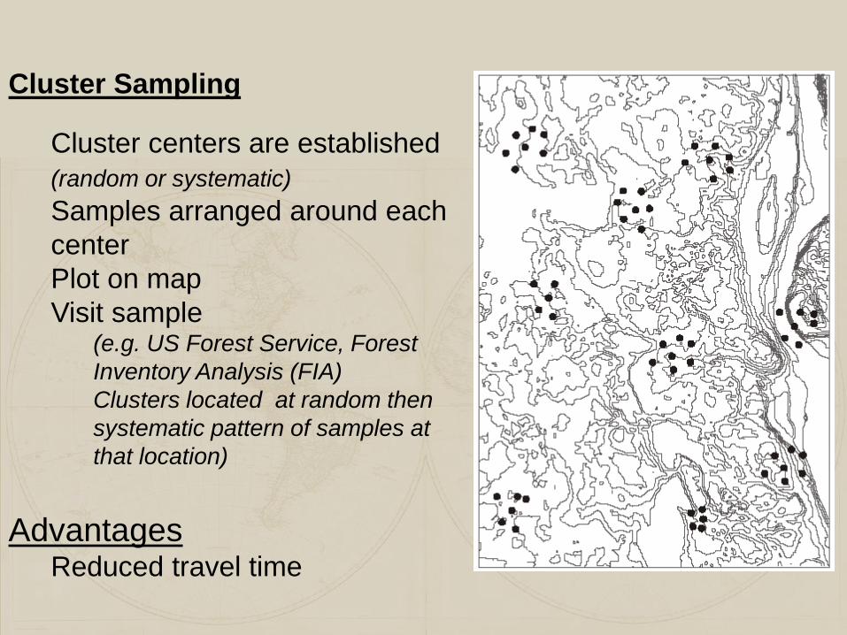
Cluster Sampling
Cluster centers are established
(random or systematic)
Samples arranged around each
center
Plot on map
Visit sample(e.g. US Forest Service, Forest
Inventory Analysis (FIA)
Clusters located at random then
systematic pattern of samples at
that location)
AdvantagesReduced travel time
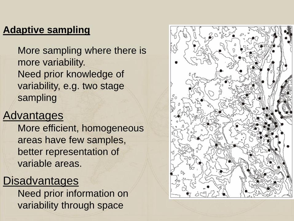
Adaptive sampling
More sampling where there is
more variability.
Need prior knowledge of
variability, e.g. two stage
sampling
AdvantagesMore efficient, homogeneous
areas have few samples,
better representation of
variable areas.
DisadvantagesNeed prior information on
variability through space

INTERPOLATION
Many methods - All combine information about the sample
coordinates with the magnitude of the measurement variable
to estimate the variable of interest at the unmeasured
location
Methods differ in weighting and number of observations
used
Different methods produce different results
No single method has been shown to be more accurate in
every application
Accuracy is judged by withheld sample points
INTERPOLATIONOutputs typically:
Raster surface
•Values are measured at a set of sample points
•Raster layer boundaries and cell dimensions established
•Interpolation method estimate the value for the center of
each unmeasured grid cell
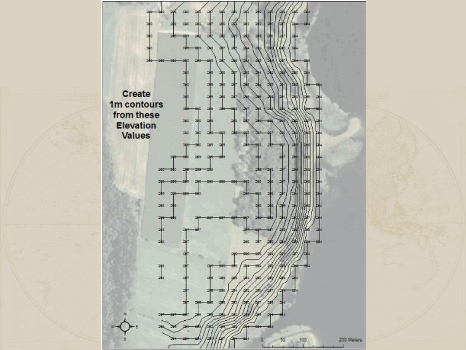
Contour Lines
Iterative process
•From the sample points estimate points of a value Connect
these points to form a line
•Estimate the next value, creating another line with the
restriction that lines of different values do not cross.
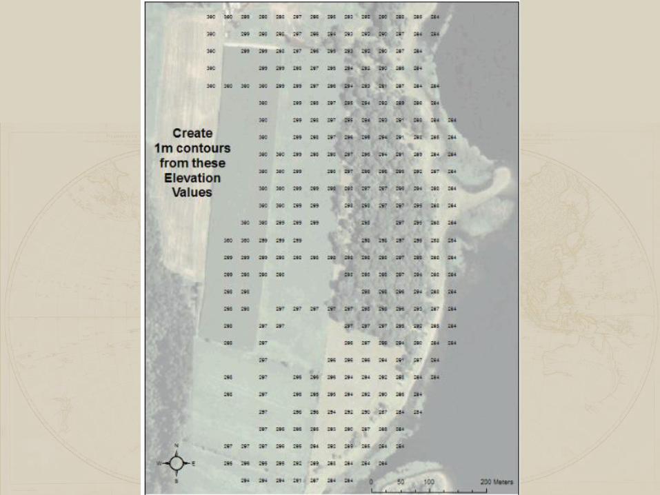

Example Base
Elevation contours Sampled locations and values

INTERPOLATION1st Method - Thiessen Polygon
Assigns interpolated value equal to the value found
at the nearest sample location
Conceptually simplest method
Only one point used (nearest)
Often called nearest sample or nearest neighbor
INTERPOLATION
Thiessen Polygon
Advantage:
Ease of application
Accuracy depends largely on sampling density
Boundaries often odd shaped as transitions between
polygons
are often abrupt
Continuous variables often not well represented

Source: http://www.geog.ubc.ca/courses/klink/g472/class97/eichel/theis.html
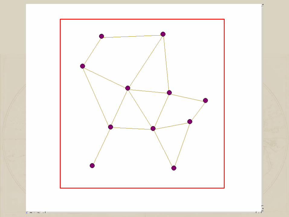
Draw lines
connecting the
points to their
nearest
neighbors.
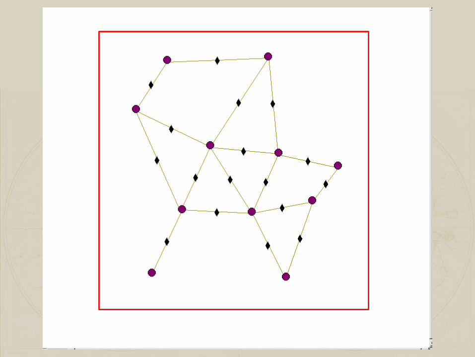
Find the bisectors of
each line.
Connect the
bisectors of the
lines and assign
the resulting
polygon the value
of the center
point
Thiessen Polygon
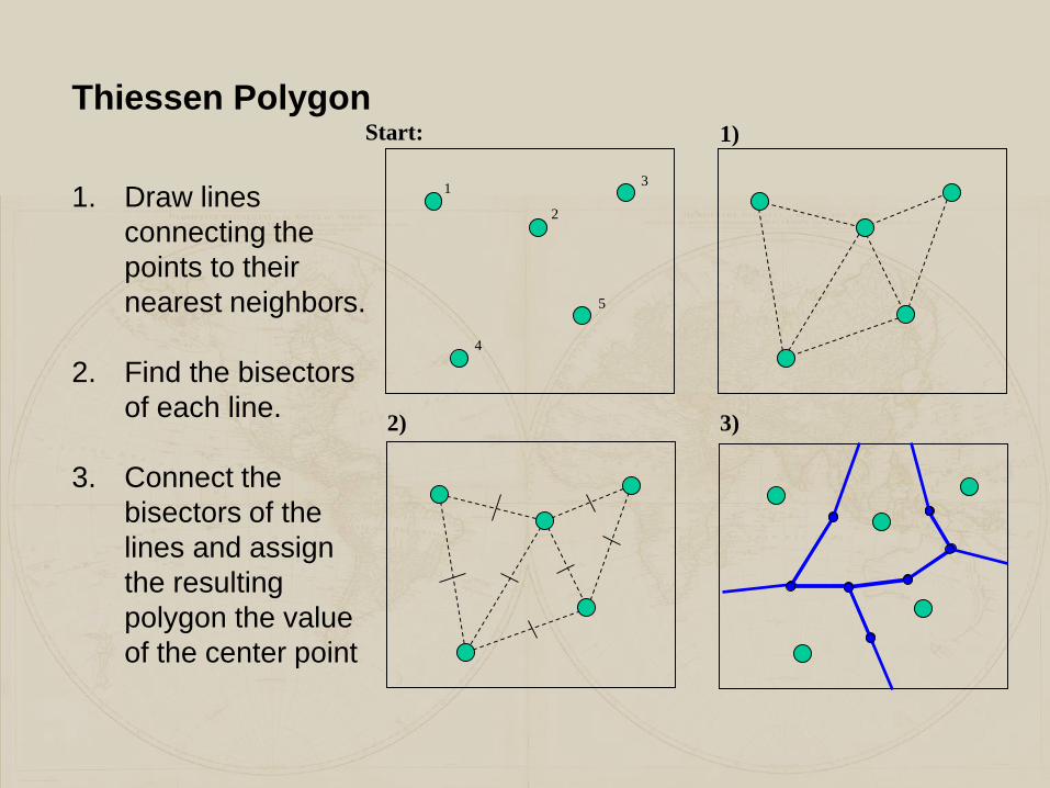
1. Draw lines
connecting the
points to their
nearest neighbors.
2. Find the bisectors
of each line.
3. Connect the
bisectors of the
lines and assign
the resulting
polygon the value
of the center point
Thiessen Polygon
1
2
3
5
4
Start: 1)
2) 3)
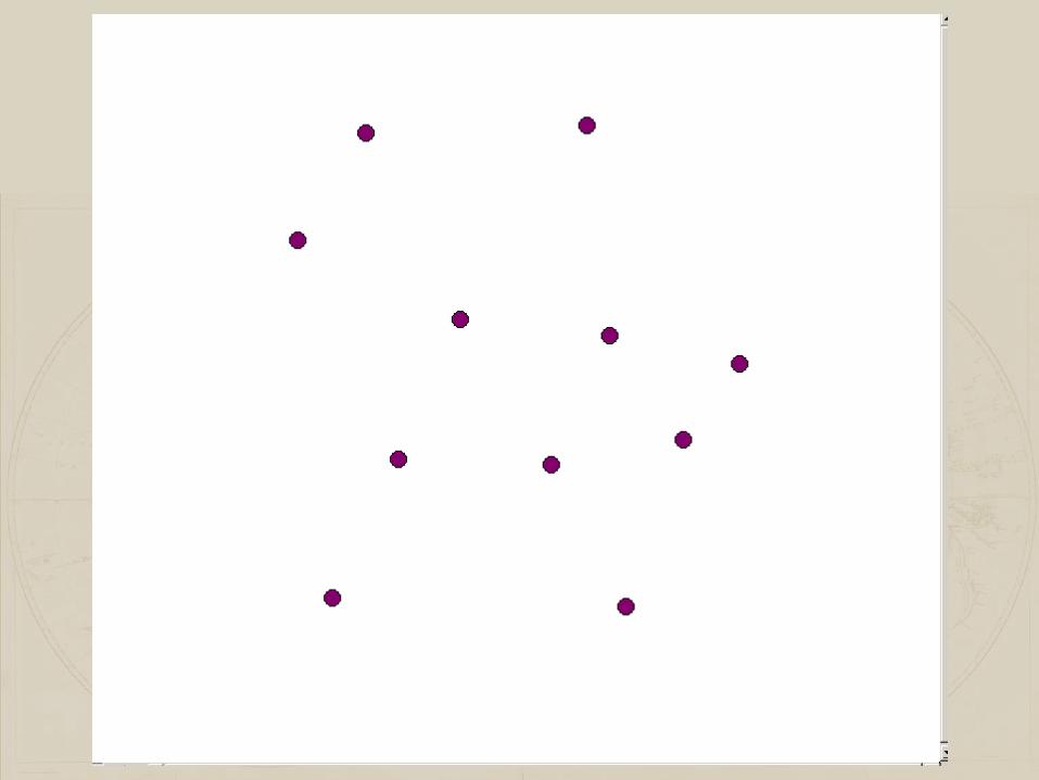

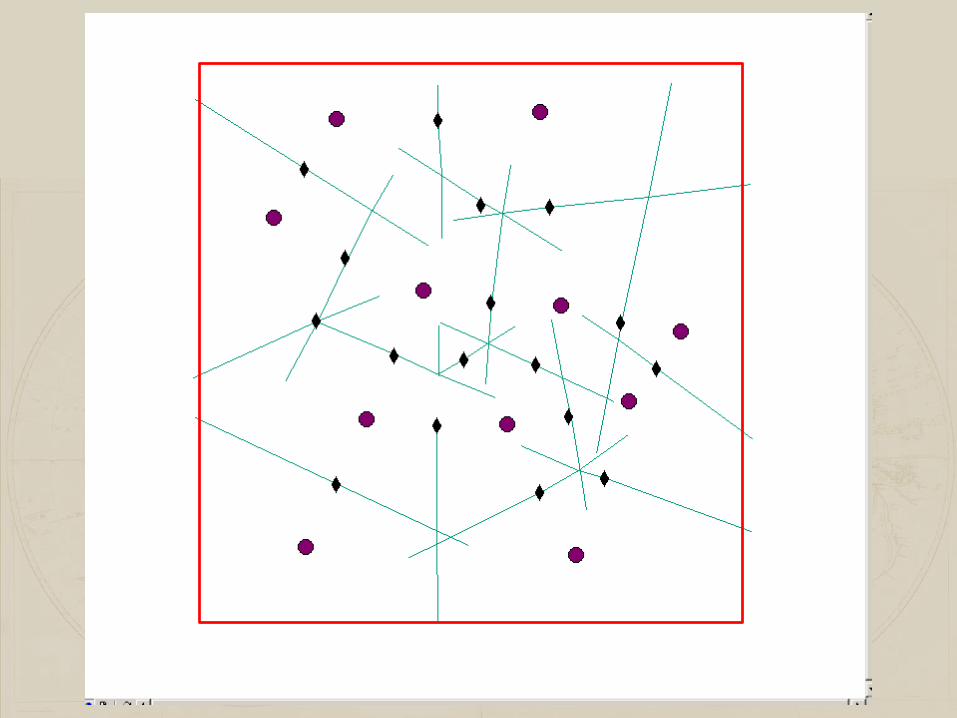

Sampled locations and values Thiessen polygons

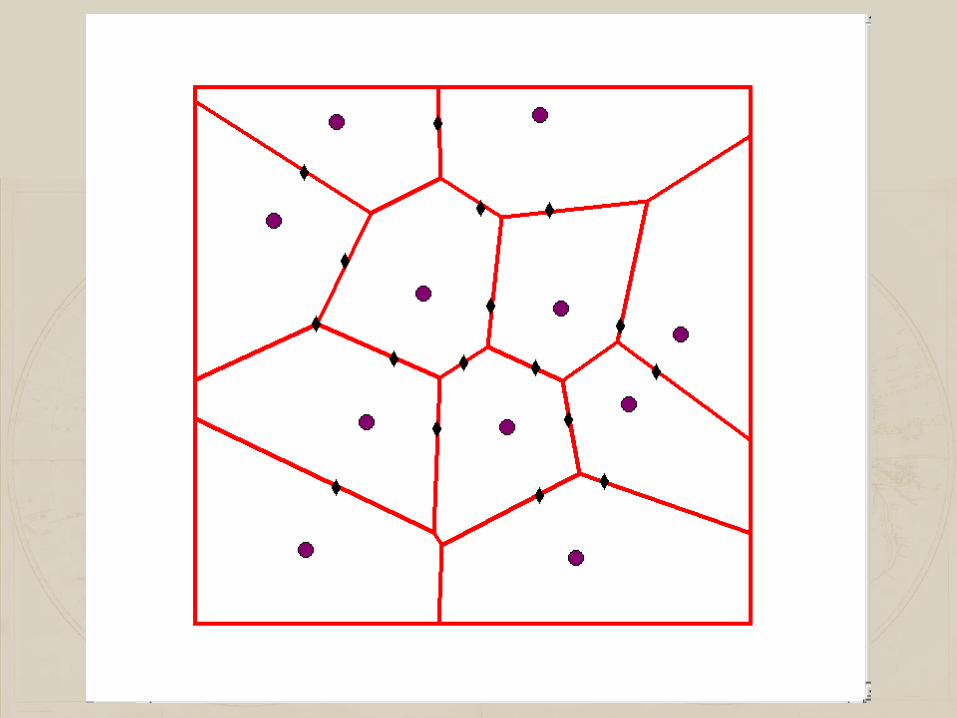
INTERPOLATION Fixed-Radius – Local Averaging
More complex than nearest sample
Cell values estimated based on the average of nearby
samples
Samples used depend on search radius(any sample found inside the circle is used in average, outside ignored)
•Specify output raster grid
•Fixed-radius circle is centered over a raster cell
Circle radius typically equals several raster cell widths(causes neighboring cell values to be similar)
Several sample points used
Some circles many contain no points
Search radius important; too large may smooth the data too
much

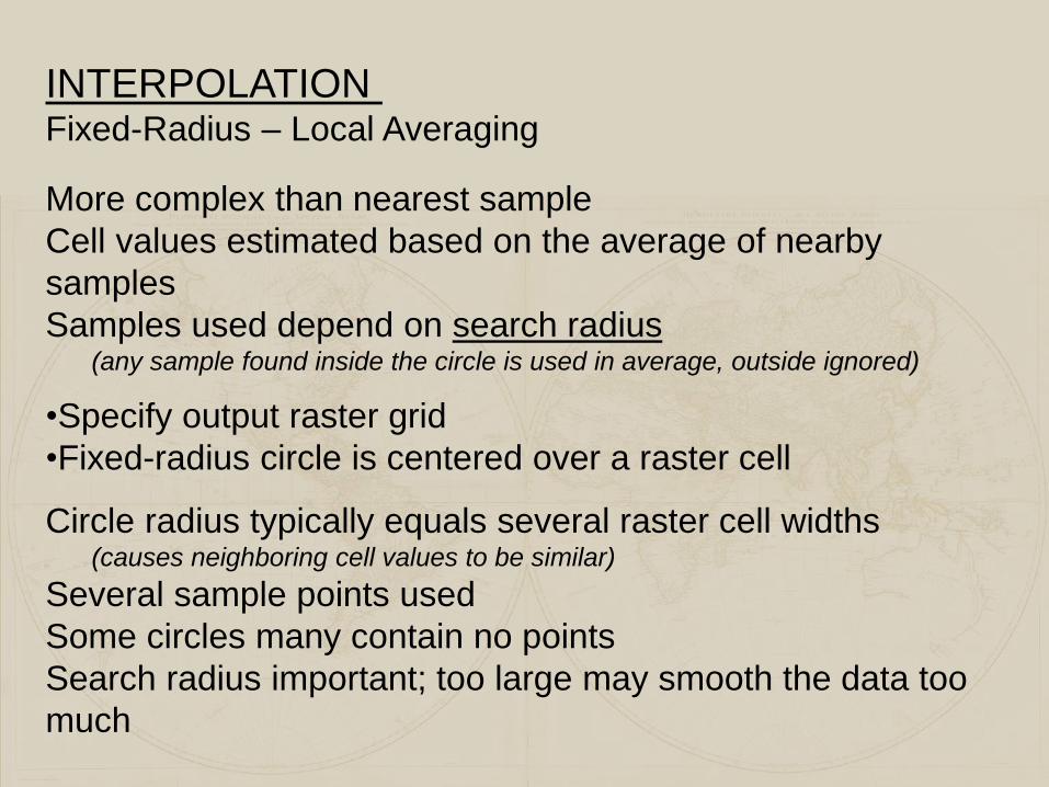
INTERPOLATION
Fixed-Radius – Local Averaging

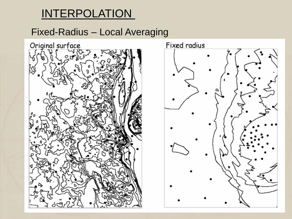
INTERPOLATION
Fixed-Radius – Local Averaging
INTERPOLATION
Fixed-Radius – Local Averaging
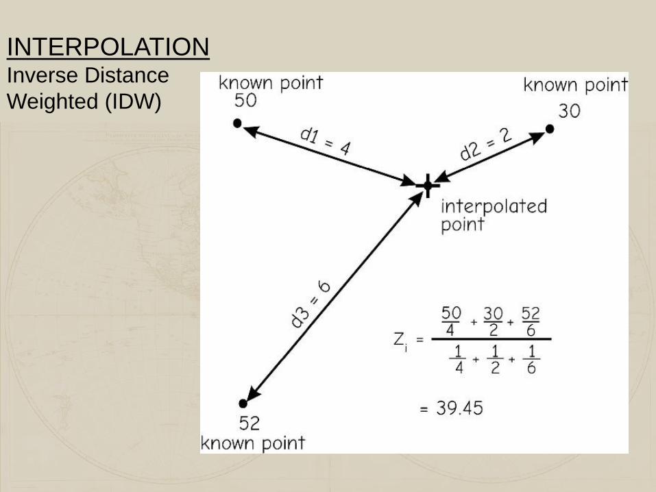
INTERPOLATIONInverse Distance Weighted (IDW)
Estimates the values at unknown points using the
distance and values to nearby know points (IDW reduces
the contribution of a known point to the interpolated value)
Weight of each sample point is an inverse proportion to
the distance.
The further away the point, the less the weight in
helping define the unsampled location

INTERPOLATIONInverse Distance Weighted (IDW)
Zi is value of known point
Dij is distance to known
point
Zj is the unknown point
n is a user selected
exponent
INTERPOLATIONInverse Distance
Weighted (IDW)
INTERPOLATIONInverse Distance Weighted (IDW)
Factors affecting interpolated surface:
•Size of exponent, n affects the shape of the surface
larger n means the closer points are more influential
•A larger number of sample points results in a smoother
surface
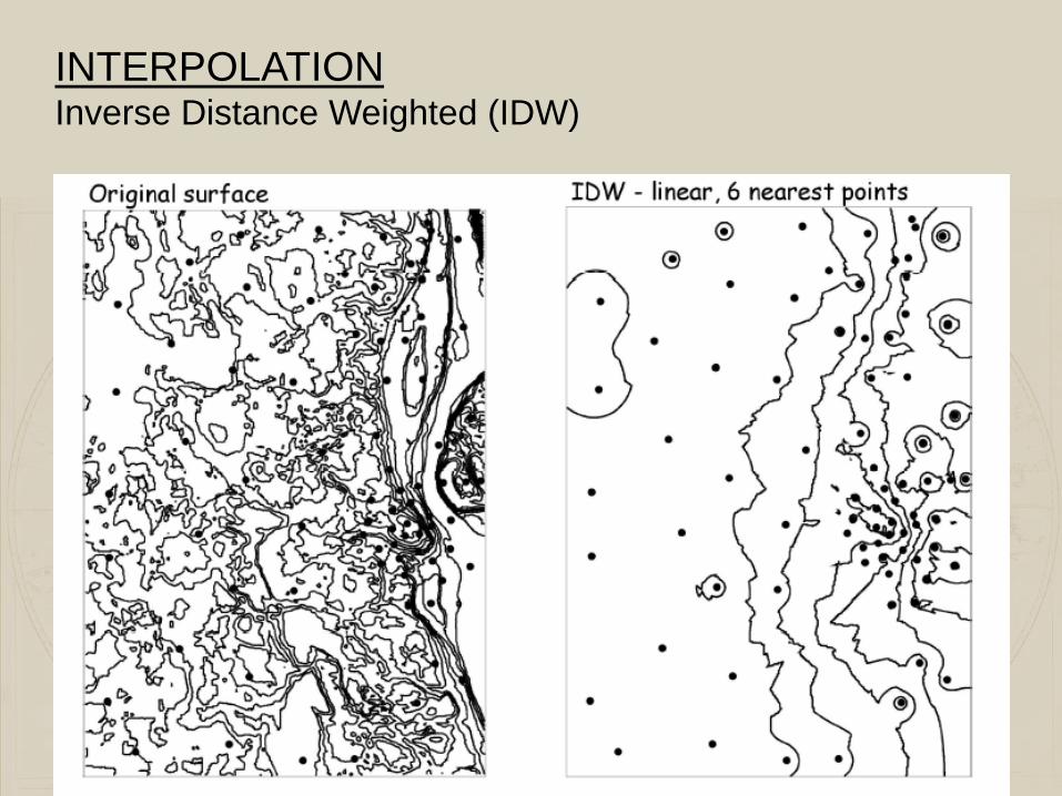
INTERPOLATIONInverse Distance Weighted (IDW)
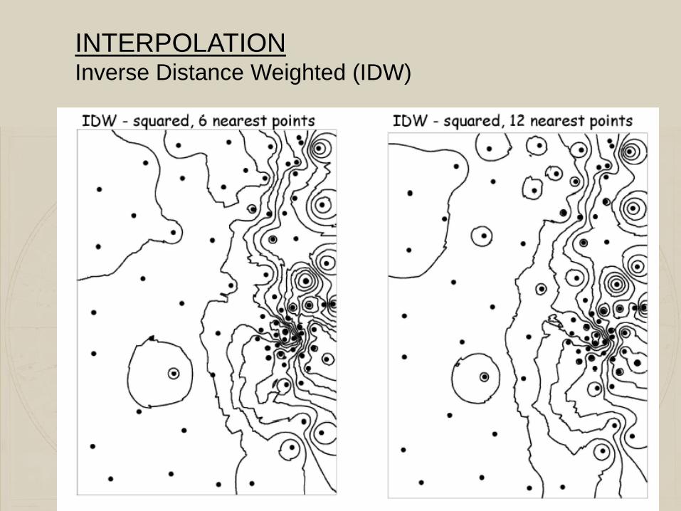
INTERPOLATIONInverse Distance Weighted (IDW)
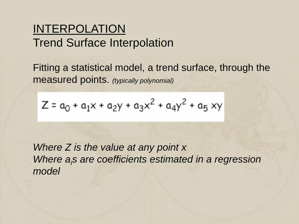
INTERPOLATION
Trend Surface Interpolation
Fitting a statistical model, a trend surface, through the
measured points. (typically polynomial)
Where Z is the value at any point x
Where ais are coefficients estimated in a regression
model

INTERPOLATION
Trend Surface Interpolation

INTERPOLATION
Splines
Name derived from the drafting tool, a flexible ruler, that
helps create smooth curves through several points
Spline functions are use to interpolate along a smooth
curve.
Force a smooth line to pass through a desired set of
points
Constructed from a set of joined polynomial functions

INTERPOLATION : Splines
INTERPOLATION
Kriging
Similar to Inverse Distance Weighting (IDW)
Kriging uses the minimum variance method to
calculate the weights rather than applying an
arbitrary or less precise weighting scheme
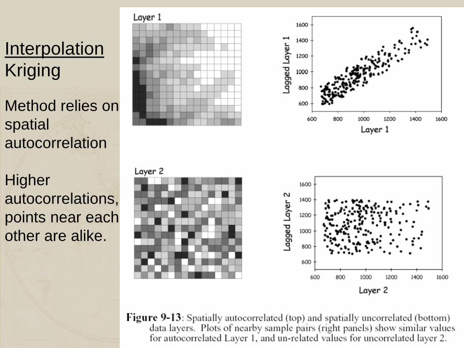
Interpolation
Kriging
Method relies on
spatial
autocorrelation
Higher
autocorrelations,
points near each
other are alike.
INTERPOLATIONKriging
A statistical based estimator of spatial variables
Components:
•Spatial trend
•Autocorrelation
•Random variation
Creates a mathematical model which is used to estimate
values across the surface

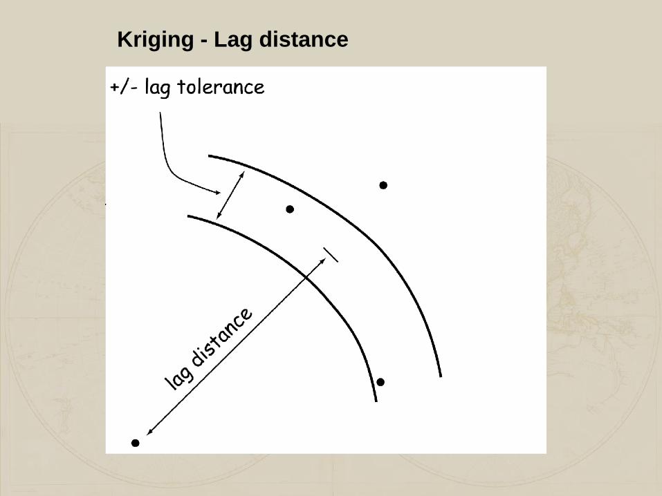
Kriging - Lag distance
Zi is a variable at a sample point
hi is the distance between sample
points
Every set of pairs Zi,Zj defines a
distance hij, and is different by the
amount
Zi – Zj.
The distance hij is the lag distance
between point i and j.
There is a subset of points in a
sample set that are a given lag
distance apart
Kriging - Lag distance

INTERPOLATION Kriging
Semi-variance
Where Zi is the measured variable at one point
Zj is another at h distance away
n is the number of pairs that are approximately h distance
apart
Semi-variance may be calculated for any h
When nearby points are similar (Zi-Zj) is small so the semi-
variance is small.
High spatial autocorrelation means points near each other
have similar Z values

INTERPOLATION
Kriging
When calculating the semi-variance of a
particular h often a tolerance is used
Plot the semi-variance of a range of lag
distances
This is a variogram
INTERPOLATION
Kriging
When calculating the semi-variance of a
particular h often a tolerance is used
Plot the semi-variance of a range of lag
distances
This is a variogram
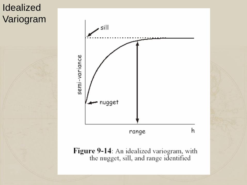
Idealized
Variogram
INTERPOLATION (cont.)
Kriging
•A set of sample points are used to estimate the shape of
the variogram
•Variogram model is made
(A line is fit through the set of semi-variance points)
•The Variogram model is then used to interpolate the entire
surface

Variogram


INTERPOLATION (cont.)
Exact/Non Exact methods
Exact – predicted values equal observed
Theissen
IDW
Spline
Non Exact-predicted values might not equal observed
Fixed-Radius
Trend surface
Kriging
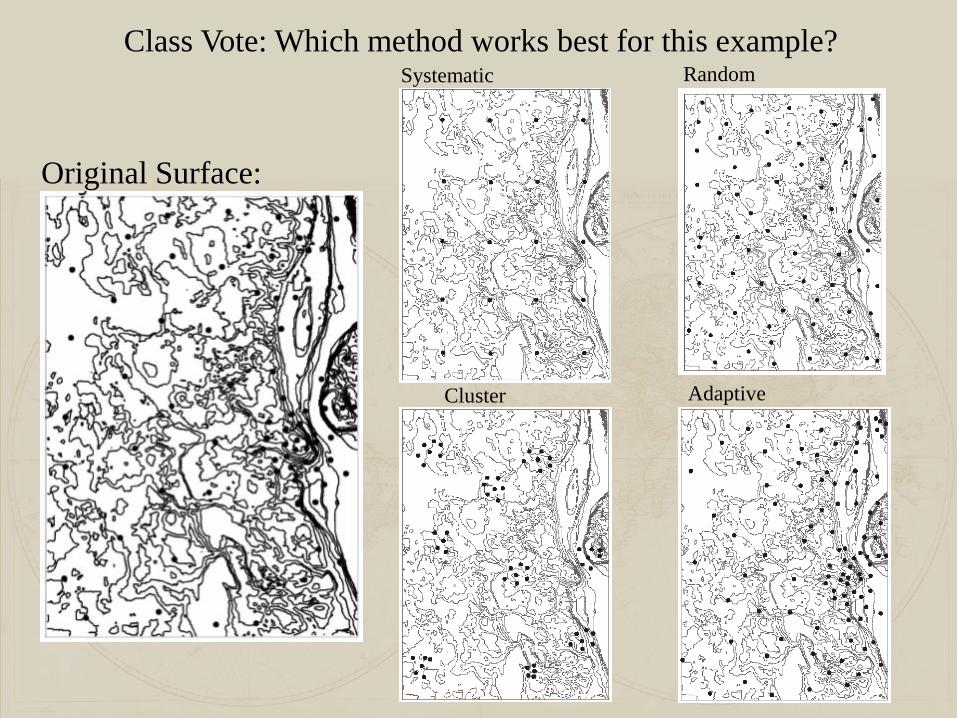
Class Vote: Which method works best for this example?
Original Surface:
Cluster Adaptive
RandomSystematic

Class Vote: Which method works best for this example?
Original Surface:
Thiessen
Polygons
Fixed-radius –
Local Averaging
IDW: squared,
12 nearest points
Trend Surface Spline Kriging
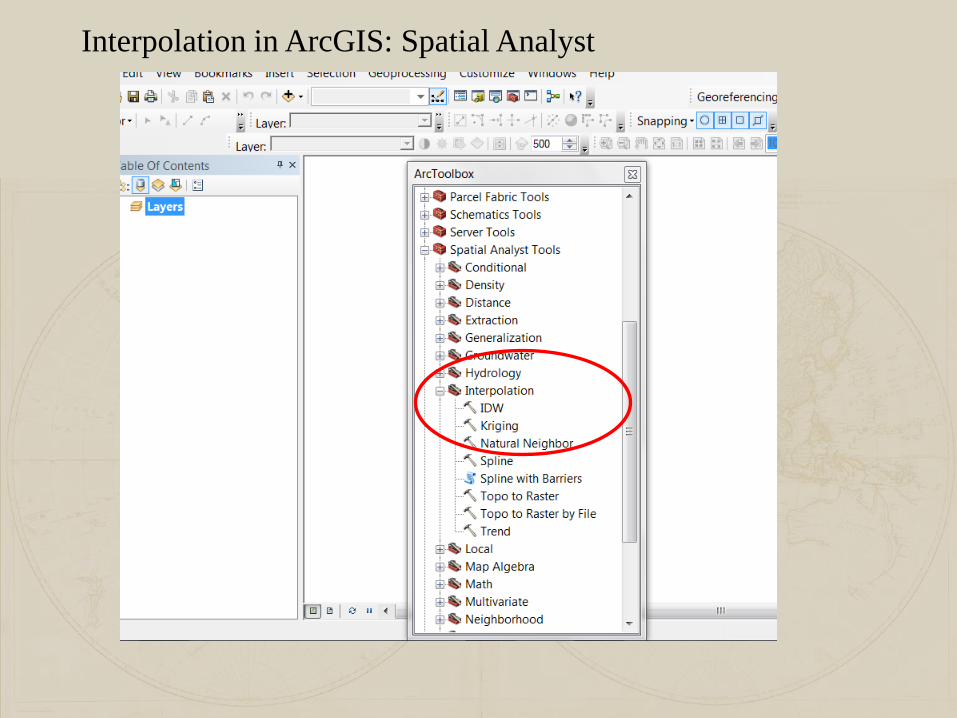
Interpolation in ArcGIS: Spatial Analyst
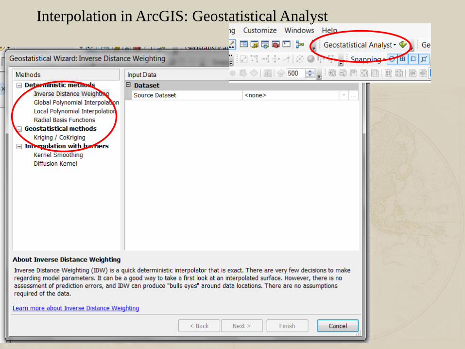
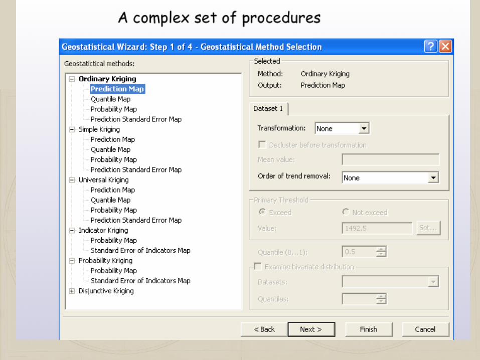
Interpolation in ArcGIS: Geostatistical Analyst

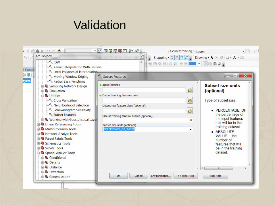
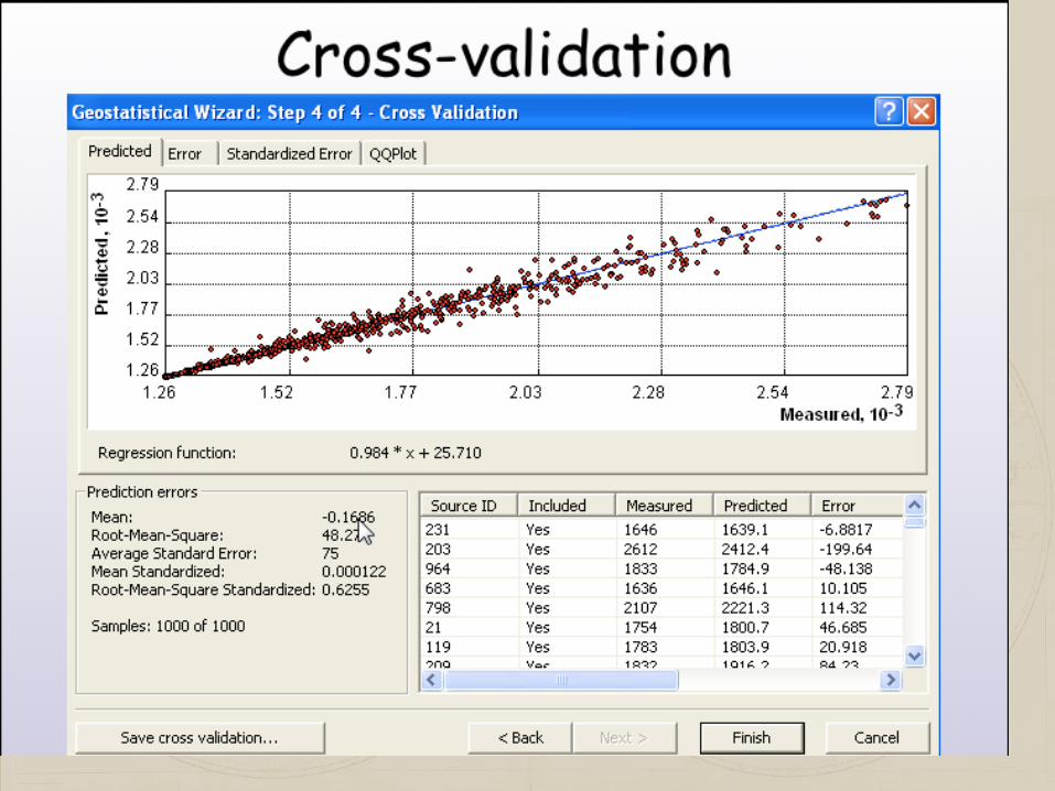
Validation

Interpolation in ArcGIS: arcscripts.esri.com
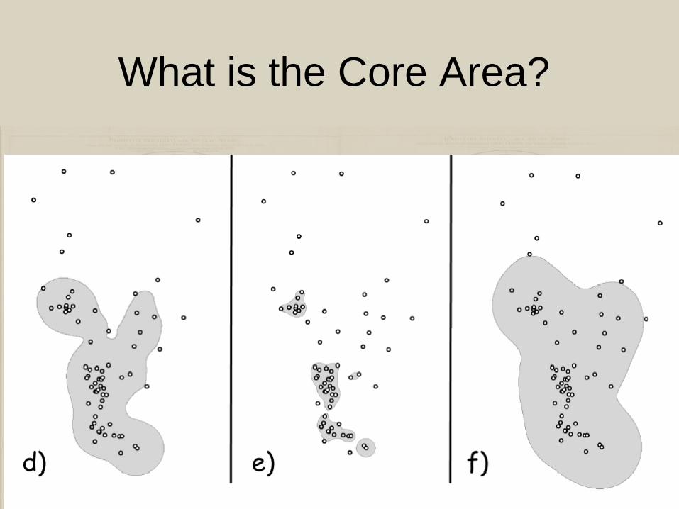
What is the Core Area?
Core Area Identification
• Commonly used when we have
observations on a set of objects, want to
identify regions of high density
• Crime, wildlife, pollutant detection
• Derive regions (territories) or density
fields (rasters) from set of sampling
points.

Mean Circle
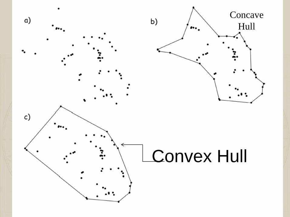
Convex Hull
Concave
Hull


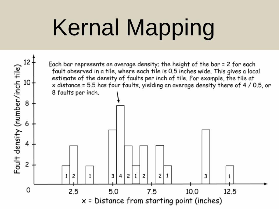
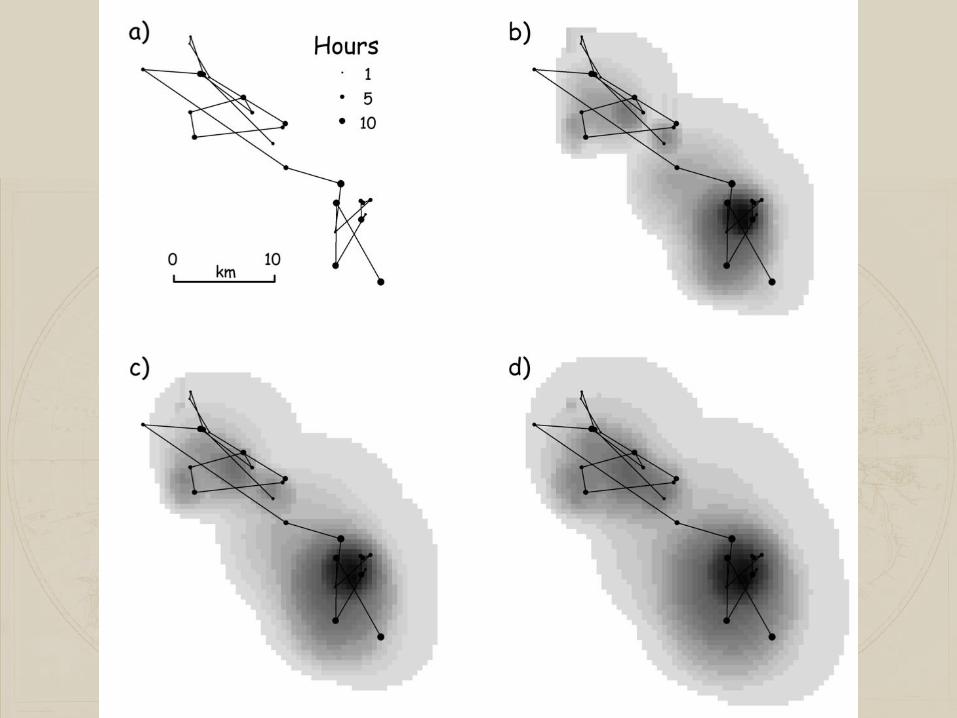
Kernal Mapping

Smooth “density function”
One centered
on each
observation
point

Sum these density functions

Sum the total, for a smooth
density curve (or surface)
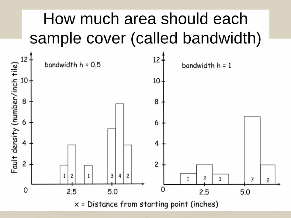
How much area should each
sample cover (called bandwidth)

Varying
bandwidths
a)Medium
b)Low h
c)High h
d through f
are 90%
density
regions

Time-Geographic Density Estimation (TDGE)