interpreting the kohonen self-organizing feature map using contiguity-constrained clustering

ELSEVIER

April 1995

Pattern Recognition Letters 16 (1995) 399-408

Pattern R.ecognition Letters

Interpreting the Kohonen self-organizing feature map using contiguity-constrained clustering

F. Murtagh *

Space Telescope - European Coordinating Facility, European Southern Observatory, Karl-Schwarzschild-Str. 2, D-85748 Garching, Germany

Received 26 June 1994; revised 18 November 1994

Abstract

An interpretation phase is proposed, to complement usage of the Kohonen self-organizing feature map (SOFM) method. This segments the SOFM output, using an agglomerative contiguity-constrained clustering method. We discuss why such a clustering method, which respects contiguity information, should be used. The contiguity-constrained clustering method implemented uses array operations as far as possible, and is thus quite efficient. An application to an astronomical catalog of about a quarter million objects is presented.

Keywords: Cluster analysis; Neural networks; Hierarchical clustering; Regionalization; Segmentation; Data analysis; Image processing

1. The Kohonen SOFM method

The Kohonen self-organizing feature map (SOFM) method may be described in these terms (Kohonen, 1988, 1990; Kohonen et al., 1992; Murtagh and Hernhndez-Pajares, 1994):

1. Each item in a multidimensional input data set is assigned to a cluster center.

2. The cluster centers are themselves ordered by their proximities.

3. The cluster centers are arranged in some spe- cific output representational structure, often a regu- larly spaced grid.

These statements constitute a particular view of the SOFM method. The cluster centers may be re-

* Affiliated to Astrophysics Division, Space Science Depart- ment, European Space Agency. Email: [email protected]

ferred to as "neurons" but a purely algorithmic perspective is adopted here, with no appeal to how the brain stores information in a topological or other manner.

From the viewpoint of the data analyst the SOFM method provides an analysis which is reminiscent of what hierarchical clustering provides: i.e., a number of clusters are obtained, which are additionally structured in some way to facilitate interpretation. Hierar- chical duster analysis is not the only family of data analysis methods which "structure" the output in some way. In fact, one could claim that the need for such "structuring" results from the fact that the old question of what constitutes the inherent number of clusters in a data set can not be answered in any definitive way.

The output representational grid of cluster centers, wi (initially randomly valued), is structured through the imposing of neighborhood relations:

0167-8655/95/$09.50 © 1995 Elsevier Science B.V. All rights reserved SSDI 0167-8655(94)001 13-8

400 17. Murtagh /Pattern Recognition Letters 16 (1995) 399-408

Step O. Consider an input vector ~' from the set of inputs.

Step 1. Determine the cluster center c = i such that II ~ ' - ~')11 is minimum over all i.

Step 2. For all clusters centers i:

w~t+I)~--W~t)'~-oI(t)(x--w~t)) if i~Nc(t) ,

= ~ t ) if i ~ Nc(t)

where O~ (t) is a small fraction, used for controlling convergence; and N~(t) is the neighborhood of duster center c.

Step 3. Increment t; return to Step 0, unless a stopping condition is reached.

An iteration in this algorithm is the assignment, or re-assignment, of an input vector to a cluster center. An epoch is the assignment/re-assignment of all inputs.

The stopping criterion is akin to the stopping criterion used in iterative partitioning methods, e.g. no change in assignment of the input vectors during an epoch. We have found that often 5 or 6 epochs suffice to attain convergence (Murtagh and Hern~mdez-Pajares, 1994). Machine cycles are nowa- days often cheap, though, and rather than expend effort (computational and programming-time) in test- ing for convergence, the implementation used below halted after 10 epochs. As in iterative partitioning methods, there is no guarantee of convergence to a useful solution (a solution which is not "useful" could be, for example, all input vectors assigned to a single class).

Neighborhood in Step 2 defines attraction (inhibi- tion could also be taken into account). The neighborhood can be defined as a "Mexican hat" (difference of Gaussians) on the representational grid of cluster centers. We used a simpler square approximation, and found results to be acceptable. The neighborhood is made to decrease with iterations, towards the best "winner" (as defined by Step 1) duster center. The initial cluster centers are randomly valued, and clearly must be of the same dimensionality as the input data vectors. Different variants on the algorithm steps described above are possible. A description of our exact coded implementation may be found in (Murtagh and Hern~ndez-Pajares, 1994).

The topological relation induced on the cluster

centers is an interesting one. Consider two cluster centers Wl and we which are in the same neighborhood (N c, used in Step 2 above). An input vector is denoted by ~'. Then the triangle with vertices ~1, ~2 and ~' is shape-invariant under the updating carded out by the above algorithm (Murtagh and Hem~indez-Pajares, 1994). More informally ex- pressed we have that: Wl and w2 become more alike, to the extent that they are similar to ~'; and similarity between duster centers is--by definition of the neighborhood--encouraged if they are close on the representational grid.

The output representation has been discussed in terms of clustering. The arrangement of cluster centers, however, leads to a close relationship with a range of widely used dimensionality-reduction methods. Included among these are Sammon nonlinear multidimensional scaling and principal components analysis. For a large input data set (which is the case examined in this article), the output arrangement of cluster centers on a regular grid is close to what is produced by some nonlinear dimensionality-reduction method. The given dimensionality m (that of the vector ~' or ~ above, for example) is mapped into a discretized 2-dimensional space.

2. SOFM and complementary methods

The following two practical problems arise with this SOFM method. Firstly, if a two- or three-duster solution is potentially of interest, it is difficult to specify an output representational grid with just this number of cluster centers. One would be more ad- vised to use a traditional k-means partitioning method. Alternatively, the thought comes to mind to further process the cluster centers, perhaps in a way which is motivated by hierarchical cluster analysis.

The second practical problem is a "bottom-up" version of this same issue. Having a large number of cluster centers poses the problem of summarizing them in some way. Ultsch (1993a, b) has tackled this problem in a graphical way. His approach is to consider II ~'-~'11 where ~ and f are two adjacent duster centers. The regular output representational grid is thus mapped onto a gradient map. A gradient map, defined on a regular grid, suggests the follow-

F. Murtagh /Pattern Recognition Letters 16 (1995) 399-408 401

ing. We can go beyond simple visualization, and carry out a segmentation of the gradient image, and thus the SOFM cluster centers (see (Narendra and Goldberg, 1980) for image data; (Hartigan, 1975; Kittler, 1976, 1979; Shaffer et al., 1979) for point pattern data). This we will do, using contiguity-constrained clustering. We seek to use segmentation, using contiguity-constrained clustering, in order to automate the interpretation approach described by Ultsch.

We could arrive at a segmentation through following image gradients. This can lack robustness (this is the old problem of single linkage and closely associated agglomerative criteria: segments can be undesir- ably formed through indirect relationshipsI"friends of friends"). It also lacks the unified framework resulting from the centroid-based cluster center up- date rules used in the SOFM method. For these two reasons, we will now discuss segmentation methods which form clusters by agglomerating, and which are centroid-based. The corresponding agglomerative criteria are the minimum distance criterion or the minimum variance criterion.

3. Contiguity-constrained clustering

We have seen how cluster centers are formed by the SOFM method in such a way that similarly valued cluster centers are closely located on the representational grid. This reinforces the need for any subsequent clustering of these cluster centers to take such contiguity information into account.

Reviews of contiguity-constrained clustering may be found in (Murtagh, 1985a; Gordon, 1981; Murtagh, 1994). Split-and-merge techniques may well be warranted for segmenting large images. We however seek to segment a grid, at each element of which we have a multidimensional vector, which is ordinarily not of very large dimensions (say, if square, 50 × 50 or 100 × 100). On computational grounds, a pure agglomerative strategy is eminently feasible.

Agglomerative hierarchical clustering algorithms proceed as follows, where the term "cluster" may also refer to a singleton.

Step 1. Find the two closest clusters, 2' and ~'. Agglomerate them, replacing with a cluster center, (see further below).

Step 2. Repeat Step 1, until one cluster only remains.

A common definition of a cluster center is

1 [wl • ~' (1)

qEw

i.e., the mean vector. The term I z [ is the cardinality of the set associated with vector ~. The term "closest" in Step 1 may be defined using the Eu- clidean squared distance as

II 2.- Y'II 2 (2)

o r a s

I x l ' l y l II 2"- •11 z. (3)

I x l + l y l

In expression (2) we have a centroid, minimal distance criterion; and in expression (3) a minimal variance criterion (Murtagh, 1985b).

The contiguity-constrained enhancement on the above algorithm is that in Step 1, we only allow 2' and ~" to be agglomerated if in addition we have: there is some q ~ x and some q' ~ y such that q and q' are contiguous. The definition of contiguity on the regular grid is immediate if we require, for example, that the 8 possible neighbors of a given grid intersec- tion form contiguous neighbors. Note that this definition of contiguity is quite a weak one, and note that there will always be contiguous clusters (unless only one cluster remains).

The problem of inversions or reversals in the series of agglomerations is likely to arise with this general contiguity-constrained algorithm. The reversals problem is as follows. We would like the closest clusters to merge first, followed by progressively looser groupings. That is, if 2' and ~' merge, then the dissimilarity leading to this merging should (we would wish) be less than the dissimilarity between the new cluster and some ~':

d(xUy, z) > d(x, y).

If this is the case, stopping the series of agglomerations at any point ensures an unambiguous partition. However, the centroid criterion, even when uncon- strained, is not guaranteed to adhere to this no-inversions requirement. In the contiguity-constrained case,

402 F. Murtagh / Pattern Recognition Letters 16 (1995) 399-408

it can be shown that only one criterion guarantees a no-reversals sequence of agglomerations. This is the criterion related to complete-linkage clustering:

d(x , y) = m a x { d ( q , q ' ) l q ~ x , q' ~y} .

In spite of reversals in the agglomerative criterion, we will stay with the centroid and variance methods described above. This is because an advan- tage of such methods is that we have a definition of duster center following each agglomeration. There is no similar, unambiguous definition in the case of the complete-linkage criterion. Beaulieu and Goldberg (1989) discuss the minimum variance contiguity- constrained criterion (mistakenly stating that reversals are excluded).

Computational savings can result from carrying out agglomerations, as far as allowed by the data, in parallel. Tilton (1988, 1990) describes such an algorithm. A framework for "cleanly" carrying out agglomerations takes local information only into account. A range of highly efficient algorithms which carry out agglomerations locally have been devel- oped under the names of "reciprocal nearest neighbor" and "nearest neighbor chain" algorithms (Murtagh, 1985b). These use locally based agglomerations to arrive at identical results as achieved by global minimization, in order to define a new agglomeration at each iteration. It is shown in (Murtagh, 1994) that the complete-linkage contiguity-constrained method allows these locally based imple- mentations to be used, without loosing the no-reversals property. Given our preference for methods based on a cluster center, we draw the following conclusion: the possible occurrence of reversals means that we must be additionally vigilant when employing locally based agglomerations, in order not to further exacerbate the interpretation-related difficulties resulting from reversals.

4. CCC implementation

The algorithm used is as follows. To concretize our description, consider an SOFM output which consists of a regular square grid of dimensions 50 × 50. Each cluster center, associated with a grid inter- section, is m-valued if the input vectors are m-valued. We input this 50 X 50 × m array as m separate 50 x 50 arrays.

We make use of a cluster label array of dimensions 50 X 50, initialized to 1, 2 . . . . . 2500.

Let the operation SHIFT, defined on array A, be defined as the moving of each pixel one step in a given direction, with wraparound: A - o SHIFT[A, north]. The squared distances between each pixel of A, with each pixel to its south, is then quite simply ( A - SHIFT[A, north]) 2, where the exponentiation is an array operation. When we are dealing with multivalued pixels, as here, what we have just described is an additive component of the desired array of distances.

Having the distances, we then obtain the global minimum value at each iteration (taking care not to allow zero self-distance). The calculation of Eu- clidean squared distances using array operations is ordinarily computationally efficient.

The following routine was implemented in the IDL (IDL, 1992) image processing programming language.

Step 1. For each pixel, determine its distances with each of the 8 adjacent pixels. Determine the global minimum distance.

Step 2. Let x and y be the cluster labels associated with the pixels associated with the minimum distance. Replace all occurrences of y in the cluster indicator array with x. In each of the m arrays defining the data replace all values associated with label x with their mean value.

Step 3. Repeat until only one cluster, or a user-defined number of dusters, remain.

The algorithm can be updated for a minimum variance homogeneity by taking account of the number of pixels associated with a cluster; and by using the dissimilarity formula given in expression (3).

In the framework of the minimum variance criterion, we can additionally take into account the numbers of input objects associated with each bin of the 50 x 50 SOFM map. This is possible using expression (3). In the application described in the next section, we found that taking all SOFM-produced information into account in this manner (a) led to a greater number of reversals in the sequence of agglomerations, and (b) departed from the mathemati- cal/geometrical framework used in the SOFM method. For these reasons, we employed the centroid agglomerative method in the application described n o w .

F. Murtagh / Pattern Recognition Letters 16 (1995) 399-408 403

5. Application

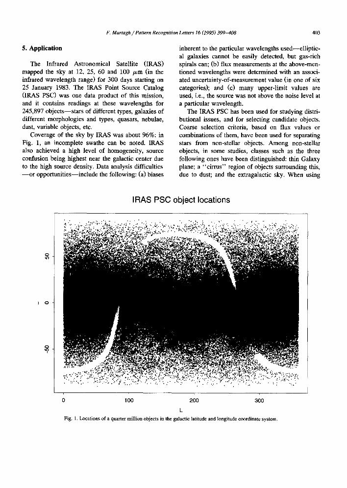
The Infrared Astronomical Satellite (IRAS) mapped the sky at 12, 25, 60 and 100 /xm (in the infrared wavelength range) for 300 days starting on 25 January 1983. The IRAS Point Source Catalog (IRAS PSC) was one data product of this mission, and it contains readings at these wavelengths for 245,897 objects--stars of different types, galaxies of different morphologies and types, quasars, nebulae, dust, variable objects, etc.

Coverage of the sky by IRAS was about 96%: in Fig. 1, an incomplete swathe can be noted. IRAS also achieved a high level of homogeneity, source confusion being highest near the galactic center due to the high source density. Data analysis difficulties - -o r opportunities--include the following: (a) biases

inherent to the particular wavelengths used--elliptic- al galaxies cannot be easily detected, but gas-rich spirals can; (b) flux measurements at the above-men- tioned wavelengths were determined with an associated uncertainty-of-measurement value (in one of six categories); and (c) many upper-limit values are used, i.e., the source was not above the noise level at a particular wavelength.

The IRAS PSC has been used for studying distri- butional issues, and for selecting candidate objects. Coarse selection criteria, based on flux values or combinations of them, have been used for separating stars from non-stellar objects. Among non-stellar objects, in some studies, classes such as the three following ones have been distinguished: thin Galaxy plane; a "cirrus" region of objects surrounding this, due to dust; and the extragalactic sky. When using

IRAS PSC object locations

Q tO

O

O

0 I O0 200 SO0

L

Fig. 1. Locations of a quarter million objects in the galactic latitude and longitude coordinate system.

404 F. Murtagh ~Pattern Recognition Letters 16 (1995) 399-408

• ..,:.~,~- -~... • ~.... : :~" ,L~ K.., • • ...-

• .+:. ,.:~. ~ g l ~ : . .

. . . • • " . ' , . ~ . , ~ . . : " • . . . . - . . + . ; + ; , , .

• • " • - . • " . " ~ L ' . : ' . • . "

• ".. ~.;~ ..,"+.'i': . .

• . • . , , . ~ . , . ~ , S + • . ; " ~ . ~ ~ ' . :+" - .< ;~ •

.++..'p~ ~:" .,': . ; • . ; . e , . . . . . ; . . W , . . . . + , .

:. ".+,,~. ,¢ b+":- . • . . + . : . I . " -

+ . ~ , i~l ,~+.: .: . ' . . - .

• ; , ~ .'+.,,. .

• • ~ . ~ ; , - i , .

0~; 0 OG-

.:'~ ~ . . , . ~..:,.-.. : :~.,. .

~'~..

: ~ . : . ; . .

:i/.+ :+

O~ 0 0~ "

I :,

i:

3.-

i

.!B

~ ! ~ : > : ~ , _ -- ~ ~, , ~ ~

OG 0 OG-

• - . . .~ .... : . : . : ' . • . " - " : ' . . . .+q.~.,~'..t.. '

.. , . ; . ? . "~:.-:.': . . . . . . . . . . . : ; . : ? . . ~..~ .. ; . .

. . . . . . . :..;, : : , . . . . • . " . . o. "~.'..?...! : ~ . . . . . . .

: , ..,:,+,~:~, .+',, . '

• " ' " ' ~ +~.,~ "..+." V . :. " :

• " . : " ! ~ : . . : ' ~ ? . , . : . . . . • , . ; ' , - , , " ' ~ + ~ + ~ , - , , : , ,

• . . ~ ' - ~ ; • , . ~ - . - . . : : . . •

• . : " - : ' " ' , ' " i : ~ ,~ ; ' - . : . : .. + . . : " b;.", " . " . . ,

4 . . . " " L . ' ~ ; " . - ," " , "

. . --. ' : : ;- ' . . : .~x..~':,. ". .. • . .~)......,. ;, . . . . j , •

• , . , ,, • ~.," , . . :+ , • .

: [ . . : " . ' . : . : .:~ .

( ~ 0 0~ "

• . . : ~ ~ , , , ' . .

: " : 'L .~',' ":;" ,. ~,:..: ~-. :..

<?!ii:" :; ~:o.

• . . i ° , ~ : : . . . .

." ";'?, ':;"t.:: • ~ -. . .

0

w

|

,..: ;:

• :~..~ •

.%.

0

e~

..=

~s

8

0

o

o

. m

|

8

Og 0 Og" 0~; 0 OS" OG 0 OG"


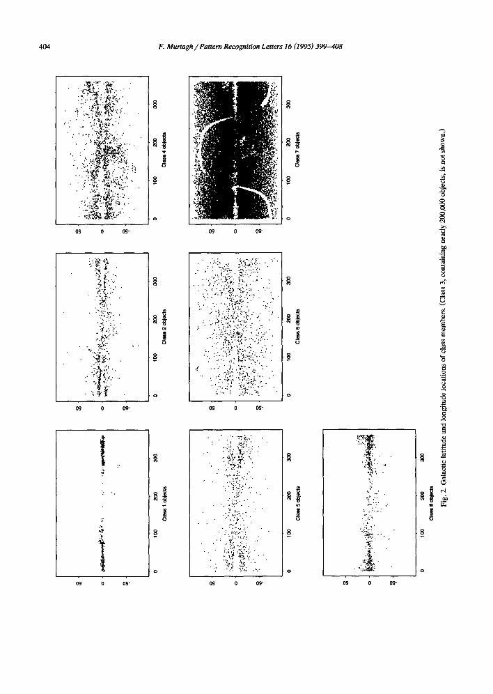
different normalizations of the input data, and different agglomerative criteria, we used this prior information (see Prusti et al., 1992; Boiler et al., 1992; Meurs and Harmon, 1988) to select one result for presentation (in Fig. 2) over others.

No preliminary selections were made: all 245,897 objects were used. These are shown in Fig. 1, in

Table 1 SOFM output: 50 × 50 regular grid

33333333333333333333333111333333333333333333333333 33333333333333333333333111333333333333333333333333 33333333333333333333333333335333333333333333333333 33333333333333333333333333333333333333333333333333 33333333333333333333333333333333333333333333333333 33333333333333333333333333333333333333333333333333 33333333333333333333333333333333333333333333333333 33333333333333333333333333333333333333333333333333 33333333333333333333333333333333333333333333333333 33333333333333333333333333333333333333333333333333 33333333333333333333333333333333333333333333333333 33333333333333333333333333333333333333333333333333 33333333333333333333333333333333333333333333333333 33333333333333333333333333333333333333333333333333 33333333333333333333333333333333333333333333333333 22333333333333333333333333333333333333333333333333 22733333333333333333333333333333333333333333333333 22773333333333333333333333333333333333333333333333 22777733333333333333333333333333333333333333333333 77777733333333333333333333333333333333333333333333 77777733333333333333333333333333333333333333333333 77777733333333333333333333333333333333333333333333 77777333333333333333333333333333333333333333333333 77777333333333333333333333333333333333333333333333 77777333333333333333333333333333333333333333333333 77733333333333333333333333333333333333333333333333 77733333333333333333333333333333333333333333333333 77773333333333333333333333333333333333333333333333 77777333333333333333333333333333333333333333333333 77777733333333333333333333333333333333333333333333 77777777777733333333333333333333333333333333333333 77777777777773333333333333333333333333333333333333 77777777777773333333333333333333333333333333333333 77777777777773333333333333333333333333333333333333 77777777777773333333333333333333333333333333333333 77777777777777333333333333333333333333333333333333 77777777777777333333333333333333333333333333333333 77777777777777733333333333333333333333333333333344 77777777777777733333333333333333333333333333333344 77777777777777777733333333333333333333333333333344 77777777777777777777333333333333333333333333334444 77777777777777777777777733333333333333333333334444 77777777777777777777777733333333333333333333333444 77777777777777777777777777333333333333333333333344 77777777777777777777777777773333333333333333333344 77777777777777777777777777777333333333333333333344 77777777777777777777777777777333333333333333333388 77777777777777777777777777777333333333333333333388 55557777777777666667777777777733333333333333333388 55557777777777666666777777777753333333333333333388

galactic latitude (0 to 360 degrees) and longitude ( - 9 0 to + 90 degrees) coordinates. A set of four variables was derived from the four flux values (F12,F25,F6o, F I 0 0 ) , in line with the studies cited above:

c,2 = Iog( Flz/F25), C23 = Iog( Fzs/F6o),

c34 = log(F6o/Floo), and log F100.

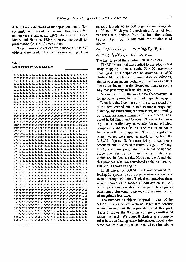
The first three of these define intrinsic colors. The SOFM method was applied to this 245897 × 4

array, mapping it onto a regular 50 × 50 representational grid. This output can be described as 2500 clusters (defined by a minimum distance criterion, similar to k-means methods); with the cluster centers themselves located on the discretized plane in such a way that proximity reflects similarity.

Normalization of the input data (necessitated, if for no other reason, by the fourth input being quite differently valued compared to the first, second and third), was carried out in two manners: range-normalizing, by subtracting the minimum, and dividing by maximum minus minimum (this approach is fa- vored in (Milligan and Cooper, 1988)); or by carrying out a preliminary correlation-based principal components analysis (PCA). The results shown in Fig. 2 used the latter approach. Three principal component values were used as input, for each of the 245,897 objects. Such normalizing is commonly practiced but is viewed negatively e.g. in (Chang, 1983), since mapping into a principal component space may destroy the classificatory relationships which are in fact sought. However, we found that this provided what we considered as the best end-result and is shown in Fig. 2.

In all cases, the SOFM result was obtained following 10 epochs, i.e., all objects were successively cycled through 10 times. Typical computation times were 9 hours on a loaded SPARCstation 10. All other operations described in this paper (contiguity- constrained clustering, display, etc.) required orders of magnitude less time.

The numbers of objects assigned to each of the 50 x 50 cluster centers were not taken into account when carrying out the segmentation of this grid. Table 1 shows the 8-cluster contiguity-constrained clustering result. We chose 8 clusters as a compro- mise between having some information about a desired set of 3 or 4 clusters (cf. discussion above


-0.01

PC2

0.0 0.01 0.02 -0.01

PC2

0.0

6 .6

o

0.01 0.02 i

-0.01

PC2

0.0 0.01 i

0.02

o

9

PC2

-0.01 0.0 0.01 0.02

-0.01

PC2

0.0 0,01

• ( . . , ~ - ? : ; ,

0.02

o

PC2

-0.01 0.0 0,01 0.02

-0,01

PC2

0.0 i

. - . . , . - - . . . . . . , • . .

0.01 0.02

.6 =8

o

o b

PC2

-0.01 0.0 0.01 0.02

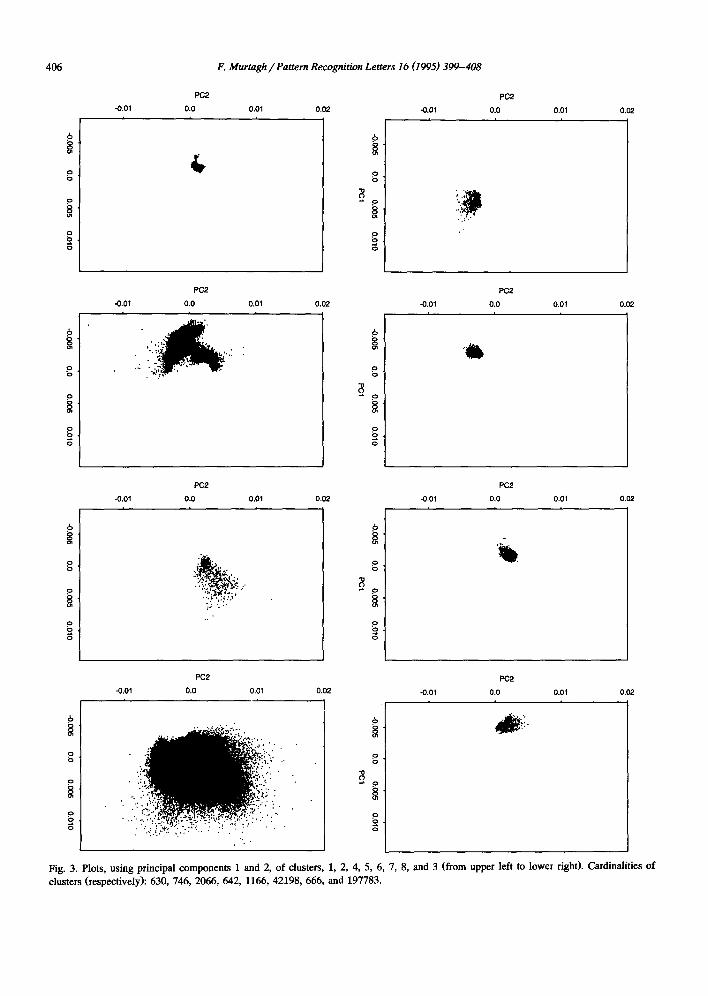
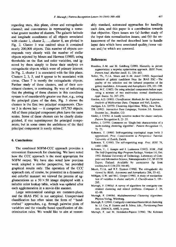
Fig. 3. Plots, using principal components 1 and 2, of clusters, 1, 2, 4, 5, 6, 7, 8, and 3 (from upper left to lower right)• Cardinalities of clusters (respectively): 630, 746, 2066, 642, 1166, 42198, 666, and 197783.


regarding stars, thin plane, cirrus and extragalactic classes); and convenience in representing a some- what greater number of clusters. The galactic latitude and longitude coordinates of all objects associated with cluster 1, cluster 2 . . . . . cluster 8, are plotted in Fig. 2. Cluster 3 was omitted since it contained nearly 200,000 objects. This number of objects cor- responds very closely with the number of stellar objects rejected by Meurs and Harmon (1988), using thresholds on the flux and color variables, and ig- nored by them simply to focus their analysis on extragalactic objects which were of primary interest. In Fig. 2, cluster 1 is associated with the thin plane. Clusters 2, 3, 5, and 8 appear to be associated with cirrus. Class 7 is mostly the extragalactic objects. Further study of these clusters, and of their con- stituent clusters, is continuing. By way of indicating that the plotting of these clusters in this coordinate system is of considerably greater use than, e.g., using the principal plane of the data, Fig. 3 shows the clusters in the first two principal components. Clus- ter 3 is shown last - - it comprises 197,783 objects. All of these principal component plots have the same scales. Some of these clusters can be clearly distinguished, if one superimposes the principal components; but in some cases the usefulness of the third principal component is sorely missed.

6. Conclusions

The combined SOFM-CCC approach provides a convenient framework for clustering. We have noted how the CCC approach is the most appropriate for SOFM output. We have also noted how previous work adopted a similar perspective, but provided graphical results only. The operation of the CCC approach can, of course, be presented in a dynamical and colorful manner: we viewed the process of agglomerations as a 50 × 50 image displayed with a suitable color lookup table, which was updated after each agglomeration in a movie-like manner.

Large astronomical catalogs are common-place, and the IRAS PSC is not untypical. Unsupervised classification has often taken the form of "hand- crafted" approaches, e.g. through pairwise plots of variables and the visually based specification of dis- crimination rules. We would like to aim at reason-

ably standard, automated approaches for handling such data, and this paper is a contribution towards that objective. Open issues are (a) further study of the input data normalization issues; and (b) the enhancement of the method described here to handle input data which have associated quality/error values and/or which are censored.

References

Beaulieu, J.-M. and M. Goldberg (1989). Hierarchy in picture segmentation: a stepwise optimization approach. IEEE Trans. Pattern Anal Machine lntell. 11, 150-163.

Boiler, Th., E.J.A. Meurs and H.-M. Adorf (1992). Supervised selection of galaxy candidates from the IRAS PSC--The quality of the selection and the infrared properties of the galaxy candidates. Astronomy and Astrophysics 259, 101-108.

Chang, W.C. (1983). On using principal components before separating a mixture of two multivariate normal distributions. Appl. Statist. 32, 267-275.

Gordon, A.D. (1981). Classification: Methods for the Exploratory Analysis of Multivariate Data. Chapman and Hall, London.

Hartigan, J.A. (1975). Clustering Algorithms. Wiley, New York. IDL (1992). Interactive Data Language, Version 3.0. Research

Systems Inc., Boulder, CO. Kittler, J. (1976). A locally sensitive method for cluster analysis.

Pattern Recognition 8, 23-33. Kittler, J. (1979). Comments on 'Single-link characteristics of a

mode-seeking clustering algorithm'. Pattern Recognition 11, 71-73.

Kohonen, T. (1988). Self-organizing topological maps (with 5 appendices). Proc. Connectionism in Perspective: Tutorial. University of Zurich, Zurich.

Kohonen, T. (1990). The self-organizing map. Proc. IEEE 78, 1464-1480.

Kohonen, T., J. Kangas and J. Laaksonen (1992), SOM_ PAK The Self-Organizing Map Program Package, Version 1.0, Oct. 1992. Helsinki University of Technology, Laboratory of Com- puter and Information Science, Rakentajanaukio 2 C, SF-02150 Espoo, Finland. Available by anonymous ftp from cochlea.hut.fi (130.233.168.48).

Meurs, E.J.A. and R.T. Harmon (1988). The extragalactic sky viewed by IRAS. Astronomy and Astrophysics 206, 53-62.

Milligan, G,W. and M.C. Cooper (1988). A study of standardiza- tion of variables in cluster analysis. J. Classification 5, 181- 205.

Murtagh, F. (1985a). A survey of algorithms for contiguity-constrained clustering and related problems. Computer J. 28, 82-88.

Murtagh, F. (1985b). Multidimensional Clustering Algorithms. Physica-Verlag, Wiirzburg.

Murtagh, F. (1994). Contiguity-constrained hierarchical clustering. In: I.J. Cox, P. Hansen and B. Julesz, Eds., Partitioning Data Sets. DIMACS, AMS, in press.

Murtagh, F. and M. Hern~ndez-Pajares (1994). The Kohonen


self-organizing map method: an assessment. J. Classification, in press.

Narendra, P.M. and M. Goldberg (1980). Image segmentation with directed trees. IEEE Trans. Pattern Anal. Machine Intell. 2, 185-191.

Prusti, T., H.-M. Adorf and E.J.A. Meurs (1992). Young stellar objects in the IRAS Point Source Catalog. Astronomy and Astrophysics 261, 685-693

Shaffer, E., R. Dubes and A.K. Jain (1979). Single-link characteristics of a mode-seeking clustering algorithm. Pattern Recog- nition 11, 65-70.

Tilton, J.C. (1988). Image segmentation by iterative parallel region growing with application to data compression and image

analysis. Proc. Symposium on the Frontiers of Massively Parallel Computation, NASA, Greenbelt, MD, 357-360.

Tilton, J.C. (1990). Image segmentation by iterative parallel region growing. Information Systems Newsletter, February, 50- 52.

Ultsch, A. (1993a). Knowledge extraction from self-organizing neural networks. In: O. Opitz, B. Lausen and R. Klar, Eds., Information and Classification. Springer, Berlin, 301-306.

Ultsch, A. (!993b). Self-organizing neural networks for visualization and classification. In: O. Opitz, B. Lausen and R. Klar, Eds., Information and Classification. Springer, Berlin, 307- 313.

interpreting the kohonen self-organizing feature map using contiguity-constrained clustering

Documents