462

Charles University Center for Economic Research and Graduate Education

Academy of Sciences of the Czech Republic Economics Institute

INTERTEMPORAL INCOME SHIFTING IN EXPECTATION

OF LOWER CORPORATE TAX RATES: THE TAX REFORMS

IN CENTRAL AND EASTERN EUROPE

Boryana Madzharova

CERGE-EI

WORKING PAPER SERIES (ISSN 1211-3298) Electronic Version

Working Paper Series 462

(ISSN 1211-3298)

Intertemporal Income Shifting in Expectation

of Lower Corporate Tax Rates:

The Tax Reforms

in Central and Eastern Europe

Boryana Madzharova

CERGE-EI

Prague, May 2012

ISBN 978-80-7343-265-2 (Univerzita Karlova. Centrum pro ekonomický výzkum

a doktorské studium)

ISBN 978-80-7344-257-6 (Národohospodářský ústav AV ČR, v.v.i.)

Intertemporal Income Shifting in Expectation of

Lower Corporate Tax Rates: The Tax Reforms in

Central and Eastern Europe ∗

Boryana Madzharova †

Abstract

This paper examines if firms shift income out of years with high corporate tax ratesinto years when tax cuts are anticipated. Such intertemporal shifting can be one ex-planation for the stability of corporate tax revenues in Central and Eastern Europe,despite the major decline in the corporate tax rates and overall narrowing of the taxbase starting in the late 90s. Using firm-level panel data for Bulgaria, the Czech Repub-lic, Hungary, Poland, Romania and Slovakia from 1999 to 2005, the estimates indicatethat the lower corporate tax rates induced a considerable increase in taxable income.Most of this increase, however, was due to short-term shifting of income to years withlower tax rates leading to non-transitory responses ranging from zero to .151, depend-ing on the specification employed. Splitting the sample by firm size shows that incomeshifting is an appealing tax saving strategy for small and to a lesser extent medium-sizedenterprises, but not for big firms. A further disaggregation by country reveals that thedriving country behind the results is Romania.

Keywords: Corporate tax, Income Shifting, Tax reforms, Central and Eastern EuropeJEL Classification: H25; H32; D32

∗I wish to thank Libor Dušek, Jan Kmenta, Jan Hanousek, and Štěpán Jurajda for useful comments.Any remaining errors are mine.†CERGE-EI is a joint workplace of the Center for Economic Research and Graduate Education,

Charles University, and the Economics Institute of the Academy of Sciences of the Czech Republic.Politickych veznu 7, 111 21 Prague 1, Czech Republic, e-mail: Boryana.Madzharova@cerge-ei.cz.

1

Abstrakt

Tento článek zkoumá, zda firmy přesouvají příjmy z roků s vysokými korporátnímidaňovými sazbami do roků, kdy je očekáváno snižování daní. Takové intertemporální pře-suny mohou vysvětlit stabilitu příjmů z korporátních daní ve střední a východní Evropě,navzdory značnému poklesu korporátních daňových sazeb a celkovému zúžení daňovézákladny, které začaly na konci devadesátých let. Odhady využívají panelová data naúrovni firem z Bulharska, České republiky, Mad’arska, Polska, Rumunska a Slovenska odroku 1999 do roku 2005 a naznačují, že nižší korporátní daňové sazby vedly k značnémunavýšení zdanitelných příjmů. Většina z tohoto nárůstu byla však dána krátkodobýmipřesuny příjmů do roků s nižšími sazbami, což vedlo k nepřechodným odezvám v rozmezíod nuly do .151, v závislosti na užité specifikaci. Rozdělení vzorku podle velikosti firemukazuje, že přesun příjmů je přitažlivým způsobem pro daňové úspory u malých a v menšímíře středně velkých firem, ne ale u velkých firem. Další disagregace výsledků podle zemíukazuje, že tyto výsledky jsou dány Rumunskem.

2

1 Introduction

Over the last three decades, as part of a broader shift towards indirect taxation and due tointensified international competition, many European Union (EU) economies decreasedtheir statutory corporate income tax (CIT) rates. In the years between 2000 to 2009, aparticularly intense period of corporate tax reform, the old Member States lowered theCIT rate by 8.32 percentage points (pp) on average and collected 1.27 pp lower revenueas a percent of GDP in 2009 compared to 2000. The countries joining the EU in and after2004, i.e., the Baltic countries, the Czech Republic, Poland, Slovakia, Hungary, Slovenia,Cyprus, Bulgaria and Romania undertook even larger cuts of 10.12 pp on average. Yet,average proceeds increased by 0.17 pp.

The pattern of falling rates and rising revenues has generated much research onwhether the tax cuts generated their own revenue, or the broad reforms simply expandedthe tax base. Devereux et al. (2004), for example, focus on the UK, concluding thatwhile base-broadening can, to some degree, explain the strength of the UK’s corporatetax revenues in the 1990s, the bulk of the increase was due to the rising importance andprofitability of the financial sector. A more general analysis of the OECD countries isperformed by Clausing (2007), who finds positive statistically significant effects of therate of profitability and the corporate share on collected revenues.

Piotrowska and Vanborren (2008) show that the increasing rate of corporatisationis the driving factor behind growing revenues. Their finding is corroborated by Da Rinet al. (2011), who demonstrate that a lower CIT rate leads to higher entry rate.

While many aspects of tax reforms and firm behaviour have been studied to evaluatetheir revenue impacts, the intertemporal shifting of income by firms within a jurisdictionin expectation of lower future CIT rates has received little attention in the economicliterature. This is surprising, given that, if the presence of income shifting is not consid-ered, the deadweight loss of the corporate tax is likely to be overestimated owing to thefact that income shifting does not reflect permanent changes in firms’ behaviour with realdistortionary consequences but is a short-term transfer of revenue over time (Slemrod,1995).

I use firm-level panel data for six Central and Eastern European (CEE) countries,namely Bulgaria, the Czech Republic, Hungary, Poland, Romania and Slovakia for theperiod 1999-2005, to test if taxable income was shifted to years with lower expected CITrates. Common for these countries are the dynamic tax reforms starting in the early2000s, characterised not only by cuts in the statutory tax rates, but also by extensivechanges in the tax base and investment allowances. The announcement of the reforms

3

was usually made in advance and, as King (1974) points out, such announcements canhave significant effects on investment behaviour and taxable income reports, thus beinga policy tool in their own right.

Deferral of income declaration or acceleration of expense recognition in years before amain tax reduction can generate sizeable tax savings. Thus, the shifting of taxable incometo years with lower corporate tax rate would manifest as higher revenue collections.However, many other factors can account for rising corporate tax revenues. Therefore,before testing the income shifting hypothesis, I examine the tax reforms in CEE ingreater detail in order to better comprehend the role adjustments in the tax base, firms’profitability, and the size of the corporate sector play in explaining revenue dynamics.

Instead of widening tax bases, tax reductions in CEE were generally accompaniedby more generous capital allowances and numerous tax incentives and credits, especiallytargeting the manufacturing sector and new investment. Moreover, although there was anincrease in firm profitability in some countries (Poland, Slovakia), higher entry rate (theCzech Republic), and an increased share of the corporate sector (Romania), these trendswere not so pronounced as to entirely explain unchanging or raising tax revenue, giventhe major CIT cuts. This suggests that other factors, such as curtailing of the shadoweconomy and income shifting, could have had a major influence on revenue collections inCEE.

The empirical analysis begins with the construction of effective corporate income taxrates based on the methodology of Devereux and Griffith (2003) and explores how elasticfirms’ taxable income is to changes in these tax measures. I do not, however, focusonly on the current effect, but separate the long-run and the short-run firms’ responsesin order to detect earnings management. Specifically, in addition to contemporaneoustax terms, lagged and leading tax rates are included, which capture adjustments in TIstemming from firms’ expectations about future net-of-tax shares.

In the short-run taxable income is found to be very responsive to cuts in the CITrate. In particular, in the richest specification, a 1% increase in the log of the currentnet-of-tax share increases the taxable income-total assets ratio by 0.0134. To put thisnumber into perspective, note that the average TI to total asset ratio for the firms used inthe paper from 1999 to 2005 is between 0.07 and 0.1. The results suggest, however, thata large part of the increase in TI comes from the shifting of income across years to takeadvantage of tax rate cuts. There are positive and significant long-term effects in mostspecifications, although with some particular dummy structures, this effect becomes notsignificantly different from zero.

Disaggregating the data by firm size reveals that the sizeable coefficients on the

4

lagged, leading and current tax rates are almost entirely driven by small enterprises, andbecome modest for medium enterprises, while for big firms the contemporaneous effectis estimated to be negative. This puzzling finding may be explained by the high politicalcosts of income shifting faced by big firms, but also with the numerous other earningsmanagement instruments and tax incentives available to them. The intertemporal shift-ing of income, therefore, appears to be a more appealing tax saving strategy to smallercompanies that do not possess the wide array of tax management tools a big corporationcan exploit.

A further disaggregation by country shows that Romanian firms exhibit the biggestanticipatory response, followed by the Czech Republic and Poland. For Bulgaria, Hun-gary and Slovakia, a negative effect of the current net-of-tax share is estimated.

The rest of the paper is structured as follows: Section 2 proceeds with a brief overviewof the literature on intertemporal income shifting; Section 3 outlines the tax reforms inCEE, while Section 4 describes the data and the empirical strategy. Results are presentedin Section 5, and Section 6 concludes.

2 Analyses of income shifting in the literature

Different tax rates can arise within the same tax base over time. One explanation forthe volatility of corporate tax revenue can therefore be the intertemporal shifting ofincome, provided that tax cuts were anticipated. Goolsbee (2000) studies intertemporalshifting for high income executives through the timing of stock options in the contextof the Omnibus Budget Reconciliation Act of 1993 (OBRA). Heim (2006) estimates theelasticity of taxable income for individuals and like Goolsbee (2000) controls for futurenet-of-tax shares, but also accounts for the effect of lagged taxes. Overall, Heim (2006)finds negative and significant long-term responses.

Revenue management by firms in expectation of lower corporate tax rates is examinedby Guenther (1994) and Scholes et al. (1992) for the Tax Reform Act of 1986 (TRA86). Inparticular, Guenther (1994) looks at adjustments in current accruals (CA) as an indicatorof revenue management. CA are defined as the change in the difference between a firm’scurrent assets and current liabilities from year t− 1 to year t. The author focuses on CAbecause they are discretionary accruals, enabling managers to transfer earnings betweenperiods by accelerating expenses or deferring the recognition of revenue.1 Since taxableincome is not observable by researchers, Guenther (1994) demonstrates that deductibility

1If the tax rate is to be increased, firms have an incentive to accelerate revenue and defer expensesin order to shift taxable income in the year before the tax increase.

5

of an accrued expense or deferral of revenue for tax purposes is sufficient but not anecessary condition for the accrual of the expense or the deferral of the revenue forfinancial statement purposes. Thus, it is likely that deferral of taxable income translatesinto deferral of financial statement income.

The author estimates significantly negative current accruals for large firms for the yearbefore the tax rate reduction, which suggests that accounting earnings were managed inresponse to changes in the statutory tax rate. The same analysis is performed by Roubiand Richardson (1998), who find evidence of firms’ management of discretionary accrualsin Canada and Singapore, and to a lesser extent, in Malaysia.

Scholes et al. (1992) use the fact that, due to the phase-in character of tax ratedecreases of TRA86, different fiscal year-end firms faced different future corporate taxrates to estimate their propensity to shift income between quarters. Their results showthat the shifting of gross margin and selling, general and administrative expense duringquarters before the tax cuts, resulted in $459,000 in tax savings, on average, althoughthe shift was not uniform across income and expense items.

The shifting of income can also be captured by studying the responsiveness of TI totax rates. Few studies have estimated the elasticity of TI w.r.t. the corporate income taxand generally, without controlling for income shifting. Overall, this literature is small,primarily because the taxable income elasticity approach for individuals does not transferentirely to the CIT.2 Gruber and Rauh (2007) use industry-level data on publicly tradedcorporations in the US and find a modest elasticity of 0.2. For Germany, ETI is estimatedby Dwenger and Steiner (2012) who use detailed tax return data on loss carryforwardsto estimate effective tax rates for individual firms.

3 Corporate Tax Reforms in CEE

3.1 Statutory tax rates

Table 1 shows the evolution of the statutory CIT rates for the six countries under con-sideration. With the exception of Hungary, these countries maintained relatively highrates in the range of 34% to 40% in 1999, but from 2000 onwards an overall decline isobserved. Romania and Slovakia slashed the CIT rate in stepwise reductions ending upwith rates of 16% and 19% in 2007, respectively, which is about 21 pp below their level in

2As Jane Gravelle points out in her critique of Gruber and Rauh (2007), adjustments in firms’TI reflect a complex combination of factor and product substitution elasticities, capital intensities,depreciation and other factors, all of which are complications, which do not arise in the case of personalincome taxation.

6

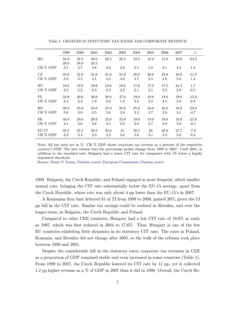
Table 1: CHANGES IN STATUTORY TAX RATES AND CORPORATE REVENUE

1999 2000 2001 2002 2003 2004 2005 2006 2007 4

BG 34.3 32.5 28.0 23.5 23.5 19.5 15.0 15.0 10.0 -24.328.0 28.0 23.5

CR % GDP 3.1 2.7 3.8 3.0 2.8 2.5 1.8 2.1 4.4 1.3

CZ 35.0 31.0 31.0 31.0 31.0 28.0 26.0 24.0 24.0 -11.0CR % GDP 3.8 3.5 4.1 4.3 4.6 4.7 4.5 4.8 5.0 1.2

HU 19.6 19.6 19.6 19.6 19.6 17.6 17.5 17.5 21.3 1.7CR % GDP 2.3 2.2 2.3 2.3 2.2 2.1 2.1 2.3 2.8 0.5

PL 34.0 30.0 28.0 28.0 27.0 19.0 19.0 19.0 19.0 -15.0CR % GDP 2.4 2.4 1.9 2.0 1.8 2.2 2.5 2.4 2.8 0.4

RO 38.0 25.0 25.0 25.0 25.0 25.0 16.0 16.0 16.0 -22.0CR % GDP 3.8 3.0 2.5 2.6 2.8 3.2 2.7 2.8 3.1 -0.7

SK 40.0 29.0 29.0 25.0 25.0 19.0 19.0 19.0 19.0 -21.0CR % GDP 3.1 2.6 2.6 2.5 2.8 2.6 2.7 2.9 3.0 -0.1

EU-17 35.5 35.5 33.8 32.6 31 30.5 29 28.6 27.7 -7.8CR % GDP 3.3 3.4 3.3 3.3 3.0 3.0 3.1 3.3 3.6 0.3

Note: All tax rates are in %. CR % GDP shows corporate tax revenue as a percent of the respectivecountry’s GDP. The last column lists the percentage points change from 1999 to 2007. Until 2001, inaddition to the standard rate, Bulgaria had a lower CIT rate for companies with TI below a legallystipulated threshold.Source: Ernst & Young (Various years); European Commission (Various years)

1999. Bulgaria, the Czech Republic, and Poland engaged in more frequent, albeit smallerannual cuts, bringing the CIT rate substantially below the EU-15 average, apart fromthe Czech Republic, whose rate was only about 4 pp lower than the EU-15’s in 2007.

A Romanian firm that deferred $1 of TI from 1999 to 2000, gained 20%, given the 13pp fall in the CIT rate. Similar tax savings could be realised in Slovakia, and over thelonger-term, in Bulgaria, the Czech Republic and Poland.

Compared to other CEE countries, Hungary had a low CIT rate of 19.6% as earlyas 1997, which was first reduced in 2004 to 17.6%. Thus, Hungary is one of the fewEU countries exhibiting little dynamics in its statutory CIT rate. The rates in Poland,Romania, and Slovakia did not change after 2005, so the bulk of the reforms took placebetween 1999 and 2005.

Despite the considerable fall in the statutory rates, corporate tax revenues in CEEas a proportion of GDP remained stable and even increased in some countries (Table 1).From 1999 to 2007, the Czech Republic lowered its CIT rate by 11 pp, yet it collected1.2 pp higher revenue as a % of GDP in 2007 than it did in 1999. Overall, the Czech Re-

7

public exhibited buoyant and steadily growing corporate tax collections accompanied bygradually declining statutory rate. Revenue was more volatile in Bulgaria. An interestingtrend is that revenue collections dip in the year before a tax cut only to bounce back inthe year of the tax cut. This is valid for the 2000-2001 tax decrease and especially forthe 2006-2007 5 pp cut, which more than doubled revenue in 2007. The same tendencyis observed in Poland, where collections did not change from 1999 to 2000, while the 8pp tax cut from 2003 to 2004 increased revenue. Tax cuts in Romania and Slovakia wereusually followed by a slight drop in revenue, but in general, collections displayed littlefluctuation, remaining especially stable in Hungary.3

3.2 Tax base

In contrast to other EU countries, which broadened the tax base and closed loopholesto make tax cuts revenue-neutral, the six CEE countries considered in this paper nar-rowed their tax bases by introducing various tax incentives and more generous capitalallowances, primarily after 1999.4 Table 2 summarises some of the most important taxincentives, whose effect can later be accounted for in the data.5 In general, most taxbreaks applied to the manufacturing sector, but also overall to businesses operating inareas with high unemployment.

The Czech Republic, for example grants a ten year income tax holiday for companiesinvesting certain funds in manufacturing as well as provides job-creation and retraininggrants. Although few firms qualified for this policy in its starting years, currently manyforeign and domestic investors take advantage of the tax breaks. Other countries choseto stimulate smaller businesses. Romania, for instance, implemented special provisionsfor small and medium enterprises and microenterprises, while Bulgaria offers 100% cor-porate income tax relief if a company operates in a high unemployment region. Besidesmanufacturing, Hungary also supports its hoteling industry and Slovakia has numerousincentives for foreign investors. Since 1995, Poland created seventeen special economiczones (currently fourteen), in which companies can benefit from tax exemptions provided

3It is worth mentioning that the Baltic countries, although not studied in this paper, experienced100% increase in revenue through modest cuts in the CIT rates. From 2000 to 2009, for example, ratesin Estonia and Lithuania fell by 5 and 4 pp, respectively. Collections rose from 0.9% (2000) to 1.8%(2009) in Estonia, and from 0.7% to 1.8% in Lithuania. A similar trend is observed in Latvia.

4In all six countries, indirect taxation is gradually becoming one of the biggest sources of governmentrevenue and certainly of greater importance than the CIT. The shift from direct to indirect taxation isnot limited to CEE, however, and is happening, to a varying degree, across all EU countries. This shiftis acknowledged and in fact encouraged by the European Commission (2010). The increasing relianceon indirect taxes can be a possible explanation of why corporate tax cuts were not accompanied by atax base expansion.

5Except loss carryforward.

8

Tab

le2:

MAJO

RTAX

INCENTIV

ES

BG

2003

Man

ufacturing

compa

nies

qualify

for100%

redu

ctionin

CIT

iflocatedin

mun

icipalities,

whe

reun

employ

mentis

50%

high

erthan

theaverageun

employmentin

thecoun

try.

The

taxis

accoun

tedas

areservean

dshou

ldbe

used

fortheacqu

isitionof

fixed

assets.A

listof

qualify

ingmun

icipalitiesis

publishe

din

CIT

Law

annu

ally.Incentivewas

still

ineff

ectin

2005.Losses

canbe

carriedforw

ardfor5years.

CZ

1999

Corpo

rate

incometaxrelie

ffor10

yearsforfirmsthat

makean

investmentin

aspecified

man

ufacturing

sector,withacertain

portionof

theinvestmentbe

ingcoveredby

equity;inv

estm

entin

machine

rymustaccoun

tforat

least40%

ofthetotalinv

estm

ent.

Incentivewas

still

valid

in2005.Lossescanbe

carriedforw

ardfor7years

2004

Lossescanbe

carriedforw

ardfor5years.

HU

1999

Investmenttaxcred

itof

50%

ofthecorporateincometaxifprod

uctman

ufacturing

investmentof

atleastHUF1billion

ismad

e.Creditcanbe

claimed

ineach

ofthefiv

eyearsfollo

winginvestmentifin

such

yearssalesrevenu

eincreasesby

atleast5%

oftheinvestmentvalue.

Samecond

itions

applyforequivalent

investmentin

theho

telind

ustry,

butsalesturnover

shou

ldincrease

by25%

compa

redto

theprevious

year

butno

tless

than

HUF600million.

Lossescanbe

carriedforw

ardfor5years.

PL

1999

Since1995

Polan

dha

screatedseventeenspecialecono

miczone

s(SEZ).O

nezone

was

sinceclosed

,and

twoweremergedinto

the

Pom

eran

ianSE

Z.Com

panies

canap

plyforpe

rmit

toop

eratein

thesezone

san

dbe

nefit

from

taxexem

ptions

andpreferen

ces.

Tax

exem

ptions

arecalculated

basedon

theam

ount

invested

andthecompa

nywou

ldno

tpa

yincometaxun

tilthe

incometax

exem

ptionlim

itha

sbe

enexha

usted.

RO

2000

Smallan

dmed

ium

enterprises(SMEs)

canredu

cetheircorporateprofi

ttaxby

20%

iftheirem

ploy

mentincreasesby

10%

compa

redto

previous

year.A

SME

isacompa

nywithno

morethan

249em

ployeesan

dan

nual

turnover

less

thane8million.

Thistaxincentivewas

valid

until2

004.

2001

Micro-enterprises

(ME)aretaxedat

1.5%

onsales.

AnME

hasno

morethan

9em

ployeesan

dan

nual

turnover

less

than

e100,000.

Incentivewas

valid

until2

002.

Lossescanbe

carriedforw

ardfor5years.

SKLossescanbe

carriedforw

ardfor5years.

Note:

The

tablelists

only

thosetaxincentives,w

hich

areaccoun

tedfor,giventheda

ta.In

addition

,until2002,B

ulgariaoff

ered

anincentive,

which

redu

ced

profi

ttaxby

10%

oftheam

ountscontribu

tedto

establishacompa

nyor

increase

thecapitalo

facompa

ny,ifthe

amou

ntsareused

toim

provefix

edtang

ible

assets

andtheinvestmentis

mad

ein

mun

icipalitieswith1.5times

high

erun

employ

mentthan

theaverageforthecoun

try.

Besides

acorporateincometax

holid

ay,firmsin

theCzech

Rep

ublic

canalso

applyforjob-creation

gran

ts,custom

s-relatedbe

nefits,

gran

tsforretraining

employeesan

dprop

erty-related

incentives,a

llof

which

canaff

ecttaxa

bleincome.

Hun

gary

addition

ally

offerstaxincentives

foroff

shorecompa

nies.Rom

ania

hasspecialp

rovision

sin

place

forfirmsin

Disfavoured

Econo

mic

Zone

san

dIndu

strial

Parks

(usually

VAT

deferral)an

dlik

ePolan

d,ha

screatedFree-Trade

Zone

sbe

nefitingfrom

5%profi

ttaxrate

oragene

ralprofi

ttaxexem

ption.

Tax

holid

aysan

dtaxcred

itsas

wellas

contribu

tion

sforne

wjobs

andtraining

areavailableto

firmsin

Slovak

ia,althou

ghthey

need

tomeetalong

listof

requ

irem

ents

inorde

rto

qualify

.Colum

n(2)show

stheyear

ofim

plem

entation

ofthetaxincentiveor

theyear

inwhich

analread

yexisting

policywas

mod

ified

.So

urce:Ernst

&You

ng(V

arious

years),U

nitedNations

(2000),K

PMG

Polan

d(2009).

Tab

le3:

CAPIT

ALALLOWANCES

BG

1999-2001

Straight-line

metho

d.I.

Indu

strial

build

ings

andinstallation

s4%

;II.Machine

s,equipm

entan

dap

pliances,offi

ceequipm

ent

20%;III.V

ehiclesan

dothe

rtype

sof

tran

sportation

(excl.

automob

iles)

8%;IV.A

llothe

rassets

15%

2002

Forassets

inGroup

IIan

dcertainassets

inGroup

I,acceleratedde

preciation

ofup

to30%

allowed

.2003-2005

I.Buildings,facilities,e

tc.4%

;II.Machine

s,man

ufacturing

equipm

ent,ap

paratus30%

(can

beincreasedto

upto

50%

forne

winvestments

inlong

-term

assets);

III.

Transpo

rtationvehicles,excl.au

tomob

iles10%;IV

.Com

puters

andsoftware50%;V.

Autom

obile

s25%;V

I.Other

tang

ible

assets

15%;V

II.Intan

gibleassets

–max

imum

rate

25%.Dep

ends

onpe

riod

ofuse.

CZ

1999-2004

Cho

iceof

straight

lineor

acceleratedde

preciation

.I.Passeng

ercars,bu

ses,

light

machine

ry4years(straigh

tlin

e)14.2%

first

year

28.6%

subseque

ntyears,(accelerated

)4first

year,5

subseque

nt;II.Airplan

es,furniture,e

tc.6years8.5%

first

year

18.3%

subseque

ntyears,

(accelerated

)6first

year,7subseque

nt;III.

Heavy

machine

ry12

years(straigh

tlin

e)4.3%

first

year

8.7%

subseque

ntyears,(accelerated

)12

first

year,1

3subseque

nt;IV.W

oode

nbu

ildings,p

ipelines,e

tc.20

years(straigh

tlin

e)2.15%

first

year

5.15%

subseque

ntyears,(accelerated

)20

first

year,2

1subseque

nt;V

.Allothe

rbu

ildings

30years(straigh

tlin

e)1.4%

first

year

3.4%

subseque

ntyears,(accelerated

)30

first

year,3

1subseque

nt.Tan

gibleassets

valued

atup

toCZK

40,000

canbe

dedu

cedim

med

iately.10%

initialde

preciation

allowan

ceforcertainassets

ifcompa

nyis

first

owne

r.15%

initialde

preciation

allowan

ceforpu

rificationan

dprocessing

ofwater

equipm

ent.

20%

allowan

ceforcertainagricultural

equipm

ent.

2004

VI.Sp

ecified

build

ings

50years(straigh

tlin

e)1.02%

first

year

2.02%

subseque

ntyears,(accelerated

)50

first

year,5

1subseque

nt.

Intang

ible

assets

divide

dinto

twocategories

depe

ndingon

period

ofuse.

Intang

ible

assets

upto

CZK

60,000

canbe

dedu

cted

immed

iately.

2005

Highe

rde

preciation

ratesforoffi

cemachine

s,Busses,

airplane

s,tractors,lorries

andfurniture,

andhe

avymachine

ry.

HU

1999-2005

Straight-line

depreciation

.I.

Hotel

and

catering

build

ings

3%;II.Indu

strial

and

commercial

build

ings

2to

6%III.

Motor

vehicles

20%;IV

.14.5%

(Com

puters,au

tomationequipm

ent,

etc.

33%).

Various

equipm

entvalued

atless

than

HUF

100,000

canbe

written

offover

twoyears.

2004

V.C

ompu

ters

50%.

2005

VI.Intelle

ctua

lprope

rtyan

dfilm

prod

uction

equipm

ent50%.

PL

1999-2005

Straight-line

metho

d.In

certaincasesde

cliningba

lancecanbe

allowed

.Fo

rcertainassets

(machine

ry),

depreciation

ratescan

bedo

ubled.

Com

panies

inhigh

unem

ploy

mentaresubjectto

morefavourab

letaxde

preciation

.I.

Buildings

1.5to

10%;II.

Office

equipm

ent14%;III.C

ompu

ters

30%;IV.M

otor

vehicles

14to

20%;V

.Plant

andmachine

ry5to

20%.

2005

30%

depreciation

rate

forcertainne

wfix

edassets.

RO

1999-2001

Straight-line

metho

d.I.Buildings

andconstruction

s10

to50

years;

II.Machine

ryan

dequipm

ent4to

10years;

III.Fu

rniture

andfitting

s5to

10years;

Motor

vehicles

5to

9years.

Assetsmay

berevalued

annu

ally

ifcumulativeinfla

tion

rate

forlast

3yearsexceed

s100%

.2002

Accelerated

depreciation

canbe

claimed

subjectto

certaincriteria.

2003-2005

Accelerated

depreciation

fortechno

logicalequipm

ent,

machine

ries,tools,

installation

s,compu

ters

andpe

riph

eral

equipm

ent,

unde

rwhich

assets

canbe

depreciatedat

50%

rate

intheyear

ofpu

rcha

seor

20%

dedu

ctionforinvestments

inde

preciablefix

edassets

ifacceleratedde

preciation

isno

tselected

asan

option

.

SK1999-2003

Cho

iceof

straight

lineor

acceleratedde

preciation

.I.Passeng

ercars,bu

ses,

light

machine

ry4years(straigh

tlin

e)14.2%

first

year

28.6%

subseque

ntyears,

(accelerated

)4first

year,5subseque

nt;II.Airplan

es,offi

ceequipm

ent,

etc.

8years6.2%

first

year

13.4%

subseque

ntyears,(accelerated

)8first

year,9

subseque

nt;III.H

eavy

machine

ryan

dpa

tents15

years(straigh

tlin

e)3.4%

first

year

6.9%

subseque

ntyears,(accelerated

)15

first

year,1

6subseque

nt;IV.W

oode

nbu

ildings,p

ipelines,e

tc.30

years

(straigh

tlin

e)1.4%

first

year

3.4%

subseque

ntyears,

(accelerated

)30

first

year,3

1subseque

nt;V

.Allothe

rbu

ildings

40years

(straigh

tlin

e)1.5%

first

year

2.5%

subseque

ntyears,

(accelerated

)40

first

year,4

1subseque

nt.

2000

Intang

ible

assets

depreciatedforape

riod

of2bu

tno

tmorethan

5years.

2004-2005

Four

categories

ofassets

butratesan

dyearsareno

tlisted.

Source:Ernst

&You

ng(V

arious

years).

they obtain a permit from the zoning authorities.Table 2 and Appendix A.2 describe thetax incentives in greater detail.

With regard to capital allowances, all six countries maintained the yearly write-down allowances at their 1999 level (Table 3). Gradually, more detailed asset categorieswere introduced that generally benefited from higher depreciation rates, a developmentapplying especially to the IT and communications sector. Provisions for intangible assetswere also established. In 2003 Bulgaria increased the depreciation rates for some assetsincluding plant and machinery, followed by the Czech Republic in 2005. Romania allowedfor an accelerated depreciation rate at 50% in the year of purchase for technologicalequipment and other machinery in service after 2002.

Due to the limitations of the data, a single definition of taxable income cannot beadopted in the empirical analysis that follows. It is therefore important to establish thatthe definition of TI has not changed in such a way that TI would have grown for reasonsunrelated to tax rates or firms’ profitability.

While the definition of taxable income was indeed altered in all countries, it wasmostly in the direction of increasing deductible expenses. In Bulgaria, the number ofnew provisions reducing the financial result was far greater than the ones raising it. Thelist of deductible expenses in Hungary, Poland and the Czech Republic remained virtuallythe same, with the exception of a new provision introduced in 2004 in the Czech Republic,stipulating that the purchase cost of intangible assets up to CZK60,000 can be deductedimmediately (Ernst & Young, Various years). Romania followed a balanced approachin modifying firms’ taxable income. For example, up to 1.5% of total salary cost couldbe deducted in 2005 compared to 2% in 2004, but in 2005 permanent establishmentscould deduct R&D, and management and administration expenses up to 10% of taxablesalaries.

Given the described policies and the falling CIT rates, the strength of corporate taxrevenues cannot be explained by expansions in the tax base. It is certainly possible,however, that enhancement of tax administrations’ enforcement and collection abilitiescould have generated additional revenue by driving more firms out of the shadow econ-omy. According to the World Bank Worldwide Governance Indicators, regulatory quality,which incorporates the effectiveness of the tax collection system, has improved tremen-dously in CEE for the period 1999-2005. Nevertheless, according to the indicators, thereare mixed signals concerning the control of corruption, which has not exhibited markedadvancement, and in the case of Poland, has actually worsened with time.

11

3.3 Rate of incorporation and profitability

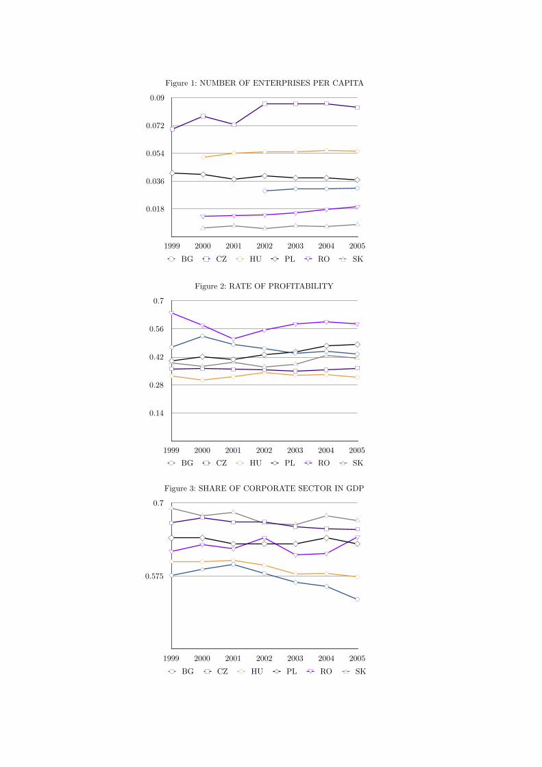
Even if the tax base became narrower, lower CIT rates could have promoted a higherrate of incorporation and the growth of already established businesses. Further, firmsmay have become more profitable due to non-tax reasons. To examine if this is thecase, I study changes in the profit rate of corporations, the share of the corporate sectorin GDP and the number of firms per capita. I follow Clausing (2007) and construct arate of profitability measure by dividing corporations’ aggregate net operating surplusby corporate value added. Corporate value added scaled by GDP serves as a measureof the share of the corporate sector. Finally, the number of firms by industry as well aspopulation statistics are taken from OECD’s Structural Business Statistics and Eurostat.

Figure 1 shows the number of enterprises per capita in the non-financial sector from1999 to 2005. The number of firms relative to the population increased in Romaniaand remained virtually unchanged in Hungary, Slovakia, and Bulgaria. There was asubstantial jump in the entry of firms in the Czech Republic between 2001 and 2002, withthe time series stabilising at the higher level post 2002.6 In general, the Czech Republichas markedly higher businesses-to-population ratio than the remaining five countries. Incontrast, Poland experienced an overall decline in businesses both in absolute and percapita level.

Trends in profitability are depicted in Figure 2. Looking in more detail at the sectoraldifferences, the mining and quarrying as well as the electricity, gas, and water supply in-dustries expanded in all countries, although their profitability was volatile – from negativein Poland, Slovakia and Hungary to steadily growing in the Czech Republic (AppendixA.1: Tables 11 and 12).7 The number of firms operating in the Real Estate and BusinessServices sector grew in all countries and its profitability remained stable.

Apart from the sectors mentioned above, the number of enterprises in Poland declinedin all other industries, yet their profitability increased considerably. Piotrowska andVanborren (2008) also find an increasing entry rate and corporate profit share for theCzech Republic and Poland, respectively. Overall, only Poland and Slovakia exhibit anupward tendency in the rate of profitability.8 Last but not least, the share of the corporatesector in GDP declined in Bulgaria, Hungary, and Slovakia, remained the same in Polandand the Czech Republic, and increased in Romania, as depicted in Figure 3.

6The entry rate could have been even higher as the change of the number of firms from one year tothe next is a combination of both the birth and death rates of firms.

7For Romania, the data is only for the total number of firms.8Figure 2 excludes the financial sector, but the trends do not change if this sector is considered.

12

0.018

0.036

0.054

0.072

0.09

1999 2000 2001 2002 2003 2004 2005

Figure 1: NUMBER OF ENTERPRISES PER CAPITA

BG CZ HU PL RO SK

0.14

0.28

0.42

0.56

0.7

1999 2000 2001 2002 2003 2004 2005

Figure 2: RATE OF PROFITABILITY

BG CZ HU PL RO SK

0.575

0.7

1999 2000 2001 2002 2003 2004 2005

Figure 3: SHARE OF CORPORATE SECTOR IN GDP

BG CZ HU PL RO SK

4 Empirical Analysis

4.1 Data

I use firm-level panel data from the comprehensive AMADEUS dataset for Europeancompanies compiled by Bureau van Dijk. The data consists of financial statements’variables as reported by firms. I consider data for the 6 CEE countries discussed above,namely Bulgaria, the Czech Republic, Hungary, Poland, Romania, and Slovakia for theperiod 1999-2005. Earlier years are not included because AMADEUS’s data coverage forCEE was limited before and even in 1999 and also because most tax reforms took placeafter 1999.

Sole proprietors, partnerships, societies, associations and non-profit organisations areexcluded from the analysis, since some are non-corporate entities and others are subjectto special tax provisions. For each country I keep public and private limited companies,branches of foreign corporations, as well as municipal and state companies, resulting ina dataset of 3,248,643 firm-year observations. If a firm has submitted both consolidatedand unconsolidated statements, only the unconsolidated statement is considered in orderto avoid repetitive firm observations (3,795 firm-year observations dropped). The sam-ple is further restricted to include firms whose status is active, i.e., not in bankruptcy,dissolution, or liquidation, and that file a report at the end of the year (11,399 firm-yearobservations dropped).

I follow Klapper et al. (2006) and Da Rin et al. (2011) and exclude certain industriesthat are unlikely to manage taxable income or are subject to stricter regulations. In par-ticular, I remove financial services (NACE2 65-66; 2,551 firm-year observations), publicadministration, education, and other social and personal services industries (NACE2 75,80, 90, 91, 92, 95, 97, 99; 40,328 firm-year observations) as well as firms missing anindustry classification (36,471 firm-year observations). Overall, there remain 51 differentindustries based on a NACE2 classification. I additionally drop observations with spellsof missing values of taxes paid, cost of employees, profit/loss for the period and depreci-ation in the beginning and the end of each panel (1,112,893 firm-year observations), allof which are variables used later on in the calculation of effective tax rates.

All financial amounts are transformed into thousands of USD using AMADEUS’sexchange rate from the local currency to USD at the fiscal year end of companies. Byand large, the exchange rates exhibit little volatility, which will not affect the subsequentempirical estimation as all balance-sheet variables are scaled by total assets. Thestatutory tax rates for each country are described in Table 1, but before proceeding withcomputing taxable income, I need to identify firms that have utilised tax breaks, and

14

therefore face lower or zero corporate tax rates. In the data, such firms usually appearas paying zero taxes due to tax incentives, yet it would be wrong to infer their taxableincomes to be zero.

Appendix A.2 describes in detail what types of firms qualify for tax incentives andhow they are identified. All in all, approximately 600 major manufacturing firms fromBulgaria, the Czech Republic, Hungary and Poland qualify for some tax incentive. Thenumber is much more substantial for Romania, since the incentives cover SMEs andmicroenterprises. About 9,000 companies per year (2000-2004) in Romania fulfil theSMEs incentive criteria and more than 70,000 firms in 2001 could use the microenterprisestax rate. Earnings before interest and tax (ebit) are used as a measure of taxable incomein the case of a tax incentive, which enables the firm to pay no tax. If the incentivereduces the tax rate, then I simply assign the lower rate to the eligible firm.

4.2 Computing firm-level effective tax rates

The methodology of Devereux and Griffith (2003) is followed to compute effective averagecorporate tax rates (EATR) based on the net-present value (NPV) of a hypotheticalinvestment project, calculated in the presence and absence of a tax. In particular,

EATR =R∗ −RR∗

, (1)

with R∗ being the NPV of the project without tax and R – the NPV with tax. Anattractive feature of this effective tax rate, as pointed out by Devereux and Griffith(2003), is that it constitutes a weighted average of the marginal effective tax rate formarginal investments, and the statutory tax rate for very profitable investments. R isderived in the following way: If Vt is the market value of a firm’s shares, then followingKing (1974), the net-of-tax yield from investing Vt at the market rate of interest mustequal the net-of-tax dividends, Dt, plus the capital gain in order to achieve equilibriumin the capital market

it(1−mit)Vt =

1−mdt

1− ctDt + (1− zt)(Vt+1 − Vt −Nt), (2)

where it is the market rate of interest at time t, mit is the personal tax rate on interest

income, mdt is the tax rate on dividend income, zt is the capital gains’ tax rate, ct is the

rate of tax credit on dividends, and Nt is the new equity issued.Solving this difference equation and assuming a one unit increase in the capital stock

15

in period t dKt = 1, which is reduced in the next period so that dKk = 0 ∀ k 6= t,

yields a change in the value of the firm R = dVt =∑∞

k=0

[θdDt+k−dNt+k

(1+ρ)k

], where θ =

(1−mdt )/(1− ct)(1− zt) and ρ = (1−mi

t)it/(1− zt).From the equation for the appropriation of income, one obtainsDt asDt = Y (Kt−1)(1−

τ st ) − It + Bt − (1 + it(1 − τ st ))Bt−1 + τ st φt(I + KTt−1) + Nt. Output Y in period t is a

function of the beginning of year capital stock Kt−1, τ st is the statutory corporate taxrate, It is investment, Bt is debt, with interest payments assumed to be tax-deductible,φt is the depreciation rate of capital, and KT

t−1 is defined as tax-written-down value ofcapital stock at the beginning of t (Devereux and Griffith, 2003). Deriving the changein dDt+k from the equation for Dt and plugging into the equation for dVt, Devereux andGriffith (2003) obtain R and subsequently the EATR for different sources of financing.

Throughout this paper I assume that θ = 1, i.e., mdt = ct = zt = 0. Additionally, I

assume that mit = 0, which leads to the nominal discount rate of shareholders ρ = i. θ

was first defined by King (1974) as a measure of the degree of discrimination betweenretaining profits and distributing profits as dividends. In other words, if paying dividendsgenerates more tax liability as compared to retaining earnings, then θ < 1. Therefore,assuming that θ = 1, or equivalently not considering personal income taxes, implies thatfinancing projects either by retained earnings, or the issue of new shares yields the sameEATR.

Based on the assumptions above,

R =1

1 + i[(p+ δ)(1 + π)(1− τ s)− ((1 + i)− (1− δ)(1 + π))(1−A)] + F, (3)

where the first term in brackets is the net-of-tax change in output caused by a one unitincrease in the capital stock, with p being the real financial return, δ one period costof depreciation and π the inflation rate, which is the same for capital and output. Thesecond term in brackets is the required decrease in investment to keep capital stockunchanged in period t + 1. A is the NPV of tax allowances per unit of investment andF is the cost of raising external finance.9

Provided that the investment is financed by debt, because of deductible interestpayments, taxable income will be lower, and hence the EATR is smaller. To see this,note that if the firm borrows 1 − φτ in period t, then R incorporates the amount ofdeductible interest payments F = iτ s 1−φτ

s

1+i , which leads to a lower EATR as compared

9For θ = 1 and ρ = i, A = φτs (1+i)i

(1− 1

(1+i)T+1

), where T = 1/φ for straight-line depreciation, and

A = φτs (1+i)(i+φ)

for declining balance. See also Da Rin et al. (2011).

16

to the case when F = 0, which is equivalent to financing by retained earnings or equity.10

Correspondingly, R∗ is simply R without the taxes, or

R∗ = −1 +1

1 + i[(p+ δ)(1 + π) + (1− δ)(1 + π)] =

p− r1 + r

(4)

using the relationship between the real r and nominal i interest rates (1 + r)(1 + π) =

(1 + i). The difference R∗ − R is then scaled by the NPV of the pre-tax total incomestream net of depreciation p/(1 + r) in order to obtain a measure of the EATR (SeeAppendix A.3).

Similarly to Da Rin et al. (2011), I measure the nominal interest rate i with the rateof short-term government bonds. In particular, two-year government bond rates are usedfor Bulgaria, Poland and Slovakia, and one-year government bond and one year treasurybill rates for the Czech Republic and Hungary, respectively. No such rate is availablefor Romania, so it is approximated with the money market interested rate, taken fromEurostat. I use the Harmonized Indices of Consumer Prices from Eurostat as a measureof the inflation rate π.

The maximum depreciation rates for plant and machinery in the cases of Polandand Hungary, heavy machinery for the Czech Republic and Slovakia, and machines andmanufacturing equipment for Bulgaria and Romania are used as the rates at which capitalexpenditure is offset against tax φ. The results presented below are robust to using otherasset categories’ depreciation rates and the average of these.

The financial rate of return p is obtained by subtracting expenditures on employees(staf) from the added value (av), and dividing this difference by the added value: (av−staf)/av, where in AMADEUS av is defined as the sum of taxes paid (taxa), profit/lossfor the period (pl), depreciation (depre), interest paid (inte), and labour expenses (staf).Da Rin et al. (2011) employ an identical measure but on an industry level.

A major problem is that about 90% of the AMADEUS firms have missing values forinterest paid. For this reason, p is calculated without including this variable. However,estimates are presented for the small sample of firms who have reported interest payments,with p calculated accordingly, with the results confirming income shifting, although thenon-transitory responses tend to be lower (close to zero) than the long-term responsesestimated without inte.

All remaining variables, namely r, A, R and R∗ are calculated using the formulasdescribed above. The one-period cost of depreciation δ is assumed to take a value of12.5%, taken from Da Rin et al. (2011). A step-by-step explanation of the variables and

10The assumption is that the firm is eligible for an immediate tax allowance of φτs, hence 1− φτs.

17

formulas used to calculate the EATR is provided in Appendix A.3.

4.3 Taxable income

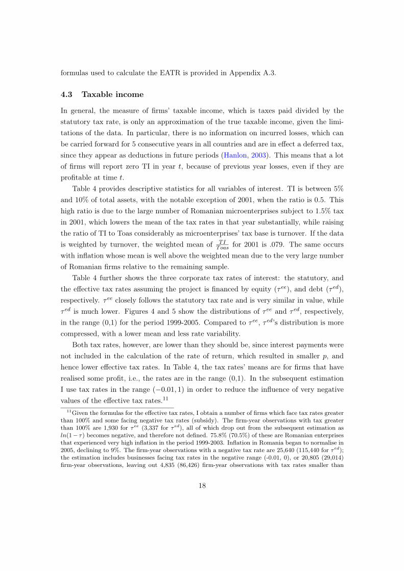
In general, the measure of firms’ taxable income, which is taxes paid divided by thestatutory tax rate, is only an approximation of the true taxable income, given the limi-tations of the data. In particular, there is no information on incurred losses, which canbe carried forward for 5 consecutive years in all countries and are in effect a deferred tax,since they appear as deductions in future periods (Hanlon, 2003). This means that a lotof firms will report zero TI in year t, because of previous year losses, even if they areprofitable at time t.

Table 4 provides descriptive statistics for all variables of interest. TI is between 5%and 10% of total assets, with the notable exception of 2001, when the ratio is 0.5. Thishigh ratio is due to the large number of Romanian microenterprises subject to 1.5% taxin 2001, which lowers the mean of the tax rates in that year substantially, while raisingthe ratio of TI to Toas considerably as microenterprises’ tax base is turnover. If the datais weighted by turnover, the weighted mean of TI

Toas for 2001 is .079. The same occurswith inflation whose mean is well above the weighted mean due to the very large numberof Romanian firms relative to the remaining sample.

Table 4 further shows the three corporate tax rates of interest: the statutory, andthe effective tax rates assuming the project is financed by equity (τ ee), and debt (τ ed),respectively. τ ee closely follows the statutory tax rate and is very similar in value, whileτ ed is much lower. Figures 4 and 5 show the distributions of τ ee and τ ed, respectively,in the range (0,1) for the period 1999-2005. Compared to τ ee, τ ed’s distribution is morecompressed, with a lower mean and less rate variability.

Both tax rates, however, are lower than they should be, since interest payments werenot included in the calculation of the rate of return, which resulted in smaller p, andhence lower effective tax rates. In Table 4, the tax rates’ means are for firms that haverealised some profit, i.e., the rates are in the range (0,1). In the subsequent estimationI use tax rates in the range (−0.01, 1) in order to reduce the influence of very negativevalues of the effective tax rates.11

11Given the formulas for the effective tax rates, I obtain a number of firms which face tax rates greaterthan 100% and some facing negative tax rates (subsidy). The firm-year observations with tax greaterthan 100% are 1,930 for τee (3,337 for τed), all of which drop out from the subsequent estimation asln(1− τ) becomes negative, and therefore not defined. 75.8% (70.5%) of these are Romanian enterprisesthat experienced very high inflation in the period 1999-2003. Inflation in Romania began to normalise in2005, declining to 9%. The firm-year observations with a negative tax rate are 25,640 (115,440 for τed);the estimation includes businesses facing tax rates in the negative range (-0.01, 0), or 20,805 (29,014)firm-year observations, leaving out 4,835 (86,426) firm-year observations with tax rates smaller than

18

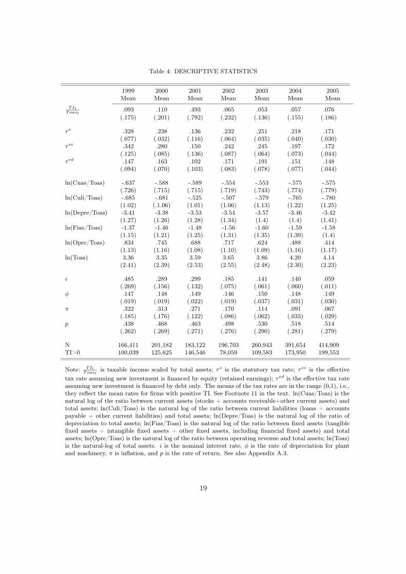
Table 4: DESCRIPTIVE STATISTICS

1999Mean

2000Mean

2001Mean

2002Mean

2003Mean

2004Mean

2005Mean

TItToast

.093 .110 .493 .065 .053 .057 .076(.175) (.201) (.792) (.232) (.136) (.155) (.186)

τs .328 .238 .136 .232 .251 .218 .171(.077) (.032) (.116) (.064) (.035) (.040) (.030)

τee .342 .280 .150 .242 .245 .197 .172(.125) (.085) (.136) (.087) (.064) (.073) (.044)

τed .147 .163 .102 .171 .191 .151 .148(.094) (.070) (.103) (.083) (.078) (.077) (.044)

ln(Cuas/Toas) -.637 -.588 -.589 -.554 -.553 -.575 -.575(.726) (.715) (.715) (.719) (.743) (.774) (.779)

ln(Culi/Toas) -.685 -.681 -.525 -.507 -.579 -.765 -.780(1.02) (.1.06) (1.01) (1.06) (1.13) (1.22) (1.25)

ln(Depre/Toas) -3.41 -3.38 -3.53 -3.54 -3.57 -3.46 -3.42(1.27) (1.26) (1.28) (1.34) (1.4) (1.4) (1.41)

ln(Fias/Toas) -1.37 -1.46 -1.48 -1.56 -1.60 -1.59 -1.58(1.15) (1.21) (1.25) (1.31) (1.35) (1.39) (1.4)

ln(Opre/Toas) .834 .745 .688 .717 .624 .488 .414(1.13) (1.16) (1.08) (1.10) (1.09) (1.16) (1.17)

ln(Toas) 3.36 3.35 3.59 3.65 3.86 4.20 4.14(2.41) (2.39) (2.53) (2.55) (2.48) (2.30) (2.23)

i .485 .289 .299 .185 .141 .140 .059(.269) (.156) (.132) (.075) (.061) (.060) (.011)

φ .147 .148 .149 .146 .150 .148 .149(.019) (.019) (.022) (.019) (.037) (.031) (.030)

π .322 .313 .271 .170 .114 .091 .067(.185) (.176) (.122) (.086) (.062) (.033) (.029)

p .438 .468 .463 .498 .530 .518 .514(.262) (.269) (.271) (.276) (.290) (.281) (.279)

N 166,411 201,182 183,122 196,703 260,943 391,654 414,909TI>0 100,039 125,625 146,546 78,059 109,583 173,950 199,553

Note: TItToast

is taxable income scaled by total assets; τs is the statutory tax rate; τee is the effectivetax rate assuming new investment is financed by equity (retained earnings); τed is the effective tax rateassuming new investment is financed by debt only. The means of the tax rates are in the range (0,1), i.e.,they reflect the mean rates for firms with positive TI. See Footnote 11 in the text. ln(Cuas/Toas) is thenatural log of the ratio between current assets (stocks + accounts receivable+other current assets) andtotal assets; ln(Culi/Toas) is the natural log of the ratio between current liabilities (loans + accountspayable + other current liabilities) and total assets; ln(Depre/Toas) is the natural log of the ratio ofdepreciation to total assets; ln(Fias/Toas) is the natural log of the ratio between fixed assets (tangiblefixed assets + intangible fixed assets + other fixed assets, including financial fixed assets) and totalassets; ln(Opre/Toas) is the natural log of the ratio between operating revenue and total assets; ln(Toas)is the natural-log of total assets. i is the nominal interest rate, φ is the rate of depreciation for plantand machinery, π is inflation, and p is the rate of return. See also Appendix A.3.

19

02

46

8D

ensit

y

0 .2 .4 .6 .8 1τee

Figure 4: EFFECTIVE AVERAGE CORPORATE TAX RATES, EQUITY: 1999-20050

24

68

10D

ensit

y

0 .2 .4 .6 .8 1τed

Figure 5: EFFECTIVE AVERAGE CORORATE TAX RATES, DEBT: 1999-2005

Unlike Western European countries, where the average inflation for the period 1999-2005 was about 3%, CEE had high rates of inflation, especially in the period 1999-2002,which normalised to about 7%, on average, in 2005. The nominal interest rates reflectthe high inflation rates and also decrease over time.

4.4 Methodology

The goal is to separate the long-run and short-run responses of taxable income to changesin the tax rates and this involves taking account of income shifting by firms in anticipationof lower future rates. To separate the responses, I employ the following specification:

TIitToasit

= αi + β1[ln(1− τ eit)− ln(1− τ eit−1)] + β2ln(1− τ eit)

+ β3[ln(1− τ eit+1)− ln(1− τ eit)] + εit (5)

= αi + (β1 + β2 − β3)ln(1− τ eit)− β1ln(1− τit−1) + β3ln(1− τit+1) + εit

which is similar to the one used by Heim (2006) and Goolsbee (2000). TIit is thetaxable income of firm i in year t scaled by total assets Toas. ln(1− τ eit−1), ln(1− τ eit),and ln(1 − τ eit+1) are the natural logarithms of the lagged, the contemporaneous, andthe leading net-of-EATR shares, respectively, and αi are firm fixed effects. αi captureunobserved heterogeneity for firm i, assuming that firms differ randomly in a way that isnot completely controlled for by the observed covariates (Cameron and Trivedi, 2009a).In this specification, TI

Toas in period t is affected not only by the current tax rate, butalso by the difference between the current and lagged and current and leading rates.

If τ et−1 > τ et > τ et+1, I expect firms to shift income out of year t − 1 into the currentyear t, and again, out of year t into t + 1. Let τ et−1 − τ et = 4τ e. Then deferring $1 ofTI to year t translates into gaining 4τe

1−τet−1. Thus, the effect of ln(1 − τ eit−1) on taxable

income in the current year, TIt, is likely to be positive (β1 > 0), and that of ln(1− τ eit+1)

– negative (β3 < 0). The coefficient of the current net-of-tax share is a combination ofthe current effect and two shifting coefficients, which entails the explicit control for the

-1%. It is worth pointing out that more than 60% of all firms with negative tax rates belong to a narrowcategory of firms, which are also the most difficult to tax, namely: General construction and plumbing;restaurants and bars; sale, maintenance and repair of motor vehicles; sales agents; and retail trade withfood, beverages and tobacco predominant. Last but not least, the firm-year observations facing a zeroeffective tax rate are 862,694 for both τee and τed, or approximately 47% of the whole sample. Again,more than 63% of the firms with zero effective tax rates belong to NACE2: 45, 50, 51, 52, and 55,i.e., construction, wholesale and retail trade and hotels and restaurants, and to NACE2 74, which isaccounting and tax consulting services.

21

lagged and leading shares, if β2 = (β1 + β2 − β3)− β1 + β3, the long-run effect, is to beestimated consistently.

In the linear-log specification, the coefficients measure the absolute change in TIitToasit

for a relative change in the net-of-tax shares, so that a 1% increase in ln(1 − τit+1),increases the ratio of TI to total assets by β3/100, where the division comes from theswitch from relative to percentage change. The reason why I cannot log-transform thedependent variable is that such transformation turns observations with zero taxable in-come into missing values, thus creating gaps in the individual firm-panels as log(0) is notdefined.

If I log-transform, the estimation will be based solely on firms that have reportedpositive taxable incomes. Therefore, the dependent variable is no longer E[ln(TI)] butE[ln(TI)|x, TI > 0]. Without the log-transformation, there is a mass point of TI atzero, but not a problem with observability of the dependent variable. In other words, thezeros in the case of firms’ taxable income are not due to self-selection but are an actualoutcome value. For this reason self-selection models are not appropriate for the data,while if Tobit is used, I need to assume random effects and even then, differencing thedata to eliminate the firm-effects can lead to complications.12

There are several problems with the specification as presented above. First, ln(1−τ eit)is endogenous in (5) not only due to spurious correlation stemming from the fact thatcommon factors, such as taxes paid taxa and the statutory tax rate τ s, determine bothTIit and the effective tax rate τ eit, but also due to reverse causality. For example, in thecase of firms that sustain losses, it is TI that determines the tax rate. Similarly, smallerfirms can be taxed at preferential rates, provided that their TI do not exceed a certainlimit.

Second, even if a suitable instrumental variable (IV) for ln(1 − τ eit) is available, anadditional problem arises due to the dynamic nature of the specification and the as-sumption that the fixed-effects αi are correlated with the observed regressors xit, whichnecessitates αi’s elimination through the transformation of the data. In particular, notethat a fixed-effects, two-stage least square estimation of (5) will lead to an inconsistentfirst stage. The first stage is an OLS of the demeaned data:

ln(1− τ eit)− ln(1− τ ei ). = γ0 + γ1(IVit − IVi.) + γ2[ln(1− τ eit−1)− ln(1− τ ei )−1]

+ γ3[ln(1− τ eit+1)− ln(1− τ ei )+1] + εit − ε̄i., (6)

12See Kalwij (2003) for more details on Tobit in first-differences with individual effects. Since taxableincome is zero when a loss is realised, it is in fact a censored variable, so that: TIit = TI∗it if TI∗it > 0(taxable profit is realised) and TIit = 0 if TI∗it ≤ 0 (taxable loss or the firm breaks even).

22

where ln(1− τ ei ). = T−1i

∑t=Tit=1 ln(1 − τit), ln(1− τ ei )−1 = T−1i

∑t=Ti−1t=0 ln(1 − τit),

and ln(1− τ ei )+1 = T−1i

∑t=Ti+1t=2 ln(1 − τit). This regression would lead to inconsis-

tent parameter estimates, because ln(1− τ eit−1) and −T−1i ln(1− τ eit) are correlated with−T−1i εit−1 and εit, respectively. Similar negative correlations occur for the leading net-of-tax share, yielding an inconsistent within estimator (Bond, 2002). For a single lagged de-pendent variable, Nickell (1981) demonstrates that the leading negative correlations out-weigh the positive correlations between terms such as −T−1i εit−1 and −T−1i ln(1− τit−1),resulting in downward bias in γ2. Eq.(6), however, contains a second endogenous vari-able, making it unclear if the bias formulas hold in this case. In fact, an IV estimation inthe presence of any lagged or leading terms in levels will produce an inconsistent within-estimator (Cameron and Trivedi, 2009b). Therefore, in order to remove αi and estimateeq.(6), and therefore eq.(5) consistently, I turn to the first-difference estimator.

An important advantage of the first-differencing transformation is that, unlike de-meaning, it does not introduce all realisations of the disturbances (εi1, εi2, ...εiT ) into thetransformed error term. Nevertheless, adjacent time periods are still problematic. Notethat in the first-differenced first stage of (5)

ln

(1− τ eit+1

1− τ eit

)= θ0 + θ14IVit+1 + θ2ln

(1−τeit

1−τeit−1

)+ θ3ln

(1−τeit+2

1−τeit+1

)+4εit+1, (7)

4εit+1 is correlated with ln

(1−τeit

1−τeit−1

)and

(1−τeit+2

1−τeit+1

), since ln(1 − τ eit) and −ln(1 −

τ eit+1) are correlated with −εit and εit+1, respectively, leading to a downward bias. Itis uncertain how the bias in the case of first differencing will compare to demeaningconsidering the second endogenous regressor. ln(1 − τ eit−k), for k ≥ 2, however, is notcorrelated with the error term, which opens up the possibility for consistent estimationusing a longer difference window. Specifically a two year window is considered, so that(5) becomes

TIit+2

Toasit+2− TIitToasit

= λt + λjt + λct + σ1ln

(1− τ eit+2

1− τ eit

)− σ2ln

(1− τ eit+1

1− τ eit−1

)+ σ3ln

(1− τ eit+3

1− τ eit+1

)+4X ′Γ + εit+2 − εit, (8)

which will result in a consistent first stage of the 2SLS, provided that two key assumptionsare met: εit are independent across firms and εit are serially uncorrelated.

λt, λjt, λct are year, industry-year (NACE2 level) and country-year dummies, respec-

23

tively; X includes the natural logarithm of the ratios of current assets, current liabilities,depreciation, fixed assets, and operating revenue to total assets as well as the natural logof total assets.

As explained above, eq.(8) requires an IV for the contemporaneous change in the net-

of-tax shares ln(

1−τeit+2

1−τeit

). Using Gruber and Rauh (2007)’s methodology, I construct

an instrument by calculating the EATR in year t+ 2 with the firm characteristics fromyear t. Specifically, I keep the added value av at its year t level and inflate it by theproducer price index, but allow the macroeconomic variables, such as the statutory taxrate, depreciation rules, etc., to change. The idea is to make the change in the net-of-taxshares between year t and t+2 exogenous to firm behaviour by removing that componentof the change, which can be driven by tax planning considerations. The instrument for

ln

(1−τeit+2

1−τeit

)is therefore ln

(1−τpit+2

1−τeit

), where 1−τpit+2 is the predicted net-of-tax share. All

subsequent 2SLS regressions have strong first stages with F-statistics for the coefficientof the IV always above 1000.

One major disadvantage of using a two-year difference window is the possible under-estimation of the short-term response, especially if firms are able to react to tax changesswiftly from year to year. Company size and the level of indebtedness may capture someof this flexibility in the model, but time is certainly a factor. In contrast, it is also prob-able that the highest responsiveness occurs a few years after a tax reform, in which casethe specification in (8) is appropriate.

An indisputable drawback of the two-year window, however, is the big loss of firm-year observations. In addition, the inclusion of the lagged and leading terms requirethat a firm be present in the panel for at least 5 years, which deprives the estimationof valuable information from firms, appearing for fewer years. Moreover, the estimatesshould be taken as representing the shifting behaviour of already well-established firmsrather than new entrants. It is for these reasons that I additionally present regressionsin first-differences, despite the endogeneity discussed above, and compare the obtainedresults to the estimates using eq.(8).

It is worth noting that even if second-differencing removes part of the endogeneityin the estimation, it is still an imperfect method. In particular, the lack of data onloss carryforwards, which can be offset against future taxable income, means that pastdisturbances, usually over a five year period, will be correlated with the current net-of-tax shares. In fact, firms’ behaviour with respect to the use of taxable losses to shelterother forms of taxable income is unaccounted for. As observed by Mintz (1988), thedifference in firms’ ability to use write-offs leads to substantial variation in the effective

24

tax rates, unrelated to changes in tax law or the statutory tax rates. Neither τ ee, or τ ed

incorporate this variation. It is also clear that a large number of firms may have utilisedtax incentives not covered by the ones explicitly controlled for in this paper.

5 Results

5.1 Effect of anticipated CIT rates on taxable income

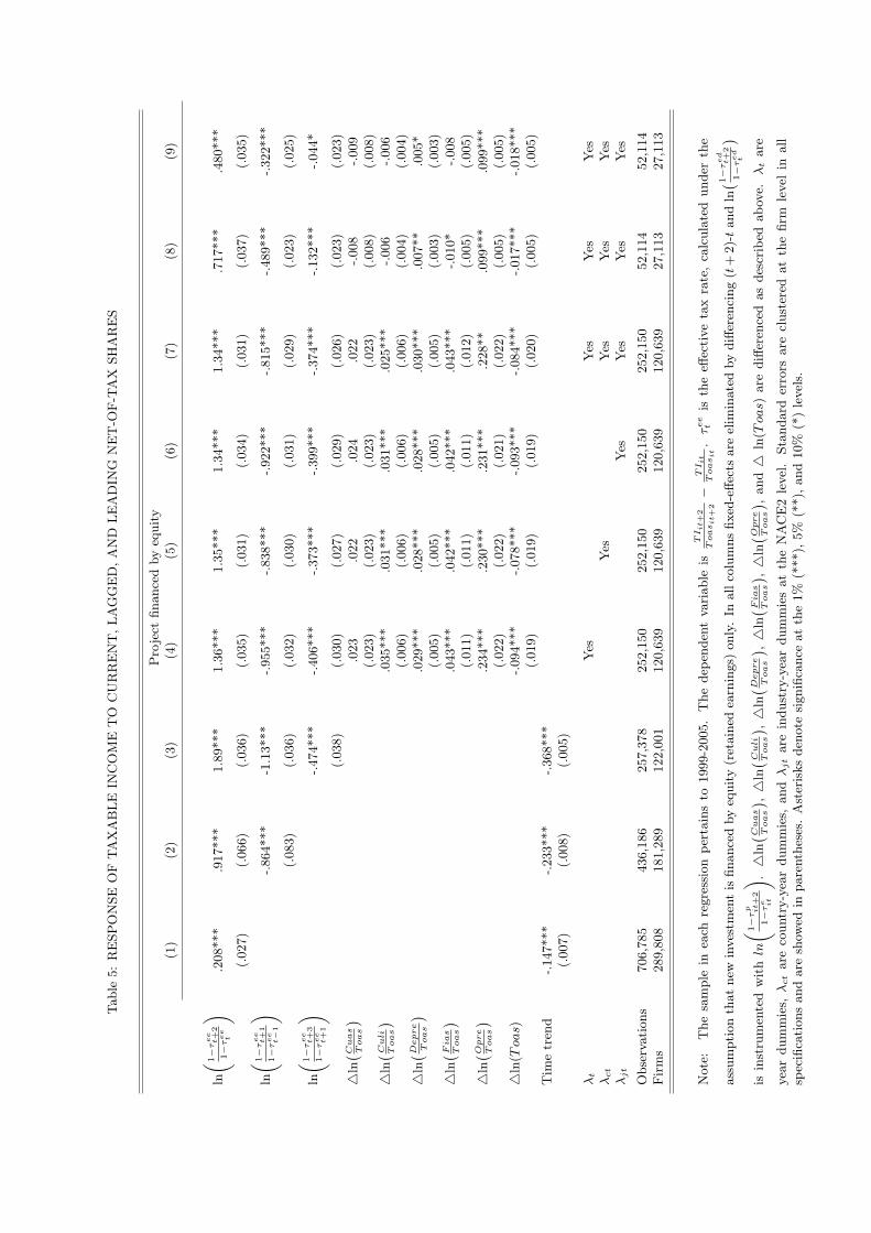
The main results are presented in Table 5. Firm fixed effects are eliminated throughsecond-differencing in all specifications. The effective tax rate is calculated based on arate of return, which does not include interest payments for reasons described above,and the assumption that the project is financed by equity. Column (1) shows the basicregression of the change in the ratio of taxable income to total assets on the change inthe log of the current net-of-tax share, without other controls except a constant, whichacts as a time trend and accounts for income-to-assets growth. The contemporaneouseffect is estimated to be 0.208, and given the specification, it should suffer from omittedvariable bias. If the correlations between the current and lagged and the current andleading net-of-tax shares were positive, then this bias would be downward.

Column (2) allows for a lagged transitory component, which has a negative andstatistically significant impact on the change of taxable income. Note the dramaticincrease in the current tax effect due to mitigation of the omitted variable bias. Thissuggests that while the contemporaneous effect is close to one, part of it is due to atiming shift of income from previous years with higher CIT rates to the current year.

The leading net-of-tax share is added in Column (3) and shows how current TI reactsto anticipated changes in the corporate tax rate. Similarly to the lagged CIT, this termhas a negative impact on reported income, indicating that firms act on expectations oflower taxes in the future by deferring the declaration of income, accelerating expenses,or by other means. Both the current and lagged tax terms grow as a consequence of theinclusion of future taxes.

The current effect in Column (3) is much higher than that of Columns (1) and (2) andis estimated for firms who have at least 5 years of data. As a consequence, compared toColumn (1), the number of firms is more than cut in half in the specification including allthree net-of-tax shares, revealing a major loss of observations due to second-differencing,but also the extent to which the panel is unbalanced. The non-transitory response, orthe sum of the three coefficients, is approximately 0.28 and significant.

The inclusion of the year fixed effects in Column (4), which is equivalent to a diff-in-

25

Tab

le5:

RESP

ONSE

OFTAXABLE

INCOME

TO

CURRENT,L

AGGED,A

ND

LEADIN

GNET-O

F-TAX

SHARES

Project

finan

cedby

equity

(1)

(2)

(3)

(4)

(5)

(6)

(7)

(8)

(9)

ln( 1−τee

t+

2

1−τee

t

).208***

.917***

1.89***

1.36***

1.35***

1.34***

1.34***

.717***

.480***

(.027)

(.066)

(.036)

(.035)

(.031)

(.034)

(.031)

(.037)

(.035)

ln( 1−τee

t+

1

1−τee

t−

1

)-.8

64***

-1.13***

-.955***

-.838***

-.922***

-.815***

-.489***

-.322***

(.083)

(.036)

(.032)

(.030)

(.031)

(.029)

(.023)

(.025)

ln( 1−τee

t+

3

1−τee

t+

1

)-.4

74***

-.406***

-.373***

-.399***

-.374***

-.132***

-.044*

(.038)

(.030)

(.027)

(.029)

(.026)

(.023)

(.023)

4ln( Cua

sToas

).023

.022

.024

.022

-.008

-.009

(.023)

(.023)

(.023)

(.023)

(.008)

(.008)

4ln( Cul

iToas

).035***

.031***

.031***

.025***

-.006

-.006

(.006)

(.006)

(.006)

(.006)

(.004)

(.004)

4ln( Dep

re

Toas

).029***

.028***

.028***

.030***

.007**

.005*

(.005)

(.005)

(.005)

(.005)

(.003)

(.003)

4ln( Fia

sToas

).043***

.042***

.042***

.043***

-.010*

-.008

(.011)

(.011)

(.011)

(.012)

(.005)

(.005)

4ln( Opr

eToas

).234***

.230***

.231***

.228**

.099***

.099***

(.022)

(.022)

(.021)

(.022)

(.005)

(.005)

4ln(Toas)

-.094***

-.078***

-.093***

-.084***

-.017***

-.018***

(.019)

(.019)

(.019)

(.020)

(.005)

(.005)

Tim

etren

d-.1

47***

-.233***

-.368***

(.007)

(.008)

(.005)

λt

Yes

Yes

Yes

Yes

λct

Yes

Yes

Yes

Yes

λjt

Yes

Yes

Yes

Yes

Observation

s706,785

436,186

257,378

252,150

252,150

252,150

252,150

52,114

52,114

Firms

289,808

181,289

122,001

120,639

120,639

120,639

120,639

27,113

27,113

Note:

The

samplein

each

regression

pertains

to1999-2005.

The

depe

ndentvariab

leis

TIit+

2

Toasit+

2−

TIit

Toasit.τeet

istheeff

ective

taxrate,calculated

unde

rthe

assumptionthat

new

investmentisfin

ancedby

equity

(retaine

dearnings)on

ly.In

allc

olum

nsfix

ed-effe

ctsareelim

inated

bydiffe

rencing(t+2)-tan

dln( 1−τ

ed

t+

2

1−τed

t

)is

instrumentedwithln

( 1−τp it+

2

1−τe it

) .4ln( Cua

sToas

) ,4ln( Cul

iToas

) ,4ln( Dep

re

Toas

) ,4ln( Fia

sToas

) ,4ln( Opr

eToas

) ,an

d4

ln(Toas)

arediffe

renced

asde

scribe

dab

ove.

λtare

year

dummies,λctarecoun

try-year

dummies,

andλjtareindu

stry-yeardu

mmiesat

theNACE2level.

Stan

dard

errors

areclusteredat

thefirm

levelin

all

specification

san

dareshow

edin

parenthe

ses.

Asterisks

deno

tesign

ificanceat

the1%

(***),

5%(**),a

nd10%

(*)levels.

diff estimation, means that the response of taxable income is identified using solelythe cross-sectional variation of the net-of-tax shares. Once other firm-level explanatoryvariables and year dummies are controlled for, both the current response and the shiftingcoefficients decrease, resulting in a long-term effect that is statistically not different fromzero.

In particular, Column (4) accounts for the log-change in current assets (cuas), currentliabilities (culi), depreciation (depre), fixed assets (fias), and operating revenue (opre),all scaled by total assets and the change in total assets themselves. An increase in cuas,opre, depre, fias, and culi raises the taxable income-total assets ratio, although thecoefficient of cuas is not precisely estimated. By construction, an increase in Toas willdecrease the TI

Toas ratio. The positive sign of current liabilities seems counter-intuitive,but it may in fact reflect the possibility that highly indebted firms, which are close toviolating debt covenants, may be unwilling to engage in aggressive tax planning. Thisis likely, given that debt covenants not only require the maintenance of certain financialhealth, but also determine how the numbers proving this financial health are calculated.

To purge the regression from country-specific shocks, Column (5) contains country-year fixed effects. In this case the coefficients of interest are identified from the differenttiming and different size of the tax cuts and magnitude of other tax reforms acrosscountries, yielding lower shifting coefficients in absolute value and thus, a positive andsignificant long-run response of .139.

Alternatively, Column (6) controls for shocks such as regulations and industry normsthat affect different sectors differently by incorporating industry-year dummies at theNACE2 level. Similarly to the estimation with year dummies only, controlling forindustry-year fixed effects leads to a permanent response that is not significantly dif-ferent from zero.

Finally, year-, country-year and industry-year fixed effects are all allowed for in Col-umn (7). This extensive dummy structure generates the largest significant non-transitoryeffect, .151, which nevertheless closely resembles the result in Column (5).

Utilising the richest specification, (8) repeats the regression in (7), but this time usingan effective tax rate, which includes interest payments, i.e., the rate of return is comprisedof all elements of added value. The number of firms falls drastically to about 27,000.Although the coefficients of all three net-of-tax shares decrease substantially using thissubsample of firms, income shifting is still present as signalled by the magnitude of thetransitory components, while the long-run effect is almost identical to the one estimatedin Column (7).

The influence of current liabilities is no longer significant, while that of fixed assets

27

becomes negative. In view of the number of tax incentives and deductions available tonew investment in CEE, the negative effect of fias is not unexpected, especially giventhat 66% of the 27,000 firms reporting interest payments are big and medium enterprises.

To check if it is the inclusion of interest payments in the calculation of τ ee that drivesthe lower coefficients in (8) or the particular subsample of firms used, Column (9) reportsresults based on the same subsample, but using the baseline EATR, i.e. ones withoutinte. On account of the results in (9), it can be concluded that the lower estimatedcoefficients are subsample-specific.

5.2 First-difference estimates

Table 7 re-estimates some of the regressions from Table 5 in first-differences. To ob-tain coefficients on the leading and lagged net-of-tax shares, a firm should be present inthe panel for at least four years, whereas a year of data is lost due to first-differencing.Nevertheless, about 54,000 firms that dropped out of the previous estimation as a conse-quence of employing a two-year window are re-incorporated. The trade-off, as explainedin Section 4.4, is the inconsistency of the first stage estimation which spills over to the2SLS coefficients, although, due to not controlling for loss carryforwards, some bias isbound to remain in second-differences as well.

The interesting problem here is that due to the presence of fixed effects and laggedand leading terms of an explanatory variable that is endogenous, the first stage of the2SLS estimation suffers from the classic endogeneity inherent in dynamic panel datamodels. This endogeneity stems from the leading and lagged net-of-tax shares, both ofwhich are exogenous in the original regression but become endogenous in the first stageand hence cannot act as their own instruments as they violate the exclusion restriction.

Even so, it is useful to compare the first-difference estimates to the results in Table 5,bearing in mind that apart from Column (1), the coefficients in Table 7 are inconsistent.The negative correlation of the leading and lagged net-of-tax shares with the error termin the first stage will lead to downward bias in their coefficients, although it is not clearhow it will affect the coefficient of the instrument and thus the fitted value ˆIV .13 Thepredicted error from the first stage, which in general should be orthogonal to the right-hand side of the second-stage regression, contains a bias term. The direction of bias ofthe 2SLS coefficients will therefore depend on the interaction between the conditionalcorrelations and this bias term.14

13See Section 4.4 and the discussion under eq.(6) and (7).14I am thankful to Štěpán Jurajda for this comment.

28

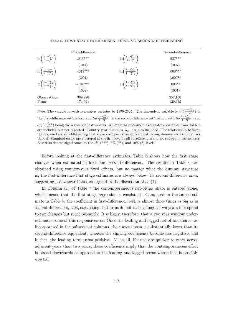
Table 6: FIRST STAGE COMPARISON: FIRST- VS. SECOND-DIFFERENCING

First-difference Second-difference

ln(

1−τpt+1

1−τeet

).813*** ln

(1−τpt+2

1−τeet

).937***

(.014) (.007)

ln(

1−τeet1−τeet−1

)-.019*** ln

(1−τeet+1

1−τeet−1

).008***

(.001) (.0008)

ln(

1−τeet+2

1−τeet+1

)-.046*** ln

(1−τeet+3

1−τeet+1

).003**

(.003) (.001)

Observations 399,286 252,150Firms 174,091 120,639

Note: The sample in each regression pertains to 1999-2005. The dependent variable is ln( 1−τeet+1

1−τeet) in

the first-difference estimation, and ln( 1−τeet+2

1−τeet) in the second-difference estimation, with ln(

1−τpt+1

1−τeet), and

ln(1−τpt+2

1−τeet) being the respective instruments. All other balance-sheet explanatory variables from Table 5

are included but not reported. Country-year dummies, λct, are also included. The relationship betweenthe first-and second-differencing first stage coefficients remains robust to any dummy structure or lackthereof. Standard errors are clustered at the firm level in all specifications and are showed in parentheses.Asterisks denote significance at the 1% (***), 5% (**), and 10% (*) levels.

Before looking at the first-difference estimates, Table 6 shows how the first stagechanges when estimated in first- and second-differences. The results in Table 6 areobtained using country-year fixed effects, but no matter what the dummy structureis, the first-difference first stage estimates are always below the second-difference ones,suggesting a downward bias, as argued in the discussion of eq.(7).

In Column (1) of Table 7 the contemporaneous net-of-tax share is entered alone,which means that the first stage regression is consistent. Compared to the same esti-mate in Table 5, the coefficient in first-difference, .544, is almost three times as big as insecond-differences, .208, suggesting that firms do not take as long as two years to respondto tax changes but react promptly. It is likely, therefore, that a two year window under-estimates some of this responsiveness. Once the leading and lagged net-of-tax shares areincorporated in the subsequent columns, the current term is substantially lower than itssecond-difference equivalent, whereas the shifting coefficients become less negative, andin fact, the leading term turns positive. All in all, if firms are quicker to react acrossadjacent years than two years, these coefficients imply that the contemporaneous effectis biased downwards as opposed to the leading and lagged terms whose bias is possiblyupward.

29

Table 7: RESPONSE OF TAXABLE INCOME TO CURRENT, LAGGED, AND LEADING NET-OF-TAX SHARES, FIRST-DIFFERENCE ESTIMATION

(1) (2) (3) (4) (5)

ln(

1−τeet+1

1−τedt

).544*** 1.33*** 1.20*** 1.22*** 1.25***

(.049) (.099) (.053) (.052) (.053)

ln(

1−τeet1−τeet−1

)-.845*** -.618*** -.634*** -.603***

(.040) (.034) (.034) (.033)

ln(

1−τeet+2

1−τeet+1

).615*** .253*** .144*** .231***

(.047) (.021) (.020) (.020)

λt Yesλct Yesλjt Yes

Observations 1,071,593 408,278 399,286 399,286 399,286Firms 417,938 177,009 174,091 174,091 174,091

Note: The sample in each regression pertains to 1999-2005. The dependent variable is TIit+1

Toasit+1− TIit

Toasit.

τeet is the effective tax rate, calculated under the assumption that new investment is financed by equity(retained earnings) only. In all columns fixed-effects are eliminated by first-differencing (t + 1)-t, and

ln( 1−τeet+1

1−τeet

)is instrumented with ln

( 1−τpt+1

1−τeet

). All other balance-sheet explanatory variables from Table

5 are included in Columns (3)-(5) in first-differences and not reported here. λt are year dummies, λctare country-year dummies, and λjt are industry-year dummies at the NACE2 level. Standard errorsare clustered at the firm level in all specifications and are showed in parentheses. Asterisks denotesignificance at the 1% (***), 5% (**), and 10% (*) levels.

5.3 Who shifts income?

This section investigates in more detail what type of firms drive the non-transitory re-sult, and in particular, whether the effect varies by firm size and ability to shift income.Large firms especially may be more sensitive to nontax costs of income deferral, but mayalso be more effective at shifting income as they have more sophisticated tax depart-ments. Guenther (1994) and Scholes et al. (1992) describe two types of nontax costs: (1)those associated with income deferral such as costs caused by the acceleration of R&Dprojects or dissatisfied customers if year-end shipments are delayed, and (2) politicalcosts pertaining to meeting debt covenant restrictions and management compensationplans. Guenther (1994) concludes that larger firms will tend to reduce financial state-ment income if they defer taxable income to minimise cost in case they are subjectedto public scrutiny. Scholes et al. (1992) estimates that large public firms are more taxopportunistic than small public companies and are more prone to shifting gross marginand selling, general and administrative expenses in expectation of tax cuts.

30

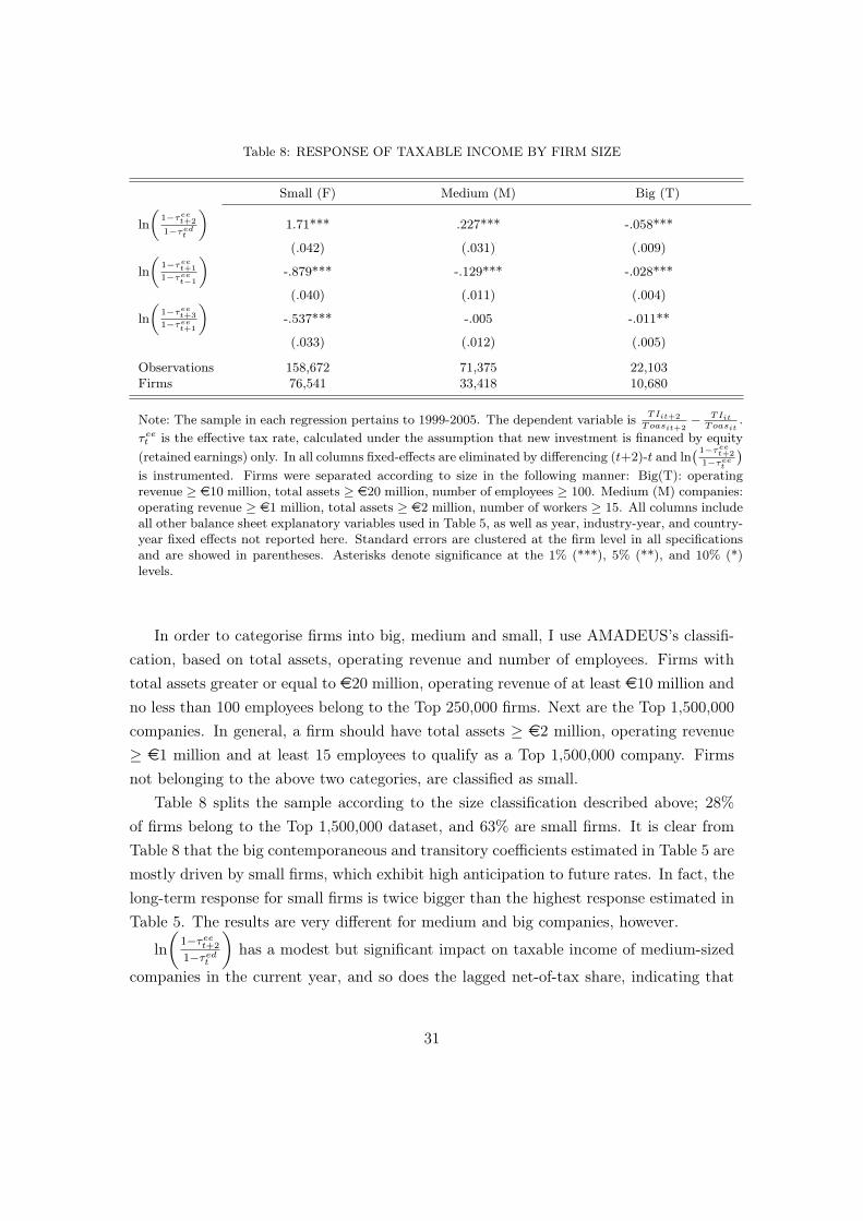
Table 8: RESPONSE OF TAXABLE INCOME BY FIRM SIZE

Small (F) Medium (M) Big (T)

ln(

1−τeet+2

1−τedt

)1.71*** .227*** -.058***

(.042) (.031) (.009)

ln(

1−τeet+1

1−τeet−1

)-.879*** -.129*** -.028***

(.040) (.011) (.004)

ln(

1−τeet+3

1−τeet+1

)-.537*** -.005 -.011**

(.033) (.012) (.005)

Observations 158,672 71,375 22,103Firms 76,541 33,418 10,680

Note: The sample in each regression pertains to 1999-2005. The dependent variable is TIit+2

Toasit+2− TIit

Toasit.

τeet is the effective tax rate, calculated under the assumption that new investment is financed by equity(retained earnings) only. In all columns fixed-effects are eliminated by differencing (t+2)-t and ln

( 1−τeet+2

1−τeet

)is instrumented. Firms were separated according to size in the following manner: Big(T): operatingrevenue ≥ e10 million, total assets ≥ e20 million, number of employees ≥ 100. Medium (M) companies:operating revenue ≥ e1 million, total assets ≥ e2 million, number of workers ≥ 15. All columns includeall other balance sheet explanatory variables used in Table 5, as well as year, industry-year, and country-year fixed effects not reported here. Standard errors are clustered at the firm level in all specificationsand are showed in parentheses. Asterisks denote significance at the 1% (***), 5% (**), and 10% (*)levels.

In order to categorise firms into big, medium and small, I use AMADEUS’s classifi-cation, based on total assets, operating revenue and number of employees. Firms withtotal assets greater or equal to e20 million, operating revenue of at least e10 million andno less than 100 employees belong to the Top 250,000 firms. Next are the Top 1,500,000companies. In general, a firm should have total assets ≥ e2 million, operating revenue≥ e1 million and at least 15 employees to qualify as a Top 1,500,000 company. Firmsnot belonging to the above two categories, are classified as small.

Table 8 splits the sample according to the size classification described above; 28%of firms belong to the Top 1,500,000 dataset, and 63% are small firms. It is clear fromTable 8 that the big contemporaneous and transitory coefficients estimated in Table 5 aremostly driven by small firms, which exhibit high anticipation to future rates. In fact, thelong-term response for small firms is twice bigger than the highest response estimated inTable 5. The results are very different for medium and big companies, however.

ln(

1−τeet+2

1−τedt

)has a modest but significant impact on taxable income of medium-sized

companies in the current year, and so does the lagged net-of-tax share, indicating that

31

medium-sized firms undertake income shifting on a small scale. The leading effect, whilenegative, is insignificant. After accounting for income shifting, the non-transitory effecton TI for medium firms is much closer to the one obtained with the full sample.

When it comes to big firms, the current net-of-tax share has a negative and significanteffect on taxable income, a contradictory result to the previous estimates. While both thelagged and leading change in tax rates have precisely estimated negative impact on TI,these effects are rather small. Big firms, therefore, do not seem to engage in aggressiveintertemporal earnings management.

Considering bigger firms’ access to many other tax management instruments, such asdebt shifting, earnings distribution between subsidiaries, geographic income shifting, aswell as investment tax incentives, it is probable that such firms find cheaper alternativesto the intertemporal shifting of income (Tang and Jog, 2001; Smart and Hong, 2010).This result is robust to splitting the sample by firms’ number of managers, which can beused as a proxy for firm size.15

Another sample split, this time by country, is performed in Table 9 with the resultsvarying greatly between countries. First, Bulgaria and Slovakia have negative estimatedcoefficients for the current effect, which are also statistically significant. An insignificantnegative contemporaneous term is estimated for Hungary. Given that 75% of the totalsample are Romanian firms, the coefficients for this county are closest to the full sampleones, as expected. Last but not least, Poland exhibits a modest current effect and smalltransitory coefficients, while in the case of the Czech Republic these effects are bigger,yet still well below the full sample estimates.

In a sense, however, Table 9 replicates the sample splits from Table 8, since 47,254out of the 55,642 firm-year observations, or 84%, for Bulgaria, the Czech Republic, Hun-gary, Poland and Slovakia are medium and big enterprises, for whom small positive andnegative current net-of-tax share coefficients are estimated, respectively. It is, therefore,hard to consider the samples for these five countries representative, as most of the smallerfirms simply do not appear in the panel for five consecutive years and drop out of theestimation. In the other extreme is Romania, with 74% small and 23% medium firms.

15In general I would expect that a firm’s ability to shift income will increase proportionally to thenumber of managers it employs. Yet, this turns out not to be the case. The sample is divided intothree subgroups: firms with zero to two managers, those with 2 up to 5 managers and firms employingmore than 5 managers. The results are robust to using other subgroups and are almost identical tothose in Table 8, with the most responsive firms being the ones with fewer managers, whereas companieswith five or more managers have very small shifting coefficients. One possible explanation put forthby Guenther (1994) is that if management compensation is linked to firm performance, then executivesmay be reluctant to decrease taxable income to save taxes, even though this move would be beneficial toshareholders. Alternatively, as mentioned earlier, big firms can utilise a variety of tax instruments apartfrom income shifting, which are not easily procurable by smaller companies.

32

Table 9: RESPONSE OF TAXABLE INCOME BY COUNTRY

BG CZ HU PL RO SK

ln(

1−τeet+2

1−τeet

)-.249*** .467*** -.988 .169*** 1.66*** -.108***

(.009) (.096) (.641) (.014) (.035) (.047)

ln(

1−τeet+1

1−τeet−1

)-.020** -.295** -.236 -.043*** -.928*** -.022

(.006) (.135) (.144) (.009) (.033) (.017)

ln(

1−τeet+3

1−τeet+1

)-.011*** -.287*** .386 -.005 -.417** .002

(.003) (.075) (.508) (.006) (.028) (.024)

Observations 15,712 10,212 13,783 13,929 196,508 2,006Firms 7,326 6,460 7,012 7,273 91,440 1,128

Note: The sample in each regression pertains to 1999-2005. The dependent variable is TIit+2

Toasit+2− TIit

Toasit.

τeet is the effective tax rate, calculated under the assumption that new investment is financed by equity(retained earnings) only. In all columns fixed-effects are eliminated by differencing (t+2)-t and ln

( 1−τeet+2

1−τeet

)is instrumented. The sample is split by country. All columns include all other balance sheet explanatoryvariables used in Table 5, as well as year and industry-year effects, not reported here. Standard errorsare clustered at the firm level in all specifications and are showed in parentheses. Asterisks denotesignificance at the 1% (***), 5% (**), and 10% (*) levels.

As a robustness check, Table 10 repeats the regressions from Table 5, using theeffective tax rate τ ed, based on the assumption that the project is entirely financedby debt. The current effect is twice as high as the one estimated with τ ee, but fallssubstantially when the lagged tax rates are added. Without controlling for any otherfirm-level variables, Column (3) actually yields a negative and significant non-transitoryresponse. Once other explanatory variables and year dummies are accounted for inColumn (4), the long-run effect is 0.258, which is higher than the one obtained with thesame specification using τ ee. The richest specification in Column (7), however, producesa non-transitory effect of 0.031, which is not significantly different from zero. Similarly tothe regressions with τ ee, the estimates with τ ed lead to a long-run response that is eitherclose to zero, or small, positive and significant, depending on the dummy structure.

In general, assuming a project financed by debt results in lower estimated coefficientsof the net-of-tax shares in absolute value than a project financed by equity. This may bedue to the fact that, unlike financing with equity (retained earnings), the cost of raisingexternal capital through debt, F , is different from zero, which in turn yields higher net-present value R and hence smaller τ ed. Compared to τ ee, the distribution of τ ed is thusshifted to the left, as shown in Figures 4 and 5. With more values of τ ed closer to zero,it is not surprising that a flatter line is estimated with this tax rate than with τ ee.

33

Tab

le10:RESP

ONSE

OFTAXABLE

INCOME

TO

CURRENT,L

AGGED,A

ND

LEADIN

GNET-O

F-TAX

SHARES

Project

finan

cedby

debt

(1)

(2)

(3)

(4)

(5)

(6)

(7)

(8)

ln( 1−τed

t+

2

1−τed

t

).479***

.102*

.808***

1.07***

.665***

1.10***

.696***

.296***

(.047)

(.056)

(.061)

(.077)

(.079)

(.074)

(.076)

(.066)

ln( 1−τed

t+

1

1−τed

t−

1

)-.4

97***

-.787***

-.549***

-.472***

-.529***

-.459***

-.314***

(.040)

(.028)

(.040)

(.026)

(.027)

(.026)

(.044)

ln( 1−τed

t+

3

1−τed

t+

1

)-.4

68***

-.263***

-.199***

-.262***

-.206***

-.076**

(.038)

(.033)

(.026)

(.032)

(.026)

(.034)

4ln( Cua

sToas

).028

.027

.028

.027

-.006

(.037)

(.037)

(.036)

(.037)

(.010)

4ln( Cul

iToas

).071***

.065***

.065***

.058***

-.001

(.012)

(.012)

(.012)

(.012)

(.006)

4ln( Dep

re

Toas

).003

.0009

.002

.0009

-.001

(.014)

(.015)

(.014)

(.014)

(.003)

4ln( Fia

sToas

).005

.011

.006

.013

-.030***

(.017)

(.017)

(.017)

(.017)

(.007)

4ln( Opr

eToas

).328***

.326***

.326***

.323***

.107***

(.054)

(.054)

(.054)

(.054)

(.007)

4ln(Toas)

-.102***

-.100***

-.101***

-.100***

-.027***

(.020)

(.021)

(.020)

(.022)

(.006)

Tim

etren

d-.0

86***

-.252***

-.407***

(.007)

(.011)

(.004)

λt

Yes

Yes

Yes

λct

Yes

Yes

Yes

λjt

Yes

Yes

Yes

Observation

s671,257

410,098

243,473

238,549

238,549

238,549

238,549

51,085

Firms

280,633

175,090

118,509

117,112

117,112

117,112

117,112

26,645

Note:

The

samplein

each

regression

pertains

to1999-2005.

The

depe

ndentvariab

leis

TIit+

2

Toasit+

2−

TIit

Toasit.τedt

istheeff

ective

taxrate,c

alculatedun

der

theassumptionthat

new

investmentis

finan

cedby

debt

only.In

allcolumns

fixed

-effe

ctsareelim

inated

bydiffe

rencing(t

+2)-tan

dln(1−τed

t+

2

1−τed

t)is

instrumented.4ln( Cua

sToas

) ,4ln( Cul

iToas

) ,4ln( Dep

re

Toas

) ,4ln( Fia

sToas

) ,4ln( Opr

eToas

) ,and4

ln(Toas)

arediffe

renced

asde

scribe

dab

ove.λtareyear

dummies,

λctarecoun

try-year

dummies,an

dλjtareindu

stry-yeardu

mmiesat

theNACE2level.Stan

dard

errors

areclusteredat

thefirm

levelinallspe

cifications

andareshow

edin

parenthe

ses.

Asterisks

deno

tesign

ificanceat

the1%

(***),5%

(**),a

nd10%

(*)levels.

6 Conclusion

In the last two decades most CEE countries undertook radical tax cuts as part of apackage of tax reforms speeding up their transition from controlled to competitive marketeconomies. The considerable decline in the CIT rates contributed to a reduction in illiciteconomic activities, encouraged new entrepreneurs and stimulated already existing firmsto expand, thus leading to a remarkable stability of revenue collections.

This paper explores whether firms resort to income shifting across years in antici-pation of lower tax rates as an additional mechanism that can explain the increase ofcorporate revenue in the years taxes were cut. A substantial rise in revenue in a taxcut year occurs at the expense of previous year collections if income shifting is present.Further, if tax declines are expected in the future, taxable income can be shifted further.

The shifting of income, however, is simply a timing response that does not distort realeconomic behaviour, and, if unaccounted for, would wrongfully inflate the deadweightloss of the CIT. Thus, the estimates of the current effect of the net-of-tax shares yieldlarge coefficients, implying a 0.01 increase in the difference of the taxable income-totalassets ratio as a result of a 1% increase in the two year difference between the net-of-tax rates. Given an average TI

Toas ratio of 0.08, a 0.01 increase is substantial. Whenthe possibility of income shifting is explicitly modelled by the inclusion of leading andlagged terms, the sum of the three coefficients is in the range between zero and .15 (.20 ifτ ed estimates are considered). Nevertheless, even the positive estimated non-transitoryresponses have a negligible effect on TI

Toas as compared to the current response only.The results suggest that small firms are most responsive to anticipated tax cuts, ex-

hibiting the largest shifting coefficients as well as the largest long-term response, followedby medium enterprises. In contrast, the estimated current effect for big firms is negative,leading to negative and significant permanent responses. This finding is to some extentmimicked by country sample splits, since the subsamples for five of the CEE countries,Romania being excluded, are composed largely of medium and Top 250,000 firms, mainlydue to the requirement that a firm appears in the panel for at least five years. For thisreason, outside of the sample results, it cannot be conclusively stated that the estimatesfor the Czech Republic and Poland are smaller than for Romania because firms there areless responsive to tax changes, or that firms in Bulgaria, Hungary, and Slovakia behavedifferently given the negatively estimated current effects.

35

References

Bond, S., 2002. Dynamic panel data models: A guide to micro data methods and practice.Working Paper CWP09/02, CEMMAP, London,UK.

Cameron, A. C., Trivedi, P. K., 2009a. Microeconometrics. Methods and Applications.Cambridge University Press, New York, NY.

Cameron, A. C., Trivedi, P. K., 2009b. Microeconometrics Using Stata. Stata Press,College Station, TX.

Clausing, K. A., 2007. Corporate tax revenues in OECD countries. International Tax andPublic Finance 14 (2), 115–133.

Da Rin, M., Di Giacomo, M., Sembenelli, A., 2011. Entrepreneurship, firm entry, andthe taxation of corporate income: Evidence from Europe. Journal of Public Economics95 (9-10), 1048–1066.

Devereux, M. P., Griffith, R., 2003. Evaluating tax policy for location decisions. Interna-tional Tax and Public Finance 10 (2), 107–126.

Devereux, M. P., Griffith, R., Klemm, A., 2004. Why has the UK corporation tax raisedso much revenue? Fiscal Studies 25 (4), 367–388.

Dwenger, N., Steiner, V., 2012. Profit taxation and the elasticity of the corporate incometax base: Evidence from German corporate tax return data. National Tax Journal,forthcoming.

Ernst & Young, Various years. Worldwide corporate tax guide. Ernst & Young.

European Commission, 2010. Green paper on the future of VAT. Towards a simpler, morerobust and efficient VAT system. COM(2010)695 SEC(2010)1455, Brussels.

European Commission, Various years. Taxation trends in the European Union. Data forthe EU member states, Iceland and Norway. Publications office of the European Union,Luxembourg.

Goolsbee, A., 2000. What happens when you tax the rich? Evidence from executivecompensation. Journal of Political Economy 108 (2), 352–378.

Gruber, J., Rauh, J., 2007. How elastic is the corporate income tax base? In: Auer-bach, A., Hines, J., Slemrod, J. (Eds.), Taxing Corporate Income in the 21st Century.Cambridge University Press, Cambridge, UK, pp. 140–163.

36

Guenther, D. A., 1994. Earnings management in response to corporate tax rate changes:Evidence from the 1986 Tax Reform Act. The Accounting Review 69 (1), 230–243.

Hanlon, M., 2003. What can we infer about a firm’s taxable income from its financialstatements? National Tax Journal 56 (4), 831–863.

Heim, B. T., 2006. The elasticity of taxable income: Evidence from a new panel of taxreturns. Office of Tax Analysis Working Paper, Washington, DC.

Kalwij, A. S., 2003. A maximum likelihood estimator based on first differences for paneldata Tobit model with individual specific effects. Economic Letters 81 (6), 165–172.

King, M. A., 1974. Taxation and the cost of capital. The Review of Economic Studies41 (1), 21–35.

Klapper, L., Laeven, L., Rajan, R., 2006. Entry regulation as a barrier to entrepreneur-ship. Journal of Financial Economics 82 (3), 591–629.

KPMG Poland, 2009. A guide to special economic zones in Poland. KPMG.

Mintz, J. M., 1988. An empirical estimate of corporate tax refundability and effectivetax rates. Quarterly Journal of Economics 103 (1), 225–231.

Nickell, S., 1981. Biases in dynamic models with fixed effects. Econometrica 49 (6), 1417–1426.

Piotrowska, J., Vanborren, W., 2008. The corporate income tax rate-revenue paradox:Evidence in the EU. Working Paper 12, Brussels.

Roubi, R. R., Richardson, A. W., 1998. Managing discretionary accruals in response toreductions in corporate tax rates in Canada, Malaysia and Singapore. The InternationalJournal of Accounting 33 (4), 455–467.

Scholes, M. S., Wilson, G. P., Wolfson, M. A., 1992. Firms’ responses to anticipatedreductions in tax rates: The Tax Reform Act of 1986. Journal of Accounting Research30, 161–185.

Slemrod, J., 1995. Income creation or income shifting? Behavioral responses to the TaxReform Act of 1986 . A.E.A. Papers and Proceedings 85 (2), 175–180.

Smart, M., Hong, Q., 2010. In praise of tax havens: International tax planning andforeign direct investment. European Economic Review 54 (1), 82–95.

37

Tang, J., Jog, V. M., 2001. Tax reforms, debt shifting and tax revenues: Multinationalcorporations in Canada. International Tax and Public Finance 8 (1), 5–25.

United Nations, 2000. Tax incentives and foreign direct investment: A global survey.ASIT Advisory Studies No. 16, Geneva.

38

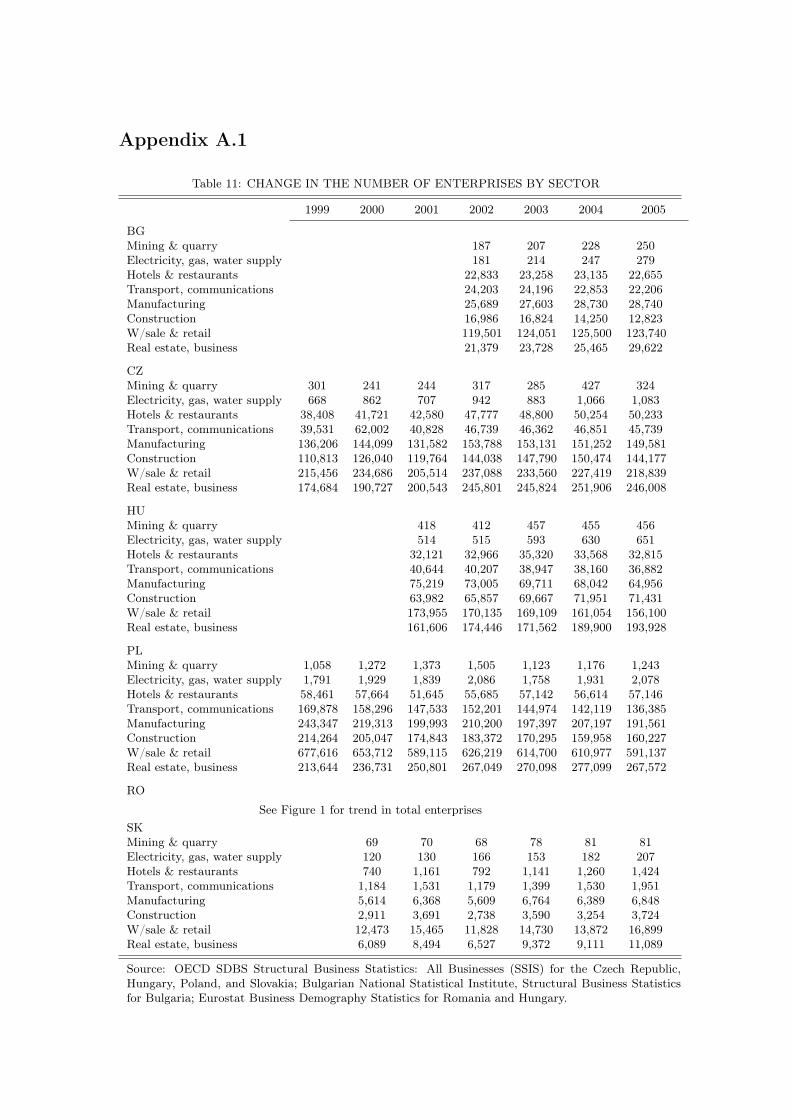
Appendix A.1

Table 11: CHANGE IN THE NUMBER OF ENTERPRISES BY SECTOR

1999 2000 2001 2002 2003 2004 2005

BGMining & quarry 187 207 228 250Electricity, gas, water supply 181 214 247 279Hotels & restaurants 22,833 23,258 23,135 22,655Transport, communications 24,203 24,196 22,853 22,206Manufacturing 25,689 27,603 28,730 28,740Construction 16,986 16,824 14,250 12,823W/sale & retail 119,501 124,051 125,500 123,740Real estate, business 21,379 23,728 25,465 29,622

CZMining & quarry 301 241 244 317 285 427 324Electricity, gas, water supply 668 862 707 942 883 1,066 1,083Hotels & restaurants 38,408 41,721 42,580 47,777 48,800 50,254 50,233Transport, communications 39,531 62,002 40,828 46,739 46,362 46,851 45,739Manufacturing 136,206 144,099 131,582 153,788 153,131 151,252 149,581Construction 110,813 126,040 119,764 144,038 147,790 150,474 144,177W/sale & retail 215,456 234,686 205,514 237,088 233,560 227,419 218,839Real estate, business 174,684 190,727 200,543 245,801 245,824 251,906 246,008

HUMining & quarry 418 412 457 455 456Electricity, gas, water supply 514 515 593 630 651Hotels & restaurants 32,121 32,966 35,320 33,568 32,815Transport, communications 40,644 40,207 38,947 38,160 36,882Manufacturing 75,219 73,005 69,711 68,042 64,956Construction 63,982 65,857 69,667 71,951 71,431W/sale & retail 173,955 170,135 169,109 161,054 156,100Real estate, business 161,606 174,446 171,562 189,900 193,928

PLMining & quarry 1,058 1,272 1,373 1,505 1,123 1,176 1,243Electricity, gas, water supply 1,791 1,929 1,839 2,086 1,758 1,931 2,078Hotels & restaurants 58,461 57,664 51,645 55,685 57,142 56,614 57,146Transport, communications 169,878 158,296 147,533 152,201 144,974 142,119 136,385Manufacturing 243,347 219,313 199,993 210,200 197,397 207,197 191,561Construction 214,264 205,047 174,843 183,372 170,295 159,958 160,227W/sale & retail 677,616 653,712 589,115 626,219 614,700 610,977 591,137Real estate, business 213,644 236,731 250,801 267,049 270,098 277,099 267,572

RO

See Figure 1 for trend in total enterprisesSKMining & quarry 69 70 68 78 81 81Electricity, gas, water supply 120 130 166 153 182 207Hotels & restaurants 740 1,161 792 1,141 1,260 1,424Transport, communications 1,184 1,531 1,179 1,399 1,530 1,951Manufacturing 5,614 6,368 5,609 6,764 6,389 6,848Construction 2,911 3,691 2,738 3,590 3,254 3,724W/sale & retail 12,473 15,465 11,828 14,730 13,872 16,899Real estate, business 6,089 8,494 6,527 9,372 9,111 11,089

Source: OECD SDBS Structural Business Statistics: All Businesses (SSIS) for the Czech Republic,Hungary, Poland, and Slovakia; Bulgarian National Statistical Institute, Structural Business Statisticsfor Bulgaria; Eurostat Business Demography Statistics for Romania and Hungary.

Table 12: CHANGE IN PROFITABILITY BY SECTOR

1999 2000 2001 2002 2003 2004 2005

BGMining & quarry 0.383 0.163 -0.222 -0.323 0.034 0.169 0.288Electricity, gas, water supply 0.400 0.523 0.402 0.314 0.201 0.235 0.137Hotels & restaurants 0.575 0.548 0.504 0.457 0.407 0.453 0.388Transport, communications 0.347 0.554 0.450 0.465 0.476 0.480 0.431Manufacturing 0.167 0.283 0.300 0.280 0.283 0.281 0.286Construction 0.501 0.520 0.508 0.484 0.446 0.509 0.517W/sale & retail 0.495 0.474 0.472 0.414 0.270 0.303 0.356Real estate, business 0.817 0.805 0.780 0.779 0.76 0.745 0.722

CZMining & quarry 0.372 0.212 0.232 0.209 0.194 0.326 0.393Electricity, gas, water supply 0.136 -0.024 0.102 0.149 0.207 0.281 0.327Hotels & restaurants 0.487 0.426 0.379 0.361 0.420 0.448 0.392Transport, communications 0.273 0.256 0.288 0.325 0.336 0.303 0.270Manufacturing 0.342 0.345 0.325 0.230 0.287 0.342 0.331Construction 0.408 0.402 0.417 0.407 0.421 0.440 0.429W/sale & retail 0.440 0.478 0.464 0.479 0.445 0.380 0.439Real estate, business 0.414 0.431 0.426 0.404 0.388 0.377 0.399

HUMining & quarry -0.271 -0.220 -0.349 -0.104 -0.068 -0.030 0.034Electricity, gas, water supply 0.205 0.155 0.104 0.111 0.120 0.188 0.137Hotels & restaurants 0.361 0.278 0.246 0.280 0.200 0.182 0.160Transport, communications 0.069 0.034 0.053 0.113 0.125 0.147 0.128Manufacturing 0.311 0.287 0.288 0.303 0.326 0.351 0.346Construction 0.449 0.464 0.461 0.481 0.418 0.417 0.371W/sale & retail 0.335 0.271 0.355 0.373 0.312 0.292 0.276Real estate, business 0.478 0.474 0.479 0.487 0.459 0.443 0.425

PLMining & quarry -0.187 -0.008 -0.038 -0.075 -0.045 0.201 0.225Electricity, gas, water supply -0.266 -0.296 -0.176 -0.082 -0.005 -0.015 -0.014Hotels & restaurants 0.424 0.419 0.396 0.457 0.458 0.441 0.457Transport, communications 0.165 0.200 0.241 0.296 0.303 0.334 0.350Manufacturing 0.169 0.191 0.160 0.188 0.260 0.340 0.328Construction 0.518 0.531 0.475 0.505 0.552 0.554 0.574W/sale & retail 0.695 0.700 0.675 0.681 0.651 0.683 0.676Real estate, business 0.615 0.620 0.595 0.608 0.619 0.613 0.627

ROMining & quarry 0.304 0.357 0.161 0.184 0.209 0.191 0.143Electricity, gas, water supply 0.505 0.449 0.275 0.471 0.510 0.496 0.442Hotels & restaurants 0.854 0.747 0.502 0.576 0.592 0.578 0.605Transport, communications 0.725 0.564 0.550 0.581 0.620 0.654 0.626Manufacturing 0.517 0.489 0.439 0.479 0.477 0.505 0.478Construction 0.574 0.541 0.422 0.477 0.574 0.569 0.582W/sale & retail 0.664 0.529 0.505 0.507 0.574 0.588 0.592Real estate, business 0.869 0.869 0.802 0.828 0.849 0.825 0.828

SKMining & quarry 0.205 0.318 0.274 0.125 0.219 0.177 0.224Electricity, gas, water supply 0.103 -0.290 -1.03 -0.542 -0.059 0.127 0.021Hotels & restaurants 0.451 0.442 0.425 0.385 0.416 0.445 0.462Transport, communications 0.417 0.415 0.475 0.398 0.375 0.368 0.350Manufacturing 0.321 0.347 0.37 0.315 0.329 0.393 0.394Construction 0.457 0.607 0.575 0.645 0.559 0.568 0.601W/sale & retail 0.493 0.355 0.469 0.394 0.508 0.553 0.529Real estate, business 0.455 0.458 0.458 0.485 0.440 0.454 0.407

Profitability is measured as corporate net operating surplus divided by corporate value added. SourceEurostat.

Appendix A.2: Identifying firms eligible for tax incentives

The Ernst & Young Worldwide corporate tax guides provide a comprehensive list of thetax incentives introduced over the period 1999-2005. Due to the nature of the qualifyingconditions and data availability, only a subset of these incentives are accounted for, whichare summarised in Table 2. For convenience, I repeat the reforms and eligibility criteriabelow and explain how I have identified firms in the AMADEUS dataset that are eligibleor have used a tax break. The main assumption is that if a firm met the conditions fora tax incentive, it took advantage of it. Nevertheless, this assumption is always doublechecked by looking at what happens to eligible firms’ tax payments.

BulgariaProduction companies qualify for a 100% reduction of the corporate tax on income

for five consecutive years if the following conditions are met: a) The company and itsassets are located in municipalities with unemployment rate for the preceding year 50%higher than the average unemployment rate for the country; b) the tax is accounted foras a reserve and (part of it) is used for the acquisition of long-term fixed assets; c) 80%of workers reside in the above-mentioned municipalities; d) the company does not haveoutstanding liabilities for tax and social insurance contributions. The tax incentive wasintroduced at the beginning of 2003 and is still in force.

A list of the municipalities that satisfy the unemployment rate condition is publishedevery year as an annex of the Bulgarian Corporate Income Tax Law. I matched thecities in which manufacturing companies operate to these municipalities as a first step toidentifying firms eligible for the tax incentive. I then chose only firms whose fixed assetsgrew compared to the previous year. Unfortunately, I cannot account for conditions c)and d), but given that a firm satisfies a) and b), and has reported zero (negative) taxand positive accounting profit, I assume that it took advantage of the tax opportunity.Thus, if a firm qualifies in 2003, its effective tax rate is zero for the remaining yearsit appears in the panel. Approximately 60 firms (254 firm-year observations) meet theabove conditions. Since their taxable income cannot be imputed, earnings before interestand tax are used instead (ebit).

The Czech RepublicInvestors in manufacturing can apply for corporate income tax holiday for up to 10

years subject to conditions which change annually. For a detailed account of these re-quirements, see Ernst & Young (Various years). A list of the qualifying firms for theperiod 1999-2005 is published at http://www.czechinvest.org/en/investment-incentives-for-manufacturing-industry. As the AMADEUS dataset includes the names of the com-

41

panies, it is straightforward to identify the Czech and Czech-based foreign firms that havebeen granted the tax holiday. This tax incentive is in force for the whole time periodconsidered in the paper.

From the Czechinvest list, 167 firms altogether appear in the AMADEUS dataset, orequivalently 781 firm-year observations. Out of these, 426 firm-year observations face azero statutory tax rate. This is because some firms appear in the data a few years beforethey qualified for the tax holiday. Similarly to Bulgarian firms, ebit is used as a measureof these firms’ TI for the relevant years. In 1999 and 2000, only firms belonging to the Top250,000 firms took advantage of the tax holiday. From 2002 onwards, smaller companiesalso joined in utilising the incentive. All of them are part of Dataset M (Top 1.5 millionfirms). AMADEUS’s criteria for Top 250,000 and Top 1.5m firms are described underTable 8 and in the main text.

Over 20% of all firms granted the tax holiday specialise in the manufacture of partsand accessories for motor vehicles and their engines (NACE4 3430) and the manufactureof electrical equipment for engines and vehicles (NACE4 3161).

HungaryHungary offers an investment tax credit of 50% of the corporate tax for two sectors:

manufacturing and the hotel industry. To qualify for the credit, a manufacturing firmshould make an investment of HUF 1 billion ($3.33 million). The credit can be claimedin each of the next consecutive five years if sales revenue increases by an annual averageof 5% of the investment value (Ernst & Young, Various years). Given the conditions, Iidentify manufacturing firms (52 firms, 167 firm-year observations), whose fixed assetsgrew by at least the minimum amount required and assigned 50% lower statutory taxrate for the subsequent years these firms show in the panel, provided that their salesincreased by at least 5% of the minimum investment required.

With respect to hotels, the same amount of investment is necessary – HUF 1 billion.However, in order to claim the credit in the next 5 years, sales should grow by 25%compared to previous year sales but not less than HUF 600 million. Approximately 5-6hotels meet the investment requirement per year in the AMADEUS database, but noneof them meets the sales growth requirement.

PolandPoland has fourteen special economic zones, namely Kamienna Góra, Katowice,

Kostrzyn-Słubice, Kraków, Legnica, Łódź, Mielec, Pomeranian, Słupsk, Starachowice,Suwałki, Tarnobrzeg, Wałbrzych, and Warmia-Mazury. They are described in detail inKPMG Poland (2009). I obtained a list of the investors for each zone from the zone’srespective website and matched it to the data.

42

The AMADEUS dataset contains 272 companies (717 firm-year observations) witha license to operate in one or more of the above zones. Together, these firms employapproximately 110,000 people and have $38 million of total assets, on average. Giventhe investment a company makes, it qualifies for a tax exemption based on the followingformula: I = R(e50 million +0.5B+ 0.34C), where R is the aid intensity in a given eco-nomic zone, B is the amount of investment above e50 million (B ≤ e50million), whileC is the amount of investment exceeding e100 million. Thus, a firm investing e120 mil-lion in Slaskie voivodship is eligible for I = 40%(e50 million +0.5e50 million+0.34e20million)=e32.7 million exemption and the firm will not pay corporate tax until this ex-emption has been exhausted (KPMG Poland, 2009). I use ebit as a measure of whatthese companies’ TI is, even in the years they pay some tax because information on theamount of the credits is unavailable.

RomaniaFrom 2000 to 2004 inclusive, Romania provided incentives for small and medium

enterprises. SMEs CIT was reduced by 20% if their number of employees increased by10% as compared to the preceding year. A SME is defined as a firm that has an annualturnover of less than e8 million and employs no more than 250 employees. Anothercondition is that the capital of a SME is 100% privately owned. I isolated firms meetingthe employment, turnover and ownership conditions and lowered their statutory tax ratesby 20% if their number of employees grew with the required percent. Tax incentives forSMEs were still available in 2005 but depended on profits reinvested in equipment, andtherefore, I am not able to account for them.

About 9,000 firms (42,909 firm-year observations) per year qualified for this incentive,with turnover of $1 million and 38 employees, on average. Close to 40% of the eligiblecompanies were from the retail and wholesale industry. A statutory tax rate of 20% isassigned on a year-to-year basis to the SMEs, which fulfilled the incentive criteria.

Romania also introduced temporary provisions for microenterprises from 2001 to2002, inclusive. A microenterprise is a firm that has no more than 9 employees, annualturnover at most e100,000, and 100% privately owned capital. It is taxed at a rateof 1.5% on all income and in addition, can benefit from the same tax incentive as theone for SMEs. In the initial year, 2001, 78,442 firms qualify in the AMADEUS dataset,more than 50% of which operate in the retail and wholesale sectors. Interestingly, most ofthese firms reported zero taxable incomes in 2002, thus reducing the number of companiesthat could use the incentive to 5,042. A typical microenterprise in 2001 had an annualturnover of $26,000 and 3 employees.

Slovakia

43

For the period under consideration, Slovakia offered numerous tax incentives, suchas 100% corporate tax credit, especially for companies with a given percent of foreignownership of paid-up registered capital. Due to the large number of qualifying conditions,however, I are not able to pinpoint these firms in the AMADEUS data (Ernst & Young,Various years).

44

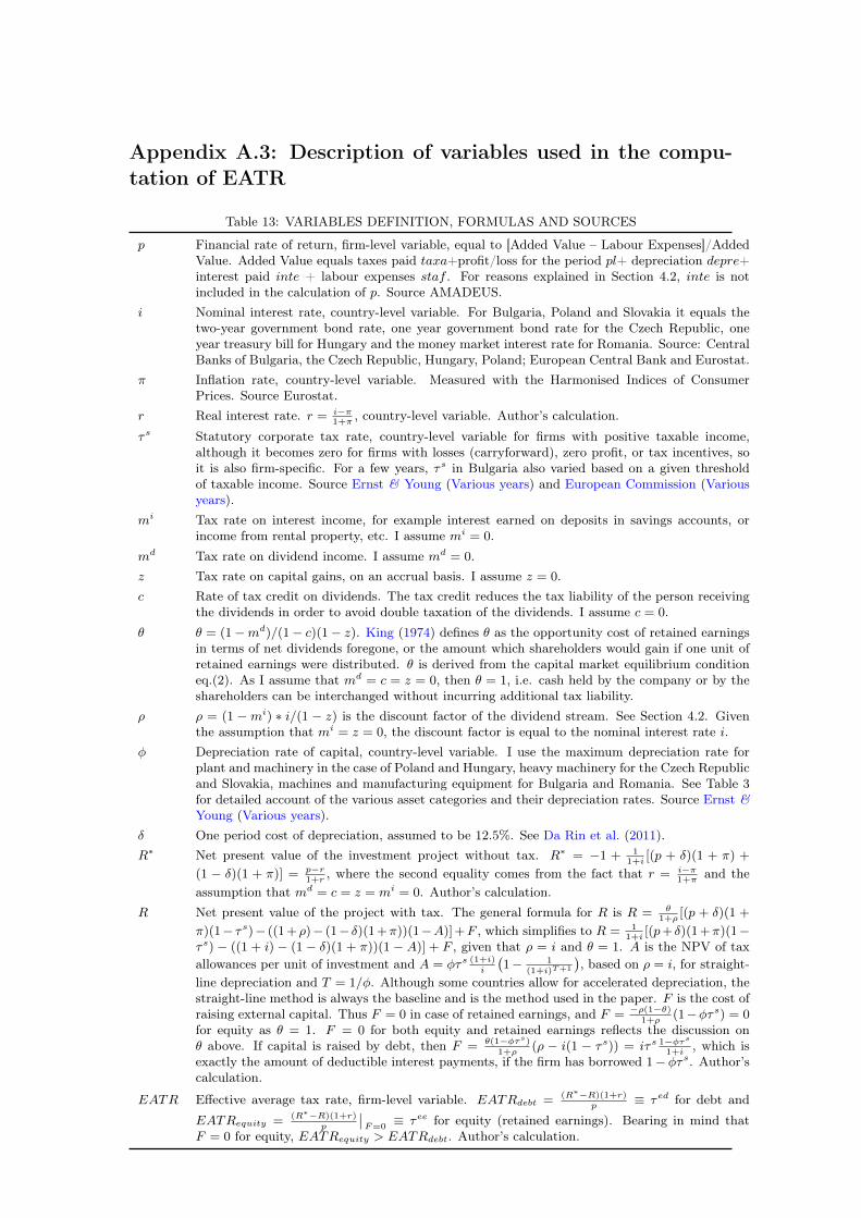
Appendix A.3: Description of variables used in the compu-tation of EATR

Table 13: VARIABLES DEFINITION, FORMULAS AND SOURCES

p Financial rate of return, firm-level variable, equal to [Added Value – Labour Expenses]/AddedValue. Added Value equals taxes paid taxa+profit/loss for the period pl+ depreciation depre+interest paid inte + labour expenses staf . For reasons explained in Section 4.2, inte is notincluded in the calculation of p. Source AMADEUS.

i Nominal interest rate, country-level variable. For Bulgaria, Poland and Slovakia it equals thetwo-year government bond rate, one year government bond rate for the Czech Republic, oneyear treasury bill for Hungary and the money market interest rate for Romania. Source: CentralBanks of Bulgaria, the Czech Republic, Hungary, Poland; European Central Bank and Eurostat.

π Inflation rate, country-level variable. Measured with the Harmonised Indices of ConsumerPrices. Source Eurostat.

r Real interest rate. r = i−π1+π

, country-level variable. Author’s calculation.

τs Statutory corporate tax rate, country-level variable for firms with positive taxable income,although it becomes zero for firms with losses (carryforward), zero profit, or tax incentives, soit is also firm-specific. For a few years, τs in Bulgaria also varied based on a given thresholdof taxable income. Source Ernst & Young (Various years) and European Commission (Variousyears).

mi Tax rate on interest income, for example interest earned on deposits in savings accounts, orincome from rental property, etc. I assume mi = 0.

md Tax rate on dividend income. I assume md = 0.z Tax rate on capital gains, on an accrual basis. I assume z = 0.c Rate of tax credit on dividends. The tax credit reduces the tax liability of the person receiving

the dividends in order to avoid double taxation of the dividends. I assume c = 0.θ θ = (1−md)/(1− c)(1− z). King (1974) defines θ as the opportunity cost of retained earnings

in terms of net dividends foregone, or the amount which shareholders would gain if one unit ofretained earnings were distributed. θ is derived from the capital market equilibrium conditioneq.(2). As I assume that md = c = z = 0, then θ = 1, i.e. cash held by the company or by theshareholders can be interchanged without incurring additional tax liability.

ρ ρ = (1 −mi) ∗ i/(1 − z) is the discount factor of the dividend stream. See Section 4.2. Giventhe assumption that mi = z = 0, the discount factor is equal to the nominal interest rate i.

φ Depreciation rate of capital, country-level variable. I use the maximum depreciation rate forplant and machinery in the case of Poland and Hungary, heavy machinery for the Czech Republicand Slovakia, machines and manufacturing equipment for Bulgaria and Romania. See Table 3for detailed account of the various asset categories and their depreciation rates. Source Ernst &Young (Various years).

δ One period cost of depreciation, assumed to be 12.5%. See Da Rin et al. (2011).R∗ Net present value of the investment project without tax. R∗ = −1 + 1

1+i[(p + δ)(1 + π) +

(1 − δ)(1 + π)] = p−r1+r

, where the second equality comes from the fact that r = i−π1+π

and theassumption that md = c = z = mi = 0. Author’s calculation.

R Net present value of the project with tax. The general formula for R is R = θ1+ρ

[(p + δ)(1 +

π)(1− τs)− ((1+ρ)− (1− δ)(1+π))(1−A)]+F , which simplifies to R = 11+i

[(p+ δ)(1+π)(1−τs) − ((1 + i) − (1 − δ)(1 + π))(1 − A)] + F , given that ρ = i and θ = 1. A is the NPV of taxallowances per unit of investment and A = φτs (1+i)

i

(1− 1

(1+i)T+1

), based on ρ = i, for straight-

line depreciation and T = 1/φ. Although some countries allow for accelerated depreciation, thestraight-line method is always the baseline and is the method used in the paper. F is the cost ofraising external capital. Thus F = 0 in case of retained earnings, and F = −ρ(1−θ)

1+ρ(1−φτs) = 0

for equity as θ = 1. F = 0 for both equity and retained earnings reflects the discussion onθ above. If capital is raised by debt, then F = θ(1−φτs)

1+ρ(ρ − i(1 − τs)) = iτs 1−φτs

1+i, which is

exactly the amount of deductible interest payments, if the firm has borrowed 1− φτs. Author’scalculation.

EATR Effective average tax rate, firm-level variable. EATRdebt = (R∗−R)(1+r)p

≡ τed for debt and

EATRequity = (R∗−R)(1+r)p

∣∣F=0

≡ τee for equity (retained earnings). Bearing in mind thatF = 0 for equity, EATRequity > EATRdebt. Author’s calculation.

Working Paper Series ISSN 1211-3298 Registration No. (Ministry of Culture): E 19443

Specific research support and/or other grants the researchers/publications benefited from are acknowledged at the beginning of the Paper. (c) Boryana Madzharova, 2012 All rights reserved. No part of this publication may be reproduced, stored in a retrieval system or transmitted in any form or by any means, electronic, mechanical or photocopying, recording, or otherwise without the prior permission of the publisher. Published by Charles University in Prague, Center for Economic Research and Graduate Education (CERGE) and Economics Institute ASCR, v. v. i. (EI) CERGE-EI, Politických vězňů 7, 111 21 Prague 1, tel.: +420 224 005 153, Czech Republic. Printed by CERGE-EI, Prague Subscription: CERGE-EI homepage: http://www.cerge-ei.cz Phone: + 420 224 005 153 Email: office@cerge-ei.cz Web: http://www.cerge-ei.cz Editor: Michal Kejak Editorial board: Jan Kmenta, Randall Filer, Petr Zemčík The paper is available online at http://www.cerge-ei.cz/publications/working_papers/. ISBN 978-80-7343-265-2 (Univerzita Karlova. Centrum pro ekonomický výzkum a doktorské studium) ISBN 978-80-7344-257-6 (Národohospodářský ústav AV ČR, v. v. i.)