Intra-national Trade Costs:Assaying Regional Frictions∗†

Delina E. Agnosteva James E. AndersonDrexel University Boston College and NBER

Yoto V. YotovDrexel University and ERI-BAS

January 19, 2015

Abstract

New methods apply gravity to flexibly infer regional, interregional and interna-tional trade costs of Canada’s provinces. A bilateral trade cost function aggregatesinterregional frictions with origin and destination region internal and border frictions.The ratio of border to intra-regional friction, the relative border friction, varies acrossregions and raises bilaterally varying Unexplained Trade Barriers (UTBs) to inter-regional trade. Small remote regions have high relative border frictions while largecentral regions have low relative border frictions. Our methods should be useful infuture investigations of non-uniform regional trade frictions and analogous barriers tomigration and direct investment.

JEL Classification Codes: F13, F14, F16

Keywords: Intra-regional Frictions, Border Frictions, Aggregation, Canada.

∗Keith Head, Mario Larch, Thierry Mayer, Peter Neary and Dennis Novy improved this paper withcomments on earlier drafts. We also thank participants of seminars at LSE, Oxford, Sciences Po andWarwick. This research is supported by the Public Policy Forum, Industry Canada, and the Internal TradeSecretariat, Canada. All errors and opinions are our own.†Contact information: Delina E. Agnosteva, School of Economics, Drexel University, Philadelphia, PA

19104, USA. James E. Anderson, Department of Economics, Boston College, Chestnut Hill, MA 02467, USA.Yoto V. Yotov, School of Economics, Drexel University, Philadelphia, PA 19104, USA. Economic ResearchInstitute, Bulgarian Academy of Sciences, Sofia, Bulgaria.

1 Introduction

A national economy is composite rock, discrete regions connected with varying strength to a

matrix of interregional and international ties. A flexibly specified structural gravity method

crunches trade flow data for an assay. A feature of the approach identifies each region’s

resistance at its border relative to its intra-regional trade friction, based on specifying a

bilateral trade cost function that aggregates origin and destination intra-regional, regional

border and pure interregional frictions. The results are consistent with regionally varying

intra-regional trade costs and regional border barriers of varying thickness. The trade of small

remote provinces is suppressed relatively more, controlling for variation of intra-national

bilateral distance and size. Our methods and data are applied to 19 goods and 9 service

sectors for Canada from 1997-2007. Previous investigations of intra-national border effects

have been constrained by limited data and techniques mainly to price comparisons that

cover a relatively small proportion of trade. Variation in distribution costs internal to the

origin and destination coordinates of observation (regions or countries) is often suppressed

in gravity models, but is generally consequential for distinguishing border effects and for

comparative statics. Ramondo et al. (2014) emphasize that variation of internal trade costs

helps resolve puzzles in the open economy macro literature.1 Thus our methods are a useful

extension of structural gravity to many types of questions to which it has been applied.

Intra-national trade cost structure comprises components of pure intra-regional, regional

border and pure interregional costs. Our method disentangles them with a cost aggrega-

tion structure for the components combined with inference from two estimated variants of

structural gravity. One variant uses bilateral fixed effects along with importer-time and

exporter-time fixed effects to measure volume effects of trade costs for Canada’s provinces.2

1Due to scale effects, endogenous growth models imply that larger countries should be richer than smallercountries. Similarly, standard trade models imply that real income per capita (domestic trade shares andrelative income levels) increases too steeply with country size. Ramondo et al. demonstrate that these coun-terfactual implications are mitigated/disappear when the standard, but unrealistic, assumption of frictionlessdomestic trade is relaxed. Our methods of identifying internal frictions extend and complement theirs.

2Previous literature (including our own) has used the somewhat suspect concept of internal distance toproxy for internal frictions, imposing a uniform distance elasticity to provide sufficient degrees of freedom.

1

The other variant estimates volume effects from bilateral distance and contiguity along with

importer-time and exporter-time fixed effects and a set of fixed effects for intra-regional

trade.

The difference between the pair fixed effect and the fitted bilateral distance/contiguity

effect is the Unexplained Trade Barrier (UTB). Unexplained Trade Barrier variation across

regions is due to the volume effects of relative border frictions: the ratio of internal dis-

tribution costs to regional border costs in both origin and destination regions varies across

regions.3 The systematic portion of UTBs and the effect of the non-uniform provincial rela-

tive home bias is identified from a precisely estimated second stage regression of first stage

bilateral fixed effects on the elements of the first stage gravity variables estimates. Identifica-

tion of the relative home bias effects utilizes a Cobb-Douglas trade cost function to aggregate

internal and interregional costs into full bilateral trade costs. UTBs could alternatively or

additionally reflect a trade cost function more general than Cobb-Douglas. A translog test

gives no support for rejecting the Cobb-Douglas specification.

We apply the structural gravity model to high quality provincial trade flow data4 over

the period 1997-2007. The discussion of results concentrates on estimates from aggregate

manufacturing bilateral trade for simplicity. The results are qualitatively similar to those for

the 19 goods and 9 services sectors briefly discussed.5 Estimates are quite precise. Analysis

of residuals and sensitivity experiments support our baseline specification.

Regionally varying internal trade fixed effects gain adequate degrees of freedom by judicious use of panelstructure.

3“Unexplained” here applies Head and Mayer’s (2013a) cosmological metaphor: gravity trade costs aredark. This paper moves the darkness one step by identifying systematic effects of border costs relativeto internal costs, but shadow covers what these costs may be. More shadow covers intra-regional coststhat are themselves aggregates across trade costs between smaller sub-regions. The darkness metaphor alsoacknowledges that “costs” in the usage of this paper (and much of the literature) may be resistance tointer-regional and international trade due to “buy local” bias of buyers.

4The paucity of research on intra-national trade costs is partly due to deficient data. To our knowledge,except for Canada, data on bilateral shipments within nations does not record true origin-destination trade.In particular, the widely used US Commodity Flow Survey does not control for entrepot trade.

5Details are available on request, but we see the sectoral estimates as an input to investigate the rela-tionship between border barriers and institutional and infrastructure variables, or for general equilibriumcomparative statics. Sectoral disaggregation is generally important because previous work (Anderson andYotov (2010)) has shown that estimates of trade costs from aggregate data are biased downward, a concernespecially acute for estimating intra-national trade costs.

2

The more remote and smaller regions (e.g. YT, PE, and NT) are systematically subject to

the largest UTBs. The effects of border barriers are measured relative to a national average,

so economically developed and central regions (e.g. ON, AB, and BC) enjoy relative stimuli

to trade from UTBs.6 At one extreme, PE exports to YT are reduced 43% by their 2002

UTB in manufacturing. At the other extreme, ON exports to BC are raised 30% by their

UTB. The details of variation across provinces and provincial pairs may indicate where policy

intervention is needed most. The pattern of UTBs is also consistent with intra-regional cost

variation because regions with larger internal distances (measured with the CEPII method)

tend to have more trade, all else equal. Disentangling internal from border cost variation is

an important but difficult task for future work.

Overall measures of resistance to interregional trade combine direct frictions (intra-

regional and border frictions and pure interregional frictions) with the general equilibrium

effects of multilateral resistance. Constructed Trade Bias (CTB) is the ratio of predicted

(including multilateral resistance) to hypothetical frictionless trade flows for each bilateral

pair. CTBs (consistently aggregated across provincial partners) in 2002 range from 14.2

for SK down to 2.3 for YT, confirming the familiar result of ‘excess’ interprovincial trade.

The ratio of interregional to intra-regional CTB is Constructed Interregional Bias (CIB).

CIB is transformed to a relative cost measure, the ratio of sellers’ incidence of interregional

trade costs to sellers’ incidence of intra-regional trade costs. The transformation is based on

estimated CIBs raised to the power 1/(1− σ) with elasticity of substitution σ = 5. Relative

sellers’ incidence in 2002 manufacturing ranges from 13.2 for Yukon Territory down to 1.2

for Ontario. Variation is even greater across provincial partners for each exporter.

Canada’s provinces are mostly becoming more integrated with both the world and with

each other over the period 1997 to 2007, despite the constant bilateral trade costs that we

find. Intra-regional CTB (Constructed Home Bias) is falling, provinces are becoming more

6The provincial border barriers are inferred as deviations around a Canada-wide mean, so low borderbarrier provinces tend to enjoy relative stimulus due to the UTB. Due to collinearity we are unable tomeasure the level of border barriers, only the variation.

3

integrated with the world (extending Anderson and Yotov (2010)). The fall in CHBs is

largest for the remote regions YT (79%) and NT (62%). The small exceptions are BC and

NB with increases of 2% and 4.2% respectively. Interregional CTBs are mostly rising. The

exceptions are YT (-83.8%) and NT (-41.3%) along with small falls in ON (-7.8%) and MB

(-0.8%). CIB rises for all but YT (-4.8%), Canada’s provinces are becoming more integrated.

Increasing integration intra-nationally and internationally is due to changes in the incidence

of trade costs that in turn are due to changes in location of production and expenditure.7

We depart from the existing literature on intra- and interregional trade costs in allowing

maximum flexibility of estimated intra-regional and interregional trade costs.8 We allow for

non-uniform intra-regional trade costs, non-uniform regional border barriers and estimate

a combination of them along with inter-regional trade costs. International border barriers

are not our focus, though our estimation utilizes international as well as interregional trade

flows. The flexible treatment of trade costs enables identification of the effects of provincial

border variation on bilateral trade with potential implications for regional trade policy.

Tombe and Winter (2014) share our focus on intra-national Canadian trade costs inferred

from gravity, but differ in not being able to identify provincial border barriers.9 They infer

7See Anderson and Yotov (2010) for a discussion of the effect of changes in location of production andexpenditure on incidence.

8For the United States see Wolf (2000), Head and Mayer (2002), Hillberry and Hummels (2003), Mil-limet and Osang (2007), Head and Mayer (2010), Coughlin and Novy (2012), Yilmazkuday (2012)); for theEuropean Union see Nitsch (2000), Chen (2004), and Head and Mayer (2010); for OECD countries (Wei(1996)); for China see Young (2000), Naughton (2003), Poncet (2003, 2005), Holz (2009), Hering and Poncet(2010); for Spain see Llano and Requena (2010); for France see Combes et al. (2005); for Brazil see Fallyet al. (2010); and for Germany see Lameli et al. (2013) and Nitsch and Wolf (2013). A summary tablethat reviews home bias estimates is available by request. This literature has mainly adopted two methodsof estimating internal trade barriers: using the gravity model with a uniform effect of intra-regional relativeto inter-regional trade costs or using proxies for inter-regional trade borders. A more distantly related liter-ature infers trade costs from price differences (e.g., Engel and Rogers (1996)) at a much more disaggregatedlevel. As with trade flows, distance and borders account well for price differences. Very highly detailed pricecomparisons often imply very large intra-national price gaps in developing countries (Atkin and Donaldson(2013)); much less so in developed countries. The price comparison method is limited in coverage due tothe difficulty of matching prices for truly comparable items across locations. Trade flow inference includessubstitution on the extensive margin that price comparison necessarily excludes. Moreover, price comparisoncan only find trade costs that show up in prices, in contrast to inference from trade flows that includes allnon-price costs borne by buyers (travel time, contracting costs, etc.). Inference from trade flows providescomplementary evidence on trade costs for these reasons.

9Our work is more remotely related to the literature on the international border barrier to Canada’s trade:e.g., McCallum (1995), Anderson and van Wincoop (2003). Apart from gravity, a number of case studies

4

pure inter-regional trade costs from observed bilateral trade relative to the geometric mean of

origin and destination internal trade using the “tetrads” approach of Head and Mayer (2000).

By construction tetrads includes random elements excluded from our fitted pairwise fixed

effects estimator. The two estimators are highly correlated, though the fixed effects estimates

differ significantly from their tetrads counterparts in the statistical sense. Tombe and Winter

(2014) then infer bilateral frictions apart from distance by parametrically removing bilateral

distance effects. This resembles our difference between estimated bilateral pair fixed effects

and estimated standard gravity variables. But our second stage regression allows us to

identify variation in provincial border effects and to decompose UTBs into border effects

and unexplained components.

Our methods should be applicable widely to flexible inference of intra-national trade costs

and international border barriers in multi-country and multi-regional studies. The flexible

fixed effects treatment of trade costs can also be applied to quantify barriers to immigration

and FDI, about which we know much less than about trade costs. The methods can be used

to decompose those barriers to isolate border effects with implications for immigration and

FDI policy.

Section 2 sets out the theoretical foundation and introduces Constructed Trade Bias

indexes. Section 3 describes our data and presents the econometric specification and identi-

fication strategy. Section 4 presents our main findings and sensitivity experiments. Section

5 discusses sectoral estimates. Section 6 concludes.

2 Theoretical Foundation

A review of structural gravity theory (Anderson and van Wincoop (2003, 2004)) sets the

stage for extensions. Next, we define Constructed Trade Bias (CTB), the generator of

have also examined the economic costs of internal trade barriers in Canada. Grady and Macmillan (2007)provide a descriptive overview of the academic and non-academic literature on barriers to internal trade inCanada and also evaluate the economic costs brought about these impediments to trade. Beaulieu et al.(2003) describe in great detail the various trade policies and reforms initiated by the Canadian governmentin order to liberalize inter-provincial trade.

5

a family of Constructed Bias indexes with two novel ones useful for understanding intra-

national trade. Then we analyze bilateral trade costs as a combination of intra-regional and

pure interregional costs, developing implications for comparative statics and econometric

identification. Finally, consistent aggregation of bilateral trade costs is developed.

The structural gravity model assumes identical preferences or technology across countries

for national varieties of goods or services differentiated by place of origin for every good or

service category k, represented by a globally common Constant Elasticity of Substitution

(CES) sub-utility or production function.10 Use of the market clearing condition for each

origin’s shipments and each destination’s budget constraint yields the structural form:

Xkij =

Ekj Y

ki

Y k

(tkij

P kj Πk

i

)1−σk

(1)

(Πki )

1−σk =∑j

(tkijP kj

)1−σkEkj

Y k(2)

(P kj )1−σk =

∑i

(tkijΠki

)1−σk

Y ki

Y k, (3)

where Xkij denotes the value of shipments at destination prices from region of origin i to

region of destination j in goods or services of class k. The order of double subscripts denotes

origin to destination. Ekj is the expenditure at destination j on goods or services in k from

all origins. Y ki denotes the sales of goods or services k at destination prices from i to all

destinations, while Y k is the total output, at delivered prices, of goods or services k. tkij ≥ 1

denotes the variable trade cost factor on shipments of goods or services from i to j in class

k, and σk is the elasticity of substitution across goods or services of class k. P kj is the inward

multilateral resistance (IMR), and also the CES price index of the demand system. Πki is

the outward multilateral resistance (OMR), which from (2) aggregates i’s outward trade

costs relative to destination price indexes. Multilateral resistance is a general distributional

10Two alternative theoretical foundations for (1)-(3) feature selection — substitution on the extensivemargin in either supply or demand. See Anderson (2011) for details. In practice, either type of substitutionor both may be the interpretation.

6

equilibrium concept, since {Πki , P

kj } solve equations (2)-(3) for given {Y k

i , Ekj }.

The right hand side of (1) comprises two parts, the frictionless value of trade Ekj Y

ki /Y

k

and the distortion to that trade induced by trade costs (tkij/ΠkiP

kj )1−σk directly with tkij and

indirectly with ΠkiP

kj . Anderson and Yotov (2010) note that P k

j and Πki are respectively

the buyers’ and sellers’ overall incidence of trade costs to their counter-parties worldwide.

Incidence here means just what it does in the first course in economics: the proportion of the

trade cost factor tkij paid by the buyer and seller respectively. The difference is that purchase

and sales are aggregated across bilateral links, such that conceptually it is as if each seller’s

global sales travel to a hypothetical world market with equilibrium world price equal to 1.

The seller receives 1/Πki , hence pays incidence factor Πk

i . Each buyer makes purchases from

all origins on the world market, paying incidence P kj to bring them to destination j. These

overall incidence measures further imply bilateral incidence: tkij/Pkj is seller i’s incidence of

trade costs on sales to destination j for good k, and tkij/Πki is buyer j’s incidence of trade

costs on purchase from origin i for good k. tkij/ΠkiP

kj is interpreted as either bilateral buyer’s

incidence, (tkij/Πki )/P

kj relative to overall buyers’ incidence, or bilateral sellers’ incidence

(tkij/Pkj )/Πk

i relative to overall sellers’ incidence.

2.1 Constructed Trade Bias

Constructed Trade Bias is defined as the ratio of the econometrically predicted trade flow

Xkij to the hypothetical frictionless trade flow between origin i and destination j for goods

or services of class k. Rearranging the econometrically estimated version of equation (1),

Constructed Trade Bias is given by:

CTBkij ≡

Xkij

Y ki E

kj /Y

k=

(tkij

Πki P

kj

)1−σk

. (4)

In the hypothetical frictionless equilibrium CTBkij = 1, i’s share of total expenditure by each

destination j,Xkij/E

kj , is equal to Y k

i /Yk, i’s share of world shipments in each sector k. This

7

would be the pattern in a completely homogenized world. “Frictionless” and “trade costs”

are used here for simplicity and clarity, but the model can also reflect local differences in

tastes that shift demand just as trade costs do, suggesting “resistance” rather than costs.

The second equation in (4) gives the structural gravity interpretation of CTB, the 1 − σk

power transform of the ratio of predicted bilateral trade costs to the product of outward

multilateral resistance at i and the inward multilateral resistance at j. (The Constructed

Home Bias index of Anderson and Yotov (2010) is the special case CTBkij; i = j home bias

of i’s internal trade.)

Five properties of CTB are appealing. First, CTB is independent of the normalization

needed to solve system (2)-(3) for the multilateral resistances.11 Second, CTB is independent

of the elasticity of substitution σk, because it is constructed using the inferred (estimated)

volume effects that are due to 1 − σk power transforms of the tkij’s, the Πk’s and the P k’s.

Third, CTB can be consistently aggregated to yield a family of useful general equilibrium

trade costs indexes at the country and at the regional level. One is developed below to

measure aggregate inter-regional trade bias facing sellers.12 Fourth, because it measures the

proportional displacement of volume from the observable frictionless benchmark, CTB is

comparable across sectors and time as well as across provinces and countries.13 Fifth, CTB

infers central tendency out of the random errors that beset notoriously mis-measured bilateral

trade flow data. Specifically, the ratio of observed bilateral trade to hypothetical frictionless

trade is an observation of CTB while our estimated CTB is its conditional expectation. CTB

shares the good fit properties of gravity models, so this distinction is important.

Intra-provincial and inter-provincial trade both are raised relative to their frictionless

benchmark values by large international trade costs, but intra-provincial trade is increased by

11Note that (2)-(3) solves for {Πki , P

kj } only up to a scalar. If {Π0

i , P0j } is a solution then so is {λΠ0

i , P0j /λ}.

12Other CTB aggregates have been defined and reported in Anderson and Yotov (2010) and Anderson,Milot and Yotov (2013).

13In contrast, because gravity can only identify relative bilateral trade costs, constructed trade costsdepend on normalizations by unobservable levels of bilateral cost that in principle vary across sectors andtime, vitiating comparability along these dimensions. The same issue arises with the multilateral trade cost(multilateral resistance) measures that can be inferred from structural gravity.

8

much more. To focus on internal barriers to trade, a useful and natural index is Constructed

Interregional Bias (CIB):

CIBkij = CTBj

ij/CTBkii =

(tkij/P

kj

tkii/Pki

)1−σk

=

(tkijtkii

)1−σk

/

(P kj

P ki

)1−σk

. (5)

In a frictionless world, CIBkij = 1 = CTBk

hl,∀h, i, j, k, l. The left hand side of equation (5)

gives the relative reduction of inter-provincial trade due to trade costs in the world system.

The middle equation gives CIB as the 1− σk power transform of seller i’s incidence on sales

to j relative to i’s internal sales. The rightmost equation breaks the ratio into the 1 − σk

power transforms of two components. The numerator component is the interprovincial part

of the total shipment cost from i to j, tkij/tkii. The denominator component is P k

j /Pki , the

additional buyer’s incidence facing seller i when selling to destination j.

2.2 Modeling Full Bilateral Costs

The composition of full bilateral costs has usually been submerged in the gravity literature.

Intra-regional or intra-national costs and their relation to full costs are omitted without

apparent effect on inference of bilateral costs modeled as iceberg log linear functions of

geographic proxies.14 In contrast, intra-national costs are consequential for comparative

statics and regional policy analysis. In particular, regional border barriers are a key concern

of this paper.

Time-invariant components of bilateral trade frictions are estimated alternatively with

bilateral fixed effects (identified off the time variation of panel data) and with a log-linear

function of geographic proxies. The difference between the fixed effects and gravity variables

estimates is the Unexplained Trade Barrier. Systematic variation in the estimated UTBs

due to border barriers is identified based on a structural relationship between intra-regional

14An exception is the Helpman, Melitz and Rubinstein (2008) specification that includes a fixed exportcost component. Their identification strategy to distinguish variable from fixed cost uses common religionto determine fixed but not variable cost, controversial in any case but unavailable for Canada’s provinces.

9

and interregional cost components. Idiosyncratic components of UTBs may contain bilateral

border barrier information, but also contain random error.

Full interregional trade costs are modeled as a degree one homogeneous increasing and

concave function tij = g(rij, rii, rjj) of three components, the resource costs (rhl, ∀h, l) of

delivering one unit of distribution activity within the origin, destination and transit between

them respectively. (In the Ricardian case rij = waij where w is the wage and aij is the unit

labor requirement in activity ij.) Homogeneity of degree one is consistent with iceberg trade

costs with no indivisibilities. Concavity is implied by cost-minimizing behavior. The base

case is the Cobb-Douglas specification

tij = rρ1ij rρ2ii r

ρ3jj , (6)

where ρ1 + ρ2 + ρ3 = 1.

The base case simplifies identifying border barriers. If the full cost of i shipping to j

includes border crossing components b(i), b(j), their effect on full cost is b(i)ρ2b(j)ρ3 . The

border crossing costs are combined with the pure intra-regional costs in the estimation, but

identification of the border costs (up to a normalization) is made possible by the structure,

as shown in Section 4.2

The Cobb-Douglas restriction yields a very useful theoretical property: system (1)-(3) is

neutral with respect to (invariant to) intra-regional trade costs. Neutrality follows because

rρ2ii , rρ3jj form part of the composite multilateral resistances r−ρ2ii Πi , r

−ρ3jj Pj that solve (2)-

(3), hence the composite multilateral resistances are invariant to the level of intra-regional

trade costs. In the econometric specification of bilateral trade costs below, the composite

multilateral resistance terms are controlled for with origin and destination fixed effects and

the bilateral cost identified is the pure inter-regional cost. Comparative static effects of

intra-regional trade costs in the Cobb-Douglas case are confined to upper level inter-sectoral

allocation due to invariance of (2)-(3) for given Es and Y s.

10

Neutrality is violated by general cost function specifications g(·). For example, in the

translog case ln(tij/ΠiPj) decomposes into the Cobb-Douglas invariance term analyzed above

plus a second order effect term that contains the intra-regional trade cost. Non-neutrality

implies that intra-regional trade cost changes affect all bilateral trade patterns by changing

all the multilateral resistances. Evidence below is weakly consistent with rejecting non-

neutrality. Future work should probe further for possible non-neutrality.

2.3 Consistent Aggregation of Trade Bias and Trade Costs

Aggregation of volume concepts such as CTBs and trade cost concepts such as multilateral

resistance and tij or tij/tii is useful for many purposes. Aggregation procedures are set out

here for CTBs and multilateral resistances that are consistent with maintaining a constant

aggregate volume of trade given the theoretical model. (Volume consistent trade cost ag-

gregation can be done following Anderson and Neary (2005), pp. 177-83.) Aggregation over

regions is the focus, but similar principles apply to consistent aggregates over sectors.

The aggregate (export) trade volume from origin i to some subset of destinations C(i) =

{j ∈ C, j 6= i} is ∑j∈C(i)

Xij =∑j∈C(i)

YiEjY

(tij

ΠiPj

)1−σ

. (7)

C(i) excludes internal trade, and can also exclude other bilateral trade depending on what

is defined to be contained in C. In the present application, C designates within country C

(Canada), so it excludes international trade, thus C(i) is the set of interprovincial partners

of province i. Constructed Trade Bias for i’s export trade to C(i) is given by the ratio of

the theoretical aggregate volume given above to the frictionless benchmark aggregate export

volume YiEC(i)/Y where EC(i) ≡∑

j∈C(i) Ej. Using equation (4), the ratio is equal to

CTBC(i) =∑j∈C(i)

EjEC(i)

CTBij. (8)

11

The aggregate CTB for set C (Canada’s overall CTB for interprovincial trade) is given by

CTBC =∑i∈C

EC(i)

ECCTBC(i) =

∑i∈C

∑j∈C(i)

EjEC

CTBij, (9)

where EC =∑

iEC(i).15

The CTBC(i) concept is illustrated by Canadian province i’s interprovincial exports, but

can be applied to any arbitrary set of regions’ interregional exports or, mutatis mutandis,

to imports rather than exports.16 For example, the concept can usefully be applied to

preferential trade arrangements.

The aggregate CIB for region i is defined as CIBC(i) ≡ CTBC(i)/CTBii. CIBC(i) mea-

sures the average amount by which trade costs directly and indirectly reduce interregional

volume relative to intra-regional volume for region i with its partners in C. The aggregate

CIB for set C is given by CIBC/[∑

iCTBiiEi/EC ].

Turning to relative cost counterparts to the aggregate volume concepts, power transforms

of the CIBs give relative sellers’ incidence measures, just as in equation (5). This follows

because CTBC(i) =∑

j∈C(i)(tij/Pj)1−σEj/EC(i) = Π1−σ

C(i) where the first equation follows by

substituting (1) into (4) and (29), and the second equation formalizes the interpretation of

the result by defining the sellers’ incidence of i on sales to C(i). Π1−σC(i) is the expenditure

weighted average of the volume effect of the bilateral sellers’ incidences (tij/Pj)1−σ. Then

the region i’s sellers’ incidence on sales to C(i) relative to local sales is given by:

ΠC(i)

Πii

=(CIBC(i)

)1/(1−σ), (10)

where Πii ≡ tii/Pi. The relative incidence measure (10) is the economic driver of the volume

response of the sellers, CIBC(i), representing how the system of bilateral trade costs directly

and indirectly determines seller behavior.

15The Constructed Foreign Bias (CFB) and the Constructed Domestic Bias (CDB) indexes of Andersonet al. (2013) are focused on aggregation across destinations to measure outward resistance to trade.

16In the import case, the expenditure share weights are replaced by sales share weights.

12

3 Empirical Foundation

This section details the econometric specification and procedures used to infer the volume

displacement and trade cost indexes describing inter-provincial trade in Canada. An exten-

sion of now standard gravity methods that exploits the panel nature of the data permits

measurement of potential unobservable barriers at provincial borders — Unexplained Trade

Barriers (UTBs). The section closes with a brief description of our data, supplemented by a

detailed Data Appendix.

3.1 Econometric Specification

The fixed effects econometric approach estimates Constructed Trade Biases for each pair of

regions and each year in the sample directly (except where necessary the sectoral index k is

suppressed):

xij,tYtYi,tEj,t

= exp[α′Tij,t + γij + ηi,t + θj,t] + εij,t. (11)

The dependent variable is size-adjusted trade. Hence the CTB is the predicted value from

(11). The last two terms in the square brackets of (11) account for the structural multilateral

resistances. Specifically, ηi,t denotes the set of time-varying source-country dummies that

control for the unobservable outward multilateral resistances and any other time varying

source country factors, and θj,t encompasses the time varying destination country dummy

variables that account for the inward multilateral resistances and any other destination

country factors. The first two terms on the right hand side of equation (11) account for

bilateral trade costs.

Bilateral trade costs in (11) are decomposed into time-dependent and time-invariant

components:

(tFEij,t)1−σ

= exp[α′Tij,t + γij]. (12)

13

Here, tFEij,t denotes bilateral trade costs between regions i and j at time t, and the superscript

FE captures the fact that we use the full set of pair-fixed effects, γij, to account for the

time invariant portion of trade costs. In addition to absorbing the vector of time-invariant

covariates that are used standardly in the gravity literature (e.g. distance), the pair-fixed

effects will control for any other time-invariant trade costs components that are unobservable

to researchers and to policy makers.17

The first term in (12), Tij,t, is a vector of time-varying gravity variables intended to

capture changes in bilateral trade costs over time. The changes are restricted to sensibly

pick up suspected effects.18 The evolution of internal trade costs in Canada is captured

by two time-varying covariates. INTRAPR Tij,t = INTRAPRij × Tt is the interaction

between a dummy variable for intra-provincial trade INTRAPRij and a time trend Tt. The

estimated coefficient of INTRAPR Tij,t would capture any changes in intra-provincial trade

costs over the period of investigation. Similarly, INTERPR Tij,t = INTERPRij×Tt is the

interaction of INTERPRij, a dummy variable for inter-provincial trade with a time trend,

and its estimated coefficient has a similar interpretation. By construction, the estimated

coefficients of INTERPR Tij,t and INTRAPR Tij,t should be interpreted as deviations

of internal (intra-provincial or inter-provincial) Canadian trade costs from the changes in

international trade costs over time.

With these restrictions, specification (11) becomes:

xij,tYtYi,tEj,t

= exp[α1INTERPR Tij,t + α2INTRAPR Tij,t + γij + ηi,t + θj,t] + εij,t. (13)

The benefit of using pair-fixed effects in specification (13) is that these fixed effects control

17Using bilateral fixed effects in the gravity equation is not new. For example, Baier and Bergstrand (2007)use pair fixed-effects to successfully account for potential endogeneity of FTAs. However, to the best of ourknowledge, ours is the first paper to use bilateral pair fixed effects to properly measure bilateral trade costs.More importantly, as emphasized below, we are the first to construct and to study the difference betweenthe trade costs from the fixed effects specification, and the trade costs from a standard specification withgravity variables.

18The usual components of Tij,t, when the gravity model is applied to international trade data, control fortariffs, for the presence of free trade agreements (FTAs), monetary unions (MUs), World Trade Organization(WTO) membership, etc. Given the specifics of our sample, we cannot include any of these variables.

14

for all possible time-invariant bilateral trade costs. The estimates of the bilateral trade costs

from (13) are in principle directly comparable to estimates of trade costs that are obtained

from a specification with standard gravity variables. We exploit the comparability below to

construct the Unexplained Trade Barriers estimate as the difference between the two.

Perfect collinearity requires restrictions on the pair-fixed effects in order to estimate spec-

ification (13).19 Perfect collinearity arises because the sum of the dummy variable vectors

corresponding to the full set of γijs is equal to the sum of dummy variable vectors corre-

sponding to the full set of province dummies, either as exporter or importer.

The restriction we impose scales the time-invariant bilateral trade costs so that inter-

nal trade costs are suppressed: interprovincial trade costs are measured relative to intra-

provincial costs. The restriction relates γij from a theoretical original set of Γijs subject to

γij = Γij − (ζOΓii + ζDΓjj) ⇒ γii = γjj = 0. Here ζO ≥ 0, ζD ≥ 0, ζO + ζD = 1 are unob-

served weights interpreted within the Cobb-Douglas cost assumption as ζO = ρ2/(ρ2 + ρ3)

for Origin internal cost and ζD = ρ3/(ρ2 + ρ3) for Destination internal cost. The estimated

bilateral fixed effects for interprovincial trade are thus understood as relative to an index of

intra-provincial fixed effects: exp(γij) = exp[Γij−(ζOΓii+ζDΓjj)] = [rρ1ij /(rρ2ii r

ρ3jj )]

(1−σ)/(ρ2+ρ3).

A second restriction is to impose symmetry on the interprovincial fixed effects: γij =

γji;∀i, j ∈ CA.20 The symmetry restriction is imposed for comparability with the necessarily

symmetric gravity variables specification. In contrast we do not impose any restrictions on

trade costs between the Canadian regions, the U.S. and the rest of the world. This helps

control for complications and biases associated with measuring trade costs among these

aggregate regions.21

19Another collinearity problem, which is standard in gravity estimations, arises because the sum of theprovince/territory dummy variable vectors corresponding to origin and destination regions respectively areequal to each other in each period. This problem is solved by dropping one province as a destination in eachyear, meaning that the remaining province origin and destination coefficients for that period are interpretedas relative to the coefficient of the dropped province. To use a constant term, the same province is alsodropped once as an origin.

20In robustness checks, allowing for asymmetry of pairwise fixed effects has little effect on results.21In the Supplementary Appendix, we demonstrate that our internal trade costs estimates are robust to

the exclusion of the U.S. and the rest of the world in our sample.

15

Under the restrictions, the inter-provincial volume effects of trade costs from specification

(12) are: (tFEij)1−σ

= [rρ1ij /(rρ2ii r

ρ3jj )]

(1−σ)/(ρ2+ρ3) = eΓij/e(ζOΓii+ζDΓjj) = eγij , (14)

where the last equality reflects the estimated value. Given separately obtained estimates

of the intra-regional trade costs, the full interregional volume effect t1−σij = exp(Γij) can be

obtained. Alternatively,(tFEij)1−σ

= eγij is interpreted as trade volume displacement due

to inter-regional (interprovincial) trade costs relative to the Cobb-Douglas index of intra-

regional trade costs. The corresponding tariff equivalent index is:

τFEij =(eγij/(1−σ) − 1

)× 100, (15)

where, σ is the trade elasticity of substitution. Following the existing literature, in our

empirical analysis we choose the standard value for the elasticity of substitution σ = 5.22

Fixed effects specification (14) is related in theory to the tetrads measure proposed by

Head and Mayer (2000) and used since by others. Using only observables, they propose√XijXji/XiiXjj as representing [tij/(tiitjj)

1/2]1−σ. The theoretical difference is that ζO 6=

ζD 6= 1/2, though in practice for our Canadian manufacturing data the estimated values are

close to 1/2. The more important practical difference with our bilateral fixed effects approach

is that our estimated γij is fitted, controlling for random errors, whereas the tetrads ‘estimate’

includes the error terms. Moreover, specification (13) controls for origin- and destination-

time effects in the random errors. Tests below indicate that the tetrads estimator and the

pairwise fixed effects estimator are close economically but differ statistically.

The gravity counterpart to(tFEij)1−σ

in equation (17) is:

(tGRAVij,t

)1−σ= exp[α′Tij,t + (1− δij)β′GRAVij + δijψii]. (16)

22In the sensitivity analysis, we experiment with σ = 3 and σ = 7.

16

Here, GRAVij is a vector of time-invariant covariates that replace the vector of pair-fixed

effects γij from specification (12) for i 6= j and δij is the Kronecker delta. The explanatory

variables in GRAVij include the logarithm of bilateral distance between partners i and

j, and a contiguity indicator for whether or not the two trading regions share a common

border. The gravity variables regression continues to use a pair fixed effect for provincial

flows to or from the US and the ROW (Rest of the World). Since the inter-provincial fixed

effects for i 6= j are replaced with observable variables, it is feasible to estimate the full set

of intra-provincial fixed effects ψii, which now appear explicitly in specification (16).

The intra-provincial fixed effect ψii is a ‘relative home bias’ index that controls for intra-

regional cost relative to the provincial border effect that is implicitly absorbed in specification

(16). Moreover, this provincial border effect is measured relative to all bilateral trade after

controlling for distance and contiguity, so it is implicitly normalized by an economy wide

average border cost.23 The theoretical interpretation of the intra-provincial fixed effect (up to

a normalization) is ψii = (1− σ) ln[tii/(b(i)/b)ρ2)] where tii denotes the true intra-provincial

trade cost, b(i) the provincial border cost and b the national average border cost.

To compare bilateral trade volume effect estimation results from the full fixed effect

estimator to results from the gravity variables estimator, estimated ψiis must be used to

adjust the(tGRAVij,t

)1−σestimates. Specifically, ignoring the time dimension, the adjusted

inter-provincial trade costs from specification (16) are [tGRAVij /(tζOii tζDjj )]1−σ. The t1−σii s are

not directly inferred from ψii unless there are no border effects, but our procedures below

handle this problem.

The Unexplained Trade Barrier (UTB) is defined as the difference between the logarithm

of the volume effect of bilateral trade costs constructed from the specification with fixed

23This combined effect arises because the indicator variable for i’s internal trade measures internal relativeto interprovincial trade, all else equal. Specification (16) is constructed without regional border indicatorvariables due to collinearity. In principle, the ψii estimates can be regressed on various potential determinantsof domestic trade costs. We defer this investigation to future work. Using internal log distance measures forthe 12 provinces plotted against the estimated ψiis reveals a positive slope, suggesting important variationas is intuitive. But the data is too weak to use believably to decompose sources of variation in ψii. Indeed,even this positive distance elasticity emerges only after excluding outliers YT and PE, which are relativelycompact and small in population.

17

effects,(tFEij,t)1−σ

, and the corresponding trade costs obtained from a specification where

the pair-fixed effects γij from specification (12) are replaced with gravity variables such as

distance and contiguity. Formally, the Unexplained Trade Barrier is defined as:

lnUTBij,t = ln(tFEij,t)1−σ − ln

(tGRAVij,t /[(tGRAVii,t )ζO(tGRAVjj,t )ζD ]

)1−σ+ νij,t. (17)

On the right hand side, the interregional cost estimated from gravity variables is measured

relative to the Cobb-Douglas mean intra-regional cost, to make it consistent with the inferred

measure from bilateral fixed effects under the dropped variable specification above. νij,t is

a residual. At a minimum, analysis of variance of (17) gives a measure of how well the

standard parsimonious gravity treatment of trade costs performs.24 But more structure can

be identified from a second stage regression based on (17) using the Cobb-Douglas full trade

cost specification. The coefficients ζO ,ζD are identified and the slopes of the gravity variables

first stage estimates reveal systematic effects of provincial borders, as shown in Section 4.2.

The general equilibrium volume effects of trade costs are captured by Constructed Trade

Bias estimates. We construct CTBs using the pair-fixed effects gravity specification (13).

The corresponding Constructed Trade Bias (for a generic sector) is:

CTBij,t =(tij

Πi,tPj,t

)1−σ

= exp[α1INTERPR Tij,t + α2INTRAPR Tij,t + γij + ηi,t + θj,t](18)

The CTB measure (18) can be compared across sectors and over time because it is a pure

volume displacement ratio, predicted volume relative to an observable frictionless bench-

mark. We capitalize on the sectoral dimension of our data to study CTB variation across

industries. CTB variation over time is driven by two sources. First, it reflects how the

changing patterns in production and expenditures change the general equilibrium multi-

24Henderson and Millimet (2008) examine the consistency of the assumptions needed for an empiricalimplementation of the gravity equation using parametric and non-parametric models. Our empirical speci-fication is a hybrid of parametric and non-parametric approaches that allows for heterogeneity of intra- andinter-regional border effects.

18

lateral resistance terms and thus the CTBs. The importance of this channel, i.e. changing

specialization and consumption patterns as key determinants of trade costs and globalization

is emphasized in Anderson and Yotov (2011). Second, CTB changes reflect any changes in

bilateral trade costs tij,t over time. The two time-varying components, INTERPR T ij,t and

INTRAPR T ij,t, in specification (18) are intended to capture such changes. In addition,

we look for other time-varying factors that influence Canadian trade costs by studying the

behavior of the estimated error term from specification (18):

εij,t =xij,tYtYi,tEj,t

− CTBij,t. (19)

Without measurement or other random error, and if the theory is correct, the estimated error

term can be attributed exclusively to unobserved changes in the bilateral trade costs tij,t over

time.25 While trade, production and expenditure data are all subject to measurement error

(see Anderson and van Wincoop (2004)), it may be that there are systematic changes in

trade costs hiding amidst the noise.

3.2 Data

Our sample combines the data sets from Anderson and Yotov (2010), Anderson, Milot,

and Yotov (2013), and Anderson, Vesselovsky and Yotov (2012). In order to estimate the

Constructed Trade Bias indexes and internal trade costs in Canada, we use data on Canadian

trade flows (including inter-provincial, intra-provincial and international trade with the U.S.

and with the rest of the world (ROW), defined as an aggregate region that includes all

countries other than Canada and the U.S.), and data on production and expenditure for

each Canadian province and territory, for the U.S., and for ROW, all measured in current

(’00,000) Canadian dollars.26 A notable feature of our data set is that it covers most of

25εij,t is the difference between CTB obtained directly from the data as if the observation exactly fit the

theory and the CTBij,t estimated from (13).26We aggregate the Northwest Territories and Nunavut in one unit, even though they are separate since

April 1st, 1999. Thus, our sample consists of a total of 14 regions including 12 Canadian provinces and

19

Canada’s economy at the sectoral level for a total of 28 industries including agriculture,

17 manufacturing sectors, aggregate manufacturing, and 9 service categories for the period

1997-2007. Finally, we also construct variables that measure bilateral distance and whether

two regions share a common border. A detailed description of our data set and sources as

well as summary statistics are included in a supplementary Data Appendix.

4 Estimation Results

This section presents interprovincial trade cost estimates and CTBs for total Canadian man-

ufacturing. Bilateral interprovincial trade cost estimates (the tijs) come first. The key

provincial border effect components, the UTBs follow. The general equilibrium effects of the

trade cost system on bilateral and relative interregional trade, the CTBs and CIBs, come

next. Credibility checks conclude, with analysis of residuals and sensitivity to variations of

model specification.

4.1 Intraprovincial and Interprovincial Trade Costs

Results from pair fixed effects specification (13)27 are reported in column (1) of Table 1

for Total Manufacturing trade of Canada’s provinces, 1997-2007. Coefficient estimates on

INTERPR T and INTRAPR T indicate no significant intertermporal change on trade

with international partners, so static results are presented. The estimates of the interprovin-

cial fixed effects γij of specification (13) are reported in Panel A of Table 2. The first column

in Table 2 lists each region as an exporter, while the label of each column stands for each

region as an importer.28 The last column of Table 2, labeled CA, reports aggregate inter-

territories, US, and the rest of the world.27The main estimates use the Poisson pseudo-maximum-likelihood (PPML) estimator advocated by Santos

Silva and Tenreyro (2006 and 2011). OLS results are reported in the sensitivity analysis.28The order of the Canadian provinces and territories in our tables follows the preamble of the Agreement

on Internal Trade. Specifically: Newfoundland and Labrador, Nova Scotia, Prince Edward Island, NewBrunswick, Quebec, Ontario, Manitoba, Saskatchewan, Alberta, British Columbia, the Northwest Territoriesand Yukon.

20

provincial log volume reduction estimates for each province, obtained using the consistent

aggregation procedure from Section 2.2. The diagonal elements are all zeros, reflecting the

fact that the intra-provincial fixed effects are used as a reference group. In addition, due to

our symmetry assumption, we only report the interprovincial γij’s above the diagonal. The

latter should be interpreted relative to the geometric mean of the omitted intra-provincial

fixed effects, as explained above.

The off-diagonal γij’s of Table 2 are all negative, large in absolute value, and statistically

significant. The estimates are quite precise but to avoid clutter, the standard errors are

suppressed. The estimates vary widely across provincial partners for each origin and by

origin for each destination. The economic significance of the estimated interprovincial fixed

effects is shown in percentage trade volume effects, as defined in equation (14), and tariff

equivalent effects, as specified in equation (15) using an assumed elasticity of substitution

equal to 5. Estimates of the trade volume effects of interprovincial trade costs are reported in

Panel B of Table 2. All off-diagonal elements in Panel B of Table 2 are less than 100. Thus,

after controlling for origin and destination province-specific characteristics, interprovincial

trade is significantly smaller than intra-provincial trade. For example, the estimate of 9.49

for pair NL-NS implies that trade between these two provinces is only about 10 percent of the

average internal trade for these regions. Second, Panel B reveals significant heterogeneity in

the estimates of bilateral trade costs across different pairs. Finally, the aggregate estimates

at the provincial level, reported in column CA reveal that YT, NT and NL are the regions

with the largest deviation of interprovincial from intra-provincial trade, while ON, AB, and

QC are the regions with the smallest corresponding deviation. The bottom right element

of Panel B reports that overall interprovincial manufacturing trade in Canada is about 5.2

percent of the intra-provincial trade.

The tariff equivalent measures in Panel C of Table 2 tell a similar story. The large

and significant interprovincial trade costs estimates translate into large and significant tariff

equivalents. After controlling for all possible province-specific characteristics, trade between

21

more developed regions is subject to lower tariff equivalent inter-provincial trade costs, while

trade between more remote regions faces much larger tariff equivalents. The latter is captured

by the very large numbers clustered in the last two columns of Panel C (NT and YT).

Using the consistent aggregation procedures from Section 2.2, we find that the average

interprovincial trade costs in Canada are equivalent to a tax of 109%, varying between 82%

for ON and 319% for YT. The magnitude and the pattern of variation depict geographical

forces but may indicate regulatory and other barriers.

The fixed effects estimates in Panel A of Table 2 are in principle comparable to the directly

observable tetrads estimates√XijXji/XiiXjj. Tetrads estimates contain the random error

terms that are minimized in specification (13) by controlling for origin-time and destination-

time fixed effects (and a particular form of time variation in the bilateral fixed effects). We

test the fit of tetrads to our estimator by estimating:

ln(√XijXji/XiiXjj) = a0 + a1γij + εij, (20)

If tetrads is accurate, estimates should satisfy a0 = 0, a1 − 1 = 0 with a very high R2.

Results are in Table 3. The first column of Table 3 reports findings with panel data while

the remaining columns report yearly results. First, very high R2 values obtain throughout.

Second, while all estimates of γij are statistically significant and close to one,29 formal chi-

squared tests for a1 = 1 fail to reject the null hypothesis for the panel specification and

for 6 of the 11 yearly specifications. Third, estimated constant terms are small, but only

five of the estimates of a0 are not statistically different from zero. Furthermore, as can be

seen from the last row in both panels of Table 3, chi-square tests reject all of the joint tests

a0 = a1 − 1 = 0. We conclude that tetrads estimator and the fixed effects estimator are

highly correlated but the two are statistically different. Mechanically, the difference occurs

because the origin- and destination-time fixed effects of our estimator control for systematic

29All standard errors are bootstrapped and clustered by country-pair.

22

elements in the random variables that enter the tetrads measure.30

Next, we replace the country-pair fixed effects from specification (13) with observable

geographic trade cost proxies, bilateral distance and contiguity. In order to isolate and

emphasize the novel internal (intra-provincial and inter-provincial) trade cost measures and

to construct consistent UTB indexes for Canada’s internal trade, we retain the most flexible

(directional pair-fixed effects) specification to model international trade costs. In principle,

we can use the same gravity variables to model international trade costs. However, we

choose to keep the flexible specification for two reasons. First, there is evidence of significant

asymmetries in the trade barriers between Canada and the US. Second, more importantly, we

use the pair fixed effects structure in order to stay consistent with the fixed effects gravity

specification from the previous section. As we demonstrate below, this will enable us to

construct consistent estimates of unexplained provincial trade barriers in Canada.

Recent gravity studies decompose distance effects into intervals. Eaton and Kortum

(2002), for instance, use aggregate world data and split the effects of distance into four

intervals.31 Following these studies, we split distance in four intervals, which correspond to

the four quantiles of our distance variable. In addition, we define CONTIG PR PRij as

an indicator variable that takes the value of one when two provinces or territories share a

common border, and it is equal to zero otherwise.32 The estimating equation becomes:

xij,tYtYi,tEj,t

= exp[(1− δij)(4∑

m=1

βkmDISTANCE mij + βcontigCONTIG PR PR + INTERPR Tij,t)] ∗

exp[(INTRAPR Tij,t + ψiiδij + ηi,t + θj,t] + εij,t, (21)

where δij is the Kronecker delta, DISTANCE 1 corresponds to the smallest quartile and

30Our time-pairwise fixed effect coefficients are not statistically significant.31They find that the estimate of the distance coefficient for shorter distances is larger (in absolute value)

than for longer distances. Anderson and Yotov (2011) find a non-monotonic (inverted u-shape) relationshipbetween distance and disaggregated goods trade flows in the world.

32When applied to international trade flows, the gravity model consistently delivers positive and significantestimates on CONTIG PR PRij suggesting that, all else equal, countries that share a common border trademore with each other.

23

DISTANCE 4 corresponds to the largest quartile. Importantly, (21) enables us to obtain

province-specific estimates of intra-provincial trade costs (ψii) in the same specification with

inter-provincial and international trade costs. This is a notable distinction from the existing

literature, which is mostly focused on international trade costs or delivers average domestic

trade costs that do not distinguish between intra-regional and inter-regional trade costs

within a country.

Inter-provincial trade costs. Estimation results from specification (21) are reported

in column (2) of Table 1. As expected, distance is a significant impediment to interprovincial

trade: all of the four distance estimates are sizable, negative, and statistically significant.

In addition, the smallest estimate (in absolute value) is for the smallest distance interval

(DISTANCE 1), and the largest estimate is for the largest interval (DISTANCE 4). We

also see evidence of non-monotonic effects, as the estimate on (DISTANCE 3) is smaller

than the estimate on (DISTANCE 2). Second, the estimate on CONTIG PR PRij is

positive but statistically insignificant and very small in magnitude, βcontig = 0.055 (std.err.

0.041). The small and economically insignificant estimate on CONTIG PR PRij is in con-

trast with the large, positive and statistically significant estimates from the international

gravity literature. Based on the results, contiguity is not a significant determinant of inter-

provincial trade in Canada, though it plays an important role in international trade.33

Intra-provincial trade costs. Column (2) of Table 1 also reports estimates of the

volume effects of intra-provincial relative trade costs for each Canadian region. Several

findings stand out. First, large, negative, and statistically significant estimates are obtained

for the volume effects of intra-provincial trade costs for all provinces and territories, save

YT with a positive (but small) estimate of γii. These results are consistent with theory,

recognizing that gravity identifies only the relative displacement of trade due to internal

33A possible explanation for the failure of contiguity to matter much is that it matters differently fortrade between the large contiguous provinces and their partners, such as ON and QC, than it does fortrade between small and remote contiguous provinces such as NT and YT. This hypothesis can be tested byintroducing individual indicator variables for each possible pair of contiguous provinces in our sample. Wechoose not to do this since it essentially introduces 15 of the bilateral fixed effects.

24

friction relative to border friction. The smaller the absolute value of internal volume, the

larger the relative effect of reductions of external volume. The large heterogeneity across the

estimates of the γii’s across provinces makes intuitive sense because it is inversely related to

the economic and geographic size of the provinces after controlling for distance and contiguity

in inter-provincial trade. Relatively large home bias tends to reflect fixed interregional trade

costs acting on the trade of economically small regions while geographic compactness lowers

intra-regional cost. These factors explain the largest home biases in Table 1. YT has the

largest value of γii. Its population of about 33,000 is 75% concentrated in Whitehorse, the

capital. PE, with next largest value of γii has almost 5 times YT’s population, little more

than a fifth in Charlottetown, the capital. Most of the remainder is dispersed in sizable towns

around the compact island. NT, the third highest, has population over 20% larger than YT,

less than half in Yellowknife, the capital. Much more significantly, NT has the highest GDP

per capita in Canada due to natural resources. At the other extreme, ON exhibits the lowest

home bias, followed by AB and BC. The statistically significant heterogeneity of the γiis

among the lower tier of more populous provinces with good infrastructure strongly suggests

the influence of internal border barriers.

We compare interprovincial and intra-provincial trade costs in Table 4. To construct

inter-provincial trade costs, we combine the estimates on the gravity covariates from Table 1

with data on inter-provincial distance and contiguity. These estimates are reported in Panel

A of Table 4. Several intuitive patterns are evident. First, there is wide variability of the

volume effects of inter-provincial trade costs across provinces and across pairs. Second, the

inter-regional patterns observed in Panel A of Table 4 are consistent with the ones reported

in Panel A of Table 2. Third, interprovincial trade costs are always significantly larger

than intra-provincial trade costs, reducing interprovincial trade relative to intra-provincial

trade.34 However, the volume effect difference between interprovincial trade costs and intra-

provincial trade costs varies by province. For example, the difference is smaller for the

34Recall that only relative trade costs are identified by gravity, so the positive estimated coefficient forYT’s internal trade does not literally imply a subsidy.

25

developed provinces (ON, AB, BC) and larger for the smaller and remote regions (YT, PE,

NT). There is significant heterogeneity across provincial pairs too.

Panel B of Table 4 reports the relative tariff equivalents corresponding to the volume

effects of Panel A using an assumed elasticity of substitution equal to 5. Small and distant

provinces (like YT and NT) exhibit relatively low intra-provincial tariff equivalents and

large interprovincial tax equivalents. Consistently aggregated average relative trade costs in

Canada are equivalent to a tax of 346%, ranging from 292% for Quebec to 456% for Yukon.35

The relative performance of the gravity variables and pairwise fixed effects estimator is

reported in row AIC of Table 1. The Akaike Information Criterion (AIC) gives a rough com-

parison of these non-nested specifications.36 The difference between AIC for the bilateral

fixed effects specification and AIC for the gravity specification is 1.82, less than the threshold

of 2 that the usual rule of thumb suggests, which provides ‘substantial’ support for the grav-

ity specification relative to the bilateral fixed effects specification (Burnham and Anderson

(2002)). This finding suggests that distance alone is a powerful predictor of bilateral trade

costs within Canada, since contiguity effects are insignificant. Nevertheless, a systematic

pattern in the difference between fixed effects and gravity variables estimators emerges from

a second stage regression.

4.2 UTB Estimates and Patterns

UTBs are based on the difference between the pair fixed effects γij and the deflated gravity

variables estimators. The difference should not be a function of ψii and ψjj under the

Cobb-Douglas specification, except as these estimated intra-regional fixed effects contain

systematic border effects. Evidence presented at the end of this section is consistent with

the Cobb-Douglas restriction.

Parameters ζO and ζD are estimated, and systematic UTBs identified by estimating

35Relative trade costs alone are meaningful. Normalizing all trade costs by the reported negative intra-provincial cost of YT, add 19% to all elements of Panel B of Table 4.

36AIC is theoretically founded for maximum likelihood estimators, so its use for PPML estimators is arough guide only.

26

specification:

γFEij = ω0 + ω1 ln(tGRAVij

)1−σ+ ω2 ψ

GRAVii + ω3 ψ

GRAVjj + νij, ∀i 6= j. (22)

Here, γFEij are the estimated volume effects of trade costs from the bilateral fixed effects speci-

fication (12), ln(tGRAVij )1−σ are the bilateral gravity variables volume effects and ψGRAVii , ψGRAVjj

are intra-provincial fixed effects in the gravity variables specification (16).

UTBs in log form are calculated as the difference between γFEij and ln(tGRAVij

)1−σdeflated

by [ζOψii+ ζDψjj]. The deflator is estimated with the theoretical Cobb-Douglas cost function

coefficient estimated from (22) results as ω2/(ω2 + ω3) = ζO and ω3/(ω2 + ω3) = ζD. Thus

lnUTBij = ω0 + (ω1 − 1) ln(tGRAVij

)1−σ

+ [ω2 + ω2/(ω2 + ω3)] ψii + [ω3 + ω3/(ω2 + ω3)] ψjj + νij (23)

Systematic UTBs based on (23) combine elements of border barrier variation with intra-

regional trade cost variation, using the structural interpretation of ψii:

ψii = (1− σ) ln[tii/b(i)ρ2 ] = (1− σ) ln tii − (1− σ)ρ2 ln b(i), ∀i. (24)

[Equation (24) omits the normalization factor b absorbed in the constant term of (23).] If

there is no variation in ln tii, variation of lnUTBij with ψii reflects border barrier variation

only. Conversely, if there is no border barrier variation, the terms multiplying ψii and ψjj

in (23) should equal zero, and the deflator adjusts the gravity variables bilateral cost for

internal trade cost variation alone as in (17), the theoretical definition of UTBs.

Turning to estimation of (22), homogeneity implies ω0 = 0, ω1 + ω2 + ω3 = 0. The

Cobb-Douglas specification implies ω2 + ω3 = −1. Specification (22) permits tests of these

restrictions. Rejection of the null hypothesis is indicates the presence of systematic UTBs,

calculated using (23).

27

An initial benchmark estimates (22) subject to ω2 = ω3 = 0. Bootstrapping (required

due to the use of generated regressors) delivers standard errors and confidence intervals for

the coefficients. The results reported in column (1) of Table 5 reveal that the coefficient

estimate on ln(tGRAVij

)is not significantly different from 1; the R2 = .47; and the estimate

of the constant term is statistically significant and very large.

Column (2) of Table 5 presents estimates of (22) with unrestricted ωs. (i) R2 = .94

increases substantially; (ii) ω1 is closer to 1 and not statistically different from 1; (iii) ω2 and

ω3 are each greater in absolute value than −1/2 and their sum is statistically smaller than

−1, all at the 1% level of confidence; (iv) ω0 is smaller in absolute value, but statistically

and quantitatively significantly less than 0; (v) ω1 + ω2 + ω3 < 0. Result (i) implies that

intra-national trade cost variation picked up by volume effect ψii contributes significantly to

the variation of bilateral fixed effects, doubling the variation explained by distance.

Results (i) and (ii) together indicate that intra-national cost variation is almost uncorre-

lated with bilateral distance. Result (iii) implies that intra-national trade costs are correlated

with an unobserved variable affecting inter-regional trade costs that is not neutralized by

origin and destination fixed effects. Results (iv) and (v) imply that homogeneity of degree

zero is rejected: the chi-squared test for the combined restrictions ω0 = 0, ω1 + ω2 + ω3 = 0

is rejected (p-value of 0.0001). Given the Cobb-Douglas structure, the hypothesis tests in

(iii)-(v) are consistent with the presence of systematic UTBs.

Column (3) of Table 5 reports estimates of (22) subject to the constraint ω2 + ω3 = −1.

The results imply that, subject to the constraint, the values of ω1 = 1 and ω0 = 0 cannot

be rejected. The homogeneity hypothesis in the constrained model is not rejected: the

chi-squared test for the combined restrictions ω0 = 0, ω1 + ω2 + ω3 = 0 has a p-value of

0.1754. Columns (2) and (3) taken together imply non-random residuals of the constrained

regression.

The UTBs generated by the estimated version of (23) using the coefficients in column

28

(3) of Table 5 are given by (25) below. Standard errors are reported in parentheses.

lnUTBij = −1.059(0.283)

− 0.035(0.035)

ln(tGRAVij )1−σ − 0.1122(0.022)

ψii − 0.1149(0.023)

ψjj + νij. (25)

The structural interpretation of UTBs includes the adjustment term zij = (ω1−1) ln(tGRAVij )1−σ

and the relative border cost terms. The interpretation of the latter is based on substi-

tuting the right hand side of (24) for ψii, ψjj on the right hand side of (23). Note that

ρ2 = ζO(ρ2 + ρ3) = ζO(1− ρ1) and ρ3 = ζD(1− ρ1). Then:

(ω2 + ω2/(ω2 + ω3)) ψii + (ω3 + ω3/(ω2 + ω3)) ψjj =

− 0.112(1− σ) ln tii − 0.115(1− σ) ln tjj + 0.112(1− σ)ρ2 ln b(i) + 0.115(1− σ)ρ3 ln b(j).

(26)

(26) implies that the larger is intra-regional cost tii, the larger is interregional trade (since σ >

1), while the larger is origin or destination border cost b(i) or b(j) the lower is interregional

trade. With no variation in intra-regional costs, the effect of border cost variation alone is

measured by (26) and hence that portion of ln UTBij in (23).

The importance of variation in relative home bias ψii and zij in explaining ln UTBij

is described by standardized (beta) coefficients of 0.583 (zij), -0.491 (ψii) and -0.534 (ψjj).

Idiosyncratic border effects have relatively small influence, because the residual (νij) variance

is 6.6% of the variance of γFEij based on the unconstrained regression (22).

The provincial border barrier effects in (25) are inherently non-discriminatory, though

producing systematic effects. Systematic discriminatory effects, if any, are part of the error

term νij. In principle, groups of regions could form samples to pick up systematic discrimina-

tory effects through different ωk coefficients. With only 12 Canadian provinces this suggested

technique has too few degrees of freedom to be useful. The discriminatory implications of

the residuals νij of (23) may be informative in some cases where added information can be

brought to bear on discriminatory provincial border effects.

29

Table 6 reports expected (fitted) UTBs, E[ lnUTBij], the systematic portion of equation

(25).37 There are some positive and some negative UTBs. For instance, YT, NT and PE

exhibit a large number of negative UTBs, while most of the UTBs for AB, BC and ON are

positive. Relatively large (arithmetic) estimated intra-provincial volume effects ψii for small

and remote provinces and relatively small (arithmetic) ψii for large and central provinces

have non-neutral effects, diverting interprovincial trade positively on some bilateral links and

negatively on others. The pattern is consistent with the interpretation of the measured UTBs

as based on deviations from the mean log border barriers of partners. These patterns and

the variation across provinces and provincial pairs may indicate where policy intervention

has larger payoffs.

The interpretation here of systematic UTBs is tentative for two reasons. First, omitted

bilateral effects could be components of the error term in (25) and hence (23).38 Second,

specification (25) assumes a Cobb-Douglas cost function. But the results of estimating (23)

could be indicative of non-CD cost structure for costs other than UTBs, with no UTBs. This

implies omitted variables in the test based on equation (25).

The translog is natural to use as the alternative nesting the Cobb-Douglas. The translog

adds 6 second order parameters to be estimated (using symmetry and the number of permuta-

tions of 3 activities: one for Origin, one for Destination, and one for the pure Interregional).39

The first order parameters are constrained to sum to one as in the Cobb-Douglas case; the

second order parameters are constrained to sum to zero.

37Standard errors are not reported to avoid clutter, but the bilateral fixed effect estimates are very precise,indicating statistical significance of the UTBs. A theoretically satisfactory standard error can be constructedfrom bootstrapping over repeated estimation of both specifications and generation of the UTBs. We eschewthis computationally intensive method in this report.

38If the set of gravity variables in (21) is incomplete, τUTBij will be biased. In other words, more informationmight be extracted with more details about the types of bilateral relationships (i.e., infrastructure details)between the provinces in our sample. This point is especially relevant at the sectoral level. In addition,it is possible that the gravity variables that we use already proxy for institutional and policy measuresintended to promote interprovincial trade. For example, contiguous provinces are more likely to cooperatewith each other. As an example of close cooperation between contiguous provinces consider Alberta andBritish Columbia, partners in the Trade, Investment and Labour Mobility Agreement (TILMA) in 2007.Due to data limitations, we cannot study the effects of TILMA here.

39Special case restrictions can reduce this number.

30

For the Canadian case, with 12 provinces, the data are rather sparse (12 × 11 = 136

observations of interregional fixed effects under symmetry) to believably estimate so many

parameters. On datasets with more observations, the translog gains traction. But collinearity

is a well-known issue. A translog example (simplified by zeroing out interregional second

order effects) counterpart to (22) is

γij = ω0 + ω1 ln(tGRAVij )1−σ + ω2ψii + ω3ψjj + ω4ψ2ii + ω5ψ

2jj + ω6ψiiψjj + νij. (27)

Theory implies ω2 + ω3 = −1 and (ω4, ω5) < 0 and ω4 + ω5 + ω6 = 0.

Column (4) of Table 5 reports the results from the translog specification in equation

(27). None of the new terms is statistically different from zero and joint test cannot reject

the hypothesis that ω4 + ω5 + ω6 = 0. The p-value for the corresponding chi-squared test is

0.4908. (We also cannot reject the hypotheses that ω1 = 1, ω0 = 0, ω2 = −1/2, ω3 = −1/2,

and ω2 + ω3 = −1.) In sum, our findings do not reject the CD functional form, while the

multicollinearity of the translog form blows up the standard errors. The significant changes

in the estimates of the CD terms (compare columns 2 and 4) point to potential caveats in the

assumption of CD to identify UTBs. If non-CD cost functions obtain, accurate comparative

statics (e.g. the effect of an intra-regional improvement on bilateral costs) need to use them.40

This is an important task for future research.

40The estimate of lnUTBij is constructed as:

lnUTBij = ω0 + (ω1 − 1) ln(tGRAVij

)1−σ+ (ω2 + ω2/(ω2 + ω3)) ψii + (ω3 + ω3/(ω2 + ω3)) ψjj

+ ω4ψ2ii + ω5ψ

2jj + ω6ψiiψjj

+ uij (28)

The second and third lines decompose lnUTB into the ‘true’ UTB and the contribution of non-neutralityto UTB respectively. (27) estimates of ω4, ω5, ω6 may not sum to zero. That deviation forms part of theadjusted constant term in line 1 of (28).

31

4.3 CTB Estimates

CTB estimates for manufacturing within and between provinces for 2002, the mid-year in our

sample, are reported in Panel A of Table 7. In the absence of trade frictions, all elements

of the CTB matrices would be equal to 1. Constructed Home Bias, CTBii, is massive:

all diagonal elements in Table 7, Panel A, are much larger than 1. More developed and

central provinces exhibit smaller CHBs than relatively distant and less developed regions

like YT, NT, and PE. This is due to the strong tendency for larger regions to have lower

multilateral resistances because they naturally do more trade with themselves (Anderson

and van Wincoop (2003); Anderson and Yotov (2010)). Variation in the pattern of bilateral

trade costs faced by regions plays a role, but the size-multilateral-resistance link is dramatic.

The off-diagonal elements in Panel A are generally larger than 1 but smaller than the

intra-provincial bias for all regions. For example AB and BC have Constructed Home Bias

4 to 6 times larger than their bilateral CTBs. International borders deflect foreign trade

into domestic trade, but the deflection into local trade is much greater. The off-diagonal

estimates in Panel A of Table 7 also reveal that more developed provinces demonstrate

larger inter-provincial biases as exporters than as importers. In contrast, less developed and

more remote regions, such as YT, PE, and NT, tend to have larger inter-provincial biases as

importers than as exporters.41

Provincial overall CTBs for each province as an exporter are reported in the last column

of Table 7 using the aggregation procedures from Section 2.2. YT, NT, and NL are the

regions with the lowest average export CTBs. This is due to the strong tendency for larger

economic regions to have lower inward multilateral resistance Pj. Thus, smaller regions

selling to larger ones face tougher average competition.42

41Notably, the only three CTB indexes that we obtain that are lower than or equal one are for exportsfrom NT to ON, and for exports from YT to QC and ON.

42The reason for the negative association of economic size and inward multilateral resistance is essentiallybecause small regions naturally have to trade more with the outside and thus incur higher trade costs thando big regions. See Anderson and van Wincoop (2003), and especially Anderson and Yotov (2010) for moredetails on this argument.

32

Constructed Interregional Bias formalized in equation (5) measures the relative deflec-

tion of interprovincial trade into intra-provincial trade. Πij/Πii = (CIBij)1/(1−σ) measures

relative sellers’ incidence on inter-provincial trade, from equation (10). Panel B of Table 7

reports this relative sellers’ incidence for each province/territory on sales to each province.

The off-diagonal elements in Panel B are all greater than one, reflecting the larger frictions

that each province faces when shipping to the rest of Canada as compared to shipping in-

ternally.43 Panel B shows that more developed regions face lower relative resistance than

less developed regions. The aggregated provincial estimates in the last column of Panel B

emphasize this pattern because ON and QC, the two largest provinces, enjoy the lowest

relative sellers incidence while YT and NT face the largest relative sellers’ incidence.

The UTB contribution to CTB is a general equilibrium complement to the partial equilib-

rium UTB measures in Panel C of Table 4. Panel C of Table 7 reports percentage differences

between CTBs from the pairwise fixed effects estimator and the gravity variables estimator.

First, note that the diagonal elements in Panel C are very small, all less than 1 percent

in absolute value. This result should be expected, because in both specifications the intra-

regional trade costs are normalized to 1 and the difference between the two is due entirely

to the difference in the multilateral resistances in the two specifications.44 Second, the off-

diagonal elements are sizable and vary in sign. Interestingly, the signs of the corresponding

general equilibrium UTB estimates from Panel C of Table 7 and those from Panel C of Table

4 are often opposite. Thus the general equilibrium effects of UTBs are strong and often

outweigh their direct partial equilibrium effects.

Percentage changes in CTBs over time in Manufacturing from 1997 to 2007 are reported

in Table 8.45 First, CHBs (intra-provincial CTBs) have decreased for all provinces save

BC and NB, with increases of 2% and 4.2%, respectively. Most provinces are becoming

more integrated with the world. The fall in CHBs is largest for the remote regions YT

43The exception is relative sellers incidence equal to one on shipments from ON to NT.44That is, the origin and destination fixed effects differ in the two estimations.45It should be noted that comparisons of the CTB estimates over time are subject to reliability of ROW

data, which is used to construct the value of world output for each sector.

33

(79%) and NT (62%). Second, the changes in inter-provincial CTBs off the diagonal are

mixed, but with some consistent patterns. More remote regions experience a fall in the

CTBs for exports, exemplified by decreases for NT and for YT with any other region in

our sample. CTB changes at the province level are summarized in the last column in Table

8, where we report consistently aggregated provincial numbers. Subtracting the diagonal

terms gives the percentage change in CIBs. All provinces except YT (-4.8%) experience a

rise in CIB; Canada’s provinces are become more integrated. NT, ON and MB are provinces

that experience lower CTBs for their exports to most provinces and territories, but their fall

in CHBs implies a rise in CIBs. All the inter-temporal variation is due to changes in the

provincial output and expenditure shares acting on multilateral resistances. As discussed

earlier, there is little evidence of time variation in the bilateral trade costs.

4.4 Intra-national and Provincial Home Bias

The variation of relative provincial home bias exp(ψii) = [tii/b(i)]1−σ exerts important effects

on general equilibrium intra-national home bias. Intra-national home bias for province i is

the ratio of its predicted to theoretical frictionless trade within Canada, i ∈ C(i), a measure

incorporating the effects of trade costs on multilateral resistances:

CTBC(i) =∑j∈C(i)

EjEC(i)

CTBij. (29)

The importance of flexibly specifying provincial home bias is revealed by estimating (21)

alternately with ψii = 0 and ψii 6= 0, then calculating the CTBC(i) under each specification.

Table 9 presents the results. Column (1) reports CTBC(i) constructed with ψii = 0 and

Column (2) reports CTBC(i) with ψii 6= 0, as in column (2) of Table 1. The correlation

between values in the two columns is only 0.67. CTBs obtained with ψii 6= 0 are mostly

larger than their counterparts in column (1). The differences are smaller for the smaller, more

remote provinces (e.g. YT, NT, and PE). In contrast, for ON, AB, and BC the dispersion

34

of relative intra-provincial trade costs reduces their CTBs.

The difference between columns (1) and (2) of Table 9 is not driven by the direct effect

of ψii on CTBs alone. This is evidenced by a correlation of 0.38 between the CTB difference

from Table 9 and ψii (differenced from 0) from Table 4.

4.5 Credibility Checks

The credibility of our results is buttressed by analysis of the residuals and sensitivity to

variations of the model specification.

Residuals are defined in equation (19) as the difference between the actual data and the

fitted CTBs. Residuals are primarily due to measurement error in the trade, output and

expenditure data, but may also indicate time-varying trade costs or a specification error.

Systematic sign switches of residuals over time could vitiate our use of panel structure to

identify UTBs. Systematic under- or over- prediction for pairs could indicate departure

from the iceberg (log-linearity of) trade costs assumed in (11). The residuals data reveal

very few instances where the residuals for a given pair are steadily positive or negative up to

a given year and then switch signs until the end of the period, suggesting that the model does

not omit a systematically important time-varying explanatory variable.46 The examination

of residuals combines with the finding of no significant time-varying effects captured by

INTERPR Tij,t and INTRAPR Tij,t from specification (13) to suggests that internal trade

costs in Canada were stable between 1997 and 2007.

Systematic under- or over-predictions across years occur for only 18 of the 144 possible

pairs of provinces and territories in our sample.47 The scarcity of such examples indicates

randomness rather than non-iceberg trade costs.

46The data set of residuals is available by request.47For example, on average, the largest (as percent) over-predictions of our model are for ‘exports’ from NT

to MB and from NT to SK, and the largest under-prediction is for shipments from YT to BC. In most cases,the model over-predicts or under-predicts either the exports or the imports for a given province/territoryfrom another province or territory. In a few instances there are systematic differences in each direction fora given pair. For instance, the model over-predicts shipments from AB to BC but under-predicts shipmentsfrom BC to AB.

35

A full cross section display of residuals for 2002 (the mid-year of the sample) is expressed

in percentage terms for comparability in Table 10. Note first that the residuals are mostly

not systematically signed: each row and column contains positive and negative elements.

This is consistent with the process generating the ε realizations being a zero mean random

generator. Second, in terms of distribution across provinces and across provincial pairs, the

biggest discrepancies between the data and the model predictions (based on the dispersion of

the residuals) are for YT and NT, followed by NL and PE. In contrast, the model performs

best for QC, followed by AB, BC and ON. Thus, the model performs best for the big

provinces and worst for the smallest provinces. Note that this is so even after the rich

system of fixed effects controls for time-varying province-specific effects (both as importer

and exporter) and for time-invariant bilateral effects. This pattern is explained by less

efficient estimators for YT and NT (due to lack of data for these territories), or it may

reflect meaningless randomness. It certainly implies some heteroskedasticity not controlled

for in our econometric specification.

We perform six robustness checks with variations on the model, described in detail in a

Supplementary Appendix available by request. Our findings are robust to all six variations.

First, we allow for asymmetric bilateral fixed effects in equation (11). Differences are small,

hence symmetry is consistent with the data. Second, the base elasticity of substitution value

(σ = 5) is replaced by values of 3 and 7. The interprovincial trade costs estimated using the

fixed effects approach and the standard gravity variables are qualitatively identical to our

main estimates and the quantitative differences are intuitive. Third, OLS estimation of the

log-linearized gravity equation yields very similar results to the PPML estimation. Fourth,

suspicious of the role played by large rest-of-the-world (ROW) aggregate and US regions, we

exclude them consecutively from our sample. The estimates of interprovincial trade costs

are unaffected.48 Fifth, we replace all missing trade values in the data with zeros. The

CTB indexes, the interprovincial trade costs and the tariff equivalents remain qualitatively

48The reason for insensitivity is that we use the most flexible fixed effects specification to account for tradecosts with US and ROW.

36

unchanged with only minor quantitative changes. Sixth, we employ only data for the years

1997, 1997, 2001, 2003, 2005, and 2007.49 There are no significant differences between the

set of estimates with two-year lags and the main estimates.

5 Sectoral Estimates

The sectoral pairwise fixed effects and gravity estimates and their sectoral tariff-equivalent

indexes are generally consistent with the findings for ‘Total Manufacturing’. Across all

sectors and all exporter-importer pairs, the interprovincial tax equivalents of all costs are

greater than the intra-provincial tariff equivalents. ‘Health’, ‘Education’, and ‘Finance’ are

the sectors with the largest tax equivalents, whereas ‘Leather, Rubber, Plastic’ and ‘Hosiery

and Clothing’ are the sectors with the smallest tax equivalents.50 The UTB sectoral border

tax equivalents, consistently aggregated across all provinces, range from 86.3% for ‘Health’ to

-12.6% for ‘Agriculture’. We find some positive and some negative UTBs both across sectors

for a given region and across regions for a given sector. Overall, the results suggest that

provinces/territories face interprovincial trade costs beyond those associated with bilateral

distance and contiguity.

Generally, the CTB indexes for the disaggregated sectors are consistent with the ‘To-

tal Manufacturing’ findings. Constructed Home Bias CHBii = CTBii is large and varies

considerably by province i, largest for the small remote ones. Looking at CHB consistently

aggregated over provinces across sectors for 2002, the largest values are for ‘Agriculture’,

‘Hosiery and Clothing’, and ‘Health’. The CIBs (CIBij = CTBij/CTBii) for each sector

are significantly less than one. Their 1/(1− σ) power transforms are thus greater than one,

suggesting that inter-provincial sellers’ incidence of trade costs is significantly higher than

intra-provincial incidence. Overall CIB1/(1−σ) is higher for services sectors than for goods

sectors, which implies that relative sellers’ incidence to inter-regional trade is higher. Among

49Cheng and Wall (2005) argue against the use of fixed effects with “... data pooled over consecutive yearson the grounds that dependent and independent variables cannot fully adjust in a single year’s time.”(p.8).

50A detailed analysis of the sectoral results is reported in the Supplementary Appendix available by request.

37

the services categories, the highest CIB1/(1−σ) values are for ‘Health’ and ‘Finance’, while

‘Furniture’, ‘Textile Products, ‘Wood, Pulp, Paper’ exhibit the lowest CIB1/(1−σ) values.

Over time, the average greater integration of Canada’s provinces with each other and the

world in both goods and services conceals some declines. All effects are due to changing

location of sales and expenditure; we find no evidence of changing trade costs. ‘Leather,

Rubber, and Plastic’, ‘Hosiery and Clothing’, and ‘Fabricated Metal’ are among the sectors

with the steadiest CTB decline (trade is falling further below its frictionless benchmark). In

contrast, consistent with the overall picture of rising integration, ‘Wholesale’, ‘Education’,

and ‘Health’ generally exhibit increases in inter-provincial CTBs over time.

6 Conclusion

A novel econometric method is developed and applied to flexibly estimate bilateral intra-

national trade costs from bilateral and internal trade flows. A key step is specifying a

bilateral trade cost function that aggregates internal, border and pure interregional costs.

Summary measures of bilateral trade displacements and related price measures, some new,

are derived from consistent aggregation using structural gravity.

Our results show that, beyond the familiar trade-reducing effects of bilateral distance,

provincial trade is differentially affected by variation in relative border frictions that de-

press the trade of small remote provinces and favor trade of large central provinces. The

results suggest there is much to be learned from attempting to explain the variation in inter-

and intra-regional trade costs and border barriers using detailed information on regulatory

differences and intra-national infrastructure.

38

References

[1] Anderson, J. E. (2011), “The Gravity Model,” Annual Review of Economics, 3(1), pp.133-160, 09.

[2] Anderson, J. E. and E. van Wincoop (2003), “Gravity with Gravitas: A Solution to theBorder Puzzle,” American Economic Review, 93, pp. 170-192.

[3] Anderson, J. E. and E. van Wincoop (2004), “Trade Costs,” Journal of Economic Liter-ature 42(3), pp. 691-751.

[4] Anderson, J. E., C. A. Milot, and Y. V. Yotov (2014), “How Much Does GeographyDeflect Services Trade?,” International Economic Review,55(3), pp. 791-818.

[5] Anderson, J. E. and J. P. Neary (2005), Measuring the Restrictiveness of InternationalTrade Policy,Cambridge: MIT Press.

[6] Anderson, J. E., M. Vesselovsky, and Y. V. Yotov (2012), ‘Gravity, Scale and ExchangeRates,” NBER Working Papers 18807, National Bureau of Economic Research.

[7] Anderson, J. E. and Y. V. Yotov (2010), “The Changing Incidence of Geography,” Amer-ican Economic Review 100, pp. 2157-2186.

[8] Anderson, M. A. and S. L. S. Smith (1999a),“Canadian Provinces in World Trade: En-gagement and Detachment,” Canadian Journal of Economics, 32(1), pp. 23-37.

[9] Atkin, D. and D. Donaldson (2013), “Who’s Getting Globalized? The Size and Natureof Intranational Trade Costs”, American Economic Association meetings, 2013.

[10] Baier, S. L. and J. H. Bergstrand (2007), “Do Free Trade Agreements Actually IncreaseMembers’ International Trade?,” Journal of International Economics, vol. 71(1), pp.72-95.

[11] Beaulieu, E., J. Gaisford, and J. Higginson (2003), “Interprovincial trade barriers inCanada: How far have we come? Where should we go?,” Van Horne Institute for Inter-national Transportation and Regulatory Affairs.

[12] Chen, N. (2004), “Intra-national versus international trade in the European Union: whydo national borders matter?,” Journal of International Economics, 63(1), pp. 93-118.

[13] Cheng, I. and H. J. Wall (2005), “Controlling for Heterogeneity in Gravity Models ofTrade and Integration,” Review, Federal Reserve Bank of St. Louis, 87 (1), pp. 49-63.

[14] Combes, P., M. Lafourcade and T. Mayer (2005), “The trade-creating effects of businessand social networks: evidence from France,” Journal of International Economics, vol. 66,pp. 1-29.

[15] Coughlin, C. C. and D. Novy (2012), “Is the International Border Effect Larger than theDomestic Border Effect? Evidence from U.S. Trade,” Working Papers 2009-057, FederalReserve Bank of St. Louis.

39

[16] Eaton, J. and S. Kortum (2002), “Technology, Geography, and Trade,” Econometrica,70 (5), pp. 1741-1779.

[17] Engel, C. and J. H. Rogers (1996), “How Wide Is the Border?,” American EconomicReview 86 (5), pp. 1112-1125.

[18] Fally, T., R. Paillacar, and C. Terra (2010), “Economic geography and wages in Brazil:Evidence from micro-data,” Journal of Development Economics, vol. 91, pp. 155-168.

[19] Grady, P. and K. Macmillan (2007), “Interprovincial Barriers to Labour Mobility inCanada: Policy, Knowledge Gaps and Research Issues,” MPRA Paper, Industry Canada.

[20] Grady, P. and K. Macmillan (2007), “Can BC-Alberta TILMA Resuscitate InternalTrade in Canada?,” Backgrounder, C.D. Howe Institute.

[21] Head, K. and T. Mayer (2000), “Non-Europe: the magnitude and causes of marketfragmentation in the EU,” Review of World Economics, Weltwirtschaftliches Archiv, 136(2), 284-314.

[22] Head, K. and T. Mayer (2010), “Illusory Border Effects: Distance MismeasurementInflates Estimates of Home Bias in Trade,” in Brakman, S. and P. van Bergeijk eds. TheGravity Model in International Trade: Advances and Applications, Cambridge.

[23] Head, K. and T. Mayer (2013a), “What separates us? Sources of resistance to global-ization”, Harold Innis Lecture.

[24] Head, K. and T. Mayer (2013b), “Gravity equations: Workhorse, toolkit, and cook-book”, North-Holland Handbook of International Economics, v. 4.

[25] Helpman. E, M. Melitz and Y. Rubinstein (2008), “Trading Partners and Trading Vol-umes”, Quarterly Journal of Economics, 123, 441-487.

[26] Henderson, D. J. and D. L. Millimet (2008), “Is Gravity Linear?,” Journal of AppliedEconometrics, 23(2), pp. 137-172.

[27] Hering, L. and S. Poncet (2010), “Market Access and Individual Wages: Evidence fromChina,” Review of Economics and Statistics, vol. 91 (1), pp. 145-159.

[28] Hillberry, R. and D. Hummels (2003), “Intra-national Home Bias: Some Explanations,”Review of Economics and Statistics, vol. 85 (4), pp. 1089-1092.

[29] Holz, C. A. (2009), “No Razor’s Edge: Reexamining Alwyn Young’s Evidence for In-creasing Interprovincial Trade Barriers in China,” Review of Economics and Statistics, 91(3), pp. 599-616.

[30] Lameli A., V. Nitsch, J. Sudekum and N. Wolf (2013), “Same Same but Different:Dialects and Trade,” CESifo Working Paper No 4245, Group 8: Trade Policy.

[31] Llano, C. and F. Requena (2010), “The border effects in Spain: an industry-level anal-ysis,” Empirica, 37(4), pages 455-476.

40

[32] McCallum, J. (1995), “National Borders Matter: Canada-U.S. Regional Trade Pat-terns,” American Economic Review 85, pp. 615-23.

[33] Millimet, D. and T. Osang (2007), “Do state borders matter for U.S. intranationaltrade? The role of history and internal migration,” Canadian Journal of Economics,40(1), pp. 93-126.

[34] Naughton, B. (2003), “How Much Can Regional Integration Do to Unify China’s Mar-kets?,” Nicholas C. Hope, Dennis Tao Yang, and Mu Yang Li (Eds.), How Far across theRiver? Chinese Policy Reform at the Millennium, pp. 204-231.

[35] Nitsch, V. (2000), “National borders and international trade: evidence from the Euro-pean Union,” Canadian Journal of Economics, 33 (4), pp. 1091-1105.

[36] Nitsch, V. and N. Wolf (2013), “Tear down this wall: on the persistence of borders intrade,” Canadian Journal of Economics, 46 (4), pp. 154-179.

[37] Novy, D. (2011), “Gravity Redux : Measuring International Trade Costs with PanelData,” Technical Report, University of Warwick, Department of Economics.

[38] Poncet, S. (2003), “Measuring Chinese Domestic and International Integration,” ChinaEconomic Review 14, pp.1 - 21.

[39] Poncet, S. (2005), “A Fragmented China: Measure and Determinants of Chinese Do-mestic Market Disintegration,” Review of International Economics, 13, pp. 409-430.

[40] Ramondo, N., A. Rodriguez-Clare, and M. Saborio-Rodriguez, 2014. “Trade, DomesticFrictions, and Scale Effects,” Mimeo.

[41] Santos Silva, J.M.C. and S. Tenreyro, 2006. “The Log of Gravity,” The Review ofEconomics and Statistics, vol. 88(4), pages 641-658.

[42] Santos Silva, J.M.C. and S. Tenreyro, 2011. “Further simulation evidence on the per-formance of the Poisson pseudo-maximum likelihood estimator,” Economics Letters, vol.112(2), pages 220-222.

[43] Tombe, T. and J. Winter (2014), “Internal Trade and Aggregate Productivity,” Mimeo.

[44] Wei, S. (1996), “Intra-national versus international trade: how stubborn are nations inglobal integration?,” National Bureau of Economic Research Working Paper 5531.

[45] Wolf, H. C. (2000), “Intra-national Home Bias in Trade,” Review of Economics andStatistics, vol. 82 (4), pp. 555-563.

[46] Yilmazkuday, H. (2012), “Understanding interstate trade patterns,” Journal of Inter-national Economics, 86, pp. 158-166.

[47] Young, A. (2000) “The Razor’s Edge: Distortions and Incremental Reform in the Peo-ple’s Republic of China,” Quarterly Journal of Economics, 115(4), pp. 1091-1135.

41

Table 1: PPML Panel Gravity, Total Manufacturing, 1997-2007(1) (2)

Pair Fixed Effects Gravity VariablesINTERPR T -0.001 -0.000

(0.097) (0.132)INTRAPR T -0.025 -0.023

(0.097) (0.132)DIST INTER 1 -0.777

(0.042)**DIST INTER 2 -0.876

(0.038)**DIST INTER 3 -0.844

(0.035)**DIST INTER 4 -0.897

(0.033)**CONTIG PR PR 0.055

(0.041)ψAB,AB -3.732

(0.296)**ψBC,BC -3.619

(0.317)**ψMB,MB -3.385

(0.304)**ψNB,NB -2.565

(0.257)**ψNL,NL -2.552

(0.316)**ψNS,NS -2.681

(0.245)**ψNT,NT -1.046

(0.313)**ψON,ON -3.969

(0.340)**ψPE,PE -0.891

(0.221)**ψQC,QC -2.972

(0.322)**ψSK,SK -2.368

(0.299)**ψY T,Y T 0.839

(0.293)**CONST 11.207 10.349

(1.068)** (1.482)**N 2052 2052AIC 6.38 8.20Notes: This table reports PPML panel gravity estimates for Total Man-ufacturing, 1997-2007. The estimates in column (1) are obtained fromthe fixed effects specification (13). The estimates in column (2) are ob-tained from specification (21), where the bilateral fixed effects are replacedwith gravity variables. Standard errors are clustered by pair and are inparentheses. + p < 0.10, * p < .05, ** p < .01. See text for more details.

42

Table 2: PPML with Pair Fixed Effects, Total Manufacturing, 2002NL NS PE NB QC ON MB SK AB BC NT YT CA

A. Pair Fixed Effects Estimates, γijNL 0 -2.35 -3.21 -2.68 -3.4 -3.46 -4.31 -4.98 -4.53 -4.57 -5.9* -8.4 -4.19NS 0 -2.33 -1.67 -2.79 -2.68 -3.75 -4.34 -3.76 -3.88 -4.37* -7.27* -3.42PE 0 -2.2 -3.37 -3.75 -4.56 -5.17 -5.04 -4.88 -6.66* -7.94 -4.36NB 0 -2.32 -2.34 -3.9 -4.26 -3.98 -4.2 -5.53* -6.84 -3.42QC 0 -1.52 -2.69 -3.33 -2.85 -3.09 -4.65 -6.46 -2.94ON 0 -2.66 -2.85 -2.22 -2.67 -5.05 -6.05 -2.84MB 0 -1.75 -1.9 -2.81 -4.84 -6.16 -3.1SK 0 -1.67 -2.8 -5.61 -7.12* -3.4AB 0 -1.75 -4.2 -5.5 -2.89BC 0 -4.67 -4.81 -3.21NT 0 -5.9 -4.83YT 0 -6.05CA -3.72B. Volume Effects, exp(γij)× 100NL 1 9.49 4.04 6.88 3.33 3.14 1.34 .68 1.07 1.03 .27* .02 2.5NS 1 9.76 18.75 6.15 6.84 2.36 1.3 2.33 2.07 1.27* .07* 4.86PE 1 11.08 3.45 2.36 1.05 .57 .65 .76 .13* .04 2.45NB 1 9.84 9.65 2.02 1.42 1.86 1.49 .39* .11 5.87QC 1 21.84 6.81 3.57 5.79 4.54 .95 .16 8.69ON 1 6.97 5.81 10.82 6.93 .64 .24 9.19MB 1 17.36 14.93 6.01 .79 .21 6.68SK 1 18.87 6.08 .37 .08* 6.33AB 1 17.38 1.5 .41 8.78BC 1 .93 .81 6.07NT 1 .28 .87YT 1 .32CA 5.2C. Tariff Equivalents, τFEij = (exp(γij/(1− σ))− 1)× 100,NL 0 80 123 95 134 138 194 248 211 214 337* 716 152NS 0 79 52 101 96 155 196 156 164 198* 516* 113PE 0 73 132 155 213 264 253 239 428* 627 153NB 0 79 79 165 190 171 186 299* 452 103QC 0 46 96 130 104 117 220 403 84ON 0 95 104 74 95 253 354 82MB 0 55 61 102 236 366 97SK 0 52 101 306 493* 99AB 0 55 186 296 84BC 0 222 233 101NT 0 337 227YT 0 319CA 109Notes: This table presents estimates based on specification (13), where trade costs are controlledfor with bilateral fixed effects. Panel A reports estimates of the bilateral fixed effects γij obtainedwith a panel PPML estimator. All estimates are highly statistically significant. Standard errors(clustered by pair) are omitted for brevity. Panel B and Panel C report the corresponding volumeeffects and tariff-equivalents, respectively. “*” is used to denote that only one-way trade flows areused to obtain the corresponding estimate. See text for more details.

43

Table 3: Tetrads Experiments(1) (2) (3) (4) (5) (6)

Panel 1997 1998 1999 2000 2001γij 1.025 1.054 1.020 1.057 1.085 1.096

(0.019)** (0.044)** (0.041)** (0.037)** (0.048)** (0.027)**cons 0.178 0.242 0.175 0.321 0.253 0.375

(0.054)** (0.120)* (0.115) (0.099)** (0.134)+ (0.073)**N 570 48 51 52 51 53R2 0.955 0.958 0.947 0.969 0.947 0.972p-value(a1 = 1) 0.1995 0.1962 0.6804 0.0927 0.0165 0.0002p-value(a0 = a1 − 1 = 0) 0.0000 0.0005 0.0000 0.0000 0.0450 0.0000

(7) (8) (9) (10) (11) (12)2002 2003 2004 2005 2006 2007

γij 1.052 0.998 0.976 1.023 1.003 0.923(0.027)** (0.028)** (0.029)** (0.047)** (0.056)** (0.027)**

cons 0.257 0.153 0.092 0.139 0.083 -0.083(0.088)** (0.074)* (0.090) (0.131) (0.162) (0.085)

N 54 54 52 51 53 51R2 0.967 0.969 0.971 0.947 0.931 0.974p-value(a1 = 1) 0.0457 0.9248 0.4143 0.6865 0.9573 0.0003p-value(a0 = a1 − 1 = 0) 0.0003 0.0000 0.0000 0.0035 0.0238 0.0000Notes: This table reports the results from the various tetrads experiments based on equation (20).Column (1) lists results from an estimation with panel data, while the remaining columns, (2)-(12),present yearly estimates. Rows p-value(a1 = 1) and p-value(a0 = a1 − 1 = 0) report p-values from chi-squared tests of a1 = 1 and for a0 = a1 − 1 = 0, respectively. See text for more details. Bootstrappedstandard errors in parentheses. + p < 0.10, * p < .05, ** p < .01

44

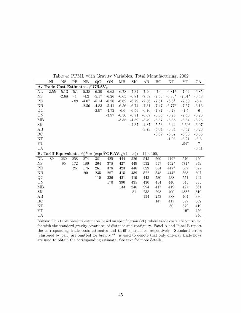
Table 4: PPML with Gravity Variables, Total Manufacturing, 2002NL NS PE NB QC ON MB SK AB BC NT YT CA

A. Trade Cost Estimates, β′GRAVij

NL -2.55 -5.13 -5.1 -5.28 -6.29 -6.63 -6.78 -7.34 -7.46 -7.6 -6.81* -7.64 -6.85NS -2.68 -4 -4.2 -5.17 -6.26 -6.65 -6.81 -7.38 -7.53 -6.83* -7.61* -6.48PE -.89 -4.07 -5.14 -6.26 -6.62 -6.79 -7.36 -7.51 -6.8* -7.59 -6.4NB -2.56 -4.83 -5.41 -6.56 -6.74 -7.31 -7.47 -6.77* -7.57 -6.13QC -2.97 -4.72 -6.6 -6.59 -6.76 -7.37 -6.73 -7.5 -6ON -3.97 -6.36 -6.71 -6.67 -6.85 -6.75 -7.46 -6.26MB -3.38 -4.89 -5.49 -6.57 -6.58 -6.64 -6.26SK -2.37 -4.87 -5.53 -6.44 -6.69* -6.07AB -3.73 -5.04 -6.34 -6.47 -6.26BC -3.62 -6.57 -6.33 -6.56NT -1.05 -6.21 -6.6YT .84* -7CA -6.41B. Tariff Equivalents, τFEij = (exp(β′GRAVij/(1− σ))− 1)× 100,NL 89 260 258 274 381 425 444 526 545 569 449* 576 420NS 95 172 186 264 378 427 449 532 557 452* 571* 349PE 25 176 261 378 423 446 529 554 447* 567 327NB 90 235 287 415 439 522 548 444* 563 307QC 110 226 421 419 443 530 438 551 292ON 170 390 435 430 454 440 545 335MB 133 240 294 417 419 427 361SK 81 238 298 400 433* 319AB 154 253 388 404 336BC 147 417 387 362NT 30 372 419YT -19* 456CA 346Notes: This table presents estimates based on specification (21), where trade costs are controlledfor with the standard gravity covariates of distance and contiguity. Panel A and Panel B reportthe corresponding trade costs estimates and tariff-equivalents, respectively. Standard errors(clustered by pair) are omitted for brevity.“*” is used to denote that only one-way trade flowsare used to obtain the corresponding estimate. See text for more details.

45

Table 5: Gravity Trade Costs, CA Mnufacturing 2002

(1) (2) (3) (4)BENCHMARK TEST CONSTRAINT TRANSLOG

ln(tGRAVij )1−σ 1.141 0.965 0.997 0.959(0.090)** (0.035)** (0.036)** (0.039)**

ln(tGRAVii )1−σ -0.607 -0.487 -0.473(0.035)** (0.023)** (0.213)*

ln(tGRAVjj )1−σ -0.621 -0.513 -0.545(0.032)** (0.023)** (0.191)**

ln(tGRAVii )2(1−σ) 0.003(0.021)

ln(tGRAVjj )2(1−σ) -0.009(0.018)

ln(tGRAVii )1−σ × ln(tGRAVjj )1−σ 0.035(0.036)

CONST 4.259 -1.059 -0.077 -0.710(0.596)** (0.283)** (0.235) (0.767)

N 126 126 126 126R2 0.475 0.938 0.939

Notes: This table reports results from neutrality tests based on specification (22). The regression in Column(1) includes only bilateral trade costs ln

(tGRAVij

). Column (2) adds intra-regional trade costs ln

(tGRAVii

)and ln

(tGRAVjj

). Column (3) restricts the sum of the coefficients on ln

(tGRAVii

)and ln

(tGRAVjj

)to equal

-1. Lastly, Column (4) tests the translog specification be including the squared terms of ln(tGRAVii

)and

ln(tGRAVjj

)and their interaction. Bootstrapped standard errors in parentheses. See text for more details.

+ p < 0.10, * p < .05, ** p < .01

Table 6: UTB, Total Manufacturing, 2002, Cobb-Douglas SpecificationNS PE NB QC ON MB SK AB BC NT YT

NL -.07 -.27 -.07 .01 .135 .07 -.02 .135 .13 -.19 -.375NS -.295 -.1 -.02 .135 .08 -.03 .15 .14 -.18 -.37PE -.305 -.22 -.065 -.125 -.23 -.055 -.065 -.38 -.57NB -.04 .09 .065 -.04 .13 .125 -.19 -.375QC .115 .11 0 .16 .17 -.145 -.335ON .22 .115 .27 .26 -.035 -.225MB -.015 .16 .19 -.105 -.315SK .025 .035 -.225 -.44AB .17 -.075 -.285BC -.08 -.305NT -.6Notes: This table reports the UTBs constructed based on equation(25). See text for more details.

46

Table 7: CTB Indexes, Total Manufacturing, 2002NL NS PE NB QC ON MB SK AB BC NT YT CA

A. CTB Levels, 2002NL 1141 44.3 72 30.2 4.8 2 3.8 2.9 2.8 2.8 23.1 3.9 4.1NS 178 579.7 248.5 117.5 12.7 6.1 9.5 7.8 8.7 8.1 153 17.1 11.4PE 149.7 128.5 4371.1 137.1 14.1 4.2 8.3 6.7 4.7 5.9 30.6 17.3 11.5NB 104.3 100.9 227.7 440 16.5 7 6.6 6.8 5.6 4.7 38.5 21.3 11.3QC 22.7 14.9 31.9 22.5 65.6 7.1 10 7.8 7.9 6.5 41.9 13.9 7.9ON 15 11.6 15.3 15.4 11.5 19.8 7.1 8.8 10.3 6.9 19.7 14.8 10.1MB 18.1 11.3 19.2 9.1 10.1 4.5 251.6 74.7 40 16.9 68.6 37.5 11.5SK 12.2 8.2 13.8 8.4 7 4.9 66.2 493.5 66.7 22.6 42 18.9 14.2AB 11.2 8.7 9.2 6.5 6.7 5.4 33.5 63 181 38 101.4 56.1 11.4BC 7.2 5.2 7.2 3.5 3.5 2.3 9 13.6 24.2 127.2 42.1 74.7 5.2NT 3.2 .9 5.1 3.5 9 5.9 16927.4 109.1 2.7YT 1 .7 4.9 10.3 106.9 68851.5 2.3B. Relative Sellers’ Incidence (CTBij/CTBii)1/(1−σ), 2002NL 1 2.3 2 2.5 3.9 4.9 4.2 4.5 4.5 4.5 2.7 4.1 4.1NS 1.3 1 1.2 1.5 2.6 3.1 2.8 2.9 2.9 2.9 1.4 2.4 2.7PE 2.3 2.4 1 2.4 4.2 5.7 4.8 5 5.5 5.2 3.5 4 4.4NB 1.4 1.4 1.2 1 2.3 2.8 2.9 2.8 3 3.1 1.8 2.1 2.5QC 1.3 1.4 1.2 1.3 1 1.7 1.6 1.7 1.7 1.8 1.1 1.5 1.7ON 1.1 1.1 1.1 1.1 1.1 1 1.3 1.2 1.2 1.3 1 1.1 1.2MB 1.9 2.2 1.9 2.3 2.2 2.7 1 1.4 1.6 2 1.4 1.6 2.2SK 2.5 2.8 2.4 2.8 2.9 3.2 1.7 1 1.6 2.2 1.9 2.3 2.4AB 2 2.1 2.1 2.3 2.3 2.4 1.5 1.3 1 1.5 1.2 1.3 2BC 2 2.2 2 2.5 2.5 2.7 1.9 1.7 1.5 1 1.3 1.1 2.2NT 8.5 11.6 7.6 8.3 6.6 7.3 1 3.5 8.9YT 16 17.8 10.9 9.1 5 1 13.2C. (CTBFE − CTBGRAV )/CTBFE

NL .2 24.9 21.3 12.1 20.4 -7.8 -80.9 -26.2 -26.9 3.1 -82.2 -256.2 0NS 3 -.7 -19.3 -15.3 -60.7 12.3 -42.3 -37 22.7 36.7 53 -44.6 8.7PE 10.1 -5.5 .1 14.2 -13 2.6 -26.2 -22.2 -9 32.8 -84.4 -10 7.1NB -2.2 -3.9 12.7 .3 -25.3 -29.1 -61.9 -20.5 8 17.3 -42.4 12.6 8.8QC 2.2 -53.1 -21.6 -32.4 -.3 -43.5 41.7 29.8 35.4 61.7 21.9 18.2 6.2ON -8.7 31.5 14 -11.9 -17.8 .8 -7.6 43 43.5 37.5 -69 16.7 8.9MB -50.3 8.3 8.2 -15.7 60.6 11.3 -.3 20.3 9.1 35.3 -10 -42.3 9.3SK 3.3 18.6 18 20.5 56.2 56.7 26.5 -.1 23.3 -4.9 -58.1 -104.9 11.8AB -20.3 43.2 9.5 25 50.1 46.9 -3.8 5.1 .2 -31.3 6.3 -11.8 9.4BC -13 42.8 31.3 17 63.6 27.7 9.1 -59.7 -61.5 .9 -25.3 32.9 3NT -11.6 -194.3 -132.5 -262 -73.4 -88.4 0 23.6 -6.2YT -30.7 -62.1 -131.3 -12.9 14.6 0 -10.9Notes: This table presents estimates of the Constructed Trade Bias index, as defined in specification(18). Panel A reports CTBs in levels for 2002, while Panel B reports Constructed Inter-provincial Biasvalues (as defined in (5)). Panel C reports percentage differences between the CTB indexes constructedusing the fixed effects method (13), and the standard gravity variables approach, (21). See text formore details.

47

Table 8: CTB Percentage Changes, Total Manufacturing, 1997-2007NL NS PE NB QC ON MB SK AB BC NT YT CA

NL -3.7 15.4 -7 6.4 15 23.8 17 -4.3 5.1 11.4 2.2 104.2 14.3NS 15.8 -12.8 -11.3 1.5 9.6 18 11.6 -8.8 .2 6.1 -2.6 94.7 7PE 45.6 38.3 -11.6 27.6 37.8 48.3 40.3 14.7 26 33.5 22.5 144.8 32.7NB 50.2 42.6 15 4.2 42.1 52.9 44.6 18.2 29.9 37.6 26.3 152.4 42.6QC 26.2 19.9 -3.4 10.5 -5.4 28.5 21.5 -.6 9.1 15.6 6.1 112.1 22.4ON 1.1 -4 -22.6 -11.5 -4.4 -18.4 -2.7 -20.4 -12.6 -7.4 -15 69.9 -7.8MB 2 -3.2 -21.9 -10.7 -3.5 3.8 -22.2 -19.7 -11.8 -6.6 -14.3 71.3 -.8SK 49.4 41.9 14.4 30.9 41.4 52.2 43.9 -6.7 29.2 37 25.7 151.2 53.4AB 9.7 4.2 -16 -3.9 3.8 11.8 5.7 -13.6 -24.8 .6 -7.7 84.4 5.8BC 40.4 33.4 7.5 23 32.9 43 35.3 10.6 21.4 2 18.1 136 43.7NT -45.4 -41.2 -44.4 -54.5 -50.1 -47.1 -61.5 -3 -41.3YT -85.1 -84 -86.4 -85.6 -86.8 -79.1 -83.8Notes: This table reports CTB percentage changes over the period 1997-2007.

Table 9: Intra-provincial costs and CTBs(1) (2)

CTBC(i) (γii = 0) CTBC(i) (γii 6= 0)NL 9 11.6NS 17.8 22.5PE 19.1 20.5NB 15.1 19.4QC 18.2 19.6ON 31.1 15.1MB 12.5 16.4SK 16.6 19.1AB 28.6 23.9BC 19.9 16.9NT 28.1 30.9YT 32.7 32.6Notes: This table reports CTBs whichare constructed without intra-provincialtrade costs (column 1) and with intra-provincial trade costs (column 2).

48

Table 10: Gravity Residuals as Percent of CTB, Total Manufacturing, 2002NL NS PE NB QC ON MB SK AB BC NT YT CA

NL -1.5 130.3 -13.5 -65.7 -20.9 -45.2 -55.2 10.6 -36.3 -77 -18.5 1.5 -9.8NS 16 -2.5 15 -1.1 1.6 8.4 -18.8 61.4 10.4 -44.8 -39.2 52.6 2.6PE -14 -26.1 .1 1.9 -4.4 38.4 84.6 -43.4 7.9 -48.6 46 183.3 0NB 8.1 -10.2 -11.5 4.3 43.9 -53.4 -29.5 -45 -42.3 -43.6 -.1 71.1 -13.3QC .7 -1.6 15.9 -32.4 .8 14.2 14.6 12.3 8.7 -4.4 -7.7 7.5 8.9ON 3.8 -6.6 -20.2 16.6 -.4 .7 -31.3 17.9 1 -2.5 -15.1 29.4 0MB -20.9 3.7 3.5 21.2 -16.4 35 -4.7 -.2 .2 -8.4 11.9 15.9 3.5SK 36.7 24 -30.8 16.7 -11.2 8.1 17.4 -1.8 -2.8 14 -6 -25.3 4.2AB -2 -7.3 -21.8 6.2 -14.1 -12.1 7.1 8.4 -.8 -19.8 -13.6 34.3 -10.5BC 15.7 -2.4 22.8 13.8 -3 9.4 27.7 31 21.3 -3.7 -24.1 -.3 13.5NT -68.7 -3.6 -100 -55.6 -18.7 12.9 .7 -100 -25.9YT -51.6 -47.9 23.5 204 -41.5 0 78.3Notes: This table reports estimates of the Gravity Residuals as a percentage of theCTB index for 2002. See text for more details.

49