intrinsic and rational speculative bubbles in the u.s ... · market over the last 50 years. in our...
TRANSCRIPT
J R E R � V o l . 3 5 � N o . 2 – 2 0 1 3
I n t r i n s i c a n d R a t i o n a l S p e c u l a t i v eB u b b l e s i n t h e U . S . H o u s i n g M a r k e t :1 9 6 0 – 2 0 1 1
A u t h o r s Ogonna Nnej i , Chris Brooks, and
Charles Ward
A b s t r a c t : This paper examines the dynamics of the residential propertymarket in the United States between 1960 and 2011. Given thecyclicality and apparent overvaluation of the market over thisperiod, we determine whether deviations of real estate pricesfrom their fundamentals were caused by the existence of twogenres of bubbles: intrinsic bubbles and rational speculativebubbles. We find evidence of an intrinsic bubble in the marketpre-2000, implying that overreaction to changes in rentscontributed to the overvaluation of real estate prices. However,using a regime-switching model, we find evidence of periodicallycollapsing rational bubbles in the post-2000 market.
Over the last decade, residential property prices in the United States have attractedmuch attention from the media. According to the house price index provided bythe Federal Housing and Finance Agency, nominal house prices rose by 61%between 1999 and 2009. This sharp rise has attracted the attention of academicresearchers, some of whom are interested in establishing whether this increase inproperty prices is due to the existence of a bubble in the market.
An extended deviation of house prices from their fundamental values could bedetrimental to the economy if it leads to a subsequent collapse in the housingmarket; research shows that homes are the major assets in household portfolios(Englund, Hwang, and Quigley, 2002). Changes in housing-based wealth areshown to be more important in their effect on the economy than changes in wealthcaused by movements in stock prices (Helbling and Terrones, 2003; Rapach andStrauss, 2006). Pavlidis, Paya, Peel, and Spiru (2009) find that bubbles in thehousing market account for a significant share of changes to consumerexpenditure. Hence, if house prices are not monitored closely, a crash could havea large adverse impact on the economy. The study of housing bubbles is thereforean important contribution to the literature on future economic development.
Speculative bubbles are certainly not new phenomena, with bubbles identified incommodity and financial markets at least back to the seventeenth century in the
1 2 2 � N n e j i , B r o o k s , a n d W a r d
Netherlands (Garber, 1990). Researchers have investigated the possible presenceof speculative bubbles in numerous asset classes and several new models havebeen proposed. An important class of such models is based on rational speculativebubbles. These arise when the expectation of the future price of an asset has anabnormally important influence on the asset’s current valuation, which couldstimulate demand and thus lead to a deviation of asset prices from theirfundamentals. Thus rational bubbles are influenced by extraneous events that areindependent of fundamentals. In the context of a rational bubble, investors arejustified in paying ever-higher prices for the asset because they are compensatedfor the risk that the bubble will collapse by increasing returns. On the other hand,intrinsic bubbles, another genre of speculative bubbles, are driven solely byoverreaction to changes in fundamentals (see the following section for moredetails).
The contributions of this paper to the literature on housing bubbles are twofold.Firstly, it is the first to simultaneously examine whether intrinsic and rationalspeculative bubbles exist in the U.S. residential real estate market. The secondcontribution is that we test whether or not changes in rents predict futureinvestment returns on residential properties during periods in which intrinsicbubbles are present and during periods of no intrinsic bubbles. This research isthe first of its kind as no previous paper has accounted for the presence of bubbleswhen testing for the predictive power of rents.
� T h e E x i s t i n g L i t e r a t u r e
Blanchard and Watson (1982) introduce a model of rational speculative bubblesthat can capture the rise and subsequent rapid fall of prices relative tofundamentals, albeit with two key disadvantages. The first is the implicitsuggestion that bubbles will grow exponentially and can never be negative, asrational investors would never expect the future price of a stock to fall below zero.The second is that the model assumes two states of nature, with the first statebeing one in which the bubble survives and the second state representing thebubble collapse. It follows that once the bubble pops, it would never be able toregenerate. Diba and Grossman (1988) further develop this theory and additionallyconclude that for a rational bubble to exist, stock prices’ successive differenceswill be nonstationary.
However, papers by van Norden and Schaller (hereafter vNS, 1993, 1999) and byBrooks and Katsaris (2005a, 2005b) dispute this approach, arguing that it istheoretically unjustifiable and leads to empirically implausible results. vNS (1993)propose a model in which bubbles could regenerate after a collapse, as can beseen in observed successions of rallies and crashes in stock markets.
Froot and Obstfeld (1991) introduce a different class of bubbles termed ‘‘intrinsicbubbles.’’ Intrinsic bubbles, unlike rational speculative bubbles, are influencedsolely by fundamentals such as dividends (in the case of stock prices), albeit
I n t r i n s i c a n d R a t i o n a l S p e c u l a t i v e B u b b l e s � 1 2 3
J R E R � V o l . 3 5 � N o . 2 – 2 0 1 3
in a nonlinear way. Intrinsic bubbles revert back to their fundamental valuesperiodically. This class of bubbles is also rational and relies on the self-fulfillingexpectations of market participants. The difference between intrinsic bubbles andstandard rational speculative bubbles is that in the former case, deviations arecaused by a nonlinear relationship between fundamentals and prices rather thanextraneous factors that would not normally be expected to influence the value ofthe asset. Froot and Obstfeld show that intrinsic bubbles closely capture theoverreaction of stock prices to changes in dividends. Ma and Kanas (2004) providefurther evidence supporting the model for intrinsic bubbles by examining thenonlinear cointegration between stock prices and dividends.
There have been a number of studies designed to test for the existence of bubblesin real estate prices, stimulated by the persistent rising trend in house prices thatappeared to have been unrelated to economic variables, such as construction costs,disposable incomes, and unemployment. Bjorklund and Soderberg (1999) examinethe possibility that house prices in Sweden are driven by the presence ofspeculative bubbles. They observe the dynamics of the Gross Income Multiplier(GIM), asserting that only the presence of a speculative bubble can cause the GIMto have a different trend from the real estate cycle. Kim and Lee (2000) adopt acointegration approach to test for the presence of a bubble in the Korean propertymarket. They infer the presence of a bubble in the market on the grounds that, inperiods when the bubble is expanding, the variables are not cointegrated andtherefore that there is no observable long-run equilibrium relationship betweenthe variables. Similarly, Mikhed and Zecik (2009) test for bubbles in 23metropolitan statistical areas (MSAs) in the U.S. between 1975 and 2006 usingunit root tests. They derive the fundamental value of real estate using the presentvalue of future rents. They find evidence of bubbles because fundamental valueswere stationary while observed prices were non-stationary.
A more econometrically robust test for bubbles is performed by Roche (2001).Using a regime-switching model, he tests for and finds the presence of periodicallycollapsing rational bubbles in the Dublin residential property market. Morerecently, Lai and van Order (2010) test for housing bubbles in the U.S. byexamining the momentum of house price growth in several MSAs. They findmomentum to have increased significantly after 1999, which led to the inceptionof a bubble.
The only notable test for bubbles in the real estate market that is not based on aneconometric approach is conducted by Zhou and Sornette (2006). They apply theirtest to the housing market of different states in the U.S. Using an ‘‘econophysics’’method, their approach examines the speed at which house prices grew. A fasterthan exponential growth in house prices could be concluded to indicate theexistence of a bubble. They find that 22 states exhibited evidence of bubbles.Another state-level analysis is conducted by Abraham and Hendershott (1996),who observe bubbles in U.S. Northeast and West coastal cities. Although muchof the research is based on the residential market, bubbles are also observed byHendershott (2000) to be present in the office market in Sydney.
1 2 4 � N n e j i , B r o o k s , a n d W a r d
Several other relevant papers have tested for bubbles in the U.S. real estate market,including Giliberto (1992), Case and Shiller (2004), Goodman and Thibodeau(2008), and Wheaton and Nechayev (2008). There is also evidence of speculativebubbles in real estate investment trusts (REITs) (e.g., Brooks, Katsaris, McGough,and Tsolacos, 2001; Payne and Waters, 2005, 2007; and Jirasakuldech, Campbell,and Knight, 2006).
All of the above studies in real estate address the existence of rational bubbles.However, existing evidence concerning the presence of intrinsic bubbles is verysparse. Black, Fraser, and Hoesli (2006) and Fraser, Hoesli, and McAlevey (2008)represent the only studies that test for the presence of intrinsic bubbles in the realestate market, focusing on the United Kingdom and New Zealand propertymarkets. The two papers apply the same methodology in calculating thefundamental values. They measure fundamentals based on the present value of theexpected future disposable income of households. By testing for the presence ofintrinsic bubbles in the two countries, they investigate whether deviations of houseprices from their fundamentals are caused by an overreaction of households tochanges in the expected future values of their disposable incomes. Both papersfind intrinsic bubbles to be present only in the U.K., while deviations fromfundamentals in New Zealand appear to have been influenced by price dynamicsalone and therefore classified as a rational but not intrinsic bubble.
The bubbles identified by the above literature to be present in the housing marketmay have contributed to the ambiguous results of an entirely separate strand ofreal estate research that sought to identify whether price changes could bepredicted by rents. Mankiw and Weil (1989) find the relationship between futureprice changes and the rent-price ratio to be statistically insignificant. Even withthe use of an error-correction model, Gallin (2004) shows that the power of therent-price ratio for predicting future house prices is inconclusive. Hatzvi and Otto(2008) also find no concrete evidence to suggest that an increase in real rentswould strongly influence variations in the prices of residential property. Referringto the U.K. housing market, Baddeley (2005) concludes that modeling the marketis more efficient when factors that might destabilize it are accounted for in theanalysis. Such factors might include the presence of bubbles, herding, and frenzies.Building on Baddeley’s conclusion, we aim to establish whether or not there havebeen intrinsic or rational speculative bubbles in the U.S. housing market and weexamine the role of fundamental factors in forecasting future price changes differsbetween bubble and nonbubble periods.
In this paper, our objective is to understand the price dynamics of the U.S. housingmarket over the last 50 years. In our analysis, we test to see whether house pricesdiffer from their fundamental values, and, if so, whether such deviations are drivenby an overreaction of house prices to changes in rents (i.e., whether there is anintrinsic bubble or not). Although Black, Fraser, and Hoesli (2006) and Fraser,Hoesli, and McAlevey (2008) have, as reported above, tested whether deviationsof house prices from their fundamental values were due to an overreaction tochanges in fundamentals in the U.K. and New Zealand, this is the first paper tohave addressed the issue in the U.S. market.
I n t r i n s i c a n d R a t i o n a l S p e c u l a t i v e B u b b l e s � 1 2 5
J R E R � V o l . 3 5 � N o . 2 – 2 0 1 3
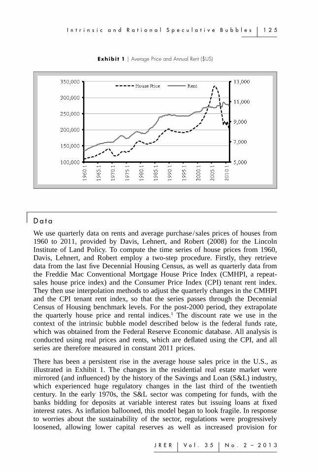
Exhibi t 1 � Average Price and Annual Rent ($US)
� D a t a
We use quarterly data on rents and average purchase/sales prices of houses from1960 to 2011, provided by Davis, Lehnert, and Robert (2008) for the LincolnInstitute of Land Policy. To compute the time series of house prices from 1960,Davis, Lehnert, and Robert employ a two-step procedure. Firstly, they retrievedata from the last five Decennial Housing Census, as well as quarterly data fromthe Freddie Mac Conventional Mortgage House Price Index (CMHPI, a repeat-sales house price index) and the Consumer Price Index (CPI) tenant rent index.They then use interpolation methods to adjust the quarterly changes in the CMHPIand the CPI tenant rent index, so that the series passes through the DecennialCensus of Housing benchmark levels. For the post-2000 period, they extrapolatethe quarterly house price and rental indices.1 The discount rate we use in thecontext of the intrinsic bubble model described below is the federal funds rate,which was obtained from the Federal Reserve Economic database. All analysis isconducted using real prices and rents, which are deflated using the CPI, and allseries are therefore measured in constant 2011 prices.
There has been a persistent rise in the average house sales price in the U.S., asillustrated in Exhibit 1. The changes in the residential real estate market weremirrored (and influenced) by the history of the Savings and Loan (S&L) industry,which experienced huge regulatory changes in the last third of the twentiethcentury. In the early 1970s, the S&L sector was competing for funds, with thebanks bidding for deposits at variable interest rates but issuing loans at fixedinterest rates. As inflation ballooned, this model began to look fragile. In responseto worries about the sustainability of the sector, regulations were progressivelyloosened, allowing lower capital reserves as well as increased provision for
1 2 6 � N n e j i , B r o o k s , a n d W a r d
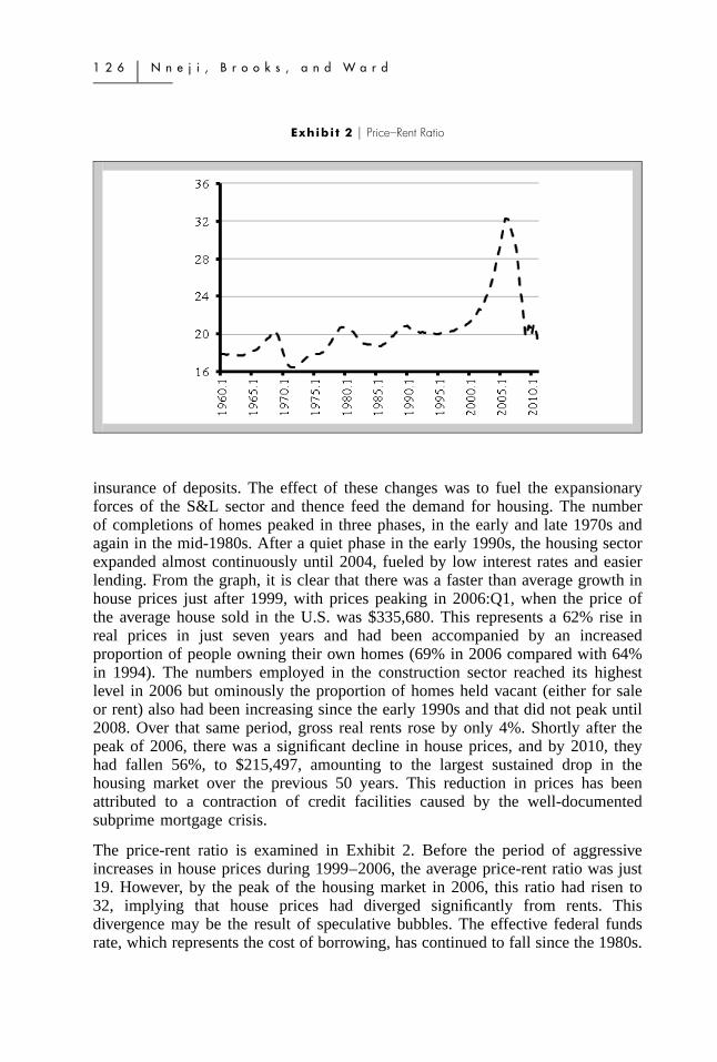
Exhibi t 2 � Price–Rent Ratio
insurance of deposits. The effect of these changes was to fuel the expansionaryforces of the S&L sector and thence feed the demand for housing. The numberof completions of homes peaked in three phases, in the early and late 1970s andagain in the mid-1980s. After a quiet phase in the early 1990s, the housing sectorexpanded almost continuously until 2004, fueled by low interest rates and easierlending. From the graph, it is clear that there was a faster than average growth inhouse prices just after 1999, with prices peaking in 2006:Q1, when the price ofthe average house sold in the U.S. was $335,680. This represents a 62% rise inreal prices in just seven years and had been accompanied by an increasedproportion of people owning their own homes (69% in 2006 compared with 64%in 1994). The numbers employed in the construction sector reached its highestlevel in 2006 but ominously the proportion of homes held vacant (either for saleor rent) also had been increasing since the early 1990s and that did not peak until2008. Over that same period, gross real rents rose by only 4%. Shortly after thepeak of 2006, there was a significant decline in house prices, and by 2010, theyhad fallen 56%, to $215,497, amounting to the largest sustained drop in thehousing market over the previous 50 years. This reduction in prices has beenattributed to a contraction of credit facilities caused by the well-documentedsubprime mortgage crisis.
The price-rent ratio is examined in Exhibit 2. Before the period of aggressiveincreases in house prices during 1999–2006, the average price-rent ratio was just19. However, by the peak of the housing market in 2006, this ratio had risen to32, implying that house prices had diverged significantly from rents. Thisdivergence may be the result of speculative bubbles. The effective federal fundsrate, which represents the cost of borrowing, has continued to fall since the 1980s.

I n t r i n s i c a n d R a t i o n a l S p e c u l a t i v e B u b b l e s � 1 2 7
J R E R � V o l . 3 5 � N o . 2 – 2 0 1 3
Exhibi t 3 � Federal Funds Rate
Exhibit 3 shows that, as of 2008, the rate was around 2% compared to 16% in1981. It has been suggested that these persistent cuts in interest rates contributedto the sharp rise in house prices over this period, although subsequently interestrates remained at extremely low levels even as prices collapsed.
� M e t h o d o l o g y
Examining the price-rent ratio provides information on when the trend in pricesdeparts from the growth trend in rents, which could imply the presence of a bubble(Mikhed and Zemcik, 2009). The underlying assumption is that the asset priceseries at some point starts to incorporate a bubble and, at a later point, the bubblebursts. But from casual observation, bubbles are not equally likely to occur at anypoint in time; rather, they usually occur when the market is in a state predisposedto a bubble. We take the view that bubbles are more likely to occur when themarket is more volatile. In order to work within this view, we choose to modelthe market using a Markov regime-switching approach in which the market maybe classified into two regimes: low return/high volatility and high return/lowvolatility. We test for regime switching in the price-rent ratio series. Applying aMarkov regime-switching methodology, we use the probabilities generated todetermine when the price-rent ratio series switches regimes. Using the computedprobabilities from the Markov regime-switching model, the data are then split intotwo sub-periods. We separately test for the presence of intrinsic and periodicallypartially collapsing rational speculative bubbles in the housing market in both sub-periods.2
1 2 8 � N n e j i , B r o o k s , a n d W a r d
L o c a t i n g R e g i m e s i n t h e P r i c e - R e n t R a t i o S e r i e s
In order to determine the sub-periods, we assume that the price-rent ratio, (P /R),can be modeled by the following process:
P P� a � � � , (1)� � � � tR Rt t�1
where:
2� � i.i.d(0,� ) (2)t
and a is constant drift term.
This means that the price-rent ratio in the current period is equivalent to theprevious period’s price-rent ratio plus a constant representing the drift of theprocess. Re-arranging (1):
P P� � a � � . (3)� � � � tR Rt t�1
Applying the Markov regime-switching methodology to (3), we obtain (4):
P P� � a (1 � s ) � a s � (� (1 � s ) � � s )� .� � � � 0 t 1 t 0 t 1 t tR Rt t�1
(4)
This is now a Markov-switching model,3 with st being a latent state variable thatis assumed to follow a first-order Markov chain with constant transitionprobabilities, which we define as:
Pr (s � 1 �s � 1) � p (5a)t t�1
Pr (s � 0 �s � 1) � 1 � p (5b)t t�1
Pr (s � 0 �s � 0) � q (5c)t t�1
Pr (s � 1 �s � 0) � 1 � q. (5d)t t�1
I n t r i n s i c a n d R a t i o n a l S p e c u l a t i v e B u b b l e s � 1 2 9
J R E R � V o l . 3 5 � N o . 2 – 2 0 1 3
This state variable can be either zero or one, representing the two possible regimesof the price-rent ratio series. In this case, the probability of being in one regimeis influenced only by the state that prevailed during the previous period.
By implementing this Markov regime-switching random walk with a drift model,we could then use the probabilities generated to determine the period in whichthe price-rent ratio switches to a separate regime with different mean and variance.Hence, we split our data into sub-periods based on these probabilities and applythe intrinsic bubble test to the sub-periods.
A n I n t r i n s i c B u b b l e Te s t
As described above, Froot and Obstfeld (1991) introduce the concept of intrinsicbubbles which, unlike rational speculative bubbles, are deviations of observedprices from the fundamental price driven by fundamentals in a nonlinear fashion.In contrast with previous studies on intrinsic bubble models that use disposableincome as the key fundamental driver of house prices, we use rents as ourfundamental measure. The main reason we opt to use rents rather than disposableincome is that they directly represent the consumption market for physical space.A shortfall in the supply of space will lead to an increase in rents. But a bubblein the sense of financial market bubbles should not affect the nominal level ofrents since the rent is essentially the spot price for immediate space occupationand is not itself an investible asset. From the real estate investor’s viewpoint, rentis analogous in cash flow terms to dividends for equity market investors. Rentsprovide better fundamental measures than disposable incomes in countries witheasy access to credit facilities, like the U.S. (historically at least), where the abilityof individuals to acquire mortgages did not depend solely on their disposableincomes. In those countries, changes in disposable incomes have not necessarilybeen associated with fundamental changes in the demand for housing.Furthermore, several studies have shown that rents are fundamental driversincluding Campbell, Davis, Gallin, and Martin (2009), who show that variationsin housing valuations are due to growth in rental values, the interest rate, andhousing premia changes. There is no mention of disposable incomes.
To carry out the test for intrinsic bubbles in the U.S. housing market, we followthe Froot and Obstfeld (1991) approach, but replace dividends with rents. Hencethe present value relationship describing house prices is given by:
�pv �ir(s�t�1)P � e E (R ), (6)�t t t s
s�t
where is the present value of the house price in period t, ir is the constantpvPt
interest rate, R is the gross rents value, and E is the expectation of the marketgiven information at the start of period t. A standard bubble model is given as:
1 3 0 � N n e j i , B r o o k s , a n d W a r d
pvP � P � B (7)t t t
where:
�irB � e E (B ). (8)t t t�1
The actual price of a house is given by Pt while the bubble term, Bt, is thedifference between the actual price and the fundamental value. However, theintrinsic bubble model considers bubbles that are generated by a nonlinear functionof rents. Hence the intrinsic bubble is a function of rents satisfying (8):
�B (R ) � cR , (9)t t t
where c and � are constants explained below.4
The model also assumes that log rents are generated as a martingale. Hence, theprocess for log rents, rt, must follow a random walk with a drift �:
r � � � r � � (10)t�1 t t�1
where:
2� � N(0,� ).t�1
From (6), the house price’s present value ought to be proportional to rents if therent during period t is known:
pvP � �R (11)t t
where:
2ir ��� /2� � (e � e ). (12)
I n t r i n s i c a n d R a t i o n a l S p e c u l a t i v e B u b b l e s � 1 3 1
J R E R � V o l . 3 5 � N o . 2 – 2 0 1 3
The sum in (6) is assumed to converge, thereby implying that ir must be greaterthan � � �2/2. Also, this condition is required to ensure that we do not yieldnegative present values. Therefore, if a bubble is present, the observed house price,Pt, can be thought of as the sum of and Bt(Rt):pvPt
pv �P(R ) � P � B (R ) � �R � cR , (13)t t t t t t
where c is an arbitrary constant and � is the positive root of (14),5 which areobtained from the inequality condition ir � � � �2/2:
2� 2� � �� � ir � 0. (14)2
Based on (14), the inequality ir � �2/2 �2 � �� is used to indicate that � mustbe greater than one at all times, and it is this explosive nonlinearity that allowshouse prices to overreact to changes in rents. Like Froot and Obstfeld (1991), wethen divide (13) by Rt due to the presence of collinearity,6 using:
Pt ��1� � � cR � � (15)t tRt
to test for the presence of intrinsic bubbles in the housing market. The nullhypothesis in this case is that c � 0, implying that there is no intrinsic bubblepresent.
A R a t i o n a l S p e c u l a t i v e B u b b l e Te s t
To determine whether real estate prices between 1960 and 2011 were insteaddriven by extraneous events that are independent of fundamentals, we employ thevNS (1993, 1999) model. Note that this approach to testing for rational speculativebubbles was also used by Roche (2001) to test for bubbles in the Irish housingmarket. This model tests for the presence of periodically collapsing rationalspeculative bubbles in an asset. In order to fully understand the vNS specification,it is important to briefly discuss the Blanchard and Watson (1982) model.According to their model, prices are decomposed into two parts: the fundamentalvalue and the bubble component, as seen in (7). In this model, the bubblecomponent grows at an exponential rate and cannot be negative in value, implyingthat observed prices must always equal or exceed the fundamental value. Themodel also assumes that two bubble states exist, the first being one where the
1 3 2 � N n e j i , B r o o k s , a n d W a r d
bubble survives (S) and the other being a state where the bubble collapses (C),implying the bubble process to be:
(1 � ir)E (B �S) � B with probability qt t�1 tq
E (B �C) � 0 with probability 1 � q (16)t t�1
where the probabilities of the bubble surviving and collapsing are q and 1 � q,respectively.
The process in (16) implies that the bubble component in period t � 1 is expectedto grow at a faster rate than the real rate of return if the bubble does not collapse,thus compensating the investor for risk taking.7 However, in the event of thebubble collapsing, its value immediately falls to zero and the observed price wouldequal the fundamental value. This model also concludes that the bubble cannotregenerate once it collapses. Therefore, these assumptions are not realistic as therehave been significant episodes of bubble crashes and regenerations.
The vNS approach is an extension of the Blanchard and Watson (1982) model,eliminating the assumption of a bubble being unable to regenerate following acollapse. vNS also allow the probability of a bubble collapsing to depend on itssize relative to the asset price (bt � Bt /Pt), i.e., an increase in the bubble relativeto the asset price increases the probability of a collapse. Lastly, they allow for thegradual collapse of speculative bubbles, unlike Blanchard and Watson’s model,which assumes the value of a bubble to equal zero once it has collapsed. Therefore,the vNS stochastic bubble process is given as:
(1 � ir) 1 � q(b )tE (B �S) � B � u(b )Pt t�1 t t tq(b ) q(b )t t
with probability q(b )t
E (B �C) � u(b )P with probability 1 � q(b ) (17)t t�1 t t t
where u(bt) is a continuous and everywhere differentiable function:
�u(b )t0 1. (18)�bt
I n t r i n s i c a n d R a t i o n a l S p e c u l a t i v e B u b b l e s � 1 3 3
J R E R � V o l . 3 5 � N o . 2 – 2 0 1 3
Here, the expected size of the bubble in the collapsing regime does notimmediately reduce to zero. Instead, it decreases gradually. Note that theprobabilities q are now represented as q(bt), implying that it is dependent on thesize of the bubble relative to prices. To calculate the fundamental value of housing,we use the average price-rent ratio multiplied by the rent during the selected timeperiod:
PƒP � R . (19)t tR
Therefore, the nonfundamental or rational speculative bubble component of thestock is given by simply subtracting the actual price of the stock from itsfundamental component (i.e., the proportion of observed price that is not explainedby rents), as shown in (20):
PB � P � R . (20)t t tR
Under this bubble specification model, vNS note that returns to a ‘‘bubbly’’ assetought to be state dependent such that periodically collapsing bubbles induceregime switches in asset returns:
sW � � b � ut�1 s,0 s,1 t s,t�1
cW � � b � ut�1 c,0 c,1 t c,t�1
q(b ) � �( � �b �) (21)t q,0 q,1 t
where W represents the return on investing in real estate, the unexpected returnsin the collapsing and surviving regimes are represented by uc,t�1 and us,t�1
respectively, and they have constant variance and zero mean. � represents thestandard normal cumulative distribution function and so �(q,0) is the averageprobability of being in the surviving regime. On the other hand, q,1 measureshow the probability of being in the surviving regime changes with respect to theabsolute bubble size as a proportion of the actual price.
To estimate the parameters in (21), we maximize the following log-likelihoodfunction (l):
1 3 4 � N n e j i , B r o o k s , a n d W a r d
W � � bt�1 S,0 S,1 t� � �T �S
l (W ��) � ln q(b )� �t�1 t �t�1 S
W � � bt�1 C,0 C,1 t� � ��C� (1 � q(b )) . (22)�t �C
Here, the set of parameters to be estimated in (22) is represented by , and thesecomprise s,0, s,1, c,0, c,1, q,0, q,1, �s, and �c. Note that the notation �represents the standard normal probability density function, and �s and �c are thedisturbances’ standard deviations in the surviving and collapsing regimes,respectively.8 Given these estimates, it is possible to make inferences on whetheror not bubbles exist.
For the rational speculative bubble model to provide a good fit to the data in thereal estate market, four conditions must be met:
1. s,0 � c,0: The mean returns in the surviving and collapsing regimesmust differ.
2. c,1 � 0: The bubble should yield a negative return in the collapsingregime.
3. s,1 � c,1: The bubble must yield a higher return in the surviving regimethan in the collapsing regime.
4. q,1 � 0: The larger the size of the bubble relative to the price, the greaterthe probability of it collapsing.
As a robustness check, the vNS bubble model is tested against three other stylizedalternatives of returns, namely the mixture-normal, volatility regime, and fadsmodels, proposed by Schwert (1989), Akgiray and Booth (1988), and Cutler,Poterba, and Summers (1991), respectively. In the volatility regime model, regimesin returns are caused by changes in volatility but the bubble component has noeffect on the returns themselves. Like the volatility regime model, in the mixture-normal model, the bubble component does not influence returns but returns areconstant over the two regimes. As for the fads model, returns may be predictableby the bubble component but they do not change across regimes.
� R e s u l t s
R e g i m e - s w i t c h i n g S t r u c t u r a l B r e a k Te s t
To check for regime switches in the price-rent ratio series, we first implementthe Markov regime-switching methodology discussed in the previous section,
I n t r i n s i c a n d R a t i o n a l S p e c u l a t i v e B u b b l e s � 1 3 5
J R E R � V o l . 3 5 � N o . 2 – 2 0 1 3
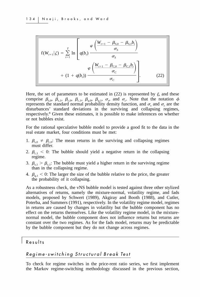
Exhibi t 4 � Maximum Likelihood Estimates from the Markov Regime-switching Model
Parameters Values Std. Err. p-values
2� 0 0.0001 0.0000 0.00002� 1 0.0011 0.0000 0.0002
�0 0.0027 0.0005 0.0000
�1 �0.0081 0.0049 0.1026
Log Likelihood 660.58
Notes: This table presents the parameter estimates, their standard errors, and the associatedp-values from the Markov-switching model:
P P� � a (1 � s ) � a s � (� (1 � s ) � � s )� ,� � � � 0 t 1 t 0 t 1 t tR Rt t�1
where P/R is the price-rent ratio, st is the state at time t, and �t is an error term.
estimating the parameters of equation (4) by maximum likelihood, and these arepresented in Exhibit 4. The results show that there are two distinct states: State 0represents a regime with relatively low volatility ( ) and a positive mean (�0).2�0
State 1, on the other hand, represents a regime that has a negative mean (�1) andhigher volatility ( ) in the price-rent ratio series. All the variables except for �1
2�1
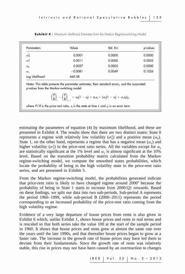
are statistically significant at the 1% level and �1 is almost significant at the 10%level. Based on the transition probability matrix calculated from the Markovregime-switching model, we compute the smoothed states probabilities, whichlocate the probability of being in the high volatility state in the price-rent ratioseries, and are presented in Exhibit 5.
From the Markov regime-switching model, the probabilities generated indicatethat price-rent ratio is likely to have changed regime around 20009 because theprobability of being in State 1 starts to increase from 2000:Q1 onwards. Basedon these findings, we split our data into two sub-periods. Sub-period A representsthe period 1960–1999, while sub-period B (2000–2011) represents the periodcorresponding to an increased probability of the price-rent ratio coming from thehigh volatility regime.
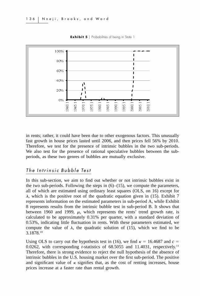
Evidence of a very large departure of house prices from rents is also given inExhibit 6 which, unlike Exhibit 1, shows house prices and rents in real terms andis rescaled so that both series take the value 100 at the start of the sample periodin 1960. It shows that house prices and rents grew at almost the same rate overthe years until the late 1990s, and that thereafter house prices began to grow at afaster rate. The increase in the growth rate of house prices may have led them todeviate from their fundamentals. Since the growth rate of rents was relativelystable, this rise in prices may not have been caused by an overreaction to changes
1 3 6 � N n e j i , B r o o k s , a n d W a r d
Exhibi t 5 � Probabilities of being in State 1
in rents; rather, it could have been due to other exogenous factors. This unusuallyfast growth in house prices lasted until 2006, and then prices fell 56% by 2010.Therefore, we test for the presence of intrinsic bubbles in the two sub-periods.We also test for the presence of rational speculative bubbles between the sub-periods, as these two genres of bubbles are mutually exclusive.
T h e I n t r i n s i c B u b b l e Te s t
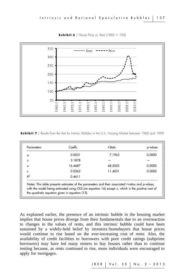
In this sub-section, we aim to find out whether or not intrinsic bubbles exist inthe two sub-periods. Following the steps in (6)–(15), we compute the parameters,all of which are estimated using ordinary least squares (OLS, on 16) except for�, which is the positive root of the quadratic equation given in (15). Exhibit 7represents information on the estimated parameters in sub-period A, while Exhibit8 represents results from the intrinsic bubble test in sub-period B. It shows thatbetween 1960 and 1999, �, which represents the rents’ trend growth rate, iscalculated to be approximately 0.31% per quarter, with a standard deviation of0.53%, indicating little fluctuation in rents. With these parameters estimated, wecompute the value of �, the quadratic solution of (15), which we find to be3.1878.10
Using OLS to carry out the hypothesis test in (16), we find � � 16.4687 and c �0.0262, with corresponding t-statistics of 68.5055 and 11.4031, respectively.11
Therefore, there is strong evidence to reject the null hypothesis of the absence ofintrinsic bubbles in the U.S. housing market over the first sub-period. The positiveand significant value of � signifies that, as the cost of renting increases, houseprices increase at a faster rate than rental growth.
I n t r i n s i c a n d R a t i o n a l S p e c u l a t i v e B u b b l e s � 1 3 7
J R E R � V o l . 3 5 � N o . 2 – 2 0 1 3
Exhibi t 6 � House Price vs. Rent (1960 � 100)
Exhibi t 7 � Results from the Test for Intrinsic Bubbles in the U.S. Housing Market between 1960 and 1999
Parameters Coeffs. t-Stats p-values
� 0.0031 7.1963 0.0000
� 3.1878 — —
� 16.4687 68.5055 0.0000
c 0.0262 11.4031 0.0000
R2 0.4611
Notes: This table presents estimates of the parameters and their associated t-ratios and p-values,with the model being estimated using OLS (on equation 16) except �, which is the positive root ofthe quadratic equation given in equation (15).
As explained earlier, the presence of an intrinsic bubble in the housing marketimplies that house prices diverge from their fundamentals due to an overreactionto changes in the values of rents, and this intrinsic bubble could have beensustained by a widely-held belief by investors/homebuyers that house priceswould continue to rise based on the ever-increasing cost of rents. Also, theavailability of credit facilities to borrowers with poor credit ratings (subprimeborrowers) may have led many renters to buy houses rather than to continuerenting because, as rents continued to rise, more individuals were encouraged toapply for mortgages.
1 3 8 � N n e j i , B r o o k s , a n d W a r d
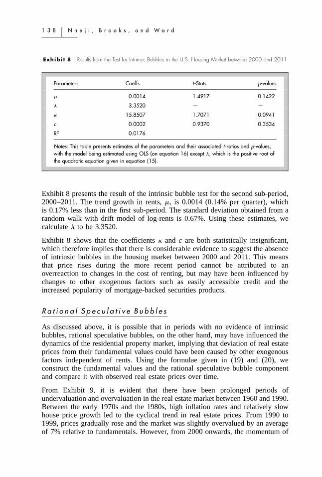
Exhibi t 8 � Results from the Test for Intrinsic Bubbles in the U.S. Housing Market between 2000 and 2011
Parameters Coeffs. t-Stats p-values
� 0.0014 1.4917 0.1422
� 3.3520 — —
� 15.8507 1.7071 0.0941
c 0.0002 0.9370 0.3534
R2 0.0176
Notes: This table presents estimates of the parameters and their associated t-ratios and p-values,with the model being estimated using OLS (on equation 16) except �, which is the positive root ofthe quadratic equation given in equation (15).
Exhibit 8 presents the result of the intrinsic bubble test for the second sub-period,2000–2011. The trend growth in rents, �, is 0.0014 (0.14% per quarter), whichis 0.17% less than in the first sub-period. The standard deviation obtained from arandom walk with drift model of log-rents is 0.67%. Using these estimates, wecalculate � to be 3.3520.
Exhibit 8 shows that the coefficients � and c are both statistically insignificant,which therefore implies that there is considerable evidence to suggest the absenceof intrinsic bubbles in the housing market between 2000 and 2011. This meansthat price rises during the more recent period cannot be attributed to anoverreaction to changes in the cost of renting, but may have been influenced bychanges to other exogenous factors such as easily accessible credit and theincreased popularity of mortgage-backed securities products.
R a t i o n a l S p e c u l a t i v e B u b b l e s
As discussed above, it is possible that in periods with no evidence of intrinsicbubbles, rational speculative bubbles, on the other hand, may have influenced thedynamics of the residential property market, implying that deviation of real estateprices from their fundamental values could have been caused by other exogenousfactors independent of rents. Using the formulae given in (19) and (20), weconstruct the fundamental values and the rational speculative bubble componentand compare it with observed real estate prices over time.
From Exhibit 9, it is evident that there have been prolonged periods ofundervaluation and overvaluation in the real estate market between 1960 and 1990.Between the early 1970s and the 1980s, high inflation rates and relatively slowhouse price growth led to the cyclical trend in real estate prices. From 1990 to1999, prices gradually rose and the market was slightly overvalued by an averageof 7% relative to fundamentals. However, from 2000 onwards, the momentum of
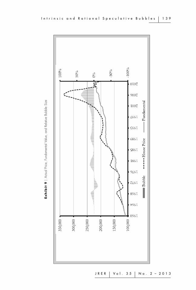
I n t r i n s i c a n d R a t i o n a l S p e c u l a t i v e B u b b l e s � 1 3 9
J R E R � V o l . 3 5 � N o . 2 – 2 0 1 3
Ex
hib
it9
�A
ctua
lPric
e,Fu
ndam
enta
lVal
ue,
and
Rela
tive
Bubb
leSi
ze
1 4 0 � N n e j i , B r o o k s , a n d W a r d
house price growth and the size of the rational speculative bubble componentrelative to prices increased significantly. This was due to the aggressive cuts ininterest rates following the collapse of the ‘‘dot-com’’ bubble in 2000. Accordingto Bankrate.com, the national average interest rate on 30-year fixed homemortgages fell by over 300 basis points between 2000 and 2005. In those fiveyears, the Mortgage Bankers Association noted that the number of mortgageapplications almost doubled, increasing the demand for homes. Similar to previousbubble episodes, individuals began to ‘‘flip’’ properties, as they believed that priceswould continue to rise.12 The number of mortgages given to borrowers who wereunable to qualify for conventional mortgages (nonprime or subprime borrowers)increased, and so at its peak in 2005 the real estate market was overvalued by38%.
However, from 2005, the Federal Reserve System began increasing interest ratesto reduce the inflationary pressure on the economy. The volume of residential realestate transactions fell as mortgage rates rose, thus slowing down the growth inprices. By 2009, foreclosures as a percentage of the total number of loans hadmore than tripled. Since then, the market has been undervalued.
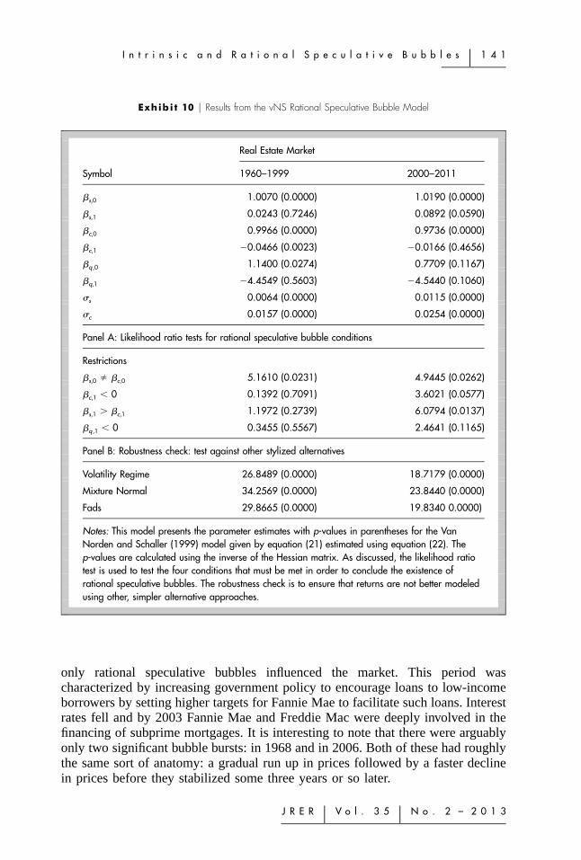
To determine whether the deviation of prices from fundamental values was dueto the presence of rational periodically collapsing speculative bubbles in the realestate market in either of the two sub-periods, we apply the vNS regime-switchingbubble model presented above. Exhibit 10 provides results from the vNS bubblemodel. The parameter estimates for the 1960–1999 period met only the first ofthe four rational speculative conditions listed in above (see the second panel ofExhibit 10), and thus there is strong evidence to conclude that rational speculativebubbles did not influence the market during this period. The 2000–2011 period,on the other hand, had clear signs of the existence of rational speculative bubblesas three of the four restrictions are met and the fourth is almost met at the 10%significance level.
Focusing on the sub-period 2000–2011, the average quarterly growth rate of realestate prices in the surviving regime (s,0) is 1.90% compared to negative 2.64%(i.e., 1 – 0.9736) in the collapsing regime. There is statistical evidence to showthat mean returns differ significantly across the two regimes. Also, the bubble inthe surviving regime yields greater returns than in the collapsing regime, as canbe seen by the signs of the coefficients of s,1 and c,1. Lastly, the significantnegative estimate of q,1 implies there is evidence that an increase in the size ofthe rational speculative bubble component relative to price increases theprobability of a collapse occurring. It is also important to note that the volatilityof returns in the market is greater in the collapsing regime (�c � 0.0254).Furthermore, rejections of the other stylized alternatives provide stronger evidenceto suggest that a rational speculative bubble influenced the real estate marketbetween 2000 and 2011 and that this model fits the data better than these simplerapproaches.
Therefore, there is significant information to conclude that intrinsic bubblesexisted in the real estate market between 1960 and 1999. Post-2000, however,
I n t r i n s i c a n d R a t i o n a l S p e c u l a t i v e B u b b l e s � 1 4 1
J R E R � V o l . 3 5 � N o . 2 – 2 0 1 3
Exhibi t 10 � Results from the vNS Rational Speculative Bubble Model
Real Estate Market
Symbol 1960–1999 2000–2011
s,0 1.0070 (0.0000) 1.0190 (0.0000)
s,1 0.0243 (0.7246) 0.0892 (0.0590)
c,0 0.9966 (0.0000) 0.9736 (0.0000)
c,1 �0.0466 (0.0023) �0.0166 (0.4656)
q ,0 1.1400 (0.0274) 0.7709 (0.1167)
q,1 �4.4549 (0.5603) �4.5440 (0.1060)
�s 0.0064 (0.0000) 0.0115 (0.0000)
�c 0.0157 (0.0000) 0.0254 (0.0000)
Panel A: Likelihood ratio tests for rational speculative bubble conditions
Restrictions
s,0 � c,0 5.1610 (0.0231) 4.9445 (0.0262)
c,1 � 0 0.1392 (0.7091) 3.6021 (0.0577)
s,1 � c,1 1.1972 (0.2739) 6.0794 (0.0137)
q ,1 � 0 0.3455 (0.5567) 2.4641 (0.1165)
Panel B: Robustness check: test against other stylized alternatives
Volatility Regime 26.8489 (0.0000) 18.7179 (0.0000)
Mixture Normal 34.2569 (0.0000) 23.8440 (0.0000)
Fads 29.8665 (0.0000) 19.8340 0.0000)
Notes: This model presents the parameter estimates with p-values in parentheses for the VanNorden and Schaller (1999) model given by equation (21) estimated using equation (22). Thep-values are calculated using the inverse of the Hessian matrix. As discussed, the likelihood ratiotest is used to test the four conditions that must be met in order to conclude the existence ofrational speculative bubbles. The robustness check is to ensure that returns are not better modeledusing other, simpler alternative approaches.
only rational speculative bubbles influenced the market. This period wascharacterized by increasing government policy to encourage loans to low-incomeborrowers by setting higher targets for Fannie Mae to facilitate such loans. Interestrates fell and by 2003 Fannie Mae and Freddie Mac were deeply involved in thefinancing of subprime mortgages. It is interesting to note that there were arguablyonly two significant bubble bursts: in 1968 and in 2006. Both of these had roughlythe same sort of anatomy: a gradual run up in prices followed by a faster declinein prices before they stabilized some three years or so later.
1 4 2 � N n e j i , B r o o k s , a n d W a r d
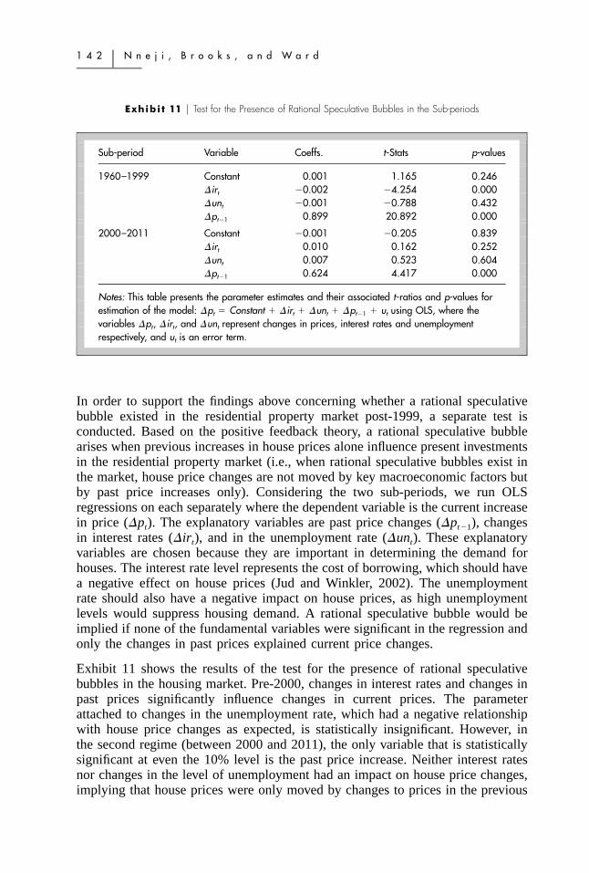
Exhibi t 11 � Test for the Presence of Rational Speculative Bubbles in the Sub-periods
Sub-period Variable Coeffs. t-Stats p-values
1960–1999 Constant 0.001 1.165 0.246�irt �0.002 �4.254 0.000�unt �0.001 �0.788 0.432�pt�1 0.899 20.892 0.000
2000–2011 Constant �0.001 �0.205 0.839�irt 0.010 0.162 0.252�unt 0.007 0.523 0.604�pt�1 0.624 4.417 0.000
Notes: This table presents the parameter estimates and their associated t-ratios and p-values forestimation of the model: �pt � Constant � �irt � �unt � �pt�1 � ut using OLS, where thevariables �pt, �irt, and �unt represent changes in prices, interest rates and unemploymentrespectively, and ut is an error term.
In order to support the findings above concerning whether a rational speculativebubble existed in the residential property market post-1999, a separate test isconducted. Based on the positive feedback theory, a rational speculative bubblearises when previous increases in house prices alone influence present investmentsin the residential property market (i.e., when rational speculative bubbles exist inthe market, house price changes are not moved by key macroeconomic factors butby past price increases only). Considering the two sub-periods, we run OLSregressions on each separately where the dependent variable is the current increasein price (�pt). The explanatory variables are past price changes (�pt�1), changesin interest rates (�irt), and in the unemployment rate (�unt). These explanatoryvariables are chosen because they are important in determining the demand forhouses. The interest rate level represents the cost of borrowing, which should havea negative effect on house prices (Jud and Winkler, 2002). The unemploymentrate should also have a negative impact on house prices, as high unemploymentlevels would suppress housing demand. A rational speculative bubble would beimplied if none of the fundamental variables were significant in the regression andonly the changes in past prices explained current price changes.
Exhibit 11 shows the results of the test for the presence of rational speculativebubbles in the housing market. Pre-2000, changes in interest rates and changes inpast prices significantly influence changes in current prices. The parameterattached to changes in the unemployment rate, which had a negative relationshipwith house price changes as expected, is statistically insignificant. However, inthe second regime (between 2000 and 2011), the only variable that is statisticallysignificant at even the 10% level is the past price increase. Neither interest ratesnor changes in the level of unemployment had an impact on house price changes,implying that house prices were only moved by changes to prices in the previous
I n t r i n s i c a n d R a t i o n a l S p e c u l a t i v e B u b b l e s � 1 4 3
J R E R � V o l . 3 5 � N o . 2 – 2 0 1 3
period and they no longer even have the correct signs. A Wald test is implementedto check for the joint significance of interest rates and unemployment in both sub-periods. We find a very low probability value in sub-period A, indicating thatunemployment levels and interest rates jointly influence changes in prices;however, in sub-period B, we find no evidence of joint significance.13 Hence, thereis evidence that a rational speculative bubble existed in the housing market duringthat period, as only appreciations in lagged prices significantly explain pricegrowth. House prices, based on the average price-rent ratio methodology forcomputing the fundamental value of houses, were overvalued by as much as 46%in 2006. The subsequent collapse of the rational speculative bubble saw houseprices fall by 37% between 2006 and 2009.
� D o R e n t s P r e d i c t C h a n g e s i n R e a l E s t a t e P r i c e s ?
Following the tests aimed at distinguishing between the types of bubble, weproceed to investigate the predictive nature of returns in the housing market. Asoutlined above, our aim is to establish whether or not changes in rents predictprice growth in times where intrinsic or rational bubbles exist. To perform thisanalysis, we first test for unit roots in the variables using the augmented Dickey-Fuller (ADF) test. If the variables have unit roots, then it could be the case thatthey are cointegrated. Cointegration implies that a linear combination of the twoseries would be integrated of order zero, or I(0), if the two variables are non-stationary. If both variables are non-stationary but not cointegrated, we wouldimplement a vector autoregressive (VAR) model on the first differences. Otherwisewe would use the vector error correction model (VECM). This is consistent withGranger’s (1986) conclusion that when variables are cointegrated, a VAR modelin differences would be mis-specified, whereas the VECM has the ability tocapture the deviations from the long-term equilibrium. Then a Granger causalitytest is employed to determine whether or not changes in rents predict the returnson investing in the U.S. housing market.
In order to test whether rents can predict returns in the housing market, the dataare again split into the same two sub-periods as above: ‘A’ representing the period1960–1999 and ‘B’ representing 2000–2011. Sub-period ‘A’ corresponds to thetime of an intrinsic bubble while ‘B’ is for the period where rational periodicallypartially collapsing speculative bubbles existed in the residential property market.This step will allow us to shed additional light on whether the traditionalrelationship between house prices and rents broke down post-2000 when therational bubble was in existence.
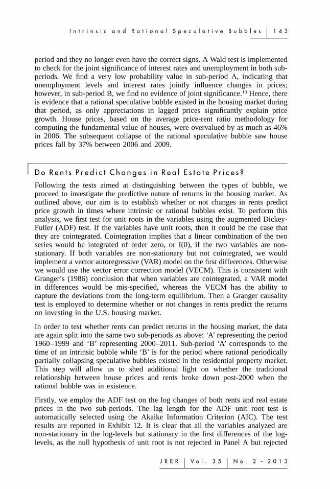
Firstly, we employ the ADF test on the log changes of both rents and real estateprices in the two sub-periods. The lag length for the ADF unit root test isautomatically selected using the Akaike Information Criterion (AIC). The testresults are reported in Exhibit 12. It is clear that all the variables analyzed arenon-stationary in the log-levels but stationary in the first differences of the log-levels, as the null hypothesis of unit root is not rejected in Panel A but rejected
1 4 4 � N n e j i , B r o o k s , a n d W a r d
Exhibi t 12 � Augmented Dickey-Fuller Unit Root Test for the Sub-periods
Sub-period Variables t-Stat. 5% Critical Value p-values
Panel A: Tests on the log levels
A: 1960–1999 Price �0.7488 �2.8801 0.8300Rent �1.2968 �2.8797 0.6305
B: 2000–2011 Price �2.4848 2.9458 0.1247Rent �2.0500 2.9297 0.2653
Panel B: Tests on the changes in the log-levels
A: 1960–1999 Price �4.7631 �3.4391 0.0008Rent �6.8679 �3.4385 0.0000
B: 2000–2011 Price �1.8952 �1.9496 0.0562Rent �4.8031 �1.9487 0.0000
Notes: This table presents the unit root test statistics along with the appropriate critical values atthe 5% significance level and the associated p-values. The null hypothesis that the variable has aunit root; Mackinnon, Haug, and Michelis (1999) p-values are employed.
Exhibi t 13 � Johansen’s Unrestricted Cointegration Rank (Trace) Test for the Sub-periods
Sub-period Null Trace Statistics 5% Critical Value p-values
A: 1960–1999 d � 0 20.8478 15.4947 0.0071d 1 2.2033 3.8415 0.1377
B: 2000–2011 d � 0 10.2812 15.4947 0.2597d 1 0.6487 3.8415 0.4206
Notes: The table presents the Johansen cointegration trace test statistics, the appropriate 5% criticalvalues and the associated p-values; d is the number of cointegrating vectors under the nullhypothesis; Mackinnon, Haug, and Michelis (1999) p-values are employed.
in Panel B. In Exhibit 13 we test for cointegration between the price and rentseries in their log-levels forms using the Johansen approach.
There is significant evidence to suggest that real estate prices and rents are foundto be cointegrated in sub-period A as the null hypotheses are rejected, indicatingthat there is at most one co-integrating equation. The Trace test on sub-period B,on the other hand, indicates no cointegration at the 5% level. Hence, we use aVECM model to analyze the first sub-period and a VAR for sub-period B.
I n t r i n s i c a n d R a t i o n a l S p e c u l a t i v e B u b b l e s � 1 4 5
J R E R � V o l . 3 5 � N o . 2 – 2 0 1 3
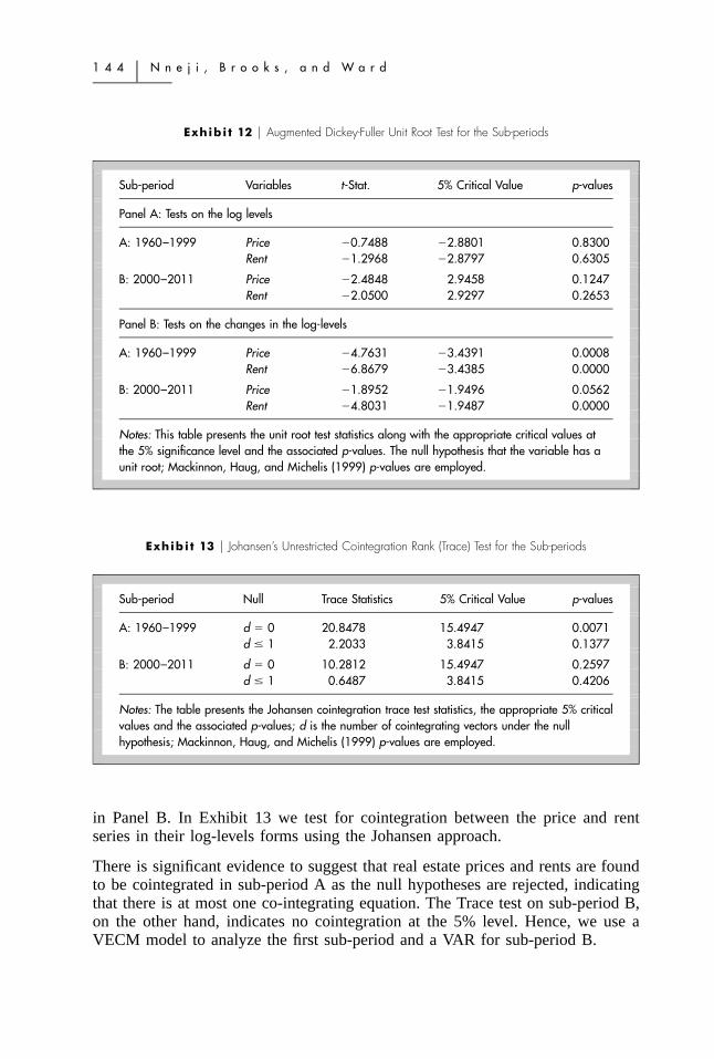
Exhibi t 14 � Granger Causality Test for the Sub-periods with Changes in House Prices as the
Dependent Variable
Sub-period Chi-Sq. p-values
A: 1960–1999 13.4649 0.0092
B: 2000–2011 0.0018 0.9660
Notes: This table presents the chi-squared critical values and associated p-values for Grangercausality tests constructed using a VAR model. The optimal lag lengths for the two models aredetermined by the AIC, and are found to be four and one in sub-periods A and B, respectively.
Using the coefficients obtained from the VAR and VECM models estimated, weaim to determine whether log changes in rents can predict real estate price growthby applying a Granger causality test. Note that the optimal lag length for the twomodels is determined by the AIC. We find that the optimum lag lengths for theVAR models in sub-periods A and B are four and one, respectively. Exhibit 14the results from the Granger causality tests on the two sub-periods.
It is very clear that changes in rents Granger-cause changes in real estate pricesonly during the period where there was an intrinsic bubble in the housing market.However, post-1999, there appears to be no causal relationship between changesin rents and the returns to investing in the residential housing market. This showsthat changes in rents can predict future real estate price changes only when thereis an intrinsic bubble; when only rational speculative bubbles exist, changes inrents do not predict returns. These findings confirm that house prices are moresensitive to changes in rents during periods when an intrinsic bubble is present.
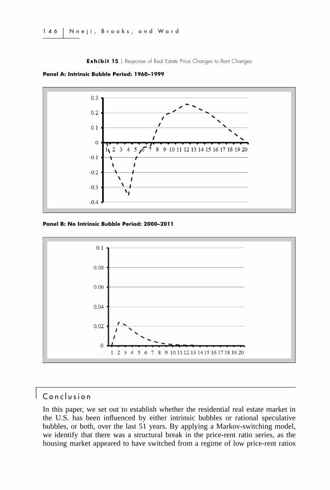
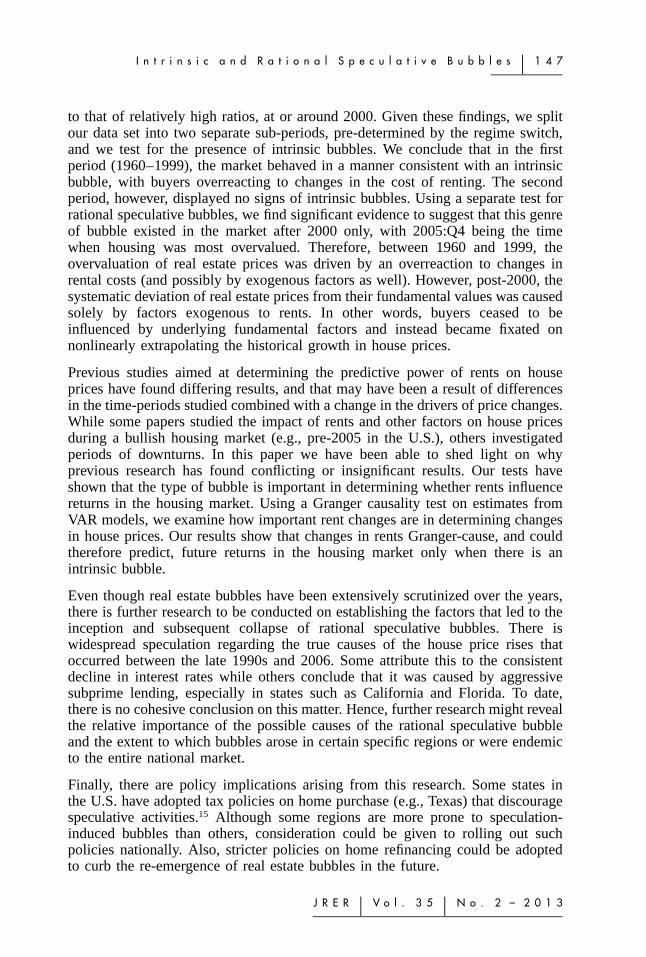
To further investigate the relationship between house prices and rents, we examinethe impulse response function of real estate prices to a positive unit shock in rentsin the two sub-periods for 20 quarters ahead. Exhibit 15 focuses on the degree ofsensitivity of real estate prices to changes in rents in the two sub-periods. Thegraphs provide further evidence supporting the intrinsic bubble model for theearlier sub-period. In the 1960–1999 period, unexpected increases in rental costcause prices to fall for the first seven quarters. From the eighth quarter onwards,the effect of rent innovation on real estate prices becomes positive. The effecteventually fizzles out around the twentieth quarter. For the 2000–2011 period, theeffect of unexpected changes in rental cost is far smaller14 than for the intrinsicbubble period, as prices do not react to any economically meaningful extentto changes in rents. It also takes a much shorter period (around nine quarters)for the effect of innovations to rental cost on real estate prices to die down tozero.
1 4 6 � N n e j i , B r o o k s , a n d W a r d
Exhibi t 15 � Response of Real Estate Price Changes to Rent Changes
Panel A: Intrinsic Bubble Period: 1960–1999
Panel B: No Intrinsic Bubble Period: 2000–2011
� C o n c l u s i o n
In this paper, we set out to establish whether the residential real estate market inthe U.S. has been influenced by either intrinsic bubbles or rational speculativebubbles, or both, over the last 51 years. By applying a Markov-switching model,we identify that there was a structural break in the price-rent ratio series, as thehousing market appeared to have switched from a regime of low price-rent ratios
I n t r i n s i c a n d R a t i o n a l S p e c u l a t i v e B u b b l e s � 1 4 7
J R E R � V o l . 3 5 � N o . 2 – 2 0 1 3
to that of relatively high ratios, at or around 2000. Given these findings, we splitour data set into two separate sub-periods, pre-determined by the regime switch,and we test for the presence of intrinsic bubbles. We conclude that in the firstperiod (1960–1999), the market behaved in a manner consistent with an intrinsicbubble, with buyers overreacting to changes in the cost of renting. The secondperiod, however, displayed no signs of intrinsic bubbles. Using a separate test forrational speculative bubbles, we find significant evidence to suggest that this genreof bubble existed in the market after 2000 only, with 2005:Q4 being the timewhen housing was most overvalued. Therefore, between 1960 and 1999, theovervaluation of real estate prices was driven by an overreaction to changes inrental costs (and possibly by exogenous factors as well). However, post-2000, thesystematic deviation of real estate prices from their fundamental values was causedsolely by factors exogenous to rents. In other words, buyers ceased to beinfluenced by underlying fundamental factors and instead became fixated onnonlinearly extrapolating the historical growth in house prices.
Previous studies aimed at determining the predictive power of rents on houseprices have found differing results, and that may have been a result of differencesin the time-periods studied combined with a change in the drivers of price changes.While some papers studied the impact of rents and other factors on house pricesduring a bullish housing market (e.g., pre-2005 in the U.S.), others investigatedperiods of downturns. In this paper we have been able to shed light on whyprevious research has found conflicting or insignificant results. Our tests haveshown that the type of bubble is important in determining whether rents influencereturns in the housing market. Using a Granger causality test on estimates fromVAR models, we examine how important rent changes are in determining changesin house prices. Our results show that changes in rents Granger-cause, and couldtherefore predict, future returns in the housing market only when there is anintrinsic bubble.
Even though real estate bubbles have been extensively scrutinized over the years,there is further research to be conducted on establishing the factors that led to theinception and subsequent collapse of rational speculative bubbles. There iswidespread speculation regarding the true causes of the house price rises thatoccurred between the late 1990s and 2006. Some attribute this to the consistentdecline in interest rates while others conclude that it was caused by aggressivesubprime lending, especially in states such as California and Florida. To date,there is no cohesive conclusion on this matter. Hence, further research might revealthe relative importance of the possible causes of the rational speculative bubbleand the extent to which bubbles arose in certain specific regions or were endemicto the entire national market.
Finally, there are policy implications arising from this research. Some states inthe U.S. have adopted tax policies on home purchase (e.g., Texas) that discouragespeculative activities.15 Although some regions are more prone to speculation-induced bubbles than others, consideration could be given to rolling out suchpolicies nationally. Also, stricter policies on home refinancing could be adoptedto curb the re-emergence of real estate bubbles in the future.
1 4 8 � N n e j i , B r o o k s , a n d W a r d
� E n d n o t e s1 More information on the construction of the data can be found at Land and Property
Values in the U.S., Lincoln Institute of Land Policy, http: / /www.lincolninst.edu/resources/ . While their approach to constructing the data is very sensible, it is possiblethat the interpolation and extrapolation methodology could cause some biases.
2 It is an interesting question as to whether or not intrinsic and periodically, partiallycollapsing rational bubbles can co-exist at the same time. Given that intrinsic bubblesare based on a nonlinear function of fundamental prices, and yet periodic, partiallycollapsing rational bubbles are based on the difference between actual prices andfundamentals, it seems as if they should be mutually exclusive, which is what we findempirically in the paper.
3 Although Markov-switching regression models date back to Goldfeld and Quandt(1973), we use the Hamilton (1994) approach, whereby the transition from one state toanother is modeled using a Markov chain. See Hamilton (1989, 1994) for more detailson how the probabilities are generated.
4 Of course, other nonlinear functional forms could be used here, and it is possible thata different functional form could lead to different results. However, we believe that theexponential form that is universally used in the current intrinsic bubble literature is notonly the most intuitive, it is also fairly flexible and covers a wide range of possibleshapes when both c and � are allowed to vary.
5 This implies that if � satisfies equation (14), then (8) clearly satisfies the definition ofthe bubble in (7). Therefore, this can be defined as an intrinsic bubble. Froot andObstfeld (1991) prove this mathematically in equation (13) on p. 1192 of their paper.
6 There would be collinearity amongst the explanatory variables if we decided to test forthe presence of an intrinsic bubble using P(Rt) � �Rt � cR .�
t
7 The derivation of equation (16) is fairly straightforward. Blanchard and Watson (1982)show that the expected size of the bubble in the next period is given as: E (B ) �t t�1
This is then re-arranged to give the stochastic processE (B �S)q � E (B �C)(1 � q).t t�1 t t�1
in (16).8 Note that in this study, the estimation of vNS’s bubble model is conducted using Matlab
7.9 and we use the Broyden (1970) (BFGS) method for solving optimization problemsthat are nonlinear.
9 This is in line with Lai and van Order’s (2010) finding that there was a regime shift inhouse prices, which saw a rise in momentum from 1999 onwards. In addition, it appearsas if there could be another regime switch around 1970 but unfortunately, this is tooclose to the start of the overall sample period and so splitting the data here would leavean insufficient number of observations before that date to estimate the models.
10 We must find � to be greater than one to show that a nonlinear explosive relationshipexists between the rents and bubbles. This would mean that house prices may overreactto changes in rents.
11 Prior to performing the intrinsic bubble test, we rescale the price and rent data, dividingeach data point by 1,000 so that the parameter estimates will be easier to interpret. Thiswill, of course, not change any of the significance levels or conclusions from theanalysis.

I n t r i n s i c a n d R a t i o n a l S p e c u l a t i v e B u b b l e s � 1 4 9
J R E R � V o l . 3 5 � N o . 2 – 2 0 1 3
12 The term ‘‘flip’’ is defined as purchasing and selling an asset within a short period oftime. An online article provided proof of this phenomenon occurring in the U.S. housingmarket: http: / /online.barrons.com/article/SB111905372884363176.html.
13 For sub-period A, the value of computed F-statistic is 3.371 with a correspondingprobability value of 0.047. Hence there is evidence to reject the null hypothesis of thejoint insignificance of interest rates and unemployment in predicting changes in houseprices. In sub-period B, however, the F-statistic is 1.973 with a probability value of0.139 and so we cannot reject the null hypothesis.
14 Note that the scale is approximately ten times smaller for Exhibit 15(b) than Exhibit15(a).
15 Miller, Sklarz, and Ordway (1988) examine a very intense, localized speculative episodethat occurred in Hawaii during the late 1980s.
� R e f e r e n c e s
Abraham, J. and P. Hendershott. Bubbles in Metropolitan Housing Markets. Journal ofHousing Research, 1996, 7, 191–207.
Akgiray, V. and G.G. Booth. Mixed Diffusion-jump Process Modelling of Exchange RateMovements. Review of Economics and Statistics, 1988, 70, 631–37.
Baddeley, M. Housing Bubbles, Herds and Frenzies: Evidence from British HousingMarkets, CCEPP Policy Brief, 02–05. Cambridge Centre for Economic and Public Policy,Cambridge, 2005.
Black, A., P. Fraser, and M. Hoesli. House Prices, Fundamentals and Bubbles. Journal ofBusiness Finance and Accounting, 2006, 33, 1535–55.
Bjorklund, K. and B. Soderberg. Property Cycle, Speculative Bubbles and the Gross IncomeMultiplier. Journal of Real Estate Research, 1999, 18, 151–74.
Blanchard, O. and M. Watson, Bubbles, rational expectations, and financial markets. In:Wachtel, P. (ed.), Crisis in the Economic and Financial Structure. Lexington Books,Lexington, MA, 1982.
Broyden, C.G. The Convergence of a Class of Double-rank Minimization Algorithms 1.General Considerations. Journal of Applied Math, 1970, 6, 197076-90.
Brooks, C. and A. Katsaris. A Three-regime Model of Speculative Behaviour: Modellingthe Evolution of Bubbles in the S&P 500 Composite Index. Economic Journal, 2005a,115, 767–97.
——. Trading Rules from Forecasting the Collapse of Speculative Bubbles for the S&P500 Composite Index. Journal of Business, 2005b, 78, 2003–36.
Brooks, C., A. Katsaris, T. McGough, and S. Tsolacos. Testing for Bubbles in IndirectProperty Price Cycles. Journal of Property Research, 2001, 18, 341–56.
Campbell, S.D., M.A. Davis, J. Gallin, and R.F. Martin. What Moves Housing Markets: AVariance Decomposition of the Rent-Price Ratio. Journal of Urban Economics, 2009, 66,90–102.
Case, K.E. and R.J. Shiller. Is There a Bubble in the Housing Market? Brookings Paperson Economic Activity, 2004, 2, 299–342.
Cutler, D.M., J.M. Poterba, and L.H. Summers, Speculative dynamics, Review of EconomicStudies, 1991, 58, 529–546.
1 5 0 � N n e j i , B r o o k s , a n d W a r d
Davis, M.A., A. Lehnert, and F.M. Robert. The Rent-Price Ratio for the Aggregate Stockof Owner-occupied Housing. Review of Income and Wealth, 2008, 54, 279–84.
Diba, B.T. and H.I. Grossman. Explosive Rational Bubbles in Stock Prices? AmericanEconomic Review, 1988, 78, 520–30.
Englund, P., M. Hwang, and J.M. Quigley. Hedging Housing Risk. Journal of Real EstateFinance and Economics, 2002, 24, 167–200.
Fraser, P., M. Hoesli, and L. McAlevey. A Comparative Analysis of House Prices andBubbles in the U.K. and New Zealand. Pacific Rim Property Research Journal, 2008, 14,257–78.
Froot, K.A. and M. Obstfeld. Intrinsic Bubbles: The Case of Stock Prices. AmericanEconomic Review, 1991, 81, 1189–1224.
Gallin, J. The Long-run Relationship between House Prices and Rents. Finance andEconomics Discussion Series, 2004–50. Board of Governors of the Federal ReserveSystem, Washington, DC, September 2004.
Garber, P.M. Famous First Bubbles. Journal of Economic Perspectives, 1990, 4, 35–54.
Gilberto, S.M. A Note on Commercial Mortgage Flows and Construction. Journal of RealEstate Research, 1992, 7, 485–92.
Goldfeld, S.M. and R.E. Quandt. A Markov Model for Switching Regressions. Journal ofEconometrics, 1973, 1, 3–15.
Goodman, A.C. and T.G. Thibodeau. Where are the Speculative Bubbles in the U.S.Housing Markets? Journal of Housing Economics, 2008, 17, 117–37.
Granger, C.W.J. Developments in the Study of Cointegrated Economic Variables. OxfordBulletin of Economics and Statistics, 1986, 42, 213–27.
Hamilton, J.D. A New Approach of the Economic Analysis of Nonstationary Time Seriesand the Business Cycle. Econometrica, 1989, 57, 357–84.
Hamilton, J.D. Time Series Analysis. Princeton University Press, Princeton, NJ, 1994.
Hatzvi, E. and G. Otto. Prices, Rents and Rational Speculative Bubbles in the SydneyHousing Market. Economic Record, 2008, 84, 405–20.
Helbling, T. and M. Terrones. When Bubbles Burst. In World Economy Outlook. ChapterII, International Monetary Fund, Washington, DC, 2003, 61–94.
Hendershott, P. Property Asset Bubbles: Evidence from the Sydney Office Market. Journalof Real Estate Finance and Economics, 2000, 20, 67–81.
Jirasakuldech, B., R. Campbell, and L. Knight. Are There Rational Speculative Bubbles inREITs? Journal of Real Estate Finance and Economics, 2006, 32, 105–07.
Jud, G.D. and D.R. Winkler. The Dynamics of Metropolitan Housing Prices. Journal ofReal Estate Research, 2002, 23, 29–45.
Kim, K.-H. and H.S. Lee. Real Estate Price Bubble and Price Forecasts in Korea.Department of Economics, Sogang University, 2000.
Lai, R.N. and R.A. van Order. Momentum and House Price Growth in the United States:Anatomy of a Bubble. Real Estate Economics, 2010, 38, 753–73.
Ma, Y. and A. Kanas. Intrinsic Bubbles Revisited: Evidence from Nonlinear Cointegrationand Forecasting. Journal of Forecasting, 2004, 23, 237–50.
MacKinnon, J.G., M.A. Haug, and L. Michelis. Numerical Distribution Functions ofLikelihood Ratio Tests for Cointegration, Journal of Applied Econometrics, 1999, 14, 563–577.
I n t r i n s i c a n d R a t i o n a l S p e c u l a t i v e B u b b l e s � 1 5 1
J R E R � V o l . 3 5 � N o . 2 – 2 0 1 3
Mankiw, N.G. and D.N. Weil. The Baby Boom, the Baby Bust, and the Housing Market.Regional Science and Urban Economics, 1989, 19, 235–58.
Mikhed, V. and P. Zemcik. Testing for Bubbles in Housing Markets: A Panel DataApproach. Journal of Real Estate Finance and Economics, 2009, 38, 366–86.
Miller, N.G., M.A. Sklarz, and N. Ordway. Japanese Purchases, Exchange Rates, andSpeculation in Residential Real Estate Markets. Journal of Real Estate Research, 1988, 3,39–49.
Pavlidis, E., I. Paya, D. Peel, and A. Spiru. Bubbles in House Prices and Their Impact onConsumption: Evidence for the U.S. Technical report, Lancaster University ManagementSchool, 2009.
Payne, J. and G. Waters. REIT Markets: Periodically Collapsing Negative Bubbles? AppliedFinancial Economic Letters, 2005, 1, 65–9.
Payne, J. and G. Waters. Have Equity REITs Experienced Periodically Collapsing Bubbles?Journal of Real Estate Finance and Economics, 2007, 34, 207–24.
Rapach, D.E. and J.K. Strauss. The Long-run Relationship between Consumption andHousing Wealth in the Eighth District States. Regional Economic Development, 2006, 2,140–47.
Roche, M.J. The Rise in House Prices in Dublin: Bubble, Fad or Just Fundamentals.Economic Modelling, 2001, 18, 281–95.
Schwert, G.W. Business Cycles, Financial Crises and Stock Volatility. Carnegie-RochesterConference Series on Public Policy, 1989, 31, 83–126.
Van Norden, S. and H. Schaller. The Predictability of Stock Market Regime: Evidencefrom the Toronto Stock Exchange. Review of Economics and Statistics, 1993, 75, 505–10.
Van Norden, S. and H. Schaller. Speculative Behaviour, Regime-Switching, and StockMarket Crashes. In P. Rothman (ed.), Nonlinear Time Series Analysis of Economic andFinancial Data. Norwell, MA: Kluwer Academic Publishers, 1999, 321–56.
Wheaton, W.C. and G. Nechayev. The 1998–2005 Housing ‘‘Bubble’’ and the Current‘‘Correction’’: What’s Different This Time? Journal of Real Estate Research, 2008, 30, 1–26.
Zhou, W.X. and D. Sornette. Is There a Real Estate Bubble in the U.S.? Physica A, 2006,361, 297–308.
The authors would like to thank four anonymous reviewers for their helpfulsuggestions. We would also like to thank Apostolos Katsaris for providing the Matlabcode to estimate the van Norden and Schaller model.
Ogonna Nneji, University of Reading, Whiteknights, Reading UK RG6 6BA [email protected].
Chris Brooks, University of Reading, Whiteknights, Reading UK RG6 6BA [email protected].
Charles Ward, University of Reading, Whiteknights, Reading UK RG6 6BA [email protected].
