intro to deep learning - autoencoders

COE-416Seminar

Autoencoders for Unsupervised Learning in

Deep Neural Networks

By:

Akash Goel2K12/CO/009

Deep Learning is based on

Neural Networks

History of Neural Networks1943- Neurophysiologist Warren McCulloch and mathematician Walter Pitts wrote a paper on how neurons might work.

1949- Donald Hebb, famous Canadian psychologist, wrote “The Organization of Behavior”, a work which pointed out the fact that neural pathways are strengthened each time they are used (Hebbian Learning)

1959 - Bernard Widrow and Marcian Hoff of Stanford developed models called "ADALINE" and "MADALINE." - developed to recognize binary patterns and eliminate echoes on phone lines

1975 - Kohonen and Anderson developed the first multilayered network

1986 - Rumelhart, D. E., Hinton, G. E., and Williams, R. J. authored a seminal paper, which showed how backpropagation algorithm can be used to train neural networks with multiple layers quickly.

Artificial Neural Networks(Multilayer Perceptron)

• Artificial neural networks are generally presented as systems of interconnected "neurons" which exchange messages between each other.

• The connections have numeric weights that can be tuned based on experience, making neural nets adaptive to inputs and capable of learning.

• An artificial neuron is a mathematical function conceived as a model of biological neurons. They constitute an artificial neural network.

• The artificial neuron receives one or more inputs (representing dendrites) and produces an output (representing a neuron's axon).

• Usually the sums of each node are weighted, and the sum is passed through a non-linear function known as an activation function or transfer function.

• The transfer functions usually have a sigmoid shape, but they may also take the form of other non-linear functions, piecewise linear functions, or step functions.

Artificial Neuron

Architecture Neuron Model

An elementary neuron with R inputs is shown below. Each input is weighted with an appropriate w. The sum of the weighted inputs and the bias forms the input to the transfer function f. Neurons can use any differentiable transfer function f to generate their output.

Architecture Neuron Model

Transfer Function (Activation Function)

Multilayer networks often use non-linear activation functions like the sigmoid transfer function.

The sigmoid function generates outputs between 0 and 1 as the neuron's net input goes from negative to positive infinity.

An example of a Neural Network

Architecture - Feedforward NetworkFeedforward networks often have one or more hidden layers of sigmoid neurons followed by an output layer of linear neurons.

Multiple layers of neurons with nonlinear transfer functions allow the network to learn nonlinear and linear relationships between input and output vectors.

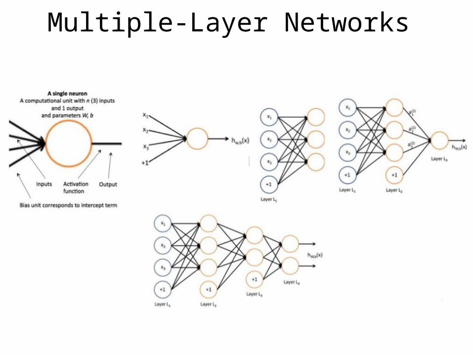
Multiple-Layer Networks

Learning

Input vectors (x) and the corresponding target vectors (y) are used to train a network until it can approximate a function, called cost function, and thus associate input vectors with specific output vectors, or classify input vectors in an appropriate way as defined by us.

For this purpose, the backpropagation algorithm (Hinton, et al, 1986) is generally empoyed.

Learning - Schematic

Backpropagation • To teach the neural network we need training data set. The training data set

consists of input signals(x ) assigned with corresponding target (desired output) y.

• The network training is an iterative process. In each iteration weight coefficients of nodes are modified using new data from training data set.

• Each teaching step starts with selecting examples from the training set. After this stage we can determine output signals values for each neuron in each network layer. The errors are calculated at the output later and propagated back to the first layer. These errors give the gradient of the cost function, which is used to alter the weights at each layer according to the formula:

Gradient Descent - Intuition

Backpropagation employs Local Gradient Descent for its optimization technique.

Learning Algorithm:Backpropagation

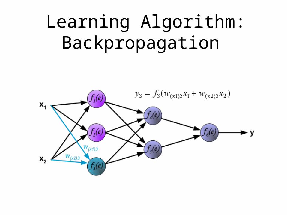
The following slides describes teaching process of multi-layer neural network employing backpropagation algorithm. To illustrate this process the three layer neural network with two inputs and one output,which is shown in the picture below, is used:


Pictures below illustrate how signal is propagating through the network, Symbols w(xm)n represent weights of connections between network input xm and neuron n in input layer. Symbols yn represents output signal of neuron n.


Propagation of signals through the hidden layer. Symbols wmn represent weights of connections between output of neuron m and input of neuron n in the next layer.


Propagation of signals through the output layer.


In the next algorithm step the output signal of the network y is compared with the desired output value (the target), which is found in training data set. The difference is called error signal d of output layer neuron


The idea is to propagate error signal d (computed in single teaching step) back to all neurons, which output signals were input for discussed neuron.


The weights' coefficients wmn used to propagate errors back are equal to this used during computing output value. Only the direction of data flow is changed (signals are propagated from output to inputs one after the other). This technique is used for all network layers. If propagated errors came from few neurons they are added. The illustration is below:


When the error signal for each neuron is computed, the weights coefficients of each neuron input node may be modified. In formulas below df(e)/de represents derivative of neuron activation function (which weights are modified).

Advantages of Multilayer Perceptrons:

1. Adaptive learning: An ability to learn how to do tasks based on the data given for training or initial experience.

2. One of the preferred techniques for gesture recognition.

3. MLP/Neural networks do not make any assumption regarding the underlying probability density functions or other probabilistic information about the pattern classes under consideration in comparison to other probability based models.

4. They yield the required decision function directly via training.

5. A two layer backpropagation network with sufficient hidden nodes has been proven to be a universal approximator (i.e., they can represent a wide variety of interesting functions when given appropriate parameters).

Shortcomings • Too shallow to learn complex relationships and structures in data

• Can be surpassed by other “traditional” learning approaches (e.g. SVMs) at the cost less complex models.

• Cannot train deep networks

• Requires supervised learning, which is based on carefully crafted datasets. This is not a trivial task.

Deep Learning

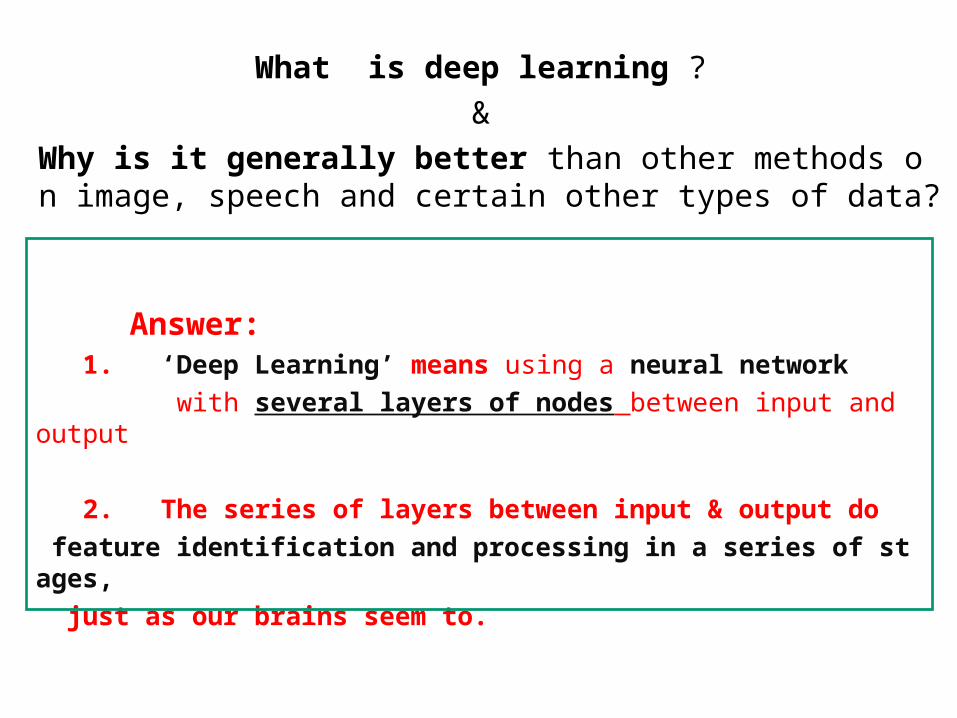
What is deep learning ? &

Why is it generally better than other methods on image, speech and certain other types of data?

Answer: 1. ‘Deep Learning’ means using a neural network with several layers of nodes between input and output 2. The series of layers between input & output do feature identification and processing in a series of stages, just as our brains seem to.

How is it different from Multilayer neural networks ?

We have had good algorithms for learning theweights in networks with 1 hidden layer

But these algorithms are not good at learning the weights fornetworks with more hidden layers

which requires new algorithms for training many-later networks

Motivations for Deep Learning• Deep Architectures can be representationally efficient– Fewer computational units for same function

• Deep Representations might allow for a hierarchy orrepresentation– Allows non-local generalization– Comprehensibility

• Multiple levels of latent variables allow combinatorialsharing of statistical strength

• Deep architectures work well (vision, audio, NLP, etc.)

Deep learning: A brief history In 1979, Kunihiko Fukushima invented an artificial neural network, "Neocognitron", which has a hierarchical multilayered architecture and acquires the ability to recognize visual patterns through learning.

In 1989, Yann LeCun et al. were able to apply the standard backpropagation algorithm, which had been around since 1974, to a deep neural network with the purpose of recognizing handwritten ZIP codes on mail.

Despite the success of applying the algorithm, the time to train the network on this dataset was approximately 3 days, making it impractical for general use.

In 2006, after a publication by Geoffrey Hinton and Ruslan Salakhutdinov showed how a many-layered feedforward neural network could be effectively pre-trained one layer at a time.

In late 2009, Li Deng invited Geoffrey Hinton to work with him and colleagues at Microsoft Research to apply deep learning to speech recognition.They co-organized the 2009 NIPS Workshop on Deep Learning for Speech Recognition.

It was discovered that given large amounts of data, deep learning techniques can out-perform all other techniques for such tasks. Thus, deep-learning evolved to become the accepted standard for advanced machine learning today.

Problems with Back Propagation

• It requires labeled training data.–Almost all data is unlabeled.

• The learning time does not scale well–It is very slow in networks with multiple hidden layers.

• It can get stuck in poor local optima.–These are often quite good, but for deep nets they are far from optimal.

Deep Neural Networks• Simple to construct– Sigmoid nonlinearity for hidden layers– Softmax for the output layer

• But, backpropagation does not work well (if randomly initialized)– Deep networks trained with backpropagation (without unsupervised pretraining) perform worse than shallow networks (Bengio et al., NIPS 2007)

Autoencoders

(a step towards deep learning)

So far, we have described the application of neural networks to supervised learning, in which we are have labeled training examples. Now suppose we have only unlabeled training examples set :

{x (1) ,x (2) ,x (3) ,...}, where x (i) ∈Rn .

An autoencoder neural network is an unsupervised learning algorithm that applies backpropagation, setting the target values to be equal to the inputs. I.e., it uses y (i) = x (i) .

Example of an autoencoder

(Hidden)

The autoencoder tries to learn the identity function

h(x)=x

by placing constraints on the network, such as :

1. Limiting the number of hidden units, we can discover interesting (density constraint)2. Letting the number of hidden units be large (greater than the number of input pixels)(sparsity constaint)

This helps them to learn interesting structure in data.

Visualization• Having trained an autoencoder, we would now like to

visualize the function learned by the algorithm, to try to understand what it has learned.

• Consider the case of training an autoencoder on 10 × 10 images, so that n = 100. Each hidden unit i computes a function of the input:

Visualization (2)When we do this for a sparse autoencoder (trained with 100 hidden units on 10x10 pixel inputs) we get the following result:

(Each box is the image that maximally activates that neuron.)

Stacked (deep) Autoencoders• Stacking layers of autoencoders (or RBMs),

produces a deeper architecture known as Stacked or Deep Autoencoders.

• Applications: Face recognition, Speech recognition, Signal Denoising, etc.

Learning in Stacked Autoencoders

In general, autoencoders are stacked one over the other to learn complex features from the data.

The backpropagation algorithm is also applied for learning in autoencoders. The only difference is that learning is done by pretraining of each layer before its successor.

Denoising autoencoders: In order to force the hidden layer to discover more robust features and prevent it from simply learning the identity, we train the autoencoder to reconstruct the input from a corrupted version of it.

Denoising autoencoder

The image shows how a "denoising" autoencoder may be used to generate correct input from corrupted input.

corrupt input cleaned input

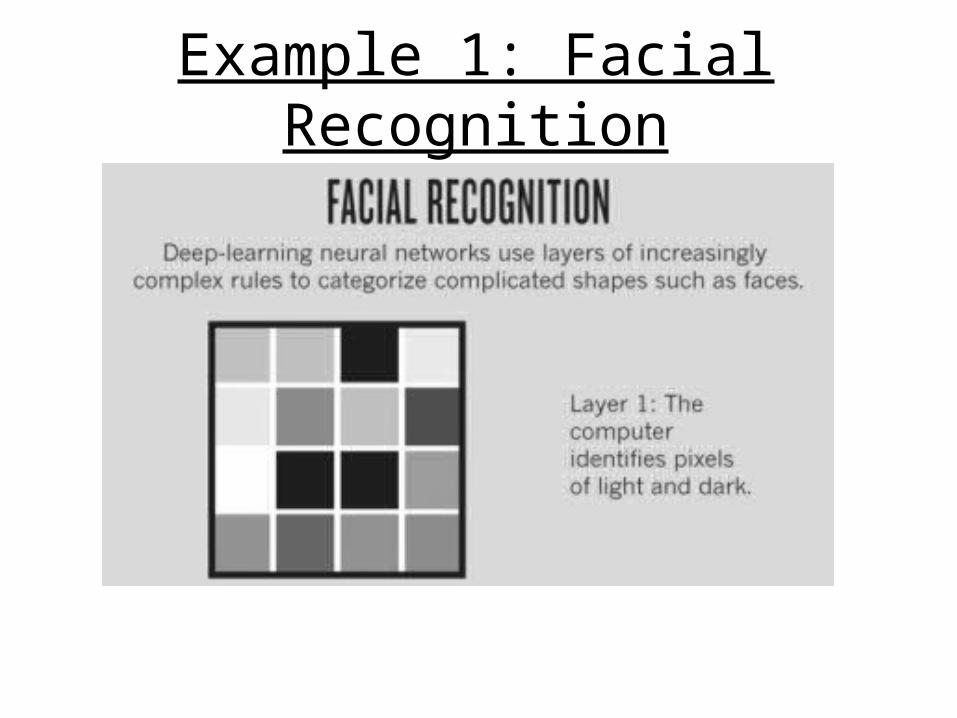
Example 1: Facial Recognition

Example 2: Document retrieval(Information representation and classification)

• We can use an autoencoder to find low-dimensional codes for documents that allow fast and accurate retrieval of similar documents from a large set.

• We start by converting each document into a “bag of words”. This a 2000 dimensional vector that contains the counts for each of the 2000 commonest words.

How to compress the count vector

• We train the neural network to reproduce its input vector as its output

• This forces it to compress as much information as possible into the 10 numbers in the central bottleneck.

• These 10 numbers are then a good way to compare documents.–See Ruslan Salakhutdinov’s talk

2000 reconstructed counts

500 neurons

2000 word counts

500 neurons

250 neurons

250 neurons

10

input vector

output vector

Using autoencoders to visualize documents

• Instead of using codes to retrieve documents, we can use 2-D codes to visualize sets of documents.

2000 reconstructed counts

500 neurons

2000 word counts

500 neurons

250 neurons

250 neurons

2

input vector

output vector

Using PCA

(Principal Component Analysis)

First compress all documents to 2 numbers using a type of PCA

Then use different colors for different document categories

Using Autoencoders

First compress all documents to 2 numbers with an autoencoder. Then use different colors for different document categories

A really fast way to find similar documents

• Suppose we could convert each document into a binary feature vector in such a way that similar documents have similar feature vectors.–This creates a “semantic” address space that allows us to use the memory bus for retrieval.

• Given a query document we first use the autoencoder to compute its binary address. –Then we fetch all the documents from addresses that are within a small radius in hamming space.–This takes constant time. No comparisons are required for getting the shortlist of semantically similar documents.

Bibliography• 1986 Rumelhart, D. E., Hinton, G. E., and Williams, R. J.

“Learning representations by back-propagating errors.”• 2006 Hinton, G. E. and Salakhutdinov, R. R “Reducing

the dimensionality of data with neural networks.”• 2007 Hinton, G. E.

“Learning multiple layers of representation.”• 2011 Andrew Ng(CS294A )

“Sparse autoencoder”

Bibliography• 1991 Sepp Hochrieter

“Untersuchungen zu dynamischen neuronalen Netzen”

• 2009 Salakhutdinov, Ruslan.“Learning deep generative models”

• 2016 Michael Nielsen“Neural Networks and Deep Learning”

• 2016 Ian Goodfellow, Yoshua Bengio and Aaron Courville“Deep Learning”

intro to deep learning - autoencoders

Technology