Mathematisch-Naturwissenschaftliche Fakultät

Eldar Sultanow, Denis Volkov, Sean Cox

Introducing a Finite State Machine for processing Collatz Sequences

Universität Potsdam

Preprint published at the Institutional Repository of the Potsdam University:http://nbn-resolving.de/urn:nbn:de:kobv:517-opus4-399223

Contents

1 Introduction . . . . . . . . . . . . . . . . . . . . . . . . . . . . . . . . . . . . . . . . . . . . . . . . . . . . . . . . . 3

1.1 Motivation 3

1.2 Related Research 3

2 Dependent Threads State Machine . . . . . . . . . . . . . . . . . . . . . . . . . . . . . . . . . . . . 6

2.1 Introducing a Dependent Threads State Machine (DTSM) 6

2.2 The Collatz DTSM 6

2.3 Series of State Transition Sequences 8

3 Conclusion and Outlook . . . . . . . . . . . . . . . . . . . . . . . . . . . . . . . . . . . . . . . . . . . . . 14

3.1 Summary 14

3.2 Outlook 14

Literature . . . . . . . . . . . . . . . . . . . . . . . . . . . . . . . . . . . . . . . . . . . . . . . . . . . . . . . . . . 15

1

1. Introduction

The present work will introduce a Finite State Machine (FSM) that processes any Collatz Se-quence; further, we will endeavor to investigate its behavior in relationship to transformationsof a special infinite input. Moreover, we will prove that the machines word transformationis equivalent to the standard Collatz number transformation and subsequently discuss thepossibilities for use of this approach at solving similar problems. The benefit of this approachis that the investigation of the word transformation performed by the Finite State Machine isless complicated than the traditional number-theoretical transformation.

1.1 Motivation

The Collatz conjecture is a number theoretical problem, which has puzzled countless re-searchers using myriad approaches. Presently, there are scarcely any methodologies to de-scribe and treat the problem from the perspective of the Algebraic Theory of Automata. Suchan approach is promising with respect to facilitating the comprehension of the Collatz se-quences "mechanics". The systematic technique of a state machine is both simpler and canfully be described by the use of algebraic means.

The current gap in research forms the motivation behind the present contribution. Thepresent authors are convinced that exploring the Collatz conjecture in an algebraic manner,relying on findings and fundamentals of Automata Theory, will simplify the problem as awhole.

1.2 Related Research

The Collatz conjecture is one of the unsolved mathematical Millennium problems [1]. WhenLothar Collatz began his professorship in Hamburg in 1952, he mentioned this problem tohis colleague Helmut Hasse. From 1976 to 1980, Collatz wrote several letters but missedreferencing that he first proposed the problem in 1937. He introduced a function g :N→Nas follows:

g(x) =

3x +1 2 ∤ x

x/2 otherwise(1.1)

This function is surjective, but it is not injective (for example g(3) = g(20)) and thus it is notreversible.

In his book The Ultimate Challenge: The 3x+1 Problem [2], along with his annotatedbibliographies [3], [4] and othermanuscripts like an earlier paper from 1985, [5] Lagarias has

3

4 1.2. Related Research

reseached and put together different approaches from various authors intended to describeand solve the Collatz conjecture.

For the integers up to 2,367,363,789,863,971,985,761 the conjecture holds valid. Forinstance, see the computation history given by Kahermanes [6] that provides a timeline ofthe results which have already been achieved.

Inverting the Collatz sequence and constructing a Collatz tree is an approach that hasbeen carried out by many researchers. It is well known that inverse sequences [7] arisefrom all functions h ∈ H , which can be composed of the two mappings q, r : N → N withq :m 7→ 2m and r :m 7→ (m− 1)/3: H = {h :N→N | h = r(j) ◦ q(i) ◦ . . . , i, j,h(1) ∈N}

An argumentation that the Collatz Conjecture cannot be formally proved can be foundin the work of Craig Alan Feinstein [8], who presents the position that any proof of theCollatz conjecturemust have an infinite number of lines and thus no formal proof is possible.However, this statement will not be acknowledged in depth within this study.

Treating Collatz sequences in a binary system can be performed as well. For example,Ethan Akin [9] handles the Collatz sequence with natural numbers written in base 2 (us-ing the Ring Z2 of two-adic integers), because divisions by 2 are easier to deal with in thismethod. He uses a shift map σ on Z2 and a map τ:

σ(x) =

(x − 1)/2 2 ∤ x

x/2 otherwiseτ(x) =

(3x +1)/2 2 ∤ x

x/2 otherwise

The shift map’s fundamental property is σ(x)i = xi+1, noting that σ(x)i is the i-th digitof σ(x). This property can easily be comprehended by an example x = 5 = 1010000 . . . =x0x1x2 . . ., containing σ(x) = 2 = 0100000 . . .

Akin then defines a transformation Q : Z2→ Z2 by Q(x)i = τi(x)0 for non-negative inte-gers i which means Q(x)i is zero if τi(x) is even and then it is one in any other instance. Thistransformation is a bijective map that defines a conjugacy between τ and σ : Q ◦ τ = σ ◦Qand it is equivalent to the map denoted Q∞ by Lagarias [5] and it is the inverse of the mapΦ introduced by Bernstein [10]. Q can be described as follows: Let x be a 2-adic integer.The transformation result Q(x) is a 2-adic integer y, so that yn = τ(n)(x)0. This means, thefirst bit y0 is the parity of x = τ(0)(x), which is one, if x is odd and otherwise zero. The nextbit y1 is the parity of τ(1)(x), and the bit after next y2 is parity of τ ◦ τ(x) and so on. Theconjugancy Q ◦ τ = σ ◦Q can be demonstrated by transforming the expression as follows:(σ ◦Q(x))i =Q(x)i+1 = τ(i+1)(x)0 = τ(i)(τ(x))0 =Q(τ(x))i

A simulation of the Collatz function by Turing machines has been presented by Michel[11]. He introduces Turing machines that simulate the iteration of the Collatz function,where he considers them having 3 states and 4 symbols. Michel examines both turing ma-chines, those that never halt and those that halt on the final loop.

A function-theoretic approach this problem has been provided by Berg and Meinardus[12], [13] as well as Gerhard Opfer [14], who consistently relies on the Bergs and Meinardusidea. Opfer tries to prove the Collatz conjecture by determining the kernel intersection oftwo linear operators U, V that act on complex-valued functions. First he determined thekernel of V, and then he attempted to prove that its image by U is empty. Benne de Weger[15] contradicted Opfers attempted proof.

Reachability Considerations based on a Collatz tree exist as well. It is well known thatthe inverted Collatz sequence can be represented as a graph; to be more specific, they can be

Chapter 1. Introduction 5

depicted as a tree [16], [17]. It is acknowledged that in order to prove the Collatz conjecture,then one needs to demonstrate that this tree covers all (odd) natural numbers.

The Stopping Time theory has been introduced by Terras [18], [19], [20]. He introducesanother notation of the Collatz function T (n) = (3X(n)n +X(n))/2, where X(n) = 1 when n isodd and X(n) = 0 when n is even, and defined the stopping time of n, denoted by χ(n), as theleast positive k for which T (k)(n) < n, if it exists, or otherwise it reaches infinity. Let Li be aset of natural numbers, it is observable that the stopping time exhibits the regularity χ(n) = ifor all n fulfilling n ≡ l(mod2i ), l ∈ Li , L1 = {4}, L2 = {5}, L4 = {3}, L5 = {11,23}, L7 = {7,15,59}and so on. As i increases, the sets Li , including their elements, become significantly larger.Sets Li are empty when i ≡ l(mod19) for l = 3,6,9,11,14,17,19. Additionally, the largestelement of a non-empty set Li is always less than 2i .

Many other approaches exist as well. From an algebraic perspective Trümper [21] ana-lyzes The Collatz Problem in light of an Infinite Free Semigroup. Kohl [22] generalized theproblem by introducing residue class-wise affine, in short, by utilizing rcwa mappings. Apolynomial analogue of the Collatz Conjecture has been provided by Hicks et al. [23] [24]and there are also stochastical, statistical and Markov chain-based and permutation-basedapproaches to proving this elusive theory.

2. Dependent Threads State Machine

2.1 Introducing a Dependent Threads State Machine (DTSM)

Let us regard a Finite State Machine (Σ,S, s0,δ,F ∈ S), Σ as the input alphabet, S a set ofstates, s0 the starting state, F a set of final states, and δ : S ×Σ→ S the transition function.We may concisely write δ0(x) = δ(x,0) : S→ S .

Definition 2.1 A DTSM (Dependent Threads State Machine) is a finite state machinethat has the following properties:

1. Σ = {0,1}, the input alphabet consists of two elements called bits. It is a binaryalphabet.

2. F = {f0}, the DTSM has only one final state.

3. δ0(s0) = s0, the DTSM remains in its starting state when inputting zero.

4. ∀s ∈ S\{s0} : ∃n ≥ 0,δ(n)0 (s) = f0, if the DTSM is in any state except s0, a continuousinput of zero leads to guaranteed f0.

5. A transition S ×Σ→ S is considered synonymous with a directed edge. Any bitthat is an input of the function δ and thus a value of the corresponding edge,we call a δ-bit. Additionally, we label each edge with an ϵ-bit using a functionϵ : S ×Σ→ Σ. The meaning of this labeling will be explored later.

It may be noted that the term "State Machine" can be treated as synonymous to the term"Automaton" (plural Automata). Hence, a Finite State Machine (FSM) may also be denotedas Finite State Automaton (FSA). In accordance with the automata theory, a FSM belongs toa special set of the Turing machines respective to all Turing machines.

2.2 The Collatz DTSM

The Collatz DTSM is an example of a DTSM and defined by four states S = {s,a,b, c} and thefunctions δ, ϵ provided by table 2.1. The positions that are inputs of both functions δ and ϵare the source positions, not the target positions.

6

Chapter 2. Dependent Threads State Machine 7

δ 0 1s s ca a bb a cc b c

ϵ 0 1s 0 0a 0 1b 1 0c 0 1

Table 2.1: Definition of the both functions δ and ϵ

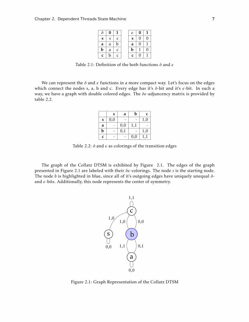
We can represent the δ and ϵ functions in a more compact way. Let’s focus on the edgeswhich connect the nodes s, a, b and c. Every edge has it’s δ-bit and it’s ϵ-bit. In such away, we have a graph with double colored edges. The δϵ-adjuncency matrix is provided bytable 2.2.

s a b cs 0,0 - - 1,0a - 0,0 1,1 -b - 0,1 - 1,0c - - 0,0 1,1

Table 2.2: δ and ϵ as colorings of the transition edges

The graph of the Collatz DTSM is exhibited by Figure 2.1. The edges of the graphpresented in Figure 2.1 are labeled with their δϵ-colorings. The node s is the starting node.The node b is highlighted in blue, since all of it’s outgoing edges have uniquely unequal δ-and ϵ-bits. Additionally, this node represents the center of symmetry.

s

0,0

c

1,1

1,0

b

0,01,0

a

0,0

0,11,1

Figure 2.1: Graph Representation of the Collatz DTSM

8 2.3. Series of State Transition Sequences

2.3 Series of State Transition Sequences

Allow us to regard a binary sequence (dk)k∈N0defined by a mapping D : N→ Σ that has a

finite preimage D−1(1). In other words, a natural k exists, for which all m ≥ k are mapped tozero D(m) = 0 and thus all sequence members dm are zero. This binary sequence describesthe DTSM’s state transitions starting from s. Hence the sequence members correspond tothe δ-bits. In accordance to the DTSM definition, this sequence must end up and remaineternally in the state a. The following example illustrates the state transitions of the DTSM.

Exempel 2.1 Assume we have a sequence (dk) = (1,0,1,0,1,0,1,1,0,1,0,0,0 . . .). Thissequence generates a sequence of DTSM positions (pk) = (c,b, c,b, c,b, c, c,b, c,b,a,a, . . . ).

It is important to point out that for an input bit dk the corresponding position pk is the target position intowhich the token moves to and not the source position from which the tokens moves from. Hence we considerthe starting position s to have a negative index −1, which in our notation means p−1 = s.

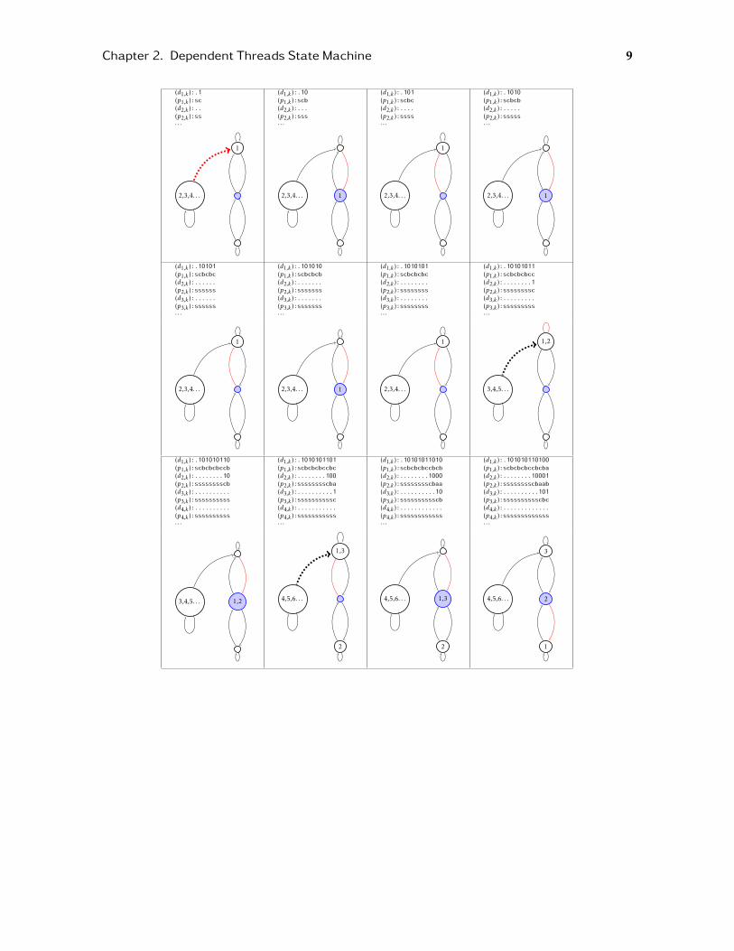
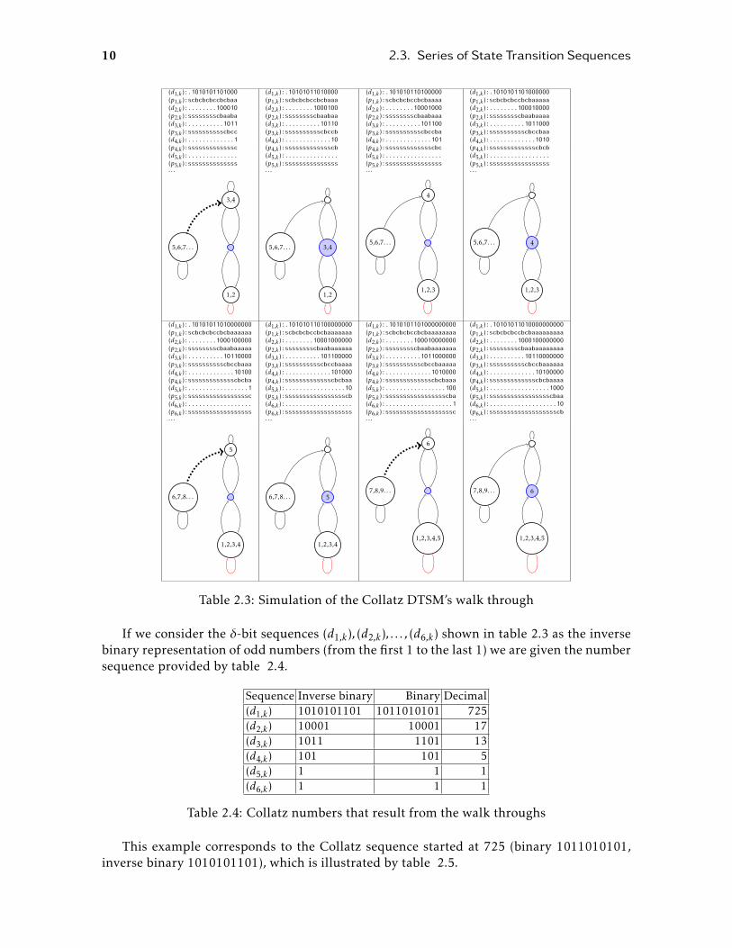
The ϵ-bit, an edge is labeled with, belongs to a sequence of ϵ-bits that result from theDTSM’s state transitions. A sequence of δ-bits describes a sequence of state transitionsthrough the DTSM’s edges beginning at the starting node s. The sequence of ϵ-bits is de-fined by the order of passed edges in the walk through, which each naturally are specifiedby (labeled with) an ϵ-bit. A sequence of ϵ-bits forms the sequence of δ-bits describing thestate transitions for the next walk through. This continuing principle is illustrated by ta-ble 2.3, which provides a simulative description (state by state) of these consecutive walkthroughs up to 10101011010000000000.

The latter binary sequence is the δ-bit sequence of the first walk through. All other δ-bitsequences arise from the ϵ-bits of those edges that are traversed during this and subsequentwalkthroughs. For example, the ϵ-bits of traversed edges by the second walk through formthe sequence of δ-bits for the third walk through and beyond.

Along the δ-bit sequences, table 2.3 portrays the corresponding sequences of DTSM po-sitions, which have been walked through up to their respective states.

In table 2.3 we can reproduce and verify the repeated application of ϵ-bit sequences. Ifwe take a closer look at the example (p1,k) which is the sequence of DTSM positions describ-ing the first token’s walk through, that generates the ϵ-bit sequence 00000001000100000000.This bit sequence corresponds to the δ-bit sequence (d2,k) that defines the walk through ofthe second token.

Red colored edges indicate the first token’s walk through. The edge between the startingnode s and the node c is highlighted dotted, when a new token becomes active by leavingthe starting node, respectively moving to c.

Chapter 2. Dependent Threads State Machine 9

(d1,k ):.1 (d1,k ):.10 (d1,k ):.101 (d1,k ):.1010(p1,k ):sc (p1,k ):scb (p1,k ):scbc (p1,k ):scbcb(d2,k ):.. (d2,k ):... (d2,k ):.... (d2,k ):.....(p2,k ):ss (p2,k ):sss (p2,k ):ssss (p2,k ):sssss· · · · · · · · · · · ·

2,3,4. . .

1

2,3,4. . . 1 2,3,4. . .

1

2,3,4. . . 1

(d1,k ):.10101 (d1,k ):.101010 (d1,k ):.1010101 (d1,k ):.10101011(p1,k ):scbcbc (p1,k ):scbcbcb (p1,k ):scbcbcbc (p1,k ):scbcbcbcc(d2,k ):...... (d2,k ):....... (d2,k ):........ (d2,k ):........1(p2,k ):ssssss (p2,k ):sssssss (p2,k ):ssssssss (p2,k ):ssssssssc(d3,k ):...... (d3,k ):....... (d3,k ):........ (d3,k ):.........(p3,k ):ssssss (p3,k ):sssssss (p3,k ):ssssssss (p3,k ):sssssssss· · · · · · · · · · · ·

2,3,4. . .

1

2,3,4. . . 1 2,3,4. . .

1

3,4,5. . .

1,2

(d1,k ):.101010110 (d1,k ):.1010101101 (d1,k ):.10101011010 (d1,k ):.101010110100(p1,k ):scbcbcbccb (p1,k ):scbcbcbccbc (p1,k ):scbcbcbccbcb (p1,k ):scbcbcbccbcba(d2,k ):........10 (d2,k ):........100 (d2,k ):........1000 (d2,k ):........10001(p2,k ):sssssssscb (p2,k ):sssssssscba (p2,k ):sssssssscbaa (p2,k ):sssssssscbaab(d3,k ):.......... (d3,k ):..........1 (d3,k ):..........10 (d3,k ):..........101(p3,k ):ssssssssss (p3,k ):ssssssssssc (p3,k ):sssssssssscb (p3,k ):sssssssssscbc(d4,k ):.......... (d4,k ):........... (d4,k ):............ (d4,k ):.............(p4,k ):ssssssssss (p4,k ):sssssssssss (p4,k ):ssssssssssss (p4,k ):sssssssssssss· · · · · · · · · · · ·

3,4,5. . . 1,2 4,5,6. . .

1,3

2

4,5,6. . . 1,3

2

4,5,6. . .

3

2

1

10 2.3. Series of State Transition Sequences

(d1,k ):.1010101101000 (d1,k ):.10101011010000 (d1,k ):.101010110100000 (d1,k ):.1010101101000000(p1,k ):scbcbcbccbcbaa (p1,k ):scbcbcbccbcbaaa (p1,k ):scbcbcbccbcbaaaa (p1,k ):scbcbcbccbcbaaaaa(d2,k ):........100010 (d2,k ):........1000100 (d2,k ):........10001000 (d2,k ):........100010000(p2,k ):sssssssscbaaba (p2,k ):sssssssscbaabaa (p2,k ):sssssssscbaabaaa (p2,k ):sssssssscbaabaaaa(d3,k ):..........1011 (d3,k ):..........10110 (d3,k ):..........101100 (d3,k ):..........1011000(p3,k ):sssssssssscbcc (p3,k ):sssssssssscbccb (p3,k ):sssssssssscbccba (p3,k ):sssssssssscbccbaa(d4,k ):.............1 (d4,k ):.............10 (d4,k ):.............101 (d4,k ):.............1010(p4,k ):sssssssssssssc (p4,k ):ssssssssssssscb (p4,k ):ssssssssssssscbc (p4,k ):ssssssssssssscbcb(d5,k ):.............. (d5,k ):............... (d5,k ):................ (d5,k ):.................(p5,k ):ssssssssssssss (p5,k ):sssssssssssssss (p5,k ):ssssssssssssssss (p5,k ):sssssssssssssssss· · · · · · · · · · · ·

5,6,7. . .

3,4

1,2

5,6,7. . . 3,4

1,2

5,6,7. . .

4

1,2,3

5,6,7. . . 4

1,2,3

(d1,k ):.10101011010000000 (d1,k ):.101010110100000000 (d1,k ):.1010101101000000000 (d1,k ):.10101011010000000000(p1,k ):scbcbcbccbcbaaaaaa (p1,k ):scbcbcbccbcbaaaaaaa (p1,k ):scbcbcbccbcbaaaaaaaa (p1,k ):scbcbcbccbcbaaaaaaaaa(d2,k ):........1000100000 (d2,k ):........10001000000 (d2,k ):........100010000000 (d2,k ):........1000100000000(p2,k ):sssssssscbaabaaaaa (p2,k ):sssssssscbaabaaaaaa (p2,k ):sssssssscbaabaaaaaaa (p2,k ):sssssssscbaabaaaaaaaa(d3,k ):..........10110000 (d3,k ):..........101100000 (d3,k ):..........1011000000 (d3,k ):..........10110000000(p3,k ):sssssssssscbccbaaa (p3,k ):sssssssssscbccbaaaa (p3,k ):sssssssssscbccbaaaaa (p3,k ):sssssssssscbccbaaaaaa(d4,k ):.............10100 (d4,k ):.............101000 (d4,k ):.............1010000 (d4,k ):.............10100000(p4,k ):ssssssssssssscbcba (p4,k ):ssssssssssssscbcbaa (p4,k ):ssssssssssssscbcbaaa (p4,k ):ssssssssssssscbcbaaaa(d5,k ):.................1 (d5,k ):.................10 (d5,k ):.................100 (d5,k ):.................1000(p5,k ):sssssssssssssssssc (p5,k ):ssssssssssssssssscb (p5,k ):ssssssssssssssssscba (p5,k ):ssssssssssssssssscbaa(d6,k ):.................. (d6,k ):................... (d6,k ):...................1 (d6,k ):...................10(p6,k ):ssssssssssssssssss (p6,k ):sssssssssssssssssss (p6,k ):sssssssssssssssssssc (p6,k ):ssssssssssssssssssscb· · · · · · · · · · · ·

6,7,8. . .

5

1,2,3,4

6,7,8. . . 5

1,2,3,4

7,8,9. . .

6

1,2,3,4,5

7,8,9. . . 6

1,2,3,4,5

Table 2.3: Simulation of the Collatz DTSM’s walk through

If we consider the δ-bit sequences (d1,k), (d2,k), . . . , (d6,k) shown in table 2.3 as the inversebinary representation of odd numbers (from the first 1 to the last 1) we are given the numbersequence provided by table 2.4.

Sequence Inverse binary Binary Decimal(d1,k) 1010101101 1011010101 725(d2,k) 10001 10001 17(d3,k) 1011 1101 13(d4,k) 101 101 5(d5,k) 1 1 1(d6,k) 1 1 1

Table 2.4: Collatz numbers that result from the walk throughs

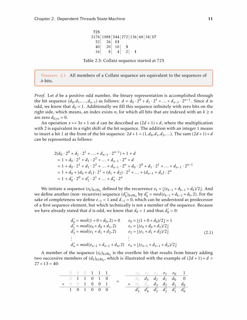
This example corresponds to the Collatz sequence started at 725 (binary 1011010101,inverse binary 1010101101), which is illustrated by table 2.5.

Chapter 2. Dependent Threads State Machine 11

7252176 1088 544 272 136 68 34 17

52 26 1340 20 10 516 8 4 2 1

Table 2.5: Collatz sequence started at 725

Theorem 2.1 All members of a Collatz sequence are equivalent to the sequences ofδ-bits.

Proof. Let d be a positive odd number, the binary representation is accomplished throughthe bit sequence (d0,d1, . . . ,dn−1) as follows: d = d0 · 20 + d1 · 21 + . . . + dn−1 · 2n−1. Since d isodd, we know that d0 = 1. Additionally we fill this sequence infinitely with zero bits on theright side, which means, an index exists n, for which all bits that are indexed with an k ≥ nare zero dk≥n = 0.

An operation x 7→ 3x + 1 on d can be described as (2d + 1) + d, where the multiplicationwith 2 is equivalent to a right shift of the bit sequence. The addition with an integer 1 meansto insert a bit 1 at the front of the bit sequence: 2d +1 = (1,d0,d1,d2, . . .). The sum (2d +1)+dcan be represented as follows:

2(d0 · 20 + d1 · 21 + . . . + dn−1 · 2n−1) + 1 + d

= 1 + d0 · 21 + d1 · 22 + . . . + dn−1 · 2n + d

= 1 + d0 · 21 + d1 · 22 + . . . + dn−1 · 2n + d0 · 20 + d1 · 21 + . . . + dn−1 · 2n−1

= 1 + d0 + (d0 + d1) · 21 + (d1 + d2) · 22 + . . . + (dn−1 + dn) · 2n

= 1 + d ′0 · 20 + d ′1 · 2

1 + . . . + d ′n · 2n

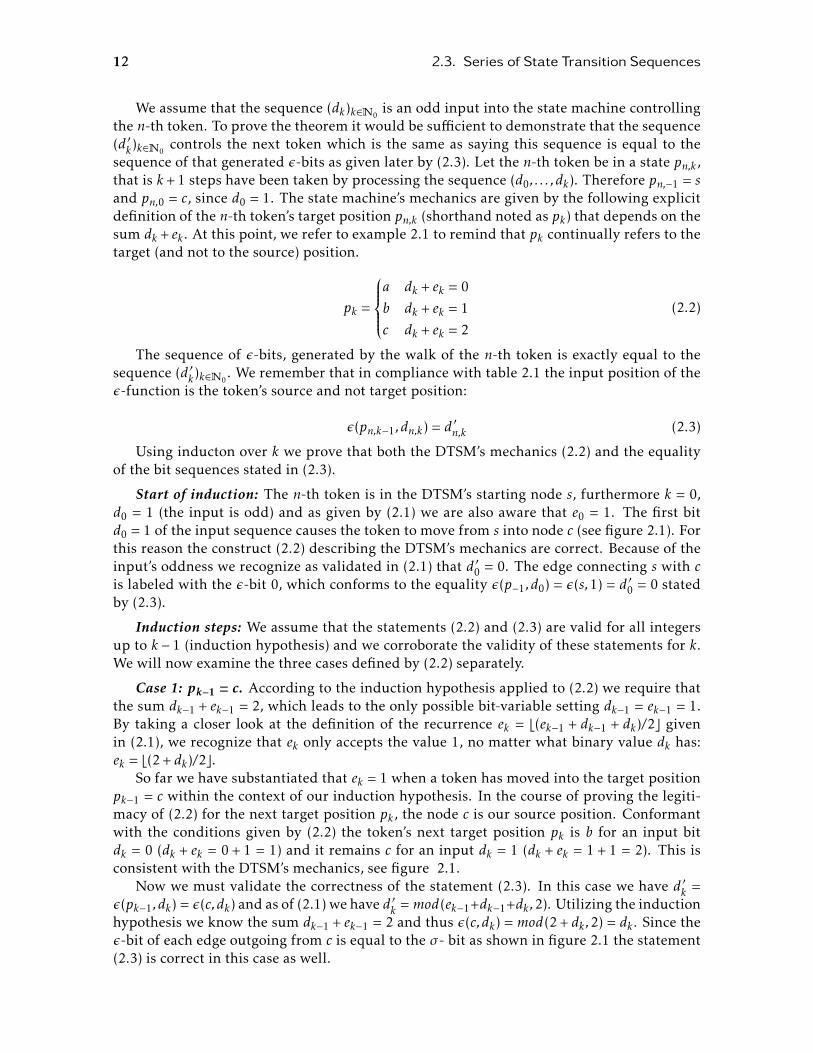
We initiate a sequence (ek)k∈N0defined by the recurrence ek = ⌊(ek−1 + dk−1 + dk)/2⌋. And

we define another (non- recursive) sequence (d ′k)k∈N0by d ′k =mod(ek−1 +dk−1 +dk ,2). For the

sake of completeness we define e−1 = 1 and d−1 = 0, which can be understood as predecessorof a first sequence element, but which technically is not a member of the sequence. Becausewe have already stated that d is odd, we know that d0 = 1 and thus d ′0 = 0:

d ′0 =mod(1 + 0+ d0,2) = 0 e0 = ⌊(1 + 0+ d0)/2⌋ = 1d ′1 =mod(e0 + d0 + d1,2) e1 = ⌊(e0 + d0 + d1)/2⌋d ′2 =mod(e1 + d1 + d2,2) e2 = ⌊(e1 + d1 + d2)/2⌋...

...d ′n =mod(en−1 + dn−1 + dn,2) en = ⌊(en−1 + dn−1 + dn)/2⌋

(2.1)

A member of the sequence (ek)k∈N0is the overflow bit that results from binary adding

two successive members of (dk)k∈N0, which is illustrated with the example of (2d + 1) + d =

27+13 = 40:

0 0 0 1 1 10 1 1 0 1 0

+ 0 0 1 0 0 11 0 1 0 0 0

=

e4 e3 e2 e1 e0 1d4 d3 d2 d1 d0 0

+ d5 d4 d3 d2 d1 d0d ′5 d ′4 d ′3 d ′2 d ′1 d ′0

12 2.3. Series of State Transition Sequences

We assume that the sequence (dk)k∈N0is an odd input into the state machine controlling

the n-th token. To prove the theorem it would be sufficient to demonstrate that the sequence(d ′k)k∈N0

controls the next token which is the same as saying this sequence is equal to thesequence of that generated ϵ-bits as given later by (2.3). Let the n-th token be in a state pn,k ,that is k +1 steps have been taken by processing the sequence (d0, . . . ,dk). Therefore pn,−1 = sand pn,0 = c, since d0 = 1. The state machine’s mechanics are given by the following explicitdefinition of the n-th token’s target position pn,k (shorthand noted as pk) that depends on thesum dk + ek . At this point, we refer to example 2.1 to remind that pk continually refers to thetarget (and not to the source) position.

pk =

a dk + ek = 0

b dk + ek = 1

c dk + ek = 2

(2.2)

The sequence of ϵ-bits, generated by the walk of the n-th token is exactly equal to thesequence (d ′k)k∈N0

. We remember that in compliance with table 2.1 the input position of theϵ-function is the token’s source and not target position:

ϵ(pn,k−1,dn,k) = d ′n,k (2.3)

Using inducton over k we prove that both the DTSM’s mechanics (2.2) and the equalityof the bit sequences stated in (2.3).

Start of induction: The n-th token is in the DTSM’s starting node s, furthermore k = 0,d0 = 1 (the input is odd) and as given by (2.1) we are also aware that e0 = 1. The first bitd0 = 1 of the input sequence causes the token to move from s into node c (see figure 2.1). Forthis reason the construct (2.2) describing the DTSM’s mechanics are correct. Because of theinput’s oddness we recognize as validated in (2.1) that d ′0 = 0. The edge connecting s with cis labeled with the ϵ-bit 0, which conforms to the equality ϵ(p−1,d0) = ϵ(s,1) = d ′0 = 0 statedby (2.3).

Induction steps: We assume that the statements (2.2) and (2.3) are valid for all integersup to k − 1 (induction hypothesis) and we corroborate the validity of these statements for k.We will now examine the three cases defined by (2.2) separately.

Case 1: pk−1 = c. According to the induction hypothesis applied to (2.2) we require thatthe sum dk−1 + ek−1 = 2, which leads to the only possible bit-variable setting dk−1 = ek−1 = 1.By taking a closer look at the definition of the recurrence ek = ⌊(ek−1 + dk−1 + dk)/2⌋ givenin (2.1), we recognize that ek only accepts the value 1, no matter what binary value dk has:ek = ⌊(2 + dk)/2⌋.

So far we have substantiated that ek = 1 when a token has moved into the target positionpk−1 = c within the context of our induction hypothesis. In the course of proving the legiti-macy of (2.2) for the next target position pk , the node c is our source position. Conformantwith the conditions given by (2.2) the token’s next target position pk is b for an input bitdk = 0 (dk + ek = 0 + 1 = 1) and it remains c for an input dk = 1 (dk + ek = 1 + 1 = 2). This isconsistent with the DTSM’s mechanics, see figure 2.1.

Now we must validate the correctness of the statement (2.3). In this case we have d ′k =ϵ(pk−1,dk) = ϵ(c,dk) and as of (2.1) we have d ′k =mod(ek−1+dk−1+dk ,2). Utilizing the inductionhypothesis we know the sum dk−1 + ek−1 = 2 and thus ϵ(c,dk) =mod(2 + dk ,2) = dk . Since theϵ-bit of each edge outgoing from c is equal to the σ- bit as shown in figure 2.1 the statement(2.3) is correct in this case as well.

Chapter 2. Dependent Threads State Machine 13

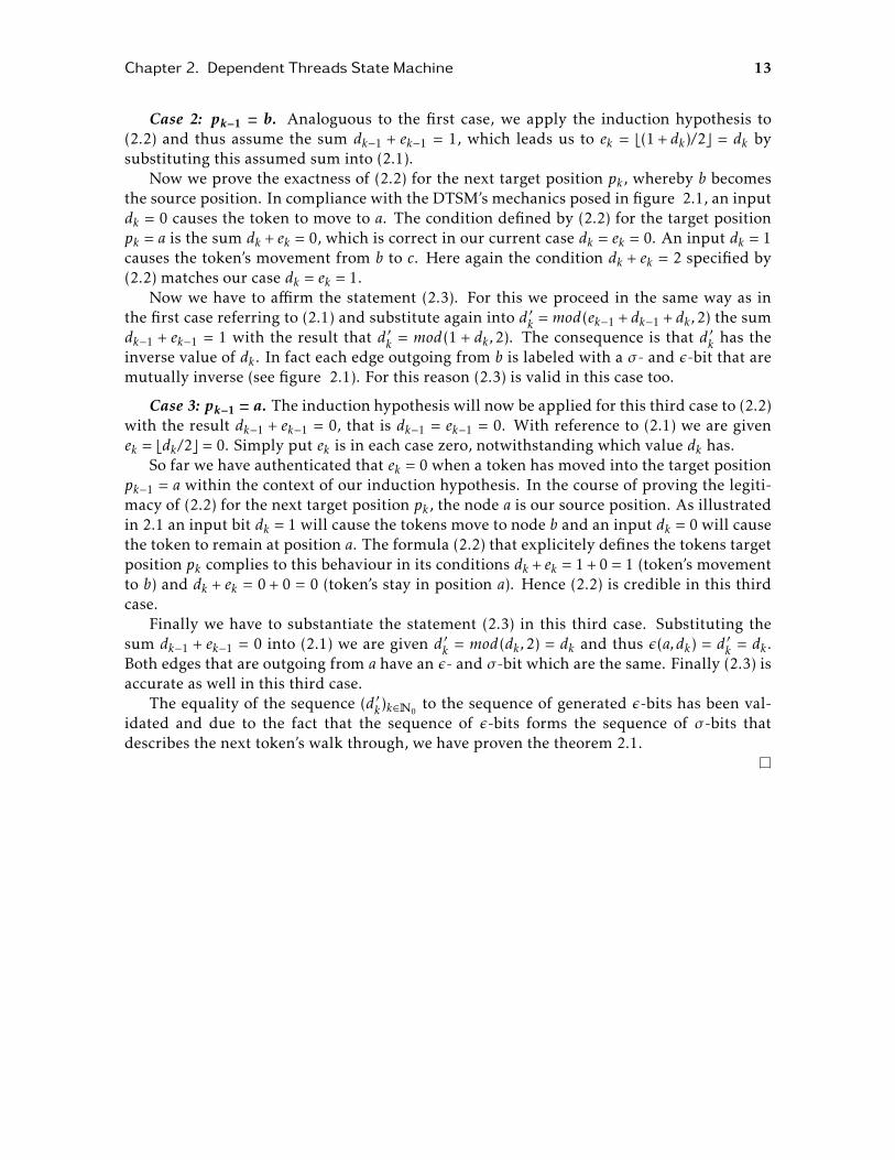
Case 2: pk−1 = b. Analoguous to the first case, we apply the induction hypothesis to(2.2) and thus assume the sum dk−1 + ek−1 = 1, which leads us to ek = ⌊(1 + dk)/2⌋ = dk bysubstituting this assumed sum into (2.1).

Now we prove the exactness of (2.2) for the next target position pk , whereby b becomesthe source position. In compliance with the DTSM’s mechanics posed in figure 2.1, an inputdk = 0 causes the token to move to a. The condition defined by (2.2) for the target positionpk = a is the sum dk + ek = 0, which is correct in our current case dk = ek = 0. An input dk = 1causes the token’s movement from b to c. Here again the condition dk + ek = 2 specified by(2.2) matches our case dk = ek = 1.

Now we have to affirm the statement (2.3). For this we proceed in the same way as inthe first case referring to (2.1) and substitute again into d ′k =mod(ek−1 + dk−1 + dk ,2) the sumdk−1 + ek−1 = 1 with the result that d ′k = mod(1 + dk ,2). The consequence is that d ′k has theinverse value of dk . In fact each edge outgoing from b is labeled with a σ- and ϵ-bit that aremutually inverse (see figure 2.1). For this reason (2.3) is valid in this case too.

Case 3: pk−1 = a. The induction hypothesis will now be applied for this third case to (2.2)with the result dk−1 + ek−1 = 0, that is dk−1 = ek−1 = 0. With reference to (2.1) we are givenek = ⌊dk/2⌋ = 0. Simply put ek is in each case zero, notwithstanding which value dk has.

So far we have authenticated that ek = 0 when a token has moved into the target positionpk−1 = a within the context of our induction hypothesis. In the course of proving the legiti-macy of (2.2) for the next target position pk , the node a is our source position. As illustratedin 2.1 an input bit dk = 1 will cause the tokens move to node b and an input dk = 0 will causethe token to remain at position a. The formula (2.2) that explicitely defines the tokens targetposition pk complies to this behaviour in its conditions dk + ek = 1+0 = 1 (token’s movementto b) and dk + ek = 0 + 0 = 0 (token’s stay in position a). Hence (2.2) is credible in this thirdcase.

Finally we have to substantiate the statement (2.3) in this third case. Substituting thesum dk−1 + ek−1 = 0 into (2.1) we are given d ′k = mod(dk ,2) = dk and thus ϵ(a,dk) = d ′k = dk .Both edges that are outgoing from a have an ϵ- and σ-bit which are the same. Finally (2.3) isaccurate as well in this third case.

The equality of the sequence (d ′k)k∈N0to the sequence of generated ϵ-bits has been val-

idated and due to the fact that the sequence of ϵ-bits forms the sequence of σ-bits thatdescribes the next token’s walk through, we have proven the theorem 2.1.

3. Conclusion and Outlook

3.1 Summary

Wehave defined a structure in Algebraic Automata Theory, whichwe call Dependent ThreadsState Machine (DTSM). Building on this, we introduced an example called Collatz DTSM,which utilizes Collatz sequences (in binary form) as an input alphabet and is able to traversethese sequences. Finally, we proved that any binary coded Collatz sequence is equivalent tothe sequence of the Collatz DTSM’s input bits (δ-bits).

3.2 Outlook

By introducing the DTSM we defined an algebraic structure of automata that forms a basisfor further research. Through a concurrent idea we will express a monoid M that is freelygenerated by the set of two elements p and q. The monoid’s operator is the concatenationand it’s elements are words made of the 2-letter alphabet p,q, where a letter represents aσ-bit of an integer that is a collatz sequence member (p is zero, q is one). For example, 5 isrepresented by qpq.

To further develop this idea, we outline a surjective homomorphism (an epimorphism)of the Monoid M into the permutation group S3 of the DTSM’s nodes {a,b,c}. Under thisepimorphism, the preimage of each element in S3 is non-empty.

Furthermore, an interesting mapping exists fromM intoM , which in follow-up researchwill be investigated as an algebraic feature that transforms a token’s walk through into thewalk-through of the subsequent token. This mappingmay possibly be a basis for a promisingproof of Collatz conjecture.

14

Bibliography

[1] S. W. Williams. “Million Buck Problems”. In: National Association of MathematiciansNewsletter 31.2 (2000), pp. 1–3.

[2] J. C. Lagarias. The Ultimate Challenge: The 3x+1 Problem. Providence, RI: AmericanMathematical Society, 2010.

[3] J. C. Lagarias. “The 3x + 1 Problem: An Annotated Bibliography (1963-1999)”. In:ArXiv Mathematics e-prints (2011). eprint: math/0309224v13.

[4] J. C. Lagarias. “The 3x + 1 Problem: An Annotated Bibliography, II (2000-2009)”. In:ArXiv Mathematics e-prints (2012). eprint: math/0608208v6.

[5] J. C. Lagarias. “The 3x + 1 Problem and Its Generalizations”. In: The American Mathe-matical Monthly 92.1 (1985), pp. 3–23.

[6] S. Kahermanes.Collatz Conjecture. Tech. rep. Math 301 Term Paper. San Francisco StateUniversity, 2011.

[7] M. Klisse. “Das Collatz-Problem: Lösungs- und Erklärungsansätze für die 1937 vonLothar Collatz entdeckte (3n+1)-Vermutung”. 2010.

[8] C. A. Feinstein. “The Collatz 3n+1 Conjecture is Unprovable”. In: Global Journal ofScience Frontier Research Mathematics and Decision Sciences 12.8 (2012), pp. 13–15.

[9] E. Akin. “Why is the 3x + 1 Problem Hard?” In: Chapel Hill Ergodic Theory Work-shops. Ed. by I. Assani. Vol. 356. Contemporary Mathematics. Providence, RI: Ameri-can Mathematical Society, 2004, pp. 1–20. doi: http://dx.doi.org/10.1090/conm/364.

[10] D. J. Bernstein and J. C. Lagarias. “The 3x + 1 Conjugacy Map”. In: Canadian Journalof Mathematics 48 (1996), pp. 1154–1169.

[11] P. Michel. “Simulation of the Collatz 3x + 1 function by Turing machines”. In: ArXivMathematics e-prints (2014). eprint: 1409.7322v1.

[12] L. Berg and G. Meinardus. “Functional Equations Connected With The Collatz Prob-lem”. In: Results in Mathematics 25.1 (1994), pp. 1–12. doi: 10.1007/BF03323136.

15

16 Bibliography

[13] L. Berg and G. Meinardus. “The 3n+1 Collatz Problem and Functional Equations”. In:Rostocker Mathematisches Kolloquium. Vol. 48. Rostock, Germany: University of Ros-tock, 1995, pp. 11–18.

[14] G. Opfer. “An analytic approach to the Collatz 3n + 1 Problem”. In:Hamburger Beiträgezur Angewandten Mathematik 2011-09 (2011).

[15] B. de Weger. Comments on Opfer’s alleged proof of the 3n + 1 Conjecture. Tech. rep. Eind-hoven University of Technology, 2011.

[16] S. Andrei and C. Masalagiu. “About the Collatz conjecture”. In: Acta Informatica 35.2(1998), pp. 167–179. doi: 10.1007/s002360050117.

[17] S. Kak. Digit Characteristics in the Collatz 3n+1 Iterations. Tech. rep. Oklahoma StateUniversity, 2014.

[18] R. Terras. “A stopping time problem on the positive integers”. In: Acta Arithmetica30.3 (1976), pp. 241–252.

[19] T. Oliveira e Silva. “MaximumExcursion and Stopping Time Record-Holders for the 3x+ 1 Problem: Computational Results”. In: Mathematics of Computation 68.225 (1999),pp. 371–384.

[20] M. A. Idowu. “A Novel Theoretical Framework Formulated for Information Discoveryfrom Number System and Collatz Conjecture Data”. In: Procedia Computer Science 61(2015), pp. 105–111.

[21] M. Trümper. “The Collatz Problem in the Light of an Infinite Free Semigroup”. In:Chinese Journal of Mathematics (2014), pp. 105–111. doi: http://dx.doi.org/10.1155/2014/756917.

[22] S. Kohl. “On conjugates of Collatz-type mappings”. In: International Journal of NumberTheory 4.1 (2008), pp. 117–120. doi: http://dx.doi.org/10.1142/S1793042108001237.

[23] K. Hicks et al. “A Polynomial Analogue of the 3n + 1 Problem”. In: The AmericanMathematical Monthly 115.7 (2008), pp. 615–622.

[24] B. Snapp and M. Tracy. “The Collatz Problem and Analogues”. In: Journal of IntegerSequences 11.4 (2008).