Introducing an optical lattice to a one-dimensionalBose-Einstein condensate on an atom chip

Master’s Thesis by:Lynn Hoendervanger,

Supervisor: dr. N.J. van Druten,Van der Waals-Zeeman InstituutMaster Track Physical Sciences

26th November 2010

Abstract

At the University of Amsterdam we work with an atom chip on which we create individual one-dimensionalquantum-degenerate Bose gases. The goal of my Master’s research was to add a one-dimensional opticallattice to this experiment. This involved building the laser system, and designing and building an interfer-ometer to test the properties of the final experiment. After this I designed a setup to add the lattice beams tothe chip experiment and implemented it. So far we have shown that we can use the lattice to scatter atomsfrom the optical grating.

Contents

1 Introduction 3

2 Theory 4

2.1 Bose-Einstein Condensation . . . . . . . . . . . . . . . . . . . . . . . . . . . . . . . . . . . . . . 4

2.1.1 Noninteracting Trapped Gas . . . . . . . . . . . . . . . . . . . . . . . . . . . . . . . . . 5

2.1.2 The Interacting Trapped Gas . . . . . . . . . . . . . . . . . . . . . . . . . . . . . . . . . 6

2.1.3 The One-Dimensional Bose-Gas . . . . . . . . . . . . . . . . . . . . . . . . . . . . . . . 7

2.2 The Cooling and Trapping of Neutral Atoms . . . . . . . . . . . . . . . . . . . . . . . . . . . . 9

2.2.1 Rubidium Energy Levels . . . . . . . . . . . . . . . . . . . . . . . . . . . . . . . . . . . 10

2.2.2 Magneto-Optical Trap . . . . . . . . . . . . . . . . . . . . . . . . . . . . . . . . . . . . . 10

2.2.3 Magnetic Trapping . . . . . . . . . . . . . . . . . . . . . . . . . . . . . . . . . . . . . . . 12

2.2.4 Evaporative Cooling . . . . . . . . . . . . . . . . . . . . . . . . . . . . . . . . . . . . . . 13

2.3 Optical Lattices . . . . . . . . . . . . . . . . . . . . . . . . . . . . . . . . . . . . . . . . . . . . . 13

2.3.1 The Dipole Force . . . . . . . . . . . . . . . . . . . . . . . . . . . . . . . . . . . . . . . . 13

2.3.2 The Periodic Potential . . . . . . . . . . . . . . . . . . . . . . . . . . . . . . . . . . . . . 15

3 Getting started: building an interferometer 20

3.1 Introduction . . . . . . . . . . . . . . . . . . . . . . . . . . . . . . . . . . . . . . . . . . . . . . . 20

3.2 The Theory Behind Interferometers . . . . . . . . . . . . . . . . . . . . . . . . . . . . . . . . . . 20

3.3 Setups . . . . . . . . . . . . . . . . . . . . . . . . . . . . . . . . . . . . . . . . . . . . . . . . . . 21

3.3.1 Before the Fibers . . . . . . . . . . . . . . . . . . . . . . . . . . . . . . . . . . . . . . . . 22

3.3.2 The Interferometer . . . . . . . . . . . . . . . . . . . . . . . . . . . . . . . . . . . . . . . 25

4 The Experiment 30

4.1 Introduction . . . . . . . . . . . . . . . . . . . . . . . . . . . . . . . . . . . . . . . . . . . . . . . 30

4.2 The Celsius Experiment . . . . . . . . . . . . . . . . . . . . . . . . . . . . . . . . . . . . . . . . 31

1

4.2.1 Laser Cooling . . . . . . . . . . . . . . . . . . . . . . . . . . . . . . . . . . . . . . . . . . 31

4.2.2 The Atom chip . . . . . . . . . . . . . . . . . . . . . . . . . . . . . . . . . . . . . . . . . 32

4.2.3 Imaging . . . . . . . . . . . . . . . . . . . . . . . . . . . . . . . . . . . . . . . . . . . . . 33

5 The Optical Lattice 35

5.1 The Optical Lattice . . . . . . . . . . . . . . . . . . . . . . . . . . . . . . . . . . . . . . . . . . . 35

5.1.1 The Alignment . . . . . . . . . . . . . . . . . . . . . . . . . . . . . . . . . . . . . . . . . 37

5.1.2 The Phase-Locking Feedback System . . . . . . . . . . . . . . . . . . . . . . . . . . . . 40

5.2 Applying the optical lattice . . . . . . . . . . . . . . . . . . . . . . . . . . . . . . . . . . . . . . 42

6 Conclusion and Outlook 52

7 Populaire Samenvatting 54

2

Chapter 1

Introduction

In this thesis I will describe the work I have done for my Masters research project at the University of Ams-terdam. I spent the better part of ten months in the lab, working on the Celsius experiment, that produces aone-dimensional Bose gas (as described in chapter 4).After the initial introduction to the lab and a quick course in how to work with optics and lasers, I was putto the assignment to make a design for an optical lattice that could be put onto the existing experiment.

Usual experiments working with one-dimensional gases, produce these in an array. When measuring thesearrays of one-dimensional condensates, one averages over them. So one gets a larger signal, but also losesinformation about small fluctuations in the averaging. What we can do here in Amsterdam, with our singleone-dimensional tube, is see these fluctuations and study them.An optical lattice on top of this one-dimensional gas would result in a string of atoms, or a string of smallensembles of atoms. We know, that the smaller the number of atoms, the more important the fluctuationsbecome. So if we could create these small clouds, we would be in an ideal situation to get a good look atthese small fluctuations.There is another thing we can study with the use of our new optical lattice. If we keep the height of the latticesufficiently low, so that tunnelling between lattice sites is possible , we can use it to enter the strongly corre-lated regime. The extra confinement from the lattice makes the interactions between the particles stronger.These are a few things in which the lattice could be very useful.As for this thesis, I shall start with explaining a bit about the theory behind ultra-cold gases, the cooling ofatoms and Bose-Einstein condensation, since that is the field we are working in. Also I will say a bit aboutatoms in lattices and about Bragg spectroscopy, these are the areas most important to the experiments I havedone and some theory is needed to understand why certain design choices have been made and why theexperiments have been done as they were. All this is described in chapter 2.In chapter 3 I describe the work done on the interferometer that I built to test the stability of the system. Thishad to be done separately from the existing experiment and was a good opportunity to spot design flawsand fix them. This interferometer, combined with the Celsius atom chip experiment described in chapter 4pave the way for the main work that I have done, which is what the subject of chapter 5 is.In this chapter I shall talk about the design of the optical lattice, which is slightly different from the design ofthe interferometer, due to space limitations on the main experiment. Also we look at the implementation ofthe design, see where we run into problems and how we have fixed those. Finally we do Bragg spectroscopywith the two beams of the optical lattice, to show that the setup works.After we have looked at the result I will try and wrap everything up and give you an idea about what couldbe done next on the experiment. I hope you enjoy reading this report.

3

Chapter 2

Theory

2.1 Bose-Einstein Condensation

Bose-Einstein condensation is is a quantum effect where a macroscopic part of a sample of neutral bosons inthermal equilibrium is in the ground state. This phase-transition was first proposed by A. Einstein [1] afterhe followed some of the ideas proposed by S.N. Bose in his paper dealing with the quantization of light [2].In those days, this was still quite a controversial subject, and S.N. Bose had some trouble getting his researchpublished. Only after A. Einstein got involved his ideas became more widely recognized.

Considering this gas of neutral bosons at temperature T , we can describe these atoms by their thermalde Broglie wavelength λB , owing to the wavelike properties of atoms.

λdB =h√

2πmkBT(2.1)

Here h is Planck’s constant,m is the mass of the particle and kB is the Boltzmann constant. If the temperatureof the system is decreased, the thermal de Broglie wavelength will get larger. At some point, it will become ofthe same order as the inter particle distance. When this happens, the overlap between the wavepackets of theseparate atoms cannot be ignored anymore and it becomes important that the particles are indistinguishable.For bosons, a critical temperature Tc exists, below which a Bose-Einstein condensate (BEC) forms.In figure 2.1 (adapted from [3]) we see a typical phase diagram for Bose-Einstein condensation. From thisdiagram it is clear that there is one big problem when trying to reach a BEC. All known interacting systemsform a solid state when cooled down, with the exception of helium. So, as the solid state is stable and willprevent condensation, one will have make sure that the system never undergoes the transition into thisstate. To do this, one has to work with very dilute samples, in which the probability of inelastic three-bodycollisions is very small. Then, if you can reach low enough temperatures, Bose-Einstein condensation mayoccur.

The road to experimental realization of BECs is a long one. In 1995, 70 years after the theoretical proposalby A. Einstein, a BEC was created. The first was the group of E. A. Cornell and C. Wieman at JILA [4]. Theymade a BEC of Rubidium-87. A few months later, another group led by W. Ketterle at MIT reported of aBEC of Sodium atoms [5]. These achievements have been awarded with the Nobel Prize in Physics in 2001.In the following section I want to look a bit closer at the theory behind Bose-Einstein condensation, startingwith the simpler case of a noninteracting gas, and then also for an interacting gas.

4

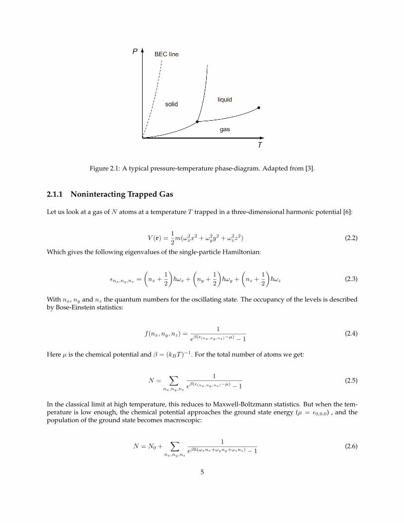
Figure 2.1: A typical pressure-temperature phase-diagram. Adapted from [3].

2.1.1 Noninteracting Trapped Gas

Let us look at a gas of N atoms at a temperature T trapped in a three-dimensional harmonic potential [6]:

V (r) =12m(ω2

xx2 + ω2

yy2 + ω2

zz2) (2.2)

Which gives the following eigenvalues of the single-particle Hamiltonian:

εnx,ny,nz=(nx +

12

)~ωx +

(ny +

12

)~ωy +

(nz +

12

)~ωz (2.3)

With nx, ny and nz the quantum numbers for the oscillating state. The occupancy of the levels is describedby Bose-Einstein statistics:

f(nx, ny, nz) =1

eβ(ε(nx,ny,nz)−µ) − 1(2.4)

Here µ is the chemical potential and β = (kBT )−1. For the total number of atoms we get:

N =∑

nx,ny,nz

1

eβ(ε(nx,ny,nz)−µ) − 1(2.5)

In the classical limit at high temperature, this reduces to Maxwell-Boltzmann statistics. But when the tem-perature is low enough, the chemical potential approaches the ground state energy (µ = ε0,0,0) , and thepopulation of the ground state becomes macroscopic:

N = N0 +∑

nx,ny,nz

1eβ~(ωxnx+ωyny+ωznz) − 1

(2.6)

5

If the level spacing is much smaller than kBT , the sum can be substituted with an integral. We find that thenumber of atoms in the condensate is:

N0 = N

(1−

( TTC

)3) (2.7)

And a critical temperature of:

TC =~ωkB

(N

ζ(3)

)1/3

(2.8)

in which ζ(n) is the Riemann function. For T = 0 all of the atoms will be in the ground state. The density ofthe condensate fraction is then a Gaussian:

n(r) = N

(mω

π~

)3/2

e−m~ (ωxx2+ωyy2+ωzz2) (2.9)

The harmonically trapped gas is much different from a gas in a box, in that the condensation occurs with anarrowing of the density distribution in both the momentum and the coordinate space. In a trapped gas ina box, only the narrowing in the momentum space happens.

2.1.2 The Interacting Trapped Gas

Unfortunately, the ideal situation as described in the previous section can most of the time only be an ap-proximation, since interactions play a big role. Interactions lead to a non-linearity in the de Broglie matter-wave. When strong interactions are present, Bose-Einstein condensation stops being merely a quantumphenomenon and even at zero temperature there will be a significant fraction of the atoms not in the con-densate phase. For weakly interacting gases, this quantum depletion can be ignored.To study systems with strong interactions, we look at the many-body Hamiltonian for a system in potentialVext in the second quantization [6]:

H =∫drΨ†(r)

(− ~2∇2

2m+ Vext(r)

)Ψ(r) (2.10)

+12

∫ ∫drdr′Ψ†(r)Ψ†(r′)Vint(|r− r′|)Ψ(r′)Ψ(r)

Here Ψ is the boson field annihilation operator, Ψ† the boson field creation operator and Vint describes theinteractions between the particles. In a dilute gas, only the s-wave collisions are important.In a general way we can write the field operator in the Heisenberg representation:

Ψ(r, t) = Ψ(r, t) + δΨ(r, t) (2.11)With: Ψ(r, t) = 〈Ψ(r, t)〉 (2.12)

In the Bogoliubov approximation, we neglect δΨ(r, t). This means that the Heisenberg equation of motionbecomes:

i~∂

∂tΨ(r, t) =

(− ~2∇2

2m+ Vext(r) (2.13)

+∫dr′Ψ(r′, t)Vint(r− r′)Ψ(r′, t)

)Ψ(r, t)

6

Where the complex function Ψ(r, t) is the condensate wavefunction. If we satisfy the diluteness condition,so the interparticle distance n−1/3 is much larger than the range of the interaction potential Vint, the equationbecomes:

i~∂

∂tΨ(r, t) =

(− ~2∇2

2m+ Vext + g|Ψ(r, t)|2

)Ψ(r, t) (2.14)

This equation is called the Gross-Piteavskii equation, after the two scientist who independently derived it.The interaction parameter g is:

g =4π~2a

m(2.15)

Here a is the scattering length. As we can see from equation (2.14) the interactions introduce a nonlinearterm in the wave function. Stationary solutions can be found when using the Ansatz:

Ψ(r, t) = e−iµt/~ψ(r) (2.16)

⇒(− ~2∇2

2m+ Vext(r) + g|ψ(r)|2

)ψ(r) = µψ(r) (2.17)

This is the time-independent Gross-Pitaevskii equation. We can calculate the properties of the ground state,for this we use the Thomas-Fermi approximation. We can use this approximation if we have a large numberof atoms and the interaction term dominates the kinetic term, so Na/a0 1 where a0 =

√~/mwho is the

average harmonic oscillator length. This inequality is easily satisfied in most experiments, and gives us adensity distribution:

n(r) = |ψ(r)|2 =1g(µ− Vext(r))θ(µ− Vext(r)) (2.18)

Here θ is the Heaviside function. For a gas in an axially symmetric harmonic trap with ωx = ωy = ω⊥ thisgives us an inverted parabola for the density distribution:

n(r) = n0

(1− x2 + y2

R2⊥

− z2

R2z

)θ

(1− x2 + y2

R2⊥

− z2

R2z

)(2.19)

With height and width:

n0 =µ

g=

~ωho

2g

(15Naaho

)2/5

(2.20)

Rz =

√2µmω2

z

(2.21)

R⊥ =

√2µmω2

⊥(2.22)

2.1.3 The One-Dimensional Bose-Gas

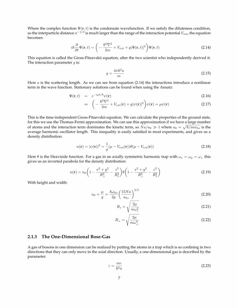
A gas of bosons in one dimension can be realized by putting the atoms in a trap which is so confining in twodirections that they can only move in the axial direction. Usually, a one-dimensional gas is described by theparameter:

γ =mc

~2n(2.23)

7

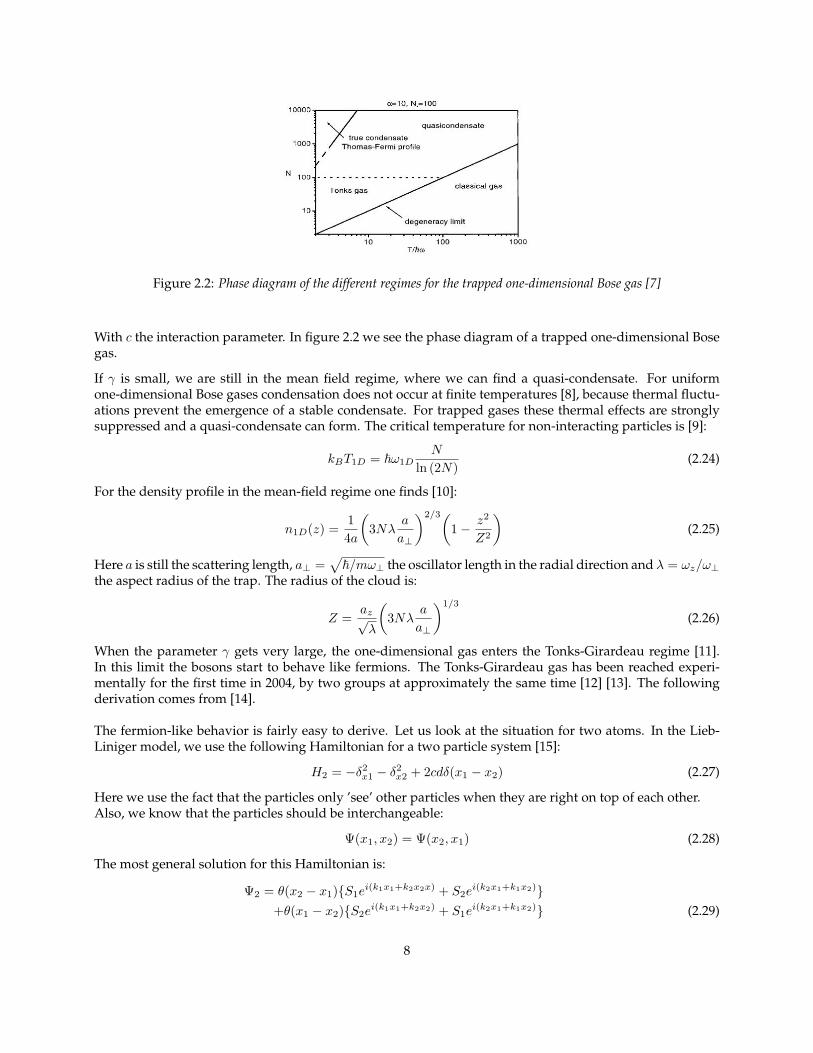
Figure 2.2: Phase diagram of the different regimes for the trapped one-dimensional Bose gas [7]

With c the interaction parameter. In figure 2.2 we see the phase diagram of a trapped one-dimensional Bosegas.

If γ is small, we are still in the mean field regime, where we can find a quasi-condensate. For uniformone-dimensional Bose gases condensation does not occur at finite temperatures [8], because thermal fluctu-ations prevent the emergence of a stable condensate. For trapped gases these thermal effects are stronglysuppressed and a quasi-condensate can form. The critical temperature for non-interacting particles is [9]:

kBT1D = ~ω1DN

ln (2N)(2.24)

For the density profile in the mean-field regime one finds [10]:

n1D(z) =14a

(3Nλ

a

a⊥

)2/3(1− z2

Z2

)(2.25)

Here a is still the scattering length, a⊥ =√

~/mω⊥ the oscillator length in the radial direction and λ = ωz/ω⊥the aspect radius of the trap. The radius of the cloud is:

Z =az√λ

(3Nλ

a

a⊥

)1/3

(2.26)

When the parameter γ gets very large, the one-dimensional gas enters the Tonks-Girardeau regime [11].In this limit the bosons start to behave like fermions. The Tonks-Girardeau gas has been reached experi-mentally for the first time in 2004, by two groups at approximately the same time [12] [13]. The followingderivation comes from [14].

The fermion-like behavior is fairly easy to derive. Let us look at the situation for two atoms. In the Lieb-Liniger model, we use the following Hamiltonian for a two particle system [15]:

H2 = −δ2x1 − δ2x2 + 2cdδ(x1 − x2) (2.27)

Here we use the fact that the particles only ’see’ other particles when they are right on top of each other.Also, we know that the particles should be interchangeable:

Ψ(x1, x2) = Ψ(x2, x1) (2.28)

The most general solution for this Hamiltonian is:

Ψ2 = θ(x2 − x1)S1ei(k1x1+k2x2x) + S2e

i(k2x1+k1x2)+θ(x1 − x2)S2e

i(k1x1+k2x2) + S1ei(k2x1+k1x2) (2.29)

8

Here θ(x2− x1) is the Heaviside function. We can expand this function and after some calculations we find:

H2Ψ2 =(− ∂2

x1− ∂2

x2+ 2cδ(x1 − x2)

)Ψ2

= 2δ(x1 − x2)i(k1 − k2)(S1 − S2)ei(k1+k2)x1+ (k2

1 + k22)Ψ2 + 2cδ(x1 − x2)(S1 + S2)ei(k1+k2)x1 (2.30)

And:2i(k1 − k2)(S1 − S2) + 2c(S1 + S2) = 0 (2.31)

S1(c+ i(k1 − k2)) = S2(c− i(k1 − k2))S2

S1= −c+ i(k1 − k2)

c− i(k1 − k2)= −eiφ(k1,k2) (2.32)

With: φ(k1, k2) =1i

lnc+ i(k1 − k2)c− i(k1 − k2)

= 2 arctank1 − k2

c(2.33)

The limit of c→∞ can be viewed as an ’impenetrable shell’ limit, since this is how the particles behave. Wecan write this behavior as:

Ψ2(x1, . . . , xN ) = 0 als |xj − xl| 5 a (2.34)

When c→∞:

φ(k1, k2) =1i

lnc+ i(k1 − k2)c− i(k1 − k2)

=1i

ln∞+ i(k1 − k2)∞− i(k1 − k2)

= 0

⇒ S2

S1= −1 (2.35)

This points to an isomorphism between free fermions and the gas of bosons with a high c, or high γ. Thesame calculations can be done for more than two particles, the result will be the same.Since the energy and density operators do not distinguish between fermions and bosons, the energy anddensity profiles for the two will be the same. The momentum distribution will be different though, becausethe momentum operator is a Fourier transform of the wave function and therefore does distinguish betweendifferent types of particle.A few theoretical examples of this behavior can be seen in figure 2.3. We can see that with increasinginteraction strength the bosons start to behave as fermions.

2.2 The Cooling and Trapping of Neutral Atoms

Ever since the beginning of experiments working with cold atoms, improvements have been made on howto reach lower and lower temperatures. The first proposal to use lasers to cool atomic samples came fromT.W. Hansch and A.L. Schawlow, who proposed to use the scattering force of the photons to slow down theatoms. When merely looking at the scattering force, there is a fundamental limit one can reach for coolingatoms, the recoil energy TR = ~2k2/mkB , which is the energy an atom gains when absorbing a photon.However, when using lasers to cool neutral atoms, there are ways to reach sub-Doppler temperatures. Thismethod is called Sisyphus cooling, and was one of the reasons for the awarding of the Nobel prize of 1997 toC. Cohen-Tannoudji, S. Chu and W.D. Phillips (They got the prize ’for development of methods to cool andtrap atoms with laser light [18]). With these methods it is possible to get the atoms to∼ 100 nK, which is coldenough for Bose-Einstein condensation, however the densities reached are not sufficient for condensation.

9

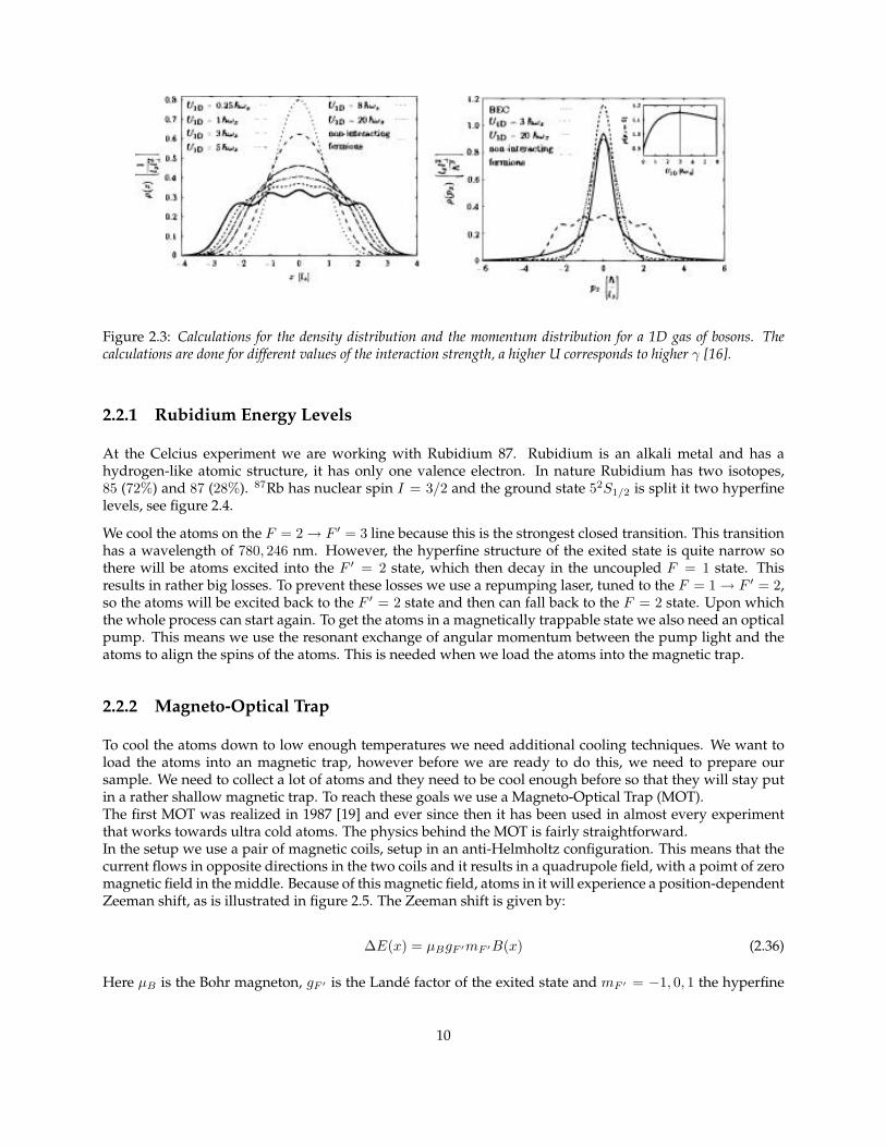
Figure 2.3: Calculations for the density distribution and the momentum distribution for a 1D gas of bosons. Thecalculations are done for different values of the interaction strength, a higher U corresponds to higher γ [16].

2.2.1 Rubidium Energy Levels

At the Celcius experiment we are working with Rubidium 87. Rubidium is an alkali metal and has ahydrogen-like atomic structure, it has only one valence electron. In nature Rubidium has two isotopes,85 (72%) and 87 (28%). 87Rb has nuclear spin I = 3/2 and the ground state 52S1/2 is split it two hyperfinelevels, see figure 2.4.

We cool the atoms on the F = 2 → F ′ = 3 line because this is the strongest closed transition. This transitionhas a wavelength of 780, 246 nm. However, the hyperfine structure of the exited state is quite narrow sothere will be atoms excited into the F ′ = 2 state, which then decay in the uncoupled F = 1 state. Thisresults in rather big losses. To prevent these losses we use a repumping laser, tuned to the F = 1 → F ′ = 2,so the atoms will be excited back to the F ′ = 2 state and then can fall back to the F = 2 state. Upon whichthe whole process can start again. To get the atoms in a magnetically trappable state we also need an opticalpump. This means we use the resonant exchange of angular momentum between the pump light and theatoms to align the spins of the atoms. This is needed when we load the atoms into the magnetic trap.

2.2.2 Magneto-Optical Trap

To cool the atoms down to low enough temperatures we need additional cooling techniques. We want toload the atoms into an magnetic trap, however before we are ready to do this, we need to prepare oursample. We need to collect a lot of atoms and they need to be cool enough before so that they will stay putin a rather shallow magnetic trap. To reach these goals we use a Magneto-Optical Trap (MOT).The first MOT was realized in 1987 [19] and ever since then it has been used in almost every experimentthat works towards ultra cold atoms. The physics behind the MOT is fairly straightforward.In the setup we use a pair of magnetic coils, setup in an anti-Helmholtz configuration. This means that thecurrent flows in opposite directions in the two coils and it results in a quadrupole field, with a poimt of zeromagnetic field in the middle. Because of this magnetic field, atoms in it will experience a position-dependentZeeman shift, as is illustrated in figure 2.5. The Zeeman shift is given by:

∆E(x) = µBgF ′mF ′B(x) (2.36)

Here µB is the Bohr magneton, gF ′ is the Lande factor of the exited state and mF ′ = −1, 0, 1 the hyperfine

10

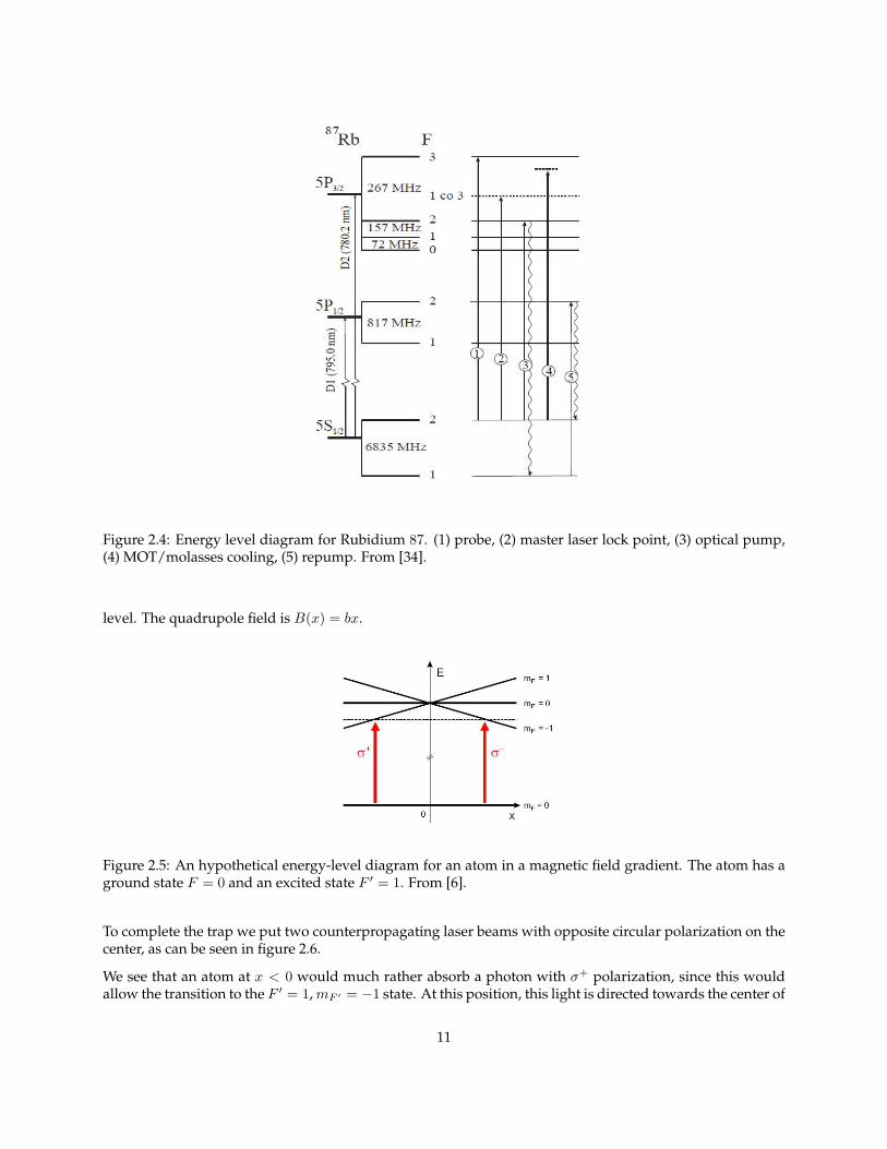
Figure 2.4: Energy level diagram for Rubidium 87. (1) probe, (2) master laser lock point, (3) optical pump,(4) MOT/molasses cooling, (5) repump. From [34].

level. The quadrupole field is B(x) = bx.

Figure 2.5: An hypothetical energy-level diagram for an atom in a magnetic field gradient. The atom has aground state F = 0 and an excited state F ′ = 1. From [6].

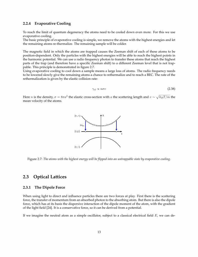
To complete the trap we put two counterpropagating laser beams with opposite circular polarization on thecenter, as can be seen in figure 2.6.

We see that an atom at x < 0 would much rather absorb a photon with σ+ polarization, since this wouldallow the transition to the F ′ = 1,mF ′ = −1 state. At this position, this light is directed towards the center of

11

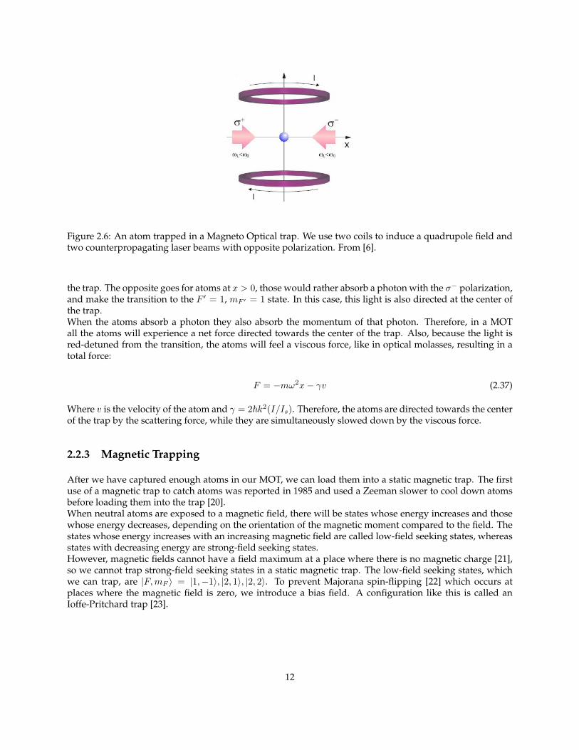
Figure 2.6: An atom trapped in a Magneto Optical trap. We use two coils to induce a quadrupole field andtwo counterpropagating laser beams with opposite polarization. From [6].

the trap. The opposite goes for atoms at x > 0, those would rather absorb a photon with the σ− polarization,and make the transition to the F ′ = 1, mF ′ = 1 state. In this case, this light is also directed at the center ofthe trap.When the atoms absorb a photon they also absorb the momentum of that photon. Therefore, in a MOTall the atoms will experience a net force directed towards the center of the trap. Also, because the light isred-detuned from the transition, the atoms will feel a viscous force, like in optical molasses, resulting in atotal force:

F = −mω2x− γv (2.37)

Where v is the velocity of the atom and γ = 2~k2(I/Is). Therefore, the atoms are directed towards the centerof the trap by the scattering force, while they are simultaneously slowed down by the viscous force.

2.2.3 Magnetic Trapping

After we have captured enough atoms in our MOT, we can load them into a static magnetic trap. The firstuse of a magnetic trap to catch atoms was reported in 1985 and used a Zeeman slower to cool down atomsbefore loading them into the trap [20].When neutral atoms are exposed to a magnetic field, there will be states whose energy increases and thosewhose energy decreases, depending on the orientation of the magnetic moment compared to the field. Thestates whose energy increases with an increasing magnetic field are called low-field seeking states, whereasstates with decreasing energy are strong-field seeking states.However, magnetic fields cannot have a field maximum at a place where there is no magnetic charge [21],so we cannot trap strong-field seeking states in a static magnetic trap. The low-field seeking states, whichwe can trap, are |F,mF 〉 = |1,−1〉, |2, 1〉, |2, 2〉. To prevent Majorana spin-flipping [22] which occurs atplaces where the magnetic field is zero, we introduce a bias field. A configuration like this is called anIoffe-Pritchard trap [23].

12

2.2.4 Evaporative Cooling

To reach the limit of quantum degeneracy the atoms need to be cooled down even more. For this we useevaporative cooling.The basic principle of evaporative cooling is simple, we remove the atoms with the highest energies and letthe remaining atoms re-thermalize. The remaining sample will be colder.

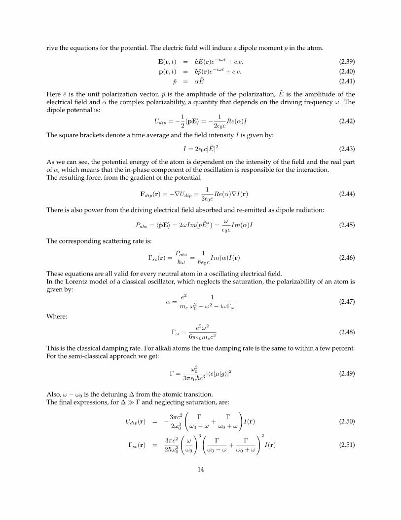
The magnetic field in which the atoms are trapped causes the Zeeman shift of each of these atoms to beposition-dependent. Only the particles with the highest energies will be able to reach the highest points inthe harmonic potential. We can use a radio frequency photon to transfer these atoms that reach the highestparts of the trap (and therefore have a specific Zeeman shift) to a different Zeeman level that is not trap-pable. This principle is demonstrated in figure 2.7.Using evaporative cooling to cool down a sample means a large loss of atoms. The radio frequency needsto be lowered slowly give the remaining atoms a chance to rethermalize and to reach a BEC. The rate of therethermalization is given by the elastic collision rate:

γel ∝ nσv (2.38)

Here n is the density, σ = 8πa2 the elastic cross-section with a the scattering length and v ∼√kBT/m the

mean velocity of the atoms.

Figure 2.7: The atoms with the highest energy will be flipped into an untrappable state by evaporative cooling.

2.3 Optical Lattices

2.3.1 The Dipole Force

When using light to direct and influence particles there are two forces at play. First there is the scatteringforce, the transfer of momentum from an absorbed photon to the absorbing atom. But there is also the dipoleforce, which has at its basis the dispersive interaction of the dipole moment of the atom, with the gradientof the light field [24]. It is a conservative force, so it can be derived from a potential.

If we imagine the neutral atom as a simple oscillator, subject to a classical electrical field E, we can de-

13

rive the equations for the potential. The electric field will induce a dipole moment p in the atom.

E(r, t) = eE(r)e−iωt + c.c. (2.39)p(r, t) = ep(r)e−iωt + c.c. (2.40)

p = αE (2.41)

Here e is the unit polarization vector, p is the amplitude of the polarization, E is the amplitude of theelectrical field and α the complex polarizability, a quantity that depends on the driving frequency ω. Thedipole potential is:

Udip = −12〈pE〉 = − 1

2ε0cRe(α)I (2.42)

The square brackets denote a time average and the field intensity I is given by:

I = 2ε0c|E|2 (2.43)

As we can see, the potential energy of the atom is dependent on the intensity of the field and the real partof α, which means that the in-phase component of the oscillation is responsible for the interaction.The resulting force, from the gradient of the potential:

Fdip(r) = −∇Udip =1

2ε0cRe(α)∇I(r) (2.44)

There is also power from the driving electrical field absorbed and re-emitted as dipole radiation:

Pabs = 〈pE〉 = 2ωIm(pE∗) =ω

ε0cIm(α)I (2.45)

The corresponding scattering rate is:

Γsc(r) =Pabs

~ω=

1~ε0c

Im(α)I(r) (2.46)

These equations are all valid for every neutral atom in a oscillating electrical field.In the Lorentz model of a classical oscillator, which neglects the saturation, the polarizability of an atom isgiven by:

α =e2

me

1ω2

0 − ω2 − iωΓω(2.47)

Where:

Γω =e2ω2

6πε0mec3(2.48)

This is the classical damping rate. For alkali atoms the true damping rate is the same to within a few percent.For the semi-classical approach we get:

Γ =ω3

0

3πε0~c3|〈e|µ|g〉|2 (2.49)

Also, ω − ω0 is the detuning ∆ from the atomic transition.The final expressions, for ∆ Γ and neglecting saturation, are:

Udip(r) = −3πc2

2ω30

(Γ

ω0 − ω+

Γω0 + ω

)I(r) (2.50)

Γsc(r) =3πc2

2~ω30

(ω

ω0

)3(Γ

ω0 − ω+

Γω0 + ω

)2

I(r) (2.51)

14

If we look at large detuning (∆ Γ) we can simplify these equations, by using the rotating wave approxi-mation (neglecting terms proportional to Γ/(ω0 + ω)), and we see that the potential scales with 1/∆ and thescattering rate with 1/∆2:

Udip(r) =3πc2

2ω30

Γ∆I(r) (2.52)

Γsc(r) =3πc2

2~ω30

(Γ∆

)2

I(r) (2.53)

For detunings smaller than the natural linewidth Γ the strength of the trap drops again and these equationsare not valid anymore.As we see, the sign of the potential depends on the sign of the detuning. If the light is red-detuned (∆ < 0)the potential is negative and atoms will therefore be attracted to the light field. If the light is blue-detunedwith respect to the atomic transition (∆ > 0) the atom will be repelled by the light field. This means thatatoms will seek out the highest intensity in a red-detuned beam and the lowest intensity in a blue-detunedbeam.

2.3.2 The Periodic Potential

In our setup we have two counterpropagating beams, which results in a standing wave of light, thus creatinga periodic potential for the trapped atoms. The theory for particles in periodic potentials has first beendeveloped for electrons in solids, but the principle is the same for our case.

A particle in a Periodic Potential

The simplest case of a periodic potential is a pure sinusoidal potential:

V (x) =V0

2(1− cos 2kx) (2.54)

This potential is periodic so we can write:

V (x) = V (x+ d) (2.55)

Here d = π/k is the lattice spacing, for a standing wave made of light beams, this is half the wavelength ofthe light. For a particle with mass m we have the time-independent single-particle Hamiltonian:

HΨ(x)(− ~2

2m∂2

∂x2+ V (x)

)Ψ(x) = EΨ(x) (2.56)

To solve this equation we need the Bloch Theorem [25], which tells us that the solutions take the form:

Ψn,q(x)eiqxun,q (2.57)un,q(x) = un,q(x+ d) (2.58)

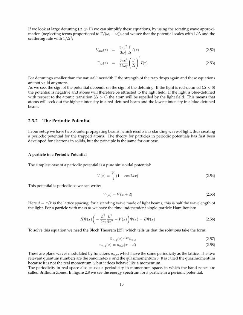
These are plane waves modulated by functions un,q, which have the same periodicity as the lattice. The tworelevant quantum numbers are the band index n and the quasimomentum q. It is called the quasimomentumbecause it is not the real momentum p, but it does behave like a momentum.The periodicity in real space also causes a periodicity in momentum space, in which the band zones arecalled Brillouin Zones. In figure 2.8 we see the energy spectrum for a particle in a periodic potential.

15

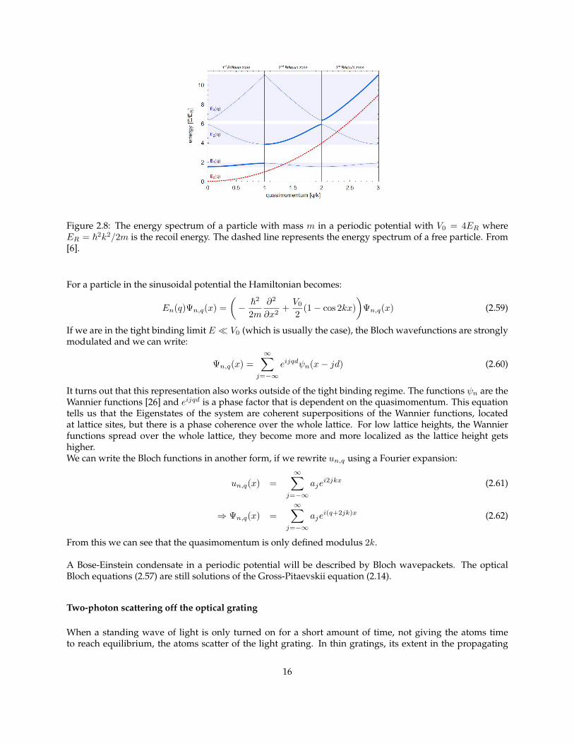
Figure 2.8: The energy spectrum of a particle with mass m in a periodic potential with V0 = 4ER whereER = ~2k2/2m is the recoil energy. The dashed line represents the energy spectrum of a free particle. From[6].

For a particle in the sinusoidal potential the Hamiltonian becomes:

En(q)Ψn,q(x) =(− ~2

2m∂2

∂x2+V0

2(1− cos 2kx)

)Ψn,q(x) (2.59)

If we are in the tight binding limit E V0 (which is usually the case), the Bloch wavefunctions are stronglymodulated and we can write:

Ψn,q(x) =∞∑

j=−∞eijqdψn(x− jd) (2.60)

It turns out that this representation also works outside of the tight binding regime. The functions ψn are theWannier functions [26] and eijqd is a phase factor that is dependent on the quasimomentum. This equationtells us that the Eigenstates of the system are coherent superpositions of the Wannier functions, locatedat lattice sites, but there is a phase coherence over the whole lattice. For low lattice heights, the Wannierfunctions spread over the whole lattice, they become more and more localized as the lattice height getshigher.We can write the Bloch functions in another form, if we rewrite un,q using a Fourier expansion:

un,q(x) =∞∑

j=−∞aje

i2jkx (2.61)

⇒ Ψn,q(x) =∞∑

j=−∞aje

i(q+2jk)x (2.62)

From this we can see that the quasimomentum is only defined modulus 2k.

A Bose-Einstein condensate in a periodic potential will be described by Bloch wavepackets. The opticalBloch equations (2.57) are still solutions of the Gross-Pitaevskii equation (2.14).

Two-photon scattering off the optical grating

When a standing wave of light is only turned on for a short amount of time, not giving the atoms timeto reach equilibrium, the atoms scatter of the light grating. In thin gratings, its extent in the propagating

16

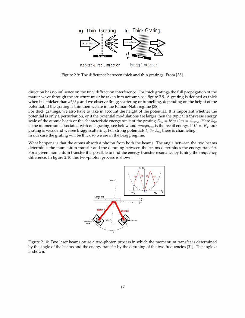
Figure 2.9: The difference between thick and thin gratings. From [38].

direction has no influence on the final diffraction interference. For thick gratings the full propagation of thematter-wave through the structure must be taken into account, see figure 2.9. A grating is defined as thickwhen it is thicker than d2/λB and we observe Bragg scattering or tunnelling, depending on the height of thepotential. If the grating is thin then we are in the Raman-Nath regime [38].For thick gratings, we also have to take in account the height of the potential. It is important whether thepotential is only a perturbation, or if the potential modulations are larger then the typical transverse energyscale of the atomic beam or the characteristic energy scale of the grating Eq0 = ~2q20/2m = 4ωrec. Here ~q0is the momentum associated with one grating, see below and omegarec is the recoil energy. If U Eq0 ourgrating is weak and we see Bragg scattering. For strong potentials U Eq0 there is channeling.In our case the grating will be thick so we are in the Bragg regime.

What happens is that the atoms absorb a photon from both the beams. The angle between the two beamsdetermines the momentum transfer and the detuning between the beams determines the energy transfer.For a given momentum transfer it is possible to find the energy transfer resonance by tuning the frequencydifference. In figure 2.10 this two-photon process is shown.

Figure 2.10: Two laser beams cause a two-photon process in which the momentum transfer is determinedby the angle of the beams and the energy transfer by the detuning of the two frequencies [31]. The angle αis shown.

17

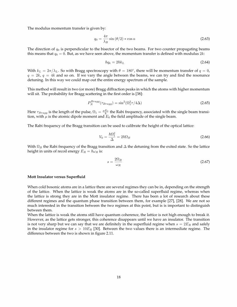
The modulus momentum transfer is given by:

q0 =4πλB

sin (θ/2) ∗ cosα (2.63)

The direction of q0 is perpendicular to the bisector of the two beams. For two counter propagating beamsthis means that q0 = 0. But, as we have seen above, the momentum transfer is defined with modulus 2k:

~qk = 2~kL (2.64)

With kL = 2π/λL. So with Bragg spectroscopy with θ = 180, there will be momentum transfer of q = 0,q = 2k, q = 4k and so on. If we vary the angle between the beams, we can try and find the resonancedetuning. In this way we could map out the entire energy spectrum of the sample.

This method will result in two (or more) Bragg diffraction peaks in which the atoms with higher momentumwill sit. The probability for Bragg scattering in the first order is [38]:

PBraggN (τBragg) = sin2(Ω2

1τ/4∆) (2.65)

Here τBragg is the length of the pulse, Ω1 = µE0~ the Rabi frequency, associated with the single beam transi-

tion, with µ is the atomic dipole moment and E0 the field amplitude of the single beam.

The Rabi frequency of the Bragg transition can be used to calibrate the height of the optical lattice:

V0 =~Ω2

1

∆= 2~ΩB (2.66)

With ΩB the Rabi frequency of the Bragg transition and ∆ the detuning from the exited state. So the latticeheight in units of recoil energy ER = ~ωR is:

s =2ΩB

ωR(2.67)

Mott Insulator versus Superfluid

When cold bosonic atoms are in a lattice there are several regimes they can be in, depending on the strengthof the lattice. When the lattice is weak the atoms are in the so-called superfluid regime, whereas whenthe lattice is strong they are in the Mott insulator regime. There has been a lot of research about thesedifferent regimes and the quantum phase transition between them, for example [27], [28]. We are not somuch interested in the transition between the two regimes at this point, but is is important to distinguishbetween them.When the lattice is weak the atoms still have quantum coherence, the lattice is not high enough to break it.However, as the lattice gets stronger, this coherence disappears until we have an insulator. The transitionis not very sharp but we can say that we are definitely in the superfluid regime when s = 2ER and safelyin the insulator regime for s > 10ER [30]. Between the two values there is an intermediate regime. Thedifference between the two is shown in figure 2.11.

18

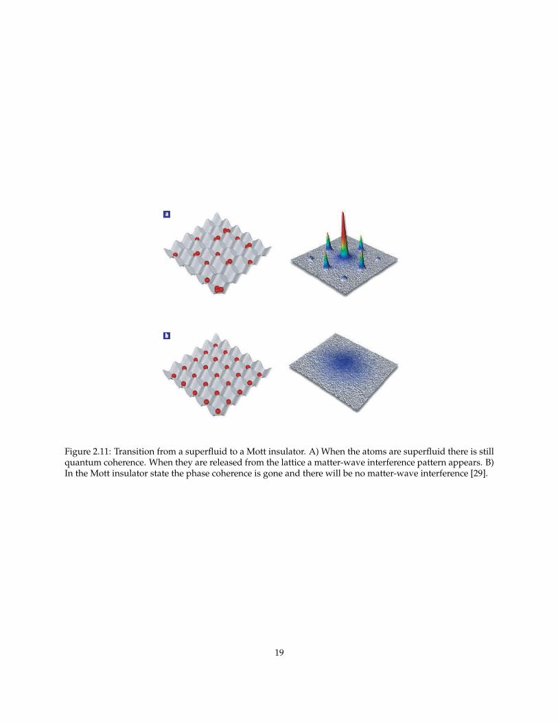
Figure 2.11: Transition from a superfluid to a Mott insulator. A) When the atoms are superfluid there is stillquantum coherence. When they are released from the lattice a matter-wave interference pattern appears. B)In the Mott insulator state the phase coherence is gone and there will be no matter-wave interference [29].

19

Chapter 3

Getting started: building aninterferometer

3.1 Introduction

For an optical lattice we need two counter-propagating beams which will create a standing wave of light.To get a feeling for how such a systems works, we decided to first build everything separate from theexperiment. In this controlled environment we can do all the stability measurements we want to do andeasily make changes to the setup, if necessary.Because we have this setup with the two beams, a good way to study it is building an interferometer. Weare mostly interested in the stability, since if we want to use the setup as an optical lattice, it needs to bestable on the order of wavelengths.

3.2 The Theory Behind Interferometers

Interferometers have been around for some time. They are a perfect apparatus to study the differencebetween light beams or the medium the light is travelling trough. Michelson and Morley used an interfer-ometer in their search for the ether [32], this type of setup is still widely used.

Interferometers work on the principle of interference. This is the superposition of two waves. These wavescan interact either constructively or destructively, depending on the relative position of their nodes and anti-nodes, see figure 3.1. Note that the nature of these waves in no way restricted to light waves. Interferencefor example also occurs in sound waves or in matter waves [33].When working with light interference there is one more aspect to worry about, which is the polarizationof the light. Coherent laser beams will have a definitive polarization. If one of the two beams picks up achange in its polarization, this will effect the interference pattern. Only light with the same polarizationcan interfere. So if the beams have complete orthogonal polarization, there will be no interference effect.However, if there is only a slight difference in polarization, the parts that are polarized in the same directionwill still interfere. However, the contrast will not be complete anymore.

An interferometer usually looks at two waves which are recombined after having taken separate and differ-ent paths see figure 3.2. When they are recombined, the waves interfere in a way that is depending on theirrelative phase. Their relative phase can be determined by what happened to the beams while they where

20

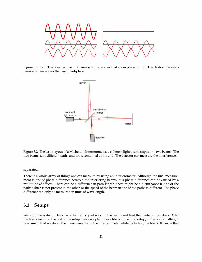
Figure 3.1: Left: The constructive interference of two waves that are in phase. Right: The destructive inter-ference of two waves that are in antiphase.

Figure 3.2: The basic layout of a Michelson Interferometer, a coherent light beam is split into two beams. Thetwo beams take different paths and are recombined at the end. The detector can measure the interference.

separated.

There is a whole array of things one can measure by using an interferometer. Although the final measure-ment is one of phase difference between the interfering beams, this phase difference can be caused by amultitude of effects. There can be a difference in path length, there might be a disturbance in one of thepaths which is not present in the other, or the speed of the beam in one of the paths is different. The phasedifference can only be measured in units of wavelength.

3.3 Setups

We build the system in two parts. In the first part we split the beams and feed them into optical fibers. Afterthe fibers we build the rest of the setup. Since we plan to use fibers in the final setup, in the optical lattice, itis adamant that we do all the measurements on the interferometer while including the fibers. It can be that

21

something happens while the light is inside the fibers which messes with its properties.

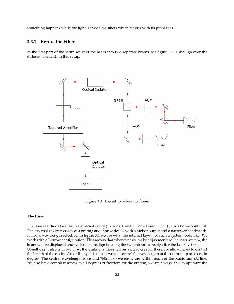
3.3.1 Before the Fibers

In the first part of the setup we split the beam into two separate beams, see figure 3.3. I shall go over thedifferent elements in this setup.

Figure 3.3: The setup before the fibers

The Laser

The laser is a diode laser with a external cavity (External Cavity Diode Laser, ECDL) , it is a home built unit.The external cavity consists of a grating and it provides us with a higher output and a narrower bandwidth.It also is wavelength selective. In figure 3.4 we see what the internal layout of such a system looks like. Wework with a Littrow configuration. This means that whenever we make adjustments to the laser system, thebeam will be displaced and we have to realign it, using the two mirrors directly after the laser system.Usually, as it also is in our case, the grating is mounted on a piezo crystal, therefore allowing us to controlthe length of the cavity. Accordingly, this means we can control the wavelength of the output, up to a certaindegree. The central wavelength is around 780nm so we easily are within reach of the Rubidium D2 line.We also have complete access to all degrees of freedom for the grating, we are always able to optimize the

22

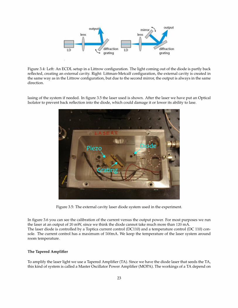
Figure 3.4: Left: An ECDL setup in a Littrow configuration. The light coming out of the diode is partly backreflected, creating an external cavity. Right: Littman-Metcalf configuration, the external cavity is created inthe same way as in the Littrow configuration, but due to the second mirror, the output is always in the samedirection.

lasing of the system if needed. In figure 3.5 the laser used is shown. After the laser we have put an OpticalIsolator to prevent back reflection into the diode, which could damage it or lower its ability to lase.

Figure 3.5: The external cavity laser diode system used in the experiment.

In figure 3.6 you can see the calibration of the current versus the output power. For most purposes we runthe laser at an output of 20 mW, since we think the diode cannot take much more than 120 mA.The laser diode is controlled by a Toptica current control (DC110) and a temperature control (DC 110) con-sole. The current control has a maximum of 500mA. We keep the temperature of the laser system aroundroom temperature.

The Tapered Amplifier

To amplify the laser light we use a Tapered Amplifier (TA). Since we have the diode laser that seeds the TA,this kind of system is called a Master Oscillator Power Amplifier (MOPA). The workings of a TA depend on

23

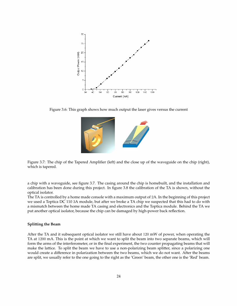
Figure 3.6: This graph shows how much output the laser gives versus the current

Figure 3.7: The chip of the Tapered Amplifier (left) and the close up of the waveguide on the chip (right),which is tapered.

a chip with a waveguide, see figure 3.7. The casing around the chip is homebuilt, and the installation andcalibration has been done during this project. In figure 3.8 the calibration of the TA is shown, without theoptical isolator.The TA is controlled by a home made console with a maximum output of 2A. In the beginning of this projectwe used a Toptica DC 110 3A module, but after we broke a TA chip we suspected that this had to do witha mismatch between the home made TA casing and electronics and the Toptica module. Behind the TA weput another optical isolator, because the chip can be damaged by high-power back reflection.

Splitting the Beam

After the TA and it subsequent optical isolator we still have about 120 mW of power, when operating theTA at 1200 mA. This is the point at which we want to split the beam into two separate beams, which willform the arms of the interferometer, or in the final experiment, the two counter propagating beams that willmake the lattice. To split the beam we have to use a non-polarizing beam splitter, since a polarizing onewould create a difference in polarization between the two beams, which we do not want. After the beamsare split, we usually refer to the one going to the right as the ’Green’ beam, the other one is the ’Red’ beam.

24

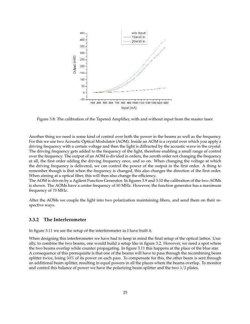
Figure 3.8: The calibration of the Tapered Amplifier, with and without input from the master laser.

Another thing we need is some kind of control over both the power in the beams as well as the frequency.For this we use two Acoustic Optical Modulator (AOM). Inside an AOM is a crystal over which you apply adriving frequency with a certain voltage and then the light is diffracted by the acoustic wave in the crystal.The driving frequency gets added to the frequency of the light, therefore enabling a small range of controlover the frequency. The output of an AOM is divided in orders, the zeroth order not changing the frequencyat all, the first order adding the driving frequency once, and so on. When changing the voltage at whichthe driving frequency is delivered, we can control the power of the output in the first order. A thing toremember though is that when the frequency is changed, this also changes the direction of the first order.When aiming at a optical fiber, this will then also change the efficiency.The AOM is driven by a Agilent Function Generator. In figures 3.9 and 3.10 the calibration of the two AOMsis shown. The AOMs have a center frequency of 80 MHz. However, the function generator has a maximumfrequency of 79 MHz.

After the AOMs we couple the light into two polarization maintaining fibers, and send them on their re-spective ways.

3.3.2 The Interferometer

In figure 3.11 we see the setup of the interferometer as I have built it.

When designing this interferometer we have had to keep in mind the final setup of the optical lattice. Usu-ally, to combine the two beams, one would build a setup like in figure 3.2. However, we need a spot wherethe two beams overlap while counter propagating. In figure 3.11 this happens at the place of the blue star.A consequence of this prerequisite is that one of the beams will have to pass through the recombining beamsplitter twice, losing 50% of its power on each pass. To compensate for this, the other beam is sent throughan additional beam splitter, resulting in equal powers in all the places where the beams overlap. To monitorand control this balance of power we have the polarizing beam splitter and the two λ/2 plates.

25

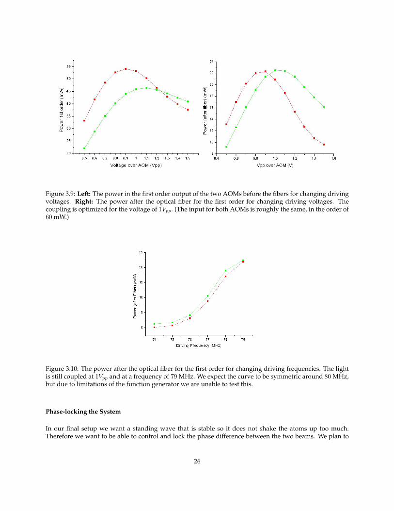
Figure 3.9: Left: The power in the first order output of the two AOMs before the fibers for changing drivingvoltages. Right: The power after the optical fiber for the first order for changing driving voltages. Thecoupling is optimized for the voltage of 1Vpp. (The input for both AOMs is roughly the same, in the order of60 mW.)

Figure 3.10: The power after the optical fiber for the first order for changing driving frequencies. The lightis still coupled at 1Vpp and at a frequency of 79 MHz. We expect the curve to be symmetric around 80 MHz,but due to limitations of the function generator we are unable to test this.

Phase-locking the System

In our final setup we want a standing wave that is stable so it does not shake the atoms up too much.Therefore we want to be able to control and lock the phase difference between the two beams. We plan to

26

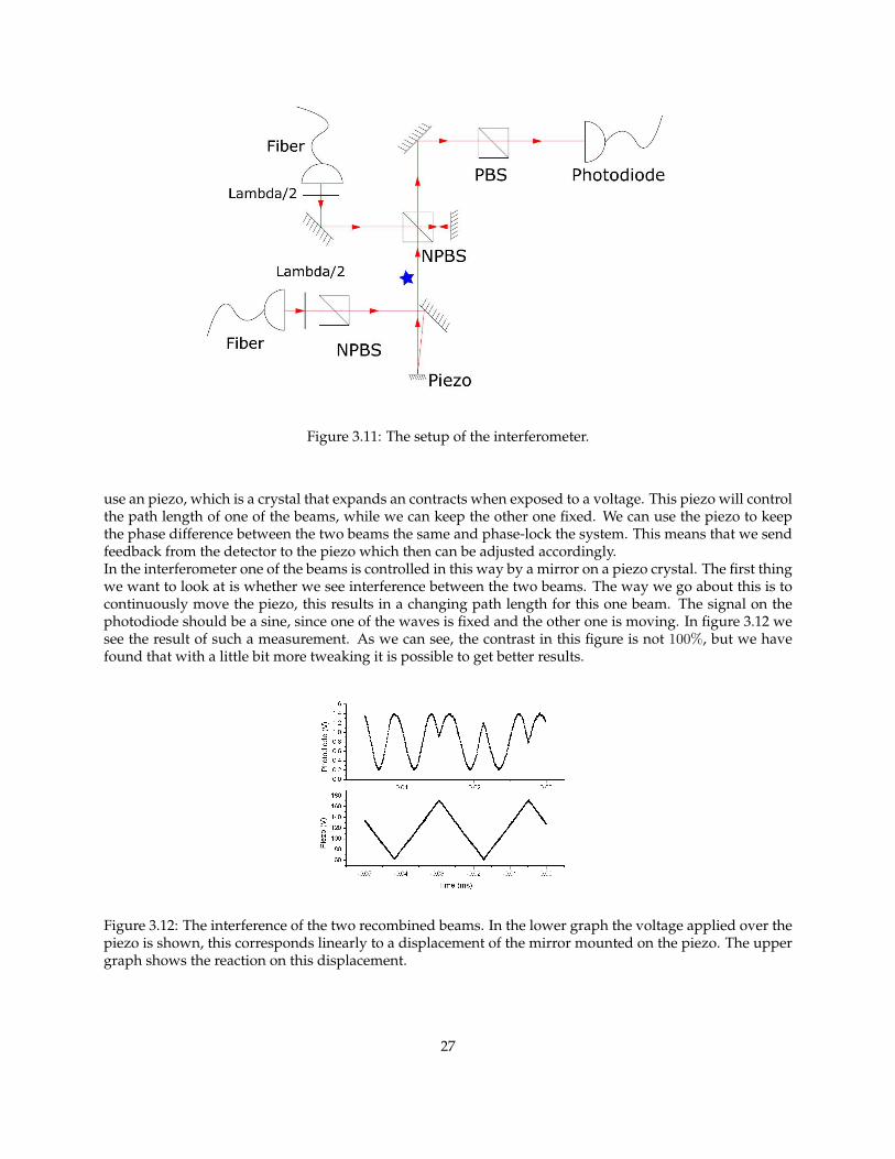
Figure 3.11: The setup of the interferometer.

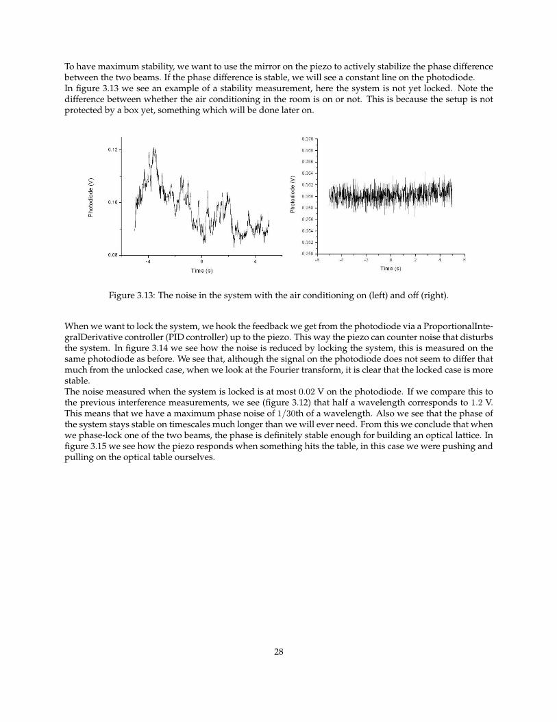
use an piezo, which is a crystal that expands an contracts when exposed to a voltage. This piezo will controlthe path length of one of the beams, while we can keep the other one fixed. We can use the piezo to keepthe phase difference between the two beams the same and phase-lock the system. This means that we sendfeedback from the detector to the piezo which then can be adjusted accordingly.In the interferometer one of the beams is controlled in this way by a mirror on a piezo crystal. The first thingwe want to look at is whether we see interference between the two beams. The way we go about this is tocontinuously move the piezo, this results in a changing path length for this one beam. The signal on thephotodiode should be a sine, since one of the waves is fixed and the other one is moving. In figure 3.12 wesee the result of such a measurement. As we can see, the contrast in this figure is not 100%, but we havefound that with a little bit more tweaking it is possible to get better results.

Figure 3.12: The interference of the two recombined beams. In the lower graph the voltage applied over thepiezo is shown, this corresponds linearly to a displacement of the mirror mounted on the piezo. The uppergraph shows the reaction on this displacement.

27

To have maximum stability, we want to use the mirror on the piezo to actively stabilize the phase differencebetween the two beams. If the phase difference is stable, we will see a constant line on the photodiode.In figure 3.13 we see an example of a stability measurement, here the system is not yet locked. Note thedifference between whether the air conditioning in the room is on or not. This is because the setup is notprotected by a box yet, something which will be done later on.

Figure 3.13: The noise in the system with the air conditioning on (left) and off (right).

When we want to lock the system, we hook the feedback we get from the photodiode via a ProportionalInte-gralDerivative controller (PID controller) up to the piezo. This way the piezo can counter noise that disturbsthe system. In figure 3.14 we see how the noise is reduced by locking the system, this is measured on thesame photodiode as before. We see that, although the signal on the photodiode does not seem to differ thatmuch from the unlocked case, when we look at the Fourier transform, it is clear that the locked case is morestable.The noise measured when the system is locked is at most 0.02 V on the photodiode. If we compare this tothe previous interference measurements, we see (figure 3.12) that half a wavelength corresponds to 1.2 V.This means that we have a maximum phase noise of 1/30th of a wavelength. Also we see that the phase ofthe system stays stable on timescales much longer than we will ever need. From this we conclude that whenwe phase-lock one of the two beams, the phase is definitely stable enough for building an optical lattice. Infigure 3.15 we see how the piezo responds when something hits the table, in this case we were pushing andpulling on the optical table ourselves.

28

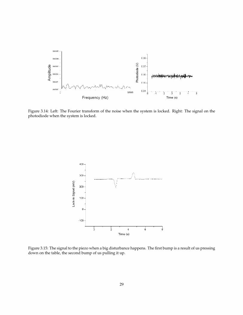
Figure 3.14: Left: The Fourier transform of the noise when the system is locked. Right: The signal on thephotodiode when the system is locked.

Figure 3.15: The signal to the piezo when a big disturbance happens. The first bump is a result of us pressingdown on the table, the second bump of us pulling it up.

29

Chapter 4

The Experiment

4.1 Introduction

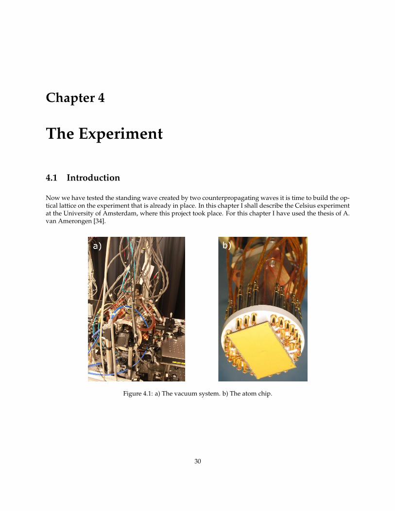
Now we have tested the standing wave created by two counterpropagating waves it is time to build the op-tical lattice on the experiment that is already in place. In this chapter I shall describe the Celsius experimentat the University of Amsterdam, where this project took place. For this chapter I have used the thesis of A.van Amerongen [34].

Figure 4.1: a) The vacuum system. b) The atom chip.

30

Figure 4.2: Schematic drawing of the mirror MOT. The beam in the other direction is not shown. Thequadrupole are shown in black.

4.2 The Celsius Experiment

At the Celcius experiment at the University of Amsterdam we work with ultra cold 87Rb on an atom chip.On the atom chips there are miniwires which we can use to create the necessary confinements. I shall nowquickly describe how we cool, trap and detect the atoms. In figure 4.1 a photo of the vacuumsystem and thechip is shown.

4.2.1 Laser Cooling

The methods used to cool atoms have been described in chapter 2. I shall go over the experimental realiza-tion of these methods in our laboratory briefly.

For cooling the atoms down to a BEC, we first need to get them into a MOT. Since we do not have opticalaccess in all three dimensions (the chip is blocking access from above), we use a mirror MOT, a techniquefirst introduced by Reichel et al in 2001 [37]. A mirror MOT works the same as a conventional MOT system,only one of the beams is reflected of a surface, see figure 4.2. The polarization of the MOT light switcheshandedness when it is reflected off the chip, therefore maintaining the needed polarization for the trap.

We load this trap from the background gas. As a source for Rubidium we use a dispenser that releasesatoms when heated. On a chip, condensates can be produced faster than in conventional traps. The lifetimeof our condensate therefore does not have to be very long (∼ 1 s), and we do not have to move our conden-sate into a separate science chamber with a lower background pressure, as many experiments do.

For cooling the atoms we only need three lasers, a master cooling laser, a slave laser for the master laserthat is locked by injection and a repumper laser. The master laser is a grating stabilized Toptica DL100 laser,that operates near theD2 line, near 780 nm. It has an output of∼ 90 mW and is FM locked on the cross-over(co) line of the F = 2 → F ′ = 1 and the F = 2 → F ′ = 3 transitions.The slave laser is injected with 2 mW of frequency shifted light and produces about 120 mW. This light isthen used for the cooling and probing. The light of the master laser that is not used for injecting the slave,is used for the pump, see figure 2.4. In figure 4.3 the setup of the master-slave laser system is shown. Later,an additional tapered amplifier was introduced for the cooling light.

The repump laser is locked to the F = 1 → F ′ = 2 transition of the D1 line, at 795 nm. It is a grating-

31

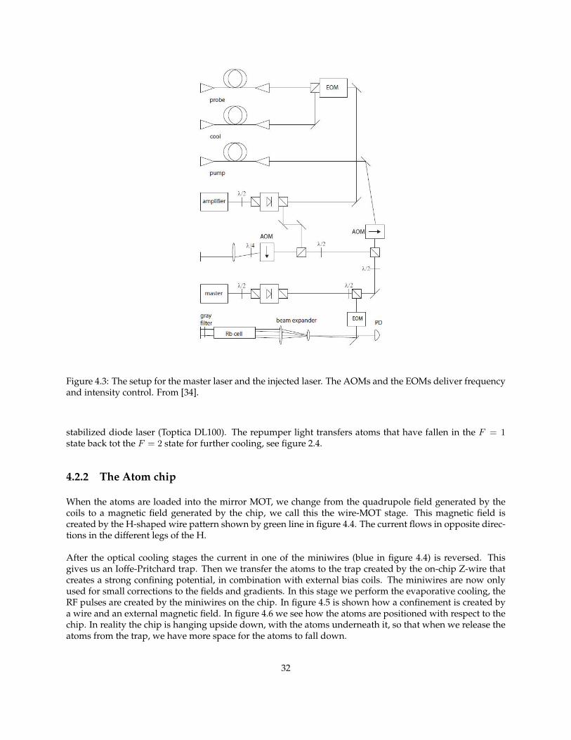
Figure 4.3: The setup for the master laser and the injected laser. The AOMs and the EOMs deliver frequencyand intensity control. From [34].

stabilized diode laser (Toptica DL100). The repumper light transfers atoms that have fallen in the F = 1state back tot the F = 2 state for further cooling, see figure 2.4.

4.2.2 The Atom chip

When the atoms are loaded into the mirror MOT, we change from the quadrupole field generated by thecoils to a magnetic field generated by the chip, we call this the wire-MOT stage. This magnetic field iscreated by the H-shaped wire pattern shown by green line in figure 4.4. The current flows in opposite direc-tions in the different legs of the H.

After the optical cooling stages the current in one of the miniwires (blue in figure 4.4) is reversed. Thisgives us an Ioffe-Pritchard trap. Then we transfer the atoms to the trap created by the on-chip Z-wire thatcreates a strong confining potential, in combination with external bias coils. The miniwires are now onlyused for small corrections to the fields and gradients. In this stage we perform the evaporative cooling, theRF pulses are created by the miniwires on the chip. In figure 4.5 is shown how a confinement is created bya wire and an external magnetic field. In figure 4.6 we see how the atoms are positioned with respect to thechip. In reality the chip is hanging upside down, with the atoms underneath it, so that when we release theatoms from the trap, we have more space for the atoms to fall down.

32

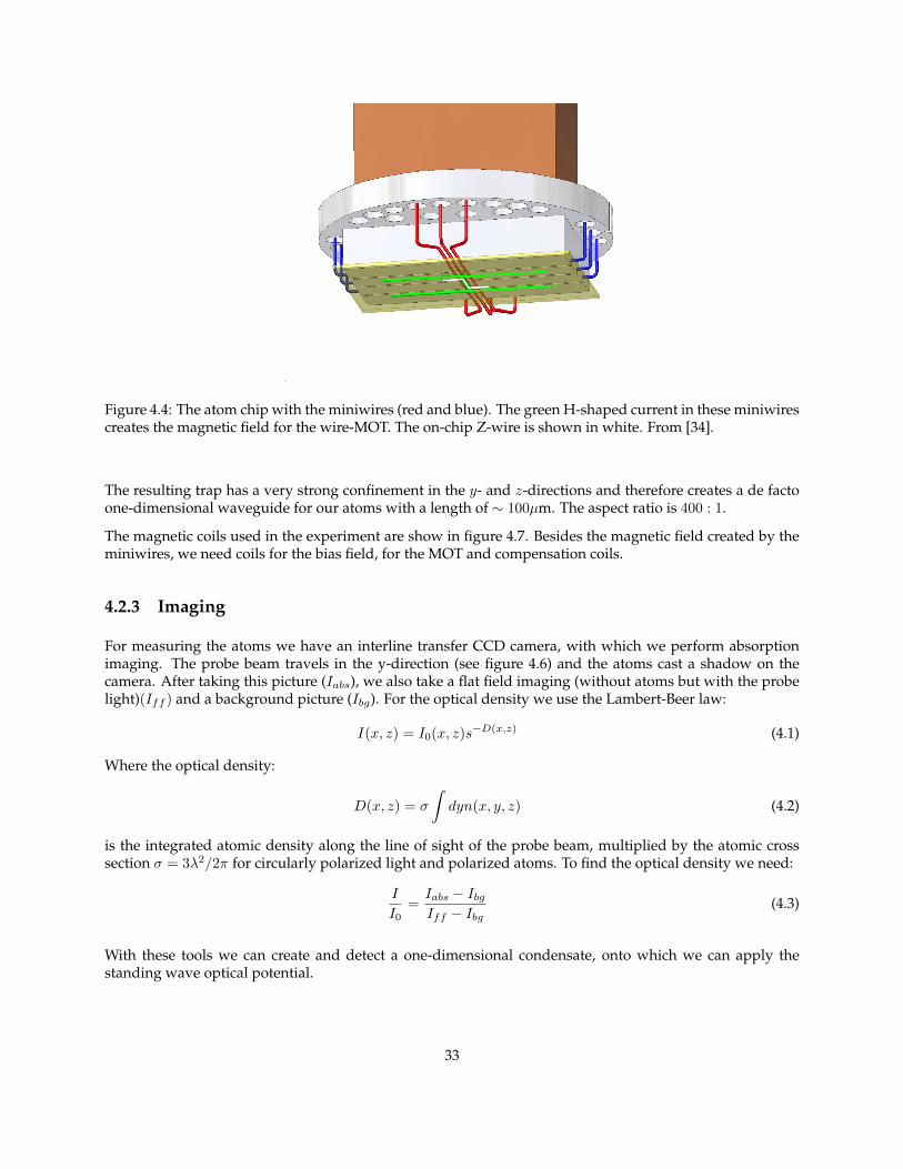
Figure 4.4: The atom chip with the miniwires (red and blue). The green H-shaped current in these miniwirescreates the magnetic field for the wire-MOT. The on-chip Z-wire is shown in white. From [34].

The resulting trap has a very strong confinement in the y- and z-directions and therefore creates a de factoone-dimensional waveguide for our atoms with a length of ∼ 100µm. The aspect ratio is 400 : 1.

The magnetic coils used in the experiment are show in figure 4.7. Besides the magnetic field created by theminiwires, we need coils for the bias field, for the MOT and compensation coils.

4.2.3 Imaging

For measuring the atoms we have an interline transfer CCD camera, with which we perform absorptionimaging. The probe beam travels in the y-direction (see figure 4.6) and the atoms cast a shadow on thecamera. After taking this picture (Iabs), we also take a flat field imaging (without atoms but with the probelight)(Iff ) and a background picture (Ibg). For the optical density we use the Lambert-Beer law:

I(x, z) = I0(x, z)s−D(x,z) (4.1)

Where the optical density:

D(x, z) = σ

∫dyn(x, y, z) (4.2)

is the integrated atomic density along the line of sight of the probe beam, multiplied by the atomic crosssection σ = 3λ2/2π for circularly polarized light and polarized atoms. To find the optical density we need:

I

I0=Iabs − Ibg

Iff − Ibg(4.3)

With these tools we can create and detect a one-dimensional condensate, onto which we can apply thestanding wave optical potential.

33

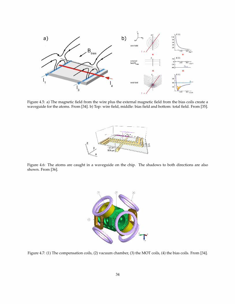
Figure 4.5: a) The magnetic field from the wire plus the external magnetic field from the bias coils create awaveguide for the atoms. From [34]. b) Top: wire field, middle: bias field and bottom: total field. From [35].

Figure 4.6: The atoms are caught in a waveguide on the chip. The shadows to both directions are alsoshown. From [36].

Figure 4.7: (1) The compensation coils, (2) vacuum chamber, (3) the MOT coils, (4) the bias coils. From [34].

34

Chapter 5

The Optical Lattice

5.1 The Optical Lattice

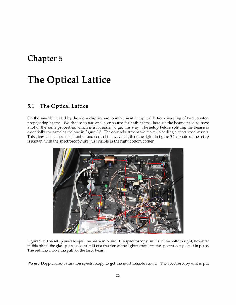
On the sample created by the atom chip we are to implement an optical lattice consisting of two counter-propagating beams. We choose to use one laser source for both beams, because the beams need to havea lot of the same properties, which is a lot easier to get this way. The setup before splitting the beams isessentially the same as the one in figure 3.3. The only adjustment we make, is adding a spectroscopy unit.This gives us the means to monitor and control the wavelength of the light. In figure 5.1 a photo of the setupis shown, with the spectroscopy unit just visible in the right bottom corner.

Figure 5.1: The setup used to split the beam into two. The spectroscopy unit is in the bottom right, howeverin this photo the glass plate used to split of a fraction of the light to perform the spectroscopy is not in place.The red line shows the path of the laser beam.

We use Doppler-free saturation spectroscopy to get the most reliable results. The spectroscopy unit is put

35

after one of the AOMs so we are looking at the actual wavelength of the light which is being sent to theexperiment.

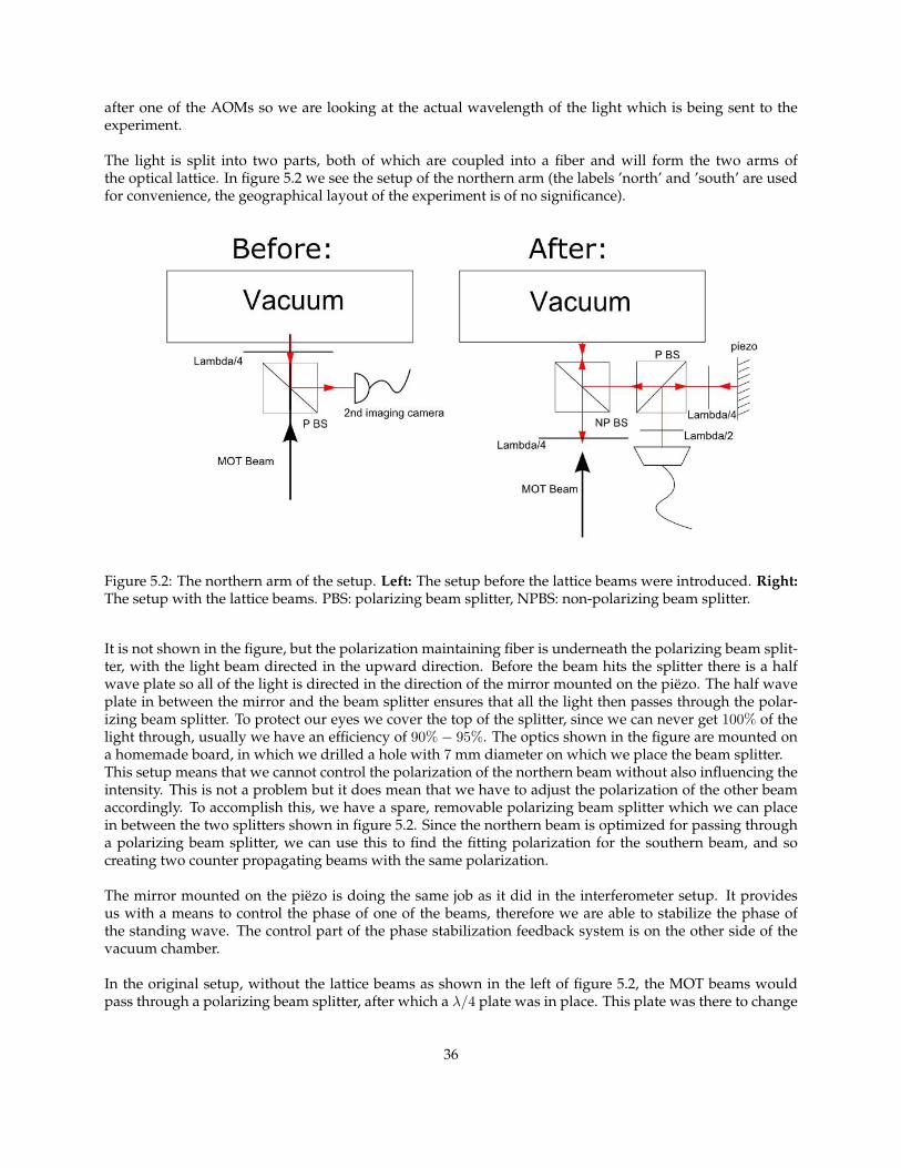
The light is split into two parts, both of which are coupled into a fiber and will form the two arms ofthe optical lattice. In figure 5.2 we see the setup of the northern arm (the labels ’north’ and ’south’ are usedfor convenience, the geographical layout of the experiment is of no significance).

Figure 5.2: The northern arm of the setup. Left: The setup before the lattice beams were introduced. Right:The setup with the lattice beams. PBS: polarizing beam splitter, NPBS: non-polarizing beam splitter.

It is not shown in the figure, but the polarization maintaining fiber is underneath the polarizing beam split-ter, with the light beam directed in the upward direction. Before the beam hits the splitter there is a halfwave plate so all of the light is directed in the direction of the mirror mounted on the piezo. The half waveplate in between the mirror and the beam splitter ensures that all the light then passes through the polar-izing beam splitter. To protect our eyes we cover the top of the splitter, since we can never get 100% of thelight through, usually we have an efficiency of 90% − 95%. The optics shown in the figure are mounted ona homemade board, in which we drilled a hole with 7 mm diameter on which we place the beam splitter.This setup means that we cannot control the polarization of the northern beam without also influencing theintensity. This is not a problem but it does mean that we have to adjust the polarization of the other beamaccordingly. To accomplish this, we have a spare, removable polarizing beam splitter which we can placein between the two splitters shown in figure 5.2. Since the northern beam is optimized for passing througha polarizing beam splitter, we can use this to find the fitting polarization for the southern beam, and socreating two counter propagating beams with the same polarization.

The mirror mounted on the piezo is doing the same job as it did in the interferometer setup. It providesus with a means to control the phase of one of the beams, therefore we are able to stabilize the phase ofthe standing wave. The control part of the phase stabilization feedback system is on the other side of thevacuum chamber.

In the original setup, without the lattice beams as shown in the left of figure 5.2, the MOT beams wouldpass through a polarizing beam splitter, after which a λ/4 plate was in place. This plate was there to change

36

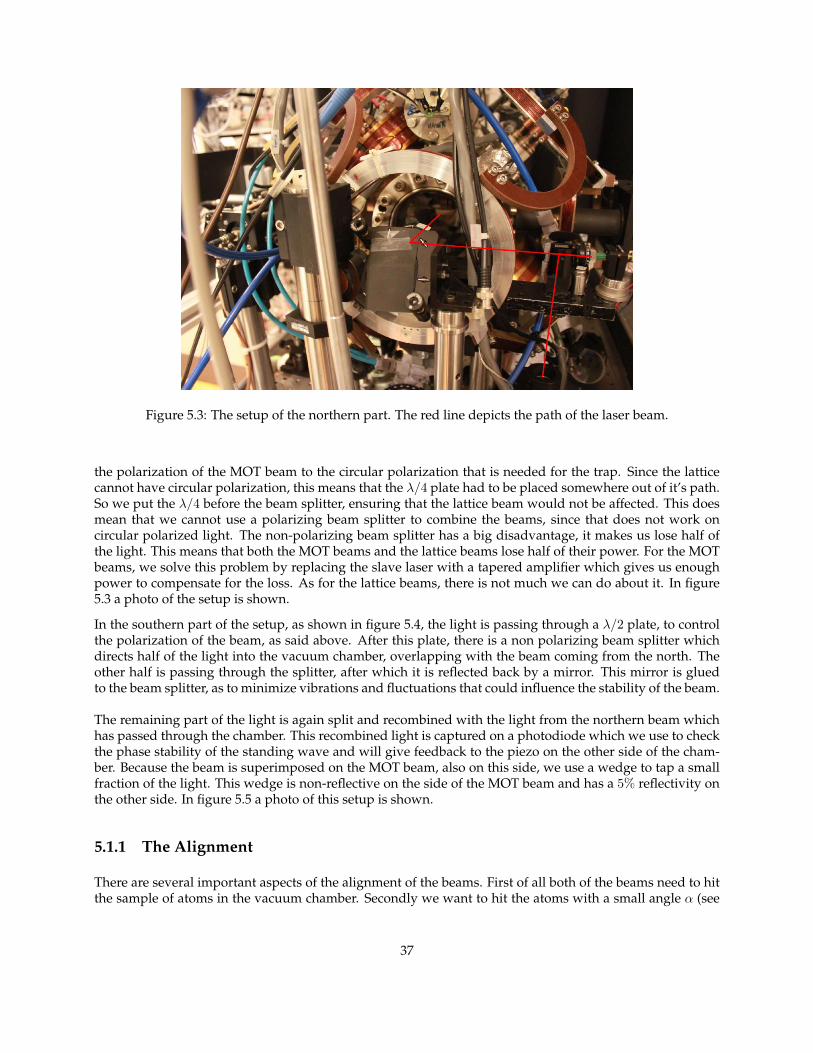
Figure 5.3: The setup of the northern part. The red line depicts the path of the laser beam.

the polarization of the MOT beam to the circular polarization that is needed for the trap. Since the latticecannot have circular polarization, this means that the λ/4 plate had to be placed somewhere out of it’s path.So we put the λ/4 before the beam splitter, ensuring that the lattice beam would not be affected. This doesmean that we cannot use a polarizing beam splitter to combine the beams, since that does not work oncircular polarized light. The non-polarizing beam splitter has a big disadvantage, it makes us lose half ofthe light. This means that both the MOT beams and the lattice beams lose half of their power. For the MOTbeams, we solve this problem by replacing the slave laser with a tapered amplifier which gives us enoughpower to compensate for the loss. As for the lattice beams, there is not much we can do about it. In figure5.3 a photo of the setup is shown.

In the southern part of the setup, as shown in figure 5.4, the light is passing through a λ/2 plate, to controlthe polarization of the beam, as said above. After this plate, there is a non polarizing beam splitter whichdirects half of the light into the vacuum chamber, overlapping with the beam coming from the north. Theother half is passing through the splitter, after which it is reflected back by a mirror. This mirror is gluedto the beam splitter, as to minimize vibrations and fluctuations that could influence the stability of the beam.

The remaining part of the light is again split and recombined with the light from the northern beam whichhas passed through the chamber. This recombined light is captured on a photodiode which we use to checkthe phase stability of the standing wave and will give feedback to the piezo on the other side of the cham-ber. Because the beam is superimposed on the MOT beam, also on this side, we use a wedge to tap a smallfraction of the light. This wedge is non-reflective on the side of the MOT beam and has a 5% reflectivity onthe other side. In figure 5.5 a photo of this setup is shown.

5.1.1 The Alignment

There are several important aspects of the alignment of the beams. First of all both of the beams need to hitthe sample of atoms in the vacuum chamber. Secondly we want to hit the atoms with a small angle α (see

37

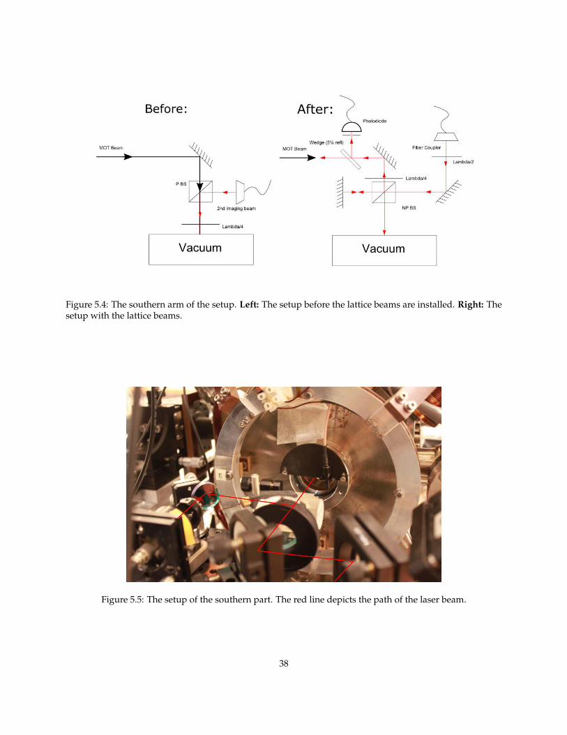
Figure 5.4: The southern arm of the setup. Left: The setup before the lattice beams are installed. Right: Thesetup with the lattice beams.

Figure 5.5: The setup of the southern part. The red line depicts the path of the laser beam.

38

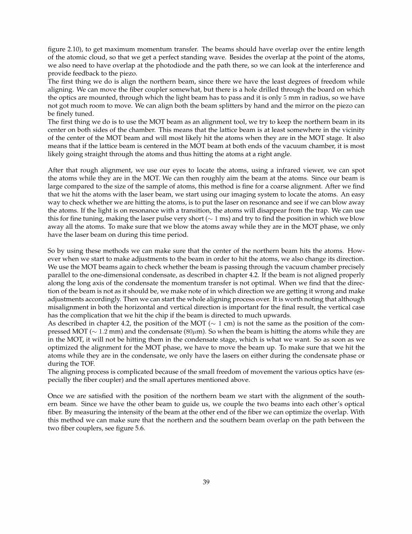
figure 2.10), to get maximum momentum transfer. The beams should have overlap over the entire lengthof the atomic cloud, so that we get a perfect standing wave. Besides the overlap at the point of the atoms,we also need to have overlap at the photodiode and the path there, so we can look at the interference andprovide feedback to the piezo.The first thing we do is align the northern beam, since there we have the least degrees of freedom whilealigning. We can move the fiber coupler somewhat, but there is a hole drilled through the board on whichthe optics are mounted, through which the light beam has to pass and it is only 5 mm in radius, so we havenot got much room to move. We can align both the beam splitters by hand and the mirror on the piezo canbe finely tuned.The first thing we do is to use the MOT beam as an alignment tool, we try to keep the northern beam in itscenter on both sides of the chamber. This means that the lattice beam is at least somewhere in the vicinityof the center of the MOT beam and will most likely hit the atoms when they are in the MOT stage. It alsomeans that if the lattice beam is centered in the MOT beam at both ends of the vacuum chamber, it is mostlikely going straight through the atoms and thus hitting the atoms at a right angle.

After that rough alignment, we use our eyes to locate the atoms, using a infrared viewer, we can spotthe atoms while they are in the MOT. We can then roughly aim the beam at the atoms. Since our beam islarge compared to the size of the sample of atoms, this method is fine for a coarse alignment. After we findthat we hit the atoms with the laser beam, we start using our imaging system to locate the atoms. An easyway to check whether we are hitting the atoms, is to put the laser on resonance and see if we can blow awaythe atoms. If the light is on resonance with a transition, the atoms will disappear from the trap. We can usethis for fine tuning, making the laser pulse very short (∼ 1 ms) and try to find the position in which we blowaway all the atoms. To make sure that we blow the atoms away while they are in the MOT phase, we onlyhave the laser beam on during this time period.

So by using these methods we can make sure that the center of the northern beam hits the atoms. How-ever when we start to make adjustments to the beam in order to hit the atoms, we also change its direction.We use the MOT beams again to check whether the beam is passing through the vacuum chamber preciselyparallel to the one-dimensional condensate, as described in chapter 4.2. If the beam is not aligned properlyalong the long axis of the condensate the momentum transfer is not optimal. When we find that the direc-tion of the beam is not as it should be, we make note of in which direction we are getting it wrong and makeadjustments accordingly. Then we can start the whole aligning process over. It is worth noting that althoughmisalignment in both the horizontal and vertical direction is important for the final result, the vertical casehas the complication that we hit the chip if the beam is directed to much upwards.As described in chapter 4.2, the position of the MOT (∼ 1 cm) is not the same as the position of the com-pressed MOT (∼ 1.2 mm) and the condensate (80µm). So when the beam is hitting the atoms while they arein the MOT, it will not be hitting them in the condensate stage, which is what we want. So as soon as weoptimized the alignment for the MOT phase, we have to move the beam up. To make sure that we hit theatoms while they are in the condensate, we only have the lasers on either during the condensate phase orduring the TOF.The aligning process is complicated because of the small freedom of movement the various optics have (es-pecially the fiber coupler) and the small apertures mentioned above.

Once we are satisfied with the position of the northern beam we start with the alignment of the south-ern beam. Since we have the other beam to guide us, we couple the two beams into each other’s opticalfiber. By measuring the intensity of the beam at the other end of the fiber we can optimize the overlap. Withthis method we can make sure that the northern and the southern beam overlap on the path between thetwo fiber couplers, see figure 5.6.

39

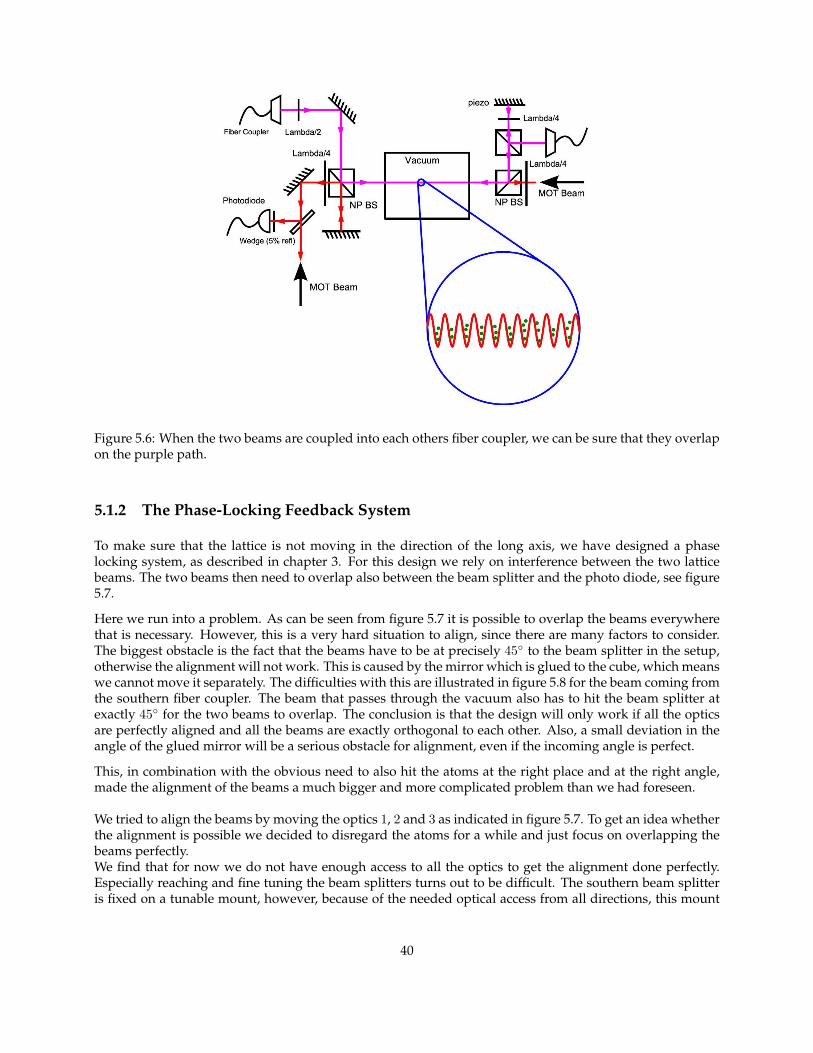
Figure 5.6: When the two beams are coupled into each others fiber coupler, we can be sure that they overlapon the purple path.

5.1.2 The Phase-Locking Feedback System

To make sure that the lattice is not moving in the direction of the long axis, we have designed a phaselocking system, as described in chapter 3. For this design we rely on interference between the two latticebeams. The two beams then need to overlap also between the beam splitter and the photo diode, see figure5.7.

Here we run into a problem. As can be seen from figure 5.7 it is possible to overlap the beams everywherethat is necessary. However, this is a very hard situation to align, since there are many factors to consider.The biggest obstacle is the fact that the beams have to be at precisely 45 to the beam splitter in the setup,otherwise the alignment will not work. This is caused by the mirror which is glued to the cube, which meanswe cannot move it separately. The difficulties with this are illustrated in figure 5.8 for the beam coming fromthe southern fiber coupler. The beam that passes through the vacuum also has to hit the beam splitter atexactly 45 for the two beams to overlap. The conclusion is that the design will only work if all the opticsare perfectly aligned and all the beams are exactly orthogonal to each other. Also, a small deviation in theangle of the glued mirror will be a serious obstacle for alignment, even if the incoming angle is perfect.

This, in combination with the obvious need to also hit the atoms at the right place and at the right angle,made the alignment of the beams a much bigger and more complicated problem than we had foreseen.

We tried to align the beams by moving the optics 1, 2 and 3 as indicated in figure 5.7. To get an idea whetherthe alignment is possible we decided to disregard the atoms for a while and just focus on overlapping thebeams perfectly.We find that for now we do not have enough access to all the optics to get the alignment done perfectly.Especially reaching and fine tuning the beam splitters turns out to be difficult. The southern beam splitteris fixed on a tunable mount, however, because of the needed optical access from all directions, this mount

40

Figure 5.7: For the phase locking system, the beams have to overlap on the purple path.

Figure 5.8: If the incoming beam is not at precisely 45 with respect to the cube, the alignment is impossible.

only works in the horizontal plane. Adjustments in other directions have to be done by hand. This proves tobe practically impossible to get right. The northern splitter is not mounted on anything but the board and iseven harder to reach than the other one. Since we do not have unlimited time we have decided at this pointto leave the phase locking system alone for now and focus on the optical lattice and the atoms. As seen in

41

Figure 5.9: The used time frame. There are two variables that we can vary, tdelay and τLatt. The startingpoint is when we release the atoms from the trap and the expansion begins. The maximum time of flight is14 ms, it is limited by the atoms falling out of view of the imaging camera.

chapter 3 the lattice is reasonably stable without the locking, especially for short time scales, which is whatwe plan to use for now.

5.2 Applying the optical lattice

Now we have aligned the beams so that they hit the atoms it is time to look at the effect of the light on thesample. We want to hit the atoms while they are in the condensate phase therefore we use the time framethat is shown in figure 5.9. We can vary the time we let the atoms expand before we turn on the latticebeams, this time we call tdelay , also we can control the time the lattice beams are on, this time is called τLatt.

The first thing we look at, an easy thing to check, is the size of the beams. If we keep the frequency of thebeams on resonance so that the atoms will be blown away, we can see how long the atoms are in the beamduring their time of flight. In 14 ms the atoms fall ∼ 1 mm. We expect the beam waist of the lattice beamsto be much larger than this, but we have to check.

We use the spectroscopy unit to determine how far detuned we are from the transition. However, it turnsout the laser diode we are using is not very single-mode in frequency. This gives us some problems lockingthe laser to the transition, because the signal is too weak. We have a contrast of about 10%, notwithstandingnumerous efforts to make it better. So to make sure that we blow the atoms away we keep on scanning overa frequency range which includes the transition frequency of the D2 at 780.24 nm [39]. We keep the beamson for 0.5 ms, as to make sure that we hit the transition at some point. In figure 5.10 the result is shown.We see that the atoms get blown away by the lattice beams all the time. In this measurement we only lookat a time of flight of 10 ms. There are some points where we do see atoms, we contribute this to the scan notreaching the transition frequency, since the scan time is slightly longer than the time the beams are on. Wecan conclude that the beam waist is large enough for the light to hit the atoms at all times.

Of course we want to make sure that it is the lattice beams that are blowing the atoms away and not another,sofar unknown, factor, we do the same experiment only with the laser far off resonance. This means thatthe atoms will not be blown away. The result is shown in figure 5.11.We can conclude that there are atoms when we detune the laser far from the resonance. Thus, the blowingaway in figure 5.10 is due to the lattice beams.

So far all we have observed is the atoms being blown away completely. The next thing we try is to see whathappens when we put the laser close to resonance so we can observe other effects of the lattice.

As we have seen in chapter 2, we can expect to see a few different situations, depending on the time thelattice beams are on and the intensity of the lattice. First we want to know how deep our lattice is. To cal-culate this we need to know several parameters. First we need to know the beam diameter and its intensity.The power in both beams is estimated to be ∼ 2 mW and the beam diameter is ∼ 3 mm. For the saturation

42

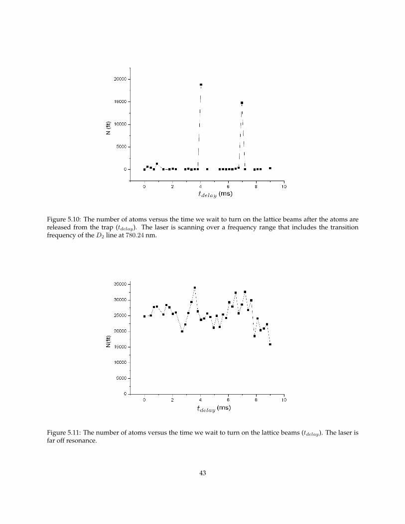
Figure 5.10: The number of atoms versus the time we wait to turn on the lattice beams after the atoms arereleased from the trap (tdelay). The laser is scanning over a frequency range that includes the transitionfrequency of the D2 line at 780.24 nm.

Figure 5.11: The number of atoms versus the time we wait to turn on the lattice beams (tdelay). The laser isfar off resonance.

43

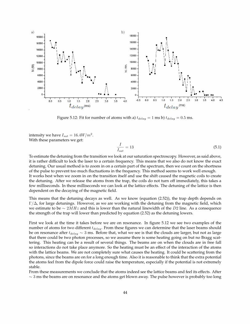
Figure 5.12: Fit for number of atoms with a) tdelay = 1 ms b) tdelay = 0.5 ms.

intensity we have Isat = 16.4W/m2.With these parameters we get:

I

Isat= 13 (5.1)

To estimate the detuning from the transition we look at our saturation spectroscopy. However, as said above,it is rather difficult to lock the laser to a certain frequency. This means that we also do not know the exactdetuning. Our usual method is to zoom in on a certain part of the spectrum, then we count on the shortnessof the pulse to prevent too much fluctuations in the frequency. This method seems to work well enough.It works best when we zoom in on the transition itself and use the shift caused the magnetic coils to createthe detuning. After we release the atoms from the trap, the coils do not turn off immediately, this takes afew milliseconds. In these milliseconds we can look at the lattice effects. The detuning of the lattice is thendependent on the decaying of the magnetic field.

This means that the detuning decays as well. As we know (equation (2.52)), the trap depth depends onΓ/∆, for large detunings. However, as we are working with the detuning from the magnetic field, whichwe estimate to be ∼ 2MHz and this is lower than the natural linewidth of the D2 line. As a consequencethe strength of the trap will lower than predicted by equation (2.52) as the detuning lowers.

First we look at the time it takes before we are on resonance. In figure 5.12 we see two examples of thenumber of atoms for two different tdelay . From these figures we can determine that the laser beams shouldbe on resonance after tdelay ∼ 3 ms. Before that, what we see is that the clouds are larger, but not as largethat there could be two photon processes, so we assume there is some heating going on but no Bragg scat-tering. This heating can be a result of several things. The beams are on when the clouds are in free fallso interactions do not take place anymore. So the heating must be an effect of the interaction of the atomswith the lattice beams. We are not completely sure what causes the heating. It could be scattering from thephotons, since the beams are on for a long enough time. Also it is reasonable to think that the extra potentialthe atoms feel from the dipole force could raise the temperature, especially if the potential is not extremelystable.From these measurements we conclude that the atoms indeed see the lattice beams and feel its effects. After∼ 3 ms the beams are on resonance and the atoms get blown away. The pulse however is probably too long

44

for Bragg scattering, so we try to shorten the pulse.

When we greatly shorten the pulse duration we start to see other effects. With these short times shouldsee Bragg diffraction, as described in chapter 2.3.2. We expect to perform a two-photon process, which willresult in the transfer of momentum from the photons to the atoms. Since the atoms can only absorb q = 0k,q = 2k, q = 4k etcetera, we expect to see well-defined Bragg peaks. To perform Bragg spectroscopy, we needto vary the frequency difference between the two beams.

45

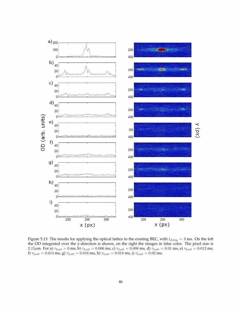
Figure 5.13: The results for applying the optical lattice to the existing BEC, with tdelay = 3 ms. On the leftthe OD integrated over the y-direction is shown, on the right the images in false color. The pixel size is2.15µm. For a) τLatt = 0 ms, b) τLatt = 0.006 ms, c) τLatt = 0.008 ms, d) τLatt = 0.01 ms, e) τLatt = 0.012 ms,f) τLatt = 0.014 ms, g) τLatt = 0.016 ms, h) τLatt = 0.018 ms, i) τLatt = 0.02 ms.

46

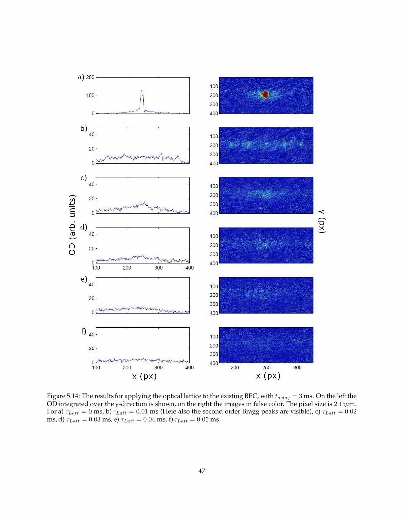
Figure 5.14: The results for applying the optical lattice to the existing BEC, with tdelay = 3 ms. On the left theOD integrated over the y-direction is shown, on the right the images in false color. The pixel size is 2.15µm.For a) τLatt = 0 ms, b) τLatt = 0.01 ms (Here also the second order Bragg peaks are visible), c) τLatt = 0.02ms, d) τLatt = 0.03 ms, e) τLatt = 0.04 ms, f) τLatt = 0.05 ms.

47

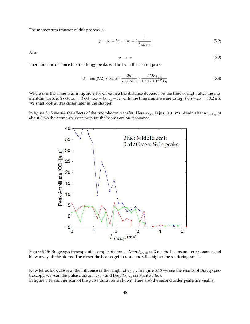
The momentum transfer of this process is:

p = p0 + ~q0 = p0 + 2h

λphoton(5.2)

Also:p = mv (5.3)

Therefore, the distance the first Bragg peaks will be from the central peak:

d = sin(θ/2) ∗ cosα ∗ 2h780.2nm

∗ TOFLatt

1.44 ∗ 10−25kg(5.4)

Where α is the same α as in figure 2.10. Of course the distance depends on the time of flight after the mo-mentum transfer TOFLatt = TOFTotal − tdelay − τLatt. In the time frame we are using, TOFTotal = 13.2 ms.We shall look at this closer later in the chapter.

In figure 5.15 we see the effects of the two photon transfer. Here τLatt is just 0.01 ms. Again after a tdelay ofabout 3 ms the atoms are gone because the beams are on resonance.

Figure 5.15: Bragg spectroscopy of a sample of atoms. After tdelay ≈ 3 ms the beams are on resonance andblow away all the atoms. The closer the beams get to resonance, the higher the scattering rate is.

Now let us look closer at the influence of the length of τLatt. In figure 5.13 we see the results of Bragg spec-troscopy, we scan the pulse duration τLatt and keep tdelay constant at 3ms.In figure 5.14 another scan of the pulse duration is shown. Here also the second order peaks are visible.

48

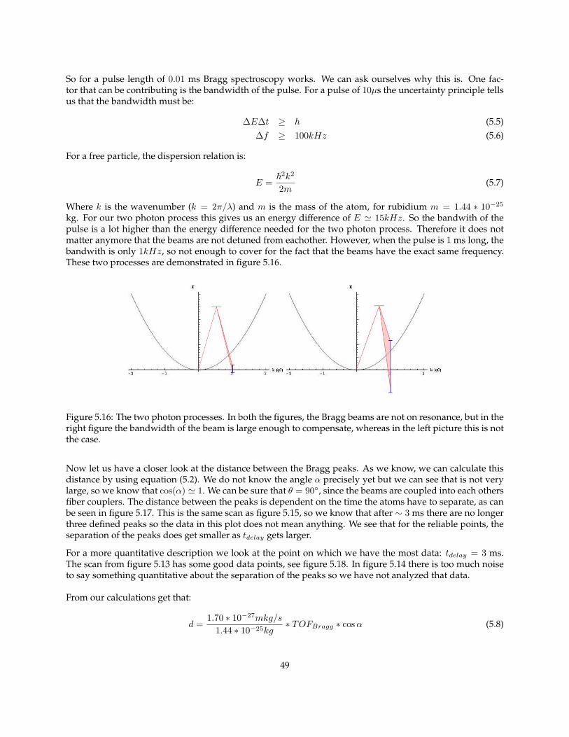
So for a pulse length of 0.01 ms Bragg spectroscopy works. We can ask ourselves why this is. One fac-tor that can be contributing is the bandwidth of the pulse. For a pulse of 10µs the uncertainty principle tellsus that the bandwidth must be:

∆E∆t ≥ h (5.5)∆f ≥ 100kHz (5.6)

For a free particle, the dispersion relation is:

E =~2k2

2m(5.7)

Where k is the wavenumber (k = 2π/λ) and m is the mass of the atom, for rubidium m = 1.44 ∗ 10−25

kg. For our two photon process this gives us an energy difference of E ' 15kHz. So the bandwith of thepulse is a lot higher than the energy difference needed for the two photon process. Therefore it does notmatter anymore that the beams are not detuned from eachother. However, when the pulse is 1 ms long, thebandwith is only 1kHz, so not enough to cover for the fact that the beams have the exact same frequency.These two processes are demonstrated in figure 5.16.

Figure 5.16: The two photon processes. In both the figures, the Bragg beams are not on resonance, but in theright figure the bandwidth of the beam is large enough to compensate, whereas in the left picture this is notthe case.

Now let us have a closer look at the distance between the Bragg peaks. As we know, we can calculate thisdistance by using equation (5.2). We do not know the angle α precisely yet but we can see that is not verylarge, so we know that cos(α) ' 1. We can be sure that θ = 90, since the beams are coupled into each othersfiber couplers. The distance between the peaks is dependent on the time the atoms have to separate, as canbe seen in figure 5.17. This is the same scan as figure 5.15, so we know that after ∼ 3 ms there are no longerthree defined peaks so the data in this plot does not mean anything. We see that for the reliable points, theseparation of the peaks does get smaller as tdelay gets larger.

For a more quantitative description we look at the point on which we have the most data: tdelay = 3 ms.The scan from figure 5.13 has some good data points, see figure 5.18. In figure 5.14 there is too much noiseto say something quantitative about the separation of the peaks so we have not analyzed that data.

From our calculations get that:

d =1.70 ∗ 10−27mkg/s

1.44 ∗ 10−25kg∗ TOFBragg ∗ cosα (5.8)

49

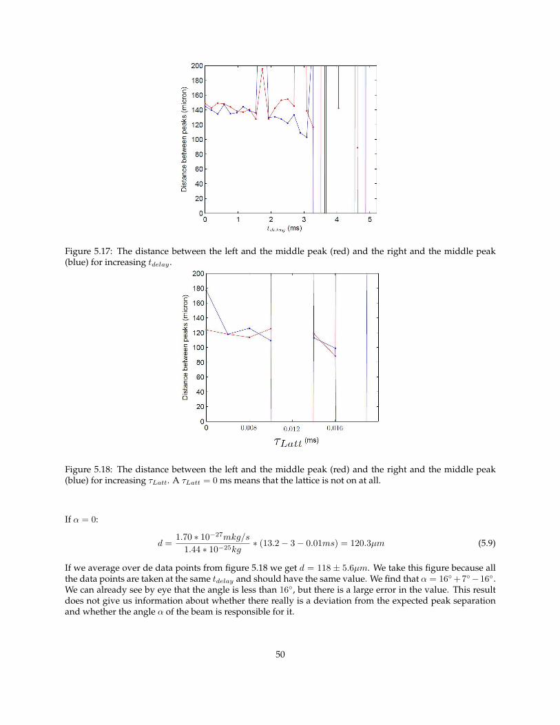
Figure 5.17: The distance between the left and the middle peak (red) and the right and the middle peak(blue) for increasing tdelay .

Figure 5.18: The distance between the left and the middle peak (red) and the right and the middle peak(blue) for increasing τLatt. A τLatt = 0 ms means that the lattice is not on at all.

If α = 0:

d =1.70 ∗ 10−27mkg/s

1.44 ∗ 10−25kg∗ (13.2− 3− 0.01ms) = 120.3µm (5.9)

If we average over de data points from figure 5.18 we get d = 118 ± 5.6µm. We take this figure because allthe data points are taken at the same tdelay and should have the same value. We find that α = 16+7−16.We can already see by eye that the angle is less than 16, but there is a large error in the value. This resultdoes not give us information about whether there really is a deviation from the expected peak separationand whether the angle α of the beam is responsible for it.

50

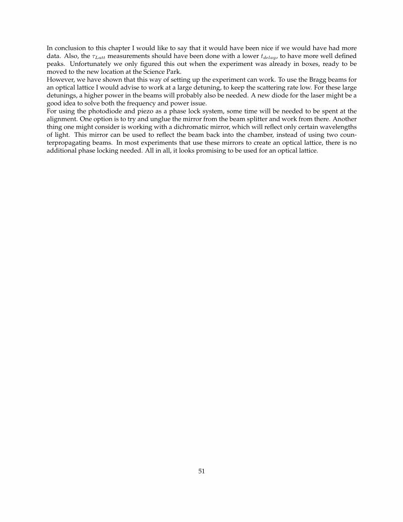
In conclusion to this chapter I would like to say that it would have been nice if we would have had moredata. Also, the τLatt measurements should have been done with a lower tdelay , to have more well definedpeaks. Unfortunately we only figured this out when the experiment was already in boxes, ready to bemoved to the new location at the Science Park.However, we have shown that this way of setting up the experiment can work. To use the Bragg beams foran optical lattice I would advise to work at a large detuning, to keep the scattering rate low. For these largedetunings, a higher power in the beams will probably also be needed. A new diode for the laser might be agood idea to solve both the frequency and power issue.For using the photodiode and piezo as a phase lock system, some time will be needed to be spent at thealignment. One option is to try and unglue the mirror from the beam splitter and work from there. Anotherthing one might consider is working with a dichromatic mirror, which will reflect only certain wavelengthsof light. This mirror can be used to reflect the beam back into the chamber, instead of using two coun-terpropagating beams. In most experiments that use these mirrors to create an optical lattice, there is noadditional phase locking needed. All in all, it looks promising to be used for an optical lattice.

51

Chapter 6

Conclusion and Outlook

So after all is said and done and this thesis is almost finished, I am left with the task to reflect on the work Ihave done, to identify corrections that can be made and to tell you what I think could happen in the futureof this experiment.

As I have said, optical lattices are widely used today in the field of cold atoms to study a variety of phe-nomena, from condensed matter simulation to Anderson localization to quantum computing. With opticallattices, one can access a two-dimensional or even one-dimensional regime. For a array of two dimensionalpancakes, one would need a three dimensional cloud of cold atoms and two orthogonal beams to create aperiodic confinement. To create an array of one-dimensional tubes, only one more pair of beams is needed.Another pair of beams will than create a cubic array of tightly confining harmonic oscillator potentials ateach lattice site.We differ from most one-dimensional lattice experiments, for the reason that we are working with coldatoms that are already in a one-dimensional confinement. By adding optical lattice beams we will create anstring of lattice sites. The big difference is that when we measure, we do not have to average over more thanone site, which means that we can focus on small fluctuations that otherwise would get lost in the biggernumbers.

The task of this project was designing, testing and building the system that would provide the lattice beams.In this thesis I have reported on my progress in those areas. I think that I can say that the project was a suc-cess, we have shown that the two beams can be phase locked and will be stable enough to be used for anoptical lattice. Unfortunately the phase locking for the setup on the Celsius experiment has not worked outyet, but this is only a matter of time and effort. The easiest solution for this problem will be to separate thebeam splitter and the mirror. This will give us extra freedom and make it easy to align the phase stabiliza-tion part of the setup.Another possibility we could look at, is to switch from two separate beams to one beam that is retro reflectedby a dichromatic mirror. This mirror would then let the MOT beam pass through and will only reflect thelattice beam. An advantage of a setup like this is that you do not need additional phase stabilizing, as longas the mirror is stable. Also the power in the beam is twice that of two separate beams. To make up for theabsorption in the first passage through the atoms, we can slightly curve the mirror to focus the beam. Adownside is that you lose control over the relative frequency of the two beams, so Bragg spectroscopy is nolonger possible. One can also argue that an active phase feedback system provides a better stability than amirror, since you are actively compensating for the instability in all the optics that are involved.For now we only have been using the beams for scattering atoms of the optical grating we created, if wewant to create a lattice in which we can load the atoms for a longer time, some other things will probablyneed to change. For one thing, right now we are working with light that is very near the resonance and as

52

a result we have very high scattering rates. This will not work if the atoms have to stay in the lattice forlonger times. Therefore I would suggest that we take a laser that is slightly further off resonance than theone we are using now. For the exact wavelength of the light, I would say that it is not extremely importantas long as it is > 15 nm away from the transition, as to keep the scattering rate low enough. It is probablyeasiest to look for a convenient laser that will provide such light. Also, for such a large detuning, we willneed a bit more power to get large lattices that can create Mott insulators.With those minor adjustments out of the way, I must say that I think that the setup for the lattice can workvery well. It should be very interesting to make a string of small ensembles of atoms and study the quantumfluctuations.

I have greatly enjoyed learning how to work in an optics lab and creating the report that you are read-ing today. I would like to thank all the people at the Celsius experiment very much for all their advise,support and help, I could not have done it without you.

53

Chapter 7

Populaire Samenvatting

Voor mijn Master project aan de Universiteit van Amsterdam heb ik gewerkt met ultra koude atomen. Detemperatuur van deze atomen (Rubidium 87) is enkele tientallen nanoKelvin. Om atomen zo koud te krijgengebruiken we lasers. De lasers koelen de atomen en houden, in samenwerking met magneten, ze daarnaastook nog eens vast in een zogeheten magneto-optische val. We werken in een vacuum kamer, zodat we geenlast hebben van een achtergrond gas (de lucht om ons heen) dat onze Rubidium atomen opwarmt en uit deval stoot. Ons experiment creeert uiteindelijk een heel dunne sigaarvormige val, waarin de atomen maarin een richting kunnen bewegen. Ze zijn dus in de praktijk eendimensionaal. Dit krijgen we voor elkaarmet een atoom chip, een kleine chip waarom draden zitten die onder andere een magnetische val kunnenmaken. Ons experiment is anders dan andere omdat wij slechts een sigaar van atomen hebben, terwijl jevaak ziet dat experimenten bestaan uit een rij sigaren. Als je dan een meting doet, neem je het gemiddeldeover al deze sigaren. Je krijgt dan een groter signaal maar je middelt kleine effecten uit.

Ik heb een optisch rooster gebouwd voor op dit experiment. Een optisch rooster is een staande golf van licht.Als atomen erg koud zijn, kunnen ze gevangen worden door licht. Afhankelijk van de golflengte van hetlicht worden atomen aangetrokken of afgestoten door regionen met een hoge lichtintensiteit. Twee stralenvan laserlicht, overlappend in tegenovergestelde richting vormen de staande golf die we nodig hebben. Eenstaande golf van licht is een afwisseling van plekken met een hoge intensiteit (waar de twee laserstralen con-structief interfereren) en plekken met een lage intensiteit (waar de laserstralen destructief interfereren). Voorde atomen is dit dan een periodiek rooster.Deeltjes in roosters kennen we natuurlijk al van gecondenseerde materie, bijvoorbeeld elektronen in eenmetaal. Het mooie van het nabootsen van zo een systeem met koude atomen, is dat je erg veel controle hebtover je experiment. De afstand tussen de roosterpunten is afhankelijk van de golflengte van je licht en jekunt de interactie van de deeltjes controleren. Dit alles is niet mogelijk met een metaal. Een van de meestbelangrijke voordelen is nog wel dat er in een optisch rooster geen imperfecties zijn die het experimentbeınvloeden. Al deze dingen bij elkaar maken koude atomen in optische roosters een erg aantrekkelijkemogelijkheid voor simulatie van gecondenseerde materie.Een optisch rooster op een eendimensie creeert een ketting van kleine wolkjes atomen. Ons doel is om indeze kleine ensembles fluctuaties the bestuderen.

Om dit alles voor elkaar te krijgen, heb ik het laser systeem waarmee ik heb gewerkt, gebouwd. Dit be-stond uit het in elkaar zetten van de laser, het bouwen van een versterker en het splitsen van de laserstraalin twee dezelfde stralen, waarvan we de intensiteit en de relatieve frequentie konden controleren. Daarnaheb ik een ontwerp gemaakt voor het uiteindelijke systeem dat we op het experiment hebben gebouwd,en door een interferometer te bouwen en daarmee de stabiliteit te testen, een aantal aanpassingen gedaan.Hierna heb ik het rooster op het echte experiment gebouwd en een aantal metingen gedaan.

54

Bibliography

[1] A. Einstein, Sitzber. Kgl. Preuss. Akad. Wiss., 261 (1924); ibidem, 3 (1925)

[2] S.N. Bose, Z. Phys. 26, 178 (1924)

[3] L. Pitaevskii and S. Stringari, Bose-Einstein Condensation, Oxford University Press (2004)

[4] M.H. Anderson, J.R. Ensher, M.R. Matthews, C.E. Wieman and E.A. Cornell, Science Vol. 269, No. 5221(1995)

[5] K. B. Davis, M. -O. Mewes, M. R. Andrews, N. J. van Druten, D. S. Durfee, D. M. Kurn, and W. Ketterle,Phys. Rev. Lett. 75, 39693973 (1995)

[6] L. Fallani, Bose-Einstein Condensates in Optical Lattices, PhD Thesis, LENS

[7] D.S. Petrov, G.V. Shlyapnikov and J.T.M. Walraven, Phys. Rev. Lett. 85, 18 (2000)

[8] F. Dalfovo, S.Giorgini, L.P. Pitaevskii and S. Stringari, Rev. Mod. Phys. 71, 463512 (1999)

[9] W. Ketterle, and N. J. van Druten, Phys. Rev. A 54, 656(1996)

[10] C. Menotti and S. Stringari, Phys. Rev. A 66, 043610 (2002)

[11] , M. Girardeau, J. Math. Phys 1, 516-523 (1960)

[12] B. Paredes et al, Nature 429, 277 (2004)

[13] T. Kinoshita, T. Wenger and D. S. Weiss, Science 305, 1125 (2004)

[14] Bachelors Thesis A.L. Hoendervanger, University of Amsterdam 2007

[15] E. H. Lieb and W. Liniger, Phys. Rev. 130, 1650 (1963)

[16] F. Deuretzbacher, K. Bongs, K. Sengstock and D. Pfannkuche, cond-mat/0604673v4 (2007)

[17] T.W. Hansch and A.L. Schawlow, Optics Communications Vol 13, No. 1, January 1975

[18] The Nobel Prize in Physics 1997, http://nobelprize.org/nobel-prizes/physics/laureates/199

[19] E.L. Raab, M. Prentiss, A. Cable, S. Chu and D.E. Pritchard, Phys. Rev. Lett. 59, 2631 (1987)

[20] A.L. Migdall, J.V. Prodan, W.D. Philips, T.H. Bergeman and H.J. Metcalf, Phys. Rev. Lett. 54, 2596 (1985)

[21] W.H. Wing, Progr. in Quant. Elec. 8, 181 (1994)

[22] E. Majorana, Il Nuovo Cimento 9, 43 (1932)

[23] D.E. Pritchard, Phys. Rev. Lett. 51, 1336 (1983)

55

[24] R. Grimm, M. Weidemuller and Y.B. Ovchinnikov, Adv. At. Mol. Opt. Phys. 42, 95 (2000)

[25] F. Bloch, Zeitschrift Fur Physik A Volume 52, N. 7-8, 555-600 (1929)

[26] G. H. Wannier, Phys. Rev. 52, 191 (1937)

[27] M. Greiner, O. Mandel, T. Esslinger, T.W. Hansch and I. Bloch, Nature 415, 39-44 (3 January 2002)

[28] D. Clement, N. Fabbri, L. Fallani, C. Fort, and M. Inguscio, Phys. Rev. Lett. 102, 155301 (2009)

[29] I. Bloch, Nature Physics 1, 23 - 30 (2005)

[30] T. Stoferle, H. Moritx, C. Schori, M. Kol and T. Esslinger, Phys. Rev. Lett. 92, 130403 (2004)

[31] D. Clement, N. Fabbri, L. Fallani, C. Fort and M. Ignuscio, New Journal of Physics 11 (2009)

[32] A.A. Michelson and E. Morley, American Journal of Science 34 (203) 333345, 1887

[33] D.W. Keith, C.R. Ekstrom, Q.A. Turchette and D.E. Pritchard, Phys. Rev. Lett. 66, 2693-2696 (1991)

[34] A. van Amerongen, One-dimensional Bose gas on an atom chip, PhD Thesis, University of Amsterdam2008

[35] J. Reichel, Appl. Phys. B 75, 469-487 (2002)

[36] J. J. P. van Es, Bose-Einstein condensates in radio-frequency-dressed potentials on an atom chip, PhD Thesis,University of Amsterdam 2009

[37] J. Reichel, W. Hansel and T. W. Hansch, Phys. Rev. Lett. 83, 33983401 (1999).

[38] A.D. Cronin, J. Schiedmayer and D.E. Pritchard, Rev. of Mod. Phys 81, 2009

[39] http://steck.us/alkalidata/rubidium87numbers.1.6.pdf

56