introducing effects in an image: a matlab approach · pdf fileintroducing effects in an image:...
TRANSCRIPT

HAL Id: inria-00321624https://hal.inria.fr/inria-00321624
Submitted on 15 Sep 2008
HAL is a multi-disciplinary open accessarchive for the deposit and dissemination of sci-entific research documents, whether they are pub-lished or not. The documents may come fromteaching and research institutions in France orabroad, or from public or private research centers.
L’archive ouverte pluridisciplinaire HAL, estdestinée au dépôt et à la diffusion de documentsscientifiques de niveau recherche, publiés ou non,émanant des établissements d’enseignement et derecherche français ou étrangers, des laboratoirespublics ou privés.
Introducing Effects in an Image: A MATLAB ApproachVinay Kumar, Saurabh Sood, Shruti Mishra
To cite this version:Vinay Kumar, Saurabh Sood, Shruti Mishra. Introducing Effects in an Image: A MATLAB Approach.2008. <inria-00321624>

Introducing Effects in an Image: A
MATLAB Approach
by Vinay Kumar Saurabh Sood
And Shruti Mishra
Department of Electronics and Communication Engineering,
Jaypee University of Information Technology, Solan-173 215, INDIA

4
Table of Contents
List of Figures…………………………………………….. ……5
Abstract………………………………………………………….7
Introduction…………………………………………………….8
1. Types of Images…………………………………………...9
2. Filter Designing…………………………………………..12
3. Difference between day and night images………….......14
4. Random Experiments on image.......................................17
5. Factors Influencing an image…………………………...21
6. Effects of Night on an Image………………………........32
7. Dawn and Evening effects................................................36
Conclusion………………………………………………….....39
Bibliography………………………………………………….40

5
List of Figures
1. Chapter -1
Fig 1.1 : INTENSITY IMAGE
Fig 1.2 : BINARY IMAGE
Fig 1.3 : INDEXED IMAGE
Fig 1.4 : RGB IMAGE
2. Chapter -2
Fig 2.1: 3-D PLOT OF GAUSSIAN LOW PASS FILTER
Fig 2.2 : ORIGINAL IMAGE
Fig 2.3 : FILTERED IMAGE
3. Chapter -3
Fig 3.1: DAY IMAGE-1
Fig 3.2: NIGHT IMAGE-1
Fig 3.3: DIFFERENCE BETWEEN 4.1 AND 4.2
Fig 3.4 : DAY IMAGE -2
Fig 3.5 : AFTER SUNSET IMAGE-2
Fig 3.6 : DIFFERENCE BETWEEN 4.4 AND 4.5
4. Chapter -4
Fig 4.1: DAY IMAGE
Fig 4.2: INTENSITY HISTOGRAM OF Fig 5.1
Fig 4.3: NIGHT IMAGE
Fig 4.4: INTENSITY HISTOGRAM OF Fig 5.3
Fig 4.5: RESULT OF EDGE DETECTION ON Fig 5.1 Fig 4.6: TEXTURE ANALYSIS OF Fig 5.1

6
5. Chapter-5
Fig 5.1: HUE SCALE
Fig 5.2: YELLOW SHIFT
Fig 5.3: GREEN SHIFT
Fig 5.4: BLUE SHIFT
Fig 5.5: RED SHIFT
Fig 5.6: IMAGE WITH DIFFERENT SATURATION LEVELS
Fig 5.7: ORIGINAL DAY IMAGE
Fig 5.8: BRIGHTENESS OF Fig 5.7 DECREASED BY 20 PERCENT
Fig 5.9: BRIGHTENESS OF Fig 5.7 DECREASED BY 40 PERCENT
Fig 5.10: BRIGHTENESS OF Fig 5.7 DECREASED BY 50 PERCENT
Fig 5.11: BRIGHTENESS OF Fig 5.7 DECREASED BY 60 PERCENT
Fig 5.12: BRIGHTENESS OF Fig 5.7 DECREASED BY 70 PERCENT
Fig 5.13: BRIGHTENESS OF Fig 5.7 DECREASED BY 80 PERCENT
Fig 5.14: BRIGHTENESS OF Fig 5.7 DECREASED BY 90 PERCENT
Fig 5.15: BRIGHTENESS OF Fig 5.7 DECREASED BY 100 PERCENT
Fig 5.16: RELATIONSHIP OF PIXEL VALUES TO DISPLAY
6. Chapter -6
Fig 6.1: DAY IMAGE-1
Fig 6.2: FULL MOON LIGHT IMAGE OF Fig 6.1
Fig 6.3: DAY IMAGE -2
Fig 6.4: FULL MOON LIGHT IMAGE OF Fig 6.3
Fig 6.5: DAY IMAGE -3
Fig 6.6: FULL MOON LIGHT IMAGE OF Fig 6.5
7. Chapter -7
Fig 7.1: DAY IMAGE 1
Fig 7.2: EVENING IMAGE FOR Fig. 7.1
Fig 7.3: DAY IMAGE 2
Fig 7.4: DAWN IMAGE FOR Fig 7.3

7
Abstract
The standard technique for making images viewed at daytime lighting levels look like
images of night scenes is to use a low overall contrast, low overall brightness,
desaturation, and to give the image a “blue shift". Moonlit night scenes have a tinge of
blue. Earlier work to model this perceptual effect has been statistical in nature; often
based on unreliable measurements of blueness in paintings of moonlit night scenes.In
Digital Image Processing we implement all these factors to derive the desired results.

8
INTRODUCTION
A digital image is composed of pixels which can be thought of as small dots on the
screen. A digital image is an instruction of how to color each pixel. In the general case
we say that an image is of size m-by-n if it is composed of m pixels in the vertical
direction and n pixels in the horizontal direction. Image formats supported by Matlab are
BMP, HDF, JPEG, PCX, TIFF, XWB In this project report we present various types of
images that are being used in Digital Image Processing. Some light has been thrown on
the difference between day and night images by utilizing their intensity histograms. We
have also discussed various attributes of an image. Finally we present the details of
augmenting the day image with loss of details associated with night vision.
.

9
CHAPTER – 1
TYPES OF IMAGES
1. Intensity image (gray scale image)
This is the equivalent to a "gray scale image" and this is the image we will mostly work
with in this course. It represents an image as a matrix where every element has a value
corresponding to how bright/dark the pixel at the corresponding position should be
colored. There are two ways to represent the number that represents the brightness of
the pixel.
Fig:1.1:Intensity image

10
2. Binary image
This image format also stores an image as a matrix but can only color a pixel black or
white (and nothing in between). It assigns a 0 for black and a 1 for white.
Fig 1.2: Binary image
3. Indexed image
This is a practical way of representing color images. An indexed image stores an
image as two matrices. The first matrix has the same size as the image and one
number for each pixel. The second matrix is called the color map and its size may be
different from the image. The numbers in the first matrix is an instruction of what
number to use in the color map matrix.
Fig 1.3:Indexed image

11
4. RGB image
This is another format for color images. It represents an image with three matrices of
sizes matching the image format. Each matrix corresponds to one of the colors red,
green or blue and gives an instruction of how much of each of these colors a certain
pixel should use.
Fig 1.4: RGB image
12
CHAPTER -2
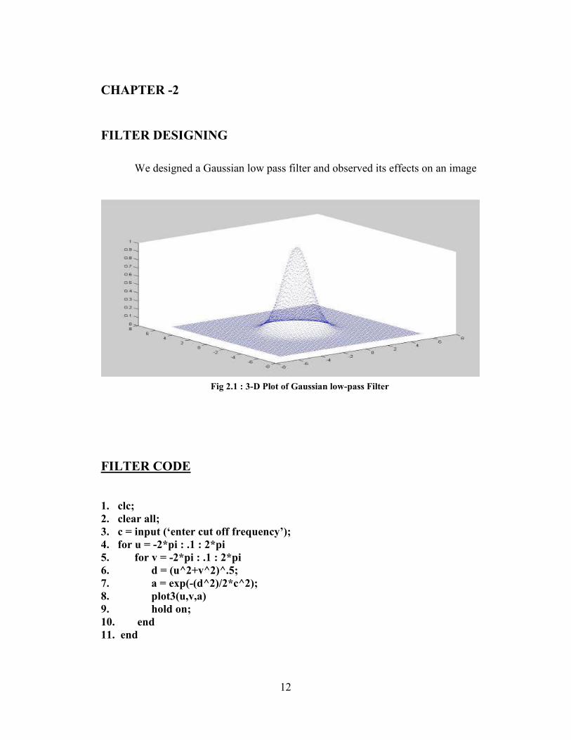
FILTER DESIGNING
We designed a Gaussian low pass filter and observed its effects on an image
FILTER CODE
1. clc;
2. clear all;
3. c = input (‘enter cut off frequency’);
4. for u = -2*pi : .1 : 2*pi
5. for v = -2*pi : .1 : 2*pi
6. d = (u^2+v^2)^.5;
7. a = exp(-(d^2)/2*c^2);
8. plot3(u,v,a)
9. hold on;
10. end
11. end
Fig 2.1 : 3-D Plot of Gaussian low-pass Filter

13
ORIGINAL IMAGE
FILTERED IMAGE
Fig 2.2
Fig 2.3

14
CHAPTER-3
DIFFERENCE BETWEEN A DAY AND A NIGHT IMAGE
Fig3.1 : Day Image
Fig3.2 : Night Image

15
ANOTHER EXAMPLE
Fig3.3 : Difference between the above images
Fig 3.4 : Day Image
16
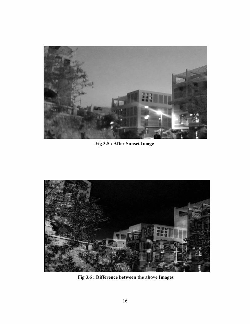
Fig 3.5 : After Sunset Image
Fig 3.6 : Difference between the above Images

17
CHAPTER - 4
RANDOM EXPERIMENTS ON AN IMAGE
1. Intensity Histogram
2. Edge detection
3. Texture
1. Intensity Histogram
We tried to find out the difference between the day and a night image
by analyzing the intensity histograms of different images.Here is one example :
Fig. 4.1: Day Image

18
Fig 4.2 : Intensity Histogram of Fig 4.1
Fig 4.3 : After Sunset Image

19
2. Edge Detection
In an image an edge is a curve that follows a path of rapid change in image
intensity.Edges are often associated with boundaries of objects. Edge function looks for
places where intensities change rapidly
Fig 4.4 : Intensity Histogram of Fig 4.3
Fig 4.5 : Result of edge detection on fig 4.1
20
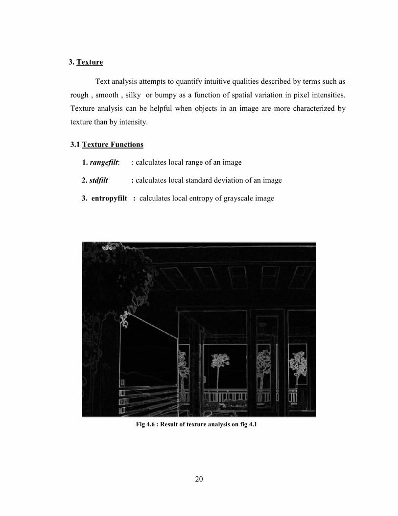
3. Texture
Text analysis attempts to quantify intuitive qualities described by terms such as
rough , smooth , silky or bumpy as a function of spatial variation in pixel intensities. Texture analysis can be helpful when objects in an image are more characterized by
texture than by intensity.
3.1 Texture Functions
1. rangefilt: : calculates local range of an image
2. stdfilt : calculates local standard deviation of an image
3. entropyfilt : calculates local entropy of grayscale image
Fig 4.6 : Result of texture analysis on fig 4.1

21
CHAPTER – 5
FACTORS INFLUENCING AN IMAGE
1. Hue
2. Saturation
3. Brightness
4. Contrast
1. HUE
Hue is one of the three main attributes of perceived color, in addition to
lightness and chroma (or colorfulness). Hue is also one of the three dimensions in
some color spaces along with saturation, and brightness (also known as lightness or
value). Hue is that aspect of a color described with names such as "red", "yellow",
etc.
Usually, colors with the same hue are distinguished with adjectives referring to their
lightness and/or chroma, such as with "light blue", "pastel blue", "vivid blue". Notable
exceptions include brown, which is a dark orange and pink, a light red with reduced
chroma.
In painting color theory, a hue refers to a pure color—one without tint or shade (added
white or black pigment, respectively).A hue is an element of the color wheel.
Fig 5.1 : Hue scale

22
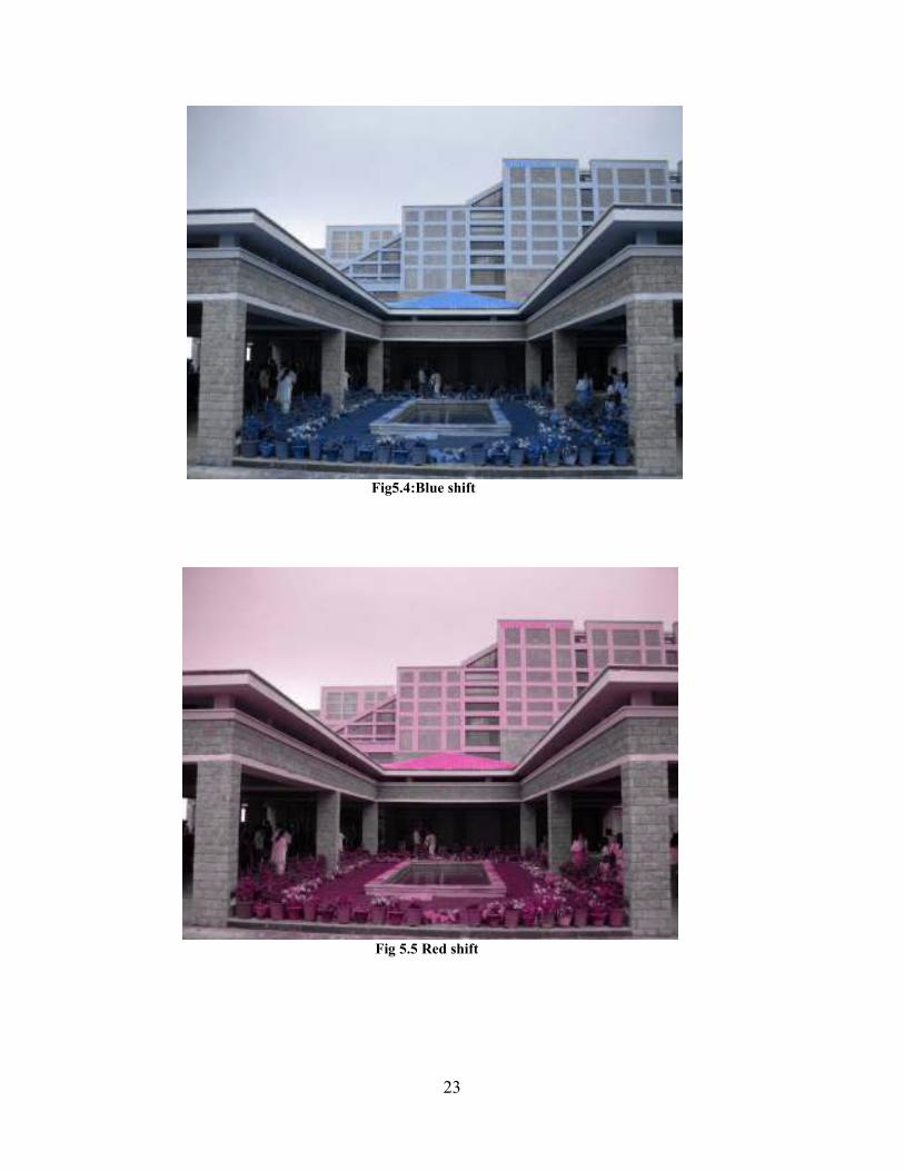
Images with different hues on hue scale
Fig 5.2: Yellow shift
Fig 5.3:Green shift
23
Fig5.4:Blue shift
Fig 5.5 Red shift
24
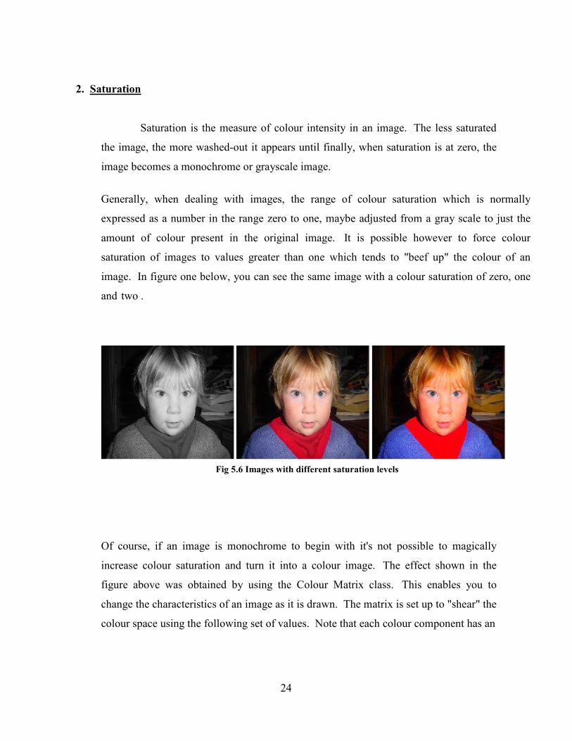
2. Saturation
Saturation is the measure of colour intensity in an image. The less saturated
the image, the more washed-out it appears until finally, when saturation is at zero, the
image becomes a monochrome or grayscale image.
Generally, when dealing with images, the range of colour saturation which is normally
expressed as a number in the range zero to one, maybe adjusted from a gray scale to just the
amount of colour present in the original image. It is possible however to force colour
saturation of images to values greater than one which tends to "beef up" the colour of an
image. In figure one below, you can see the same image with a colour saturation of zero, one
and two .
Of course, if an image is monochrome to begin with it's not possible to magically
increase colour saturation and turn it into a colour image. The effect shown in the
figure above was obtained by using the Colour Matrix class. This enables you to
change the characteristics of an image as it is drawn. The matrix is set up to "shear" the
colour space using the following set of values. Note that each colour component has an
Fig 5.6 Images with different saturation levels
25
effective luminance which contributes to the overall brightness of the pixel. The
effective luminance value for red is 0.3086. Green has an effective luminance of
0.6094 and the value for blue is 0.082. The reciprocal of the saturation value is
multiplied by the effective luminance of the colour component to produce a value by
which each colour component of each pixel is multiplied during the matrix operation
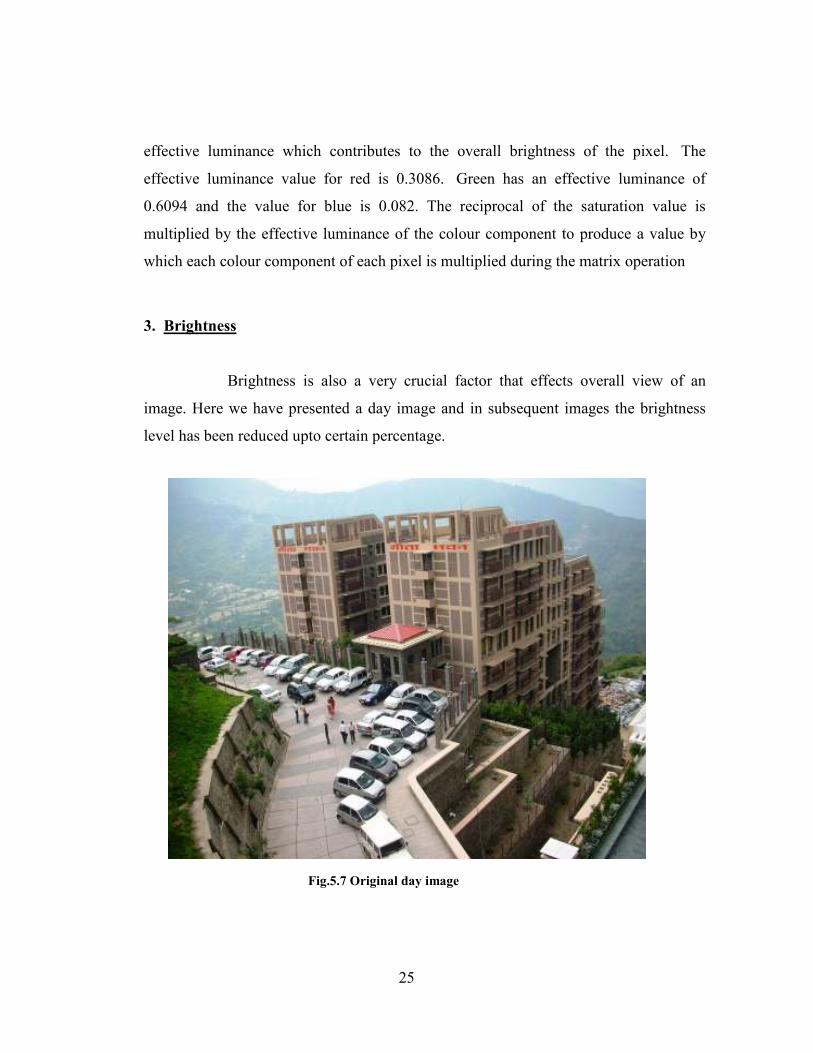
3. Brightness
Brightness is also a very crucial factor that effects overall view of an
image. Here we have presented a day image and in subsequent images the brightness
level has been reduced upto certain percentage.
Fig.5.7 Original day image

26
Fig 5.8 : Brightness decreased by 20 percent
Fig 5.9 : Brightness decreased by 40 percent

27
Figure 5.10 : Brightness decreased by 50 percent
Figure 5.11 : Brightness decreased by 60 percent
28
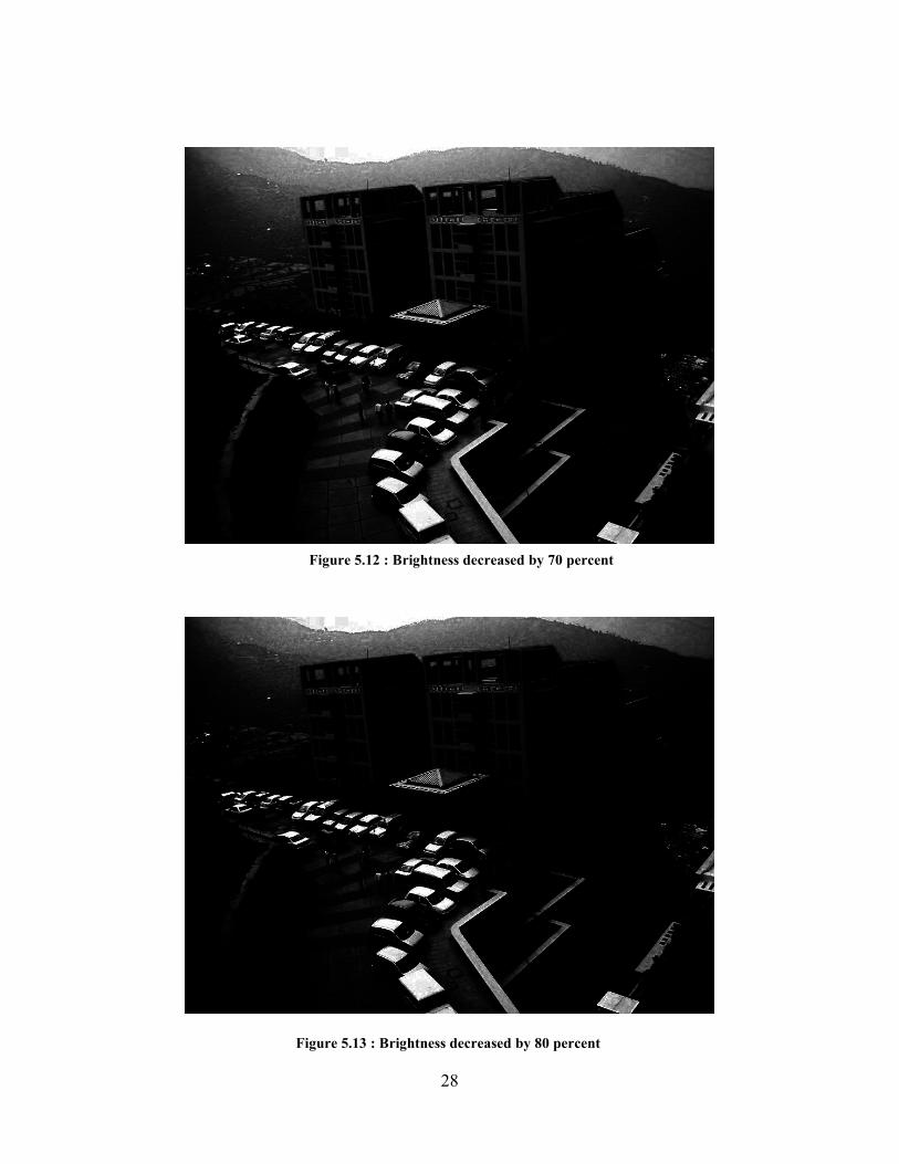
Figure 5.13 : Brightness decreased by 80 percent
Figure 5.12 : Brightness decreased by 70 percent
29
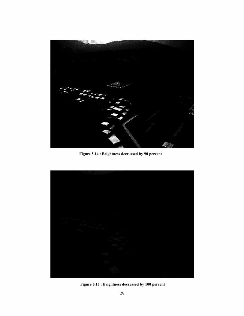
Figure 5.15 : Brightness decreased by 100 percent
Figure 5.14 : Brightness decreased by 90 percent

30
4. Contrast
The variation in the intensity of an image formed by an optical system as
black and white bar. Image contrast is defined as (a-b/a+b) where a and b are
the illuminance in the images of bright and dark bar respectively
4.1 Contrast adjustment
An image lacks contrast when there are no sharp differences between black
and white. Brightness refers to the overall lightness or darkness of an image.
To change the contrast or brightness of an image we perform contrast
stretching. In this process, pixel values below a specified value are displayed as black,
pixel values above a specified value are displayed as white, and pixel values in between
these two values are displayed as shades of gray. The result is a linear mapping of a
subset of pixel values to the entire range of grays, from black to white, producing an
image of higher contrast.
The following figure shows this mapping. Note that the lower limit
and upper limit mark the boundaries of the window, displayed graphically as the red-
tinted window
Fig 5.16 : Relationship of pixel values to display
31
4.2 Contrast Stretching
As mentioned earlier also, contrast stretching (often called normalization) is a
simple image enhancement technique that attempts to improve the contrast in an image
by `stretching' the range of intensity values it contains to span a desired range of values,
e.g. the full range of pixel values that the image type concerned allows. Low contrast
images can be due to the poor illumination, lack of dynamic range in the imaging
sensor, or due to the wrong setting of the lens. The idea behind the contrast stretching is
to increase the dynamic range of intensity level in the processed image
Note: Here we would like to mention that in this project we had to reduce the contrast
and brightness of the image rather than enhancing them. However we utilized
“contrast stretching” technique only but in a opposite manner. In other words we
reduced the range of pixel values rather than increasing it, which gave us the desired
result.

32
CHAPTER -6
EFFECTS OF NIGHT ON AN IMAGE
Here we present some of the examples of final results which we got in the completion
of our project “NIGHT EFFECTS IN AN IMAGE”
8.1 Implementation
Input image was assumed to be RGB image .If it is a high dynamic range image, it
should be scaled to the [0,1] range. Then the image was converted to HSV colormap.
Further the range of pixel values was reduced to [0.2 0.6] and the overall brightness of
the image was reduced by almost 70 percent. The resulting low contrast and low
brightness image is then given a blue shift. Now this bluish image is low pass filtered
using Gaussian Kernel Gkernel where the standard deviation SD1 is chosen to remove the
fine details that would not be visible at night.
I blur = Gkernel * I
The original image is also convolved with second Gaussian Kernel Gkernel2 ,with
standard deviation SD2 =1.6 SD1 after which we take the difference of the two blurred
images.
I blur2 = Gkernel2 * I
Idiff = I blur - I blur2
Idiff is the bandpass component .The final night image was obtained by utilizing the
following equation..
INIGHT = Iblur2 + Idiff0.8

33
Fig 6.1:Day Image 1
Fig 6.2: Night Image 1
34
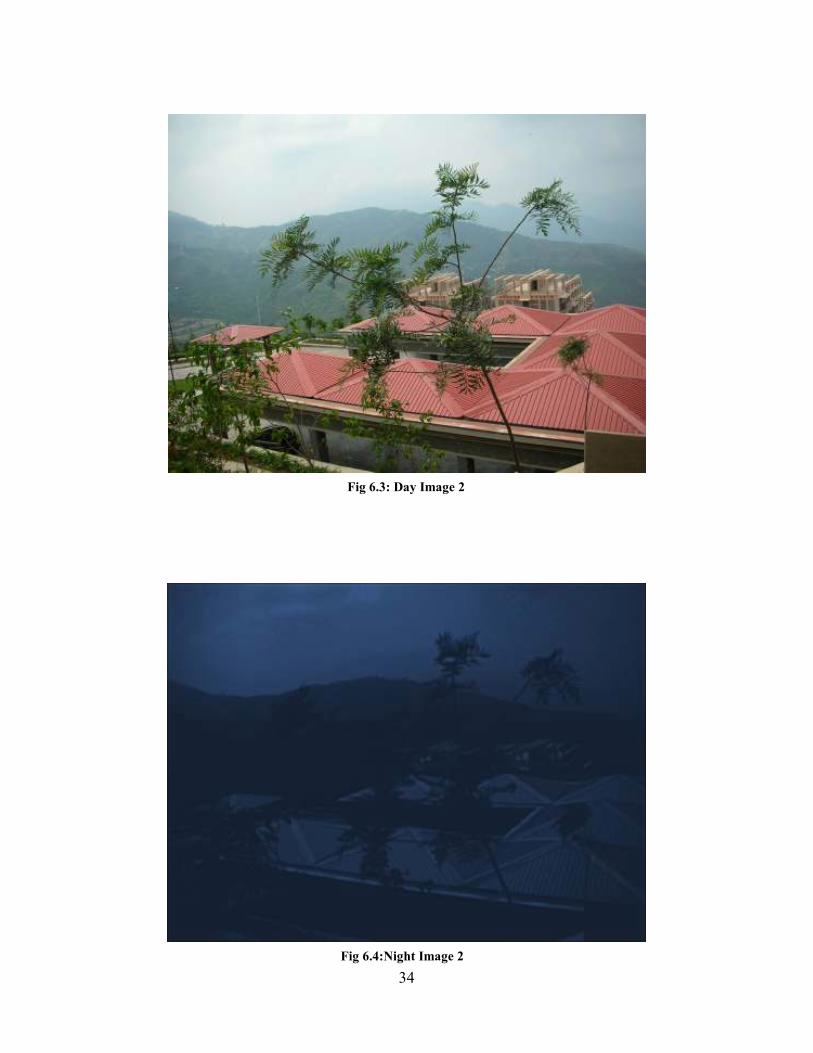
Fig 6.3: Day Image 2
Night Image 2
Fig 6.4:Night Image 2

35
Fig 6.6 :Night Image 3
Fig 6.5: Day Image 3

36
CHAPTER -7
DAWN AND EVENING EFFECTS
An evening image differs from night image in that the evening image has a bit of red
shift along with brightness and contrast reduced by a small percentage. Where as a
dawn image has even less level of brightness and contrast and contains no colour shift.
Fig 7.1: Day Image 1

37
Fig 7.2: Evening image for Fig. 7.1
Fig 7.3: Day image 2

38
Fig 7.4: Dawn image for Fig7.3
39
Conclusion
After the completion of the project we came to the conclusion that an image comprises
of various determining factors which influence the overall view of he image. Variation
in any one factor results major deviation from the original image.Some of the factors
which we analysed during this project includes hue, saturation, brightness and contrast.
However there are still a vast number of aspects which are yet uncovered. The results
which we achieved for the day and night images could be further improved and
researched by studying additional factors like white noise.

40
Bibliography
1 Gonzalez R.C, Woods R.E, Digital Image Processing , Pearson Education
2005
2 Hess, R. F. (1990). Rod-mediated vision: role of post-receptorial filters. InR.
F. Hess, L. T. Sharpe, and K. Nordby (Eds.), Night Vision, pp. 3-
48.Cambridge: Cambridge University Press.
3 Ferwerda J. A, Shirley P, Thompson W. B, A Spatial Post-Processing
Algorithm for. Images of Night Scenes. Peter. University of Utah.
4 Khan S.M ,Pattanaik S.N,Modelling Blue Shift in Moonlight scenes by Rod
Cone intraction.Paper ID: paper_0151, University of California.
5 www.wikipedia.com
6 www.mathworks.com