introducing pietarinen expansion method into …introducing pietarinen expansion method into...

A. ŠvarcRudjer Bošković Institute, Zagreb, Croatia

Introducing Pietarinen expansion method intosingle-channel (!) pole extraction problem

CAMOGLI 2013 / BLED 2015

Mirza Hadžimehmedović, Hedim Osmanović, and Jugoslav StahovUniversity of Tuzla, Tuzla, Bosnia and Herzegovina

1

Lothar Tiator Institut für Kernphyik, Universität Mainz, D-55099 Mainz, Germany

Ron L. WorkmanData Analysis Center at the Institute for Nuclear Studies, Department

of Physics, The George Washington University, Washington, D.C. 20052


Motivation and justification

2

CAMOGLI 2013 / BLED 2015 3

Poles are finally established as the ultimate resonance criterion

1. Conclusions of ATHOS 2012, ATHOS2013

2. Recent change in PDG attitude


Immediate problem:

It is a common knowledge how to extract Breit-Wigner parameters from experimental data,

However, it is rather obscure how to do it with poles

4


We know how to extract Breit-Wigner parameters from experiment because they are defined on the real axes.

(see Camogli Michel)

But, how do we extract pole parameters from experiment because we have to go to the complex energy plane?

5


The usual answer was:

1. Do it globally

One first has to make a model which fits the data, SOLVE IT, and obtain an explicit analytic function in the full complex energy plane. Second, one has to look for the complex poles of the obtained analytic functions.

2. Do it locally

Speed plot, expansions in power series, etc

6

Camogli 2013 / Bled 2015 7

Taylor expansion


Regularization method


In both cases we have n-TH DERIVATIVE of the function

PROBLEMS for local solutions !


Direct problems for global solutions:

• Many models• Complicated and different analytic structure• Elaborated method for solving the problem• SINGLE USER RESULTS


In Camogli 2012, during „coffee-break conversation” I haveclaimed that extracting poles from theoretical and even fromexperimental data should in principle be possible, and I havepromised to try to propose a simple method.

Now I am fulfilling this promise.

13


Is it possible to create universal approach, usable for everyone, and above all REPRODUCIBLE?

I have tryed to do it starting from very general principles:1. Analyticity2. Unitarity

Idea: TRADING ADVANTAGES

GLOBALITY FOR SIMPLICITY


If you create a model, the advantage is that your solution isabsolutely global, valid in the full complex energy plane (allRieman sheets). The drawback is that the solution is complicated,pole positions are usually energy dependent otherwise youcannot ensure simple physical requirements like absence of thepoles on the first, physical Riemann sheet, Schwartz reflectionprinciple, etc. It is complicated and demanding to solve it.

THEORETICAL MODELS

WE PROPOSE

Construct an analytic function NOT in the full complex energy plane, but CLOSE to the real axes in the area of dominant nucleon resonances, which is fitting the data by using

LAURENT EXPANSION.


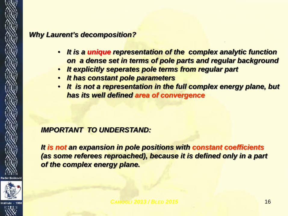
Why Laurent’s decomposition?

• It is a unique representation of the complex analytic function on a dense set in terms of pole parts and regular background

• It explicitly seperates pole terms from regular part• It has constant pole parameters• It is not a representation in the full complex energy plane, but

has its well defined area of convergence

IMPORTANT TO UNDERSTAND:

It is not an expansion in pole positions with constant coefficients (as some referees reproached), because it is defined only in a part of the complex energy plane.


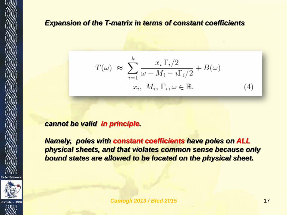
Expansion of the T-matrix in terms of constant coefficients

cannot be valid in principle.

Namely, poles with constant coefficients have poles on ALL physical sheets, and that violates common sense because only bound states are allowed to be located on the physical sheet.


The only way how to accomodateboth, requirements of absence ofpoles on the physical sheet, andSchwartz principle requires thatpole positions become energydependent:

However, even this function has its Laurent decomposition

But it is valid only in the part of the complex energy plane


1. Analyticity

Analyticity is introduced via generalized Laurent’s decomposition(Mittag-Leffler theorem)


Assumption: • We are working with first order poles so all negative powers

in Laurent’s expansion lower than n< -1

are suppressed

Now, we have two parts¸of Laurent’s decomposition:1. Poles 2. Regular part


Idea: TO MIMICK THE PROCEDURE FOR BREIT-WIGNER CASE

Bw:

With Laurent’s decompositions for simple poles

where


The problem is how to determine regular function B(w).

What do we know about it?

�

We know it’s analytic structure for each partial wave!

We do not know its EXPLICT analytic form!


So, instead of „guessing” its exact form by using model assumptions we

EXPAND IT IN FASTLY CONVERGENT POWER SERIES OF PIETARINEN („Z”) FUNCTIONS WITH WELL KNOWN BRANCH-POINTS!

Original idea: 1. S. Ciulli and J. Fischer in Nucl. Phys. 24, 465 (1961)2. I. Ciulli, S. Ciulli, and J. Fisher, Nuovo Cimento 23, 1129

(1962).

Convergence proven in:

1. S. Ciulli and J. Fischer in Nucl. Phys. 24, 465 (1961)2. Detailed proof in I. Caprini and J. Fischer:

"Expansion functions in perturbative QCD and the determination of αs", Phys.Rev. D84 (2011) 054019,

Applied in πN scatteringon the level of invariant

amplitudes PENALTY FUNCTION

INTRODUCED

1. E. Pietarinen, Nuovo Cimento Soc. Ital. Fis. 12A, 522 (1972).

2. Hoehler – Landolt Boernstein „BIBLE” (1983)


What is Pitarinen’s expansion?

In principle, in mathematical language, it is ” ...a conformal mapping which maps the physical sheet of the ω-plane onto the interior of the unit circle in the Z-plane...”In practice this means:


Or in another words, Pietarinen functions Z(ω) are a complet set of functions for an arbitrary function F(ω) which

HAS A BRANCH POINT AT xP !

Observe:

Pietarinen functions do not form a complete set of functions for any function, but only for the function having a well defined branch point.


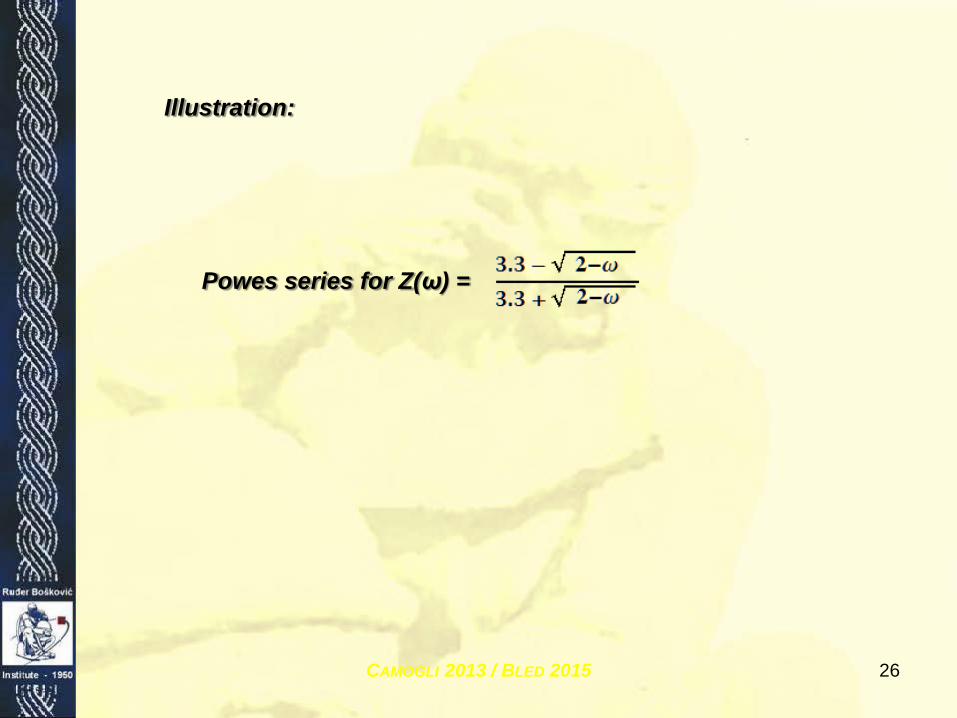
Powes series for Z(ω) =

Illustration:


Z(ω)

4 2 2 4s

0.2

0.4

0.6

0.8

1.0Real

4 2 2 4s

0.8

0.6

0.4

0.2

Imag


Z(ω)2

4 2 2 4s

0.2

0.2

0.4

0.6

0.8

1.0Real

4 2 2 4s

1.0

0.8

0.6

0.4

0.2

Imag


Z(ω)3

4 2 2 4s

1.0

0.5

0.5

1.0Real

4 2 2 4s

1.0

0.8

0.6

0.4

0.2

Imag


Important!A resonance CANNOT be well described by Pietarinen series.

0.5 1.0 1.5 2.0 2.5

1

0

1

2

3

4

5

s

Real

0.5 1.0 1.5 2.0 2.5

0

1

2

3

s

Im

0.5 1.0 1.5 2.0 2.50

1

2

3

4

5

6

sAb

s

xP 4.93028, xQ 1.09731


Courtesy of Lothar Tiator


Finally, the area of convergence for Laurent expansion of P11 partial wave


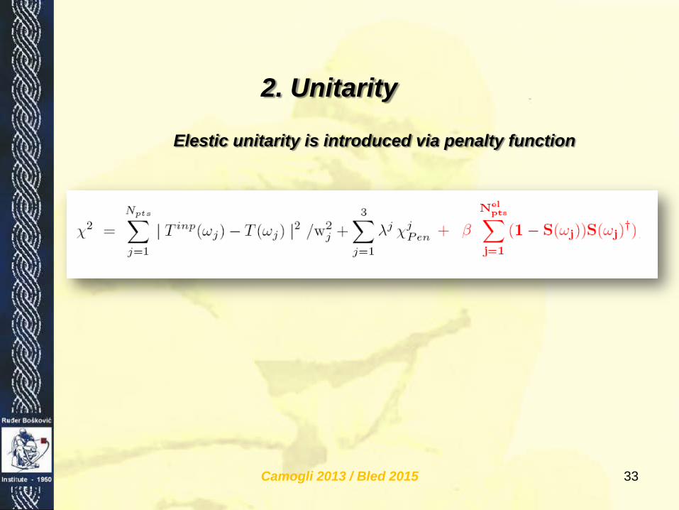
2. Unitarity

Elestic unitarity is introduced via penalty function


Unitarity test


The model


We use Mittag-Leffleur decomposition of „analyzed” function:

k - simple polesregular background

We know analytic properties (number

and position of cuts) of analyzed function

ONE Pietarinen

power seriesper cut


Method has problems, and the one of them definitely is:There is a lot of cuts, so it is difficult to imagine that we shall be able to represent each cut with one Pietarinen series (too many possibly interfering terms).

Answer:We shall use „effective” cuts to represent dominant effects.

We use three Pietarinen series: • One to represent subthreshold, unphysical

contributions• Two in physical region to represent all inelastic

channel openings

Strategy of choosing branchpoint positions is extremely important and will be discussed later


Advantage:

The method is „self-checking” !

It might not work. But, if it works, and if we obtain a good χ2, then we have obtained

AN ANALYTIC FUNCTION WITH WELL KNOWN POLES AND CUTS WHICH DEFINITELY DESCRIBES THE INPUT!

So, if we have disagreements with other methods, then we are looking at two different analytic functions which are almost identical on a discrete set, so we may discuss the general stability of the problem.

However, our solution definitely IS A SOLUTION!


What can we do with this model?

1. We may analyze various kinds of inputs

a. Theoretical curves coming from ANY modelbut also

b. Information coming directly from experiment (partial wave data)

Observe:

To fit „theoretical input” we have to „guess” both: pole position AND analyticity structure of the background

imposed by the analyzed model

To fit „experimental input” we have to „guess” only: pole position AND analyticity structure of the

background as no information about functional type is imposed

Partial wave data are much more convenient to analyze!

40

Does it work?

Testing is a very simple procedure. It comes to:

WorksDoesn’t work

TESTING

a. Testing on a toy model:

b. Testing and application on realistic amplitudes

i. πN elastic scatteringa. ED PW amplitudes (some solutions from GWU/SAID)b. ED PW amplitudes (some solutions from Dubna-Mainz-

Taipei)ii. Photo – and electroproduction on nucleon

a. ED multipoles (all solutions from MAID and SAID)b. SES multipoles (all solutions from MAID and SAID)

arXiv nucl-th 1212.1295



a. Toy model


We have constructed a toy model using two poles and two cuts, used it to construct the input data set, attributed error bars of 5%, and tried to use L+P method to extract pole parameters under different conditions.

C1, C2, B1, B2 = -1, 0, 1


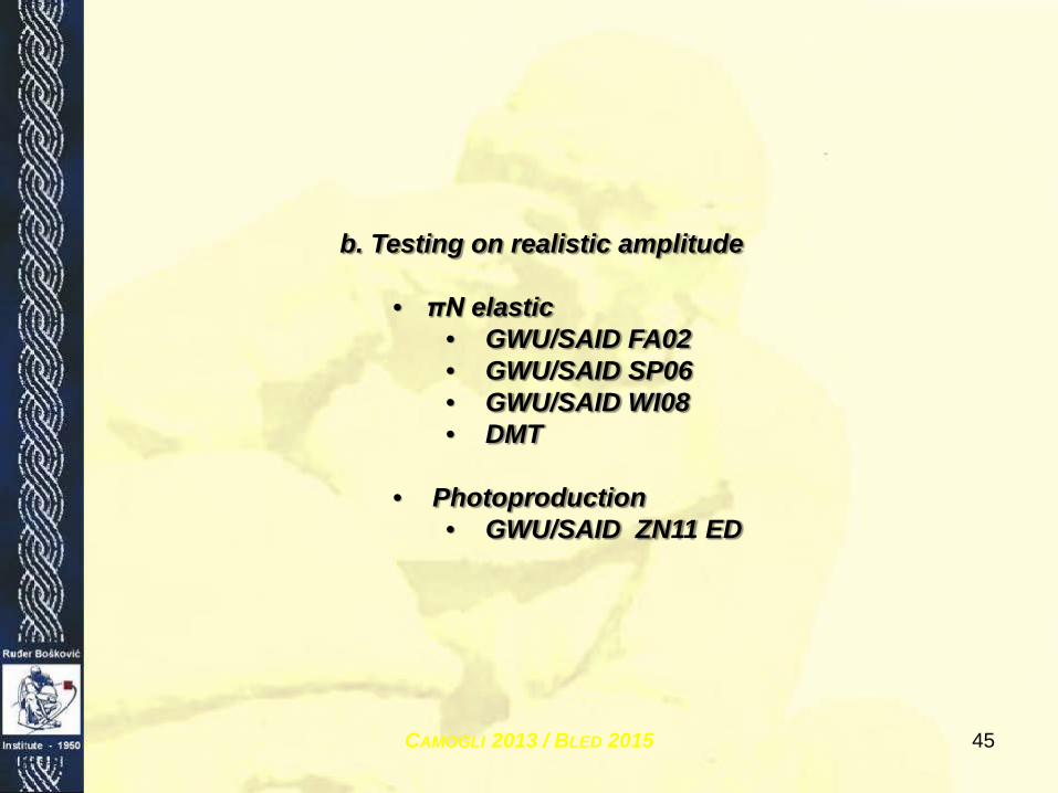
b. Testing on realistic amplitude

• πN elastic• GWU/SAID FA02• GWU/SAID SP06• GWU/SAID WI08• DMT

• Photoproduction• GWU/SAID ZN11 ED


Quality of the fit


πN elastic scatteringSAID FA02 ED


πN elastic scatteringSAID SP06 ED


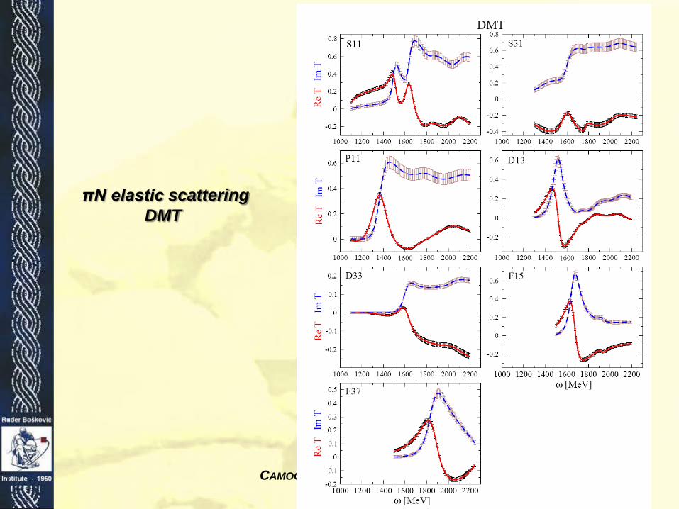
πN elastic scatteringDMT


1785

244

43

-64


Photoproduction


GWU/SAID Zn11 ED solution


XX1785 244


Error analysis


The only problem in the model are thresholds. Their number is definitely at this moment insufficient, so we must propose a stretegy.

Namely, if we fail to reproduce background exactly (and that we certainly do as soon as number of thresholds is insufficient), the pole terms try to compensate for the approximation made.

We propose two strategies:1. To fix the pole at the values expected to dominate for a

chosen channel2. To allow poles to vary as a fitting parameter and allow

the fit to find optimal choice of two effective thresholds which will replace the exact values


In practice this looks like that:

Option 1:

Option 2:


Example of the error estimate:

We used weighted average.


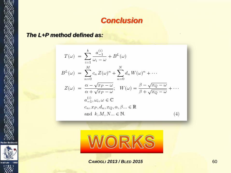
Conclusion

The L+P method defined as:


World recognition

-80-60-40-20

020406080

0 1 2 3 4Q2 (GeV2)

A1/

2 (10

-3G

eV-1

/2)

-40

-20

0

20

40

60

0 1 2 3 4Q2 (GeV2)

S 1/2 (

10-3

GeV

-1/2

)

-100

-75

-50

-25

0

0 2 4Q2 (GeV2)

A1/

2(10

-3G

eV-1

/2)

0

50

100

150

0 2 4Q2 (GeV2)

A3/

2(10

-3G

eV-1

/2)

-80

-60

-40

-20

0

0 2 4Q2 (GeV2)

S 1/2(

10-3

GeV

-1/2

)

0

20

40

60

80

100

120

0 2 4 6

Q2 (GeV2)

A1/

2 (10

-3G

eV-1

/2)

-40

-30

-20

-10

0

10

20

0 1 2 3 4

Q2 (GeV2)

S 1/2 (

10-3

GeV

-1/2

)

Figure 2: Transverse and scalar (longitudi-nal) helicity amplitudes for γp → N(1440)1/2+

(top), γp → N(1520)3/2− (center), and γp →N(1535)1/2− (bottom) as extracted from theJLab/CLAS data in nπ+ production (full cir-cles), in pπ+π− (open triangles), combined sin-gle and double pion production (open squares).The solid triangle is the PDG 2013 value atQ2 = 0. The open boxes are the model uncer-tainties of the full circles. The figures are kindlyprovided by V. Burkert, JLab.

A1/2 is small at the photon point, increases rapidly with Q2

and then falls off with ∼ Q−3. Quantitative agreement with the

data is, however, achieved only when meson cloud effects are

included.

At high Q2, both amplitudes for N(1440)1/2+ are qual-

itatively described by light front quark models [22]: at short

distances the resonance behaves as expected from a radial

excitation of the nucleon. On the other hand, A1/2 changes

sign at about 0.6 GeV2. This remarkable behavior has not been

observed before for any nucleon form factor or transition am-

plitude. Obviously, an important change in the structure occurs

when the resonance is probed as a function of Q2.

The Q2 dependence of A1/2 of the N(1535)1/2− resonance

exhibits the expected ∼ Q−3 dependence, except for small Q2

values where meson cloud effects set in.

VII. Partial wave analyses

Several PWA groups are now actively involved in the anal-

ysis of the new data. The GWU group maintains a nearly

complete database covering reactions from πN and KN elastic

scattering to γN → Nπ, Nη, and Nη′. It is presently the only

group determining πN elastic amplitudes from scattering data

in sliced energy bins. Given the high-precision of photoproduc-

tion data already or soon to be collected, the spectrum of N

and Δ resonances will in the near future be better known.

Fits to the data are performed by various groups with the

aim to understand the reaction dynamics and to identify N

and Δ resonances. For practical reasons, approximations have

to be made. We mention several analyses here: (1) The Mainz

unitary isobar model [23] focusses on the correct treatment of

the low-energy domain. Resonances are added to the unitary

amplitude as a sum of Breit-Wigner amplitudes. This model

also obtains resonance transition form factors and helicity

amplitudes from electroproduction [19]. (2) For Nπ electro-

production, the Yerevan/JLab group uses both the unitary

isobar model and the dispersion relation approach developed

in [22]. A phenomenological model was developed to extract

resonance couplings and partial decay widths from exclusive

π+π−p electroproduction [21]. (3) Multichannel analyses us-

ing K-matrix parameterizations derive background terms from

a chiral Lagrangian - providing a microscopical description of

the background - (Giessen [24,25]) or from phenomenology

(Bonn-Gatchina [26]) . (4.) Several groups (EBAC-Jlab [27,28],

ANL-Osaka [29], Dubna-Mainz-Taipeh [30], Bonn-Julich

[31,32,33], Valencia [34]) use dynamical reaction models,

driven by chiral Lagrangians, which take dispersive parts of in-

termediate states into account. Several other groups have made

important contributions. The Giessen group pioneered multi-

channel analyses of large data sets on pion- and photo-induced

reactions [24,25]. The Bonn-Gatchina group included recent

high-statistics data and reported systematic searches for new

baryon resonances in all relevant partial waves. A summary of

their results can be found in Ref. [26].

References

1. G. Hohler, Pion-Nucleon Scattering, Landolt-BornsteinVol. I/9b2 (1983), ed. H. Schopper, Springer Verlag.

2. R.E. Cutkosky et al., Baryon 1980, IV International Con-

ference on Baryon Resonances, Toronto, ed. N. Isgur,p. 19.

3. R.A. Arndt et al., Phys. Rev. C74, 045205 (2006).

4. Hadron 2011: 14th International Conference on Hadron

Spectroscopy, Munchen, Germany, June, 13 - 17, 2011,published in eConf.

5. NSTAR 2013: 9th International Workshop on the Physics

of Excited Nucleons, 27-30 May 2013, Peniscola, Spain.

6. E. Klempt and J.M. Richard, Rev. Mod. Phys. 82, 1095(2010).

7. V. Crede and W. Roberts, Rept. Prog. Phys. 76, 076301(2013).

8. M. Roos et al., Phys. Lett. B111, 1 (1982).

9. A. Svarc et al., Phys. Rev. C88, 035206 (2013).

10. R.H. Dalitz and R.G. Moorhouse, Proc. Roy. Soc. Lond.A318, 279 (1970).

11. C. G. Fasano et al., Phys. Rev. C46, 2430 (1992).

12. G.F. Chew et al., Phys. Rev. 106, 1345 (1957).

13. R. L. Workman, L. Tiator, and A. Sarantsev, Phys. Rev.C87, 068201 (2013).

14. N. Suzuki, T. Sato, and T. -S. H. Lee, Phys. Rev. C82,045206 (2010).

9. A. Svarc et al., Phys. Rev. C888, 035206 (2013).


A. Švarc and L. Tiator

Publication

introducing pietarinen expansion method into …introducing pietarinen expansion method into...

Documents