1

Introduction

The history of error correcting coding (ECC) started with the introduction of the Hammingcodes (Hamming 1974), at or about the same time as the seminal work of Shannon (1948).Shortly after, Golay codes were invented (Golay 1974). These two first classes of codesare optimal, and will be defined in a subsequent section.

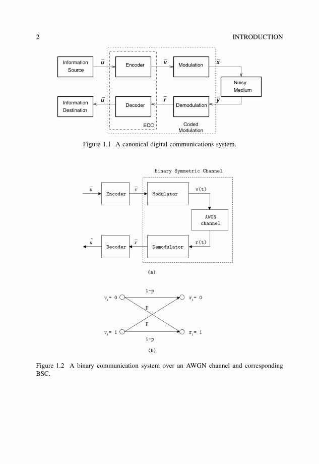
Figure 1.1 shows the block diagram of a canonical digital communications/storagesystem. This is the famous Figure 1 in most books on the theory of ECC and digitalcommunications (Benedetto and Biglieri 1999). The information source and destinationwill include any source coding scheme matched to the nature of the information. The ECCencoder takes as input the information symbols from the source and adds redundant sym-bols to it, so that most of the errors – introduced in the process of modulating a signal,transmitting it over a noisy medium and demodulating it – can be corrected (Massey 1984;McEliece 1977; Moon 2005).

Usually, the channel is assumed to be such that samples of an additive noise processare added to the modulated symbols (in their equivalent complex baseband representation).The noise samples are assumed to be independent from the source symbols. This model isrelatively easy to track mathematically and includes additive white Gaussian noise (AWGN)channels, flat Rayleigh fading channels, and binary symmetric channels (BSC). The case offrequency-selective channels can also be included, as techniques such as spread-spectrumand multicarrier modulation (MCM) effectively transform them into either AWGN channelsor flat Rayleigh fading channels.

At the receiver end, the ECC decoder utilizes the redundant symbols and their rela-tionship with the information symbols in order to correct channel errors. In the case oferror detection, the ECC decoder can be best thought of as a reencoder of the receivedinformation, followed by a check that the redundant symbols generated are the same asthose received.

In classical ECC theory, the combination of modulation, noisy medium and demod-ulation was modeled as a discrete memoryless channel with input v and output r .An example of this is binary transmission over an AWGN channel, which is modeledas a BSC. This is illustrated in Figure 1.2. The BSC has a probability of channelerror p – or transition probability – equal to the probability of a bit error for binary

The Art of Error Correcting Coding Second Edition Robert H. Morelos-Zaragoza 2006 John Wiley & Sons, Ltd

COPYRIG

HTED M

ATERIAL

2 INTRODUCTION

_

_

_

_

_

~

Encoder

Decoder Demodulation

Noisy

Medium

Information

Source

Destination

Information

u v x

yru

Modulation

ModulationCodedECC

Figure 1.1 A canonical digital communications system.

Encoderu

u r

vModulator

AWGN

channel

Decoder Demodulator

^

Binary Symmetric Channel

v(t)

r(t)

(a)

(b)

vi

i

i

i

= 0

v = 1

r = 0

r = 1

p

p

1−p

1−p

Figure 1.2 A binary communication system over an AWGN channel and correspondingBSC.

INTRODUCTION 3

signaling over an AWGN channel,

p = Q

(√2Eb

N0

), (1.1)

where Eb/N0 is the energy-per-bit-to-noise ratio – also referred to as the bit signal-to-noiseratio (SNR) or SNR per bit – and

Q(x) = 1√2π

∫ ∞

x

e−z2/2 dz, (1.2)

is the Gaussian Q-function. In terms of the complementary error function, the Q-functioncan be written as

Q(x) = 1

2erfc

(x√2

). (1.3)

Equation (1.2) is useful in analytical derivations and Equation (1.3) is used in the compu-tation with C programs or Matlab scripts of performance bounds and approximations.

Massey (1974) suggested considering ECC and modulation as a single entity, knownin modern literature as coded modulation. This approach provides a higher efficiency andcoding gain1 rather than the serial concatenation of ECC and modulation, by joint design ofcodes and signal constellations. Several methods of combining coding and modulation arecovered in this book, including the following: trellis-coded modulation (TCM) (Ungerboeck1982) and multilevel coded modulation (MCM) (Imai and Hirakawa 1977). In a coded mod-ulation system, the (soft-decision) channel outputs are directly processed by the decoder.In contrast, in a classical ECC system, the hard-decision bits from the demodulator are fedto a binary decoder.

Codes can be combined in several ways. An example of serial concatenation (that is,concatenation in the classical sense) is the following. For years, the most popular con-catenated ECC scheme has been the combination of an outer Reed–Solomon (RS) code,through intermediate interleaving, and an inner binary convolutional code. This scheme hasbeen used in numerous applications, ranging from space communications to digital broad-casting of high definition television. The basic idea is that the soft-decision decoder of theconvolutional code produces bursts of errors that can be broken into smaller pieces by thedeinterleaving process and handled effectively by the RS decoder. RS codes are nonbinarycodes that work with symbols composed of several bits, and can deal with multiple burstsof errors. Serial concatenation has the advantage that it requires two separate decoders,one for the inner code and one for the outer code, instead of a single but very complexdecoder for the overall code.

This book examines these types of ECC systems. First, basic code constructions andtheir decoding algorithms, in the Hamming space (that is, dealing with bits), are presented.In the second part of the book, important soft-decision decoding (SDD) algorithms forbinary transmission are introduced. These algorithms work over the Euclidean space andachieve a reduction in the required transmitted power per bit of at least 2 dB, comparedwith Hamming-space (hard-decision) decoders. Several kinds of soft-decision decoders are

1Coding gain is defined as the difference in SNR between the coded system and an uncoded system with thesame bit rate.

4 INTRODUCTION

considered, with attention given to their algorithmic aspects (the “how” they work), ratherthan to their theoretical aspects (the ‘why’ they work). Finally, combinations of codes andinterleaving for iterative decoding and of coding and modulation for bandwidth-efficienttransmission are the topic of the last part of the book.

1.1 Error correcting coding: Basic concepts

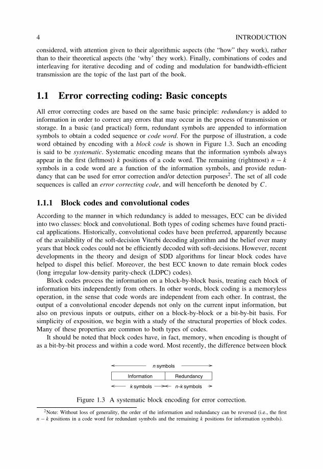
All error correcting codes are based on the same basic principle: redundancy is added toinformation in order to correct any errors that may occur in the process of transmission orstorage. In a basic (and practical) form, redundant symbols are appended to informationsymbols to obtain a coded sequence or code word. For the purpose of illustration, a codeword obtained by encoding with a block code is shown in Figure 1.3. Such an encodingis said to be systematic. Systematic encoding means that the information symbols alwaysappear in the first (leftmost) k positions of a code word. The remaining (rightmost) n − k

symbols in a code word are a function of the information symbols, and provide redun-dancy that can be used for error correction and/or detection purposes2. The set of all codesequences is called an error correcting code, and will henceforth be denoted by C.

1.1.1 Block codes and convolutional codes

According to the manner in which redundancy is added to messages, ECC can be dividedinto two classes: block and convolutional. Both types of coding schemes have found practi-cal applications. Historically, convolutional codes have been preferred, apparently becauseof the availability of the soft-decision Viterbi decoding algorithm and the belief over manyyears that block codes could not be efficiently decoded with soft-decisions. However, recentdevelopments in the theory and design of SDD algorithms for linear block codes havehelped to dispel this belief. Moreover, the best ECC known to date remain block codes(long irregular low-density parity-check (LDPC) codes).

Block codes process the information on a block-by-block basis, treating each block ofinformation bits independently from others. In other words, block coding is a memorylessoperation, in the sense that code words are independent from each other. In contrast, theoutput of a convolutional encoder depends not only on the current input information, butalso on previous inputs or outputs, either on a block-by-block or a bit-by-bit basis. Forsimplicity of exposition, we begin with a study of the structural properties of block codes.Many of these properties are common to both types of codes.

It should be noted that block codes have, in fact, memory, when encoding is thought ofas a bit-by-bit process and within a code word. Most recently, the difference between block

Information

k symbols

Redundancy

n-k symbols

n symbols

Figure 1.3 A systematic block encoding for error correction.

2Note: Without loss of generality, the order of the information and redundancy can be reversed (i.e., the firstn − k positions in a code word for redundant symbols and the remaining k positions for information symbols).

INTRODUCTION 5

and convolutional codes has become less and less well defined, especially after recentadvances in the understanding of the trellis structure of block codes, and the tail-bitingstructure of some convolutional codes. Indeed, colleagues working on convolutional codessometimes refer to block codes as “codes with time-varying trellis structure.” Similarly,researchers working with block codes may consider convolutional codes as “codes with aregular trellis structure.”

1.1.2 Hamming distance, Hamming spheres and errorcorrecting capability

Consider an error correcting code C with binary elements. As mentioned above, block codesare considered for simplicity of exposition. In order to achieve error correcting capabilities,not all the 2n possible binary vectors of length n are allowed to be transmitted. Instead, C

is a subset of the n-dimensional binary vector space V2 = {0, 1}n, such that its elementsare as far apart as possible.

Consider two vectors x1 = (x1,0, x1,1, . . . , x1,n−1) and x2 = (x2,0, x2,1, . . . , x2,n−1) inV2. Then the Hamming distance between x1 and x2, denoted dH (x1, x2), is defined as thenumber of elements in which the vectors differ,

dH (x1, x2)�= ∣∣ {i : x1,i �= x2,i , 0 ≤ i < n

} ∣∣ =n−1∑i=0

x1,i ⊕ x2,i , (1.4)

where |A| denotes the number of elements in (or the cardinality of) a set A and ⊕ denotesaddition modulo-2 (exclusive-OR).

Given a code C, its minimum Hamming distance, dmin, is defined as the minimumHamming distance among all possible distinct pairs of code words in C,

dmin = minv1,v2∈C

{dH (v1, v2)|v1 �= v2} . (1.5)

Throughout the book, the array (n, k, dmin) is used to denote the parameters of a blockcode of length n, that encodes messages of length k bits and has a minimum Hammingdistance dmin. The assumption is made that the size of the code is |C| = 2k .

Example 1.1.1 The simplest error correcting code is a binary repetition code of length 3.It repeats each bit three times, so that a “0” is encoded onto the vector (000) and a “1”onto the vector (111). Since the two code words differ in all three positions, the Hammingdistance between them is equal to three. Figure 1.4 is a pictorial representation of thiscode. The three-dimensional binary space corresponds to the set of 23 = 8 vertices of thethree-dimensional unit-volume cube. The Hamming distance between code words (000) and(111) equals the number of edges in a path between them. This is equivalent to the numberof coordinates that one needs to change to convert (000) into (111), or vice versa. ThusdH ((000), (111)) = 3. There are only two code words in this case, as a result, dmin = 3.

The binary vector space V2 is also known as a Hamming space. Let v denote a codeword of an error correcting code C. A Hamming sphere St (v), of radius t and centeredaround v, is the set of vectors in V2 at a distance less than or equal to t from the center v,

St (v) = {x ∈ V2|dH (x, v) ≤ t} . (1.6)

6 INTRODUCTION

xx

x

0

1

2

Figure 1.4 A (3,1,3) repetition code in a three-dimensional binary vector space.

Note that the size of (or the number of code words in) St (v) is given by the followingexpression ∣∣St (v)

∣∣ =t∑

i=0

(n

i

). (1.7)

Example 1.1.2 Figure 1.5 shows the Hamming spheres of radius t = 1 around the codewords of the (3, 1, 3) binary repetition code.

Note that the Hamming spheres for this code are disjoint, that is, there is no vector inV2 (or vertex in the unit-volume three-dimensional cube) that belongs to both S1(000) andS1(111). As a result, if there is a change in any one position of a code word v, then theresulting vector will still lie inside a Hamming sphere centered at v. This concept is thebasis of understanding and defining the error correcting capability of a code C.

The error correcting capability, t , of a code C is the largest radius of Hamming spheresSt (v) around all the code words v ∈ C, such that for all different pairs vi , vj ∈ C, thecorresponding Hamming spheres are disjoint, that is,

t = maxvi ,vj∈C

{�|S�(vi) ∩ S�(vj ) = ∅, vi �= vj

}. (1.8)

In terms of the minimum distance of C, dmin, an equivalent and more common definitionis

t = (dmin − 1)/2, (1.9)

where x denotes the largest integer less than or equal to x.

xx

x

0

1

2

xx

x

0

1

2

S1 (111)S1 (000)

Figure 1.5 Hamming spheres of radius t = 1 around the code words of the (3,1,3) binaryrepetition code.

INTRODUCTION 7

Note that in order to compute the minimum distance dmin of a block code C, in accor-dance with Equation (1.5), a total of 2k−1(2k − 1) distances between distinct pairs of codewords are needed. This is practically impossible even for codes of relatively modest size,say, k = 50 (for which approximately 299 code word pairs need to be examined). One ofthe advantages of linear block codes is that the computation of dmin requires to know theHamming weight of all 2k − 1 nonzero code words.

1.2 Linear block codes

As mentioned above, finding a good code means finding a subset of V2 with elements asfar apart as possible. This is very difficult. In addition, even when such a set is found, thereis still the problem of how to assign code words to information messages.

Linear codes are vector subspaces of V2. This means that encoding can be accomplishedby matrix multiplications. In terms of digital circuitry, simple encoders can be built usingexclusive-OR gates, AND gates and D flip-flops. In this chapter, the binary vector spaceoperations of sum and multiplication are meant to be the output of exclusive-OR (or modulo2 addition) and AND gates, respectively. The tables of addition and multiplication for thebinary elements in {0, 1} are as follows:

a b a + b a · b

0 0 0 00 1 1 01 0 1 01 1 0 1

which are seen to correspond to the outputs of a binary exclusive-OR gate and an ANDgate, respectively.

1.2.1 Generator and parity-check matrices

Let C denote a binary linear (n, k, dmin) code. Now, C is a k-dimensional vector subspace,and therefore it has a basis, say {v0, v1, . . . , vk−1}, such that any code word v ∈ C can berepresented as a linear combination of the elements on the basis of:

v = u0v0 + u1v1 + · · · + uk−1vk−1, (1.10)

where ui ∈ {0, 1}, 1 ≤ i < k. Equation (1.10) can be written in terms of a generator matrixG and a message vector, u = (u0, u1, . . . , uk−1), as follows:

v = uG, (1.11)

where

G =

v0

v1...

vk−1

=

v0,0 v0,1 · · · v0,n−1

v1,0 v1,1 · · · v1,n−1...

.... . .

...

vk−1,0 vk−1,1 · · · vk−1,n−1

. (1.12)

8 INTRODUCTION

Due to the fact that C is a k-dimensional vector space in V2, there is an (n − k)-dimensionaldual space C�, generated by the rows of a matrix H , called the parity-check matrix, suchthat GH� = 0, where H� denotes the transpose of H . In particular, note that for any codeword v ∈ C,

vH� = 0. (1.13)

Equation (1.13) is of fundamental importance in decoding of linear codes, as will be shownin section 1.3.2.

A linear code C⊥ that is generated by H is a binary linear (n, n − k, d⊥min) code, called

the dual code of C.

1.2.2 The weight is the distance

As mentioned in section 1.1.2, a nice feature of linear codes is that computing the minimumdistance of the code amounts to computing the minimum Hamming weight of its nonzerocode words. In this section, this fact is shown. The Hamming weight, wtH (x), of a vectorx = (x0, x1, . . . , xn−1) ∈ V2 is defined as the number of nonzero elements in x, which canbe expressed as the sum

wtH (x) =n−1∑i=0

xi . (1.14)

From the definition of the Hamming distance, it is easy to see that wtH (x) = dH (x, 0). Fora binary linear code C, note that the distance

dH (v1, v2) = dH (v1 + v2, 0) = wtH (v1 + v2) = wtH (v3), (1.15)

where, by linearity, v1 + v2 = v3 ∈ C. As a consequence, the minimum distance of C canbe computed by finding the minimum Hamming weight among the 2k − 1 nonzero codewords. This is simpler than the brute force search among all the pairs of code words,although still a considerable task even for codes of modest size (or dimension k).

1.3 Encoding and decoding of linear block codes

1.3.1 Encoding with G and H

Equation (1.11) gives an encoding rule for linear block codes that can be implemented ina straightforward way. If encoding is to be systematic, then the generator matrix G of alinear block (n, k, dmin) code C can be brought to a systematic form, Gsys, by elementaryrow operations and/or column permutations. Gsys is composed of two submatrices: Thek-by-k identity matrix, denoted Ik , and a k-by-(n − k) parity submatrix P , such that

Gsys = (Ik|P

), (1.16)

where

P =

p0,0 p0,1 · · · p0,n−k−1

p1,0 p1,1 · · · p1,n−k−1...

.... . .

...

pk−1,0 pk−1,1 · · · pk−1,n−k−1

. (1.17)

INTRODUCTION 9

Since GH� = 0k,n−k, where 0k,n−k denotes the k-by-(n − k) all-zero matrix, it follows thatthe systematic form, Hsys, of the parity-check matrix is

Hsys = (P �|In−k

). (1.18)

Example 1.3.1 Consider a binary linear (4, 2, 2) code with generator matrix

G =(

1 1 1 00 0 1 1

).

To bring G into systematic form, permute (exchange) the second and fourth columns andobtain

Gsys =(

1 0 1 10 1 1 0

).

Thus, the parity-check submatrix is given by

P =(

1 11 0

).

It is interesting to note that in this case, the relation P = P � holds3. From (1.18) it followsthat the systematic form of the parity-check matrix is

Hsys =(

1 1 1 01 0 0 1

).

In the following, let u = (u0, u1, . . . , uk−1) denote an information message to beencoded and v = (v0, v1, . . . , vn−1) the corresponding code word in C.

If the parameters of C are such that k < (n − k), or equivalently the code ratek/n < 1/2, then encoding with the generator matrix is the most economical. The costconsidered here is in terms of binary operations. In such a case

v = uGsys = (u, vp), (1.19)

where vp = uP = (vk, vk+1, . . . , vn−1) represents the parity-check (redundant) part of thecode word.

However, if k > (n − k), or k/n > 1/2, then alternative encoding with the parity-checkmatrix H requires less number of computations. In this case, we have encoding based onEquation (1.13), (u, vp)H� = 0, such that the (n − k) parity-check positions vk, vk+1, . . .,vn−1 are obtained as follows:

vj = u0p0,j + u1p1,j + · · · + uk−1pk−1,j , k ≤ j < n. (1.20)

Stated in other terms, the systematic form of a parity-check matrix of a linear code hasas entries of its rows the coefficients of the parity-check equations, from which the valuesof the redundant positions are obtained. This fact will be used when LDPC codes arepresented, in Section 8.3.

3In this case, the code in question is referred to as a self-dual code. See also Section 2.2.3.

10 INTRODUCTION

Example 1.3.2 Consider the binary linear (4, 2, 2) code from Example 1.3.1. Let messagesand code words be denoted by u = (u0, u1) and v = (v0, v1, v2, v3), respectively. From(1.20) it follows that

v2 = u0 + u1

v3 = u0

The correspondence between the 22 = 4 two-bit messages and code words is as follows:

(00) → (0000)

(01) → (0110)

(10) → (1011)

(11) → (1101) (1.21)

1.3.2 Standard array decoding

In this section, a decoding procedure is presented that finds the closest code word v toa received noisy word r = v + e. The error vector e ∈ {0, 1}n is produced by a BSC, asdepicted in Figure 1.6. It is assumed that the crossover probability (or BSC parameter) p

is such that p < 1/2.As shown in Table 1.1 a standard array (Slepian 1956) for a binary linear (n, k, dmin)

code C is a table of all possible received vectors r arranged in such a way that theclosest code word v to r can be read out. The standard array contains 2n−k rows and 2k + 1columns. The entries of the rightmost 2k columns of the array contain all the vectors inV2 = {0, 1}n.

In order to describe the decoding procedure, the concept of syndrome is needed. Thesyndrome of a word in V2 is defined from Equation (1.13) as

s = rH�, (1.22)

0

1

0

1

Sent Received

1-p

p

p

1-p

Figure 1.6 A binary symmetric channel model.

Table 1.1 The standard array of a binary linear block code.

s u0 = 0 u2 · · · uk−1

0 v0 = 0 v1 · · · v2k−1s1 e1 e1 + v1 · · · e1 + v2k−1s2 e2 e2 + v1 · · · e2 + v2k−1...

......

. . ....

s2n−k−1 e2n−k−1 e2n−k−1 + v1 · · · e2n−k−1 + v2k−1

INTRODUCTION 11

where H is the parity-check matrix of C. That s is indeed a set of symptoms that indicateerrors is shown as follows. Suppose that a code word v ∈ C is transmitted over a BSC andreceived as r = v + e. The syndrome of r is

s = rH� = (v + e)H� = eH�, (1.23)

where to obtain the last equality Equation (1.13) has been used. Therefore, the computationof the syndrome can be thought of as a linear transformation of an error vector.

Standard array construction procedure

1. As the first row, in the positions corresponding to the 2k rightmost columns, enter allthe code words of C, beginning with the all-zero code word in the leftmost position.In the position corresponding to the first column, enter the all-zero syndrome. Letj = 0.

2. Let j = j + 1. Find the smallest Hamming weight word ej in V2, not in C, andnot included in previous rows. The corresponding syndrome sj = ejH

� is the first(rightmost) entry of the row. The 2k remaining entries in that row are obtained byadding ej to all the entries in the first row (the code words of C).

3. Repeat the previous step until all vectors in V2 are included in the array. Equivalently,let j = j + 1. If j < 2n−k, then repeat previous step, otherwise stop.

Example 1.3.3 The standard array of the binary linear (4, 2, 2) code is the following:

s 00 01 10 11

00 0000 0110 1011 110111 1000 1110 0011 010110 0100 0010 1111 100101 0001 0111 1010 1100

Decoding with the standard array proceeds as follows. Let r = v + e be the receivedword. Find the word in the array and output as decoded message u the header of the columnin which r lies. Conceptually, this process requires storing the entire array and matchingthe received word to an entry in the array.

However, a simplified decoding procedure can be found by noticing that every row inthe array has the same syndrome. Each row of the array, denoted Rowi , with 0 ≤ i < 2n−k ,a coset of C, is such that Rowi = {

ei + v∣∣v ∈ C

}. The vector ei is known as the coset

leader.The syndrome of the elements in the i-th row is given by

si = (ei + v)H� = eiH�, (1.24)

which is independent of the particular choice of v ∈ C. The simplified decoding procedureis: compute the syndrome of the received word r = ei′ + v,

si′ = (ei′ + v) H� = ei′H�,

12 INTRODUCTION

and find si′ in the leftmost column of the standard array. Then read out the value of ei′ ,from the second column, and add it to the received word to obtain the closest code wordv′ ∈ C to r . Therefore instead of n × 2n bits, standard array decoding can be implementedwith an array of n × 2n−k bits.

Example 1.3.4 Consider again the binary linear (4, 2, 2) code from Example 1.3.1. Supposethat the code word v = (0110) is transmitted and that r = (0010) is received. Then thesyndrome is

s = rH� = (0010)

1 11 01 00 1

= (

1 0).

From the standard array of the code, the corresponding coset leader e′ = (0100) is found,and therefore, the estimated code word is v′ = r + e′ = (0010) + (0100) = (0110). Oneerror has been corrected! This may sound strange, since the minimum distance of the codeis only two, and thus according to (1.9) single error, correction is impossible. However, thiscan be explained by looking again at the standard array of this code (Example 1.3.3 above).Note that the third row of the array contains two distinct binary vectors of weight one. Thismeans that only three out of a total of four single-error patterns can be corrected. The errorabove is one of those correctable single-error patterns.

It turns out that this (4, 2, 2) code is the simplest instance of a linear Linear unequalerror protection (LUEP) code (van Gils 1983; Wolf and Viterbi 1996). This LUEP code hasa separation vector s = (3, 2), which means that the minimum distance between any twocode words for which the first message bit differs is at least three, and that for the secondmessage bit is at least two.

If encoding is systematic, then the above procedure gives the estimated message u′ inthe first k positions of v′. This is a plausible reason for having a systematic encoding.

1.3.3 Hamming spheres, decoding regions and the standard array

The standard array is also a convenient way of understanding the concept of Hammingsphere and error correcting capability of a linear code C, introduced in Section 1.1.2.

By construction, note that the 2k rightmost columns of the standard array, denoted Colj ,for 1 ≤ j ≤ 2k , contain a code word vj ∈ C and a set of 2n−k − 1 words at the smallestHamming distance from vj , that is,

Colj = {vj + ei

∣∣ei ∈ Rowi , 0 ≤ i < 2n−k}. (1.25)

The sets Colj are known as the decoding regions, in the Hamming space, around each codeword vj ∈ C, for 0 ≤ j ≤ 2k − 1. This is to say that if code word vj ∈ C is transmittedover a BSC and the received word r lies in the set Colj , then it will be successfully decodedinto vj .

Hamming bound

The set Colj and the error correcting capability t of code C are related by the Hammingsphere St (vj ): A binary linear (n, k, dmin) code C has decoding regions Colj that properlycontain Hamming spheres St (vj ), that is, St (vj ) ⊆ Colj .

INTRODUCTION 13

By noticing that the size of Colj is 2n−k, and using Equation (1.7), we obtain thecelebrated Hamming bound

t∑i=0

(n

i

)≤ 2n−k. (1.26)

The Hamming bound has several combinatorial interpretations. One of them is:

The number of syndromes, 2n−k , must be greater than or equal to the numberof correctable error patterns,

∑ti=0

(ni

).

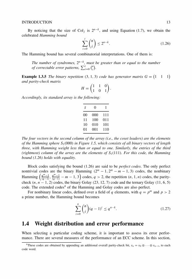
Example 1.3.5 The binary repetition (3, 1, 3) code has generator matrix G = (1 1 1

)and parity-check matrix

H =(

1 1 01 0 1

).

Accordingly, its standard array is the following:

s 0 1

00 000 11111 100 01110 010 10101 001 110

The four vectors in the second column of the array (i.e., the coset leaders) are the elementsof the Hamming sphere S1(000) in Figure 1.5, which consists of all binary vectors of lengththree, with Hamming weight less than or equal to one. Similarly, the entries of the third(rightmost) column of the array are the elements of S1(111). For this code, the Hammingbound (1.26) holds with equality.

Block codes satisfying the bound (1.26) are said to be perfect codes. The only perfectnontrivial codes are the binary Hamming (2m − 1, 2m − m − 1, 3) codes, the nonbinary

Hamming(

qm−1(q−1)

,qm−1(q−1)

− m − 1, 3)

codes, q > 2, the repetition (n, 1, n) codes, the parity-check (n, n − 1, 2) codes, the binary Golay (23, 12, 7) code and the ternary Golay (11, 6, 5)

code. The extended codes4 of the Hamming and Golay codes are also perfect.For nonbinary linear codes, defined over a field of q elements, with q = pm and p > 2

a prime number, the Hamming bound becomes

n∑i=0

(n

i

)(q − 1)i ≤ qn−k. (1.27)

1.4 Weight distribution and error performance

When selecting a particular coding scheme, it is important to assess its error perfor-mance. There are several measures of the performance of an ECC scheme. In this section,

4These codes are obtained by appending an additional overall parity-check bit, vn = v0 ⊕ · · · ⊕ vn−1, to eachcode word.

14 INTRODUCTION

expressions for linear codes are introduced, for three basic channel models: The BSC model,the AWGN channel model and the flat Rayleigh fading channel model.

1.4.1 Weight distribution and undetected error probabilityover a BSC

The weight distribution W(C) of an error correcting code C, is defined as the set of n + 1integers W(C) = {Ai, 0 ≤ i ≤ n}, such that there are Ai code words of Hamming weighti in C, for i = 0, 1, . . . , n.

An expression for the probability of undetected error of a linear code over a BSC isderived next. First, note that the Hamming weight of a word v, wtH (v) equals the Hammingdistance to the all-zero word, wtH (v) = dH (v, 0). Also, as noted before, the Hammingdistance between any two code words v1, v2 in a linear code C equals the Hamming weightof their difference,

dH (v1, v2) = dH (v1 + v2, 0) = wtH (v1 + v2) = wtH (v3),

where, by linearity of C, v3 ∈ C.The probability of an undetected error, denoted Pu(C), is the probability that the

received word differs from the transmitted code word but the syndrome equals zero. Thatis,

s = (v + e)H� = eH� = 0 ⇐⇒ e ∈ C.

Therefore, the probability that the syndrome of the received word is zero equals the prob-ability that an error vector is a nonzero code word in C.

With transmission over a BSC, the probability that the error vector e has weight i

equals the probability that i bits are in error and that the remaining n − i bits are correct.Let P (e, i) denote this probability. Then

P (e, i) = pi(1 − p)n−i .

For an undetected error to occur, the error vector e must be a nonzero code word. Thereare Ai vectors of weight i in C. It follows that

Pu(C) =n∑

i=dmin

Ai P (e, i) =n∑

i=dmin

Ai pi(1 − p)n−i . (1.28)

Equation (1.28) gives the exact value of Pu(C). Unfortunately, for most codes of practicalinterest, the weight distribution W(C) is unknown. In these cases, using the fact that thenumber of code words of weight i is less than or equal to the total number of words ofweight i in the binary space V2, the following upper bound is obtained:

Pu(C) ≤n∑

i=dmin

(n

i

)pi(1 − p)n−i . (1.29)

Expressions (1.28) and (1.29) are useful when an ECC scheme is applied for error detectiononly, such as in communication systems with feedback and automatic repeat request (ARQ).When a code is employed for error correction purposes, the expressions derived in the nextsections are useful.

INTRODUCTION 15

1e-10

1e-09

1e-08

1e-07

1e-06

1e-05

0.0001

0.001

0.01

0.1

1

1e-050.00010.0010.010.1

Pu(

C)

p

"Pu(4,2,2)""Pu(4,2,2)_bound"

Figure 1.7 Exact value and upper bound on the probability of undetected error for a binarylinear (4,2,2) code over a BSC.

Example 1.4.1 For the binary linear (4, 2, 2) code of Example 1.3.2,W(C) = (1, 0, 1, 2, 0).Therefore, Equation (1.28) gives

Pu(C) = p2(1 − p)2 + 2 p3(1 − p).

Figure 1.7 shows a plot of Pu(C) compared with the upper bound in the right-hand side(RHS) of (1.29).

1.4.2 Performance bounds over BSC, AWGN and fading channels

The purpose of this section is to introduce basic channel models that will be considered inthe book, as well as the corresponding expressions on the error correction performance oflinear codes. Error correction for the BSC is considered first.

The BSC model

For a binary linear code C, as explained in the previous section, a decoding procedure usingthe standard array will decode a received vector into the closest code word. A decodingerror will be made whenever the received vectors falls outside the correct decoding region.

Let Li denote the number of coset leaders of weight i in the standard array of a linearcode C. The probability of a correct decoding equals the probability that an error vector isa coset leader and given by

Pc(C) =�∑

i=0

Li pi(1 − p)n−i , (1.30)

16 INTRODUCTION

where � is the largest Hamming weight of a coset leader e in the standard array. For perfectcodes, � = t , and

Li =(

n

i

), 0 ≤ i ≤ t,

such that, from the Hamming bound (1.26),

�∑i=0

Li =t∑

i=0

(n

i

)= 2n−k.

For binary codes in general, Equation (1.30) becomes a lower bound on Pc(C), sincethere exist coset leaders of weight greater than t .

The probability of incorrect decoding (PID), denoted by Pe(C), also known as theprobability of a decoding error, is equal to the probability of the complement set of theevent of correct decoding, that is, Pe(C) = 1 − Pc(C). From Equation (1.30), it followsthat

Pe(C) = 1 −�∑

i=0

Li pi(1 − p)n−i . (1.31)

Finally, based on the above discussion for Pc(C), the following upper bound is obtained,

Pe(C) ≤ 1 −t∑

i=0

(n

i

)pi(1 − p)n−i , (1.32)

which can also be expressed as

Pe(C) ≤n∑

i=t+1

(n

i

)pi(1 − p)n−i , (1.33)

with equality if, and only if, code C is perfect (satisfies the Hamming bound with equality).

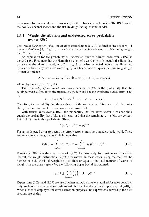
Example 1.4.2 Figure 1.8 shows the values of Pe(C) from (1.33), as a function of the cross-over probability p of a BSC, for the binary repetition (3,1,3) code.

The AWGN channel model

Perhaps the most important channel model in digital communications is the AWGN channel.In this section, expressions are given for the probability of a decoding error and of a biterror for linear block codes over AWGN channels. Although similar expressions hold forconvolutional codes, for clarity of exposition, they are introduced along with the discussionon SDD with the Viterbi algorithm and coded modulation in subsequent chapters. Thefollowing results constitute valuable analysis tools for the error performance evaluation ofbinary coded schemes over AWGN channels.

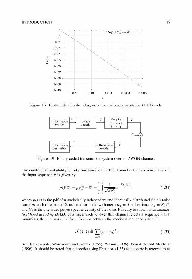
Consider a binary transmission system, with coded bits in the set {0, 1} mapped ontoreal values {+1, −1}, respectively, as illustrated in Figure 1.9. In the following, vectors aren-dimensional and the following notation is used to denote a vector: x = (x0, x1, . . . , xn−1).

INTRODUCTION 17

1e-10

1e-09

1e-08

1e-07

1e-06

1e-05

0.0001

0.001

0.01

0.1

1

1e-050.00010.0010.010.1

Pe(

C)

p

"Pe(3,1,3)_bound"

Figure 1.8 Probability of a decoding error for the binary repetition (3,1,3) code.

01

+1-1

_ _ _

_

_

Binary encoder

Mappingu v x

+

Soft-decisiondecoder

n

yu~

Informationsource

Informationdestination

Figure 1.9 Binary coded transmission system over an AWGN channel.

The conditional probability density function (pdf) of the channel output sequence y, giventhe input sequence x is given by

p(y|x) = pn(y − x) =n−1∏i=0

1√πN0

e− (yi−xi )

2

N0 , (1.34)

where pn(n) is the pdf of n statistically independent and identically distributed (i.i.d.) noisesamples, each of which is Gaussian distributed with mean µn = 0 and variance σn = N0/2,and N0 is the one-sided power spectral density of the noise. It is easy to show that maximum-likelihood decoding (MLD) of a linear code C over this channel selects a sequence x thatminimizes the squared Euclidean distance between the received sequence y and x,

D2(x, y)�=

n−1∑i=0

(xi − yi)2. (1.35)

See, for example, Wozencraft and Jacobs (1965), Wilson (1996), Benedetto and Montorsi(1996). It should be noted that a decoder using Equation (1.35) as a metric is referred to as

18 INTRODUCTION

a soft-decision decoder, independently of whether or not MLD is performed. In Chapter 7,SDD methods are considered.

The probability of a decoding error with MLD, denoted Pe(C), is equal to the probabilitythat a coded sequence x is transmitted and the noise vector n is such that the receivedsequence y = x + n is closer to a different coded sequence x ∈ C, x �= x. For a linear codeC, it can be assumed that the all-zero code word is transmitted. Then Pe(C) can be upperbounded, based on the union bound (Clark and Cain 1981) and the weight distributionW(C), as follows:

Pe(C) ≤n∑

w=dmin

Aw Q

(√2wR

Eb

N0

), (1.36)

where R = k/n is the code rate, Eb/N0 is the energy-per-bit to noise ratio (or SNR perbit) and Q(x) is given by (1.2).

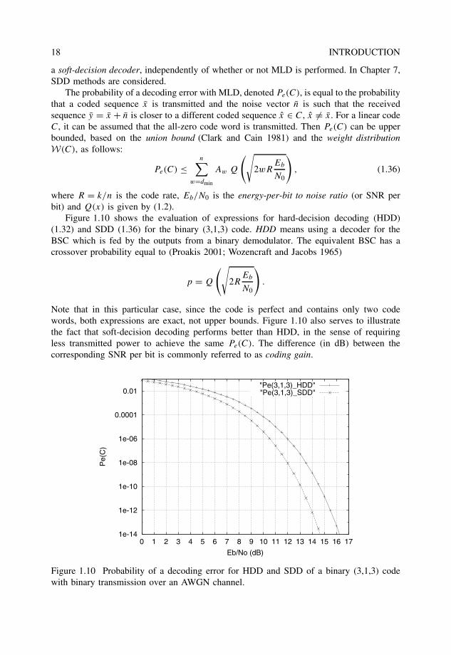
Figure 1.10 shows the evaluation of expressions for hard-decision decoding (HDD)(1.32) and SDD (1.36) for the binary (3,1,3) code. HDD means using a decoder for theBSC which is fed by the outputs from a binary demodulator. The equivalent BSC has acrossover probability equal to (Proakis 2001; Wozencraft and Jacobs 1965)

p = Q

(√2R

Eb

N0

).

Note that in this particular case, since the code is perfect and contains only two codewords, both expressions are exact, not upper bounds. Figure 1.10 also serves to illustratethe fact that soft-decision decoding performs better than HDD, in the sense of requiringless transmitted power to achieve the same Pe(C). The difference (in dB) between thecorresponding SNR per bit is commonly referred to as coding gain.

1e-14

1e-12

1e-10

1e-08

1e-06

0.0001

0.01

0 1 2 3 4 5 6 7 8 9 10 11 12 13 14 15 16 17

Pe(

C)

Eb/No (dB)

"Pe(3,1,3)_HDD""Pe(3,1,3)_SDD"

Figure 1.10 Probability of a decoding error for HDD and SDD of a binary (3,1,3) codewith binary transmission over an AWGN channel.

INTRODUCTION 19

In Fossorier et al. (1998), the authors show that for systematic binary linear codes withbinary transmission over an AWGN channel, the probability of a bit error, denoted Pb(C),has the following upper bound:

Pb(C) ≤n∑

w=dmin

wAw

nQ

(√2wR

Eb

N0

). (1.37)

Interestingly, besides the fact that the above bound holds only for systematic encoding, theresults in Fossorier et al. (1998) show that systematic encoding minimizes the probability ofa bit error. This means that systematic encoding is not only desirable, but actually optimalin the above sense.

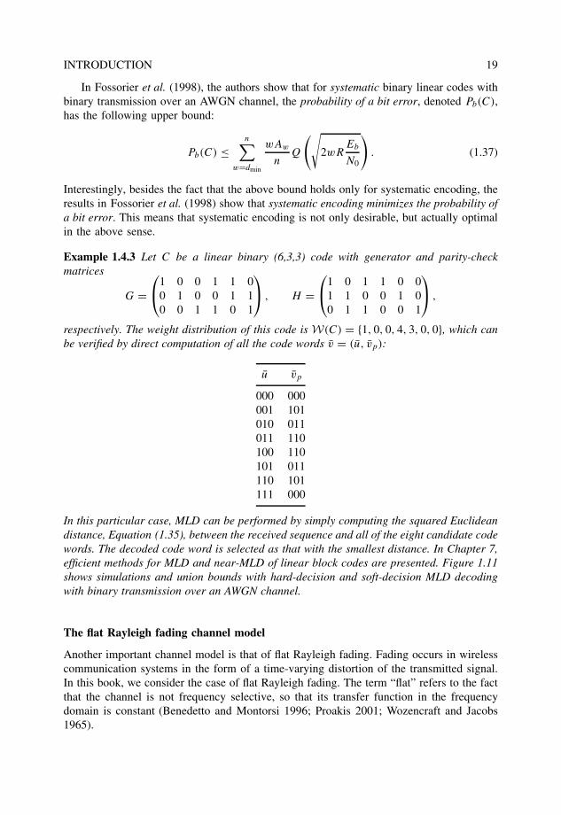
Example 1.4.3 Let C be a linear binary (6,3,3) code with generator and parity-checkmatrices

G =1 0 0 1 1 0

0 1 0 0 1 10 0 1 1 0 1

, H =

1 0 1 1 0 0

1 1 0 0 1 00 1 1 0 0 1

,

respectively. The weight distribution of this code is W(C) = {1, 0, 0, 4, 3, 0, 0}, which canbe verified by direct computation of all the code words v = (u, vp):

u vp

000 000001 101010 011011 110100 110101 011110 101111 000

In this particular case, MLD can be performed by simply computing the squared Euclideandistance, Equation (1.35), between the received sequence and all of the eight candidate codewords. The decoded code word is selected as that with the smallest distance. In Chapter 7,efficient methods for MLD and near-MLD of linear block codes are presented. Figure 1.11shows simulations and union bounds with hard-decision and soft-decision MLD decodingwith binary transmission over an AWGN channel.

The flat Rayleigh fading channel model

Another important channel model is that of flat Rayleigh fading. Fading occurs in wirelesscommunication systems in the form of a time-varying distortion of the transmitted signal.In this book, we consider the case of flat Rayleigh fading. The term “flat” refers to the factthat the channel is not frequency selective, so that its transfer function in the frequencydomain is constant (Benedetto and Montorsi 1996; Proakis 2001; Wozencraft and Jacobs1965).

20 INTRODUCTION

1e-05

0.0001

0.001

0.01

0.1

0 1 2 3 4 5 6 7 8 9 10

Pe(

C)

Eb/No (dB)

"Pe(6,3,3)_HDB""Pe(6,3,3)_HDD"

"Pe(6,3,3)_UB""Pe(6,3,3)_SDD"

Figure 1.11 Simulations and union bounds for the binary (6,3,3) code. Binary transmissionover an AWGN channel.

01

+1-1

___

_

_

_

Binary encoder

Mappingu v x

Soft-decisiondecoder

yu~

Informationsource

Informationdestinatio n

n

a

+

x

Figure 1.12 Binary coded transmission system over a flat Rayleigh fading channel.

As a result, a (component-wise) multiplicative distortion is present in the channel, asshown in the model depicted in Figure 1.12, where α is a vector with n component i.i.d.random variables αi , 0 ≤ i < n, each having a Rayleigh pdf,

pαi(αi) = αi e−α2

i/2, αi ≥ 0. (1.38)

With this pdf, the average SNR per bit equals Eb/N0 (i.e., that of the AWGN), since thesecond moment of the fading amplitudes is E{α2

i } = 1.In evaluating the performance of a binary linear code over a flat Rayleigh fading chan-

nel, a conditional probability of a decoding error, Pe(C|α), or of a bit error, Pb(C|α), iscomputed. The unconditional error probabilities are then obtained by integration over aproduct of αi , with pdf given by Equation (1.38).

The conditional probabilities of error are identical to those obtained for binary transmis-sion over an AWGN channel. The main difference is that the arguments in the Q(x) function,which correspond to the pairwise probability of a decoding error, are now weighted by thefading amplitudes αi . Considering a coded binary transmission system without channel

INTRODUCTION 21

state information (CSI), we have that

Pe(C|α) ≤n∑

w=dmin

Aw Q

(√1

w�2

w2REb

N0

), (1.39)

with

�w =w∑

i=1

αi. (1.40)

Finally, the probability of a decoding error with binary transmission over a flat Rayleighfading channel is obtained by taking the expectation with respect to �w ,

Pe(C) ≤n∑

w=dmin

Aw

∫ ∞

0Q

(√1

w�2

w2REb

N0

)p�w(�w)d�w. (1.41)

There are several methods to evaluate or further upper bound expression (1.41). One is toevaluate numerically (1.41) by Monte Carlo (MC) integration, with the approximation

Pe(C)<∼ 1

N

N∑�=1

n∑w=dmin

Aw Q

(√2�w(�)R

Eb

N0

), (1.42)

where �w(�) denotes the sum of the squares of w i.i.d. random variables with Rayleighdistribution, given by (1.40), generated in the �-th outcome of a computer program, andN is a sufficiently large number that depends on the range of values of Pe(C). A goodrule of thumb is that N should be at least 100 times larger than the inverse of Pe(C).(See Jeruchim et al. (1992), pp. 500–503.)

Another method is to bound the Q-function by an exponential function (see, e.g.,(Wozencraft and Jacobs 1965), pp. 82–84) and to perform the integration, or to find aChernoff bound. This approach results in a loose bound that, however, yields a closedexpression (see also Wilson (1996), p. 526, and Benedetto and Montorsi (1996), p. 718):

Pe(C) ≤n∑

w=dmin

Aw

1(1 + REb

N0

)w . (1.43)

The bound (1.43) is useful in cases where a first-order estimation of the code performanceis desired.

Example 1.4.4 Figure 1.13 shows computer simulation results SIM of the binary (3,1,3)code over a flat Rayleigh fading channel. Note that the MC integration of the union boundgives exactly the actual error performance of the code, since there is only one term in thebound. Also note that the Chernoff bound is about 2 dB away from the simulations, at anSNR per bit En/N0 > 18 dB.

Example 1.4.5 Figure 1.14 shows the results of computer simulations of decoding the binary(6,3,3) code of Example 1.4.3, over a flat Rayleigh fading channel. In this case, the unionbound is relatively loose at low values of Eb/N0 due to the presence of more terms in thebound. Again, it can be seen that the Chernoff bound is loose by about 2 dB, at an SNR perbit En/N0 > 18 dB.

22 INTRODUCTION

1e-05

0.0001

0.001

0.01

0.1

5 6 7 8 9 10 11 12 13 14 15 16 17 18 19 20

Pe(

C)

Eb/No (dB)

"Pe(3,1,3)_MC""Pe(3,1,3)_EXP"

"SIM"

Figure 1.13 Simulation results (SIM), compared with the Monte Carlo union bound(Pe(3,1,3) MC) and the Chernoff bound (Pe(3,1,3) EXP), for the binary (3,1,3) code. Binarytransmission over a flat Rayleigh fading channel.

1e-05

0.0001

0.001

0.01

0.1

5 6 7 8 9 10 11 12 13 14 15 16 17 18 19 20

Pe(

C)

Eb/No (dB)

"SIM_(6,3,3)""Pe(6,3,3)_MC"

"Pe(6,3,3)_EXP"

Figure 1.14 Simulation results (SIM (6,3,3)), compared with the Monte Carlo union bound(Pe(6,3,3) MC) and the Chernoff bound (Pe(6,3,3) EXP), for the binary (6,3,3) code. Binarytransmission over a flat Rayleigh fading channel.

INTRODUCTION 23

Buffer received vector +

_

___Compute

syndromeFind error

vectorr s e

v ’

Figure 1.15 General structure of a hard-decision decoder of a linear block code for theBSC model.

1.5 General structure of a hard-decision decoderof linear codes

In this section, the general structure of a hard-decision decoder for linear codes is summa-rized. Figure 1.15 shows a simple block diagram of the decoding process. Note that sincehard decisions are assumed, bits at the output of a demodulator are fed into a decoderdesigned for a BSC.

Let v ∈ C denote a transmitted code word. The decoder has at its input a noisy receivedvector r = v + e. A two-step decoding procedure of a linear code is:

• Compute the syndrome s = rH�. On the basis of the code properties, the syndromeis a linear transformation of the error vector introduced in the channel,

s = eH�, (1.44)

• On the basis of the syndrome s, estimate the most likely error vector e and subtractit (modulo 2 addition in the binary case) from the received vector.

Although most practical decoders will not perform the above procedure as stated, it isnonetheless instructive to think of a hard-decision decoder as implementing a methodof solving equation (1.44). Note that any method of solving this equation constitutes adecoding method. For example, one could attempt to solve the key equation by finding apseudoinverse of H�, denoted (H�)+, such that H�(H�)+ = In, and the solution

e = s(H�)+, (1.45)

has the smallest Hamming weight possible. As easy as this may sound, it is a formidabletask. This issue will be visited again when discussing decoding methods for Bose-Chauduri-Hocquenghem (BCH) and Reed-Solomon (RS) codes.

Problems

1. Write a computer program to simulate a binary communication system with binaryphase shift keying (BPSK) modulation over an AWGN channel. (Hint: Generate ran-dom values S ∈ {−1, +1} so that Eb = 1. To generate a sample W of AWGN, first

24 INTRODUCTION

generate a Gaussian random variable N of zero mean and unit variance. The transfor-mation W = σW N then results in a Gaussian random variable W of zero mean andvariance σ 2

W = N0/2. Given a value of Eb/N0 in dB, compute N0 =√

10(−(Eb/No)/10).The receiver estimates (RE) the value S based on the sign of the received valueR = S + W . An error event occurs whenever S �= S.)

2. Prove that in general a total of 2k−1(2k − 1) code word pairs need to be examinedin a block code to determine its minimum distance.

3. Prove that GsysHTsys = 0k,n−k.

4. Prove the nonbinary version of the Hamming bound, that is, inequality (1.27).

5. A binary linear block code C has a generator matrix

G =(

1 0 11 1 0

)

(a) Find the weight distribution W(C).

(b) Using elementary matrix operations, bring G into a systematic form G′ thatgenerates a binary linear block code C ′.

(c) Using the weight distribution W(C ′), argue that G and G′ generate the samelinear code, up to a permutation in bit positions.

6. A binary linear block code C has a generator matrix

G =1 0 0 1 1

0 1 0 1 00 0 1 0 1

(a) What are the values of length n and dimension k of this code?

(b) Find the weight distribution W(C) and use it to determine the probability of anundetected error.

(c) Determine the error correcting capability t of C.

(d) Find a parity-check matrix H of C.

(e) Find the standard array of C, based on H of part (c).

(f) Use standard array decoding to find the closest code word to the received wordr = (11011).

7. Carefully sketch circuits used in encoding and decoding of a binary linear (5,3,2)code with generator matrix

G =1 0 0 1 1

0 1 0 1 00 0 1 0 1

INTRODUCTION 25

8. Prove that the decoding region Colj centered around a code word vj ∈ C of a linearcode C contains the Hamming sphere St (vj ), that is,

St (vj ) ⊆ Colj

9. Use the Hamming bound to disprove the existence of a binary linear (32, 24, 5) code.

10. A network designer needs to correct up to 3 random errors in 64 information bits.What is the minimum amount of redundant bits required?

11. A memory system uses a bus with 64 information bits and 16 redundant bits. Withparallel processing (80 bits at a time), what is that maximum number of errors thatcan be corrected?

12. Determine the smallest length of a binary linear code capable of correcting any tworandom bit errors in 21 information bits.

13. Let C be a binary linear (5, 2, dmin) code.

(a) With the aid of the Hamming bound, determine the minimum Hamming distancedmin of C.

(b) Find a generator matrix and a parity-check matrix of C.

(c) Determine the exact probability of a decoding error Pe(C) over a BSC withcrossover probability p.

14. Using the union bound on the error performance of a linear block code with binarytransmission over an AWGN channel, show that the binary (3, 1, 3) repetition codeoffers no advantage over uncoded BPSK modulation. Generalize the result to allbinary (n, 1, n) repetition codes and comment on the basic trade-off involved.

15. Show that the binary (3, 1, 3) repetition code C outperforms BPSK modulation withtransmission over a flat Rayleigh fading channel. Specifically, show that the slope ofthe bit-error-rate (BER) curve of C is three times more negative than that of uncodedbinary phase shift keying (BPSK) modulation. (Thus, C has a diversity order equalto three.)

16. Compare the probability of a bit error, with binary modulation over an AWGN chan-nel, of a binary (3, 1, 3) repetition code and the binary linear (4, 2, 2) code introducedin Example 1.3.1. What is the difference in performance measured in dB?

17. Compare the performance of the two codes in the previous problem with binarytransmission over a Rayleigh fading channel.

18. (Peterson and Weldon (1972)) Given a binary linear (n1, k, d1) code and a binary lin-ear (n2, k, d2) code, construct a binary linear (n1 + n2, k, d) code with d ≥ d1 + d2.