introduction - cs.le.ac.uk

BITOPOLOGICAL DUALITY FOR DISTRIBUTIVE LATTICES AND

HEYTING ALGEBRAS

GURAM BEZHANISHVILI, NICK BEZHANISHVILI, DAVID GABELAIA, ALEXANDER KURZ

Abstract. We introduce pairwise Stone spaces as a natural bitopological generalization ofStone spaces—the duals of Boolean algebras—and show that they are exactly the bitopolog-ical duals of bounded distributive lattices. The category PStone of pairwise Stone spacesis isomorphic to the category Spec of spectral spaces and to the category Pries of Priestleyspaces. In fact, the isomorphism of Spec and Pries is most naturally seen through PStone

by first establishing that Pries is isomorphic to PStone, and then showing that PStone isisomorphic to Spec. We provide the bitopological and spectral descriptions of many alge-braic concepts important for the study of distributive lattices. We also give new bitopologicaland spectral dualities for Heyting algebras, co-Heyting algebras, and bi-Heyting algebras,thus providing two new alternatives of Esakia’s duality.

1. Introduction

It is widely considered that the beginning of duality theory was Stone’s groundbreakingwork in the mid 30ies on the dual equivalence of the category Bool of Boolean algebrasand Boolean algebra homomorphism and the category Stone of compact Hausdorff zero-dimensional spaces, which became known as Stone spaces, and continuous functions. In 1937Stone [28] extended this to the dual equivalence of the category DLat of bounded distributivelattices and bounded lattice homomorphisms and the category Spec of what later becameknown as spectral spaces and spectral maps. Spectral spaces provide a generalization of Stonespaces. Unlike Stone spaces, spectral spaces are not Hausdorff (not even T1)

1, and as a result,are more difficult to work with. In 1970 Priestley [20] described another dual category ofDLat by means of special ordered Stone spaces, which became known as Priestley spaces,thus establishing that DLat is also dually equivalent to the category Pries of Priestley spacesand continuous order-preserving maps. Since DLat is dually equivalent to both Spec andPries, it follows that the categories Spec and Pries are equivalent. In fact, more is true:as shown by Cornish [4] (see also Fleisher [8]), Spec is actually isomorphic to Pries. Theadvantage of Priestley spaces is that they are easier to work with than spectral spaces. As aresult, Priestley’s duality became rather popular, and most dualities for distributive latticeswith operators have been performed in terms of Priestley spaces. Here we only mentionEsakia’s duality for Heyting algebras, co-Heyting algebras, and bi-Heyting algebras [5, 6],which is a restricted version of Priestley’s duality.2 On the other hand, the advantage ofspectral spaces is that they only have a topological structure, while Priestley spaces also

2000 Mathematics Subject Classification. 06D50; 06D20; 54E55.Key words and phrases. Distributive lattices, Heyting algebras, duality theory, bitopologies.1In fact, a spectral space X is a Stone space iff X is T1.2We note that Esakia’s work was independent of Priestley’s; a proof that Esakia spaces are Priestley

spaces can be found in [7, p. 62].1

2 GURAM BEZHANISHVILI, NICK BEZHANISHVILI, DAVID GABELAIA, ALEXANDER KURZ

have an order structure on top of topology, thus their signature is more complicated thanthat of spectral spaces.

Another way to represent distributive lattices is by means of bitopological spaces, asdemonstrated by Jung and Moshier [15]. In fact, bitopological spaces provide a naturalmedium in establishing the isomorphism between Pries and Spec: with each Priestley space(X, τ,≤), there are two natural topologies associated with it; the upper topology τ1 consistingof open upsets of (X, τ,≤), and the lower topology τ2 consisting of open downsets of (X, τ,≤).Then (X, τ1, τ2) is a bitopological space, and the spectral space associated with (X, τ,≤) isobtained from (X, τ1, τ2) by forgetting τ2. In this paper we provide an explicit axiomatizationof the class of bitopological spaces obtained this way. We call these spaces pairwise Stonespaces. On the one hand, pairwise Stone spaces provide a natural generalization of Stonespaces as each of the three conditions defining a Stone space naturally generalizes to thebitopological setting: compact becomes pairwise compact, Hausdorff – pairwise Hausdorff,and zero-dimensional – pairwise zero-dimensional. On the other hand, pairwise Stone spacesprovide a natural medium in moving from Priestley spaces to spectral spaces and backwards,thus Cornish’s isomorphism of Pries and Spec can be established more naturally by firstshowing that Pries is isomorphic to the category PStone of pairwise Stone spaces andbicontinuous maps, and then showing that PStone is isomorphic to Spec. Thirdly, thesignature of pairwise Stone spaces naturally carries the symmetry present in Priestley spaces(and distributive lattices), but hidden in spectral spaces. Moreover, the proof that DLat isdually equivalent to PStone is simpler and more natural than the existing proofs of the dualequivalence of DLat with Spec and Pries. Lastly, the isomorphism of Pries, PStone, andSpec fits nicely in a more general isomorphism of the categories of compact order-Hausdorffspaces, pairwise compact pairwise regular bitopological spaces, and stably compact spacesdescribed in [10, Ch. VI-6] (see also [25] and [19]). For a variety of applications of theseresults we refer to the work of Jung, Moshier, and their collaborators [13, 14, 2, 15]. Here weonly mention that there is a dual equivalence between these categories and the category ofproximity lattices [27, 16], which are a generalization of distributive lattices, thus providingan interesting generalization of the duality for distributive lattices. We view our pairwiseStone spaces as a particular case of pairwise compact pairwise regular bitopological spaces,and our isomorphism of the categories of Priestley spaces, pairwise Stone spaces, and spectralspaces as a particular case of the isomorphism of the categories of compact order-Hausdorffspaces, pairwise compact pairwise regular bitopological spaces, and stably compact spaces.

One of the advantages of Priestley’s duality is that many algebraic concepts importantfor the study of distributive lattices can be easily described by means of Priestley spaces.In addition, we show that they have a natural dual description by means of pairwise Stonespaces. We also give their dual description by means of spectral spaces, which at times is lesstransparent than the order topological and bitopological descriptions. We conclude the paperby introducing the subcategories of PStone and Spec, which are isomorphic to the categoryEsa of Esakia spaces and dually equivalent to the category Heyt of Heyting algebras. Thisprovides an alternative of Esakia’s duality in the setting of bitopological spaces and spectralspaces. In addition, we establish similar dual equivalences for the categories of co-Heytingalgebras and bi-Heyting algebras.

The paper is organized as follows. In Section 2 we recall some basic facts about bitopo-logical spaces, introduce pairwise Stone spaces, and study their basic properties. In Section3 we prove that the category PStone of pairwise Stone spaces is isomorphic to the category

BITOPOLOGICAL DUALITY FOR DISTRIBUTIVE LATTICES AND HEYTING ALGEBRAS 3

Pries of Priestley spaces. In Section 4 we prove that PStone is isomorphic to the categorySpec of spectral spaces, thus establishing that all three categories are isomorphic to eachother. In Section 5 we give a direct proof that the category DLat of distributive latticesis dually equivalent to PStone, thus providing an alternative of Stone’s and Priestley’s du-alities. In Section 6 we give the dual description of many algebraic concepts important forthe study of distributive lattices by means of Priestley spaces, pairwise Stone spaces, andspectral spaces. In particular, we give the dual description of filters, prime filters, maximalfilters, ideals, prime ideals, maximal ideals, homomorphic images, sublattices, complete lat-tices, McNeille completions, and canonical completions. At the end of the section we listall the obtained results in one table, which can be viewed as a dictionary of duality theoryfor distributive lattices, complementing the dictionary given in [22]. Finally, in Section 7 wedevelop new bitopological and spectral dualities for Heyting algebras, co-Heyting algebras,and bi-Heyting algebras, thus providing an alternative of Esakia’s duality.

2. Pairwise Stone spaces

We recall that a bitopological space is a triple (X, τ1, τ2), where X is a nonempty set andτ1 and τ2 are two topologies on X. Ever since Kelly [17] introduced them, bitopologicalspaces have been subject of intensive investigation of many topologists. In particular, therehas been a lot of research on the “correct” generalization of the basic topological propertiesto the bitopological setting. For our purposes it is important to find the right generalizationof the concept of a Stone space. Therefore, we are interested in the bitopological versions ofcompactness, Hausdorffness, and zero-dimensionality.

There are several ways to generalize a topological property to the bitopological setting.Let (X, τ1, τ2) be a bitopological space and let τ = τ1 ∨ τ2. For a topological property P , wesay that (X, τ1, τ2) is bi-P if both (X, τ1) and (X, τ2) are P , and we say that (X, τ1, τ2) is joinP if (X, τ) is P . For example, (X, τ1, τ2) is bi-T0, bi-T1, or bi-T2 if both (X, τ1) and (X, τ2)are T0, T1, or T2, respectively; and (X, τ1, τ2) is join T0, join T1, or join T2 if (X, τ) is T0, T1,or T2, respectively. However, for our purposes, neither bi-Stone nor join Stone turns out tobe the right generalization of the concept of a Stone space to the bitopological setting.

Definition 2.1. Let (X, τ1, τ2) be a bitopological space.

(1) [24, Def. 2.1.1] We call (X, τ1, τ2) pairwise T0 if for any two distinct points x, y ∈ Xthere exists U ∈ τ1 ∪ τ2 containing exactly one of x, y.

(2) [24, Def. 2.1.3] We call (X, τ1, τ2) pairwise T1 if for any two distinct points x, y ∈ Xthere exists U ∈ τ1 ∪ τ2 such that x ∈ U and y /∈ U .

(3) [24, Def. 2.1.8] We call (X, τ1, τ2) pairwise T2 or pairwise Hausdorff if for any twodistinct points x, y ∈ X there exist disjoint U ∈ τ1 and V ∈ τ2 such that x ∈ U andy ∈ V or there exist disjoint U ∈ τ2 and V ∈ τ1 with the same property.

Remark 2.2. We have chosen [24] as our primary source of reference, although the conceptsof a pairwise T0 space and a pairwise T1 space have appeared earlier in the literature.

Remark 2.3. It would be more in the vein of Definition 2.1.1 and 2.1.2 if we defined apairwise T2 space as a bitopological space satisfying the following condition: For any twodistinct points x, y ∈ X there exist disjoint U, V ∈ τ1 ∪ τ2 such that x ∈ U and y ∈ V .Obviously if (X, τ1, τ2) is pairwise T2, then it satisfies the condition above, but the converseis not true in general. Nevertheless, we will show below that in the realm of pairwise zero-dimensional spaces the two conditions are equivalent.


It follows from [24, Prop. 2.1.2 and 2.1.5] that each pairwise Ti space is join Ti for i = 0, 1.However, not every pairwise T2 space is join T2. It is also obvious that bi-Ti implies pairwiseTi for i = 0, 1, 2, but there are pairwise T2 spaces that are not even bi-T0. As we will seeshortly, the concepts of bi-T0, pairwise T2, and join T2 coincide in the realm of pairwisezero-dimensional spaces.

For a bitopological space (X, τ1, τ2), let δ1 denote the collection of closed subsets of (X, τ1)and δ2 denote the collection of closed subsets of (X, τ2). The next definition generalizes thenotion of zero-dimensionality to bitopological spaces.

Definition 2.4. [23, p. 127] We call a bitopological space (X, τ1, τ2) pairwise zero-dimensionalif opens in (X, τ1) closed in (X, τ2) form a basis for (X, τ1) and opens in (X, τ2) closed in(X, τ1) form a basis for (X, τ2); that is, β1 = τ1 ∩ δ2 is a basis for τ1 and β2 = τ2 ∩ δ1 is abasis for τ2.

We point out that if (X, τ1, τ2) is pairwise zero-dimensional, then β2 = {U c | U ∈ β1} andβ1 = {V c | V ∈ β2}. Moreover, both β1 and β2 contain ∅, X and are closed with respect tofinite unions and intersections.

Lemma 2.5. Suppose that (X, τ1, τ2) is pairwise zero-dimensional. Then the following con-ditions are equivalent:

(1) (X, τ1) is T0.(2) (X, τ2) is T0.(3) (X, τ1, τ2) is pairwise T2.(4) For any two distinct points x, y ∈ X there exist disjoint U, V ∈ τ1 ∪ τ2 such that

x ∈ U and y ∈ V .(5) (X, τ1, τ2) is join T2.(6) (X, τ1, τ2) is bi-T0.

Proof. (1)⇒(2): Suppose that (X, τ1) is T0 and x, y are two distinct points of X. Thenthere exists U ∈ τ1 containing exactly one of x, y. Without loss of generality we may assumethat x ∈ U and y /∈ U . Since (X, τ1, τ2) is pairwise zero-dimensional, there exists V ∈ β1

such that x ∈ V ⊆ U . Therefore, V c ∈ β2, y ∈ Vc, and x /∈ V c. Thus, (X, τ2) is T0.

(2)⇒(3): Suppose that (X, τ2) is T0 and x, y are two distinct points of X. Then thereexists U ∈ τ2 containing exactly one of x, y. Without loss of generality we may assume thatx ∈ U and y /∈ U . Since (X, τ1, τ2) is pairwise zero-dimensional, there exists V ∈ β2 suchthat x ∈ V ⊆ U . Then x ∈ V ∈ β2, y ∈ V

c ∈ β1, and V, V c are disjoint. Thus, (X, τ1, τ2) ispairwise T2.

(3)⇒(4) is obvious.(4)⇒(5): Suppose that x, y are two distinct points of X. By (4), there exist disjoint

U, V ∈ τ1 ∪ τ2 such that x ∈ U and y ∈ V . Without loss of generality we may assumethat U, V ∈ τ1. Since (X, τ1, τ2) is pairwise zero-dimensional, there exists U ′ ∈ β1 such thatx ∈ U ′ ⊆ U . Let V ′ = X −U ′. Then V ⊆ V ′, so y ∈ V ′ ∈ β2, and so there exist two disjointτ -open sets U ′, V ′ such that x ∈ U ′ and y ∈ V ′. Thus, (X, τ1, τ2) is join T2.

(5)⇒(6): Suppose that (X, τ1, τ2) is join T2. We show that (X, τ1) is T0. Let x, y be twodistinct points of X. Since (X, τ1, τ2) is pairwise zero-dimensional and join T2, there existU1, U2 ∈ β1 and V1, V2 ∈ β2 such that x ∈ U1 ∩ V1, y ∈ U2 ∩ V2, and U1 ∩ V1 and U2 ∩ V2

are disjoint. If y /∈ U1, then there is U1 ∈ τ1 containing exactly one of x, y. If y ∈ U1, theny /∈ V1. Therefore, y ∈ U2 ∩ V

c1 . Clearly U2 ∩ V

c1 ∈ β1. Moreover, x /∈ U2 ∩ V

c1 as x /∈ V c

1 .Thus, there exists U2∩V

c1 ∈ τ1 containing exactly one of x, y. In either case, we separate x, y


by a τ1-open set, and so (X, τ1) is T0. That (X, τ2) is T0 is proved similarly. Consequently,(X, τ1, τ2) is bi-T0.

(6)⇒(1) is obvious. ⊣

On the other hand, (X, τ1, τ2) may be pairwise zero-dimensional and pairwise T2 withouteither of τ1, τ2 being even T1 as the following simple example shows.

Example 2.6. Let X = {0, 1}, τ1 = {∅, {1}, X} and τ2 = {∅, {0}, X}. Then both τ1 and τ2are the Sierpinski topologies on X, thus both are T0, but not T1. Nevertheless, (X, τ1, τ2) ispairwise zero-dimensional and pairwise T2.

The next definition generalizes the notion of compactness to bitopological spaces.

Definition 2.7. [24, Def. 2.2.17] We call a bitopological space (X, τ1, τ2) pairwise compactif for each cover {Ui | i ∈ I} of X with Ui ∈ τ1 ∪ τ2, there exists a finite subcover.

Remark 2.8. In [24, Def. 2.2.17] Salbany defines a bitopological space (X, τ1, τ2) to bepairwise compact if (X, τ) is compact, where τ = τ1∨τ2. In our terminology this means that(X, τ1, τ2) is join compact. But it is a consequence of Alexander’s Lemma—a classical resultin general topology—that the two notions of pairwise compact and join compact coincide.

It is obvious that if (X, τ1, τ2) is pairwise compact, then both (X, τ1) and (X, τ2) arecompact; that is, (X, τ1, τ2) is bi-compact. On the other hand, it was observed by Salbany[24, p. 17] that the converse is not true in general. Let σ1 and σ2 denote the collections ofcompact subsets of (X, τ1) and (X, τ2), respectively.

Proposition 2.9. A bitopological space (X, τ1, τ2) is pairwise compact iff δ1 ⊆ σ2 and δ2 ⊆σ1.

Proof. [⇒] Suppose that (X, τ1, τ2) is pairwise compact. We show that δ1 ⊆ σ2. Let A ∈ δ1and let A ⊆

⋃{Ui | i ∈ I} with {Ui | i ∈ I} ⊆ τ2. Then the collection {Ui | i ∈ I} ∪ {A

c}is a cover of X. Since Ac ∈ τ1 and (X, τ1, τ2) is pairwise compact, there exist i1, . . . , in ∈ Isuch that Ui1 ∪ · · · ∪Uin ∪A

c = X. It follows that A ⊆ Ui1 ∪ · · · ∪Uin , and so A ∈ σ2. Thus,δ1 ⊆ σ2. That δ2 ⊆ σ1 is proved similarly.

[⇐] Suppose that δ1 ⊆ σ2 and δ2 ⊆ σ1. To show that (X, τ1, τ2) is pairwise compact let{Ui | i ∈ I} ⊆ τ1 and {Vj | j ∈ J} ⊆ τ2 with

⋃{Ui | i ∈ I} ∪

⋃{Vj | j ∈ J} = X. We set

U =⋃{Ui | i ∈ I}. Clearly U ∈ τ1 and U∪

⋃{Vj | j ∈ J} = X, so U c ⊆

⋃{Vj | j ∈ J}. Since

U c ∈ δ1 and δ1 ⊆ σ2, we have that U c ∈ σ2. Therefore, there exist j1, . . . , jn ∈ J such thatU c ⊆ Vj1∪· · ·∪Vjn

. We set V = Vj1∪· · ·∪Vjn. Then U∪V = X, so V c ⊆ U =

⋃{Ui | i ∈ I}.

Since V c ∈ δ2 and δ2 ⊆ σ1, we have that V c ∈ σ1. Therefore, there exist i1, . . . , im ∈ I suchthat V c ⊆ Ui1 ∪ · · · ∪ Uim . Clearly the finite collection {Vj1, . . . , Vjn

, Ui1 , . . . , Uim} is a coverof X. Thus, X is pairwise compact. ⊣

Now we generalize the notion of a Stone space to that of a pairwise Stone space.

Definition 2.10. We call (X, τ1, τ2) a pairwise Stone space if it is pairwise compact, pairwiseHausdorff, and pairwise zero-dimensional.

We note that in the definition of a pairwise Stone space, pairwise Hausdorff can be replacedby any of the equivalent conditions of Lemma 2.5, and that pairwise compact can be replacedby δ1 ⊆ σ2 and δ2 ⊆ σ1, as follows from Proposition 2.9. Let PStone denote the categoryof pairwise Stone spaces and bi-continuous functions; that is functions which are continuouswith respect to both topologies.


3. Priestley spaces and pairwise Stone spaces

Let (X,≤) be a poset. We recall that A ⊆ X is an upset if x ∈ A and x ≤ y implyy ∈ A, and that A is a downset if x ∈ A and y ≤ x imply y ∈ A. For Y ⊆ X let↑Y = {x | ∃y ∈ Y with y ≤ x} and ↓Y = {x | ∃y ∈ Y with x ≤ y}. Let Up(X) denote theset of upsets and Do(X) denote the set of downsets of (X,≤).

Let (X, τ,≤) be an ordered topological space. We denote by OpUp(X) the set of openupsets, by ClUp(X) the set of closed upsets, and by CpUp(X) the set of clopen upsets of(X, τ,≤). Similarly, let OpDo(X) denote the set of open downsets, ClDo(X) denote the setof closed downsets, and CpDo(X) denote the set of clopen downsets of (X, τ,≤). The nextdefinition is well-known.

Definition 3.1. An ordered topological space (X, τ,≤) is a Priestley space if (X, τ) is com-pact and whenever x 6≤ y, there exists a clopen upset A such that x ∈ A and y 6∈ A.

The second condition in the above definition is known as the Priestley separation axiom(PSA for short). The next lemma is well-known.

Lemma 3.2. Let (X, τ,≤) be an ordered topological space.

(1) If (X, τ,≤) is a Priestley space, then (X, τ) is a Stone space.(2) If (X, τ,≤) is a Priestley space, then ↑F and ↓F are closed for each closed subset F

of X.(3) In a Priestley space, every open upset is the union of clopen upsets, every closed

upset is the intersection of clopen upsets, every open downset is the union of clopendownsets, and every closed downset is the intersection of clopen downsets.

(4) In a Priestley space, clopen upsets and clopen downsets form a subbasis for the topol-ogy.

(5) (X, τ,≤) is a Priestley space iff (X, τ) is compact and for closed subsets F and G ofX, whenever ↑F ∩ ↓G = ∅, there exists a clopen upset A of X such that F ⊆ A andG ⊆ Ac.

We will refer to condition (5) in the lemma as the strong Priestley separation axiom (SPSAfor short). Let Pries denote the category of Priestley spaces and continuous order-preservingmaps. We show that the categories Pries and PStone are isomorphic. To this end, we willdefine two functors Φ : PStone → Pries and Ψ : Pries → PStone which will set therequired isomorphism.

For a topological space (X, τ), let ≤ denote the specialization order of (X, τ); that is,

x ≤ y iff x ∈ Cl(y) iff (∀U ∈ τ)(x ∈ U implies y ∈ U).

It is well-known that ≤ is reflexive and transitive, and that ≤ is antisymmetric iff (X, τ) isT0.

Lemma 3.3. Let (X, τ1, τ2) be a bitopological space, ≤1 be the specialization order of (X, τ1),and ≤2 be the specialization order of (X, τ2). If (X, τ1, τ2) is pairwise zero-dimensional, then≤1=≥2.

Proof. Let (X, τ1, τ2) be pairwise zero-dimensional; that is, β1 = τ1 ∩ δ2 is a basis for τ1and β2 = τ2 ∩ δ1 is a basis for τ2. Then, for each x, y ∈ X, we have:


x ≤1 y iff(∀U ∈ τ1)(x ∈ U implies y ∈ U) iff(∀U ∈ β1)(x ∈ U implies y ∈ U) iff(∀U ∈ β1)(y ∈ U

c implies x ∈ U c) iff(∀V ∈ β2)(y ∈ V implies x ∈ V ) iff(∀V ∈ τ2)(y ∈ V implies x ∈ V ) iffy ≤2 x.

⊣

For a pairwise Stone space (X, τ1, τ2), let τ = τ1 ∨ τ2, and let ≤=≤1 be the specializationorder of (X, τ1).

Proposition 3.4. If (X, τ1, τ2) is a pairwise Stone space, then (X, τ,≤) is a Priestley space.Moreover:

(i) CpUp(X, τ,≤) = β1.(ii) OpUp(X, τ,≤) = τ1.(iii) ClUp(X, τ,≤) = δ2.(iv) CpDo(X, τ,≤) = β2.(v) OpDo(X, τ,≤) = τ2.(vi) ClDo(X, τ,≤) = δ1.

Proof. Since (X, τ1, τ2) is pairwise compact, (X, τ1, τ2) is join compact, and so (X, τ) iscompact. Also, as (X, τ1, τ2) is pairwise Hausdorff, it follows from Lemma 2.5 that (X, τ1) isT0. Therefore, ≤=≤1 is a partial order. We show that (X, τ,≤) satisfies PSA. If x 6≤ y, thenx 6≤1 y, so there exists U ∈ β1 such that x ∈ U and y 6∈ U . Since ≤1 is the specializationorder of (X, τ1), U is an ≤1-upset. From U ∈ β1 it follows that U c ∈ β2 ⊆ τ . So both Uand U c are open in (X, τ), and so U is clopen in (X, τ). Therefore, U is a clopen upset of(X, τ,≤), implying that (X, τ,≤) satisfies PSA. Thus, (X, τ,≤) is a Priestley space.

(i) We already showed that β1 ⊆ CpUp(X, τ,≤). Let A ∈ CpUp(X, τ,≤). We show thatA =

⋃{U ∈ β1 | U ⊆ A}. That

⋃{U ∈ β1 | U ⊆ A} ⊆ A is obvious. Let x ∈ A. Since A is

an upset, for each y ∈ Ac we have x 6≤ y. Therefore, x 6≤1 y, and as β1 is a basis for (X, τ1),there exists Uy ∈ β1 such that x ∈ Uy and y 6∈ Uy. It follows that Ac ∩

⋂{Uy | y ∈ A

c} = ∅.Thus, {Ac}∪{Uy | y ∈ A

c} is a family of closed subsets of (X, τ) with the empty intersection,and as (X, τ) is compact, there are U1, . . . , Un ∈ β1 with Ac ∩ U1 ∩ · · · ∩ Un = ∅. Therefore,x ∈ U1 ∩ · · · ∩ Un ⊆ A. Since β1 is closed under finite intersections, we obtain that there isU ∈ β1 such that x ∈ U ⊆ A. Thus, A =

⋃{U ∈ β1 | U ⊆ A}. Now since A is a closed

subset of a compact space, A is compact, so it is a finite union of elements of β1, thus A ∈ β1.(ii) Since every open upset is the union of clopen upsets of (X, τ,≤) and β1 is a basis for

(X, τ1), the result follows from (i).(iv) and (v) are proved similar to (i) and (ii).(iii) Since closed upsets are intersections of clopen upsets of (X, τ,≤), and clopen upsets are

elements of β1, closed upsets are intersections of elements of β1. Because β1 = {U c | U ∈ β2},intersections of elements of β1 are intersections of complements of elements of β2, so arecomplements of unions of elements of β2. As unions of elements of β2 are elements ofτ2, we obtain that closed upsets are complements of elements of τ2, so are elements of δ2.Consequently, ClUp(X, τ,≤) = δ2.

(vi) is proved similar to (iii). ⊣


Proposition 3.5. Let (X, τ1, τ2) and (X ′, τ ′1, τ′

2) be pairwise Stone spaces. If f : (X, τ1, τ2)→(X ′, τ ′1, τ

′

2) is bi-continuous, then f : (X, τ,≤) → (X ′, τ ′,≤′) is continuous and order-preserving.

Proof. Since f is bi-continuous, the f inverse image of every element of τ ′1 ∪ τ′

2 is anelement of τ1 ∪ τ2. As τ ′1 ∪ τ

′

2 is a subbasis for (X, τ ′), it follows that f : (X, τ)→ (X ′, τ ′) iscontinuous. Also, since the f inverse image of an element of τ ′1 is an element of τ1 and ≤′=≤′

1,it follows that f : (X,≤) → (X ′,≤′) is order-preserving. Thus, f : (X, τ,≤) → (X ′, τ ′,≤′)is continuous and order-preserving. ⊣

We define the functor Φ : PStone → Pries as follows. For (X, τ1, τ2) a pairwise Stonespace, we put Φ(X, τ1, τ2) = (X, τ,≤), and for f : (X, τ,≤) → (X ′, τ ′,≤′) a bi-continuousmap, we put Φ(f) = f . It follows from Propositions 3.4 and 3.5 that Φ is well-defined.

For (X, τ,≤) a Priestley space, let τ1 = OpUp(X, τ,≤) and τ2 = OpDo(X, τ,≤). Clearlyτ1 and τ2 are topologies on X.

Proposition 3.6. If (X, τ,≤) is a Priestley space, then (X, τ1, τ2) is a pairwise Stone space.Moreover:

(i) β1 = CpUp(X, τ,≤).(ii) β2 = CpDo(X, τ,≤).(iii) ≤=≤1=≥2.

Proof. Since (X, τ) is compact and τ1∪τ2 ⊆ τ , it follows that (X, τ1, τ2) is pairwise compact.To show that (X, τ1, τ2) is pairwise Hausdorff, let x, y be two distinct points of X. Since ≤is a partial order, we have x 6≤ y or y 6≤ x. In either case, by PSA, one of the points hasa clopen upset neighborhood U not containing the other. Clearly U c is a clopen downset.Therefore, U ∈ τ1 and U c ∈ τ2 separate x and y. Thus, (X, τ1, τ2) is pairwise Hausdorff.That (X, τ1, τ2) is pairwise zero-dimensional follows from (i), (ii), and the fact that openupsets are unions of clopen upsets and open downsets are unions of clopen downsets (seeLemma 3.2.3). Consequently, (X, τ1, τ2) is a pairwise Stone space.

(i) For U ⊆ X we have:

A ∈ β1 iffA ∈ τ1 and Ac ∈ τ2 iffA ∈ OpUp(X, τ,≤) and Ac ∈ OpDo(X, τ,≤) iffA ∈ CpUp(X,≤).

Thus, β1 = CpUp(X,≤).(ii) is proved similar to (i).(iii) For x, y ∈ X, by PSA, we have:

x ≤ y iff(∀U ∈ OpUp(X, τ,≤))(x ∈ U ⇒ y ∈ U) iff(∀U ∈ τ1)(x ∈ U ⇒ y ∈ U) iffx ≤1 y.

Thus, ≤=≤1. That ≤=≥2 is proved similarly. ⊣

Proposition 3.7. If f : (X, τ,≤) → (X ′, τ ′,≤′) is continuous and order-preserving, thenf : (X, τ1, τ2)→ (X ′, τ ′1, τ

′

2) is bi-continuous.

Proof. Since f is continuous and order-preserving, U ∈ OpUp(X ′, τ ′,≤′) implies f−1(U) ∈OpUp(X, τ,≤) and U ∈ OpDo(X ′, τ ′,≤′) implies f−1(U) ∈ OpDo(X, τ,≤). By the definition


of the topologies, OpUp(X, τ,≤) = τ1, OpUp(X ′, τ ′,≤′) = τ ′1, OpDo(X, τ,≤) = τ2, andOpDo(X ′, τ ′,≤′) = τ ′2. Thus, f : (X, τ1, τ2)→ (X ′, τ ′1, τ

′

2) is bi-continuous. ⊣

Now we define Ψ : Pries → PStone as follows. For (X, τ,≤) a Priestley space, we putΨ(X, τ,≤) = (X, τ1, τ2), and for f : (X, τ,≤)→ (X ′, τ ′,≤′) continuous and order-preserving,we put Ψ(f) = f . It follows from Propositions 3.6 and 3.7 that Ψ is well-defined.

Theorem 3.8. The functors Φ and Ψ establish isomorphism of the categories PStone andPries.

Proof. We already verified that Φ and Ψ are well-defined. That they are natural is easyto see. Moreover, for each pairwise Stone space (X, τ1, τ2), by Proposition 3.4, we haveΨΦ(X, τ1, τ2) = Ψ(X, τ,≤) = (X,OpUp(X, τ,≤),OpDo(X, τ,≤)) = (X, τ1, τ2). Also, foreach Priestley space (X, τ,≤), by Lemma 3.2.4 and Proposition 3.6, we have ΦΨ(X, τ,≤) =Φ(X, τ1, τ2) = (X, τ1 ∨ τ2,≤1) = (X, τ,≤). Thus, Φ and Ψ establish isomorphism of PStone

and Priest. ⊣

4. Pairwise Stone spaces and spectral spaces

For a topological space (X, τ), let E(X, τ) denote the set of compact open subsets of (X, τ).We recall that (X, τ) is coherent if E(X, τ) is closed under finite intersections and forms abasis for the topology. We also recall that a subset A of X is irreducible if A = F ∪G, withF,G closed, implies that A = F or A = G, and that (X, τ) is sober if every irreducible closedsubset of (X, τ) is the closure of a point. Clearly a closed subset of X is irreducible iff it isa join-prime element in the lattice of closed subsets of (X, τ). We will use this fact in theproof of Proposition 4.2.

Definition 4.1. [12, p. 43] A topological space (X, τ) is called a spectral space if (X, τ) iscompact, T0, coherent, and sober.

Let (X, τ) and (X ′, τ ′) be two spectral spaces. We recall [12, p. 43] that a map f : (X, τ)→(X ′, τ ′) is a spectral map if U ∈ E(X ′, τ ′) implies f−1(U) ∈ E(X, τ). Clearly every spectralmap is continuous.

Let Spec denote the category of spectral spaces and spectral maps. It follows from [4]that Spec is isomorphic to Pries. Thus, by Theorem 3.8, Spec is isomorphic to PStone.Nevertheless, we give a direct proof of this result. On the one hand, it will underline theutility of sobriety in the definition of a spectral space; on the other hand, it will provide a morenatural proof of Cornish’s result that Pries and Spec are isomorphic, by first establishingthe intermediate isomorphisms of Pries and PStone and PStone and Spec.

Proposition 4.2. If (X, τ1, τ2) is a pairwise Stone space, then (X, τ1) is a spectral space.Moreover, E(X, τ1) = β1.

Proof. Since (X, τ1, τ2) is pairwise compact, it is immediate that (X, τ1) is compact. Itfollows from Lemma 2.5 that (X, τ1) is T0. We show that E(X, τ1) = β1. By Proposition 2.9,β1 = τ1 ∩ δ2 ⊆ τ1 ∩σ1 = E(X, τ1). Conversely, suppose that U ∈ E(X, τ1). Since β1 is a basisfor (X, τ1), we have U is the union of elements of β1. As U is compact, it is a finite unionof elements of β1, thus belongs to β1 because β1 is closed under finite unions. Therefore,E(X, τ1) = β1. It follows that E(X, τ) is closed under finite intersections and forms a basisfor the topology. Therefore, (X, τ) is coherent. To show that (X, τ1) is sober, let F be ajoin-prime element in the lattice of closed subsets of (X, τ1). We show that F is equal to


the closure in (X, τ1) of a point of F . If not, then for each x ∈ F there exists y ∈ F suchthat y /∈ Cl1(x). Therefore, there exists Uy ∈ β1 such that y ∈ Uy and x /∈ Uy. Let Ux = U c

y .Then x ∈ Ux ∈ β2, y /∈ Ux, and F is covered by the family {Ux | x ∈ F}. Since F ∈ δ1 ⊆ σ2,there exist x1, . . . , xn ∈ F such that F ⊆ Ux1 ∪ · · · ∪ Uxn

. As F is join-prime in δ1 and foreach i we have Uxi

∈ β2 ⊆ δ1, there exists k such that F ⊆ Uxk. On the other hand, the yk

corresponding to xk belongs to F and does not belong to Uxk, a contradiction. Thus, there

is x ∈ F such that F = Cl1(x). Consequently, (X, τ1) is sober, and so (X, τ1) is a spectralspace. ⊣

Proposition 4.3. Let (X, τ1, τ2) and (X ′, τ ′1, τ′

2) be two pairwise Stone spaces. If f : (X, τ1,τ2)→ (X ′, τ ′1, τ

′

2) is bi-continuous, then f : (X, τ1)→ (X ′, τ ′1) is spectral.

Proof. Since f is bi-continuous, by Proposition 4.2, we have:

U ∈ E(X ′, τ ′1) ⇒U ∈ β ′

1 ⇒U ∈ τ ′1 ∩ δ

′

2 ⇒f−1(U) ∈ τ1 ∩ δ2 ⇒f−1(U) ∈ β1 ⇒f−1(U) ∈ E(X, τ1).

Thus, f is spectral. ⊣

We define the functor F : PStone → Spec as follows. For a pairwise Stone space(X, τ1, τ2), we put F(X, τ1, τ2) = (X, τ1), and for f : (X, τ1, τ2) → (X ′, τ ′1, τ

′

2) bi-continuous,we put F(f) = f . It follows from Propositions 4.2 and 4.3 that F is well-defined. Note thatF is a forgetful functor, forgetting the topology τ2.

For (X, τ) a spectral space, let τ1 = τ and τ2 be the topology generated by the basis∆(X, τ) = {U c | U ∈ E(X, τ)}.

Remark 4.4. Let (X, τ) be a topological space. We recall (see, e.g., [18, Def. 4.4]) that thede Groot dual of τ is the topology τ ∗ whose closed sets are generated by compact saturatedsets of (X, τ). Since in a spectral space (X, τ) the compact saturated sets are exactly theintersections of compact open sets, we obtain that the topology generated by ∆(X, τ) isexactly the de Groot dual τ ∗ of τ .

Proposition 4.5. If (X, τ) is a spectral space, then (X, τ1, τ2) is a pairwise Stone space.Moreover:

(i) β1 = E(X, τ).(ii) β2 = ∆(X, τ).

Proof. First we show that (X, τ1, τ2) is pairwise compact. For this it suffices to show thatany collection K ⊆ E(X, τ) ∪ ∆(X, τ) with the FIP (Finite Intersection Property) has anonempty intersection. Let δ = {F | F c ∈ τ} denote the collection of closed subsets of(X, τ). Since ∆(X, τ) ⊆ δ, we have that K ⊆ E(X, τ)∪ δ. To show that

⋂K 6= ∅, by Zorn’s

Lemma, we extend K to a maximal subset M of E(X, τ)∪ δ with the FIP. Let C denote theintersection of all τ -closed sets inM ; that is, C =

⋂{F | F ∈M∩δ}. Since (X, τ) is compact,

C ∈ δ is nonempty. Because E(X, τ) is closed under finite intersections, it is easy to see thatthe collection M ∪{C} has the FIP, and as M is maximal, we have C ∈ M . We show that Cis irreducible. Suppose that C = A∪B and A,B ∈ δ. If M ∪{A} and M ∪{B} do not havethe FIP, then there exist A1, . . . , An ∈ M with A1 ∩ · · · ∩ An ∩ A = ∅ and B1, . . . , Bm ∈ M


with B1 ∩ · · · ∩Bm ∩B = ∅. This implies that A1 ∩ · · · ∩An ∩B1 ∩ · · · ∩Bm ∩C = ∅, whichis a contradiction. Therefore, either M ∪{A} or M ∪{B} has the FIP. Since M is maximal,either A ∈ M or B ∈ M . Because of the choice of C, this implies that either C ⊆ A orC ⊆ B, and so C = A or C = B. Thus, C is irreducible. As (X, τ) is sober, C = Cl(x)for some x ∈ X. It is clear that x belongs to all F ∈ M ∩ δ since C ⊆ F for all such F .Moreover, for each U ∈ M ∩ E(X, τ), we have U ∩ Cl(x) = U ∩ C 6= ∅. Since U is openin (X, τ), this implies that x ∈ U . Therefore, x ∈

⋂M , so x ∈

⋂K, as K ⊆ M , and so⋂

K 6= ∅. Consequently, (X, τ1, τ2) is pairwise compact.We show that β1 = E(X, τ) and β2 = ∆(X, τ), which establishes that (X, τ1, τ2) is pairwise

zero-dimensional. By the definition of τ2 we have E(X, τ) ⊆ δ2, and so E(X, τ) ⊆ β1.Conversely, since (X, τ1, τ2) is pairwise compact, by Proposition 2.9, we have β1 = τ1 ∩ δ2 ⊆τ1 ∩ σ1 = E(X, τ). Therefore, β1 = E(X, τ). Moreover, U ∈ ∆(X, τ) ⇐⇒ U c ∈ E(X, τ) =τ1 ∩ δ2 ⇐⇒ U ∈ δ1 ∩ τ2 = β2. Thus, β2 = ∆(X, τ).

Lastly, we have for granted that (X, τ1) is T0. Therefore, by Lemma 2.5, (X, τ1, τ2) ispairwise T2, so a pairwise Stone space, which concludes the proof. ⊣

Proposition 4.6. Let (X, τ) and (X ′, τ ′) be two spectral spaces. If f : (X, τ) → (X ′, τ ′) isa spectral map, then f : (X, τ1, τ2)→ (X ′, τ ′1, τ

′

2) is bi-continuous.

Proof. Since f is spectral, f : (X, τ1) → (X ′, τ ′1) is continuous. Moreover, for U ∈ β ′

2 wehave U c ∈ β ′

1. Therefore, f−1(U) = f−1((U c)c) = f−1(U c)c ∈ β2 since f−1(U c) ∈ β1, asf is spectral. Consequently, f : (X, τ2) → (X ′, τ ′2) is continuous, and so f : (X, τ1, τ2) →(X ′, τ ′1, τ

′

2) is bi-continuous. ⊣

Now we define the functor G : Spec → PStone as follows. For a spectral space (X, τ),we put G(X, τ) = (X, τ1, τ2), and for f : (X, τ)→ (X ′, τ ′) a spectral map, we put G(f) = f .It follows from Propositions 4.5 and 4.6 that G is well-defined.

Theorem 4.7. The functors F and G establish isomorphism of the categories PStone andSpec.

Proof. We already verified that F and G are well-defined. That they are natural is easy tosee. Moreover, for each pairwise Stone space (X, τ1, τ2) we have GF(X, τ1, τ2) = G(X, τ1) =(X, τ1, τ2), by Proposition 4.2. Also, for each spectral space (X, τ) we have FG(X, τ) =F(X, τ1, τ2) = (X, τ1) = (X, τ). Thus, F and G establish isomorphism of PStone and Spec.

⊣

5. Distributive lattices and pairwise Stone spaces

Since PStone is isomorphic to Spec and Spec is dually equivalent to DLat, it followsthat PStone is also dually equivalent to DLat. We give an explicit proof of this result.It will show that of the dual equivalences of DLat with Spec, Pries, and PStone, thedual equivalence of DLat with PStone is the easiest to establish. Indeed, as we will seebelow, the proof of compactness of the bitopoligical dual of a bounded distributive lattice Ldoes not require the use of Alexander’s Lemma, hence is simpler than in the Priestley case;moreover, the complicated proof of sobriety of the dual spectral space of L is completelyavoided in the bitopological setting.

Let L be a bounded distributive lattice and let X = pf(L) be the set of prime filters of L.We define φ+, φ− : L→ ℘(X) by

φ+(a) = {x ∈ X | a ∈ x} and φ−(a) = {x ∈ X | a 6∈ x}.


If we think of L as a Lindenbaum algebra and of a ∈ L as (an equivalence class of) a formula,then we can think of φ+(a) as the set of points a is true at, and of φ−(a) as the set of pointsa is false at. It is easy to check that φ+(a) = φ−(a)c, and that the following identities hold:

1+ : φ+(0) = ∅, 1− : φ−(0) = X,2+ : φ+(1) = X, 2− : φ−(1) = ∅,3+ : φ+(a ∧ b) = φ+(a) ∩ φ+(b), 3− : φ−(a ∧ b) = φ−(a) ∪ φ−(b),4+ : φ+(a ∨ b) = φ+(a) ∪ φ+(b), 4− : φ−(a ∨ b) = φ−(a) ∩ φ−(b).

Let β+ = φ+[L] = {φ+(a) | a ∈ L}, β− = φ−[L] = {φ−(a) | a ∈ L}, τ+ be the topologygenerated by β+, and τ− be the topology generated by β−.

Proposition 5.1. (X, τ+, τ−) is a pairwise Stone space.

Proof. We start by showing that (X, τ+, τ−) is pairwise Hausdorff. Suppose that x 6= y.Without loss of generality we may assume that x 6⊆ y. Therefore, there exists a ∈ L witha ∈ x and a /∈ y. Thus, x ∈ φ+(a) ∈ τ+ and y ∈ φ−(a) ∈ τ−. Since φ−(a) = φ+(a)c, φ+(a)and φ−(a) are disjoint. Consequently, (X, τ+, τ−) is pairwise Hausdorff.

Next we show that (X, τ+, τ−) is pairwise compact. For this it is sufficient to show thatfor each cover of X by elements of β+ ∪ β−, there is a finite subcover. Suppose that X =⋃{φ+(ai) | i ∈ I} ∪

⋃{φ−(bj) | j ∈ J} for some ai, bj ∈ L. Let ∆ be the ideal generated

by {ai | i ∈ I} and ∇ be the filter generated by {bj | j ∈ J}. If ∆ ∩ ∇ = ∅, then by theprime filter lemma, there is a prime filter x of L such that ∇ ⊆ x and x∩∆ = ∅. Therefore,x ∈ φ+(bj) and x ∈ φ−(ai) for each j ∈ J and i ∈ I. Thus, x /∈ φ−(bj) and x /∈ φ+(ai)for each j ∈ J and i ∈ I. Consequently, {φ+(ai) | i ∈ I} ∪ {φ−(bj) | j ∈ J} is not acover of X, a contradiction. This shows that ∇ ∩∆ 6= ∅, and so there exist bj1 , . . . , bjn

andai1 , . . . , aim such that bj1 ∧ · · · ∧ bjn

≤ ai1 ∨ · · · ∨ aim . Therefore, φ+(bj1) ∩ · · · ∩ φ+(bjn) ⊆

φ+(ai1)∪· · ·∪φ+(aim), implying that φ−(bj1)∪. . . φ−(bjn)∪φ+(ai1)∪· · ·∪φ+(aim) = X. Thus,

{φ+(ai1), . . . , φ+(aim), φ−(bj1), . . . , φ−(bjn)} is a finite subcover of {φ+(ai) | i ∈ I}∪ {φ−(bj) |

j ∈ J}, and so (X, τ+, τ−) is pairwise compact.Let δ+ denote the set of closed subsets and σ+ denote the set of compact subsets of (X, τ+);

δ− and σ− are defined similarly. We show that β+ = τ+ ∩ δ−. If U ∈ β+, then it is clear thatU ∈ τ+. Moreover, since U = φ+(a) for some a ∈ L, we have U c = φ−(a), and so U c ∈ β−.Thus, U ∈ δ−, so U ∈ τ+ ∩ δ−, and so β+ ⊆ τ+ ∩ δ−. Conversely, let U ∈ τ+ ∩ δ−. Since(X, τ+, τ−) is pairwise compact, by Proposition 2.9, U ∈ τ+ ∩ σ+. As β+ is a basis for τ+, wehave that U is a union of elements of β+. Because U is compact, it is a finite such union,thus an element of β+ as β+ is closed under finite unions. Consequently, τ+ ∩ δ− ⊆ β+, andso β+ = τ+ ∩ δ−. A similar argument shows that β− = τ− ∩ δ+. It follows that (X, τ+, τ−) ispairwise zero-dimensional, and so (X, τ+, τ−) is a pairwise Stone space. ⊣

For a bounded lattice homomorphism h : L → L′, let fh : pf(L′) → pf(L) be given byfh(x) = h−1(x). It is easy to check that fh is well-defined.

Proposition 5.2. The map fh is bi-continuous.

Proof. Let a ∈ L. Then it is easy to verify that f−1h (φ+(a)) = φ+

′(ha) and f−1h (φ−(a)) =

φ−

′(ha). Therefore, the inverse image of each element of β+ is in β+′ and the inverse image

of each element of β− is in β−′. Thus, fh is bi-continuous. ⊣

This allows us to define the contravariant functor (−)∗ : DLat → PStone as follows.For a bounded distributive lattice L, we let L∗ = (X, τ+, τ−), where X = pf(L), τ+ is thetopology generated by the basis β+ = φ+[L], and τ− is the topology generated by the basis


β− = φ−[L]. For h ∈ hom(L,L′), we let h∗ = h−1. It follows from Propositions 5.1 and 5.2that the functor (−)∗ is well-defined.

For a pairwise Stone space (X, τ1, τ2) it is easy to see that (β1,∩,∪, ∅, X) is a boundeddistributive lattice. (Note that (β2,∩,∪, ∅, X) is also a bounded distributive lattice duallyisomorphic to (β1,∩,∪, ∅, X).) If f : X → X ′ is a bi-continuous map, then for each U ∈ β ′

1,we have U ∈ τ ′1 ∩ δ

′

2. Since f is bi-continuous, f−1(U) ∈ τ1 ∩ δ2. Therefore, f−1(U) ∈ β1.Moreover, it is clear that f−1 : β ′

1 → β1 is a bounded lattice homomorphism. We definethe contravariant functor (−)∗ : PStone → DLat as follows. For a pairwise Stone space(X, τ1, τ2), we let (X, τ1, τ2)

∗ = (β1,∩,∪, ∅, X), and for f ∈ hom(X,X ′), we let f ∗ = f−1.Then the functor (−)∗ is well-defined.

Theorem 5.3. The functors (−)∗ and (−)∗ set dual equivalence of DLat and PStone.

Proof. For a bounded distributive lattice L, we have L∗

∗ = φ+[L], and so φ+ is a latticeisomorphism from L to L∗

∗. For a pairwise Stone space (X, τ1, τ2), let ψ : X → X∗

∗ begiven by ψ(x) = {U ∈ X∗ | x ∈ U}. It is easy to see that ψ is well-defined. Since Xis pairwise Hausdorff, ψ is 1-1. To see that ψ is onto, let P be a prime filter of β1. Welet Q = {V ∈ β2 | Q

c /∈ P}. It is easy to see that Q is a prime filter of β2, and thatP ∪ Q has the FIP. Since X is pairwise compact and pairwise Hausdorff, there is x ∈ Xsuch that

⋂(P ∪ Q) = {x}. Therefore, ψ(x) = P , and so ψ is onto. Moreover, for U ∈ β1

we have ψ−1(φ+(U)) = U ∈ β1 and ψ−1(φ−(U)) = U c ∈ β2. Therefore, f is bi-continuous.Furthermore, for U ∈ β1, because ψ is a bijection, ψ−1(φ+(U)) = U implies ψ(U) = φ+(U),and ψ−1(φ−(U)) = U c implies ψ(U c) = φ−(U). Thus, f is bi-open, and so f is a bi-homeomorphism from X to X∗

∗. That the functors (−)∗ and (−)∗ are natural is standardto prove. Consequently, (−)∗ and (−)∗ set dual equivalence of DLat and PStone. ⊣

Remark 5.4. It is worth pointing out that as in the case of the spectral and Priestley dual-ities, the dual equivalence between DLat and PStone is also induced by the schizophrenicobject 2 = {0, 1}. It has many lives: In DLat it is the two-element lattice; in Spec itis the Sierpinski space with the spectral topology τ1 = {∅, {1}, {0, 1}}; in Pries it is thetwo-element ordered topological space with the discrete topology and the order ≤ given byx ≤ y iff x = y or x = 0 and y = 1; finally in PStone it is the two element bitopologicalspace with two Sierpinski topologies τ1 and τ2 = {∅, {0}, {0, 1}}.

6. Duality

In this section we use the isomorphism of Pries, PStone, and Spec, and their dualequivalence to DLat to obtain the dual description of the algebraic concepts importantfor the study of distributive lattices. In particular, we give the dual descriptions of filters,ideals, homomorphic images, sublattices, canonical completions, and MacNeille completionsof bounded distributive lattices. We also give the dual description of complete boundeddistributive lattices. The dual description of these concepts by means of Priestley spaces isknown. Some of these concepts have also been described by means of spectral spaces. Wecomplete the picture by giving the spectral description of the remaining concepts as well asdescribe them all by means of pairwise Stone spaces. At the end of the section we give atable, which serves as a dictionary of duality theory for distributive lattices, complementingthe dictionary given in [22].


6.1. Filters and ideals. We start by the dual description of filters, prime filters, and maxi-mal filters, as well as ideals, prime ideals, and maximal ideals of bounded distributive lattices.Let L be a bounded distributive lattice and let (X, τ,≤) be the Priestley space of L. We re-call that the poset (Fi(L),⊇) of filters of L is isomorphic to the poset (ClUp(X),⊆) of closedupsets of X, that the poset (Id(L),⊆) of ideals of L is isomorphic to the poset (OpUp(X),⊆)of open upsets of X, and that the isomorphisms are obtained as follows. With each filter Fof L we associate the closed upset CF =

⋂{ϕ(a) | a ∈ L} of X, and with each closed upset

C of X we associate the filter FC = {a ∈ L | C ⊆ ϕ(a)} of L. Then F ⊆ G iff CF ⊇ CG,FCF

= F , and CFC= C. Therefore, (Fi(L),⊇) is isomorphic to (ClUp(X),⊆). Also, with

each ideal I of L we associate the open upset UI =⋃{ϕ(a) | a ∈ I} of X, and with each

open upset U of X we associate the ideal IU = {a ∈ L | ϕ(a) ⊆ U} of L. Then I ⊆ J iffUI ⊆ UJ , IUI

= I, and UIU= U . Thus, (Id(L),⊆) is isomorphic to (OpUp(X),⊆).

Let (X, τ1, τ2) be the pairwise Stone space corresponding to (X, τ,≤). By Proposition 3.6,β1 = CpUp(X) and β2 = CpDo(X). Therefore, τ1 = OpUp(X) and τ2 = OpDo(X), and soδ1 = ClDo(X) and δ2 = ClUp(X). Thus, (Fi(L),⊇) is isomorphic to (δ2,⊆) and (Id(L),⊆) isisomorphic to (τ1,⊆). Let (X, τ1) be the spectral space corresponding to (X, τ1, τ2). Thenclearly (Id(L),⊆) is isomorphic to the poset of τ1-open sets. In order to characterize (Fi(L),⊇)in terms of (X, τ1), we recall [10, Def. O-5.3] that a subset A of a topological space is saturatedif it is an intersection of open subsets of the space; alternatively, A is saturated if it is anupset in the specialization order. We define A to be co-saturated if A is a union of closedsubsets; alternatively, A is co-saturated if it is a downset in the specialization order.

Let (X, τ,≤) be a Priestley space, (X, τ1, τ2) be the corresponding pairwise Stone space,and (X, τ1) be the corresponding spectral space. Then it is clear that for A ⊆ X, we havethat the following four conditions are equivalent: (i) A is an upset of (X, τ,≤), (ii) A is aτ1-saturated subset of (X, τ1, τ2), (iii) A is a τ2-co-saturated subset of (X, τ1, τ2), and (iv)A is a saturated subset of (X, τ1). Similarly, for B ⊆ X, we have that the following fourconditions are equivalent: (i) B is a downset of (X, τ,≤), (ii) B is a τ1-co-saturated subset of(X, τ1, τ2), (iii) B is a τ2-saturated subset of (X, τ1, τ2), and (iv) B is a co-saturated subsetof (X, τ1).

For a pairwise Stone space (X, τ1, τ2) and for i = 1, 2, let Si(X) denote the set of τi-saturated sets and CSi(X) denote the set of τi-co-saturated sets. Then Up(X) = S1(X) =CS2(X) and Do(X) = CS1(X) = S2(X). This gives us the following characterization ofclosed upsets and closed downsets of (X, τ,≤).

Theorem 6.1. Let (X, τ,≤) be a Priestley space, (X, τ1, τ2) be the corresponding pairwiseStone space, and (X, τ1) be the corresponding spectral space. For C ⊆ X, the followingconditions are equivalent:

(1) C is a closed upset of (X, τ,≤).(2) C is a τ2-closed set of (X, τ1, τ2).(3) C is a compact and saturated set of (X, τ1).

Proof. As we already observed, (1)⇔(2) follows from Proposition 3.6. Next we show that(1)⇒(3). Since C is an upset of X, C is saturated in (X, τ1). As C is closed in (X, τ) and(X, τ) is Hausdorff, C is a compact subset of (X, τ). Therefore, C is also compact in (X, τ1).Thus, C is compact and saturated in (X, τ1). Finally, we show that (3)⇒(1). Since C issaturated in (X, τ1), C is an upset of X. We show that C is closed in (X, τ). Let x /∈ C.Then for each c ∈ C we have c � x. Therefore, there is a clopen upset Uc of X such that


c ∈ Uc and x /∈ Uc. Thus, C ⊆⋃{Uc | c ∈ C}. By Propositions 3.6 and 4.2, each Uc belongs

to E(X, τ1). Since C is compact, there are c1, . . . cn ∈ C such that C ⊆ Uc1 ∪ · · · ∪ Ucn.

But then V = U cc1∩ · · · ∩ U c

cnis a clopen downset of X containing x and having the empty

intersection with C. Thus, C is closed. ⊣

A similar argument gives us:

Theorem 6.2. Let (X, τ,≤) be a Priestley space, (X, τ1, τ2) be the corresponding pairwiseStone space, and (X, τ1) be the corresponding spectral space. For D ⊆ X, the followingconditions are equivalent:

(1) D is a closed downset of (X, τ,≤).(2) D is a τ1-closed set of (X, τ1, τ2).(3) D is a compact and saturated set of (X, τ2).

For a pairwise Stone space (X, τ1, τ2) and i = 1, 2, let KSi(X) denote the set of compactsaturated subsets of X. Then the following characterization of filters and ideals of a boundeddistributive lattice is an immediate consequence of the results obtained above.

Corollary 6.3. Let L be a bounded distributive lattice, (X, τ,≤) be its Priestley space,(X, τ1, τ2) be its pairwise Stone space, and (X, τ1) be its spectral space. Then:

(1) (Fi(L),⊇) ≃ (ClUp(X),⊆) = (δ2,⊆) = (KS1(X),⊆).(2) (Id(L),⊆) ≃ (OpUp(X),⊆) = (τ1,⊆).

Now we turn to the dual description of prime filters and prime ideals of L. Let (X, τ,≤)be the Priestley space of L. It is well known that a filter F of L is prime iff CF = ↑x forsome x ∈ X, and that an ideal I of L is prime iff UI = (↓x)c for some x ∈ X. Now we givethe dual description of prime filters and prime ideals of L by means of pairwise Stone andspectral spaces of L.

Lemma 6.4. Let (X, τ,≤) be a Priestley space, (X, τ1, τ2) be the corresponding pairwiseStone space, and (X, τ1) be the corresponding spectral space. Then for each A ⊆ X we have:

(1) Cl1(A) = ↓Cl(A).(2) Cl2(A) = ↑Cl(A).

Proof. (1) We have Cl1(A) =⋂{B ∈ δ1 | A ⊆ B} =

⋂{B ∈ ClUp(X) | A ⊆ B}. By

Lemma 3.2.2, ↓Cl(A) is a closed downset, and clearly A ⊆ ↓Cl(A). Therefore, Cl1(A) ⊆↓Cl(A). Conversely, suppose that x /∈ Cl1(A). Then there is U ∈ β1 such that x ∈ U andU ∩A = ∅. Since β1 = CpUp(X), U is a clopen upset of X. As U is open in (X, τ), U ∩A = ∅implies U ∩Cl(A) = ∅. Because U is an upset, U ∩Cl(A) = ∅ implies U ∩↓Cl(A) = ∅. Thus,x /∈ ↓Cl(A), and so Cl1(A) = ↓Cl(A).

(2) is proved similarly. ⊣

Let (X, τ1, τ2) be a bitopological space. Following [10, Def. O-5.3], for A ⊆ X and i = 1, 2,we define the τi-saturation of A as Sati(A) =

⋂{U ∈ τi | A ⊆ U}. Obviously Sat1(A) = ↑1A

and Sat2(A) = ↓2A. This immediately gives us the following corollary to Lemma 6.4.

Corollary 6.5. Let (X, τ,≤) be a Priestley space, (X, τ1, τ2) be the corresponding pairwiseStone space, and (X, τ1) be the corresponding spectral space. Then for each closed set A of(X, τ) we have:

(1) ↓A = Cl1(A) = Sat2(A).(2) ↑A = Cl2(A) = Sat1(A).


In particular, for each x ∈ X we have:

(1) ↓x = Cl1(x) = Sat2(x).(2) ↑x = Cl2(x) = Sat1(x).

Putting these results together, we obtain the following dual description of prime filtersand prime ideals of L.

Corollary 6.6. Let L be a bounded distributive lattice, (X, τ,≤) be its Priestley space,(X, τ1, τ2) be its pairwise Stone space, and (X, τ1) be its spectral space. For a filter F ofL, the following conditions are equivalent:

(1) F is a prime filter of L.(2) CF = ↑x for some x ∈ X.(3) CF = Cl2(x) for some x ∈ X.(4) CF = Sat1(x) for some x ∈ X.

Also, for an ideal I of L, the following conditions are equivalent:

(1) I is a prime ideal of L.(2) UI = (↓x)c for some x ∈ X.(3) UI = [Cl1(x)]

c for some x ∈ X.(4) UI = [Sat2(x)]

c for some x ∈ X.

Another consequence of our results is the dual description of maximal filters and maximalideals of L. Let (X, τ,≤) be the Priestley space of L. We let maxX and minX denote the setsof maximal and minimal points of X, respectively. From the dual description of prime filtersand prime ideals of L it immediately follows that a filter F of L is maximal iff CF = {x}(= ↑x)for some x ∈ maxX, and that an ideal I of L is maximal iff UI = {x}c(= (↓x)c) for somex ∈ minX. This together with the above corollary immediately give us:

Corollary 6.7. Let L be a bounded distributive lattice, (X, τ,≤) be its Priestley space,(X, τ1, τ2) be its pairwise Stone space, and (X, τ1) be its spectral space. For a filter F ofL, the following conditions are equivalent:

(1) F is a maximal filter of L.(2) CF = {x} for some x ∈ X with ↑x = {x}.(3) CF = {x} for some x ∈ X with Cl2(x) = {x}.(4) CF = {x} for some x ∈ X with Sat1(x) = {x}.

Also, for an ideal I of L, the following conditions are equivalent:

(1) I is a prime ideal of L.(2) UI = {x}c for some x ∈ X with ↓x = {x}.(3) UI = {x}c for some x ∈ X with Cl1(x) = {x}.(4) UI = {x}c for some x ∈ X with Sat2(x) = {x}.

6.2. Homomorphic images. It is well-known (see, e.g., [22, Cor. 2.5]) that homomorphicimages of a bounded distributive lattice L are in a 1-1 correspondence with closed subsets ofthe Priestley space (X, τ,≤) of L. Now we give the dual description of homomorphic imagesof L in terms of the pairwise Stone space and spectral space of L.

Lemma 6.8. Let (X, τ,≤) be a Priestley space and let (X, τ1, τ2) be its corresponding pair-wise Stone space. For C ⊆ X, the following conditions are equivalent.

(1) C is closed in (X, τ,≤).


(2) C is compact in (X, τ,≤).(3) C is pairwise compact in (X, τ1, τ2).

Proof. That (1)⇔(2) is obvious since (X, τ) is compact and Hausdorff. That (2)⇒(3) isstraightforward. To see that (3)⇒(2), it follows from (3) that each cover {Ui | i ∈ I} of C,with Ui ∈ τ1 ∪ τ2, has a finite subcover. Now use Alexander’s Lemma. ⊣

For a topological space (X, τ) and a subset Y of X, let τY denote the subspace topologyon Y ; that is, τY = {U ∩ Y | U ∈ τ}.

Definition 6.9. Let (X, τ) be a spectral space. We call a subset Y of X a spectral subsetof X if (Y, τY ) is a spectral space and U ∈ E(X, τ) implies U ∩ Y ∈ E(Y, τY ).

Theorem 6.10. Let (X, τ1, τ2) be a pairwise Stone space and let (X, τ1) be its correspondingspectral space. For Y ⊆ X, the following conditions are equivalent.

(1) Y is pairwise compact in (X, τ1, τ2).(2) Y is a spectral subset of (X, τ1).

Proof. (1)⇒(2): Since Y is pairwise compact, by Theorem 6.8, Y is closed in the cor-responding Priestley space (X, τ,≤). Let ≤Y denote the restriction of ≤ to Y . Then(Y, τY ,≤Y ) is a Priestley space. By Propositions 3.6 and 4.2, (Y, τY

1 ) is a spectral space. LetU ∈ E(X). Again using Propositions 3.6 and 4.2 we obtain U ∈ CpUp(X, τ,≤). Therefore,U ∩ Y ∈ CpUp(Y, τY ,≤Y ). Thus, U ∩ Y ∈ E(Y, τY

1 ), and so Y is a spectral subset of (X, τ1).(2)⇒(1): Let Y be a spectral subset of (X, τ1) and let ∆(Y, τY

1 ) = {Y −U | U ∈ E(Y, τY )}.We show that τY

2 is the topology generated by ∆(Y, τY1 ). For this we show that E(Y, τY

1 ) ={U ∩ Y | U ∈ E(X, τ1)}. Since Y is a spectral subset, we have {U ∩ Y | U ∈ E(X, τ1)} ⊆E(Y, τY

1 ). Conversely, suppose that U ∈ E(Y, τY1 ). Then there is V ∈ τ1 such that U = V ∩Y .

From V ∈ τ1 it follows that V =⋃{Vi | i ∈ I} for some family {Vi | i ∈ I} ⊆ E(X, τ1). Then

U =⋃{Vi | i ∈ I}∩Y =

⋃{Vi∩Y | i ∈ I}. Since U is compact and Vi∩Y are open in (Y, τY

1 ),there exist i1, . . . , in ∈ I such that U = (Vi1 ∩Y )∪ · · ·∪ (Vin ∩Y ) = (Vi1 ∪ · · ·∪Vin)∩Y . LetW = Vi1 ∪ · · · ∪ Vin . Since E(X, τ1) is closed under finite unions, W ∈ E(X, τ1). Therefore,U = W ∩ Y for some W ∈ E(X, τ1). Thus, E(Y, τY

1 ) ⊆ {U ∩ Y | U ∈ E(X, τ1)}, and soE(Y, τY

1 ) = {U ∩ Y | U ∈ E(X, τ1)}. Consequently, ∆(Y, τY1 ) = {Y − U | U ∈ E(Y, τY

1 )} ={Y −(V ∩Y ) | V ∈ E(X, τ1)} = {Y −V | V ∈ E(X, τ1)}, and so τY

2 is the topology generatedby ∆(Y, τY

1 ). Now, since (Y, τY1 ) is a spectral space, by Proposition 4.5, (Y, τY

1 , τY2 ) is pairwise

compact. It follows that Y is pairwise compact in (X, τ1, τ2). ⊣

Now putting the above results together, we obtain the following dual description of ho-momorphic images of L by means of all three dual spaces of L.

Corollary 6.11. Let L be a bounded distributive lattice, (X, τ,≤) be its Priestley space,(X, τ1, τ2) be its pairwise Stone space, and (X, τ1) be its spectral space. Then there is a 1-1correspondence between (i) homomorphic images of L, (ii) closed subsets of (X, τ,≤), (iii)pairwise compact subsets of (X, τ1, τ2), and (iv) spectral subsets of (X, τ1).

Proof. As follows from [22, Cor. 2.5], homomorphic images of L are in a 1-1 correspondencewith closed subsets of (X, τ,≤). Lemma 6.8 and Theorem 6.10 imply that closed subsets of(X, τ,≤) are in a 1-1 correspondence with pairwise compact subsets of (X, τ1, τ2), which arein a 1-1 correspondence with spectral subsets of (X, τ1). The result follows. ⊣

We conclude this subsection by giving an example of a subset Y of a spectral space (X, τ)such that (Y, τY ) is a spectral space, but there exists U ∈ E(X, τ) such that U∩Y /∈ E(Y, τY ).


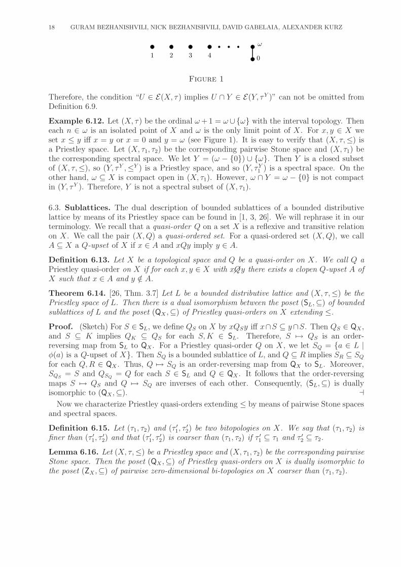
21 3 4

ω

0

Figure 1

Therefore, the condition “U ∈ E(X, τ) implies U ∩ Y ∈ E(Y, τY )” can not be omitted fromDefinition 6.9.

Example 6.12. Let (X, τ) be the ordinal ω+1 = ω∪{ω} with the interval topology. Theneach n ∈ ω is an isolated point of X and ω is the only limit point of X. For x, y ∈ X weset x ≤ y iff x = y or x = 0 and y = ω (see Figure 1). It is easy to verify that (X, τ,≤) isa Priestley space. Let (X, τ1, τ2) be the corresponding pairwise Stone space and (X, τ1) bethe corresponding spectral space. We let Y = (ω − {0}) ∪ {ω}. Then Y is a closed subsetof (X, τ,≤), so (Y, τY ,≤Y ) is a Priestley space, and so (Y, τY

1 ) is a spectral space. On theother hand, ω ⊆ X is compact open in (X, τ1). However, ω ∩ Y = ω − {0} is not compactin (Y, τY ). Therefore, Y is not a spectral subset of (X, τ1).

6.3. Sublattices. The dual description of bounded sublattices of a bounded distributivelattice by means of its Priestley space can be found in [1, 3, 26]. We will rephrase it in ourterminology. We recall that a quasi-order Q on a set X is a reflexive and transitive relationon X. We call the pair (X,Q) a quasi-ordered set. For a quasi-ordered set (X,Q), we callA ⊆ X a Q-upset of X if x ∈ A and xQy imply y ∈ A.

Definition 6.13. Let X be a topological space and Q be a quasi-order on X. We call Q aPriestley quasi-order on X if for each x, y ∈ X with xQ�y there exists a clopen Q-upset A ofX such that x ∈ A and y /∈ A.

Theorem 6.14. [26, Thm. 3.7] Let L be a bounded distributive lattice and (X, τ,≤) be thePriestley space of L. Then there is a dual isomorphism between the poset (SL,⊆) of boundedsublattices of L and the poset (QX ,⊆) of Priestley quasi-orders on X extending ≤.

Proof. (Sketch) For S ∈ SL, we define QS on X by xQSy iff x∩S ⊆ y∩S. Then QS ∈ QX ,and S ⊆ K implies QK ⊆ QS for each S,K ∈ SL. Therefore, S 7→ QS is an order-reversing map from SL to QX . For a Priestley quasi-order Q on X, we let SQ = {a ∈ L |φ(a) is a Q-upset of X}. Then SQ is a bounded sublattice of L, and Q ⊆ R implies SR ⊆ SQ

for each Q,R ∈ QX . Thus, Q 7→ SQ is an order-reversing map from QX to SL. Moreover,SQS

= S and QSQ= Q for each S ∈ SL and Q ∈ QX . It follows that the order-reversing

maps S 7→ QS and Q 7→ SQ are inverses of each other. Consequently, (SL,⊆) is duallyisomorphic to (QX ,⊆). ⊣

Now we characterize Priestley quasi-orders extending ≤ by means of pairwise Stone spacesand spectral spaces.

Definition 6.15. Let (τ1, τ2) and (τ ′1, τ′

2) be two bitopologies on X. We say that (τ1, τ2) isfiner than (τ ′1, τ

′

2) and that (τ ′1, τ′

2) is coarser than (τ1, τ2) if τ ′1 ⊆ τ1 and τ ′2 ⊆ τ2.

Lemma 6.16. Let (X, τ,≤) be a Priestley space and (X, τ1, τ2) be the corresponding pairwiseStone space. Then the poset (QX ,⊆) of Priestley quasi-orders on X is dually isomorphic tothe poset (ZX ,⊆) of pairwise zero-dimensional bi-topologies on X coarser than (τ1, τ2).


Proof. For a Priestley quasi-order Q on X, let τQ1 be the set of open Q-upsets and τQ

2

be the set of open Q-downsets of X. Clearly (τQ1 , τ

Q2 ) is a bi-topology on X coarser than

(τ1, τ2). Moreover, βQ1 = τQ

1 ∩δQ2 is exactly the set of clopen Q-upsets of X and βQ

2 = τQ2 ∩δ

Q1

is exactly the set of clopen Q-downsets of X. Since Q is a Priestley quasi-order, clopen Q-upsets are a basis for open Q-upsets and clopen Q-downsets are a basis for open Q-downsets.Therefore, (τQ

1 , τQ2 ) is pairwise zero-dimensional. For two Priestley quasi-orders Q and R on

X, we show Q ⊆ R implies τR1 ⊆ τQ

1 and τR2 ⊆ τQ

2 . Let U ∈ τR1 . Then U is an open R-upset

of X. Since Q ⊆ R, U is also a Q-upset of X. Thus, U ∈ τQ1 . That τR

2 ⊆ τQ2 is proved

similarly. It follows that Q 7→ (τQ1 , τ

Q2 ) is an order-reversing map from QX to ZX .

Let (τ ′1, τ′

2) be a pairwise zero-dimensional bi-topology onX coarser than (τ1, τ2). We defineQ(τ ′

1,τ ′

2)to be the specialization order of τ ′1. Since (τ ′1, τ

′

2) is pairwise zero-dimensional, Q(τ ′

1,τ ′

2)

is the dual of the specialization order of τ ′2. Because Q(τ ′

1,τ ′

2) is a specialization order, it is clearthat Q(τ ′

1,τ ′

2)is a quasi-order. From τ ′1 ⊆ τ1 it follows that Q(τ ′

1,τ ′

2) extends the specializationorder of τ1. Consequently, Q(τ ′

1,τ ′

2)extends ≤. We show that Q(τ ′

1,τ ′

2)is a Priestley quasi-order.

If xQ�(τ ′

1,τ ′

2)y, then there exists U ∈ τ ′1 such that x ∈ U and y /∈ U . Since (τ ′1, τ

′

2) is pairwisezero-dimensional, we may assume that U ∈ β ′

1. Therefore, U is clopen in τ . Clearly eachU ∈ τ ′1 is a Q(τ ′

1,τ ′

2)-upset. Thus, there exists a clopen Q(τ ′

1,τ ′

2)-upset U of X such that x ∈ U

and y /∈ U . For (τ ′1, τ′

2), (τ′′

1 , τ′′

2 ) ∈ ZX , we show (τ ′1, τ′

2) ⊆ (τ ′′1 , τ′′

2 ) implies Q(τ ′′

1 ,τ ′′

2 ) ⊆ Q(τ ′

1,τ ′

2).

Let xQ(τ ′′

1 ,τ ′′

2 )y. Then x ∈ U implies y ∈ U for each U ∈ τ ′′1 . Therefore, x ∈ U implies y ∈ Ufor each U ∈ τ ′1. Thus, xQ(τ ′

1,τ ′

2)y. It follows that (τ ′1, τ

′

2) 7→ Q(τ ′

1,τ ′

2) is an order-reversing mapfrom ZX to QX .

We show that Q(τQ1 ,τ

Q2 ) = Q and (τ

Q(τ ′1

,τ ′2)

1 , τQ(τ ′

1,τ ′

2)

2 ) = (τ ′1, τ′

2) for each Q ∈ QX and (τ ′1, τ′

2) ∈

ZX . Indeed, xQ(τQ1 ,τ

Q2 )y iff (∀U ∈ τQ

1 )(x ∈ U ⇒ y ∈ U), which is equivalent to xQy since

Q is a Priestley quasi-order. Thus, Q(τQ1 ,τ

Q2 ) = Q. Moreover, U ∈ τ

Q(τ ′1,τ ′2)

1 iff U is an open

Q(τ ′

1,τ ′

2)-upset of X. Clearly U ∈ τ ′1 implies U is an open Q(τ ′

1,τ ′

2)-upset of X. Conversely,

let U be an open Q(τ ′

1,τ ′

2)-upset of X. We show that U =⋃{V ∈ τ ′1 | V ⊆ U}. Clearly⋃

{V ∈ τ ′1 | V ⊆ U} ⊆ U . Let x ∈ U . Since U is a Q(τ ′

1,τ ′

2)-upset, for each y ∈ U c we

have xQ�(τ ′

1,τ ′

2)y. Therefore, there exists Vy ∈ τ ′1 such that x ∈ Vy and y /∈ Vy. Since β ′

1

is a basis for τ ′1, we may assume that Vy ∈ β ′

1. Thus,⋂{Vy | y ∈ U c} ∩ U c = ∅. Since

U c and each Vy is closed in τ and τ is compact, there exist V1, . . . , Vn ∈ β ′

1 such thatV1 ∩ · · · ∩ Vn ∩ U

c = ∅. So x ∈ V1 ∩ · · · ∩ Vn ⊆ U c, and so U ⊆⋃{V ∈ τ ′1 | V ⊆ U}.

Consequently, U ∈ τ ′1. This implies that τQ(τ ′

1,τ ′

2)

1 = τ ′1. A similar argument shows that

τQ(τ ′

1,τ ′

2)

2 = τ ′2. Thus, (τQ(τ ′

1,τ ′

2)

1 , τQ(τ ′

1,τ ′

2)

2 ) = (τ ′1, τ′

2). It follows that the order-reversing maps

Q 7→ (τQ1 , τ

Q2 ) and (τ ′1, τ

′

2) 7→ Q(τ ′

1,τ ′

2) are inverses of each other. Thus, (QX ,⊆) is duallyisomorphic to (ZX ,⊆). ⊣

Definition 6.17. Let τ be a spectral topology on X and let τ ′ be a coherent topology on Xcoarser than τ . We call τ ′ strongly coherent if the set E(X, τ ′) of compact open subsets of(X, τ ′) is equal to the set τ ′ ∩ σ of open subsets of (X, τ ′) that are compact in (X, τ).

Lemma 6.18. Let (X, τ1, τ2) be a pairwise Stone space and (X, τ1) be the correspondingspectral space. Then the poset (ZX ,⊆) of pairwise zero-dimensional bi-topologies (τ ′1, τ

′

2) onX coarser than (τ1, τ2) is isomorphic to the poset (SCX ,⊆) of strongly coherent topologies τ ′1on X coarser than τ1.


Proof. Let (τ ′1, τ′

2) be a pairwise zero-dimensional bi-topology on X coarser than (τ1, τ2).Then τ ′1 is a topology on X coarser than τ1. Let β ′

1 = τ ′1∩ δ′

2. We show that E(X, τ ′1) = β ′

1 =τ ′1∩σ1. Let U ∈ E(X, τ ′1). Since β ′

1 is a basis for τ ′1, U is the union of elements of β ′

1 containedin U . As U is compact in (X, τ ′1), U is a finite union of elements of β ′

1, so U is an element ofβ ′

1, and so E(X, τ ′1) ⊆ β ′

1. Now let U ∈ β ′

1. Because (X, τ1, τ2) is pairwise compact, δ2 ⊆ σ1.Therefore, δ′2 ⊆ δ2 ⊆ σ1, and so β ′

1 ⊆ τ ′1 ∩ δ′

2 ⊆ τ ′1 ∩ σ1. Finally, let U ∈ τ ′1 ∩ σ1. Since U ∈ τ ′1and E(X, τ ′1) is a basis for τ ′1, U is the union of elements of E(X, τ ′1) contained in U . BecauseU ∈ σ1 and τ ′1 ⊆ τ1, U is a finite union of elements of E(X, τ ′1). Therefore, U ∈ E(X, τ ′1), andso τ ′1 ∩ σ1 ⊆ E(X, τ

′

1). Thus, E(X, τ ′1) = β ′

1 = τ ′1 ∩ σ1, implying that τ ′1 is a strongly coherenttopology. For (τ ′1, τ

′

2), (τ′′

1 , τ′′

2 ) ∈ ZX , if (τ ′1, τ′

2) ⊆ (τ ′′1 , τ′′

2 ), then it is obvious that τ ′1 ⊆ τ ′′1 . Itfollows that (τ ′1, τ

′

2) 7→ τ ′1 is an order-preserving map from ZX to SCX .For a strongly coherent topology τ ′1 on X coarser than τ1, we let τ ′2 be the topology

generated by the basis ∆(X, τ ′1) = {U c | U ∈ E(X, τ ′1)}. Let δ′1 denote the set of closedsubsets of (X, τ ′1) and δ′2 denote the set of closed subsets of (X, τ ′2). We set β ′

1 = τ ′1 ∩ δ′

2 andβ ′

2 = τ ′2 ∩ δ′

1. We show that β ′

1 = E(X, τ ′1) and β ′

2 = ∆(X, τ ′1). It follows from the definitionthat E(X, τ ′1) ⊆ β ′

1. Conversely, β ′

1 = τ ′1 ∩ δ′

2 ⊆ τ ′1 ∩ δ2 ⊆ τ ′1 ∩ σ1 = E(X, τ ′1). Therefore,β ′

1 = E(X, τ ′1). Also, U ∈ ∆(X, τ ′1) iff U c ∈ E(X, τ ′1) iff U c ∈ β ′

1 iff U c ∈ τ ′1 ∩ δ′

2 iff U ∈ δ′1 ∩ τ′

2

iff U ∈ β ′

2. Thus, β ′

2 = ∆(X, τ ′1). Consequently, β ′

1 is a basis for τ ′1 and β ′

2 is a basis forτ ′2, and so (τ ′1, τ

′

2) is pairwise zero-dimensional. For τ ′1, τ′′

1 ∈ SCX , we show τ ′1 ⊆ τ ′′1 implies(τ ′1, τ

′

2) ⊆ (τ ′′1 , τ′′

2 ). Let U ∈ ∆(X, τ ′1). Then U c ∈ E(X, τ ′1). Therefore, U c ∈ τ ′1∩σ1 ⊆ τ ′′1 ∩σ1,and so U c ∈ E(X, τ ′′1 ). Thus, U ∈ ∆(X, τ ′′1 ), so ∆(X, τ ′1) ⊆ ∆(X, τ ′′1 ), and so τ ′2 ⊆ τ ′′2 . Itfollows that τ ′1 7→ (τ ′1, τ

′

2) is an order-preserving map from SCX to ZX .Finally, if (τ ′1, τ

′

2) ∈ ZX , then E(X, τ ′1) = β ′

1, so ∆(X, τ ′1) = β ′

2, and so the compositionZX → SCX → ZX is an identity. Moreover, it is clear that the composition SCX → ZX →SCX is also an identity. Thus, (ZX ,⊆) is isomorphic to (SCX ,⊆). ⊣

Putting Theorem 6.14 and Lemmas 6.16 and 6.18 together, we obtain the following dualdescription of bounded sublattices of L by means of all three dual spaces of L.

Corollary 6.19. Let L be a bounded distributive lattice, (X, τ,≤) be the Priestley space of L,(X, τ1, τ2) be the pairwise Stone space of L, and (X, τ1) be the spectral space of L. Then theposet (SL,⊆) of bounded sublattices of L is dually isomorphic to the poset (QX ,⊆) of Priestleyquasi-orders on X extending ≤, and is isomorphic to the poset (ZX ,⊆) of pairwise zero-dimensional bi-topologies on X coarser than (τ1, τ2), and to the poset (SCX ,⊆) of stronglycoherent topologies on X coarser than τ1.

6.4. Canonical completions, MacNeille completions, and complete lattices. In thetheory of completions of lattices, or more generally of posets, the MacNeille and canonicalcompletions play a prominent role. Let L be a lattice. We recall that a subset S of L isjoin-dense in L if for each a ∈ L we have a =

∨(↓a ∩ S), and that S is meet-dense in L

if for each a ∈ L we have a =∧

(↑a ∩ S). We further recall that the MacNeille completionof L is a unique up to isomorphism complete lattice L together with a lattice embeddingi : L→ L such that i[L] is both join-dense and meet-dense in L. Furthermore, we recall thatthe canonical completion of L is a unique up to isomorphism complete lattice Lσ togetherwith a lattice embedding j : L → Lσ such that (i) for each filter F and ideal I of L, fromF ∩ I = ∅ it follows that

∧j[F ] 6≤

∨j[I], (ii) the set KL = {

∧j[S] | S ⊆ L} of closed

elements of Lσ is join-dense in Lσ, and (iii) the set OL = {∨j[S] | S ⊆ L} of open elements

of Lσ is meet-dense in Lσ.


For a Priestley space (X, τ,≤), following [11, Sec. 3], we define two maps D : OpUp(X)→ClUp(X) and J : ClUp(X) → OpUp(X) by D(U) = ↑Cl(U) and J(K) = (↓(IntK)c)c forU ∈ OpUp(X) and K ∈ ClUp(X). Then it follows from [11, Lemma 3.4] that D and J forma Galois connection between (OpUp(X),⊆) and (ClUp(X),⊇). Let RgOpUp(X) denote theset of fixpoints of J ◦ D; that is, RgOpUp(X) = {U ∈ OpUp(X) | JDU = U}. The nexttheorem is well-known. The first half of it can be found in [11, Thm. 3.5], and the secondhalf in [9, Sec. 2].

Theorem 6.20. Let L be a bounded distributive lattice and (X, τ,≤) be the Priestley spaceof L. Then L is isomorphic to RgOpUp(X) and Lσ is isomorphic to Up(X).

Let L be a bounded distributive lattice, (X, τ,≤) be the Priestley space of L, (X, τ1, τ2)be the pairwise Stone space of L, and (X, τ1) be the spectral space of L. Since Up(X) =S1(X) = CS2(X), we immediately obtain the following dual description of the canonicalcompletion of L.

Theorem 6.21. Let L be a bounded distributive lattice, (X, τ,≤) be the Priestley space ofL, (X, τ1, τ2) be the pairwise Stone space of L, and (X, τ1) be the spectral space of L. ThenLσ is isomorphic to Up(X) = S1(X) = CS2(X).

Let L be a bounded distributive lattice, (X, τ,≤) be the Priestley space of L, and (X, τ1, τ2)be the pairwise Stone space of L. Since OpUp(X) = τ1, ClUp(X) = δ2, D(U) = Cl2(U),and J(U) = Int1(U) for U ⊆ X, we obtain that Cl2 : τ1 → δ2 and Int1 : δ2 → τ1 form aGalois connection between (τ1,⊆) and (δ2,⊇), and so the MacNeille completion L of L isisomorphic to the fixpoints of Int1 ◦ Cl2, we denote by RgOp12(X).

Let (X, τ1) be the spectral space corresponding to the pairwise Stone space (X, τ1, τ2).Then δ2 = KS1(X) and Cl2(U) = Sat1Cl(U) for U ⊆ X. Let S1 = Sat1 ◦ Cl. ThenS1 : τ1 → KS1(X) and Int1 : KS1(X) → τ1 form a Galois connection between (τ1,⊆) and(KS1(X),⊇), and so the MacNeille completion L of L is isomorphic to the fixpoints ofInt1 ◦ S1, we denote by SatOp1(X). Consequently, we obtain the following dual descriptionof the MacNeille completion of L.

Theorem 6.22. Let L be a bounded distributive lattice, (X, τ,≤) be the Priestley space ofL, (X, τ1, τ2) be the pairwise Stone space of L, and (X, τ1) be the spectral space of L. ThenL is isomorphic to RgOpUp(X) = RgOp12(X) = SatOp1(X).

The bitopological description of L provides a nice generalization of the characterizationof the MacNeille completion of a Boolean algebra B by means of the regular open subsetsof the Stone space (X, τ) of B. We recall that the regular open subsets of (X, τ) are exactlythe fixpoints of the maps Cl : τ → δ and Int : δ → τ . When working with a pairwiseStone space (X, τ1, τ2), we consider the fixpoints of the maps Cl2 and Int1 between τ1 andδ2, respectively. Therefore, whenever τ1 = τ2, the pairwise Stone space (X, τ1, τ2) becomesthe Stone space (X, τ), where τ = τ1 = τ2. So τ1 = τ , δ2 = δ, Cl2 = Cl, Int1 = Int, andthe fixpoints of Int1 ◦ Cl2 are exactly the regular open subsets of (X, τ). As a corollary, weobtain the well-known dual description of the MacNeille completion of a Boolean algebra:

Corollary 6.23. Let B be a Boolean algebra and (X, τ) be the Stone space of B. Then theMacNeille completion B of B is isomorphic to the regular open subsets RgOp(X, τ) of (X, τ).

Since L is a complete lattice iff L is isomorphic to L, it follows from the construction ofL that L is complete iff in the dual Priestley space (X, τ,≤) of L we have RgOpUp(X) =


DLat Pries PStone Spec

filter closed upset τ2-closed set compact saturated set

ideal open upset τ1-open set open set

prime filter ↑x Cl2(x) Sat(x)

prime ideal (↓x)c [Cl1(x)]c [Cl(x)]c

maximal filter ↑x = {x} Cl2(x) = {x} Sat(x) = {x}

maximal ideal (↓x)c = {x}c [Cl1(x)]c = {x}c [Cl(x)]c = {x}c

homomorphic image closed subset pairwise compact subset spectral subset

subalgebra Q ∈ QX (τ ′

1, τ′

2) ∈ ZX τ ′ ∈ SCX

canonical completion Up(X) S1(X) = CS2(X) S(X)

MacNeille complition RgOpUp(X) RgOp12(X) SatOp(X)

complete lattice RgOpUp(X) = CpUp(X) β1 = RgOp12(X) E(X) = SatOp(X)

Table 1. Dictionary for DLat, Pries, PStone, and Spec.

ClUp(X) (see [21, Prop. 16] and [11, p. 948]). Such Priestley spaces were called extremallyorder disconnected in [21, p. 521]. This together with Theorem 6.22 immediately give us thefollowing dual description of complete distributive lattices.

Theorem 6.24. Let L be a bounded distributive lattice, (X, τ,≤) be the Priestley space ofL, (X, τ1, τ2) be the pairwise Stone space of L, and (X, τ1) be the spectral space of L. Thenthe following conditions are equivalent:

(1) L is complete.(2) RgOpUp(X) = ClUp(X).(3) RgOp12(X) = β1.(4) SatOp1(X) = E(X, τ1).

In Table 1 we gather together the dual descriptions of different algebraic concepts forbounded distributive lattices by means of their Priestley spaces, pairwise Stone spaces, andspectral spaces obtained in this section. This can be thought of as a dictionary of dualitytheory for bounded distributive lattices, complementing the dictionary given in [22].

7. Duality for Heyting algebras, co-Heyting algebras, and bi-Heyting

algebras

A rather natural subclass of distributive lattices is the class of Heyting algebras (resp.co-Heyting algebras/bi-Heyting algebras), which plays an important role in the study of su-perintuitionistic logics. The first duality for Heyting algebras (resp. co-Heyting algebras/bi-Heyting algebras) was developed by Esakia [5] (resp. [6]). It is a restricted version of Priest-ley’s duality. In this section we develop duality for Heyting algebras (resp. co-Heytingalgebras/bi-Heyting algebras) by means of pairwise Stone spaces and spectral spaces, thusproviding the bitopological and spectral alternatives of the Esakia duality.

We recall that a Heyting algebra is a bounded distributive lattice (A,∧,∨, 0, 1) with abinary operation →: A2 → A such that for all a, b, c ∈ A we have:

c ≤ a→ b iff a ∧ c ≤ b.

Similarly a co-Heyting algebra is a bounded distributive lattice A with a binary operation←: A2 → A such that for all a, b, c ∈ A we have:

c ≥ a← b iff b ∨ c ≥ a.


We call (A,→,←) a bi-Heyting algebra if (A,→) is a Heyting algebra and (A,←) is a co-Heyting algebra.

Let A and A′ be two Heyting algebras. We recall that a map h : A → A′ is a Heytingalgebra homomorphism if h is a bounded lattice homomorphism and h(a→ b) = h(a)→′ h(b)for each a, b ∈ A. Similarly, if A and A′ are two co-Heyting algebras, then h : A → A′ isa co-Heyting algebra homomorphism if h is a bounded lattice homomorphism and h(a ←b) = h(a) ←′ h(b) for each a, b ∈ A. If A and A′ are two bi-Heyting algebras, then h isa bi-Heyting algebra homomorphism if it is both a Heyting algebra homomorphism and aco-Heyting algebra homomorphism. Let Heyt denote the category of Heyting algebras andHeyting algebra homomorphisms, coHeyt denote the category of co-Heyting algebras andco-Heyting algebra homomorphisms, and biHeyt denote the category of bi-Heyting algebrasand bi-Heyting algebra homomorphisms. Clearly biHeyt = Heyt ∩ coHeyt.

For a topological space (X, τ), let Cp(X) denote the set of clopen subsets of X.

Definition 7.1. Let (X, τ,≤) be a Priestley space.

(1) We call (X, τ,≤) an Esakia space if A ∈ Cp(X) implies ↓A ∈ Cp(X).(2) We call (X, τ,≤) a co-Esakia space if A ∈ Cp(X) implies ↑A ∈ Cp(X).(3) We call (X, τ,≤) a bi-Esakia space if it is both an Esakia space and a co-Esakia

space.

Let (X,≤) and (X ′,≤′) be two posets. We recall that a map f : X → X ′ is a p-morphismif it is order-preserving and for each x ∈ X and x′ ∈ X ′, from f(x) ≤ x′ it follows thatthere is y ∈ X such that x ≤ y and f(y) = x′. We call f : X → X ′ a co-p-morphism if itis order-preserving and for each x ∈ X and x′ ∈ X ′, from x′ ≤ f(x) it follows that thereis y ∈ X such that y ≤ x and f(y) = x′. For two Esakia spaces (resp. co-Esakia spaces)(X, τ,≤) and (X ′, τ ′,≤′), we call a map f : X → X ′ an Esakia morphism (resp. a co-Esakiamorphism) if it is a continuous p-morphism (resp. a continuous co-p-morphism). We call fa bi-Esakia morphism if it is both an Esakia morphism and a co-Esakia morphism. Let Esa

denote the category of Esakia spaces and Esakia morphisms, coEsa denote the categoryof co-Esakia spaces and co-Esakia morphisms, and biEsa denote the category of bi-Esakiaspaces and bi-Esakia morphisms. Then we have the following theorem established in [5] and[6]:

Theorem 7.2. Heyt is dually equivalent to Esa, coHeyt is dually equivalent to coEsa,and biHeyt is dually equivalent to biEsa.

In fact, the same functors establishing the dual equivalence of DLat and Pries restricted toHeyt (resp. coHeyt/biHeyt) establish the required dual equivalences. In order to describethe pairwise Stone spaces and spectral spaces dual to Heyting algebras (resp. coHeytingalgebras/bi-Heyting algebras), it is sufficient to characterize those pairwise Stone spaces andspectral spaces that correspond to Esakia spaces (resp. coEsakia spaces/biEsakia spaces).As an immediate consequence of Lemma 6.8 and Theorem 6.10, we obtain:

Lemma 7.3. Let (X, τ,≤) be a Priestley space, (X, τ1, τ2) be the corresponding pairwiseStone space, and (X, τ1) be the corresponding spectral space. For Y ⊆ X, the followingconditions are equivalent:

(1) Y is clopen in (X, τ,≤).(2) Y and Y c are pairwise compact in (X, τ1, τ2).(3) Y and Y c are spectral subsets of (X, τ1).


Let (X, τ1, τ2) be a pairwise Stone space. We call Y ⊆ X doubly pairwise compact if bothY and Y c are pairwise compact in (X, τ1, τ2). Let DPC(X) denote the set of doubly pairwisecompact subsets of (X, τ1, τ2).

Definition 7.4. Let (X, τ1, τ2) be a pairwise Stone space.

(1) We call (X, τ1, τ2) a Heyting bitopological space if A ∈ DPC(X) implies Cl1(A) ∈DPC(X).

(2) We call (X, τ1, τ2) a co-Heyting bitopological space if A ∈ DPC(X) implies Cl2(A) ∈DPC(X).

(3) We call (X, τ1, τ2) a bi-Heyting bitopological space if it is both a Heyting bitopologicalspace and a co-Heyting bitopological space.

Theorem 7.5. Let (X, τ1, τ2) be a pairwise Stone space.

(1) (X, τ1, τ2) is a Heyting bitopological space iff for each A ∈ β1 and B ∈ β2 we haveCl1(A ∩B) ∈ β2.

(2) (X, τ1, τ2) is a co-Heyting bitopological space iff for each A ∈ β1 and B ∈ β2 we haveCl2(A ∩B) ∈ β1.

(3) (X, τ1, τ2) is a bi-Heyting bitopological space iff for each A ∈ β1 and B ∈ β2 we haveCl1(A ∩B) ∈ β2 and Cl2(A ∩ B) ∈ β1.

Proof. (1) Let (X, τ,≤) be the Priestley space corresponding to (X, τ1, τ2). Suppose that(X, τ1, τ2) is a Heyting bitopological space, A ∈ β1, and B ∈ β2. Then A ∈ δ2 and Ac ∈ δ1.Therefore, both A and Ac are closed in (X, τ,≤). A similar argument shows that both Band Bc are closed in (X, τ,≤). Thus, both A ∩ B and (A ∩ B)c = Ac ∪ Bc are closed in(X, τ,≤). By Lemma 6.8, both A ∩ B and (A ∩ B)c are pairwise compact in (X, τ,≤),implying that A ∩ B ∈ DPC(X). Since (X, τ1, τ2) is a Heyting bitopological space, wehave Cl1(A ∩ B) ∈ DPC(X). By Lemma 7.3, Cl1(A ∩ B) is clopen in (X, τ,≤). Moreover,since ≤ is the specialization order of (X, τ1), we have that Cl1(A ∩ B) is a downset of(X, τ,≤). Therefore, Cl1(A ∩ B) ∈ CpDo(X). By Proposition 3.4, CpDo(X) = β2. Thus,Cl1(A ∩ B) ∈ β2.

Conversely, suppose that (X, τ1, τ2) is a pairwise Stone space and for each A ∈ β1 andB ∈ β2 we have Cl1(A ∩ B) ∈ β2. Let A ∈ DPC(X). By Lemma 7.3, A is clopen in(X, τ,≤). Since CpUp(X)∪CpDo(X) is a subbasis for τ and A is compact in (X, τ), we haveA = (U1 ∩ V1) ∪ · · · ∪ (Un ∩ Vn) for some U1, . . . , Un ∈ CpUp(X) and V1, . . . , Vn ∈ CpDo(X).By Proposition 3.4, CpUp(X) = β1 and CpDo(X) = β2. Therefore, for each i = 1, . . . , n wehave Cl1(Ui ∩ Vi) ∈ β2. Thus, Cl1(A) = Cl1[(U1 ∩ V1) ∪ · · · ∪ (Un ∩ Vn)] = Cl1(U1 ∩ V1) ∪· · · ∪ Cl1(Un ∩ Vn) ∈ β2 = CpDo(X). This implies that Cl1(A) is clopen in (X, τ,≤), so byLemma 7.3, Cl1(A) ∈ DPC(X), and so (X, τ1, τ2) is a Heyting bitopological space.

(2) is proved similarly.(3) is an immediate consequence of (1) and (2). ⊣

From now on we will call a pairwise Stone space a Heyting bitopological space (resp.co-Heyting bitopological space/bi-Heyting bitopological space) if it satisfies the condition ofTheorem 7.5.1 (resp. Theorem 7.5.2/Theorem 7.5.3).

Theorem 7.6. Let (X, τ,≤) be a Priestley space and (X, τ1, τ2) be the corresponding pairwiseStone space. Then:

(1) (X, τ,≤) is an Esakia space iff (X, τ1, τ2) is a Heyting bitopological space.(2) (X, τ,≤) is a co-Esakia space iff (X, τ1, τ2) is a co-Heyting bitopological space.


(3) (X, τ,≤) is a bi-Esakia space iff (X, τ1, τ2) is a bi-Heyting bitopological space.

Proof. Since Cp(X) = DPC(X) and for A ∈ DPC(X) we have Cl1(A) = ↓A and Cl2(A) =↑A, the results follow. ⊣

In order to characterize morphisms between Esakia (resp. co-Esakia) bitopological spaces,we recall the following characterization of p-morphisms (resp. co-p-morphisms).

Lemma 7.7. [7, pp. 17-18] For two posets (X,≤) and (X ′,≤′) and a map f : X → X ′, thefollowing conditions are equivalent:

(1) f is a p-morphism (resp. f is a co-p-morphism).(2) For each x ∈ X we have f(↑x) = ↑f(x) (resp. f(↓x) = ↓f(x)).(3) For each x′ ∈ X ′ we have f−1(↓x′) = ↓f−1(x′) (resp. f−1(↑x′) = ↑f−1(x′)).

Definition 7.8.

(1) Let (X, τ1, τ2) and (X ′, τ ′1, τ′

2) be two Heyting bitopological spaces. We call a mapf : X → X ′ a Heyting morphism if f is bi-continuous and f(Cl2(x)) = Cl′2(f(x)) foreach x ∈ X.

(2) Let (X, τ1, τ2) and (X ′, τ ′1, τ′

2) be two co-Heyting bitopological spaces. We call a mapf : X → X ′ a co-Heyting morphism if f is bi-continuous and f(Cl1(x)) = Cl′1(f(x))for each x ∈ X.

(3) Let (X, τ1, τ2) and (X ′, τ ′1, τ′

2) be two bi-Heyting bitopological spaces. We call a mapf : X → X ′ a bi-Heyting morphism if f is bi-continuous, f(Cl2(x)) = Cl′2(f(x)),and f(Cl1(x)) = Cl′1(f(x)) for each x ∈ X.

Let (X, τ,≤) and (X ′, τ ′,≤′) be two Esakia spaces, (X, τ1, τ2) and (X ′, τ ′1, τ′

2) be the cor-responding Heyting bitopological spaces, and f : X → X ′ be bi-continuous. By Corollary6.5, for each x ∈ X we have ↑x = Cl2(x) and ↓x = Cl1(x). Therefore, by Lemma 7.7, fis an Esakia morphism iff f is a Heyting morphism iff f−1(Cl1(x

′)) = Cl1(f−1(x′)). Simi-

larly, for two co-Esakia spaces (X, τ,≤) and (X ′, τ ′,≤′) and their corresponding co-Heytingbitopological spaces (X, τ1, τ2) and (X ′, τ ′1, τ

′

2), a bi-continuous map f : X → X ′ is a co-Esakia morphism iff f is a co-Heyting morphism iff f−1(Cl2(x

′)) = Cl2(f−1(x′)). Putting

these together, for two bi-Esakia spaces (X, τ,≤) and (X ′, τ ′,≤′) and their correspondingbi-Heyting bitopological spaces (X, τ1, τ2) and (X ′, τ ′1, τ

′

2), a bi-continuous map f : X → X ′

is a bi-Esakia morphism iff f is a bi-Heyting morphism iff f−1(Cl1(x′)) = Cl1(f

−1(x′)) andf−1(Cl2(x

′)) = Cl2(f−1(x′)).

Let HPStone denote the category of Heyting bitopological spaces and Heyting mor-phisms, coHPStone denote the category of co-Heyting bitopological spaces and co-Heytingmorphisms, and biHPStone denote the category of bi-Heyting bitopological spaces andbi-Heyting morphisms. Clearly each of HPStone, coHPStone, and HPStone is a propersubcategory of PStone. Moreover, biHPStone = HPStone∩ coHPStone. Furthermore,putting the results obtained above together, we obtain:

Theorem 7.9.

(1) The categories Esa and HPStone are isomorphic. Consequently, Heyt is duallyequivalent to HPStone.

(2) The categories coEsa and coHPStone are isomorphic. Consequently, coHeyt isdually equivalent to coHPStone.

(3) The categories biEsa and biHPStone are isomorphic. Consequently, biHeyt isdually equivalent to biHPStone.


Let (X, τ) be a spectral space. We call Y ⊆ X a doubly spectral subset of (X, τ) if both Yand Y c are spectral subsets of (X, τ). Let DS(X) denote the set of doubly spectral subsetsof X.

Definition 7.10. Let (X, τ) be a spectral space.

(1) We call (X, τ) H-spectral if A ∈ DS(X) implies Cl(A) ∈ DS(X).(2) We call (X, τ) coH-spectral if A ∈ DS(X) implies Sat(A) ∈ DS(X).(3) We call (X, τ) biH-spectral if it is both H-spectral and coH-spectral.

Theorem 7.11. Let (X, τ1, τ2) be a pairwise Stone space and (X, τ1) be the correspondingspectral space. Then:

(1) (X, τ1, τ2) is a Heyting bitopological space iff (X, τ1) is H-spectral.(2) (X, τ1, τ2) is a co-Heyting bitopological space iff (X, τ1) is coH-spectral.(3) (X, τ1, τ2) is a bi-Heyting bitopological space iff (X, τ1) is biH-spectral.

Proof. By Lemma 7.3, DPC(X) = DS(X). The results follow. ⊣

For two H-spectral spaces (X, τ) and (X ′, τ ′), we call a map f : X → X ′ H-spectral if fis spectral and f(Sat(x)) = Sat′(f(x)). Moreover, for two coH-spectral spaces (X, τ) and(X ′, τ ′), we call a map f : X → X ′ coH-spectral if f is spectral and f(Cl(x)) = Cl′(f(x)).Furthermore, for two biH-spectral spaces (X, τ) and (X ′, τ ′), we call a map f : X → X ′

biH-spectral if f is spectral, f(Sat(x)) = Sat′(f(x)), and f(Cl(x)) = Cl′(f(x)).Let (X, τ1, τ2) and (X ′, τ ′1, τ

′

2) be two Heyting bitopological spaces and (X, τ1) and (X ′, τ ′1)be the corresponding H-spectral spaces. By Corollary 6.5, for each x ∈ X we have Cl2(x) =Sat1(x) and Cl1(x) = Sat2(x). Therefore, a bi-continuous map f : X → X ′ is a Heytingmorphism iff f is H-spectral iff f−1(Cl1(x

′)) = Cl1(f−1(x′)). Similarly, for two co-Heyting

bitopological spaces (X, τ1, τ2) and (X ′, τ ′1, τ′

2) and their corresponding coH-spectral spaces(X, τ1) and (X ′, τ ′1), a bi-continuous map f : X → X ′ is a co-Heyting morphism iff f iscoH-spectral iff f−1(Sat1(x

′)) = Sat1(f−1(x′)). Putting these together, for two bi-Heyting

bitopological spaces (X, τ1, τ2) and (X ′, τ ′1, τ′

2) and their corresponding biH-spectral spaces(X, τ1) and (X ′, τ ′1), a bi-continuous map f : X → X ′ is a bi-Heyting morphism iff f isbiH-spectral iff f−1(Sat1(x

′)) = Sat1(f−1(x′)) and f−1(Cl1(x

′)) = Cl1(f−1(x′)).

Let HSpec denote the category of H-spectral spaces and H-spectral maps, coHSpec

denote the category of coH-spectral spaces and coH-spectral maps, and biHSpec denote thecategory of biH-spectral spaces and biH-spectrals maps. Clearly each of HSpec, coHSpec,and biHSpec is a proper subcategory of Spec. Moreover, biHSpec = HSpec∩coHSpec.Furthermore, putting the results obtained above together, we obtain:

Theorem 7.12.

(1) The categories Esa, HPStone, and HSpec are isomorphic. Consequently, Heyt isalso dually equivalent to HSpec.

(2) The categories coEsa, coHPStone, and coHSpec are isomorphic. Consequently,coHeyt is also dually equivalent to coHSpec.

(3) The categories biEsa, biHPStone, and biHSpec are isomorphic. Consequently,biHeyt is also dually equivalent to biHSpec.

The dual description of algebraic concepts important for the study of Heyting algebras(resp. co-Heyting algebras/bi-Heyting algebras) is similar to that of bounded distributivelattices. The dual description of filters, prime filters, and maximal filters as well as ideals,


prime ideals, and maximal ideals is exactly the same. So is the dual description of thecanonical completions. On the other hand, the dual description of the MacNeille completionsgets simplified [11, Sec. 3]: In the case of Heyting algebras, we have D = Cl; and in the caseof co-Heyting algebras, we have J = Int; consequently, in the case of bi-Heyting algebras weobtain that Cl and Int form a Galois connection between OpUp(X) and ClOp(X), and so theMacNeille completion A of a bi-Heyting algebra is dually characterized as the fixpoints ofCl ◦ Int, which are exactly the regular open upsets of X. This provides a nice generalizationof the Boolean case (see Corollary 6.23).

It is well-known that homomorphic images of a Heyting algebra A are characterized by itsfilters. Consequently, unlike the case of bounded distributive lattices, homomorphic imagesof a Heyting algebra A dually correspond to closed upsets of the Esakia space X of A.Similarly, homomorphic images of a co-Heyting algebra A are characterized by its ideals,and so homomorphic images of A dually correspond to open upsets of the co-Esakia spaceX of A. Therefore, homomorphic images of a bi-Heyting algebra A dually correspond toeither closed upsets that are also downsets (denoted ClUpDo(X)) or open upsets that arealso downsets (denoted OpUpDo(X)) of the bi-Esakia space X of A, thus generalizing theBoolean case, where homomorphic images of a Boolean algebra B dually correspond to eitherclosed subsets or open subsets of the Stone space X of B. We give the dual description ofsubalgebras of a Heyting algebra (resp. co-Heyting algebra/bi-Heyting algebra). For a quasi-ordered set (X,Q), we define an equivalence relation E on X by xEy iff xQy and yQx.

Definition 7.13. Let (X, τ,≤) be a Priestley space and Q be a Priestley quasi-order on Xextending ≤.

(1) We call Q an Esakia quasi-order if for each x, y ∈ X, from xQy it follows that thereexists z ∈ X such that x ≤ z and zEy.

(2) We call Q a co-Esakia quasi-order if for each x, y ∈ X, from xQy it follows thatthere exists u ∈ X such that xEu and u ≤ y.

(3) We call Q a bi-Esakia quasi-order if Q is both an Esakia quasi-order and a co-Esakiaquasi-order.

Remark 7.14. Let (X, τ,≤) be a Priestley space and E be an equivalence relation on X.We call E an Esakia (resp. co-Esakia) equivalence relation if E viewed as a quasi-order is aPriestley quasi-order on X and ↑E(x) ⊆ E(↑x) (resp. ↓E(x) ⊆ E(↓x)). We also call E a bi-Esakia equivalence relation if E is both an Esakia and a co-Esakia equivalence relation. It iseasy to see that if Q is an Esakia (resp. co-Esakia/bi-Esakia) quasi-order, then E is an Esakia(resp. co-Esakia/bi-Esakia) equivalence relation. For an Esakia (resp. co-Esakia) equivalencerelation E, we define Q on X by xQy iff there exists z ∈ X such that x ≤ z and zEy (resp.there exists u ∈ X such that xEu and u ≤ y). Then for an Esakia (resp. co-Esakia) spaceX, it is easy to see that Q is an Esakia (resp. co-Esakia) quasi-order. Also if X is a bi-Esakia space and E is a bi-Esakia equivalence relation, then Q is a bi-Esakia quasi-order.Thus, for an Esakia (resp. co-Esakia/bi-Esakia) space X, there is an isomorphism betweenEsakia (resp. co-Esakia/bi-Esakia) quasi-orders on X ordered by inclusion and Esakia (resp.co-Esakia/bi-Esakia) equivalence relations on X ordered by inclusion.

Theorem 7.15.

(1) Let A be a Heyting algebra and (X, τ,≤) be the Esakia space of A. Then the poset(HSA,⊆) of Heyting subalgebras of A is dually isomorphic to the poset (EQX ,⊆) ofEsakia quasi-orders on X.


(2) Let A be a co-Heyting algebra and (X, τ,≤) be the co-Esakia space of A. Then theposet (coHSA,⊆) of co-Heyting subalgebras of A is dually isomorphic to the poset(coEQX ,⊆) of co-Esakia quasi-orders on X.

(3) Let A be a bi-Heyting algebra and (X, τ,≤) be the bi-Esakia space of A. Then theposet (biHSA,⊆) of bi-Heyting subalgebras of A is dually isomorphic to the poset(biEQX ,⊆) of bi-Esakia quasi-orders on X.

Proof. (1) In view of Theorem 6.14, it is sufficient to show that if S ∈ HSA, then QS ∈ EQX ,and that if Q ∈ EQX , then SQ ∈ HSA. Let S ∈ HSA. By Theorem 6.14, QS is a Priestleyquasi-order on X extending ≤. Suppose that xQSy. Then x ∩ S ⊆ y ∩ S. Let F bethe filter of A generated by x ∪ (y ∩ S). Then F is a proper filter of A with x ⊆ F andF ∩ S = y ∩ S. By Zorn’s lemma we can extend F to a maximal such filter z. Thestandard argument shows that z is prime. Therefore, there exists z ∈ X such that x ≤ zand zESy. Thus, QS ∈ EQX . Now let Q ∈ EQX . By Theorem 6.14, SQ is a boundeddistributive sublattice of A. For a, b ∈ SQ we have φ(a), φ(b) are Q-upsets of X. We showthat φ(a → b) = φ(a) → φ(b) = [↓(φ(a) − φ(b))]c = {x ∈ X | ↑x ∩ φ(a) ⊆ φ(b)} is also aQ-upset of X. Let x ∈ φ(a→ b) and xQy. We show that ↑y∩φ(a) ⊆ φ(b). Let u ∈ ↑y∩φ(a).Then y ≤ u and u ∈ φ(a). Therefore, xQu, and so there exists z ∈ X such that x ≤ z andzEu. Since zEu, u ∈ φ(a), and φ(a) is a Q-upset, we have z ∈ φ(a). This implies thatz ∈ ↑x∩φ(a) an as ↑x∩φ(a) ⊆ φ(b), we obtain z ∈ φ(b). Now zEu and φ(b) being a Q-upsetimply that u ∈ φ(b). Consequently, ↑y ∩ φ(a) ⊆ φ(b), so y ∈ φ(a→ b), and so φ(a→ b) is aQ-upset. It follows that a, b ∈ SQ implies a→ b ∈ SQ, and so SQ ∈ HSA.

(2) is proved similar to (1).(3) is an immediate consequence of (1) and (2). ⊣

As a consequence of Remark 7.14 and Theorem 7.15, we obtain the following well-knowndual description of subalgebras of Heyting (resp. co-Heyting/bi-Heyting) algebras [5, Thm.4]: The poset of Heyting subalgebras of a Heyting algebra A is dually isomorphic to theposet of Esakia equivalence relations on the Esakia space X of A; the poset of co-Heytingsubalgebras of a co-Heyting algebra A is dually isomorphic to the poset of co-Esakia equiv-alence relations on the co-Esakia space X of A; and the poset of bi-Heyting subalgebras ofa bi-Heyting algebra A is dually isomorphic to the poset of bi-Esakia equivalence relationson the bi-Esakia space X of A.

Now we give the dual description of subalgebras of Heyting algebras (resp. co-Heytingalgebras/bi-Heyting algebras) by means of Heyting bitopological spaces (resp. co-Heytingbitopological spaces/bi-Heyting bitopological spaces) and H-spectral spaces (resp. coH-spec-tral spaces/biH-spectral spaces). Let (X, τ1, τ2) be a Heyting bitopological space (resp. aco-Heyting bitopological space). We call a bi-topology (τ ′1, τ

′

2) a Heyting bi-topology (resp.a co-Heyting bi-topology) on X if (τ ′1, τ

′

2) is pairwise zero-dimensional and A ∈ β ′

1, B ∈ β′

2

imply Cl1(A ∩B) ∈ β ′

2 (resp. A ∈ β ′

1, B ∈ β′

2 imply Cl2(A ∩B) ∈ β ′

1). We also call (τ ′1, τ′

2) abi-Heyting bi-topology on X if it is both a Heyting and a co-Heyting bi-topology on X. Let(HBX ,⊆) (resp. (coHBX ,⊆)/(biHBX ,⊆)) denote the poset of Heyting bi-topologies (resp.co-Heyting bi-topologies/bi-Heyting bi-topologies) on X coarser than (τ1, τ2).

Lemma 7.16.

(1) Let (X, τ,≤) be an Esakia space and (X, τ1, τ2) be the corresponding Heyting bitopo-logical space. Then (EQX ,⊆) is dually isomorphic to (HBX ,⊆).


(2) Let (X, τ,≤) be a co-Esakia space and (X, τ1, τ2) be the corresponding co-Heytingbitopological space. Then (coEQX ,⊆) is dually isomorphic to (coHBX ,⊆).

(3) Let (X, τ,≤) be a bi-Esakia space and (X, τ1, τ2) be the corresponding bi-Heytingbitopological space. Then (biEQX ,⊆) is dually isomorphic to (biHBX ,⊆).

Proof. (1) In view of Lemma 6.16, we only need to show that if Q ∈ EQX , then (τQ1 , τ

Q2 ) ∈

HBX , and that if (τ ′1, τ′

2) ∈ HBX , then Q(τ ′

1,τ ′

2) ∈ EQX . Let Q ∈ EQX . By Lemma 6.16,

(τQ1 , τ

Q2 ) is a zero-dimensional bi-topology coarser than (τ1, τ2). Moreover, βQ

1 coincides

with the set of clopen Q-upsets and βQ2 coincides with the set of clopen Q-downsets of

(X, τ,≤). Therefore, for A ∈ βQ1 and B ∈ βQ

2 we have that A is a clopen Q-upset andB is a clopen Q-downset of (X, τ,≤). Since Q is an Esakia quasi-order, by Theorem 7.15,the lattice of clopen Q-upsets of (X, τ,≤) is a Heyting subalgebra of the Heyting algebra ofall clopen upsets of (X, τ,≤). Thus, ↓(A ∩ B) is a clopen Q-downset of (X, τ,≤), and so

↓(A ∩B) ∈ βQ2 . By Corollary 6.5, Cl1(A ∩B) = ↓(A ∩B). Consequently, Cl1(A ∩B) ∈ βQ

2 ,

and so (τQ1 , τ

Q2 ) ∈ HBX . Now suppose that (τ ′1, τ

′

2) ∈ HBX . By Lemma 6.16, Q(τ ′

1,τ ′

2) is aPriestley quasi-order on X extending ≤. We show that the lattice of clopen Q(τ ′

1,τ ′

2)-upsets of

(X, τ,≤) is closed under→. Let A and B be clopen Q(τ ′

1,τ ′

2)-upsets of (X, τ,≤). Then A ∈ β ′

1

and Bc ∈ β ′

2. Therefore, Cl1(A∩Bc) ∈ β ′

2, and so Cl1(A∩Bc) is a clopen Q(τ ′

1,τ ′

2)-downset of

(X, τ,≤). By Corollary 6.5, Cl1(A ∩ Bc) = ↓(A ∩ Bc). Consequently, ↓(A ∩ Bc) is a clopen

Q(τ ′

1,τ ′

2)-downset of (X, τ,≤), so A→ B = [↓(A∩Bc)]c is a clopen Q(τ ′

1,τ ′

2)-upset of (X, τ,≤),and so the lattice of clopen Q(τ ′

1,τ ′

2)-upsets of (X, τ,≤) is closed under →. This implies that

the lattice of clopen Q(τ ′

1,τ ′

2)-upsets of (X, τ,≤) is a Heyting subalgebra of the Heyting algebraof all clopen upsets of (X, τ,≤), which, by Theorem 7.15, gives us that Q(τ ′

1,τ ′

2)∈ EQX .

(2) is proved similar to (1), and (3) follows from (1) and (2). ⊣

Let (X, τ) be a H-spectral space (resp. a coH-spectral space). We call a topology τ ′

on X a H-spectral topology (resp. a coH-spectral topology) if τ ′ is strongly coherent andA ∈ E(X, τ ′), B ∈ ∆(X, τ ′) imply Cl(A ∩ B) ∈ ∆(X, τ ′) (resp. A ∈ E(X, τ ′), B ∈ ∆(X, τ ′)imply Sat(A ∩ B) ∈ E(X, τ ′)). For a biH-spectral space (X, τ), we call τ ′ a biH-spectraltopology if it is both a H-spectral topology and a coH-spectral topology. For a H-spectral(resp. coH-spectral/biH-spectral) space (X, τ), let (HSX ,⊆) (resp. (coHSX ,⊆)/(biHSX ,⊆))denote the poset of H-spectral (resp. coH-spectral/biH-spectral) topologies on X coarserthan τ .

Lemma 7.17.

(1) Let (X, τ1, τ2) be a Heyting bitopological space and (X, τ1) be the corresponding H-spectral space. Then (HBX ,⊆) is isomorphic to (HSX ,⊆).

(2) Let (X, τ1, τ2) be a co-Heyting bitopological space and (X, τ1) be the correspondingcoH-spectral space. Then (coHBX ,⊆) is isomorphic to (coHSX ,⊆).

(3) Let (X, τ1, τ2) be a bi-Heyting bitopological space and (X, τ1) be the correspondingbiH-spectral space. Then (biHBX ,⊆) is isomorphic to (biHSX ,⊆).

Proof. (1) In view of Lemma 6.18, we only need to show that if (τ ′1, τ′

2) ∈ HBX , thenτ ′1 ∈ HSX , and that if τ ′1 ∈ HSX , then (τ ′1, τ

′

2) ∈ HBX . Let (τ ′1, τ′

2) ∈ HBX . By Lemma6.18, τ ′1 is a strongly coherent topology coarser than τ1. Moreover, since β ′

1 = E(X, τ ′1)and β ′

2 = ∆(X, τ ′1), for A ∈ E(X, τ ′1) and B ∈ ∆(X, τ ′1), we have A ∈ β ′

1 and B ∈ β ′

2, soCl1(A ∩ B) ∈ β ′

2, and so Cl1(A ∩ B) ∈ ∆(X, τ ′1). Therefore, τ ′1 ∈ HSX . Now let τ ′1 ∈ HSX .By Lemma 6.18, (τ ′1, τ

′

2) is a zero-dimensional bi-topology coarser than (τ1, τ2). Moreover,


Heyt Esa HPStone HSpec







homomorphic image closed upset τ2-closed set compact saturated set

subalgebra Q ∈ EQX (τ ′

1, τ′

2) ∈ HBX τ ′ ∈ HSX


MacNeille completion RgOpUp(X) RgOp12(X) SatOp(X)


Table 2. Dictionary for Heyt, Esa, HPStone, and HSpec.

since E(X, τ ′1) = β ′

1 and ∆(X, τ ′1) = β ′

2, for A ∈ β ′

1 and B ∈ β ′

2, we have A ∈ E(X, τ ′1) andB ∈ ∆(X, τ ′1), so Cl1(A ∩B) ∈ ∆(X, τ ′1), and so Cl1(A ∩ B) ∈ β ′

2. Thus, (τ ′1, τ′

2) ∈ HBX .(2) is proved similar to (1), and (3) follows from (1) and (2). ⊣

Putting Lemmas 7.16 and 7.17 together, we obtain the following dual description ofHeyting (resp. co-Heyting/bi-Heyting) subalgebras of a Heyting algebra (resp. co-Heytingalgebra/bi-Heyting algebra).

Corollary 7.18.

(1) Let A be a Heyting algebra, (X, τ,≤) be the Esakia space of A, (X, τ1, τ2) be theHeyting bitopological space of A, and (X, τ1) be the H-spectral space of A. Then(HSA,⊆) is dually isomorphic to (EQX ,⊆), and is isomorphic to (HBX ,⊆) and (HSX ,⊆).

(2) Let A be a co-Heyting algebra, (X, τ,≤) be the co-Esakia space of A, (X, τ1, τ2) be theco-Heyting bitopological space of A, and (X, τ1) be the coH-spectral space of A. Then(coHSA,⊆) is dually isomorphic to (coEQX ,⊆), and is isomorphic to (coHBX ,⊆) and(coHSX ,⊆).

(3) Let A be a bi-Heyting algebra, (X, τ,≤) be the bi-Esakia space of A, (X, τ1, τ2) be thebi-Heyting bitopological space of A, and (X, τ1) be the biH-spectral space of A. Then(biHSA,⊆) is dually isomorphic to (biEQX ,⊆), and is isomorphic to (biHBX ,⊆) and(biHSX ,⊆).

We conclude the paper with Tables 2,3, and 4, in which we gather together the dual de-scriptions of different algebraic concepts for Heyting algebras (resp. co-Heyting algebras/bi-Heyting algebras) by means of their Esakia spaces (resp. co-Esakia spaces/bi-Esakia spaces),Heyting bitopological spaces (resp. co-Heyting bitopological spaces/bi-Heyting bitopologicalspaces), and H-spectral spaces (resp. coH-spectral spaces/biH-spectral spaces) obtained inthis section. This can be thought of as a dictionary of duality theory for Heyting algebras(resp. co-Heyting algebras/bi-Heyting algebras).

Acknowledgments

The authors would like to thank Achim Jung and Drew Moshier for drawing their attentionto the bitopological duality of distributive lattices and for many encouraging discussions onthe topic of this paper.


coHeyt coEsa coHPStone coHSpec







homomorphic image open upset τ1-open set open set

subalgebra Q ∈ coEQX (τ ′

1, τ′

2) ∈ coHBX τ ′ ∈ coHSX




Table 3. Dictionary for coHeyt, coEsa, coHPStone, and coHSpec.

biHeyt biEsa biHPStone biHSpec







homomorphic image ClUpDo(X) ≃ OpUpDo(X) δ1 ∩ δ2 ≃ τ1 ∩ τ2 δ ∩ KS(X)

subalgebra Q ∈ biEQX (τ ′

1, τ′

2) ∈ biHBX τ ′ ∈ biHSX




Table 4. Dictionary for biHeyt, biEsa, biHPStone, and biHSpec.

References

[1] M. E. Adams. The Frattini sublattice of a distributive lattice. Algebra Universalis, 3:216–228, 1973.[2] Mauricio Alvarez-Manilla, Achim Jung, and Klaus Keimel. The probabilistic powerdomain for stably

compact spaces. Theoret. Comput. Sci., 328(3):221–244, 2004.[3] R. Cignoli, S. Lafalce, and A. Petrovich. Remarks on Priestley duality for distributive lattices. Order,

8(3):299–315, 1991.[4] W. H. Cornish. On H. Priestley’s dual of the category of bounded distributive lattices. Mat. Vesnik,

12(27)(4):329–332, 1975.[5] L. L. Esakia. Topological Kripke models. Soviet Math. Dokl., 15:147–151, 1974.[6] L. L. Esakia. The problem of dualism in the intuitionistic logic and Browerian lattices. In V Inter.

Congress of Logic, Methodology and Philosophy of Science, pages 7–8. Canada, 1975.[7] L. L. Esakia. Heyting Algebras I. Duality Theory (Russian). “Metsniereba”, Tbilisi, 1985.[8] I. Fleisher. Priestley’s duality from Stone’s. Adv. in Appl. Math., 25(3):233–238, 2000.[9] M. Gehrke and B. Jonsson. Bounded distributive lattices with operators. Math. Japon., 40(2):207–215,

1994.[10] G. Gierz, K. H. Hofmann, K. Keimel, J. D. Lawson, M. Mislove, and D. S. Scott. Continuous lattices

and domains, volume 93 of Encyclopedia of Mathematics and its Applications. Cambridge UniversityPress, Cambridge, 2003.

[11] J. Harding and G. Bezhanishvili. Macneille completions of Heyting algebras. Houston Journal of Math-ematics, 30:937–952, 2004.

[12] M. Hochster. Prime ideal structure in commutative rings. Trans. Amer. Math. Soc., 142:43–60, 1969.


[13] Achim Jung, Mathias Kegelmann, and M. Andrew Moshier. Multilingual sequent calculus and coherentspaces. In Mathematical foundations of programming semantics (Pittsburgh, PA, 1997), volume 6 ofElectron. Notes Theor. Comput. Sci. Elsevier, Amsterdam, 1997. 18 pp. (electronic).

[14] Achim Jung, Mathias Kegelmann, and M. Andrew Moshier. Stably compact spaces and closed relations.In S. Brookes and M. Mislove, editors, 17th Conference on Mathematical Foundations of ProgrammingSemantics, volume 45 of Electron. Notes in Theor. Comput. Sci., Amsterdam, 2001. Elsevier. 24 pp.(electronic).

[15] Achim Jung and M. Andrew Moshier. On the bitopological nature of Stone duality. Technical ReportCSR-06-13, School of Computer Science, University of Birmingham, 2006.

[16] Achim Jung and Philipp Sunderhauf. On the duality of compact vs. open. In Papers on general topologyand applications (Gorham, ME, 1995), volume 806 of Ann. New York Acad. Sci., pages 214–230. NewYork Acad. Sci., New York, 1996.

[17] J. C. Kelly. Bitopological spaces. Proc. London Math. Soc. (3), 13:71–89, 1963.[18] Ralph Kopperman. Asymmetry and duality in topology. Topology Appl., 66(1):1–39, 1995.[19] J. D. Lawson. Order and strongly sober compactifications. In Topology and category theory in computer

science (Oxford, 1989), Oxford Sci. Publ., pages 179–205. Oxford Univ. Press, New York, 1991.[20] H. A. Priestley. Representation of distributive lattices by means of ordered Stone spaces. Bull. London

Math. Soc., 2:186–190, 1970.[21] H. A. Priestley. Ordered topological spaces and the representation of distributive lattices. Proc. London

Math. Soc. (3), 24:507–530, 1972.[22] H. A. Priestley. Ordered sets and duality for distributive lattices. In Orders: description and roles

(L’Arbresle, 1982), volume 99 of North-Holland Math. Stud., pages 39–60. North-Holland, Amsterdam,1984.

[23] Ivan L. Reilly. Zero dimensional bitopological spaces. Indag. Math., 35:127–131, 1973.[24] Sergio Salbany. Bitopological spaces, compactifications and completions. Department of Mathematics,

University of Cape Town, Cape Town, 1974. Mathematical Monographs of the University of Cape Town,No. 1.

[25] Sergio Salbany. A bitopological view of topology and order. In Categorical topology (Toledo, Ohio, 1983),volume 5 of Sigma Ser. Pure Math., pages 481–504. Heldermann, Berlin, 1984.

[26] Jurg Schmid. Quasiorders and sublattices of distributive lattices. Order, 19(1):11–34, 2002.[27] M. B. Smyth. Stable compactification. I. J. London Math. Soc. (2), 45(2):321–340, 1992.[28] M. Stone. Topological representation of distributive lattices and Brouwerian logics. Casopis Pest. Mat.

Fys., 67:1–25, 1937.

Guram Bezhanishvili Nick BezhanishviliDepartment of Mathematical Sciences Department of Computer ScienceNew Mexico State University University of LeicesterLas Cruces NM 88003-8001, USA University Road, Leicester LE1 7RH, UKEmail: [email protected] Email: [email protected]

David Gabelaia Alexander KurzDepartment of Mathematical Logic Department of Computer ScienceRazmadze Mathematical Institute University of LeicesterM. Aleksidze Str. 1, Tbilisi 0193, Georgia University Road, Leicester LE1 7RH, UKEmail: [email protected] Email: [email protected]

introduction - cs.le.ac.uk

Documents