introduction - federal communications commission | … methodologyacam1_1v5... · web viewonce the...
TRANSCRIPT

Model Methodology
A-CAM version 1.1Document version 1.1
Revised 08/24/2015
1 | Page 8/24/2015
Con
nect
A
me
rica
C
ost
Mod el
(A-
CA M)

Copyright 2015 CostQuest Associates, Inc. All rights reserved.
2 | Page 8/24/2015

Table of Contents1 Introduction..........................................................................................................5
1.1. Overview.......................................................................................................51.2. Architecture, Function and Logic..................................................................71.3. CACM Processing........................................................................................12
2 Architectural Component 1 – Understanding Demand.......................................122.1. Introduction................................................................................................122.2. Information Source and Process.................................................................12
3 Architectural Component 2 – Design Network Topology....................................153.1. Introduction................................................................................................153.2. Overview of Approach.................................................................................15
4 Architectural Component 3 – Compute Costs and Develop Solution Sets..........164.1. Introduction................................................................................................164.2. Capital Expenditure (Capex) Sub-Module...................................................17
4.2.1 Build Assumptions and Attributes...........................................................174.2.2 Network Architecture..............................................................................184.2.3 Network Capital Requirement Development...........................................19
4.3. Operational Expense (Opex) Sub-Module...................................................264.3.1 Opex Assumptions...................................................................................274.3.2 Sources of Information............................................................................284.3.3 Development of Opex Factors.................................................................284.3.4 Operational Cost Sub-Module Conclusion................................................31
4.4. Cost To Serve Processing Steps..................................................................325 Architectural Component 4 – Define Existing Coverage.....................................33
5.1. Introduction................................................................................................335.2. Information Source and Process.................................................................33
6 Architectural Component 5 – Calculate Support and Report..............................356.1. Factors that Determine Support.................................................................356.2. CACM User Controlled Reporting Parameters and Output Descriptions......366.3. Support Model Report Output Field Definitions...........................................37
7 Appendix 1 – CACM Network Topology Methods................................................417.1. Introduction to CQLL...................................................................................417.2. Accurate Bottoms-Up Design......................................................................417.3. Developing Costs for Voice and Broadband Services..................................427.4. Network Assets...........................................................................................42
7.4.1 End User Demand Point Data..................................................................44
3 | Page 8/24/2015

7.4.2 Service Areas..........................................................................................447.5. Methods - Efficient Road Pathing and Networks.........................................457.6. Demand Data Preparation..........................................................................457.7. Efficient Routing.........................................................................................467.8. CQLL Network Engineering, Topologies and Node Terminology.................497.9. Key Network Topology Data Sources..........................................................52
7.9.1 Service Area Engineering Input data.......................................................527.9.2 Demand data...........................................................................................527.9.3 Supporting Demographic Data................................................................52
8 Appendix 2 – CACM Middle Mile Network Topology Methods.............................538.1. Introduction to CQMM.................................................................................538.2. Middle Mile Undersea Topologies for Price Cap Carriers in Non-Contiguous Areas 568.3. Development of Undersea Percentage Use Factors....................................578.4. Submarine Topologies for Price Cap Carriers in Non-Contiguous Areas......58
9 Appendix 3 – Data Source and Model Application Summary..............................5910 Appendix 4 – CACM Data Relationships..........................................................6211 Appendix 5 – CACM Processing Schematic.....................................................6312 Appendix 6 – CACM Input Tables....................................................................6513 Appendix 7 – CACM Plant Sharing Input Walkthrough....................................68
13.1. Sharing Between Distribution and Feeder..................................................6813.2. Sharing Between Providers.........................................................................7013.3. Sharing Of the Middle Mile Network............................................................7113.4. Sharing of Middle Mile Routes Associated with Voice and Broadband........71
14 Appendix 8 -- Broadband Network Equipment Capacities..............................7314.1. Impact of Bandwidth growth on Broadband Network Equipment Capacities
7615 Appendix 9 -- Plant Mix Development............................................................78
15.1. Carrier-Provided Plant Mix Data Request....................................................7815.2. Methods......................................................................................................78
16 Appendix 10 -- Take Rate Impacts to Network Sizing and Cost Unitization....7917 Document Revisions.......................................................................................82
4 | Page 8/24/2015

1 Introduction
In its entirety, the Connect America Cost Model (CACM or CAM) provides for the identification of universal service support amounts through a series of processing steps, consistent with the direction provided by the USF/ICC Transformation Order and FNPRM (FCC 11-261) regarding Connect America Phase II, and all subsequent direction.1 This documentation describes the first version of the Alternative Connect America Model (A-CAM) that is being developed for potential use in rate-of-return areas.2
CACM calculates the cost of building an efficient network capable of providing voice (via carrier grade Voice over Internet Protocol (cVoIP)) and broadband-capable service.3 The model develops the investment and cost for voice and broadband-capable network connections to locations utilizing the existing wireline serving wire center locations. The process of developing a universal support amount takes the cost output from the Cost to Serve Module along with user-defined parameters to calculate a result representing universal service support specific to the user request.
The Support Module calculates an amount of universal service support by taking cost calculated by the Cost to Serve Module for a given set of inputs (i.e., a Solution Set) along with user-defined upper and lower thresholds. These calculations are based on granular cost information about which areas require support given those user-specified upper and lower thresholds.
1.1. Overview
CACM estimates the cost to provide voice and broadband-capable network connections to all locations in the country4. In its entirety, CACM provides specific 1 In the April 2014 Connect America Order, the Commission directed the Wireline Competition Bureau to undertake further work to update the Connect America Cost Model to incorporate study area boundary data and such other adjustments as may be appropriate for regulatory purposes in rate-of-return territories. Connect America Fund et al., WC Docket No. 10-90 et al., Report and Order et al., 29 FCC Rcd 7051,7074, para. 70 (2014) (April 2014 Connect America Order and/or FNPRM). In the accompanying April 2014Connect America FNPRM, the Commission proposed to adopt rules to allow rate-of-return carriers to elect to participate in a voluntary, two-phase transition to model-based universal service support, including participation in Connect America Phase II. Id. at 7139-43, paras. 276-291.2 Currently, there is no difference in the user interface or processing logic of CACM/CAM and A-CAM. Therefore in the remainder of this document, CACM/CAM will refer to both models. Where there is a change specific to a particular model, that difference will be described and attributed to the appropriate model documentation.3 Modeled network efficiency is a product of CACM’s using real-world optimized algorithms to minimize road distances, current technology selections, current demand targets and related engineering rules.4 CACM builds a network to all locations, but the cost to serve certain types of locations is excluded from the support calculations. For additional information see section-- 4.2.3.3 Allowance for Special Access Demand.
5 | Page 8/24/2015
details at the Census Block level, for both (1) the forward-looking cost to deploy and operate carrier grade Voice Over Internet Protocol (cVoIP) service and a broadband-capable network and (2) universal service support levels for that voice and broadband-capable network. The voice and broadband-capable cost development process in CACM is based on the follow key criteria:
1. Forward--Looking Cost Methodology.5
2. Network Topology and technology consistent with efficient technologies being deployed by service providers today.6
3. Granular details / calculations to the Census Block level for all locations.7
4. All locations including the Continental United States, Alaska, Hawaii, Puerto Rico, U.S. Virgin Islands and Northern Marianas Islands.8
5. Carrier grade voice over internet protocol (cVoIP) and broadband capable network.
6. Utilize data from various sources including FCC Form 477 for identification of served and unserved locations, including the ability to exclude Census Blocks served by competitors from eligibility.9
5Connect America Fund et al., WC Docket No. 10-90 et al., Report and Order and Further Notice of Proposed Rulemaking, 26 FCC Rcd 17663, 17727, para. 166, (2011) (USF/ICC Transformation Order and FNPRM or Order or FNPRM), aff’d sub nom. In re: FCC 11-161, 753 F.3d 1015 (10th Cir. 2014) (“Specifically, we adopt the following methodology for providing CAF support in price cap areas. First, the Commission will model forward-looking costs to estimate the cost of deploying broadband-capable networks in high-cost areas and identify at a granular level the areas where support will be available”).6USF/ICC Transformation Order and FNPRM, 26 FCC Rcd at 17736, para. 189 (“We conclude that the CAF phase II model should estimate the cost of a wireline network”).7USF/ICC Transformation Order and FNPRM, 26 FCC Rcd at 17735-36, para. 188 (“We conclude that the CAF Phase II model should estimate costs at a granular level –the census block or smaller – in all areas of the country”).8USF/ICC Transformation Order and FNPRM, 26 FCC Rcd at 17737, para. 193 (“We direct the Wireline Competition Bureau to consider the unique circumstances of these areas (Alaska, Hawaii, Puerto Rico, the U.S. Virgin Islands and Northern Marianas Islands) when adopting a cost model, and we further direct the Wireline Competition Bureau to consider whether the model ultimately adopted adequately accounts for the costs faced by carriers serving these areas”).9 USF/ICC Transformation Order and FNPRM, 26 FCC Rcd at 17729, para. 170 (“In determining the areas eligible for support, we will also exclude areas where an unsubsidized competitor offers broadband service that meets the broadband performance requirements described above, with those areas determined by the
6 | Page 8/24/2015
7. Reflect cost differences consistent with the actual geographic conditions associated with the study area as well as construction and operational cost differences related to carrier size.
8. Consistent in all aspects with the Commission Order FCC 11-161 and all subsequent direction.
1.2. Architecture, Function and Logic
The following three schematics provide important introductory views of CACM. An understanding of the CACM overall environment, its basic architecture (components) and its processing flow will assist with understanding the CACM methodology.
Figure 1 – a relatively high level view of the overall modeling environment
Figure 2 – a mid-level view of CACM’s basic architecture
Appendix 5 – a more detailed view of CACM’s processing flow
This initial view of CACM’s modeling environment shows how the inputs and tools used to develop the network topology relate to the fundamental model.
Wireline Competition Bureau as of a specified future date as close as possible to the completion of the model”); Connect America Fund et al., WC Docket No. 10-90 et al., FCC 14-190 at para. 73 (rel. Dec. 18, 2014) (December 2014 Connect America Order) (“[W]e will exclude from the offer of Phase II model-based support to price cap carriers any census block served by a subsidized facilities-based terrestrial competitor that offers fixed residential voice and broadband services meeting or exceeding 3 Mbps/768 kbps speed requirement .”)
7 | Page 8/24/2015
Figure 1--CACM High Level View
The second view (Figure 2) is more of an architectural view. From an architectural perspective CACM can be considered in terms of five distinct yet interrelated components each designed to address a specific modeling function. From a system-logic perspective, across these five components CACM gathers and considers relevant information required to:
Understand demand,
Design viable network options,
Estimate network costs,
Understand existing broadband coverage and ultimately,
Explore and assess potential support assumptions.
Also, across the architecture are a set of input options and toggles that provide users with the opportunity to explore a number of different inputs and support scenarios. CACM also includes a reporting function that provides users with a variety of outcome reports and a variety of audit reports.
A schematic of CACM’s five architectural components and related functions follows. Abbreviations and terms used in the schematic are explained throughout the Methodology. For example, CQLL refers to the CostQuest LandLine process whereby demand points are connected (modeled) back to a known Central Office and CQMM refers to the CostQuest MiddleMile process whereby Central Office locations are
8 | Page 8/24/2015
connected (modeled) to a location where Internet peering can occur . POI refers to a Point of Interconnection, otherwise known as a Central Office.
A third view (Figure 15) is presented in Appendix 5 and provides a more detailed view of how CACM sequentially processes inputs and develops reports.
9 | Page 8/24/2015

Figure 2--CACM Architecture
10 | Page 8/24/2015

The CACM Architectural Components and their function are summarized below and detailed further throughout this Methodology.
1. Component 1 - Understand Demand: The function whereby consumer and businesses are located. Results in a representation of potential demand consistent with address level consumer and business information from GeoResults and US 2010 Census data, updated with 2011 Census county estimates.
2. Component 2 – Design Network Topology: The function whereby network design is determined to accommodate required service capabilities, demand and geographies. Results in a set of Network Topologies which are consistent with forward-looking network deployments.
3. Component 3 – Compute Cost and Develop Solution Sets: The function whereby network construction and operating costs are determined and custom Solution Sets are defined. (Note: outputs from the Cost to Serve Module (i.e., Component 3) represent a unitized measure of costs for comparison among Census blocks and are stored in and referred to as a “Solution Set”. Solution Sets are subsequently used by the Support Module along with specific user parameters to calculate a result.) Results in an estimate of the cost to deploy and operate the Network Designs selected by the user. This component also includes a set of user inputs and toggles which provide users the ability to explore certain cost related input options.
4. Component 4–Define Existing Coverage: The function whereby existing voice and broadband coverage is inventoried and associated with deployment technologies, speed and specific geographies. Results in a representation of voice and broadband coverage, drawing on various sources including FCC Form 477 data.
5. Component 5 – Evaluate Support and Report: The function whereby support options are evaluated, final model outcomes are assessed and model detail is reviewed. Results in the computation of a universal service support amount based upon parameters (toggles) entered by the user. This component also includes parameters which provide users with the opportunity to explore a variety of support scenarios. Also included in this component are a variety of system outcome and audit reports.
Three of the components (i.e., (1) Understand Demand, (2) Design Network Topologies, and (4) Inventory Coverage) are stand-alone related efforts that are consistent with CACM’s purpose. The other two components (i.e., (3) Compute Costs and (5) Evaluate Support) represent the core of CACM’s internal processing. See discussion and schematic in Appendix 5 regarding CACM processing.
11 | Page 8/24/2015

With respect to the two core CACM components, the Compute Costs and Develop Solution Set component (sometimes called the Cost to Serve Module) is a systematized procedure that takes as inputs geographic and non-geographic data and produces an estimate of the cost of providing voice and broadband-capable networks. As such, it provides unitized measures of costs for comparison among Census blocks. The outcome from this component is a Solution Set. That is, when users create CACM Solution Sets they are interacting with the Cost to Serve Module. Information on running CACM Solution Sets is described in the User Guide.
The Evaluate Support and Report Component (sometimes called the Support Module) takes cost data from the Cost to Serve Module as an input and produces a universal service support amount based upon parameters entered by the user. When users are running CACM Reports, they are interacting with the Support Module. Specific information on running CACM reports is described in the User Guide.
The Cost to Serve Module develops a cost estimate, and the Support Module then takes that cost estimate as an input and allows a user to test different potential universal service support options. The role of the Support Module is to allow a user to see the impact of different universal service funding scenarios. As an example, a user could use a benchmark and fund all blocks above that benchmark. Or they could use a benchmark and an extremely high cost threshold or cap to fund only those blocks between the benchmark and the cap. Or, they could use a cap only.
Although the volume of data examined is significant, the CACM implementation of a support calculation is straightforward. Unitized cost for a Census block or smaller area is compared to a funding benchmark (benchmark) value. 10 If the unitized cost is larger than the funding benchmark, unitized support in the amount of unitized cost less the funding benchmark is generated. When the unitized cost exceeds the extremely high cost threshold, there will be no unitized support calculated.
In terms of an equation:When unitized cost is greater than the funding benchmark and less than the extremely high cost threshold, calculate support as below:
Unitized support = unitized cost - funding benchmark, andTotal support = (unitized cost - funding benchmark)*number of demand locations
10 An example of how total cost is unitized is provided in Appendix 10. In summary, total cost can be unitized by total locations passed (referred to as No TakeRate Demand in the support model or connected locations (referred to as TakeRate Demand in the support model). Appendix 10 also illustrates that Take Rate inputs also impact sizing of some components of the modeled network. Version 4.1.1 and subsequent versions of the CAM uses No TakeRate Demand.12 | Page 8/24/2015

Within the CACM model, the funding benchmark is referred to as a Target Benchmark. The extremely high cost threshold is the Target Benchmark plus the Alternative Technology Cutoff.
The next sections of this manual will describe how the concepts of cost, unitized cost, funding benchmarks, extremely high cost threshold and number of demand locations are calculated.
The CACM architecture (consisting of distinct components each focused on a specific function) enhances the ability of users to understand and view the interactions among inputs, intermediate outputs and support calculations. As an example a user is able to view the network design (the amount of investment, cable distances, plant mix) and middle mile design without corresponding support amounts or support filtered amounts. Not only does this facilitate auditing, but the modularized design also allows a user to segregate analysis away from support decisions versus cost estimation decisions. Modularized design also helps a user study the sensitivity of various cost scenarios (Solutions Sets) relative to an available support amount or support model inputs such as Target Benchmark or Alternative Technology Cutoff.
1.3. CACM Processing
Before we turn to a detailed methodology discussion on CACM’s five architectural components, it is helpful to also understand the system from a technical processing perspective. The schematic presented in Appendix 6 provides this perspective as it highlights (1) user choices / outcomes, (2) default choices / outcomes and (3) preprocessed databases populated for CACM.
With that as a brief overview of CACM’s processing flow, we turn our attention to the methodology employed across the five CACM components.
2 Architectural Component 1 – Understanding Demand
2.1. Introduction
Understanding demand is vital to modeling a realistic telecommunications network. Key elements include the number of consumers and businesses as well as where these potential demand points are located.
In CACM, demand is represented by the consumer and business locations served by the modeled network. Demand can be either all locations passed or only those locations which are connected to the network (connected locations). In this manual when the term locations is used, it implies all locations passed. In CACM all locations passed are referred to as No
13 | Page 8/24/2015

TakeRate Demand11 (in the support model) and Node4WorkingCust (in output reports and queries). When referring only to connected locations CACM uses TakeRate Demand (in the support model) or DataTake (in output reports or queries).
The following provides an overview of how demand data is developed within the CACM architecture.
2.2. Information Source and Process
For the fifty states and Washington, DC, residential and business data is initially sourced from GeoResults (Q3/2012).12 Common building locations for residences and businesses are recognized and carried through based on a GeoResults national building file. Using the common building identifier allows the process to keep together residential and business records which share a common building.
As a first step, the address level data were geocoded and associated with the nearest road point to allow a network to be created through spatial programming.13 While the GeoResults data were provided with a geocode, all GeoResults’ data were re-geocoded using Alteryx version 8.1 to provide a consistent and known source of demand reference locations. For the GeoResults’ data, approximately 96% of residences and 94% of business are considered to be well geocoded14. Using the resulting geocode, the TIGER 2010 Census Block of every point was identified.
For business data, the GeoResults data were used as the primary source. As such, no data were added or subtracted. For addresses that did not geocode well, the process fell back to GeoResults-provided geocode.
For residential data, while GeoResults data provided the basis for the majority of the locations in the country, the primary source of counts of housing units
11 The Take Rate input tables are described in Appendix 6. How take rate impacts network sizing and cost unitization is described in Appendix 10.12 A-CAM only focuses on the service areas of Rate-of-Return carriers only. The service area boundaries utilized in A-CAM are based upon the same GeoResults boundaries used in the adopted CACM/CAM model. Non-contiguous Rate-of-Return areas such as Guam and American Samoa are not available in version 1 of the model. The study area boundary data submitted by incumbent carriers will be evaluated for inclusion in a future release.13 Geocoding is a process by which the location on the earth’s surface is determined for the address provided. The location is indicated by a latitude and longitude. 14 Well geocoded implies that the location is placed upon the appropriate street segment.
14 | Page 8/24/2015

by Census Block was the Census Bureau’s 2010, SF1 Census Block data, which was updated to 2011 counts using the Census Bureau’s 2011 county estimates.15
As part of the process of creating a complete residential demand data set that is consistent with Census Bureau’s counts of housing units, poorly geocoded16 GeoResults’ residential data were first discarded. The well geocoded counts of GeoResults’ residential data were compared to Census Housing Unit counts on a Census Block by Census Block basis. For deficiencies, single unit Housing Units were added and assigned a random road location point within the roads of the Census Block. For overages, random GeoResults’ residential data were removed. In the end, the Housing Unit counts by Census Block matched the 2011 Census estimated counts.
In earlier versions of CACM, the residential and business location data were summarized by provided Census Block and then randomly dispersed on livable roads in that block. In Version 3 and later, the re-geocoded GeoResults data were linear referenced to the nearest TIGER road segment,17 and added Housing Units from the Census true-up process were randomly assigned to a road location and resulting linear reference. In CACM, Census Blocks are identified where there is no evidence of residential housing units. Evidence includes the 2010 Census Block information along with utilized 2011 GeoResults geocoded residential data. For those housing units placed via 2011 country growth into Census Blocks for which there is no evidence of residential locations, the housing unit was removed. The removed housing units are aggregated to the county level and then randomly placed into Census Blocks that have evidence of residential habitation. The random
15 The process to update 2010 census block housing unit counts to 2011 levels either randomly added or randomly subtracted housing units within the census blocks associated with the county. The only eligible blocks for placement were those which had evidence of residential habitation from Census 2010 or GeoResults. Random in this circumstance means the addition or deletion of housing units was unordered. Each existing point had an equal chance of deletion, for example.16 Geocodes are provided at levels of spatial accuracy. Some are specific to a ‘rooftop’, a specific address or a street segment. These geocodes are useful in the CACM modeling process. Other geocodes are provided at a higher (less specific) level, e.g., to a ZIP level, a city center, etc. These are deemed “poorly geocoded” for CACM purposes and the location of the point is assigned randomly. 17Linear referencing is a process in which the nearest road point of the location of interest (e.g., House) is identified so that the distance along a road segment (e.g., 50 feet along a road segment) is determined rather than using the spatial location of the location of interest (e.g., a residential geocoded address) to measure distances. Network programming is simplified and run times reduced by using linear referencing.
15 | Page 8/24/2015

placement follows the same methods used in version 3.0 with the exception that roads from Census Blocks without evidence of habitation are removed as possible targets for random placement. Because geocoding sometimes bunches points on the segment, the processing also included a rectification step which spreads points out along a segment if they were recognizably bunched/clustered on the segment.
For Puerto Rico, Commonwealth of Northern Mariana Islands (MP) and the Virgin Islands, the location data were sourced in a different manner given the lack of third party data and the ongoing delivery of US Census Block data currently available. For Puerto Rico residential demand, US Census 2010, SF1 data were used exclusively as the GeoResults data did not cover Puerto Rico.
Due to the release date of Census Block level data in MP and Virgin Islands, Census 2000 Block data were used and then adjusted consistent with current territory counts. All residential data were then randomly assigned to road locations within the Census Blocks.
For business demand in Puerto Rico, Mariana and Virgin Islands, 2007 Economic Census data were utilized. These data are provided at the county level and were randomly assigned to road locations within the Census Blocks associated with the county.
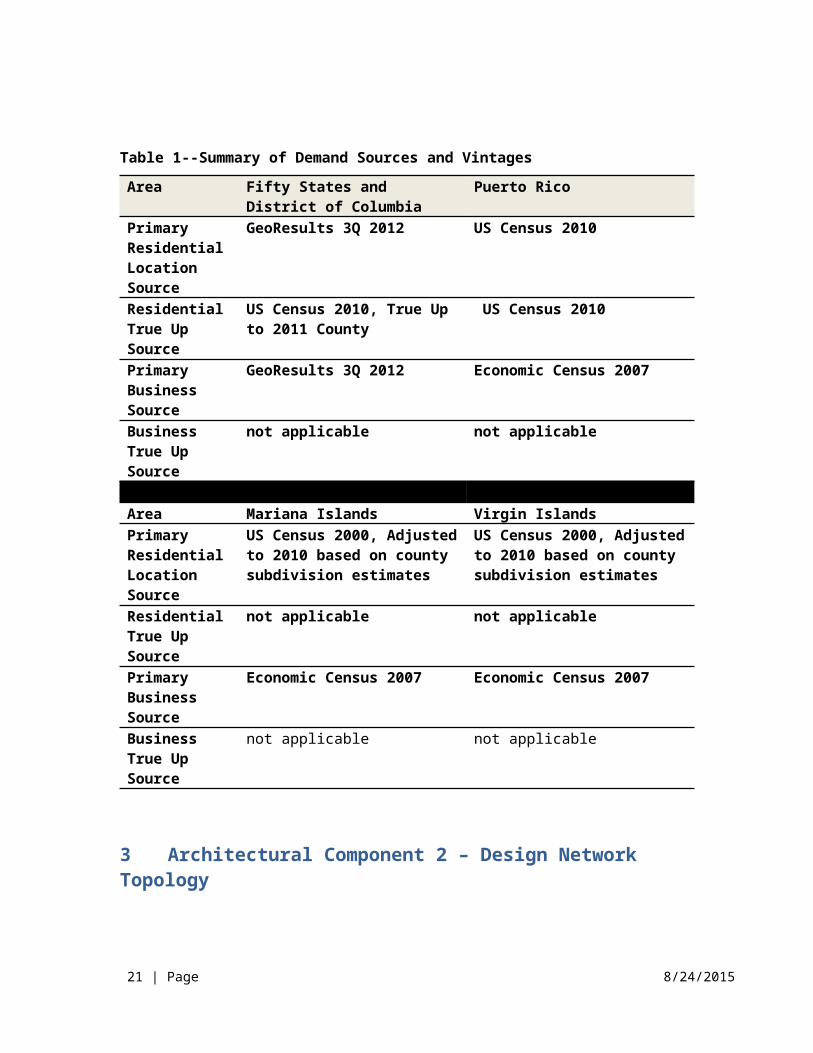
The table below summarizes the different sources and vintages of demand used in the CACM model.
16 | Page 8/24/2015

Table 1--Summary of Demand Sources and VintagesArea Fifty States and District of
ColumbiaPuerto Rico
Primary Residential Location Source
GeoResults 3Q 2012 US Census 2010
Residential True Up Source
US Census 2010, True Up to 2011 County
US Census 2010
Primary Business Source
GeoResults 3Q 2012 Economic Census 2007
Business True Up Source
not applicable not applicable
Area Mariana Islands Virgin IslandsPrimary Residential Location Source
US Census 2000, Adjusted to 2010 based on county subdivision estimates
US Census 2000, Adjusted to 2010 based on county subdivision estimates
Residential True Up Source
not applicable not applicable
Primary Business Source
Economic Census 2007 Economic Census 2007
Business True Up Source
not applicable not applicable
3 Architectural Component 2 – Design Network Topology
3.1. Introduction
Network cost (and hence, any required Support) is a function of network design. CACM’s network design process is initially informed by an understanding of the demand as determined in CACM’s Component 1. In designing a network topology CACM makes use of CostQuest LandLine (CQLL). Additional detailed information on CQLL and its supporting CostQuest Middle Mile (CQMM) model is available in Appendix 1 and Appendix 2, respectively.
3.2. Overview of Approach
CQLL takes Component 1 demand data consisting of approximately 130 million point located records and using real-world network engineering rules, equipment capacities and spatial realities (road systems and relevant terrain
17 | Page 8/24/2015

attributes) assembles / designs an efficient forward-looking wireline network. CQLL is a spatial model in that it connects demand data back to known Central Office locations. It measures media (copper cable or fiber optic cable) along actual road paths and accounts for differences in terrain and demand density. The endpoint of CQLL is a database of network equipment locations and routing required to support voice and broadband-capable networks at a Census Block18 or smaller geographic level.
Where CQLL develops a wireline network from the demand point back to the Central Office, CQMM develops the network middle mile topologies between each Central Office in a state to a location where Internet peering can occur. As noted above, additional information on CQMM is available in Appendix 2.
When users create a Solution Set using CACM’s Fiber to the Premise (FTTp) network topology, they are loading both CQLL and CQMM derived databases into CACM.19
4 Architectural Component 3 – Compute Costs and Develop Solution Sets
4.1. Introduction
The function of CACM’s third architectural component is to determine network deployment (e.g., construction) and operational costs and to establish custom Solution Sets as warranted by user inputs and system default values.
As noted above, at the heart of this component is the Cost to Serve Module – a systematized procedure that takes as inputs geographic and non-geographic data and produces an estimate of the cost of providing voice and broadband capable networks. That is, the Cost to Serve Module estimates the cost to deploy and operate the Network Topology defined by the second CACM component. As such, the Cost to Serve Module provides unitized measures of costs for comparison among Census Blocks.
18 In Census 2010, there are approximately 11 million census blocks. These census blocks are not always coincident with the serving areas of broadband providers. If only part of a block is served by a provider, each provider’s total costs and cost per location will be calculated independently. Similarly, if a block is served by multiple service areas, the cost associated with each service area will be calculated separately. Finally, if a block is served by more than one splitter (Node2), the cost will be calculated separately19 Earlier versions of CACM provided a Fiber to the DSLAM (FTTd) in addition to a Fiber to the Premise (FTTp) topology. 18 | Page 8/24/2015

Output from the Cost to Serve module (and related coverage data) is referred to as a Solution Set. As discussed later in this Methodology, Solution Sets are used in the Support Module to evaluate support and generate reports.
Based on relevant demographic, geographic, and infrastructure characteristics associated within each identified service area – as well as the service quality levels required by voice and broadband-capable networks – an estimate of (a) build-out investments (Capex sub-module) and (b) associated operating costs (Opex sub-module) are developed for each Census Block.
A key input to the second architectural component generally and the Cost to Serve Module specifically is the Network Design. The Network Design provided by CACM’s second architectural component can be thought of as the network schematic. As such it represents a modeled network which is “built” according to real-world engineering rules and constraints. As equipment and cable types and sizes are determined from the network schematic and as unit costs (and related costs) are applied, network costs are computed. These network costs include all the costs associated with the construction of the plant, including engineering, material, construction labor, and plant loadings. The resulting costs are driven to the Census Block level based upon cost-causative drivers.
In the current CACM version a voice and broadband-capable Network Design is available.20
Fiber to the Premise – a design where the entire network from the Central Office to the demand location is entirely fiber optic facilities. In this design, the demand point is within 5,000 feet of the fiber splitter.
In a corresponding component of work within the Cost To Serve module, operating costs (Opex) for service areas are estimated based on certain user-defined criteria (e.g., company size) and certain Census Block-specific profile data (e.g., density). In addition to network driven Opex, operating costs can also be driven by the number of demand locations
In summary, the Cost to Serve Module develops both capital expenditures (Capex Sub-Module) and operating expenditures (Opex Sub-Module) appropriate for the network topology selected.
4.2. Capital Expenditure (Capex) Sub-Module
4.2.1 Build Assumptions and Attributes
20 Previous versions also provided users with the option of selecting a fiber to the DSLAM design. Specifically, CACM’s FTTd option represented a blended copper and fiber design loop consisting of up to 12,000 feet of copper to the DSLAM and fiber from the DSLAM back to the Central Office.19 | Page 8/24/2015

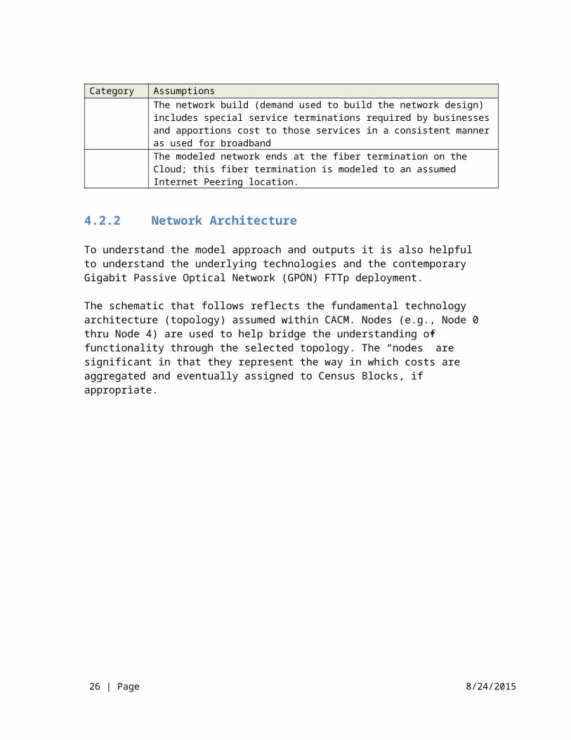
A key to any cost model approach is defining the architectural assumptions and design criteria used to construct the network. The following table summarizes key assumptions and design attributes:Table 2Category AssumptionsOverall Design
Scorched node
Forward-lookingNew network built to all locations All service locations have access to voice and broadband-capable networksContemporary / real-world wireline systems engineering standards are used for the modeling of the network. More specifically, industry standard engineering practices are used for wireline deployments. Long-standing capacity costing techniques are used to apportion investments reflecting real-world engineering capacity exhaust dynamics down to the Census Block level.Network design is based on deployment from known/existing LEC Central Offices (based upon GeoResults Central Office locations).The current service providers continue to supply the service area.Smaller companies have the opportunity to join purchasing agreements with other small companies, improving scale economies.
Coverage Cable broadband coverage currently based on FCC Form 477 (December 2014) data.Wireless broadband (fixed) coverage currently based FCC Form 477 (December 2014) data,
Network Provides broadband-capable networks capable of providing voice and data servicesVoice services provided via cVoIP platform. No Time Division Multiplexing (TDM) investments are presentNo Video equipment (including Set Top Boxes) are installedNetwork is built to a steady state, and results represent a steady state valuation.Plant mix will be specific to each state and can be adjusted as part of an Input Collection.Apportionment of structure, copper, fiber, and electronics will be based on active terminations. For example, working pairs, fibers per DSLAM, etc.The network build (demand used to build the network design) includes special service terminations required by businesses and apportions cost to those services in a consistent manner as used for broadbandThe modeled network ends at the fiber termination on the Cloud; this fiber termination is modeled to an assumed Internet Peering location.
4.2.2 Network Architecture
To understand the model approach and outputs it is also helpful to understand the underlying technologies and the contemporary Gigabit Passive Optical Network (GPON) FTTp deployment.
20 | Page 8/24/2015
The schematic that follows reflects the fundamental technology architecture (topology) assumed within CACM. Nodes (e.g., Node 0 thru Node 4) are used to help bridge the understanding of functionality through the selected topology. The “nodes” are significant in that they represent the way in which costs are aggregated and eventually assigned to Census Blocks, if appropriate.
Figure 3-- Fiber to the Premise Architecture
4.2.3 Network Capital Requirement Development
The Capex Sub-Module takes into account demand locations; efficient road pathing; services demanded at or traversing a network node; sizing and sharing of network components resulting from all traffic; and capacity and component exhaustion from the Network Design selected when a Solution Set is created.
The Cost to Serve module develops unit costs, based upon capacity costing techniques. Unit costs address plant, structure, and electronics to support the voice (cVoIP) and broadband- capable network data requirements of the designed network.
21 | Page 8/24/2015

The voice and broadband-capable network is broken into two key components: loop and middle mile. Additional information on how each component was modeled is provided in Appendices 1 and 2.
The loop portion captures the routing of network facilities from the demand location up to a serving Central Office. This routing captures both the “last mile” (facilities from the demand location to the serving Node2) and the “second mile” (facilities from the Node2 to the Central Office).
The middle mile portion captures what one might typically refer to as the interoffice network or transport. It captures the routing from a Central Office to the point at which traffic is passed to “the cloud.” Within CACM, the connection to the Cloud occurs at a regional tandem (RT) location within a state21.
The following discussion provides an overview of how the two components of the voice and broadband-capable network are developed.
4.2.3.1 The LoopCACM employs CostQuest Associates’ industry recognized CQLL Economic Network model platform to design the network. That is, CACM accepts as inputs network topologies produced by components of CQLL. These files include the distribution (last mile) and feeder topologies (second mile) of the wireline network. The CQLL methodology is discussed in further detail in Appendix 1 to this document.
At a high level, CQLL is a modern “spatial” model that identifies where demand locations exist and “lays” cable along the appropriate (most efficient path) roads of a service area. As a result, a cable path that follows the actual roads in the area can literally be traced from each demand location to the serving Central Office.
From the output of CQLL, a network topology is built that captures the equipment locations and routing required for delivery of voice and broadband services to an entire service area. Within the CACM Capex logic, the network topology is sized to determine appropriate cable and equipment and then combined with equipment prices, labor rates, contractor costs, and key engineering parameters (e.g., equipment capacities appropriate for demand) to arrive at the investments required.
The Capex Sub-Module uses the Network Topology as the basis for a logical economic scorched node build given the technical parameters required for a voice and broadband-capable network.
21 For areas outside of the contiguous United States, CACM uses undersea cable to transport data from non-contiguous areas to the contiguous United States. This is discussed in section 4.2.3.6 and Appendix 2.
22 | Page 8/24/2015
4.2.3.2 CQLL Service AssignmentIncumbent wireline carriers often have an obligation to provision new service within a short period of time. As such, significant components of wireline networks are engineered to meet residential and business service demand within a serving area in recognition of this obligation. That is, certain components of wireline networks are typically built and sized to serve all locations. Service location data are, therefore, key drivers of the network build and instrumental to reliability of the results. The Cost to Serve Module generally and the Capex Sub-Module specifically recognize this operational reality.
As noted above, CQLL is populated with data that incorporate various types of business locations in addition to Census-trued residential locations. Based on this location data set, CQLL then created the network topology required as well as their corresponding service requirements.
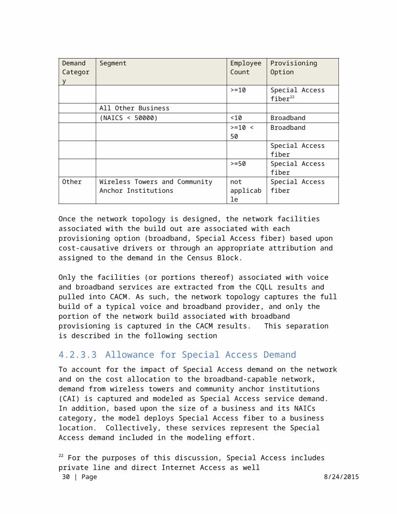
The following table outlines the provisioning option for each category of demand:
Table 3Demand Category
Segment Employee Count
Provisioning Option
Residential
not applicable not applicable
Broadband
Business Technology Oriented Business (NAICS code>50000)
<10 Broadband
>=10 Special Access fiber22
All Other Business (NAICS < 50000) <10 Broadband
>=10 < 50
Broadband
Special Access fiber>=50 Special Access fiber
Other Wireless Towers and Community Anchor Institutions
not applicable
Special Access fiber
Once the network topology is designed, the network facilities associated with the build out are associated with each provisioning option (broadband, Special Access fiber) based upon cost-causative drivers or through an appropriate attribution and assigned to the demand in the Census Block.
22 For the purposes of this discussion, Special Access includes private line and direct Internet Access as well23 | Page 8/24/2015
Only the facilities (or portions thereof) associated with voice and broadband services are extracted from the CQLL results and pulled into CACM. As such, the network topology captures the full build of a typical voice and broadband provider, and only the portion of the network build associated with broadband provisioning is captured in the CACM results. This separation is described in the following section
4.2.3.3 Allowance for Special Access Demand To account for the impact of Special Access demand on the network and on the cost allocation to the broadband-capable network, demand from wireless towers and community anchor institutions (CAI) is captured and modeled as Special Access service demand. In addition, based upon the size of a business and its NAICs category, the model deploys Special Access fiber to a business location. Collectively, these services represent the Special Access demand included in the modeling effort.
The additional fiber which comes from the CAI / Towers or business locations are used in concert with the previously noted demand data to size the total network. The cost of the total network is then attributed to the services based on capacity drivers (e.g., fiber strands, etc.). The cost driven by the fiber strands for these Special Access services are excluded in the cost to serve calculations in CACM. In other words, costs are shared where structure and fiber is shared between the broadband and the Special Access networks. If structure and media are dedicated solely to the Special Access demand, that cost is excluded from the cost to serve calculations. In addition to the exclusion of the cost associated with the Special Access locations, when unitizing total cost in a block within CACM, these Special Access location counts are not used.
For the middle mile portion of the network, a user adjustable percentage of the cost for fiber and structure is assumed for the transport of Special Access demand. In other words, only a portion of the middle mile fiber cable and structure investment is assumed to be driven by the cVoIP and broadband network.
4.2.3.4 Voice CostsCACM supports voice capabilities along with the broadband network. Voice services are provided using carrier grade Voice over Internet Protocol (cVoIP).
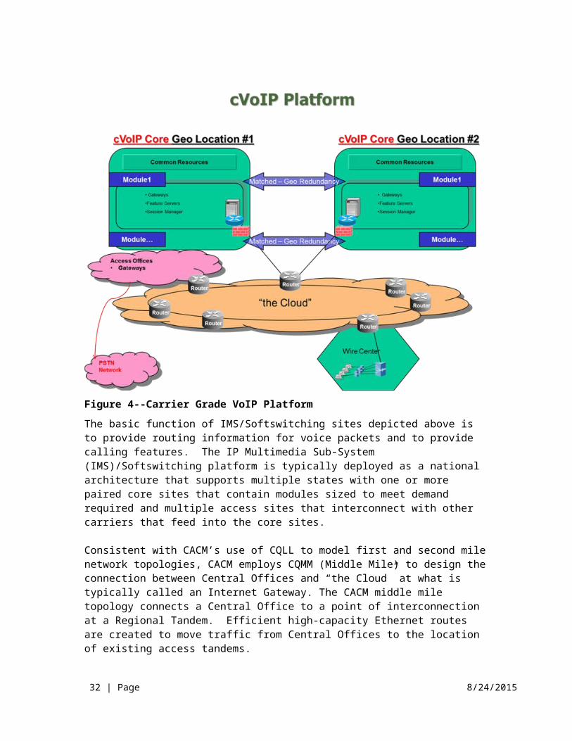
Investments to support voice capabilities are presented to the model on a per unit of demand basis. The typical cVoIP network consists of the following components. For modeling purposes the functionality presented in the following figure is categorized into hardware, software and service categories.
24 | Page 8/24/2015

Figure 4--Carrier Grade VoIP PlatformThe basic function of IMS/Softswitching sites depicted above is to provide routing information for voice packets and to provide calling features. The IP Multimedia Sub-System (IMS)/Softswitching platform is typically deployed as a national architecture that supports multiple states with one or more paired core sites that contain modules sized to meet demand required and multiple access sites that interconnect with other carriers that feed into the core sites.
Consistent with CACM’s use of CQLL to model first and second mile network topologies, CACM employs CQMM (Middle Mile) to design the connection between Central Offices and “the Cloud” at what is typically called an Internet Gateway. The CACM middle mile topology connects a Central Office to a point of interconnection at a Regional Tandem. Efficient high-capacity Ethernet routes are created to move traffic from Central Offices to the location of existing access tandems.
4.2.3.5 Outside Plant Engineering RulesWithin the Capex workbook, CACM provides several rules through which Outside Plant modeling can be modified.
25 | Page 8/24/2015
Typical manhole sizing can be modified in Urban, Suburban and Rural areas with 3 distinct rules:
1. TypicalManholeSizeInUndergroundSystemRural2. TypicalManholeSizeInUndergroundSystemSuburban3. TypicalManholeSizeInUndergroundSystemUrban.
CACM supports placing buried plant in conduit. The percentage of buried placements is an input controlled within the PlantMixBuriedConduit workbook. As an example, a value of 100% in the PlantMixBuriedConduit workbook implies that 100% of buried placements will be buried within conduit. Buried excavation costs are used. Two additional toggles are available to provide additional control.
1. TypicalManholeSizeInBuriedSystem: This toggle allows the user to specify a size1 manhole or to exclude manholes. The exclusion of manholes is the current default.
2. IsInnerDuctUsedForBuriedSystem: This toggle selects the type of conduit used for the buried trench. Currently a duct without innerduct is the default.
Buried trenching costs can be used for underground systems; this logic is turned off by default (UsedBuriedTrenchingCostsForUndergroundSystems = “No”).
Pole logic and investment calculation can be controlled with a variety of rules.
1. PoleSizeWithSharing specifies the height of a pole to use. 2. TypicalGuySpan specifies the distance between guy placements. 3. GuyLengthToPoleHeightRatio provides a ratio to determine guy length
given the pole sizing. The specified value is multiplied by the PoleSizeWithSharing to develop an average guy length.
4. TypicalAerialSpan is meant to capture the average length of a planned aerial span. This is used to calculate the total count of poles needed on a run, assuming 1 is needed at the beginning and end. So if a span is 1200, the typical spacing is 150ft (Pole Spacing table), CACM will place 9 poles (not 8).
5. TypicalCableSegmentLength is meant to capture the average length of a planned build, irrespective of the plant type. This is used to capture Telco Administration/Inspection costs on a per foot basis.
4.2.3.6 Middle MileThe CACM middle mile network connects a Central Office to other Central Offices. It also connects Central Offices to an Internet Gateway.
The approach used to determine the middle mile equipment required – and then to compute the related investment costs – is centered in the spatial relationship between the Central Office and the nearest access to a Tier 3 26 | Page 8/24/2015

Internet Gateway tandem. A surrogate for such access is assumed to be on a Regional access Tandem (RT) ring within the state.
This approach starts with obtaining the location of each Central Office – also referred to as Point of Interconnection (“POIs”) and/or Node0 – from the GeoResults Central Office database. The result of this approach aligns the Central Office/Node0 locations used in the underlying CQLL model’s network for the local loop.
Regional tandem locations (and the relevant feature groups deployed) are obtained from the LERG ®database. Each tandem identified as providing Feature Group D access in LERG ® 7 is designated an RT. As with Central Offices, a latitude and longitude is identified for each RT.
The underlying logic (and the process) of developing middle mile investment requirements are grounded in the assumption that the Internet Gateway peering point is located on the RT ring – meaning that if the modeled design ensures each Central Office is connected to an RT ring, the corresponding Node0 demand has access to the Internet.
For areas outside of the contiguous United States, undersea cable and landing stations support links between the RT and the contiguous United States. Within non-contiguous areas, submarine cable and beach manholes are used to support middle mile routes that intersect water bodies (e.g. routes going from one island to another island). Additional information on undersea and submarine modeling can be found in sections 8.2 and 8.4 of this document.
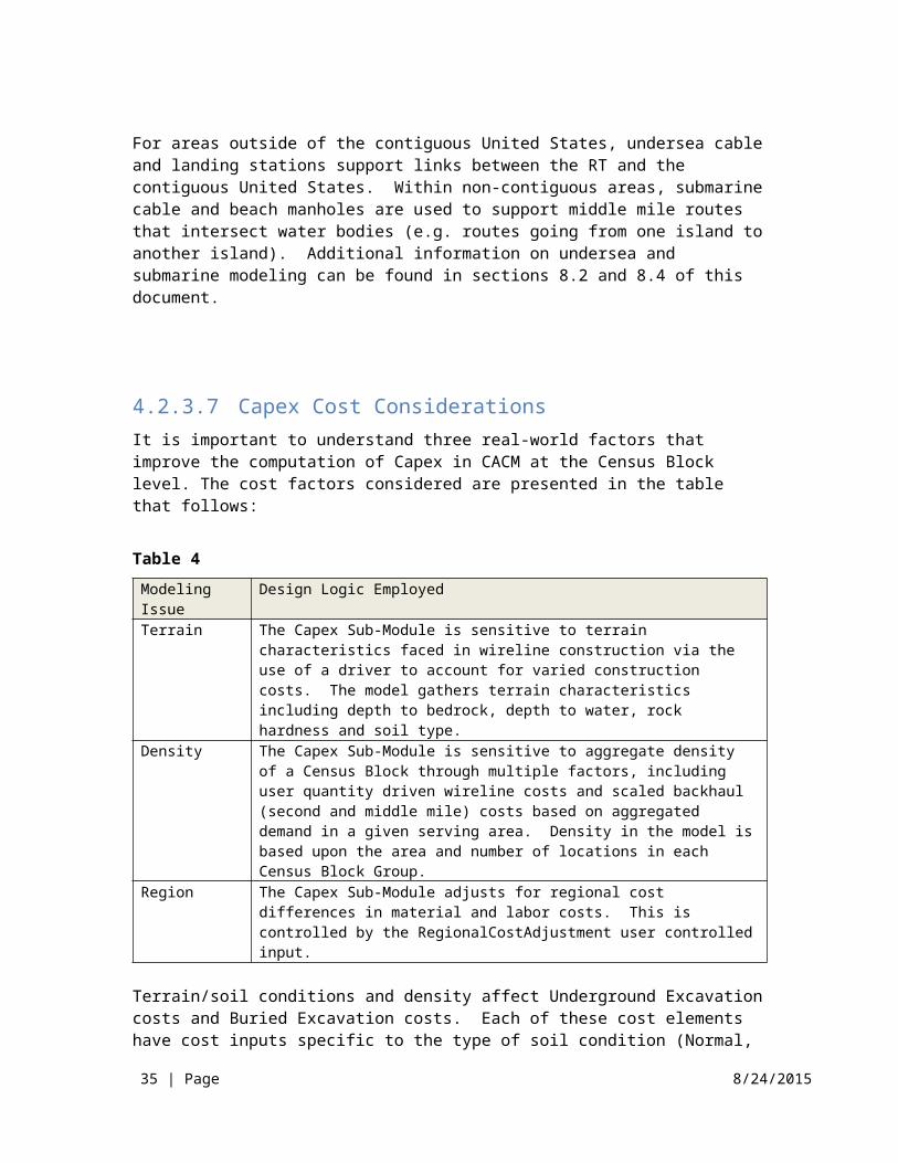
4.2.3.7 Capex Cost ConsiderationsIt is important to understand three real-world factors that improve the computation of Capex in CACM at the Census Block level. The cost factors considered are presented in the table that follows:
Table 4Modeling Issue
Design Logic Employed
Terrain The Capex Sub-Module is sensitive to terrain characteristics faced in wireline construction via the use of a driver to account for varied construction costs. The model gathers terrain characteristics including depth to bedrock, depth to water, rock hardness and soil type.
27 | Page 8/24/2015
Modeling Issue
Design Logic Employed
Density The Capex Sub-Module is sensitive to aggregate density of a Census Block through multiple factors, including user quantity driven wireline costs and scaled backhaul (second and middle mile) costs based on aggregated demand in a given serving area. Density in the model is based upon the area and number of locations in each Census Block Group.
Region The Capex Sub-Module adjusts for regional cost differences in material and labor costs. This is controlled by the RegionalCostAdjustment user controlled input.
Terrain/soil conditions and density affect Underground Excavation costs and Buried Excavation costs. Each of these cost elements have cost inputs specific to the type of soil condition (Normal, Soft Rock, Hard Rock or Water (i.e., high water table) and the density of the area. Based upon soil/terrain and density information associated with each plant element, the model uses the relevant associated Capex cost input to estimate the cost of structure placement in the specific soil type and density in which the structure is being placed. In other words, as an output of the Network Design each plant element has an associated terrain and density attribute. Based upon the terrain attribute, the appropriate investment lookup is made.
4.2.3.8 Terrain Factor DevelopmentTo support cost sensitivity driven by terrain factors, a terrain by Census Block Group (CBG) table was developed.
For the contiguous states, Puerto Rico and Alaska, the terrain by CBG table was sourced from Natural Resources Conservation Service (NRCS) STATSGO data.23
For VI and MP, SSURSGO data was used.
In both cases, the following attributes were used:
Bedrock Depth Rock Hardness Water Depth Surface Texture
The Bedrock and Water Depth for each Census Block Group represented the area weighted average of each STATSGO/SSURGO Component Map Unit relative to the Census Block Group. The Rock Hardness used was the most frequently occurring value. When developing the Terrain by CBG table, the STATSGO Component polygons had to cover at least 20% of the Census Block Group to be represented in the calculations. For the contiguous United
23 Data extracted from, http://soildatamart.nrcs.usda.gov/. Website deactivated 4/24/2013.
28 | Page 8/24/2015

States, where no STATSGO or SSURGO data elements covered at least 20% of the CBG, values were filled as NULLS.
In Alaska, Puerto Rico and Hawaii, terrain assignments to Census Block Groups (CBGs) were made such that any CBG with at least 50% of the area covered by a STATSGO component polygon with a RockHardness value of Hard was assigned a RockHardness value of Hard.
Based upon the depth to bedrock, water and the rock hardness assignments to Hard, Soft, Normal and Water terrain types were made. With these assignments made on each plant element, appropriate terrain driven inputs are applied by CACM.
4.2.3.9 Density DevelopmentSince CACM version 2, density is measured at the Census Block Group level and based upon the sum of locations in the Census Block Group divided by the area of the Census Block Group. The resulting numerical value is then translated into Urban (equal to and above 5000/sq mi.), Suburban (equal to and above 200/sq mi.) and Rural.
4.3. Operational Expense (Opex) Sub-Module
The CACM Opex Sub-Module estimates wireline telecommunication operating expenses incurred in provisioning voice and broadband in service areas by company size and by density. The CACM Opex Sub-Module is applied to Census Block profiles with consideration of coverage requirements defined by a set of user assumptions and investments.
The CACM Opex cost profiles are presented within a hierarchy of costs referred to as the CostFACE. From the highest level in the hierarchy down, the CostFACE is comprised of the following:
F – Cost FAMILY (e.g., Network vs. Customer Operations vs. General and Administrative)A – Cost AREA (e.g., Plant Specific vs. Plant Non-Specific)C – Cost CENTER (e.g., Cable & Wire vs. Circuit Equipment vs. Switching)E – Cost ELEMENT (e.g., Copper Aerial v. Fiber Aerial v. Copper Buried v. Fiber Buried)
The purpose of the CostFACE is to organize and align operating costs with relevant cost drivers (e.g., associated Capex investment and demand24).
24 The term demand is used to reference connected and non-connected locations on the network. In the past subscribers was used synonymously (to represent all network demand locations) but some readers were confused by that reference. Therefore, demand is used in this document to represent both connected and non-connected locations.29 | Page 8/24/2015
The model input is organized in a set of static tables made available to CACM for purposes of aligning the selected operating costs to the selected provider type, size, and density based on cost drivers, such as investment or service locations.
To provide estimated operating expense for the difference in operating characteristics noted above, relevant provider data available within the public domain were gathered and analyzed to develop a set of baseline cost profiles and a corresponding set of factors or cost functions designed to adjust the baseline views by provider size and density. These publicly available values were then validated against proprietary data provided by ABC Coalition members.
The steps in the operational cost development process vary by provider size, but are summarized generally below:
Research and gather operating expense data; Segmentation of data into uniform expense lines; Analysis of data; Identification of appropriate CACM Opex Sub-Module cost drivers
based on best available data; Development of baseline Opex detail; Development of factors for size and density adjustments; Development of property tax location adjustments; and Validation and revalidation of results.
4.3.1 Opex Assumptions
Developing a forward-looking cost model which includes operational expense functions is complex. What you are trying to do is develop a forward-looking Opex value for a network which may not yet be in place over the assumed geographic scope of the network.
To accomplish this, existing data sources must be examined, potentially comingled and compared across a number of dimensions to yield a relevant estimate of Opex.
There is no existing readily available source for detailed cost by technology by operating cost category, by geographic area, by density which is aligned with accessible cost drivers. This is the type of information that is needed in a forward-looking modeling effort. Rather, there are a limited number of relevant data points found across an array of information sources. This implies that developing data sources which are inputs into CACM processing will be complex. The quality standard by which the CACM inputs were evaluated was their consistency among company sizes, consistency with prior forward-looking results, and comparability to proprietary data sources, if those sources are available.
30 | Page 8/24/2015
The process to develop the CACM inputs to the Opex sub-module relies on certain assumptions and limitations that constrain the absolute predictability of the Opex Sub-Module, as listed below:
a) Industry-reported financial data are reasonably accurate and sufficiently segregated to develop Opex drivers to model operating expenses at geographic granular levels (i.e., Census Blocks);
b) Varying formats and expense-detail levels of publicly available financial data can be reconciled to provide compatible detail;
c) Compilation of publicly available information can be analyzed using regression equations, averages, and other acceptable analysis derived from industry information to derive baseline Opex detail;
d) Resulting unitized baseline expense detail can be modeled against CACM forward-looking cost drivers to approximate reasonable estimates of Opex for selected provider, size, and density characteristics;
e) Historic financial data comprised of mixed technological generations can be adjusted to predict the operating expense of deployed new technology; and
f) Varying types of expense detail can be validated against industry or company-specific data.
4.3.2 Sources of Information
The following information sources were the primary sources from which the Opex data were derived, analyzed, and tested/validated:
FCC ARMIS Datao Pulled from: FCC Report 43-01 for 2007 and 2010
NECA Datao Pulled from: http://transition.fcc.gov/wcb/iatd/neca.html for
2006-2010 Section: “Universal Service Fund Data: NECA Study
Results” Thomson Reuters’ Checkpoint/RIA Wolters Kluwer’s CCH (Commerce Clearing House) Comments filed in National Broadband Plan docket Telecommunication Carriers Public Financial Statements 2009-2010 Standard & Poor’s Industry Surveys: Telecommunications: Wireline,
April 2011 Business Monitor International, United States Telecommunications
Report, Q1 2011 Morgan Stanley, The Mobile Internet Report, December 15, 2009 R.S. Means, Building Construction Cost Data 69th Annual Edition
(Massachusetts: R.S. Means Company, Inc. 2010)31 | Page 8/24/2015
Marshall & Swift, Marshall Valuation Services (U.S.A.: Marshall & Swift/Boeckh, LLC, 2010)
Certain proprietary and third party information, including data provided by the ABC Coalition
Additional information regarding Opex development is available as a presentation posted to the Resources section of the CACM website-- Opex Overview.zip.
4.3.3 Development of Opex Factors
The sections that follow provide an overview of the methodology used to develop the CACM Opex Sub-Module factors and related adjustment factors for the various FACE elements.
The table immediately below shows the detail operating cost functions that are represented in each level of the CACM FACE.Table 5
FACE Primary Level Second Level Third Level
Network Operations Expense Plant Specific Outside Plant Cable by Cable
Type Poles Conduit Circuit / Transport
Plant Non-Specific Network Operating Expense
General Support and Network Support
General and Administrative n.a. n.a.Selling and Marketing n.a. n.a.Bad Debt n.a. n.a.
4.3.3.1 Network Operations Expense FactorsTo estimate the CACM Network Operations Expenses, the relationship between capital investment and ongoing cost to operate and maintain the plant was determined.
This determination relied primarily on three years of NECA data (2008-2010), supplemented with additional data sourced from ARMIS and third party sources25. These NECA data report operating expenses, Investment by Plant Type in Service (IPTS), and Total Plant in Service (TPIS) amounts for
25 These third party sources include material provided by the ABC Coalition companies.32 | Page 8/24/2015
companies across common USOA Part 32 accounting categories CO Transmission and Circuit Equipment, and Cable & Wire accounts.
These data were further categorized with a size variable using the NECA reported line counts.
A NECA rural classification was overlaid on the company size data. In addition, the cable and wire accounts were broken out into Aerial Cable, Buried Cable, Conduit, Poles, and Underground Cable using industry data percentages of distribution plant (e.g., Opex & Plant Investment) pulled from ARMIS.
Finally, the data were unitized on a per-loop basis to facilitate the validation/testing of the results by company size and density.
Development of the network operations expense investment-based factors relied on NECA data (2008-2010), segregated by company size and density. Two analytic paths were investigated. The first was a regression analysis to develop Opex regression coefficients. The second was a mean analysis to develop the median and average Opex / IPTS factors per loop. The mean analysis was used.
The median and average operating expense to plant investment per loop were determined and were then averaged to derive the NECA-based Opex to Plant Investment factor.
These results were then adjusted from a historical cost basis to a contemporary topology-specific network build on a forward-looking cost (“FLC”) basis, resulting in the baseline CACM Opex Sub-Module factors. Once model output was available, the scaling was revisited to ensure that forward-looking opex values did not exceed NECA-based Booked Opex that were derived by applying the initial NECA-based Opex to Plant Investment Factor to the weighted average NECA-based plant investment per loop which resulted in the annual operating expense per loop by company size and density.
From these data, cable CACM Opex Sub-Module factors were further segregated between metallic and non-metallic to account for the significant operating differences between the two types of cable using proprietary data sources. Finally, a large company baseline view was extracted based on the cost categories discussed in the Cost Face format illustrated above. Factors were then derived to adjust for size, density, and location.26
4.3.3.2 General and Administrative Operating ExpenseTo calculate the CACM General and Administrative (“G&A”) Opex sub-module factors, a regression analysis was employed using five years (2006 - 2010) of 26 The density measure used in CACM (associated with the Census Block Group which the Census block falls within) is used to determine both the appropriate Capex and Opex values for the Census block.33 | Page 8/24/2015

NECA G&A Opex (dependent variable) and Total Plant in Service (“TPIS”) (independent variable) data segregated by company size to determine the relationship between total plant investment and G&A operating expenses. Using the same type of NECA investment data unitized on a per loop basis as used in the network operations analysis, FLC G&A Opex Component factors per loop were developed by company size and by density using a regression equation. Comparing the contemporary G&A Opex Component factors to the regression parameters resulted in a set of FLC to historical G&A adjustment factors by company size and by density. Applying these adjustment factors to the regression parameters resulted in the CACM G&A Opex Component factors by company size by density. The Large Company baseline results were then validated by comparing them to G&A operating expense data provided by the ABC Coalition companies.
4.3.3.3 Customer Operations Marketing & Service Operating ExpensesTo determine the CACM customer selling and marketing (“S&M”) Opex Sub-Module factor, the effort employed publicly available ARMIS data and ABC Coalition company data. Based on the ABC Coalition company data, overall S&M costs were estimated as a percent of total operating revenue. In addition, a review of the latest ARMIS data available for large incumbent local exchange carriers (“ILECs”) (2007) and mid-sized ILECs (2010) indicates S&M operating expenses are 12.97 percent of all ARMIS reported revenue. Both percentages were averaged and applied to the assumed ARPU of the CACM service(s) to derive the CACM S&M monthly operating expense perNode4WorkingCust. Node4WorkingCust represents total locations passed.
An analysis of ARMIS data also indicates that 41 percent of the S&M is attributable to marketing with the remaining 59 percent associated with “Customer Operation Services”.
4.3.3.4 G&A Opex Property Tax Location AdjustmentProperty taxes are typically a subset of the G&A operating expense. Property taxes, which are based on the value of the property owned by the taxpayer in the taxing jurisdiction as of a particular lien date, vary by state and, to some degree, by taxing authority within each state. As such, location-specific property tax indices to be applied to the G&A Opex Component factors were developed.
To develop the location-specific indices, total corporate operations expenses (G&A plus Executive & Planning) and the net plant in service, based on the NECA data, were summarized by state. The effort then developed the average property tax levy rates by state. Applying these levy rates to the net plant in service (e.g., proxy for the taxable property tax value) resulted in the implied property tax expense by state. Comparing these figures to the overall national weighted average property tax levy rate, property tax indices by state were developed. Applying these indices to the G&A operating expense adjusts for location-specific differences in property taxes.
34 | Page 8/24/2015
4.3.3.5 Bad Debt ExpenseThe CACM Bad Debt Module expense is applied on a Node4WorkingCust basis and was estimated based on using a revenue derived bad debt factor and an assumed ARPU. The bad debt factor as a percentage of all reported revenue was based on a review of industry-specific 10K’s and industry knowledge.
4.3.3.6 ValidationThe accuracy of the CACM Network Opex Sub-Module factors was tested by applying them to the estimated CACM Capital Investment Module factors per loop and comparing the results to the NECA network operating expenses per loop by company size and by density.
The CACM operating expense output by cost element also were reviewed for differences in density, technology, and other factors. General and Administrative and Selling & Marketing expenses also were validated against data reflecting the provisioning of cVoIP and broadband services.27
4.3.4 Operational Cost Sub-Module Conclusion
As the Cost to Serve module completes its processing, the model captures the average monthly cost of service for each of the over 11million Census Blocks in the country. This monthly cost includes the monthly operational costs and the capital related monthly cost of depreciation, cost of money and income taxes. These capital costs are developed through the application of levelized annual charge factors applied to the Capex that is developed by the model. As described above, the output of the Cost to Serve module is stored in and referred to as a “Solution Set.” Solution Sets are used by the Support Module along with specific user parameters to calculate a result.
4.4. Cost To Serve Processing Steps
From an implementation perspective, the computation of Architecture Component 3’s Capex and operating costs (Opex) is accomplished in CACM through the steps in Table 6. The steps are described below but processing source code is available to interested users.
27 Output was also compared to confidential, actual data where those data were available. The CACM website contains additional information about Opex development. The Opex Overview presentation describes how the Opex workbook was developed as well as source data used. It is available on the Resources page. The Connect America Phase II Cost Model workshop < http://www.fcc.gov/events/connect-america-phase-ii-cost-model-workshop> also provides additional information.
35 | Page 8/24/2015
The System Evaluator version of CACM (CACM-SE) allows users to view resolved processing code and step through each of these steps viewing calculations, updates to tables and report definition files.Table 6
Step Description Comments
0 Prepare Coverage Prepares coverage table using base coverage, augmented with available coverage and challenge coverage if available for each technology.
1 Initialize Solution Set Creates the Solution Set entity that will frame the computations to follow and hold results when completed.
2 Update CT Density Calculates Census Tract Density to be used in a later calculation.
3 Define distribution network
Establishes the consumer and business demand and related distribution network topology.
4 Estimate demand Develops consumer and business demand based on take rates. 28
5 Determine bandwidth throughput requirements
Develops bandwidth throughput required based on consumer and business demand determined in previous steps
6 Not Used (see Note) 7 Determine Demand at
DSLAM or Fiber SplitterDevelops data important to the sizing of Node2 investments (i.e., at the DSLAM or Fiber Splitter)
8 Create intermediate Capex table
Develops and incorporates defining network cost drivers such as terrain, density, company size and location, tax rates, etc.
9 Develop Capex for distribution and feeder
Updates the Solution Set with investment required for the Distribution network (i.e., from Node0 through Node4)
10 Develop Capex for Middle Mile
Updates the Solution Set with capital investment required for the Middle Mile (i.e., from Node0 to Node00)
11 Develop Investment Related Opex
Updates the Solution Set with investment related Opex and pre-stages the computation of full operating costs
12 Develop Non-Investment Related Opex
Updates the Solution Set with non-investment related Opex including adjustments for regional cost and property tax differences)
13 Populate Solution Set Completes the Solution Set and makes it ready for use in the Support Module
Note Other Comments This table presents the processing code steps as used in the current CACM release. The full system code includes certain steps that are inactive.
5 Architectural Component 4 – Define Existing Coverage
28 CACM receives take rate information from the residential and business take rate tables. These tables are described in Appendix 6. The impact of these take rate inputs on network sizing and unitization is described in Appendix 10.36 | Page 8/24/2015
5.1. Introduction
The function of A-CAM’s fourth component is to inventory existing voice and broadband coverage and associate that coverage with providers and specific geographies. The outcome from this component is a preprocessed coverage database that is derived from FCC Form 477 data and lists of subsidized competitors by Study Area Code (SAC). The coverage database informs A-CAM as to what broadband technology is currently serving a Census block as well as what Maximum Advertised Downstream and Maximum Advertised Upstream speeds are available in that block. The combination of a broadband technology and the speed in which it is available determine if a Census block is served by a particular technology.
5.2. Information Source and Process
Broadband coverage information, specifically the speed and technology available in each Census block, is sourced from FCC Form 477 data (based on December 2014 Form 477 submissions).29 Broadband providers submit Form 477 every six months.
The derivation of the coverage data used in A-CAM started at the Census block level by examining each distinct technology group, maximum advertised downstream and maximum advertised upstream speed record by provider. As described below, technology and provider level filters are applied. These filters included the type of broadband technology used as well as whether the provider reports voice services on FCC Form 477 and if the provider receives a subsidy.
Within this process, the Technology of Transmission codes were used to develop technology groups as follows.
Telco broadband includes Technology of Transmission30 Codes 10, 11, 12, 20, 30 and 50
Fixed Wireless includes Technology of Transmission Codes 70
Cable includes Technology of Transmission Codes 40, 41 and 42
Excluded codes are 60 (satellite), 80 (mobile wireless), 90 (BPL) and other (0).
In summary, broadband coverage for A-CAM was developed in a similar manner to prior releases. Cable and Fixed Wireless coverage was removed if
29 The Form 477 data are preliminary and subject to revision.30The Technology of Transmission Codes for Deployment of Fixed Services are available at Wireline Competition Bureau Releases Data Specification for Form 477 Data Collection, WC Docket No. 11-10, 28 FCC Rcd 12665 (2013), Appendix, Table 1, https://apps.fcc.gov/edocs_public/attachmatch/DA-13-1805A1_Rcd.pdf.37 | Page 8/24/2015

a provider did not report voice services31 and residential broadband32 on FCC Form 477 (December 2014) or if the provider receives a subsidy within a particular Study Area.
Broadband coverage development was based upon information from FCC Form 477, December, 2014. The coverage development process starts by filtering Form 477 coverage data to those providers reporting residential broadband and voice services. If a provider does not indicate they offer both, they fall out of this step and will not show as covered in A-CAM.
Remaining coverage is then examined to remove the coverage of subsidized providers. Subsidized providers are identified from FCC Claims information.33 Only the broadband coverage of the subsidized provider within the supported Study Area is removed.
Once the eligible coverage, technology groups and related downstream and upstream speeds were available in each block (i.e., consumer maximum advertised), a ranking process was developed to determine the available speed by technology by block.
This next step categorized the FCC Form 477 maximum advertised speeds into bands.34 Band labels (e.g., Good, Better, Best) are a function of both download and upload speeds expressed in Mbps. The process starts at the Best category and decrements, examining each Census Block, provider / speed / technology combination, assigning the value to the first rank category judged true.
o Best: Download at or above 10 and upload above 1.5
o Better: Download at or above 10 and upload at or above 1
o Good: Download at or above 3 and upload at or above 0.768
o Poor or Null: Download under 3 and/or upload under 0.768
With the bands of each Census Block identified, the process then picked the top band available within the Census Block. Within the top band, if there is a
31 Voice services are offered by a provider if Local Exchange Telephone or Interconnected VoIP = “X” on the StateFilers1214.xls table. Available at https://www.fcc.gov/encyclopedia/form-477-filers-state-32 Residential broadband is defined as Consumer=1 within the FCC Form 477 Fixed Broadband Deployment table.33See, https://www.fcc.gov/encyclopedia/federal-state-joint-board-monitoring-reports. Select “Updated 2014 High-Cost Claims” under 2014 Monitoring Reports.34 A coverage record represents a single carrier’s technology of transmission and maximum advertised consumer speed within a Census Block.38 | Page 8/24/2015

tie, the process picks the best available speed, using the record with the superior upload speed.
The resulting ranked speed assignment by technology group by Census Block is then imported into the CACM Solution Set. The resulting broadband speeds by Census Block and technology group are compared to the appropriate threshold to determine if a Census Block is served or unserved.
6 Architectural Component 5 – Calculate Support and Report
The function of CACM’s fifth and final component is to allow users to compare support options, view final model results and review / audit model detail. Sometimes referred to as the “Support Module” this component includes a mathematical procedure that takes cost output (Solution Set) data from the Cost to Serve module as an input and produces a universal service support amount based upon parameters set / entered by the user.
Once the Cost to Serve Module has run, a large amount of information is available for analysis and decision making. As described earlier, the Support Module takes the output (Solution Set) from the Cost to Serve Module along with user-defined parameters to calculate a result representing universal service support specific to the user request. The Support Module examines the granular cost information and calculates those areas requiring support given a specific set of parameters.
6.1. Factors that Determine Support
A few of the critical considerations in determining high-cost universal service support amounts and included in the Support Module are:
geographic unit for calculating costs and support; eligible blocks for funding based upon the presence of an alternative
voice and broadband provider, funding benchmark above which areas are eligible for support; extremely high cost threshold above which areas are not eligible for
support, which may be better served by an alternative technology; and
overall funding budget (CAF II Funding Budget)
Once the user selects the appropriate support attributes and associated values, CACM reporting will provide a summary of the funding requirements based on the user’s selections. By default, CACM reporting will remove census blocks served by fixed wireless and cable broadband providers from
39 | Page 8/24/2015

support eligibility (with the Cable and Fixed Wireless Unserved set to “True”)35, unitize costs to No TakeRate Demand (unitizing costs by locations passed) and filters output to only Rate of Return carriers. Results can be rolled up to multiple Geographic Levels.
6.2. CACM User Controlled Reporting Parameters and Output Descriptions
The following terms are used on the Support Module interface. Cost and Total Funding amounts specified are in dollars per month, unless noted otherwise. Definitions are provided below.
Target Benchmark - The cost benchmark to which a candidate area’s per unit cost is compared to determine where funding is required. Locations with unitized cost below the Target Benchmark are excluded from the support calculation, and the value of the Target Benchmark is deducted from the support amount for locations with unitized cost above the Target Benchmark. The Target Benchmark is also referred to as a funding benchmark or benchmark.
Alternative Technology Cutoff – The input value representing the support limit or alternatively the cost increase over the Target Benchmark36. If the candidate area’s unitized cost is greater than the funding benchmark plus the Alternative Technology Cutoff, the number of service locations in the candidate area is excluded from support and designated as an extremely high cost location.
Cable Unserved – Used to include or exclude cable served areas in the analysis. Setting this value to false will allow Cable Served blocks to be eligible for support.
Fixed Wireless Unserved – Used to include or exclude fixed wireless served areas in the analysis. Setting this value to false will allow Fixed Wireless Served blocks to be eligible for support.
Rate of Return/Price Cap – A parameter used to show either Rate or Return (ROR), Price Cap (PC) or both provider types simultaneously in a given report. Average Schedule and Rate of Return affiliates of Price Cap companies are treated as Price Cap in this filter.
Unitize Cost By – A toggle used to determine how cost is unitized. Total Cost can be unitized by either a take rate impacted demand (sometimes
35 As noted above, currently there is no difference in the user interface or processing logic of CACM/CAM and A-CAM. See supra note 3. In CACM 4.2 the census blocks served by fixed wireless and cable broadband include both unsubsidized competitors and subsidized competitors. See December 2014 Connect America Order, FCC 14-190 at paras. 73-74 & n.169.]]36 The funding benchmark plus the Alternative Technology Cutoff is referred to as the extremely high cost threshold.40 | Page 8/24/2015

described as connected locations) or non-take rate impacted demand (sometimes described as locations).
Reports also may be produced for different levels of geography. This field only specifies the manner in which the data in the report are presented, and does not change the granularity of calculations. That is, CACM computations are done at the Census Block level while CACM reports are available at a higher/summarized level. These areas are explained below.
Census Designated Place – A geographic entity that serves as the statistical counterpart of an incorporated place for the purpose of presenting census data.
Census Block Group – A Census Block group (CBG) is a cluster of Census Blocks having the same first digit of their four-digit identifying numbers within a census tract.
Census Tract – A census tract represents a relatively permanent statistical subdivision of a County.
Company – An abbreviation of the name corresponding to the 14 largest (by line count) telephone providers. If not named, designated as small (SML)
County – The primary legal divisions of most states are termed counties. If a state or territory doesn’t have counties, the statistical equivalent area (e.g. Borough, Parrish) is used.
OCN – Operating Company Number based upon GeoResults 2012, 4Q as revised with assistance from FCC, USAC and responses to public notice.
SAC – Study Area Code identifying a collection of Study Areas as described by the Universal Service Administrative Company (USAC).
Serving Area – An area, based on GeoResults, corresponding to the serving wire center boundary of an incumbent LEC.
State – State provides a geographic rollup where State is defined as the 5th and 6th character of the service area.
6.3. Support Model Report Output Field Definitions
The following table describes the calculation for each of the output columns related to the Support Model reports.
As described in Appendix 10, the reported values for some fields in this table, such as Cumulative Percentage of Subscribers at Rollup, are impacted by the unitization toggle used when the report is defined.
41 | Page 8/24/2015
On export to CSV (comma separated variables), many columns rename to their system definition. Where a calculation is shown in the second column, the definition reflects a pseudo-code explanation. The actual processing code is available within the stored procedures called by the report.
Table 7Report Field Name Definition/Calculation
Benchmark The lower cost threshold at which funding begins.
BMrk_less_Cost_per_Demand_Unit
Target Benchmark minus Monthly Cost Per Demand Unit
Cable Unserved Used to include or exclude cable served areas in the analysis. True excludes served areas.
Company Name An abbreviation for the incumbent provider
County The primary legal divisions of most states are termed counties. If a state or territory doesn’t have counties, the census equivalent
Cumulative Percentage of Subscribers at Rollup
Running total of demand divided by sum of all demand * 100.
Cumulative Total Max Funding
The accumulation of Total Max Funding up to the Total Max Funding (input parameter). In the detail report, once the Total Max Funding hits this value, this Total Max Funding is reported for each detail record thereafter.
DemandUnits Over Alt Tech Cutoff
The sum of Total DemandUnits whose average cost are over the Alterative Technology Cutoff. The model determines which demand is over the Alternative Technology Cutoff by determining if the Benchmark minus Cost Per Unit of Demand is greater than the Alternative Technology Cutoff; then the Active Subscriber is Over the Alt Tech Cutoff, otherwise the demand is under the cutoff.
DemandUnits SprtElgbl Each Census Block record when rolled up to a specified geographic level is determined to be eligible for support based on this calculation. Calculation: If the Total Max Funding > 0 then DemandUnits Under Alternative Technology Cutoff and over Benchmark, otherwise it is 0. This is then summed to get the demand subsidized.
DemandUnits Under Alt Tech Cutoff
The DemandUnits under the Alternative Technology Cutoff. Sum of DemandUnits where Alternative Technology Cutoff is not exceeded.
Monthly Cost Per DemUnit Total Cost / Demand Unit in specified geographic area
42 | Page 8/24/2015

Report Field Name Definition/Calculation
OCN Operating Company Number based upon the GeoResults wire center boundary wire center to OCN association as well as corrections from support tickets and public notice response.
Per Unit Funding Total Max Funding / Demand Units Under Alt Tech Cap
SAC Study Area Code identifying a collection of Study Areas as described by the Universal Service Administrative Company (USAC)
Service Area An area corresponding to the serving boundary of an incumbent telephone provider. The Service area is based upon GeoResults, wirecenter boundaries.
Short Name An abbreviation for selected incumbent providers
State State provides a geographic rollup where State is defined as the 5th and 6th character of the Service area
Support Capped Funding Amount of funding the provider/candidate requires up to the Monthly Support Funding Cap (input parameter37). If the Alternative Technology Cutoff is not exceeded then, Support Capped Funding is 0 when Benchmark-(TotalCost/Unitization Value)* FCC Portion38 *Unitization Value) is larger than or equal to 0. Otherwise it is FCCPortion*(TotalCost/Unitization Value)-Benchmark when (TotalCost/Unitization Value)-Benchmark is less than SupportFundingCap, and FCCPortion*SupportFundingCap when (TotalCost/Unitization Value-Benchmark) is greater than the SupportFundingCap
37 The complete CACM processing code has a provision whereby a user input monthly cap on per unit funding can be set. As this is not how CACM is currently used, this input parameter has been removed. The pseudo-code description used above retains the reference for completeness and consistency with the underlying system code.
38 The complete CACM processing code has a provision whereby a pre-determined Federal portion of an allowable support amount would be determined by the FCC. This functionality is not active in version 3.1 forward. As a result, the “FCCPortion” value in the currently employed code is set to 100%. The pseudo-code description used above retains the “FCCPortion” reference for completeness and consistency with the underlying system code43 | Page 8/24/2015
Report Field Name Definition/Calculation
Telco Served DemandUnits
The number of funded DemandUnits that are broadband served by a Telco. Served refers to having a downstream/upstream speed sufficient to be judged as served. This test is made for an entire Census block. “DemandUnits SprtElgbl” refers to the Demand Units under the Alternative Technology Cutoff'.
Telco Unserved DemandUnits
The number of funded DemandUnits that are not broadband served by Telco. Unserved refers to having a downstream/upstream speed insufficient to be judged as served
Total Cost Sum of Total Cost (Total Opex Cost + Capital Cost) where Alternative Technology Cutoff is not exceeded. Cost is a monthly value
Total DemandUnits This is the sum of demand units over any user entered Benchmark.
Total Investment This is the Total Investment from the Solution Set that is under the Alternative Technology Cutoff. If there is no Alternative Technology Cutoff, then this is the sum of Total Investment from the Solution Set.
Total Max Funding The amount of total funding based on the support module before the application of any support funding caps. A demand unit could have cost in excess of the benchmark, but not get funded, since the available funding was exhausted prior to funding the provider/candidate or a support cap was in place. At the point where the Cumulative Total Max Funding reaches the Total Max Funding (input parameter) the last record is the dollar amount where the funding is exhausted. All detail records after this point will have a value of 0. Total Max Funding is 0 when BMrk_less_Cost_per_Demand_Unit is less than 0 and Cumulative Total Max Funding is less than the Total Max Funding Parameter amount. For all other cases if (Total Max Funding Parameter amount -TotalCappedFunding)/(-1*BMrk_less_Cost_per_Demand_Unit*TotalDemandUnits*FCCPortion) is greater than 1 then Total Max Funding is (Total Max Funding Parameter amount -TotalCappedFunding), and if (Total Max Funding Parameter amount -TotalCappedFunding)/(-1*BMrk_less_Cost_per_Demand_Unit*TotalDemandUnits*FCCPortion) is less than or equal to 1 than Total Max Funding is (Total Max Funding Parameter amount -TotalCappedFunding)/(-1*BMrk_less_Cost_per_Demand_Unit*TotalSubscribers*FCCPortion
44 | Page 8/24/2015

Report Field Name Definition/Calculation
Tribal Lands A flag to indicate if the Census block composes an American Indian Areas/Alaska Native Areas/Hawaiian Home Lands
Fixed Wireless Unserved Used to include or exclude fixed wireless served areas in the analysis. True excludes served areas.
UnitizeCostBy A toggle which impacts how unitized costs are calculated. Total Cost in a Census Block is not impacted but the unit cost can either be a take rate impacted or non-take rate impacted value.
45 | Page 8/24/2015
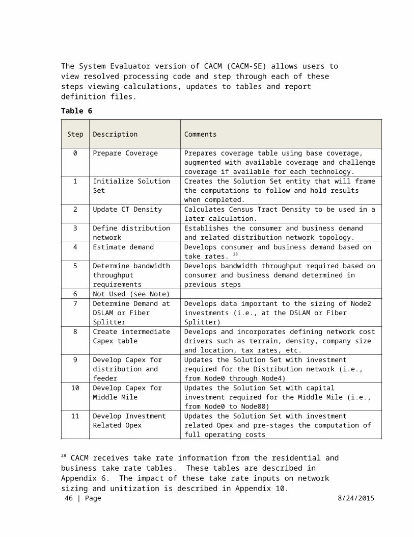
7 Appendix 1 – CACM Network Topology Methods
7.1. Introduction to CQLL
CACM makes use of two long standing models to develop the CACM network topologies: CostQuest LandLine (CQLL) and CostQuest Middle Mile (CQMM).
This appendix provides an overview of how the wireline topology was developed for CACM. As such, this section includes an overview of the underlying network loop topology platform (i.e., CQLL) as well as a discussion of modeling methods, a summary of key data sources and an overview of results.
Appendix 9 provides a corresponding overview of how wireline middle mile facilities are modeled using the CQMM platform. CQMM output is used by CACM to build the final comprehensive network topology which is in turn utilized in the development of a Solution Set.
CQLL produces a network topology (including cable lengths, equipment sizes and locations, etc.) for use in the CACM application. The modeled network includes all work efforts and components to prepare and place the asset / system for productive use within a network designed to provide the desired level of voice and broadband service.
Inputs, as outlined in this Appendix, are based on publicly available data and service area boundaries. Assumptions and engineering rules reflect real-world / current engineering practices, including how these practices are applied within specific terrain.
Finally, the central economic model is a widely accepted, modern approach to network modeling practices used throughout the industry.
CQLL is a next-generation network modeling platform. It models a forward-looking, optimized network based on a current demand analysis of network utilization. The CQLL platform uses a granular approach, adheres to spatial relationships and is based upon realistic implementations of common engineering guidelines.
At its core, the CQLL modeling platform is a “spatial” model. It determines where demand is located and “lays” cable along the actual roads of the service area to reach that demand point. In fact, a cable path can literally be traced from each demand location to the serving Central Office; a path that follows the actual roads in the service area.
CQLL determines the topology for wireline network components, across all categories of plant required to connect a specific service demand group (e.g. all locations or only connected locations) to their serving Central Office – and to provide voice and broadband-capable networks. The model assumes the 46 | Page 8/24/2015
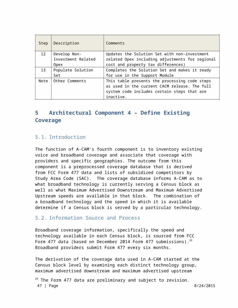
installation of forward-looking, commercially available telecommunications technologies and uses generally accepted engineering practices and procedures.
7.2. Accurate Bottoms-Up Design
Topologies created by CQLL are grounded in network connections among service demand Just like an engineer, the model tallies the necessary length and type of network facilities, including relevant network components and electronics, based on demand, Central Office locations and service architectures.
7.3. Developing Costs for Voice and Broadband Services
For the CACM application, CQLL was used to develop a GPON Fiber to the Premise (FTTp) network. More specifically, CACM’s FTTp topology is a design where the entire network from the Central Office to the demand location is entirely fiber optic facilities. In this design, the demand point is within 5,000 feet of the fiber splitter.
As noted below, prior versions of CACM provided for a Fiber to the DSLAM topology which included a blended copper and fiber design loop consisting of up to 12,000 feet of copper to the DSLAM and fiber from the DSLAM back to the Central Office.
7.4. Network Assets
The logic behind economic network modelling is derived from a realistic, engineering-based understanding of what drives; i.e., causes, investments in the environment (both physical and service demand) in which the network will serve.
As a broad guide, the following discussion provides the increments and drivers of the basic assets in the network modelled within the CQLL framework.
Loop: Wireline loop plant connects demand locations to Central Offices. The basic drivers of loop plant investment, including electronics, include all manner of demand and location. The loop is typically broken into a distribution portion and feeder portion. Distribution runs to demand locations from the Feeder Distribution Interface (FDI) described below while feeder runs to the Central Office from the FDI.
The distribution components, drivers, and nomenclature of the typical loop as modeled in CQLL are described below:
47 | Page 8/24/2015

Network Interface Device (NID) – The NID serves as a demarcation point between connected locations and the carrier’s distribution plant. In a Fiber to the Premise (FTTp) installation, an Optical Network Terminal and battery are used in place of a conventional NID.
Optical Networking Terminal (ONT) – An ONT is used to provide services to connected locations in an FTTP topology. An ONT is hosted by an Optical Line Terminal. The ONT is placed at each connected location.
Customer Premise Equipment (CPE) – CPE can be capitalized equipment that is placed on a customer premise. Its use is driven by a particular service (e.g., a modem for DSL). CPE investment is driven by the count of services, connected locations served, and ultimate ownership of the equipment.
Drop Wire (Drop) – For telecom deployment, the Drop is a cable sheath consisting of two or more pairs of copper wires which permanently connects the NID to a Distribution Terminal (DT). Essentially, the drop wire provides the connection between the premises and the distribution cable at the street. A drop wire can be buried or aerial and is driven by connected location demand. For Fiber to the Premise (FTTp) deployments, this drop is fiber, rather than copper, and connects up to the Fiber Service Terminal.
Distribution Terminal / Building Terminal (DTBT) – For telecom deployment, the Distribution Terminal (DT) is the point where the drop wires from several connected locations are connected to pairs in a larger cable. This cross-connect (sometimes called a “tap point”) can be located at a pole, handhole, buried splice, or pedestal. In some circumstances, the cross-connect or tap point can be a Building Terminal (BT). The BT acts as the demarcation point at a location where it is more effective to simply terminate a distribution cable at the demand location rather than using drop cables and NIDs. For FTTp, the DTs and BTs are replaced by Fiber Service Terminals and are fed by fiber cable.
For reporting purposes, the cross-connect point, whether it is a DT or BT or Fiber Service Terminal is described and tracked as a DTBT within CQLL. It is generically referred to as Node3 in topology structure diagrams.
Distribution Cable (DT-FDI) – The DT-FDI is the loop component that connects the DTBT with the feeder cable at the Feeder Distribution Interface (FDI). For FTTp designs, the distribution cable is fiber.
As the topology is exported to CACM, the CACM user inputs specify the percentage of distribution cable that is buried, underground or aerial through the entries in the plant mix table. The plant mix table is a portion of an Input Collection.
The major components of the feeder portion of the loop are described below:
Feeder Distribution Interface (FDI) – In copper loop architectures, the FDI is where distribution cables are connected to a feeder cable. The FDI allows 48 | Page 8/24/2015

any feeder pair to be connected to any distribution pair. (For reporting purposes, a portion of the FDI is assigned to distribution.) For FTTp designs, the FDI is replaced by the Fiber Distribution Hub (FDH) or Primary Flexibility Point (PFP).
Fiber Distribution Hub / FiberSplitter (FDH/PFP) – In an FTTp design, the fiber cable from the OLT in the Central Office or in the field is split at the FDH/PFP into 16 to 32 distribution fibers. These 16 to 32 distribution fibers then connect to ONTs at the premises.
DSL Access Multiplexer (DSLAM) –In an FTTd network, a DSLAM provides voice and broadband service capability and receives data from multiple DSL connections and most often aggregates the data onto a high speed Gigabit Ethernet (GigE) backbone.
The FDI, FDH/PFP and DSLAM are generically referred to as Node2 in topology structure diagrams.
Optical Line Terminal (OLT) – In an FTTp design, the fiber cable from the PFP terminates on an OLT. This OLT can either be housed in the Central Office or in the field.
Gigabit Ethernet (GbE or GigE) – A term implying the use of Ethernet to carry data at Gigabit speeds over Fiber Optic cable. For example, GigE is generally used to transport data from DSLAMs to the Central Office.
Feeder Cable (FDI-DLC and DLC-CO) – The feeder cable transports traffic, either voice or data, between the FDI/PFP and the Central Office in the telecom environment.
Ethernet Switch (eSwitch) – Internet Protocol traffic from each Service Area is routed to an Ethernet switch located in each Central Office.
The OLT and Ethernet Switch are generically referred to as Node0 in topology structure diagrams.
7.4.1 End User Demand Point Data
Within CQLL, the modeling exercise can begin with address-geocoded location data. Address geocoding is a method used to match an address to a location on a physical (real world) road network. Address geocoding is a well-established technique to derive a locational attribute, such as longitude and latitude or linear reference,39 from an address.
39 A linear reference is a method by which location is described in terms of a distance along a feature. A highway mile-marker is a type of linear reference. This is in contrast to a latitude, longitude which is a locational reference in terms of a grid placed upon the Earth’s surface.49 | Page 8/24/2015

CQLL then augments actual geocoded point data with surrogate locations for demand that cannot be located accurately. These surrogate locations are based upon generally accepted data sources (e.g., Census data), client-specific engineering and optimization rules, and standard industry practices.
In the current CACM implementation, CQLL uses geocoded information from GeoResults and Census information to derive estimated demand locations. As noted above, the surrogation of points is based upon generally accepted practices and occurs at the finest level of Census geography. That is, the surrogation of data takes place at the Census Block level using the roads and location counts within each Census Block. A technique called “stacking” provides for a relevant representation of demand located in apartment buildings. Care is taken so as not to place locations on specific types of roads such as interstate highways.
7.4.2 Service Areas
Using industry standard engineering rules, road distance and service demand information (e.g., DS0s, pairs, Living Units, etc.), service clusters are formed. A service cluster is a group of demand points which share a common loop network technology. For example, for a broadband network a service area could be described for all demand locations sharing the same DSLAM. Within each cluster, appropriate forward-looking digital equipment and copper and/or fiber cable is placed. Service clusters are used to surrogate: Distribution Areas (DAs), Fiber Serving Areas, Carrier Serving Areas, and Allocation Areas (FSA/CSA/AA).
7.5. Methods - Efficient Road Pathing and Networks
CQLL designs a network to serve demand locations within a service area (e.g., wire center, etc.) based on where they actually reside. The model “lays” cable along the actual roads in the service area to connect locations with their serving Central Office. As this section demonstrates, the network can be seen on a map of the actual roads in a service area. In fact, it will aid the reader in understanding the model if he/she begins to immediately consider visually the spatial layout of a road network. The figure below shows the road network for a typical service area.
50 | Page 8/24/2015
0
miles
2 4
Wire Center Boundary
Central OfficeRoads
LEGEND:
Figure 5 -- Road Network
7.6. Demand Data Preparation
The demand location data (both business and residential) was pulled from public sources. For residential data, GeoResults address data was trued up with Census household counts. For business data, GeoResults address data was used. In each case, counts of locations by address and/or Census Block are provided. Before the location data can be used, it must be located on the earth’s surface, along a road path so that the network routing algorithms know where to route. For demand location that is non-address or cannot be geocoded, a random placement algorithm is used to place the demand locations along the roads of the Census Block. Care is taken so as not to use roads that are restricted (e.g., interstate highways).40 In addition, multifamily and buildings containing residential and business demand are tracked. This allows CQLL to identify the appropriate multi-dwelling equipment rather than replicate single demand unit equipment.
Figure 6, presents a section of the view shown in Figure 7 with demand locations shown as circles. In this example, these circles represent all of the service demand points (e.g., both business and residences). The demand and service data are now ready for processing by CQLL.
40 TIGER road types used by the model include S1200, S1400, S1640 and S1740.51 | Page 8/24/2015

0 200
feet
400
Customer LocationRoads
LEGEND:
Figure 6 -- Demand Locations
7.7. Efficient Routing
Using the demand locations and the road network, specifically designed and reviewed algorithms determine network routing and placement based upon standard industry engineering rules. As a first step, CQLL uses an Efficient Road Pathing (“ERP”) algorithm to develop the optimized routing from the Central Office to all demand locations. Once a full service area ERP is determined, CQLL develops natural clusters by linking demand points that are close together (e.g., neighbors). These neighbor groups are further combined with other nearby demand clusters to form larger clusters (“neighborhoods”). This process continues until the clusters reach the limits of length and/or capacity as specified by the engineering design (e.g., 5kft max length from the fiber splitter). Once all demand locations to be served by a host node are determined, appropriate components such as Feeder Distribution Hubs (FDHs), Fiber Nodes and Feeder Distribution Interfaces (FDIs) are located within each serving area. Once the serving nodes are placed within these “remote” served serving areas, an optimal path is formed to the hosting Node. The path within each serving area then becomes the distribution cable path. This process continues until all portions of the service area have been “clustered”.
For those demand locations served by a terminal in the Central Office, a distinct ERP is determined. Once the main Central Office served areas are determined, an ERP is created. These tree paths are then ‘walked’ to determine points at which Feeder Distribution Interfaces (for copper areas) or Fiber Distribution Hubs (for fiber served areas) terminals are to be placed. 52 | Page 8/24/2015

These placements are driven by user inputs guiding demand location counts and distance limits.
As a final step in the pathing algorithms, an ERP for feeder plant is determined. That ERP links the nodes outside of the Central Office (e.g. DSLAM or FSH, Node2) to the Central Office (CO). In CACM 4,0, changes were made to the feeder pathing algorithms. This improves feeder path determination in areas with multiple roads.Figure 7 depicts a distribution network created by the process based on the optimized ERP approach. Figure 8 depicts the same type of information for the feeder network.
LEGEND
FDI LocationDLC LocationDT/BT LocationRoadsFeeder RouteDistribution RouteWire Center Boundary
Figure 7—Distribution Plant
53 | Page 8/24/2015

0
miles
Central OfficeDLC LocationRoadsFeeder RouteWire Center Boundary
LEGEND
1.5 3
Figure 8 -- Path for Feeder Plant
After the serving areas and optimal routings are determined, engineering rules guide the installation and placement of electronics, such as Fiber Nodes, DSLAMs, and Central Office Terminals.
Once the spatial layout of the network is determined, CQLL’s Configuration Process connects the network components. This entails the determination of cable sizes, identification of service points requiring special engineering, and selection and sizing of Node2 type. Once the network is configured, CQLL summarizes the network topology information to create the source file for the CACM application. In this summarization, the information about the network build is related to / associated with the relevant Census Block records. As such, each Census Block record captures the size of the main serving terminal (e.g., DSLAM, FDH, etc.), the demand at the Central Office, the length of the feeder and distribution cable and the portion attributable to the Census Block, and other pertinent information relevant to the network build. In CACM 4.0, modifications were made to the routines that develop accumulation calculations of Feeder Fibers for GPON Splitters and Special Access services. Modifications were also made to calculation formulas consistent with changes described in prior versions of CACM release notes.
CACM allows an end user to review these two summary files by wire center. These reports are available as Audit reports, Audit Network Design Dist or Audit Network Design Feeder.
54 | Page 8/24/2015

7.8. CQLL Network Engineering, Topologies and Node Terminology
CQLL develops investment estimates for wireline loop plant. The loop is the portion of the telecommunications network that extends from the Central Office (CO) to the demand location.
A loop extends from a demand location (a business or housing unit). It can be terminated on specific customer premise equipment, CLEC equipment or any multitude of routers, gateways or specialized equipment necessary to support IP driven services like VoIP.
CQLL designs a network using forward-looking technologies and design principles. To meet the heterogeneous engineering characteristics of today’s service providers, CQLL is capable of modeling different wireline topologies. This section describes potential network topologies and lists the Node reference for each. It is helpful to understand the unique Node naming conventions as these descriptions carry forward to audit reports and cost / investment information.
In the CACM network designs, the references to network topology have been standardized by using the values of Node0 through Node4. Node identifiers are used to help bridge the understanding of functionality across the differing technologies (wireless and various forms of fiber and hybrid fiber solutions) that are used in CACM. The “nodes” are significant in that they represent the way in which costs are assigned / aggregated to enable comparisons across technologies. Node diagrams for both FTTp and FTTd designs are provided for reference.
The FTTd design, available in earlier versions of CACM is shown in Figure 9.
55 | Page 8/24/2015

Figure 9--FTTn and FTTd Topologies
56 | Page 8/24/2015

The second IP based topology is Passive Optical Network (GPON) FTTp (Fiber to the Premise), as depicted below.
Figure 10--FTTP topologyIn this topology an ONT (Optical Network Terminal) is placed at the demand location, along with a battery for backup power. Fiber cable then connects to the Central Office. Along the path, the fiber is concentrated at the PFP (Primary Flexibility Point) or FDH (Fiber Distribution Hub) in a typical 32 to 1 ratio. At the Central Office, the fiber from the PFP or FDH terminates on an OLT (Optical Line Terminal). The traffic is then sent to an Ethernet switch. IP packets are routed to the IP network via a connection to a router. This gateway router can be in the Central Office or can be located at an intermediate office to support multiple Central Offices.
57 | Page 8/24/2015

7.9. Key Network Topology Data Sources
Network Topology development requires data inputs and modeling assumptions unique to CACM’s requirements and assumptions. Input data and relevant sources are outlined below.
7.9.1 Service Area Engineering Input data
Public domain and commercially licensed data products provide the foundation for the CQLL model. This included service area boundaries, Central Office locations and demand sources.
Service Area boundaries o GeoResults, 4th Qtr 2012.
Central Office locationso GeoResults, 4th Qtr 2012.
7.9.2 Demand data
The goal of CACM was to produce investment for all potential voice and broadband demand locations; CQLL develops a network serving all potential residential and business locations.
Residential demand was based upon GeoResults (3rd Qtr. 2012) data that provided residential and business address data. Residential counts in each Census block were trued up to Housing Unit counts from 2011 Census data. Business demand data was also derived from GeoResults (3rd Qtr 2012).
7.9.3 Supporting Demographic Data
CQLL requires several additional data sources to support road pathing and demographic analysis.
These data sources are described below:
Roadso Source: US Census TIGERo Vintage: 2010
Census Blockso Source: US Census TIGERo Vintage: 2010
Demographic Estimateso US Census Housing Unit and Population Estimateso Vintage 2011
58 | Page 8/24/2015

8 Appendix 2 – CACM Middle Mile Network Topology Methods
8.1. Introduction to CQMMIn concert with the development of loop topologies using CQLL, the middle mile methodology and approach of CACM uses components of the CostQuest network modeling platform (CQMM).
The middle mile is that portion of the network that provides a high capacity transport connection from Central Office to Central Office (Node0 to Node0) and/or Central Office to Regional Tandem (Node0 to Node00).
In CACM the middle mile is assumed to extend between the service provider’s point of interconnection with the internet and the service provider’s point of interconnection (“POI” or CO) with the second and last mile network built to support end user broadband demand locations in unserved areas. This relationship is illustrated in the Figure 11.41
41 In Middle Mile diagrams, the DSLAM is preserved to indicate how Middle Mile architecture was used in prior versions of CACM. Given the FTTp CACM topology, a DSLAM node would not be present.
59 | Page 8/24/2015
Figure 11--Middle Mile Architecture
The material that follows provides additional information on how middle mile investments are developed within CACM.
The approach used to determine middle mile equipment required – and then to compute the related investment costs – is centered in the spatial relationship between the service provider’s point of interconnection (POI or CO) with the second and last mile network (designated as a Central Office) and the service provider’s access to a Tier 3 internet gateway (a surrogate for such access is assumed to be at a regional access tandem (“RT”) or RT ring).
Central Office Location: the location of each Central Office (also referred to as POIs, and/or Node0s) is obtained from the GeoResults database. The results of this approach align with the Central Office/Node0 locations used in the underlying CQLL Network Topology model used to create the local loop network, including last and second mile related equipment and investments.
60 | Page 8/24/2015

Regional Tandem Location: Regional tandem (RT) locations (and the relevant feature groups deployed) were obtained from the LERG® database. Each tandem identified as providing Feature Group D access in LERG 7 is designated an RT. As with COs, a latitude and longitude is identified for each RT.
The underlying logic (and the process) of developing middle mile investment requirements is grounded in the assumption that the Tier 3 internet peering point is located at an RT or on the RT ring – meaning that if the modeled design ensures each Node0 is connected to an RT, the corresponding Node0 demand has access to the internet.
Given this baseline data on CO and RT locations and working under the assumption outlined above, the middle mile processing logic proceeds as follows:
The Middle Mile process is run state by state. All Node0’s in a state are homed to an RT in that same state
Within a state, each Node0 is assigned to its nearest RT (Node00) to create the initial spatial relation of (“parentage”) Node0s to RTs. Node0s must be in the same state as their related Node 00.
Node0 records are then routed to other Node0 records with the same Node00 parent using a spanning tree approach based on the shortest (most efficient) distance routing back to their proper Node00 record.
The Node00 records within the same LATA are routed together in a ring. To ensure an efficient (and hence ‘most likely’) design the shortest ring distance is used. The shortest ring is chosen by starting at each Node00 point and storing the ring distances. After stepping through each potential ring route, the shortest ring distance is then used for further computations.
With that information in hand, CACM develops middle mile costs thru the following steps:
a. The distance of the RT rings is attributed to each Node0 on the ring in proportion to the number of locations at each Node0 as compared to the total locations for all the Node0s attached to the RT Ring. For each spanning tree connection, distance is calculated as follows. Where a road distance is available, 42 the road distance is used unless the ratio of the road distance to airline distance is > 3.04. In that case the airline distance x 3.04 is used. If the route is classified as partially submarine (see section8.4), 1.2 x the airline distance is used to develop the
42 Road distance is calculated using ESRI Network Analyst, version 10.1
61 | Page 8/24/2015
overall distance between the points. Within CACM, the final middle mile distances are multiplied by the TreeToRingRedundancyFactor in the Capex input (the factor is currently set to 1.2).
b. The distance on the Node0 tree back to the RT is attributed much in the same way as the loop feeder routing. That is, CACM attributes each route based on the cumulative locations that can use the route.
c. For electronics, CACM captures the broadband routers (it is assumed that each CO/POI will connect to two routers to provide redundancy) which connect up to the fiber at RT/Tier 3 location. Additional electronics of the RT/Tier 3 or the RT ring are not included as part of the costs.
d. For the fiber placement, CACM assumes a portion of the conduit, buried trenching and poles already exist for the local access network (this sharing is controlled in the Capex input workbook). As such, only a portion of additional costs for conduit, buried trenching and poles is captured for middle mile. CACM does retain the full cost for fiber which supports the end user broadband-capable network.
e. From the total middle mile costs that are calculated, CACM captures a portion of the costs (some costs are assumed to be absorbed by uses other than CACM voice and broadband services, e.g., special access services). This sharing assumption is controlled in the Capex input workbook.
f. Finally, CACM relates the middle mile cost to each Census Block (the basic unit of geography in CACM) based on the proportion of potential demand locations in the Census Block (as compared to the total locations in the POI/CO/Node0 serving area).
8.2. Middle Mile Undersea Topologies for Price Cap Carriers in Non-Contiguous Areas
For price-cap carriers who need undersea links to the contiguous United States, CACM calculates costs associated with the undersea link back to the contiguous United States.
The Undersea tab of the CAPEX workbook provides the following inputs: Undersea cable investments including repeater electronics Landing station investments including electronics Route distances Route broadband traffic percentage use factors
62 | Page 8/24/2015

Investments calculated within the undersea portion of the CAPEX workbook represent additive investments to the middle mile (Node0 to Node00) portion of the network for non-contiguous areas. These investments capture the costs of undersea cable and landing station investments needed to transport traffic from landing stations in non-contiguous areas to landing stations in the contiguous U.S.
The total route investment is calculated as (Route Distance x Cost Per Foot) +2 x (Landing Station Investment) for each route. It is assumed that each non-contiguous area is connected by two routes to provide redundancy.
Undersea fiber optic cable inputs were developed on a per foot basis for material and labor based on publicly available data for an undersea cable system connecting Alaska with the U.S. mainland.43
In addition to the fiber optic cable investments, Landing Station investments are based on publicly available data.44 CACM assumes 2 landing stations per route. The total estimated investment (equipment, land and buildings) is for stations at both ends of each undersea route. This investment is broken down between equipment, land and buildings.
After the total route investment is developed, the total route investment is multiplied by the averages listed in the table shown below, which represent the percentage use, utilized for voice and broadband.45
8.3. Development of Undersea Percentage Use FactorsPercentage use factors reflect the portion of the total route utilized by the CACM network.
To develop these factors, total CACM busy hour bandwidth demand was compared to the actual deployed capacities of current undersea routes, both total route capacity and highest lit capacity.46 Table 8, below, shows both comparisons; the average of both is the value used as the percentage use in CACM.
43 Presentation available at http://akorn.alaskacommunications.com/#, estimates total construction cost. The submarine values for Alaska were not adjusted with Regional Cost Adjustment factors. 44 See slide 29 of http://hmorell.com/sub_cable/documents/Basics%20of%20Submarine%20System%20Installation%20and%20Operation.pdf45 The percentage use factor inputs are located in the Capex workbook, undersea worksheet.46 CACM calculates the demand for the modeled network assuming that all end users are simultaneously consuming the total busy-hour offered load. Accordingly, estimated demand is based on CACM locations * Take Rate * Bandwidth (CACM BHOL input).
63 | Page 8/24/2015
Table 8--Percentage UseAREA DEMAND
(Gbps)HIGHEST TOTAL CAPACITY (Tbps)
% DEMAND to TOTAL CAPACITY
HIGHEST LIT CAPACITY (Gbps)
% DEMAND to LIT CAPACITY
AVERAGE
Hawaii 213.6 6 3.956% 2,000 11.867% 7.91%North Marianas Islands (Guam to Oregon)
7.7 7.68 0.111% 5,120 0.166% 0.14%
Puerto Rico
587.9 80 0.816% 310 100% 47 50.00%
U.S. Virgin Islands (Puerto Rico to Florida)
20.0 80 0.028% 310 7.168% 3.60%
For routes that are utilized for international traffic, CACM estimates the investment that carriers will face in securing transport to and from the contiguous United States by applying the percentage use value to the CACM-calculated total route investment. Because the Alaska route and the Northern Marianas to Guam portion of the Northern Marianas route are not shared with any international traffic, CACM includes 50 percent of the costs of connecting Alaska to Oregon and Washington, the Northern Marianas to Guam, and the U.S. Virgin Islands to Puerto Rico, which is the default middle mile allocation in CACM.48
Investments are converted into costs based upon the Underground Fiber Optic Annual Charge Factor.
8.4. Submarine Topologies for Price Cap Carriers in Non-Contiguous Areas
In addition to the airline distances and road distances in non-contiguous areas, two additional data fields are available to middle mile processing code. 47 CACM caps lit capacity at 100 percent. Because there is unlit capacity available or coming on line, it is assumed that it would not be economically reasonable to build two or more new cables.48 CACM assumes that the other 50% of costs are allocated to special access and private line services, and supported by revenues from those services.
64 | Page 8/24/2015

Submarine distance; and, An indicator of whether the route is visually on the same or different
land masses. Within CQMM a route is classified as partially submarine where there is no connection between the land masses. In a separate analysis, there was one additional route that was classified as partially submarine, given that the road distance was over 20 times longer than the airline distance.
For each route classified as partially submarine, two beach manholes are placed. Submarine cabling investment is used for the submarine segment while land based cabling is used for the remainder. Submarine cable investment is not shared with other utilities nor impacted by regional cost adjustment.
Submarine investment is converted into costs based upon the Underground Fiber Optic Annual Charge Factor.
65 | Page 8/24/2015
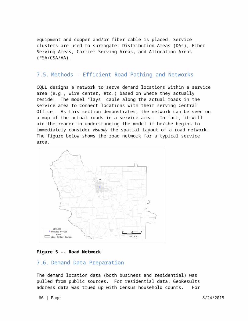
9 Appendix 3 – Data Source and Model Application Summary
The table below provides a summary (inputs grouped by category) of the major data inputs to the CACM along with the underlying source for that data and a reference to its use within the model.
Table 9
Data Category
Model Variables Data Source Wireline Coverage
Capex
Opex
Census boundaries
Full Census Block; full Census Block Group; full Census Tract; full Census County; Census State
TIGER\Line 2010
X X x
Service Area boundaries and Central Office locations
Service Area boundaries, codesand Central Office points, as adjusted by public comment and USAC review
GeoResults 4Q 2012
X X
Geographic characteristics
Land area; total road length;
TIGER\Line 2010
X X
Terrain Terrain characteristics USDA, NRCS-STATSGO, SSURGO
X X
Housing Units
Occupied housing units; total housing units; total households by block. Adjusted by Census Population and Housing Unit Estimates
Census 2010, SF1 housing units. Census Population and Housing Unit Estimates, 2011
X X X
Provider size and organizational structure
Corporate ownership; size of parent company; number of wire centers operated by carrier
ABC Coalition Members, Support Feedback, FCC, USAC
X X X
66 | Page 8/24/2015

Data Category
Model Variables Data Source Wireline Coverage
Capex
Opex
Company Opex financial data
A wide array of company-specific financial information (and underlying business volumes) from public and subscription service sources. Data centers on operating expense by category (e.g., maintenance, sales, interconnection, sales and marketing, G&A, bad debt, taxes, etc.).
Data sources available in methodology
X
High capacity locations
High capacity locations represent high demand business points and will be used to improve business location points for sizing the network. Community Anchor Institutions (CAI) taken from National Broadband Map.
GeoResults 3Q2012 National Building Database and Detail Business File. CAI from National Broadband Map (June 2012)
X X
Wireless tower location
Wireless tower locations represent locations requiring fiber service and are used to supplement business and residential locations for sizing the network.
CostQuest proprietary tower database
X X
Fixed Wireless broadband service
Fixed wireless provider broadband speed coverage within a Census Block (Transtech 70), as adjusted based upon FCC Form 477 reporting data.
FCC Form 477 (December 2014),
X
67 | Page 8/24/2015

Data Category
Model Variables Data Source Wireline Coverage
Capex
Opex
Telco broadband service
Telecommunications provider broadband speed for wireline area coverage within a Census Block (Transtech 10,20,30,50)
FCC Form 477 (December 2014),
X
Cable broadband service
Cable provider broadband speed for cable area coverage within a Census Block (Transtech 40,41,42) as adjusted based upon FCC Form 477 reporting data.
FCC Form 477 (December 2014),
X
68 | Page 8/24/2015

10 Appendix 4 – CACM Data Relationships
The schematic provides an overview of how data are organized and related within CACM. The diagram is designed to illustrate at a high level the relationships between inputs and the resulting Solution Set.
69 | Page 8/24/2015

Figure 12--CACM System Schematic
70 | Page 8/24/2015

11 Appendix 5 – CACM Processing Schematic
Figure 13--CACM Processing
71 | Page 8/24/2015
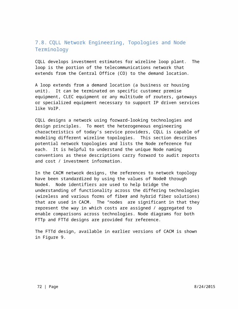
72 | Page 8/24/2015
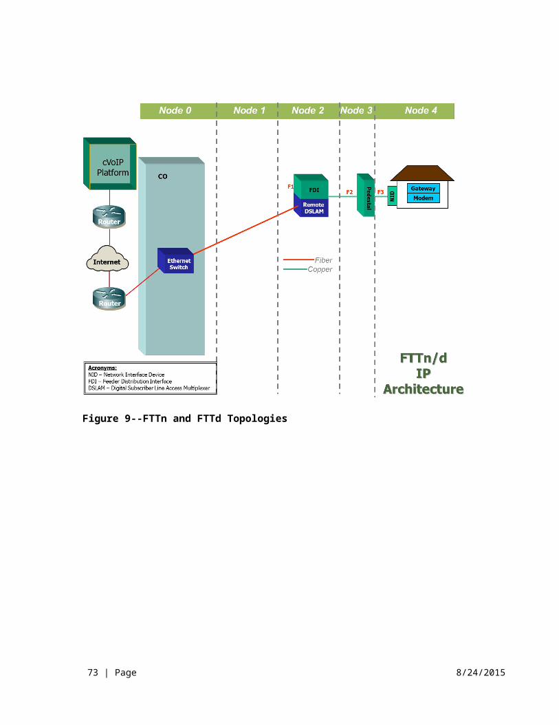
The diagram in Figure 13 is color coded to illustrate how information can flow through CACM. Specifically, the grey colored objects reflect a system input (e.g., an input table) that is driven by a user. Once that input table is loaded into the system, it becomes part of an input collection then a user generated Solution Set. In contrast, many users run CACM without modifying any inputs and are reliant on default (blue) system objects.
From left to right Figure 13 shows that a group of input tables (i.e., Input Collection) is used by the Cost to Serve Module. Users can either use the default input collection or load their own tables to suit particular analytic needs. The files which constitute an Input Collection are shown in Figure 13 and further described in Appendix 6. The Input Collection is where users provide information about the cost of plant such as structure (e.g., Poles, Conduit) or costs of equipment (e.g., DSLAMs, Fiber Splitters).
Along with an Input Collection, the Cost to Serve module also requires information on the geographic scope of analysis, the type of network to build and two other toggles to create a Solution Set49. Once the Solution Set has run, several types of reports are available from CACM. Additional information about CACM reports is also available in the User Guide.
Also note on Figure 13 several orange symbols. These orange components represent additional databases which are preprocessed and available as inputs into CACM.
49CACM allows you to export a Solution Set as part of the Audit Solution Set report. The audit report contains the portion of a Solution Set specific to the user entered Service Area name.
73 | Page 8/24/2015
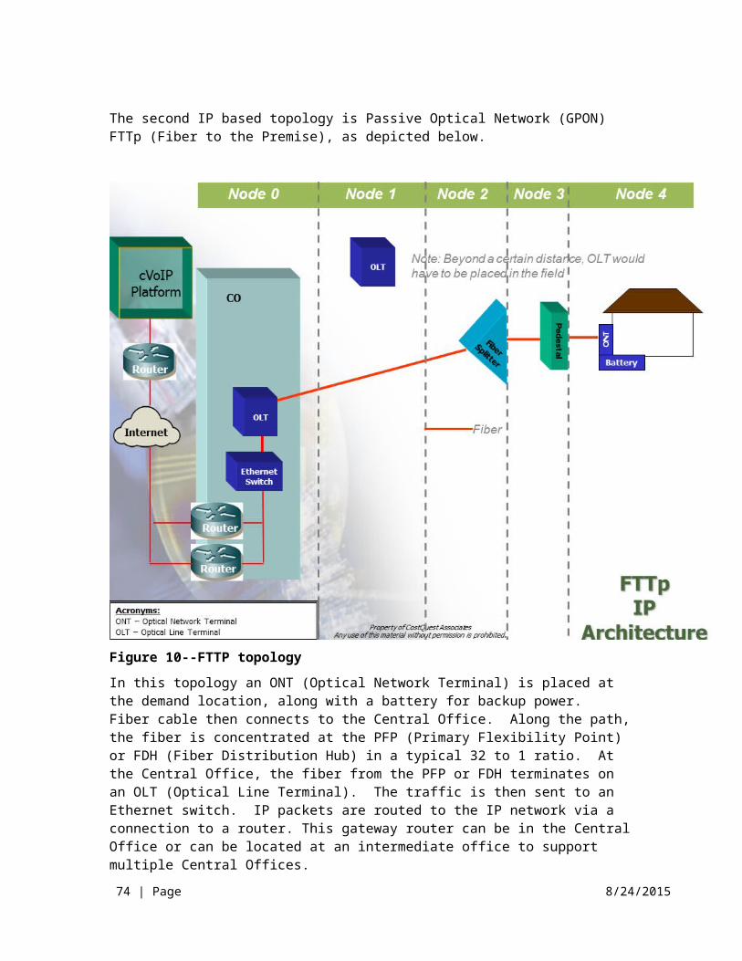
12 Appendix 6 – CACM Input Tables
The inputs which form the basis of an input collection are available as a download from the CACM website.
Annual Charge Factor (ACF)o This table captures the Annual Charge Factors that convert Investment
into monthly costs. The values loaded into CACM are produced by CostQuest’s CapCost model which is available for download. The basis of the model is the economic determination of the depreciation, cost of money, and income taxes associated with various plant categories. The calculation incorporates industry standard procedures, such as Equal Life Group methods, inclusion of future net salvage, impact of deferred taxes, and mid-year conventions.
Key inputs into the derivation are lives of plant, assumed tax lives, survival curve shapes, cost of money, cost of debt, debt/equity split, and future net salvage
o Uses depreciation lives consistent with those prescribed by the FCC’s Wireline Competition Bureau’s latest general depreciation in CC Docket No. 92-296
o How Used: Converts Investment into monthly values of Depreciation (DEPR), Cost of Money (COM), and Income Taxes (TAX)
Bandwidtho Provides the busy hour bandwidth o Used to size appropriate network componentso How Used: Based upon current inputs, Bandwidth is currently not a
driver of any capex investment or opex cost.
Business Take o How Used: Derives the voice and data demand for the business
market50
Capexo Provides the material and installation costs for the plant buildo Data are applied against the network topology data to derive total
build-out investment levelso Inputs capture technology, network node, network function, and plant
sharing.51 Within the CAPEX workbook, all Material inputs are material
50 The business and residential take rate inputs can impact CACM in two ways. First, they can impact how components of the modeled network are sized. Second, they can impact how the total investment and resulting costs are unitized. See Appendix 10.
51 See Appendix 7, Methodology for additional information on Plant Sharing.
74 | Page 8/24/2015

only. As an example, the OLT inputs found on the FTTp Material worksheet are material prices only. EF&I is included in the “Total Material Loadings” and “Engineering Rate” on the Labor Rates and Loadings” worksheet. The model always adds in labor costs – either through direct inputs such as the Material Labor worksheet for telco placing and splicing costs and the Structure Labor worksheet for OSP contractor structure placing costs, or through the use of the EF&I factors on the Labor Rates and Loadings worksheet.
o How Used: Values which derive the total capex.
COSize Adjustmento Provides the user the capability to adjust the assumed purchasing
power of small, medium, and large providerso The current inputs assume that all providers can achieve the same
purchasing power (either as a result of their size or their ability to buy as a consortium)
o Adjusts up or down the Capex costs in the model, current inputs are set to 1
o How Used: In the current release of the model, COSize Adjustment table is used but the value is set to 1.
OCNCoSizeo Provides correspondence for OCN, company size category and SAC.o How Used: Categorizes the size of each company.
Opexo Provides the estimated operation costs to run and maintain voice and
broadband-capable networks.o How Used: Values help to develop the operational cost development.
PlantMixo Provides the estimated mix of facilities by type: aerial, buried, and
undergroundo How Used: Determines the mix of facilities required to serve an area.
PlantMix Buried Conduito Provides values to be used which represent the percentage of buried
placements to become buried placement in conduit. o How Used: The values in this table indicate the percentage of buried
placements to become buried placement in conduit. As an example, if the table value is 1 (100%) for Distribution (Dist) then 100% of the corresponding distribution buried plant placements will be buried in conduit. To preserve backward compatibility with earlier input collections, a non-calculation impacting version of this table is available, PlantMixBuriedConduit NonState. This ‘NonState’ version has been associated with input collections created before CACM 4.0. If desired, a user can select PlantMixBuriedConduit NonState when
75 | Page 8/24/2015

creating a CACM 4.0 solution set. A copy of PlantMixBuriedConduit NonState is available for review within the Input Collection published on the CACM website.
Ptaxo Sourced from property tax rates in each state compared to a national
averageo Provides the impact of property tax on the G&A operation costs given
the difference of the state rates versus the national averageo Captured in the multiplier used for the operational elemento How Used: Provides an index value to capture the impact of property
tax in the operation costs.
RegionalCostAdjustmento Sourced from third party source – RSMeans (2011)o Provides the estimated difference in the cost to build and operate in
each part of the countyo Used to drive differences in Capex and Opex costs due to labor and
material cost differences across the country Applied to All Capex and indirectly to specific Opex components
that are derived from Capexo How Used: Captures material and labor costs difference at ZIP3 level.
StateSpecific Capexo Provides an input source for situations in which a state specific
CAPEX input is required.o How Used: When State Specific Capex toggle is set to “Yes”, CACM
reads the values in this table and uses them when processing the States provided in the StateSpecific input workbook. To preserve backward compatibility with earlier input collections, a non-calculation impacting version of this table is available, StateSpecificCapex NonState. This ‘NonState’ version has been associated with input collections created before CACM 4.0. If desired, a user can select StateSpecificCapex NonState when creating a CACM 4.0 solution set. A copy of StateSpecificCapex NonState is available for review within the Input Collection published on the CACM website.
StateSalesTaxo Sourced from appropriate sales tax rates for telecommunications plant
in each stateo How Used: Impacts Capex derivation, applies State Sales Tax.
Residential TakeRate52
52 The business and residential take rate inputs can impact CACM in two ways. First, they can impact how components of the modeled network are sized. Second, they can impact how the total investment and resulting costs are unitized. See Appendix 10.
76 | Page 8/24/2015

o How Used: Derives the data and voice demand for the residential market
77 | Page 8/24/2015

13 Appendix 7 – CACM Plant Sharing Input Walkthrough
This material provides an overview of the source and use of the input tables in the Plant Sharing tab of the Connect America Fund Cost Model (CACM) Capex input workbook. The order in which we describe the components below is designed to explain the interaction between these functions and is not necessarily the sequence or flow in terms of how the tables are used within CACM.
Modern telecom networks increasingly enjoy the benefits of sharing facilities and capacities across different services to different demand groups in different geographies/locations. The ability to leverage network investments in this way is vital to the network’s economic performance through time. Within the context of CACM, it is important that mechanisms exist to share facility and structure costs across the relevant network functions and geographies (e.g., ultimately, across Census Blocks).
As outlined below, there are four components of the CACM plant sharing function (i.e., four types of facilities sharing):
Sharing Between Distribution and Feeder Sharing Between Providers Sharing Of The Middle Mile Network Sharing Of Middle Mile Routes Associated with Voice and Broadband
Each of these components is explored further in the material that follows. In each section we describe the type of structure sharing and the CACM Logic which then employs and processes those inputs.
13.1. Sharing Between Distribution and Feeder
This input table provides the percent of common route (both feeder and distribution on the same route) that shares structure in three density categories (i.e., Rural, Suburban and Urban) across three types of plant (i.e., Aerial, Buried and Underground).
Density
% of common route that that shares structure
Aerial Buried Underground UOMRural 78% 41% 67% percentSuburban 78% 41% 67% percent
Urban 78% 41% 67% percent
CACM Logic: The schematic that follows represents a typical network topology developed by CACM. For additional information on how network topologies are developed within CACM please refer to the CACM Methodology.
78 | Page 8/24/2015

In this schematic distribution pathing is represented by golden lines, feeder pathing is represented by blue lines, and pedestals are represented by gray boxes.
The expanded diagram to the right shows a typical Node2 cluster (e.g., the pedestals served by a specific splitter in an FTTp network). Within the topology creation process, each segment (network node to network node) is tracked with information on:
Density of the area in which the segment resides Terrain of the area in which the segment resides Length of the segment Amount of segment that is shared between distribution and feeder routes
Using the schematic above as an illustration, the discussion that follows explains how CACM develops structure sharing "Between Distribution and Feeder".
Consider two segments (a) and (b) labeled in the expanded diagram at right in the schematic above. Each segment is 1000 feet long. Segment A is ONLY a distribution route and Segment B is BOTH a distribution route and feeder route (100% of the route is shared). To simplify our example, assume the plant mix for both segments is 50% aerial and 50% buried and further assume that the area is Suburban.
When developing the topology, fiber routes are planned for each segment. For Segment A, 1000 feet of fiber is installed for the distribution plant. For Segment B, 1000 feet of fiber is installed for the distribution plant AND 1000 feet of fiber is installed for the feeder plant.
With these requirements in mind, structure is now designed for each segment. For Segment A, based on the 50/50 split of Aerial and Buried, 500 feet of trench will be dug and poles for a 500ft route will be placed. For Segment B, both feeder and distribution cables are being placed. However, the inputs provide for the fact that
79 | Page 8/24/2015
there will often be timing differences in design and placement and there is a probability that different forms of structure will be used between feeder and distribution. As such, we will likely need more than 1000 ft of overall structure (though less than the 2000 feet of structure that would be required if the feeder and distribution plant are built entirely independently of one another).
To arrive at the structure needs for Segment B, we refer to the "Between Distribution and Feeder" table to guide the calculation.
Specifically, referring to the input values in the table above, for the 500 feet of required Aerial distribution structure and the 500 feet of required Aerial Feeder structure:
(100% - 78%) , or 22% is dedicated or non-shared…or 110 feet and 78% is shared…or 390 feet.
Since both feeder and distribution are sharing the same pole 78% of the time (or 390 feet for this 500’ span of cable), we assign 1/2 of the 390 feet (i.e., 195 feet) to Distribution and ½ of the 390 feet to Feeder. The total Aerial structure feet for distribution is then 110 feet of dedicated and 195 feet of shared for a total of 305 feet of distribution structure; and, for feeder the total Aerial structure feet is 110 feet of dedicated and 195 feet of shared for a total of 305 feet of feeder structure.
Again, referring to the input values above, for the 500 feet of required Buried distribution structure and the 500 feet of required Buried Feeder structure:
(100% - 41%), 59% is dedicated or non-shared…or 295 feet and 41% is shared…or 205 feet.
Since both feeder and distribution are sharing the same trench, we assign 1/2 of the 205 feet (i.e., 102.5 feet) each to Distribution and Feeder. The total Buried structure feet for distribution is then 295 feet of dedicated and 102.5 feet of shared for a total of 397.50 feet of distribution structure. For feeder, the total Buried structure is also 295 feet of dedicated and 102.5 feet of shared for a total of 397.50 feet of feeder structure
13.2. Sharing Between Providers
This input table provides the percent of cost attributed to a studied carrier across three density categories (i.e., Rural, Suburban and Urban) across three types of plant (i.e., Aerial, Buried and Underground). These inputs reflect the fact that portions of structure costs may be shared with other parties (attachment to third party poles rather than owning poles, sharing of joint trenching costs, etc.)
Density% of Cost Attributed to Studied Carrier
Aerial Buried Underground UOMRural 48% 96.25% 95.78% percentSuburban 48% 80.00% 79.53% percent
80 | Page 8/24/2015
Urban 48% 76.25% 75.78% percent
CACM Logic: Using the schematic and overall assumptions described above and from the logic used for the sharing "Between Distribution and Feeder" we know the structure distances. With this information in hand the cost of the structure attributable to the network of the provider under study is developed using the inputs of the "Structure Sharing" table and is rather straight forward as follows:
For the aerial routes, 48% of the aerial structure (poles) costs are assigned to the providerFor the buried and underground routes (using suburban values as an example), 80% of the buried trench and/or underground structure is assigned to the provider53
13.3. Sharing Of the Middle Mile Network
This input table provides the percent of a interoffice, or middle mile, route that requires dedicated structure (as opposed to sharing structure with feeder and/or distribution cables) across three density categories (i.e., Rural, Suburban and Urban) across three types of plant (i.e., Aerial, Buried and Underground).
Density% of route that is dedicated structure
Aerial Buried Underground UOMRural 37% 71% 26% percentSuburban 22% 64% 19% percent
Urban 14% 56% 11% percent
CACM Logic: Using the schematic and overall assumptions provided above the CACM logic for the attribution of costs regarding interoffice (IOF)/Middle Mile facilities is described below.
For interoffice routes, the routing runs from Central Office to Central Office. The logic for feeder and distribution structure captures the full cost of structure within the wire center. It is likely that the interoffice routes will often run along the same routes as used by the feeder and distribution and use the same structure. This table reflects the percentage of the time that interoffice cables do not share structure with feeder and/or distribution cables. In other words, this factor captures a similar kind of sharing as was captured in the section on sharing between distribution and feeder (though these figures represent the amount of dedicated middle mile structure; while the feeder-distribution sharing figures represent the amount of structure that is shared.
53 This means, for example, that there is only a 20% chance that an electric, cable or other companies will want to lay fiber along a given route at the same time when the provider has a buried trench open or underground conduit duct available. The sharing of poles is assumed to be much more prevalent (less cost assigned to providers) because other companies do not need to be deploying facilities at the same time in the same place to share the cost of aerial facilities.
81 | Page 8/24/2015
The inputs in this table reflect when dedicated structure will be incurred solely for the interoffice routes.
For aerial and underground structure, this sharing will likely be much higher than for buried structure, as shown in the low amount of dedicated structure assumed in the input.
For example, in an urban area the model assumes that structure needed for interoffice routes will be shared with distribution and/or feeder cables (100%-14%), or 86%, of the time and those structure costs are already included in the feeder and/or distribution cost calculations. For 14% of the urban interoffice route distances, the model assumes that separate structure is required for the interoffice cables.
13.4. Sharing of Middle Mile Routes Associated with Voice and Broadband
Input values (see table below) are based on the assumption that there are two major groups of services traversing the interoffice network: voice/broadband and Special Access services. CACM only includes the interoffice costs associated with the voice/broadband services. This input table provides the percent of an interoffice route that is attributed to voice/broadband across three density categories (i.e., Rural, Suburban and Urban) across three types of plant (i.e., Aerial, Buried and Underground).
Density% of route that is attributed to Broadband
Aerial Buried Underground UOMRural 50% 50% 50% percentSuburban 50% 50% 50% percent
Urban 50% 50% 50% percent
CACM Logic: The CACM logic for the attribution of costs regarding the assignment of Middle Mile Routes with Voice/Broadband is described below.
For the feeder and distribution routes, the network is built to handle all services but costs associated with Special Access data services (e.g., high caps) are excluded from the CACM network topology.
The interoffice network is a shared network carrying both voice/broadband and Special Access data (i.e. special access) traffic. CACM calculates the full cost of the interoffice network and this input table then attributes only 50% of the cost of the interoffice network to the voice and broadband-capable network, excluding the other 50% that is assigned to the Special Access data services.
The 50% attribution impacts the media (Fiber Strands) on the route as well as the structure (Poles, Conduit, etc.) which supports the route. The 50% attribution does
82 | Page 8/24/2015
not impact electronics costs which are necessary to support middle mile functions.
83 | Page 8/24/2015

14 Appendix 8 -- Broadband Network Equipment Capacities
The Connect America Cost Model’s Fiber to the Premises (FTTp) network architecture is based on a Gigabit Passive Optical Network (GPON) design (ITU-T G.984). The GPON design allows different bit rates CACM assumes 2.5 Gbps downstream and 1.2 Gbps upstream bandwidth per fiber. The CACM network limits the length of the fiber after the splitter to 5,000 feet.
The network that the CACM models is shown in the figure below:
Figure 14--FTTp IP Architecture
Moving back from the premise (on the right-hand side of the network diagram), the components include:
Optical Network Termination (ONT) - at each connected location (inclusive of battery backup and alarm)
84 | Page 8/24/2015
Fiber Service Terminal – Serving terminal or pedestal connecting the ONTs with the fiber distribution cables
Splitter– Also referred to as the Primary Flexibility Point (PFP) or a Fiber Distribution Hub (FDH) or simply as a splitter – passive equipment which splits the signal transmitted over each feeder fiber into multiple signals; CACM utilizes a 32:1 splitter ratio. That is, up to 32 locations can be served per feeder fiber.
Optical Line Terminal – Aggregates traffic from multiple splitter fibers. OLTs are typically located in Central Offices (though they can be located remotely), and can aggregate demand from splitters across a large portion of the serving wire centers service area.
OLT
GPO
N C
ard
GPO
N C
ard
GPO
N C
ard
GPO
N C
ard
GPO
N C
ard
GPO
N C
ard
GPO
N C
ard
GPO
N C
ard
NT
Card
GPO
N C
ard
GPO
N C
ard
GPO
N C
ard
GPO
N C
ard
GPO
N C
ard
GPO
N C
ard
GPO
N C
ard
Notes: Each Gpon Card supports to 4 F1/PON fibersEach NT Card supports 4 1GigE or 1 10GigE backplane fibers
Figure 15--OLT Schematic
Ethernet Switch and Router – Switches and directs IP traffic
Figure 16--Ethernet Switch Schematic Ethernet Switch
1 62 7345
Notes: Cards:
MDA - supports 20 GigE connectionsMDA-XP - 2 port 10 GigE
SF - Switch FabricCPM - Control Program Module
MDA
MDA MDA-XPMDA MDA-XP
A SF/CPMB SF/CPM
85 | Page 8/24/2015
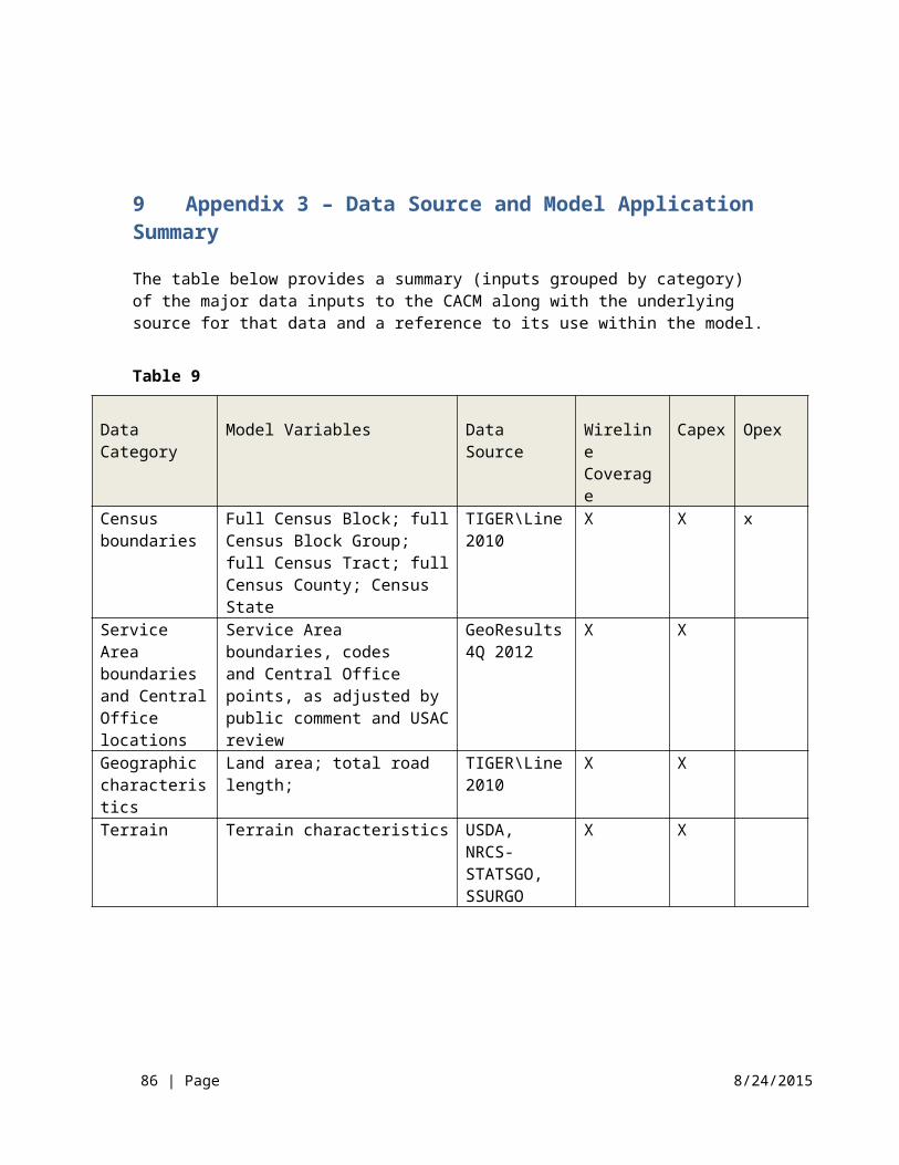
1 2 3 4 5 A B 6 7 8 9 10
Line
Card
Line
Card
Ntw
k Ca
rd
Line
Card
Line
Card
SF/C
PM
SF/C
PM
Ntw
k Ca
rd
Line
Card
Line
Card
Ntw
k Ca
rd
Ntw
k Ca
rd
Notes: IMM slot: 50GbpsIMM cards:
10GigE 8 port >> toward 745010GigE 4 Port >> IOFup to 4 to 1 concentration
SF/CPM: 500GbpsSF - Switch FabricCPM - Control Program Module
Router
Figure 17--Router SchematicIn the GPON network, there are a limited number of aggregation points that constrain broadband speeds. The first aggregation point is the fiber splitter (PFP or FDH). Up to 32 end-user locations can be served off each splitter feeder fiber, with the 32 locations sharing 2.5 Gbps of capacity.54 That means that each location is connected, each connection could have a minimum of 75 Mbps of capacity (i.e., 32 connected locations could all receive 75 Mbps on a single 2.5 Gbps fiber).55 As a result, the maximum per connected location busy hour bandwidth input into CACM should not exceed 75Mbps.
The next aggregation point is the optical line terminal (OLT), where fiber-optic signals from multiple splitter feeder fibers are aggregated and shifted onto a 10 Gbps connection to Ethernet switches and routers (10 Gbps total bandwidth for each OLT). CACM assumes that each OLT can handle as many as 58 active splitter feeder fibers, or 1,856 connected locations (i.e., 58 fibers x 32 locations each assuming all locations passed are connected).56 In other words, the OLT is likely to be the choke-point in the GPON network, where capacity is most limited.57 The CACM inputs are expressed on a “per port or per splitter fiber termination” basis assuming the OLT is fully built out with all ports utilized, adjusted for engineering utilization58. When both splitters and the OLT are fully utilized, each end user is assumed to receive at a minimum 5.4 Mbps of capacity as shown in the following calculation:
54 In fact, 32 end-user locations may have only a fraction of those locations as connected locations, meaning even more capacity per connected location than described in this example.55 Upstream capacity for GPON tends to be one half of downstream.56 Equipment can potentially provide 15 cards with 4 ports each for a total of 60 splitter fibers, but CACM assumes 2 ports are reserved for maintenance and administration purposes.57 As many as 58 2.5 Gbps fibers are backhauled by one 10 Gbps fiber.58 Each of the OLT’s ports is assumed to support up to a maximum of 32 connected locationss per fiber. As such, CACM calculates the number of consumed OLT ports by each splitter by dividing the splitter’s connected locations by 32 and rounding up.
86 | Page 8/24/2015
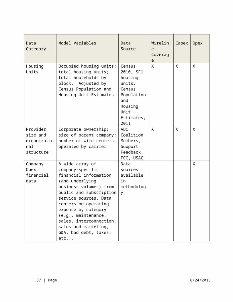
10 Gbps total backhaul from each OLT / 1856 connected locations = 5.4 Mbps per connected location
As shown in the calculation above, the number of connected locations determines the amount of capacity available to each connected location. In denser areas, the splitter is typically fully consumed (i.e., there are 32 end-user locations within 5,000-feet of the splitter). In contrast, in more rural areas it is likely that there will be fewer than 32 end-user locations aggregated onto a single splitter fiber. Thus, in rural areas, where there are more likely to be fewer connected locations per splitter fiber, the architecture used in the model would result in more capacity per connected location.
In addition, in smaller service areas, the OLT utilization would not be as high as that found in larger service areas. In other words, service areas with fewer end-user locations, as is often the case in more rural areas, would be more likely to have unused splitter-fiber capacity aggregating at the OLT, leaving more backhaul capacity from the OLT available to each end user.59 The OLT is still likely to be the choke-point in the network, but end-users each would have more capacity.
Regardless, in the most capacity-constrained areas (areas where OLTs are fully utilized: higher density and likely lower cost), each end user is assumed to receive at least 5.4 Mbps of capacity.60 In rural areas, where it is likely to have fewer than 32 connected locations per splitter fiber and some OLTs underutilized (i.e., less than 58 splitters connected to every OLT), each connected location can have many times this 5.4 Mbps capacity by default, with the exact amount determined by local conditions.
Further toward the core network, the next set of aggregation points are the Ethernet switches and routers, whose capacities (backplane gigabit capability) increases with the number of connected locations assumed to be on the network. In other words, the CACM captures the need for increased capacity in the Ethernet (backhaul) network in less-costly increments, tied to the number of connected locations. The CACM inputs for Ethernet switches and routers are developed on a “per OLT port” basis assuming that these network nodes will be fully utilized adjusted for engineering fill. As noted, each of the OLT’s ports is assumed to support up to a maximum of 32 connected locations per fiber. As such, CACM calculates the Ethernet switch and router investment triggered by each splitter by dividing the splitter’s connected locations by 32 and rounding up. 59 As noted above, OLTs often aggregate demand from an entire service area; and each OLT can provide service for up to 1,856 end-user locations. Thus even in rural areas, each serving wire center is likely to have more than one OLT’s demand. However, it is likely that each splitter fiber in a rural area has, on average, fewer than 32 connected locations. As such, the maximum capacity per connected location would be higher.60 This corresponds to a busy-hour offered load of 5,400 kbps. This is equivalent to a 5.4 Mbps connection being fully utilized through the entire busy hour. Because not all locations served by a splitter will subscribe, rural areas will have fewer locations per splitter, and not all subscribers will require full speeds at all times, the bandwidth required will be much lower than the subscription speed. Thus, it is reasonable for a network offering speeds of 10 Mbps or higher to have a busy hour offered load less than 5.4 Mbps.
87 | Page 8/24/2015

In summary, given the network sizing at each of these aggregation points, and the likely range of reasonable take rates, the modeled network provides much more than 5.4 Mbps of capacity per connected location in rural areas.
14.1. Impact of Bandwidth growth on Broadband Network Equipment CapacitiesAs stated above, CACM has more capacity than needed for the 10/1 service that carriers are required to offer pursuant to the December 2014 Connect America Order.
In prior versions of the CACM, given that the network was configured for capacities greater than the supported service definition, there was no logic to capture the impact of increased busy hour loads. This has been addressed in the latest input files released.
Within the CAPEX input workbook, the investment in the OLTs, Ethernet Switches, and Broadband Routers are all triggered by the number of OLT ports consumed by the terminating Splitter fibers. That is, the OLT, Ethernet Switch, and Broadband Router are unitized on a per OLT port basis, where each port can support up to 32 connected locations from each splitter fiber. As such, for every 32 connected locations of splitter demand (referred to in the CACM methodology as the Node2 demand), CACM adds an increment of investment for these three components.
As described above the OLT acts as the throttle point by providing a maximum of 5400 kbps busy-hour load per connected location or 172Mbps per splitter fiber. The new input files increment the investment of the OLT, Ethernet Switch, and Broadband Router based on the modeled demand that is calculated at each fiber splitter (i.e., Node2). The total bandwidth at fiber splitter is calculated by multiplying the bandwidth per connected location by the take rate at each fiber splitter/Node 2. The CACM compares that aggregate demand to the maximum supported demand of 172Mbps per splitter fiber. Where busy hour load increases and causes the aggregated demand to exceed the capacity of the OLT, the CACM now adds additional cost to account for additional OLT and backhaul capacity.
As an example, if a Fiber Splitter / Node2 location has exactly 32 connected locations (i.e., the take rate times the number of locations leads to a fully utilized splitter with 32 connected locations), there is no incremental cost for any busy-hour load up to 5400 kbps. However, if one were to assume the per-user, busy hour demand had grown to 10,800 kbps, each OLT could handle only half as many fibers (with twice the busy-hour demand each). Therefore, the model calculates additional OLT cost (twice the number of required OLTs), along with added cost for Ethernet Switches, and Broadband Routers In effect, the model has to double the count of OLTs and double the ports consumed on Ethernet Switch, and Broadband Router.
88 | Page 8/24/2015

15 Appendix 9 -- Plant Mix DevelopmentThe following process was used to derive the Plant Mix (i.e., the percentage of Aerial, Buried, and Underground plant) used in the Connect America Cost Model.
15.1. Carrier-Provided Plant Mix Data RequestAs part of the Plant Mix development process, three price cap providers with multi-state operations provided plant mix information in the states in which they operated.61 In short, Plant Mix information was provided by- State- Type of plant – Distribution, Feeder, Inter-Office (IOF)- Density of Area – Rural, Suburban, UrbanSubsequently, a fourth price cap carrier operating in one state provided proposed plant mix values in the same format, which have been incorporated as default values in the plant mix input tables in CACM.
The layout of the data provided is shown below. The following values shown in the table are for illustrative purposes only.
CostFam>>State Density Aerial Buried Underground Aerial Buried Underground Aerial Buried Underground* Rural 50.0% 50.0% 0.0% 45.0% 53.0% 2.0% 45.0% 53.0% 2.0%* Suburban 40.0% 58.0% 2.0% 35.0% 40.0% 25.0% 35.0% 40.0% 25.0%* Urban 30.0% 65.0% 5.0% 20.0% 20.0% 60.0% 20.0% 20.0% 60.0%
DIST Feeder IOF
Figure 18--Data Layout
15.2. Methods
1. Data Validation a. Example -- did the percentages sum to 1 for each Type of Plant?
2. Calculation of Averages for each state where data was submitteda. Averaged submitted values by Density and Type of Plant for those
states where more than one provider submitted data. NB, values showing no decimal places were likely result of operator(s) in a state submitting data without decimal precision.
b. For those states where no state-level data were submitted, averaged values across all states by Density and Type of Plant to develop national averages
3. Compiled into the CACM input table
61 The original plant mix values were publically filed in August 2011 and have been subsequently updated since that time.
89 | Page 8/24/2015
16 Appendix 10 -- Take Rate Impacts to Network Sizing and Cost UnitizationThe business and residential take rate inputs can impact CACM in two ways. First, they can impact how components of the modeled network are sized. Second, they can impact how the total investment and resulting costs are unitized. For purposes of this discussion, “take rate” refers to the percentage of homes or businesses that are connected to the network; it does not refer to the customer subscription levels. With respect to network sizing, some components of the modeled network are impacted by the take rate values. In other words, they are sized based upon connected locations. Other components of the modeled network are not impacted by take rate. These components are sized by total locations.
Take rate’s impact on network sizing can vary based upon the Network Topology used. Under the CACM FTTp network, the black text network components (rows 5-14) in the figure below: NID/Drop, OLT, Eswitch, Router, and cVoip are impacted by take rate. This means that the input values in the business and residential take rate tables will impact how these components are sized and the corresponding
90 | Page 8/24/2015

investment.
After the total network investment is calculated, the unitization is then applied (rows 18, 19 in this example). Note how unitization impacts how the Total Investment is unitized. Although not shown, Total Cost is handled in the same way.
In summary, the take rate values will impact the total investment in the network. The unitization will only impact the per unit investment or cost which is derived from the total investment. Within CACM’s support model, a unitization toggle setting of “No Take Rate Demand” (locations passed) would generate results based on an investment per location value shown in the illustration above with the corresponding take rate value. If the unitization toggle setting is set to “Take Rate Demand” (connected locations) the report would generate results based on an investment per unit take value shown in the illustration above with the corresponding take rate value.
91 | Page 8/24/2015

For clarity, the formulas used in calculating this example are shown below.
The unitization toggle is available to the user when running a report such as a Support Model Detail report. This toggle is available to a user from the CACM home page by selecting the Reporting button. Below is a screen capture showing the “Unitize Cost By” toggle. The toggle allows a user to select “Take Rate Demand” or “No Take Rate Demand” as displayed below.
92 | Page 8/24/2015

By default, version 4.1.1 and subsequent versions of the CAM uses No TakeRate demand.
93 | Page 8/24/2015

17 Document Revisions
5/22/2013Updated for version 3.1.26/5/2013Updated for version 3.1.3, coverage derivation changes and modification to table 3.6/20/2013Clarified application of middle mile sharing. Clarified category breakpoints for urban and suburbanUpdated support model parameter definitions, removed Monthly Support Cap. Added fn, per User Guide.Updated Broadband Network Equipment Capacities section
Updated Capex table definition per User Guide 8/27/2013Updated for version 3.2Updated bandwidth values, removed reference to clear-channel to reduce confusion with TDMUpdated figure 11, figure 3, 10, 14Fixed caption figure 13Removed abbreviation FST to minimize confusion between Fiber Service Terminal and Fiber Splitter Terminal. Added section to address Middle Mile undersea.Added section for Plant Mix development.Updated Figure numbering. Clarified presence of DSLAM.Added footnote, page 29 to clarify the role of density in CAPEX and OPEX.Expanded section 9.3 to include derivation of percentage use factors, removed Mark With Provider from field description.9/15/2013Updated description of broadband coverage development.
94 | Page 8/24/2015

Updated description of bandwidth table.12/1/2013Updated section 3.2 to describe new placement methodsUpdated section 5.2.3.7 to cover terrain modificationsUpdated section 9 to cover new Middle Mile methodsAdded section 5.2.3.5 to cover engineering rulesUpdated table definitions for new workbooks-PlantMixBuried and StateSpecificCapex; mirror User Guide3/4/14Removed TSPO disclaimerUpdated coverage dates and NBM vintage (Table 2 and Table 9)Updated table 9 to remove coverage vintage dates not consistent with other sections of Methodology, added SSURGO as terrain inputs sourceUpdated Appendix 7 to update sharing table illustrations, consistent with current CAPEXUpdated figure 13 to remove coverage vintage dates not consistent with other section of Methodology. Added in new tablesAdded Appendix 10.4/11/14Updated for version 4.1.112/18/14Updated for version 4.2Updated coverage discussionAdded clarifications as to versionsAdded clarification of road types used in model
8/15/20015Updated for ACM version 1.1Updated coverage discussionUpdated data sources corresponding to coverage change (from NBM to FCC Form 477)
95 | Page 8/24/2015