introduction - math.purdue.edumdd/webpapers/invariants-of-almost... · quasi-representations of...
TRANSCRIPT

QUASI-REPRESENTATIONS OF SURFACE GROUPS
JOSE R. CARRION AND MARIUS DADARLAT
Abstract. By a quasi-representation of a group G we mean an ap-proximately multiplicative map of G to the unitary group of a unitalC∗-algebra. A quasi-representation induces a partially defined map atthe level K-theory.
In the early 90s Exel and Loring associated two invariants to almost-commuting pairs of unitary matrices u and v: one a K-theoretic in-variant, which may be regarded as the image of the Bott element inK0(C(T2)) under a map induced by quasi-representation of Z2 in U(n);the other is the winding number in C \ 0 of the closed path t 7→det(tvu+(1− t)uv). The so-called Exel-Loring formula states that thesetwo invariants coincide if ‖uv − vu‖ is sufficiently small.
A generalization of the Exel-Loring formula for quasi-representationsof a surface group taking values U(n) in was given by the second-namedauthor. Here we further extend this formula for quasi-representations ofa surface group taking values in the unitary group of a tracial unitalC∗-algebra.
1. Introduction
Let G be a discrete countable group. In [3, 4] the second-named authorstudied the question of how deformations of the group G (or of the groupC∗-algebra C∗(G)) into the unitary group of a (unital) C∗-algebra A act onthe K-theory of the algebras `1(G) and C∗(G). By a deformation we meanan almost-multiplicative map, a quasi-representation, which we will defineprecisely in a moment. Often, matrix-valued multiplicative maps are inade-quate for detecting the K-theory of the aforementioned group algebras. Infact, if a countable, discrete, torsion free group G satisfies the Baum-Connesconjecture, a unital finite dimensional representation π : C∗(G) → Mr(C)induces the map r · ι∗ on K0(C∗(G)), where ι is the trivial representationof G (see [3, Proposition 3.2]). It turns out that almost-multiplicative mapsdetect K-theory quite well for large classes of groups: one can interpolateany group homomorphism of K0(C∗(G)) to Z on large swaths of K0(C∗(G))using quasi-representations (see [3, Theorem 3.3]).
Knowing that quasi-representations may be used to detect K-theory, weturn to how it is that they act. An index theorem of Connes, Gromov andMoscovici in [2] is very relevant to this topic, in the following context. LetM be a closed Riemannian manifold with fundamental group G and let D
Date: July 13, 2012. (Draft.)M.D. was partially supported by NSF grant #DMS–1101305.
1

2 JOSE R. CARRION AND MARIUS DADARLAT
be an elliptic pseudo-differential operator on M . The equivariant index ofD is an element of K0(`1(G)). Connes, Gromov and Moscovici showed thatthe push-forward of the equivariant index of D under a quasi-representationof G coming from parallel transport in an almost-flat bundle E over M isequal to the index of D twisted by E.
At around the same time, Exel and Loring studied two invariants associ-ated to pairs of almost-commuting scalar unitary matrices u, v ∈ U(r). Oneis a K-theory invariant, which may be regarded as the push-forward of theBott element β in theK0-group of C(T2) ∼= C∗(Z2) by a quasi-representationof Z2 into the unitary group U(r). The Exel-Loring formula proved in [6]states that this invariant equals the winding number in C \ 0 of the patht 7→ det
((1−t)uv+tvu
). An extension of this formula for almost commuting
unitaries in a C∗-algebra of tracial rank one is due to to H. Lin and playsan important role in the classification theory of amenable C∗-algebras. In adifferent direction, the Exel-Loring formula was generalized in [4] to finitedimensional quasi-representations of a surface group using a variant of theindex theorem of [2].
In [4], the second-named author used the Mishchenko-Fomenko index the-orem to give a new proof and a generalization of the index theorem ofConnes, Gromov and Moscovici that allows C∗-algebra coefficients. In thispaper we use this generalization to address the question of how a quasi-representation π of a surface group in the unitary group of a tracial C∗-algebra acts at the level of K-theory. We extend the Exel-Loring formula toa surface group Γg (with canonical generators αi, βi) and coefficients in a uni-tal C∗-algebra A with a trace τ . Briefly, writing K0(`1(Γg)) ∼= Z[ι]⊕Zµ[Σg]we have
τ(µ[Σg]
)=
1
2πiτ
(log
( g∏
i=1
[π(αi), π(βi)
])),
where [Σg] is the fundamental class in K-homology of the genus g surfaceΣg and µ : K0(Σg) → K0(`1(G)) is the `1-version of the assembly map ofLafforgue. For a complete statement see Theorem 2.6. In the proof we makeuse of Chern-Weil theory for connections on Hilbert A-module bundles asdeveloped by Schick [12] and the de la Harpe-Skandalis determinant [5] tocalculate the first Chern class of an almost-flat Hilbert module C∗-bundleassociated to a quasi-representation (Theorem 5.4).
The paper is organized as follows. In Section 2 we define quasi-representationsand the invariants we are interested in, and state out main result, Theo-rem 2.6. The invariants make use of the Mishchenko line bundle, which wediscuss in Section 3. The push-forward of this bundle by a quasi-representationis considered in Section 4. Section 5 contains our main technical result, The-orem 5.4, which computes one of our invariants in terms of the de la Harpe-Skandalis determinant [5]. To obtain the formula given in the main result,we must work with concrete triangulations of oriented surfaces, and this is

QUASI-REPRESENTATIONS OF SURFACE GROUPS 3
contained in Section 6. Assembling these results in Section 7 yields a proofof Theorem 2.6.
2. The main result
In this section we state our main result. It depends on a result in [4] thatwe revisit. Let us provide some notation and definitions first.
Let G be a discrete countable group and A a unital C∗-algebra.
Definition 2.1. Let ε > 0 and let F be a finite subset of G. An (F , ε)-representation of G in U(A) is a function π : G → U(A) such that for alls, t ∈ F we have
• π(1) = 1,• ‖π(s−1)− π(s)∗‖ < ε, and• ‖π(st)− π(s)π(t)‖ < ε.
We refer to the second condition by saying that π is (F , ε)-multiplicative.Let us note that the second condition follows from the other two if weassume that F is symmetric, i.e. F = F−1. A quasi-representation is an(F , ε)-representation where F and ε are not necessarily specified.
A quasi-representation π : G → U(A) induces a map (also denoted π) ofthe Banach algebra `1(G) to A by
∑λss 7→
∑λsπ(s). This map is a unital
linear contraction. We also write π for the extension of π to matrix algebrasover `1(G).
2.2. Pushing-forward via quasi-representations. A group homomor-phism π : G → U(A) induces a map π∗ : K0(`1(G)) → K0(A) (via its Ba-nach algebra extension). We think of a quasi-representation π as induc-ing a partially defined map π] at the level of K-theory, in the followingsense. If e is an idempotent in some matrix algebra over `1(G) such that‖π(e) − π(e)2‖ < 1/4, then the spectrum of π(e) is disjoint from the lineRe z = 1/2. Writing χ for the characteristic function of Re z > 1/2, itfollows that χ(π(e)) is a idempotent and we set
π](e) =[χ(π(e))
]∈ K0(A).
For an element x in K0(`1(G)), we make a choice of idempotents e0 and e1 insome matrix algebra over `1(G) such that x = [e0]−[e1]. If ‖π(ei)−π(ei)
2‖ <1/4 for i ∈ 0, 1, write π](x) = π](e0)− π](e1). The choice of idempotentsis largely inconsequential: given two choices of representatives one finds thatif π is multiplicative enough, then both choices yield the same element ofK0(A).
Of course, the more multiplicative π is, the more elements of K0(`1(G))we can push-forward into K0(A).

4 JOSE R. CARRION AND MARIUS DADARLAT
2.3. An index theorem. Fix a closed oriented Riemannian surface M andlet G be its fundamental group. Fix also a unital C∗-algebra A with a tra-cial state τ . Write K0(M) for KK(C(M),C). Because the assembly mapµ : K0(M)→ K0(`1(G)) is known to be an isomorphism in this case [9], wehave
K0(`1(G)) ∼= Z[1]⊕ Zµ[M ]
where [M ] is the fundamental class of M in K0(M) [1, Lemma 7.9]. Sincewe are interested in how a quasi-representation of G acts on K0(`1(G)),we would like to study push-forward of the generator µ[M ] by a quasi-representation.
2.3.1. Let M be a closed connected orientable manifold with fundamentalgroup G. Consider the universal cover M → M and the diagonal action
of G on M × `1(G) giving rise to the so-called Mishchenko line bundle `,
M ×G `1(G) → G. We will discuss it in more detail in Section 3, where wewill give a description of it as the class of a specific idempotent e in somematrix algebra over C(M)⊗ `1(G).
If π is a quasi-representation of G in U(A), then idC(M)⊗π is an almost-
multiplicative unital linear contraction on C(M) ⊗ `1(G) with values inC(M) ⊗ A. Assuming that π is sufficiently multiplicative, we may definethe push-forward of the idempotent e by idC(M)⊗π, just as in 2.2. We set
`π := (idC(M)⊗π)](`) := (idC(M)⊗π)](e) ∈ K0(C(M)⊗A).
Let D be an elliptic operator on Mn and let µ[D] ∈ K0(`1(G)) be its imageunder the assembly map. Let q0 and q1 be idempotents in some matrixalgebra over `1(G) such that µ[D] = [q0]−[q1] and write π](µ[D]) := π](q0)−π](q1). By [4, Corollary 3.8], if π : G→ A is sufficiently multiplicative, then
(1) τ(π](µ[D]) = (−1)n(n+1)/2⟨(p! ch(σ(D))∪Td(TM⊗C)∪chτ (`π), [M ]
⟩,
where p : TM →M is the canonical projection, ch(σ(D)) is the Chern char-acter of the symbol of D, Td(TCM) is the Todd class of the complexi-fied tangent bundle, and [M ] is the fundamental homology class of M . Set
α = (−1)n(n+1)/2(p!ch(σ(D)) ∪ Td(TM ⊗ C). Then (1) becomes
τ(π](µ[D]) =⟨α ∪ chτ (`π), [M ]
⟩=⟨
chτ (`π), α ∩ [M ]⟩,
On the other hand, it follows from the Atiyah-Singer index theorem thatthe Chern character in homology ch : K0(M)→ H∗(M ;Q) is given by
ch[D] =((−1)n(n+1)/2p! ch(σ(D)) ∪ Td(TCM)
)∩ [M ] = α ∩ [M ].
It follows that
(2) τ(π](µ[D]) =⟨
chτ (`π), ch[D]⟩
In the case of surfaces this formula specializes to the following statement.

QUASI-REPRESENTATIONS OF SURFACE GROUPS 5
Theorem 2.4 (cf. [4, Corollary 3.8]). Let M be a closed oriented Riemann-ian surface of genus g with fundamental group G. Let q0 and q1 be idempo-tents in some matrix algebra over `1(G) such that µ[M ] = [q0]− [q1]. Thenthere exist a finite subset G of G and ω > 0 satisfying the following.
Let A be a unital C∗-algebra with a tracial state τ and let π : G → U(A)be a (G, ω)-representation. Write π](µ[M ]) := π](q0)− π](q1). Then
τ(π](µ[M ])
)= 〈chτ (`π), [M ]〉.
Here chτ : K0
(C(M) ⊗ A
)→ H2(M,R) is a Chern character associated
to τ (see Section 5), and [M ] ∈ H2(M,R) is the fundamental class of M .
Proof. Given another pair of idempotents q′0, q′1 in some matrix algebra over
`1(G) such that µ[M ] = [q′0] − [q′1], there is an ω0 > 0 such that if 0 <ω < ω0, then for any (G, ω)-representation π we have π](q0) − π](q1) =π](q
′0)− π](q′1). We are therefore free to prove the theorem for a convenient
choice of idempotents.It is known that the fundamental class of M in K0(M) coincides with
[∂g] + (g− 1)[ι] where ∂g is the Dolbeault operator on M and ι : C(M)→ Cis a character (see [1, Lemma 7.9]). Let e0, e1, f0, f1 be idempotents in somematrix algebra over `1(G) such that
µ[∂g] = [e0]− [e1] and µ[ι] = [f0]− [f1].
(This gives an obvious choice of idempotents q′0 and q′1 in some matrixalgebra over `1(G) so that µ[M ] = [q′0]− [q′1].) We want to prove that
τ(π](µ(z))
)= 〈chτ (`π), ch(z)〉
for z = [M ] ∈ K0(M). Because of the additivity of this last equation, thefact that [M ] = [∂g] + (g − 1)[ι], and (2), it is enough to prove that
(3) τ(π](µ[ι])
)= 〈chτ (`π), ch[ι]〉.
By [4, Corollary 3.5]
τ(π](µ[ι])
)= τ
(〈`π, [ι]⊗ 1A〉
)
We can represent `π by a projection f in matrices over C(M,A). The defi-nition of the Kasparov product implies that
〈[`π], [ι]⊗ 1A〉 = ι∗[f ] = [f(x0)] ∈ K0(A).
On the other hand, the definition of chτ (see [12, Definition 4.1]) impliesthat chτ (f) = τ(f(x0)) + a term in H2(M,R). Since ch[ι] = 1 ∈ H0(M,R),we get
(4) 〈chτ (f), ch[ι]〉 = τ(f(x0)).

6 JOSE R. CARRION AND MARIUS DADARLAT
2.5. Statement of the main result. We will often write Σg for the closedoriented surface of genus g and Γg for its fundamental group. It is well knownthat Γg has a standard presentation
Γg =
⟨α1, β1, . . . , αg, βg
∣∣∣∣g∏
i=1
[αi, βi]
⟩,
where we write [α, β] for the multiplicative commutator αβα−1β−1.Our main result is the following.
Theorem 2.6. Let g ≥ 1 be an integer and let q0 and q1 be idempotents insome matrix algebra over `1(Γg) such that µ[Σg] = [q0]− [q1] ∈ K0(`1(Γg)).There exists ε0 > 0 and a finite subset F0 of Γg such that for every 0 < ε < ε0
and every finite subset F ⊇ F0 of Γg the following holds.If A is a unital C∗-algebra with a trace τ and π : Γg → U(A) is an (F , ε)-
representation, then
(5) τ(π](µ[Σg])
)=
1
2πiτ
(log
( g∏
i=1
[π(αi), π(βi)
])),
where π](µ[Σg]) := π](q0)− π](q1).
The rest of the paper is devoted to the proof.
Remark 2.7. The case g = 1 recovers the Exel-Loring formula as well as itsextension by H. Lin [10] for C∗-algebras of tracial rank one. Lin’s strategywas a reduction to the finite-dimensional case of [6] using approximationtechniques.
The following proposition says that we may associate quasi-representationswith unitaries that nearly satisfy the group relation. The proof is in Sec-tion 7.
Proposition 2.8. For every ε > 0 and every finite subset F of Γg there is aδ > 0 such that if A is a unital C∗-algebra with a trace τ and u1, v1, ..., ug, vgare unitaries in A satisfying
∥∥∥∥g∏
i=1
[ui, vi]− 1
∥∥∥∥ < δ,
then there exists an (F , ε)-representation π : Γg → U(A) with π(αi) = uiand π(βi) = vi, for all i ∈ 1, . . . , g.Example. To revisit a classic example, consider the noncommutative 2-torus Aθ, regarded as the universal C∗-algebra generated by unitaries u andv with [v, u] = e2πiθ · 1. This is a tracial unital C∗-algebra. If θ is smallenough, we may apply Proposition 2.8 and Theorem 2.6 to obtain
τ(π](β)) =1
2πiτ(log e−2πiθ) = −θ
where β ∈ K0(C(T2)) is the Bott element, τ is a unital trace of Aθ, andπ : Z2 → U(Aθ) is a quasi-representation obtained from Proposition 2.8.

QUASI-REPRESENTATIONS OF SURFACE GROUPS 7
3. The Mishchenko line bundle
Recall our setup: M is a closed oriented surface with fundamental group
G and universal cover p : M → M . In this section we give a picture of theMishchenko line bundle that will enable us to explicitly describe its push-forward by a quasi-representation.
The Mishchenko line bundle is the bundle M ×G `1(G) → M , obtained
from M × `1(G) by passing to the quotient with respect to the diagonalaction of G. We write ` for its class in K0(C(M)⊗ `1(G)).
3.1. Triangulations and the edge-path group. We adapt a constructionfound in the appendix of [11]. It is convenient to work with a triangulation
Λ of M . Let Λ(0) = x0, . . . , xN−1 be the 0-skeleton of Λ and Λ(1) be the1-skeleton. To each edge we assign an element of G as follows. Fix a rootvertex x0 and a maximal (spanning) tree T in Λ. Let γi be the unique pathalong T from x0 to xi, and for two adjacent vertices xi and xj let xixj be the(directed) edge from xi to xj . For two such adjacent vertices, write sij ∈ Gfor the class of the loop γi ∗ xixj ∗ γ−1
j .
Let F be the (finite) set sij. For example, if M = T2 so that G = Z2 =〈α, β : [α, β] = 1〉, we have F = 1, α±1, β±1, (αβ)±1 for the triangulationand tree pictured in Figure 3 (on page 19)
Definition 3.2. For a vertex xik in a 2-simplex σ = 〈xi0 , xi1 , xi2〉 of Λ,define the dual cell block to xik
Uσik :=
2∑
l=0
tlxil : tl ≥ 0,
2∑
l=0
tl = 1, and tik ≥ tl for all l
.
Define the dual cell to the vertex xi ∈ Λ(0) by
Ui = ∪Uσi : xi ∈ σ.Let Uσij = Uσi ∩ Uσj etc. (See Figure 1.)
Since p : M → M is a covering space of M , we may fix an open cover ofM such that for every element V of this cover, p−1(V ) is a disjoint union of
open subsets of M , each of which is mapped homeomorphically onto V byp. We require that Λ be fine enough so that every dual cell Ui is containedin some element of this cover.
Lemma 3.3. The Mishchenko line bundle M ×G `1(G)→M is isomorphicto the bundle E obtained from the disjoint union
⊔Ui× `1(G) by identifying
(x, a) with (x, sija) whenever x ∈ Ui ∩ Uj.
Proof. Lift x0 to a vertex x0 in M . By the unique path-lifting property,every path γi lifts (uniquely) to a path γi from x0 to a lift xi of xi. In this
way lift T to a tree T in M . Each Ui also lifts to a dual cell to xi, denoted
Ui, which p maps homeomorphically onto Ui.
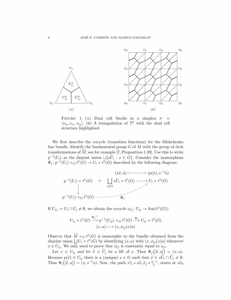
8 JOSE R. CARRION AND MARIUS DADARLAT
vi0
vi1
vi2
Uσi0
Uσi1
Uσi2
(a)
v0 v1 v2 v0
v0 v1 v2 v0
v3
v4
v3
v4
(b)
Figure 1. (a) Dual cell blocks in a simplex σ =〈vi0 , vi1 , vi2〉. (b) A triangulation of T2 with the dual cellstructure highlighted.
We first describe the cocycle (transition functions) for the Mishchenkoline bundle. Identify the fundamental group G of M with the group of deck
transformations of M ; see for example [7, Proposition 1.39]. Use this to write
p−1(Ui) as the disjoint union tsUi : s ∈ G. Consider the isomorphismΦi : p
−1(Ui)×G `1(G)→ Ui × `1(G) described by the following diagram:
(sx, a) (p(x), s−1a)
p−1(Ui) × `1(G)⊔
s∈GsUi × `1(G) Ui × `1(G)
p−1(Ui) ×G `1(G) Φi
=
If Uij := Ui ∩ Uj 6= ∅, we obtain the cocycle φij : Uij → Aut(`1(G)):
Uij × `1(G)Φ−1j−→ p−1(Uij)×G `1(G)
Φi−→ Uij × `1(G)
(x, a) 7−→ (x, φij(x)a)
Observe that M ×G `1(G) is isomorphic to the bundle obtained from thedisjoint union
⊔Ui × `1(G) by identifying (x, a) with (x, φij(x)a) whenever
x ∈ Uij . We only need to prove that φij is constantly equal to sij .
Let x ∈ Uij and let x ∈ Uj be a lift of x. Then Φj
([x, a]
)= (x, a).
Because p(x) ∈ Uij there is a (unique) s ∈ G such that x ∈ sUi ∩ Uj 6= ∅.Thus Φi
([x, a]
)= (x, s−1a). Now, the path sγi ∗ sxi xj ∗ γ−1
j , starts at sx0

QUASI-REPRESENTATIONS OF SURFACE GROUPS 9
and ends at x0. Its projection in M is the loop defining sij , so s−1 = sij(see [7, Proposition 1.39], for example). Thus φij(x) = sij .
3.4. The push-forward of the line bundle. We will need an open coverof M , so we dilate the dual cells Ui to obtain one. Let 0 < δ < 1/2 anddefine V σ
i to be the δ-neighborhood of Uσi intersected with σ. As before, setVi =
⋃σ V
σi . Let χi be a partition of unity subordinate to Vi.
By Lemma 3.3 the class of the Mishchenko line bundle in K0(C(M) ⊗`1(G)), denoted earlier by `, corresponds to the class of the projection
e :=∑
i,j
eij ⊗ χ1/2i χ
1/2j ⊗ sij ∈MN (C)⊗ C(M)⊗ `1(G),
where eij are the canonical matrix units of MN (C) and N is the numberof vertices in Λ.
We may fix a pair of idempotents q0 and q1 in some matrix algebra over`1(G) satisfying [q0] − [q1] = µ[M ] ∈ K0(`1(G)). Let ω > 0 be given byTheorem 2.4. (We may assume that ω < 1/4.)
Fix 0 < ε < ω and an (F , ε)-representation π : G → U(A). We recall thefollowing notation from the introduction.
Notation 3.5. For an (F , ε)-representation π : G→ U(A) as above, let
`π := (idC(M)⊗π)](e).
4. Hilbert-module bundles and quasi-representations
As mentioned in the introduction, in [2] a quasi-representation (withscalar values) of the fundamental group of a manifold is associated to an“almost-flat” bundle over the manifold. In this section we instead define acanonical bundle Eπ over M associated with quasi-representation π. Its classin K0(C(M)⊗A) will be the class `π of the push-forward of the Mishchenkoline bundle by π. Our construction will be explicit enough so that we canuse Chern-Weil theory for such bundles to analyze chτ (`π), see [12].
Recall that A is a C∗-algebra with trace τ .
Definition. Let X be a locally compact Hausdorff space. A Hilbert A-module bundle W over X is a topological space W with a projection W → Xsuch that the fiber over each point has the structure of a Hilbert A-moduleV , and with local trivializations W |U ∼−→ U ×V which are fiberwise HilbertA-module isomorphisms.
We should point out that the K0-group of the C∗-algebra C(M) ⊗ Ais isomorphic to the Grothendieck group of isomorphism classes of finitelygenerated projective Hilbert A-module bundles over M . We identify the twogroups.
10 JOSE R. CARRION AND MARIUS DADARLAT
4.1. Constructing bundles. We adapt a construction found in [11].First we define a family of maps uij : Uij → GL(A) satisfying
uji(x) = u−1ij (x), x ∈ Uij ,
uik(x) = uij(x)ujk(x), x ∈ Uijk.
These maps will be then extended to a cocycle defined on the collectionVij.
Following [11] we will find it convenient to fix a partial order o on thevertices of Λ such that the vertices of each simplex form a totally orderedsubset. We then call Λ a locally ordered simplicial complex. One may alwaysassume such an order exists by passing to the first barycentric subdivisionof Λ: if σ1 and σ2 are the barycenters of simplices σ1 and σ2 of Λ, defineσ1 < σ2 if σ1 is a face of σ2.
Consider a simplex σ = 〈xi0 , xi1 , xi2〉 (with vertices written in increasingo-order). Observe that in this case Uσi0 ∩Uσi2 = Uσi0i2 may be described usinga single parameter t1:
Uσi0i2 =
2∑
l=0
tlxil : t0 = t2 =1− t1
2: 0 ≤ t1 ≤ 1/3
.
Define
uσi0i1 = the constant function on Uσi0i1 equal to π(si0i1)
uσi1i2 = the constant function on Uσi1i2 equal to π(si1i2)
uσi0i2(t1) = (1− 3t1)π(si0i2) + 3t1π(si0i1)π(si1i2), 0 ≤ t1 ≤ 1/3.
Define uσi2i0 etc. to be the pointwise inverse of uσi0i2 . For fixed i and j, themaps uσij : Uσij → GL(A) define a map uij : Uij → GL(A). Indeed, if xixj is
a common edge of two simplices σ and σ′, then Uσij ∩ Uσ′
ij is the barycenter
of 〈xi, xj〉, where by definition both uσij and uσ′ij take the value π(sij). By
construction the family uij has the desired properties. (Note that Uijk isthe barycenter of a 2-simplex.)
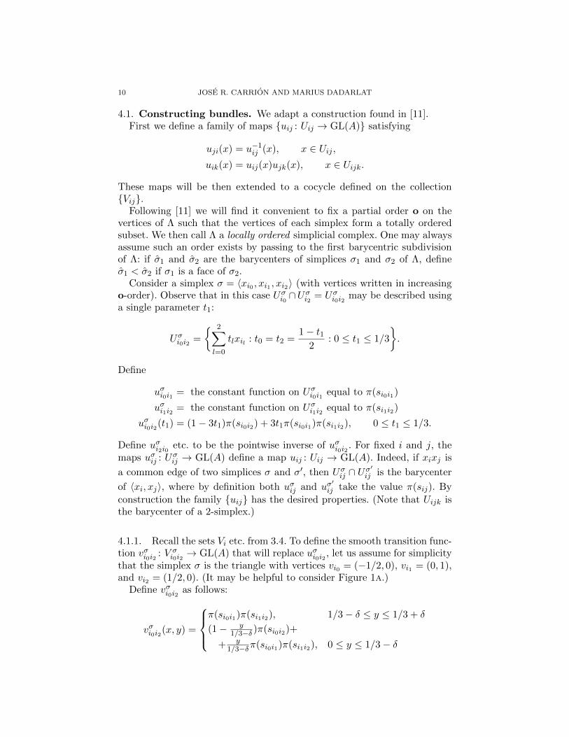
4.1.1. Recall the sets Vi etc. from 3.4. To define the smooth transition func-tion vσi0i2 : V σ
i0i2→ GL(A) that will replace uσi0i2 , let us assume for simplicity
that the simplex σ is the triangle with vertices vi0 = (−1/2, 0), vi1 = (0, 1),and vi2 = (1/2, 0). (It may be helpful to consider Figure 1a.)
Define vσi0i2 as follows:
vσi0i2(x, y) =
π(si0i1)π(si1i2), 1/3− δ ≤ y ≤ 1/3 + δ
(1− y1/3−δ )π(si0i2)+
+ y1/3−δπ(si0i1)π(si1i2), 0 ≤ y ≤ 1/3− δ

QUASI-REPRESENTATIONS OF SURFACE GROUPS 11
(so vσi0i2 is constant along the horizontal segments in Vi0i2). The remainingtwo transition functions remain constant:
vσi0i1 = π(si0i1)
vσi1i2 = π(si1i2)
Again, for fixed i and j the maps vσij : V σij → GL(A) define a map vij : Vij →
GL(A). Since vσi0i2 is constant and equal to π(si0i1)π(si1i2) in Vi0 ∩Vi2 ∩Vi2 ,we indeed obtain a family vij of transition functions.
Definition 4.2. The Hilbert A-module bundle Eπ is constructed from thedisjoint union
⊔Vi ×A by identifying (x, a) with (x, vij(x)a) for x in Vij .
Proposition 4.3. The class of Eπ in K0(C(M)⊗A) coincides with `π, theclass of the push-forward of e by idC(M)⊗π (see 3.4).
Proof. The bundle Eπ is a quotient of⊔Vi ×A and from its definition it is
clear that for each i the quotient map is injective on Vi×A. The restriction ofthe quotient map to Vi×A has an inverse, call it ψi, and ψi is a trivializationof Eπ|Vi . Recalling that N is the number of vertices in Λ (which is the sameas the number of sets Vi in the cover), we define an isometric embedding
θ : Eπ →M ×AN
[x, a] 7→(χ
1/2i (x)ψi([x, a])
)N−1
i=0.
Let eπ : M →MN (A) be the function
x 7→∑
i,j
eij ⊗ χ1/2i (x)χ
1/2j (x)vij(x).
Because ψiψ−1j (x, a) = (x, vij(x)a) for x ∈ Vij , it is easy to check that eπ(x)
is the matrix representing the orthogonal projection of AN onto θ(Eπ|x). Inthis way we see that [Eπ] = [eπ] ∈ K0(C(M)⊗A).
Since F = sij and π is an (F , ε)-representation, it follows immediatelythat the transition functions vij satisfy ‖vij(x)− π(sij)‖ < ε for all x ∈ Vij .Thus
‖eπ − (1⊗ π)(e)‖ =
∥∥∥∥eπ −∑
i,j
eij ⊗ χ1/2i χ
1/2j π(sij)
∥∥∥∥ < ε
as well. Recall that `π is obtained by perturbing (1 ⊗ π)(e) to a projectionusing functional calculus and then taking its K0-class (see 2.2). The previousestimate shows that this class must be [eπ].
Remark 4.4. The previous proposition shows that the class [Eπ] is inde-pendent of the order o on the vertices of Λ0.
4.5. Connections arising from transition functions. We now define acanonical connection on Eπ associated with the family vij of transitionfunctions. This connection will be used in the proof of Theorem 5.4.

12 JOSE R. CARRION AND MARIUS DADARLAT
4.5.1. The smooth sections Γ(Eπ) of Eπ may be identified with
(si) ∈⊕
i
Ω0(Vi, Eπ) : sj = vjisi on Vij.
Let ∇i : Ω0(Vi, A)→ Ω1(Vi, A) be given by
∇i(s) = ds+ ωis ∀s ∈ Ω0(Vi, A),
where
ωi =∑
k
χkv−1ki dvki.
Notice that vki ∈ Ω0(Vik,GL(A)) and so ωi may be regarded as an A-valued1-form on Vi, which can be multiplied fiberwise by the values of the sections.
We define a connection ∇ on Eπ by
∇(si) = (∇isi).That ∇ takes values in Ω1(M,Eπ) follows from a straightforward computa-tion verifying
∇jsj = vji∇isi.It is just as straightforward to verify that ∇ is A-linear and satisfies theLeibniz rule.
4.5.2. Define Ωi = dωi+ωi∧ωi ∈ Ω2(Vi, A). One checks that Ωi = v−1ji Ωjvji
and so (Ωi) defines an element Ω of Ω2(M,EndA(Eπ)). This is nothing butthe curvature of ∇ (see [12, Proposition 3.8]).
5. The Chern character
In this section we prove our main technical result, Theorem 2.6. It com-putes the trace of the push-forward of µ[M ] in terms of the de la Harpe-Skandalis determinant by using that the cocycle conditions almost hold forthe elements π(sij),
5.1. The de la Harpe-Skandalis determinant. The de la Harpe-Skandalisdeterminant [5] appears in our formula below. Let us recall the definition.Write GL∞(A) for the (algebraic) inductive limit of (GLn(A))n≥1 with stan-dard inclusions. For a piecewise smooth path ξ : [t1, t2]→ GL∞(A), define
∆τ (ξ) =1
2πiτ
( t2∫
t1
ξ′(t)ξ(t)−1dt
)=
1
2πi
t2∫
t1
τ(ξ′(t)ξ(t)−1)dt.
We will make use of some of the properties of ∆τ stated below.
Lemma 5.2 (cf. Lemme 1 of [5]).
(1) Let ξ1, ξ2 : [t1, t2] → GL0∞(A) be two paths and ξ be their pointwise
product. Then ∆τ (ξ) = ∆τ (ξ1) + ∆τ (ξ2).
QUASI-REPRESENTATIONS OF SURFACE GROUPS 13
(2) Let ξ : [t1, t2] → GL0∞(A) be a path with ‖ξ(t) − 1‖ < 1 for all t.
Then
2πi · ∆τ (ξ) = τ(log ξ(t2)
)− τ(log ξ(t1)
).
(3) The integral ∆τ (ξ) is left invariant under a fixed-end-point homotopyof ξ.
5.3. The Chern character on K0(C(M) ⊗ A). Assume τ is a trace onA. Then τ induces a map on Ω2(Vi,EndA(Eπ|Vi)) and by the trace propertyτ(Ωi) = τ(Ωj) on Vij . We obtain in this way a globally defined form τ(Ω) ∈Ω2(M,C).
Since the fibers of our bundle are all equal to A, and our manifold is 2-dimensional, the definition of the Chern character associated with τ (from[12, Definition 4.1], but we have included a normalization coefficient) reducesto
(6) chτ (`π) = τ
(exp
(iΩ
2π
))= τ
( ∞∑
k=0
iΩ/2π ∧ · · · ∧ iΩ/2πk!
)=
= τ
(iΩ
2π
)∈ Ω2(M,C).
This is a closed form whose cohomology class does not depend on the choiceof the connection ∇ (see [12, Lemma 4.2]).
A few remarks are in order before stating the next result.Because Λ is a locally ordered simplicial complex (recall the partial order
o from 4.1), every 2-simplex σ may be written uniquely as 〈xi, xj , xk〉 withthe vertices written in increasing o-order. Whenever we write a simplex inthis way it is implicit that the vertices are written in increasing o-order. Wemay write σ for σ along with this order.
The orientation [M ] induces an orientation of the boundary of the dual cellUi and in particular of the segment Uσik. Let s(σ) = 0 if the initial endpoint ofUσik under this orientation is the barycenter of σ, and let s(σ) = 1 otherwise.
Theorem 5.4. For a simplex σ = 〈xi, xj , xk〉 of Λ, let ξσ be the linear path
ξσ(t) = (1− t)π(sik) + tπ(sij)π(sjk), t ∈ [0, 1]
in GL(A). Then
τ(π](µ[M ])
)=∑
σ
(−1)s(σ)∆τ (ξσ),
where the sum ranges over all 2-simplices σ of Λ.
Proof. The path ξσ lies entirely in GL(A) because ‖π(sik)−π(sij)π(sjk)‖ <ε. It follows from Theorem 2.4 (on page 5) and Equation (6) above that
τ(π](µ[M ])
)= 〈chτ (`π), [M ]〉 = − 1
2πi
∫
M
τ(Ω).

14 JOSE R. CARRION AND MARIUS DADARLAT
We compute this integral.First observe that by the trace property of τ we have τ(ωl ∧ ωl) = 0 for
every l. Thus
∫
M
τ(Ω) =∑
l
∫
Ul
τ(Ωl) =∑
l
∫
Ul
τ(dωl + ωl ∧ ωl) =
=∑
l
∫
Ul
τ(dωl) =∑
l
∫
Ul
dτ(ωl) =∑
l
∫
∂Ul
τ(ωl),
where we used Green’s theorem for the last equality and ∂Ul has the orien-tation induced from [M ]. Recall that Ul is the dual cell to vl. Write this asa sum over the 2-simplices of Λ:
∑
l
∫
∂Ul
τ(ωl) =∑
l
∑
σ
∫
(∂Ul)∩σ
τ(ωl) =∑
σ
∑
l
∫
(∂Ul)∩σ
τ(ωl).
Exactly three dual cells meet a 2-simplex σ = 〈xi, xj , xk〉—Ui, Uj , and Uk—so for each simplex there are three integrals we need to account for. Let ustreat each of these in turn.
The definition of the connection forms (see 4.5.1) implies that ωi restrictedto σ equals
ωi = χkv−1ki dvki + χjv
−1ji dvji = χkv
−1ki dvki,
where the last equality follows from the fact that vji is constant. Now, (∂Ui)∩σ is the union of the two segments Uσij and Uσik. Observe that vik is constantly
equal to π(sij)π(sjk) on Vi∩Vj ∩Vk (see 4.1.1). Since Uσij ∩Vk ⊆ Vi∩Vj ∩Vkand χk vanishes outside Vk, we get
∫
(∂Ui)∩σ
τ(ωi) =
∫
Uσij
τ(χkv−1ki dvki) +
∫
Uσik
τ(χkv−1ki dvki) =
∫
Uσik
τ(χkv−1ki dvki).
The second integral∫
(∂Uj)∩σ τ(ωj) vanishes. This is because vij and vjkare constant and so
ωj = χiv−1ij dvij + χkv
−1kj dvkj = 0.
The third integral may be calculated just as the first, with the roles of iand k reversed. We obtain
∫
(∂Uk)∩σ
τ(ωk) =
∫
Uσki
τ(χiv−1ik dvik).

QUASI-REPRESENTATIONS OF SURFACE GROUPS 15
Combining the three integrals we get
∑
σ
∑
l
∫
(∂Ul)∩σ
τ(ωl) =∑
σ
( ∫
Uσik
τ(χkv−1ki dvki) +
∫
Uσki
τ(χiv−1ik dvik)
)=
=∑
σ
∫
Uσik
τ(χkv−1ki dvki − χiv−1
ik dvik),
where the last equality is due to the opposite orientations of the segmentUσik in the preceding two integrals.
It follows from vikvki = 1 that dvik v−1ik + v−1
ki dvki = 0. Therefore, the lastline in the equation above is equal to∑
σ
∫
Uσik
τ(χkv−1ki dvki+χiv
−1ki dvki) =
∑
σ
∫
Uσik
τ(v−1ki dvki) = −
∑
σ
∫
Uσik
τ(v−1ik dvik).
To arrive at the conclusion of the theorem, consider the restriction of vikto the segment Uσik. This is the segment between the barycenter of σ, wherevik takes the value π(sij)π(sjk), and the barycenter of 〈xi, xk〉, where viktakes the value π(sik) (see 4.1.1). Then
∫
Uσik
τ(v−1ki dvki) = (−1)s(σ)2πi · ∆τ (ξσ).
This concludes the proof.
6. Oriented surfaces
For the proof of Theorem 2.6, we will use a convenient triangulation Λg ofthe orientable genus g surface Σg that we proceed to describe. The coveringspace of Σg is the open disc and we may take as a fundamental domain a
regular 4g-gon, call it Σg, drawn in the hyperbolic plane.
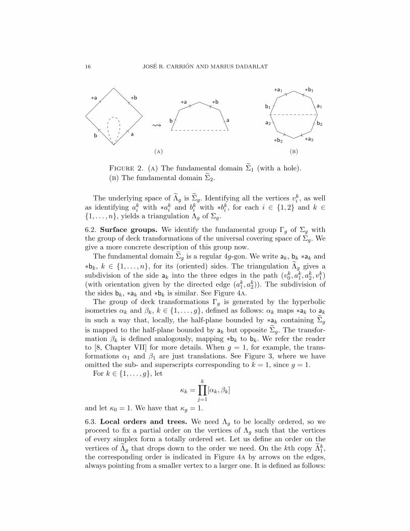
Figure 2 depicts a procedure to obtain Σ2 by gluing together two copies
of Σ1. (We will give a more explicit description of Σg in a moment). It also
illustrates the labeling we use for the (oriented) sides of Σ1 and Σ2. Toobtain Σ1, for example, we identify the side a with ∗a and the side b with∗b. To obtain the double torus Σ2, we identify ak with ∗ak and bk with ∗bkfor k ∈ 1, 2.
6.1. Triangulations. Let us first define a triangulation Λg of the funda-
mental domain Σg. We do this by gluing g triangulated copies of Σ1 to-
gether. Figure 4a on page 20 shows the triangulation for the kth copy of Σ1
(with a hole), call it Λk1. Ignore the labels on the edges and the highlighted
edges for now. The vertex labeling also indicates how to glue Λk1 to Λk−11
and Λk+11 , with addition modulo g. Figure 4b illustrates the result of this
gluing, the end-result being Λg by definition.
16 JOSE R. CARRION AND MARIUS DADARLAT
∗b∗a
b a
a
∗b∗a
b
(a)
a1
∗b1∗a1
b1
a2
∗b2 ∗a2
b2
(b)
Figure 2. (a) The fundamental domain Σ1 (with a hole).
(b) The fundamental domain Σ2.
The underlying space of Λg is Σg. Identifying all the vertices vki , as well
as identifying aki with ∗aki and bki with ∗bki , for each i ∈ 1, 2 and k ∈1, . . . , n, yields a triangulation Λg of Σg.
6.2. Surface groups. We identify the fundamental group Γg of Σg withthe group of deck transformations of the universal covering space of Σg. Wegive a more concrete description of this group now.
The fundamental domain Σg is a regular 4g-gon. We write ak, bk ∗ak and
∗bk, k ∈ 1, . . . , n, for its (oriented) sides. The triangulation Λg gives a
subdivision of the side ak into the three edges in the path (vk0 , ak1, a
k2, v
k1 )
(with orientation given by the directed edge (ak1, ak2)). The subdivision of
the sides bk, ∗ak and ∗bk is similar. See Figure 4a.The group of deck transformations Γg is generated by the hyperbolic
isometries αk and βk, k ∈ 1, . . . , g, defined as follows: αk maps ∗ak to akin such a way that, locally, the half-plane bounded by ∗ak containing Σg
is mapped to the half-plane bounded by ak but opposite Σg. The transfor-mation βk is defined analogously, mapping ∗bk to bk. We refer the readerto [8, Chapter VII] for more details. When g = 1, for example, the trans-formations α1 and β1 are just translations. See Figure 3, where we haveomitted the sub- and superscripts corresponding to k = 1, since g = 1.
For k ∈ 1, . . . , g, let
κk =
k∏
j=1
[αk, βk]
and let κ0 = 1. We have that κg = 1.
6.3. Local orders and trees. We need Λg to be locally ordered, so weproceed to fix a partial order on the vertices of Λg such that the verticesof every simplex form a totally ordered set. Let us define an order on the
vertices of Λg that drops down to the order we need. On the kth copy Λk1,the corresponding order is indicated in Figure 4a by arrows on the edges,always pointing from a smaller vertex to a larger one. It is defined as follows:

QUASI-REPRESENTATIONS OF SURFACE GROUPS 17
• for the “inner” vertices we go “counter-clockwise”: for fixed k ∈1, . . . , g, wki < wkj if i < j, except when k = g and j = 4 (in which
case wg4 = w10 and we already have w1
0 < wik);
• the “inner” vertices are larger than the “outer” ones: wki > vlj , alj ,
blj , ∗alj , ∗blj for all i, j, k and l;
• for the “outer” vertices: vki < alj , blj , ∗alj , ∗blj for all i, j, k and l; for
every k, ak1 < ak2, ∗ak1 < ∗ak2, and similarly for the bkj .
Finally, we will need a spanning tree Tg of Λg, and a lift Tg to the trian-
gulation Λg of the fundamental domain Σg. Again, we define Tg first. It isobtained as the union of the edge between w1
0 and v10 (including those two
vertices) and trees in each copy Σk1. The tree in Σk
1 is depicted in Figure 4aby highlighted (heavier) edges. This drops to a spanning tree Tg of Σg. we
regard these trees as “rooted” at the vertex vk0 .
7. Proof of the main result
This section contains the proof of Theorem 2.6. The proof is split into anumber of lemmas.
To apply Theorem 5.4 we will first compute the group element sij corre-sponding to each edge xixj of Λg , in the sense discussed in 3.1. Equivalently,
we compute group elements corresponding to edges in the cover Λg, keepingin mind that the lifts of any edge of Λg will all correspond to the same groupelement.
A concise way of stating the result of these computations is to label eachedge in Figure 4a with the corresponding group element.
Lemma 7.1. The labels in Figure 4a are correct.
Proof. We carry out the computations in three separate claims.
Claim. An edge of the form akiwkj corresponds to α−1
k ∈ Γg. Similarly, an
edge of the form bkiwkj corresponds to β−1
k ∈ Γg.
Consider akiwkj first. When we add this edge to the forest that is the
union of all the lifts of Tg (that is, translates of Tg), we obtain a uniquepath P between v1
0, our root vertex, and some translate sv10, where s ∈ Γg.
We regard P as directed in the direction of the edge akiwkj that we started
with, so it is a path from sv10 to v1
0. It therefore drops down to a loopin Σg whose class is s−1, the group element we want to compute (see [7,
Proposition 1.39], for example). Now notice that because ∗aki belongs to Tg,
its translate αk(∗aki ) = aki belongs to the translate αkTg of Tg. Thus P is
a path between vk0 and αkvk0 . The corresponding group element is therefore
α−1k . An entirely similar argument applies to the edge bkiw
kj .

18 JOSE R. CARRION AND MARIUS DADARLAT
Claim. Any edge between inner vertices (vertices of the form wki ) corre-sponds to 1 ∈ Γg. The edges ak1a
k2, bk1b
k2, ∗ak1∗ak2, and ∗bk1∗bk2 all correspond
to 1 ∈ Γg.
We proceed as in the previous claim. Any edge between inner vertices is
either in Tg or between two vertices that are in Tg. The associated path we
get is therefore from vk0 to itself. The same is true of the edges bk1bk2 and
∗ak1∗ak2. It follows that the corresponding group element is 1. Since ak1ak2 and
∗ak1∗ak2 are both lifts of the same edge, they correspond to the same element.Similarly, ∗bk1∗bk2 corresponds to 1.
Claim. An edge that is incident to vki and to a vertex z in the tree Tgcorresponds to the element s ∈ Γg such that v1
0 = svki . (The edge is giventhe orientation induced by the order on the vertices, as usual.) For k ∈1, . . . , g,
v10 = κk−1 · vk0v1
0 = κk−1αkβkα−1k · vk1
v10 = κk−1αkβk · vk2v1
0 = κk−1αk · vk3
(Recall that κk is the product of commutators [α1, β1][α2, β2] · · · [αk, βk] fork ∈ 1, . . . , g, and that κ0 = 1.)
Observe that, because of how the order was defined, vki < z always holds.
When we add the edge vki z to the tree Tg we obtain a path from vki to v10.
(See Figure 4, but keep in mind that in the case k = 1 the edge v10w
10 belongs
to the tree.) It follows that the corresponding element is the s ∈ Γg such
that v10 = svki .
To compute these elements s we argue by induction on k. Assume k = 1.We observe that
v14
β−117−→ v1
1
α−117−→ v1
2β17−→ v1
3α17−→ v1
0.
Indeed, from the definition (see 6.2) we see that the transformation α1 takesv1
3 to v10—think of the side ∗a1 = (v1
3, ∗a11, ∗a1
2, v12) being mapped to the side
a1 = (v10, a
11, a
12, v
11): the vertex ∗a1
1 is mapped to a11 and so v1
3 is mappedto v1
0. We also see from 6.2 and Figure 4a that β1 maps v12 to v1
3, and so
v10 = α1β1 · v1
2. A similar argument shows that v10 = α1β1α
−11 · v1
1 and that
v10 = α1β1α
−11 β−1
1 · v14 = κ1 · v1
4.
Assuming the computations hold for k − 1, we prove them for k. In fact,most of the work is already done. The same argument we used for the casek = 1 shows that
vk4β−1k7−→ vk1
α−1k7−→ vk2
βk7−→ vk3αk7−→ vk0 .

QUASI-REPRESENTATIONS OF SURFACE GROUPS 19
v1
v2
v3
v0
w−1 w1
w2
w3
w0
∗a1
∗a2
b1
b2 a2
a1
∗b2
∗b111
1 1
β
αβ
α
β−1
α −1
β−1
α −1
11
β −1
α−1
β
αβαβ
α
αβ
β α
αβ
11
1 1
Figure 3. The triangulation Λ1 of Σ1. Edges are labeledwith the group element associated with the loop they induce.
The inductive hypothesis implies that
κk−1vk0 = κk−1v
k−14 = v1
0,
This ends the proof of the claim.These three claims prove that the labels in Figure 4a are correct.(The labels in Figure 3 also follow from these calculations, but may be
obtained by more straightforward arguments because the generators of Γ1∼=
Z2 may be regarded as shifts in the plane.)
Notation 7.2. For k ∈ 1, . . . , g, let
Fk = α−1k , β−1
k , κk−1, κk−1αk, κk−1αkβk, κk−1αkβkα−1k ,
and notice that the set F = sij considered in section 3.1 is equal to the
union F1 ∪ F−11 ∪ · · · ∪ Fg ∪ F−1
g by Lemma 7.1.
7.3. Choosing quasi-representations. We want to apply Theorem 5.4using the labels obtained in Lemma 7.1 and some convenient choice of aquasi-representation of G in U(A). We begin by proving a slightly strongerversion Proposition 2.8, which guarantees the existence of quasi-representations(under certain conditions). Let us set up some notation first.

20 JOSE R. CARRION AND MARIUS DADARLAT
vk−14 = vk0
vk1
vk2
vk3
vk4 = vk+10
wk−1−1 = wk
−1 = wk+1−1 wk
4 = wk+10wk
0 = wk−14
wk1
wk2
wk3
bk1
bk2
∗ak1
∗ak2∗bk2
∗bk1
ak2
ak1
1
1 1
1
κk−1
κk−1αkβkα−1k
κk−1αkβk
κk−
1αk
κk
α−1
k
β −1k
α−1
k
β −1k
α−1k
1 1
β −1k
κk−1αk
κk−1αkβkα−1
k
κk−1αkβk
κ k−1αkβ kα
−1
k
κ k−1αkβ k
κk−
1 αk β
k
κk−
1 αk
κk−1α
kβk
κk−1α
kβkα −1k
1
1 1
1
(a)
vk−14 = vk0v10 = vg4
v20 = v14v24 = v30
vk−14 = vk0
vk4 = vk+10 vg0 = vg−1
4
1
2
. ..
k
. . .
g
wk−14 = wk
0
wk 4=w
k+1
0
(b)
Figure 4. (a) The triangulation we use for Σk1, the kth
copy of Σ1 (with a hole). Every edge is labeled with theelement of Γg corresponding to the loop it induces. (b) How
the simplicial complex Σn is defined. The kth “wedge” ispictured in (a).

QUASI-REPRESENTATIONS OF SURFACE GROUPS 21
For certain unitaries u1, v1, . . . , ug, vg in A we will need to produce aquasi-representation π satisfying
(7) π(αk) = uk, and π(βk) = vk ∀k ∈ 1, . . . , g.
Write F2g = 〈α1, β1, . . . , αg, βg〉 for the free group on 2g generators. Letq : F2g → Γg and π : F2g → U(A) be the homomorphisms given by
q(αk) = αk, q(βk) = βk
and
π(αk) = uk, π(βk) = vk
for all k ∈ 1, . . . , g. Notice that the kernel of q is the normal subgroupgenerated by
κg :=
g∏
k=1
[αk, βk]
and therefore consists of products of elements of the form γκ±1g γ−1 where
γ ∈ F2g.Choose a set-theoretic section s : Γg → F2g of q such that s(1) = 1,
s(αk) = αk, and s(βk) = βk ∀k ∈ 1, . . . , g.
Lemma 7.4. For all ε > 0 there exists δ(ε) > 0 such that if A is a unitalC∗-algebra and u1, v1, . . . , ug, vg ∈ U(A) satisfy
(8)
∥∥∥∥g∏
i=1
[ui, vi]− 1
∥∥∥∥ < δ(ε),
then π = π s (with s as constructed above) is an (F , ε)-representationsatisfying (7).
This lemma obviously implies Proposition 2.8.
Proof. We only need to check that π is (F , ε)-multiplicative. Assume that(8) holds for some δ in place of δ(ε).
Because π is a homomorphism, for all γ, γ′ ∈ Γg we have
‖π(γ)π(γ′)− π(γγ′)‖ = ‖π(γ)π(γ′)π(γγ′)∗ − 1‖ =
=∥∥π(s(γ)s(γ′)s(γγ′)−1
)− 1∥∥.
Now, s(γ)s(γ′)s(γγ′)−1 is in the kernel of q and is therefore a product of theform
m∏
i=1
γiκεig γ−1i

22 JOSE R. CARRION AND MARIUS DADARLAT
where m depends on γ and γ′ and εi ∈ 1,−1. Thus
‖π(γ)π(γ′)− π(γγ′)‖ =
∥∥∥∥π( m∏
i=1
γiκεig γ−1i
)− 1
∥∥∥∥
≤m∑
i=1
‖π(γi)π(κg)εi π(γi)
∗ − 1‖
≤ m∥∥∥∥
g∏
i=1
[ui, vi]− 1
∥∥∥∥ < mδ.
Since F is a finite set, there is a positive integer M such that if γ, γ′ ∈ F ,then s(γ)s(γ′)s(γγ′)−1 is a product of at most M elements of the formγiκ
εig γ−1i as above. It follows that π is an (F ,Mδ)-representation. Choose
δ(ε) = ε/M .
Notation 7.5. Recall the set Fk defined in 7.2. Let s0 : Γg → F2g be aset-theoretic section of q such that
s0(α±1k ) = α±1
k , s0(β±1k ) = β±1
k , s0(κk−1) = κk−1,
s0(κk−1αk) = κk−1αk, s0(κk−1αkβk) = κk−1αkβk
for all k ∈ 1, . . . , g, and
s0(κk−1αkβkα−1k ) = κk−1αkβkα
−1k
for all k ∈ 1, . . . , g−1. That such a section exists follows from the fact thatall the words in the list F1∪· · ·∪Fg∪α1, β1, . . . αg, βg are distinct, with twoexceptions: α1 = κ0α1 ∈ F1 appears twice, as does βg = κg−1αgβgα
−1g ∈ Fg.
Define π0 = π s0 : Γg → U(A).
Lemma 7.6. If 〈xi, xj , xk〉 is any 2-simplex in Λg different from 〈vg1 , ag2, wg1〉,then π0(sik) = π0(sij)π0(sjk).
If 〈xi, xj , xk〉 = 〈vg1 , ag2, wg1〉, then π0(sik) = vg and
π0(sij)π0(sjk) =
( g∏
i=1
[ui, vi]
)vg.
Proof. The definition of s0 implies that the image under s0 of any “word” inthe list Fk is the word obtained by replacing α±1
k by α±1k and β±1
k by β±1k ,
with one exception: the image of κg−1αgβgα−1g = βg under s0 is βg.
This observation along with inspection of Figure 4a shows that s0(sik) =s0(sij)s0(sjk) for every 2-simplex in Λg different from 〈vg1 , ag2, wg1〉. For in-stance, let l ∈ 1, . . . , g and consider the simplex
〈vl0, al1, wl0〉 = 〈xi, xj , xk〉.

QUASI-REPRESENTATIONS OF SURFACE GROUPS 23
The corresponding group elements are
sij = κl−1αl
sjk = α−1l , and
sik = κl−1.
Then
s0(sik) = κl−1 = κl−1αl · α−1l = s0(κl−1αl) · s0(α−1
l ) = s0(sij) · s0(sjk).
The computations in all other 2-simplices but 〈vg1 , ag2, wg1〉 are very similar.For this exceptional simplex we get
s0(sik) = s0(κg−1αgβgα−1g ) = s0(βg) = βg
but
s0(sij)s0(sjk) = s0(κg−1αgβg)s0(α−1g ) = κg−1αgβgα
−1g = κgβg
Since π0 = π s0 and π is a homomorphism, the lemma follows. Recall that ω > 0 is given in Theorem 2.4.
Lemma 7.7. If 0 < ε < ω and (8) holds (so that π0 is an (F , ε)-representation),then
τ(π0 ](µ[Σg])
)=
1
2πiτ
(log
( g∏
i=1
[ui, vi]
))
Proof. We apply Theorem 5.4. For each simplex 〈xi, xj , xk〉 we compute
∆τ (ξ) where ξσ is the path
ξσ(t) = (1− t)π(sik) + tπ(sij)π(sjk), t ∈ [0, 1]
Observe that the value of ∆τ on a constant path is 0. Lemma 7.6 im-plies that there is only one 2-simplex σ such that ξσ is not constant: σ0 =〈vg1 , ag2, wg1〉. By Lemma 7.6 it yields the linear path ξσ0 from vg to
( g∏
i=1
[ui, vi]
)vg.
Using Lemma 5.2 we obtain
∆τ (ξσ0) =1
2πiτ
(log
( g∏
i=1
[ui, vi]
)).
Finally, Theorem 5.4 implies
τ(π0 ](µ[Σg])
)= (−1)s(σ0) 1
2πiτ
(log
( g∏
i=1
[ui, vi]
))
where the sign (−1)s(σ0) depends on the the orientation [Σg]. The standardorientation on Σg gives s(σ0) = 1.
By putting these lemmas together we can prove Theorem 2.6.

24 JOSE R. CARRION AND MARIUS DADARLAT
Proof of Theorem 2.6. Recall that the statement of the theorem fixes a pos-itive integer g and idempotents q0 and q1 in some matrix algebra over `1(Γg)such that µ[Σg] = [q0]− [q1] ∈ K0(`1(Γg)).
Let F0 be the finite set sij defined in 3.1 and described explicitly in7.2. Theorem 2.4 provides an ω > 0 so small that if π : Γg → U(A) is an(F0, ω)-representation with, then π](µ[Σg]) := π](q0)−π](q1) is defined and
τ(π](µ[Σg])
)= 〈chτ (`π), [Σg]〉.
By setting ui := π(αi) and vi := π(βi) for all i ∈ 1, . . . , g, we see thatsuch a quasi-representation π may be used to define a quasi-representationπ0 as in Section 7.5. The more multiplicative π is on F0, the smaller thequantity ∥∥∥∥
g∏
i=1
[ui, vi]− 1
∥∥∥∥
is. Lemma 7.4 shows that by making this quantity smaller we can makeπ0 more multiplicative on F0. Therefore, because π and π0 agree on thegenerators of Γg, there exists an 0 < ε0 < ω so small that if π is an (F0, ε0)-representation, then π] and π0 ] agree on q0, q1 ⊂ K0(`1(Γg)).
Finally,
τ(π](µ[Σg])
)= τ
(π0 ](µ[Σg])
)=
1
2πiτ
(log
( g∏
i=1
[ui, vi]
))
by Lemma 7.7.
References
[1] H. Bettaieb, M. Matthey, and A. Valette. Unbounded symmetric operators in K-homology and the Baum-Connes conjecture. J. Funct. Anal., 229(1):184–237, 2005.
[2] A. Connes, M. Gromov, and H. Moscovici. Conjecture de Novikov et fibres presqueplats. C. R. Acad. Sci. Paris Ser. I Math., 310(5):273–277, 1990.
[3] M. Dadarlat. Group quasi-representations and almost flat bundles. To appear in J.of Noncomut. Geom.
[4] M. Dadarlat. Group quasi-representations and index theory. To appear in J. of Topol-ogy and Analysis.
[5] P. de la Harpe and G. Skandalis. Determinant associe a une trace sur une algebre deBanach. Ann. Inst. Fourier (Grenoble), 34(1):241–260, 1984.
[6] R. Exel and T. A. Loring. Invariants of almost commuting unitaries. J. Funct. Anal.,95(2):364–376, 1991.
[7] A. Hatcher. Algebraic topology. Cambridge University Press, Cambridge, 2002.[8] B. Iversen. Hyperbolic geometry, volume 25 of London Mathematical Society Student
Texts. Cambridge University Press, Cambridge, 1992.[9] V. Lafforgue. K-theorie bivariante pour les algebres de Banach et conjecture de Baum-
Connes. Invent. Math., 149(1):1–95, 2002.[10] H. Lin. Asymptotic unitary equivalence and classification of simple amenable C∗-
algebras Invent. Math., 183(2), 385–450, 2011.[11] A. V. Phillips and D. A. Stone. The computation of characteristic classes of lattice
gauge fields. Comm. Math. Phys., 131(2):255–282, 1990.

QUASI-REPRESENTATIONS OF SURFACE GROUPS 25
[12] T. Schick. L2-index theorems, KK-theory, and connections. New York J. Math.,11:387–443 (electronic), 2005.
E-mail address: [email protected]
E-mail address: [email protected]
Department of Mathematics, Purdue University, West Lafayette, IN, 47907,United States