Introduction

Modeling, Functions, and Graphs

Modeling

The ability to model problems or phenomena by algebraic expressions and equations is the ultimate goal of any algebra course

The examples are designed with interactive investigation and to show how mathematical techniques are used for learning

get opportunity to explore open-minded modeling problems.

understand new situation

Functions

Functions are useful not only in Calculus but in nearby every field students may pursue. We employ celebrated “ Rule of Four” all problems should

be considered using Algebraic Method Verbal Algebraic Expression Numerical Graphical

Students learn to write algebraic expression from verbal description, to recognize trends in a table of data, extract & interpret information from the graph of a function

Graphs

No tool for conveying information about a

system is more powerful than a graph

Large number of examples are explained

plotting by hand and using graphing

calculator(TI 83/84)

Ch 1 - Linear Model

Mathematical techniques are used to• Analyze data• Identify trends• Predict the effects of change

This quantitative methods are the concepts of skills of algebra

You will use skills you learned in elementary algebra to solve problems and to study a variety of phenomena

the description of relationships between variables by using equations, graphs, and table of values. This process is called Mathematical Modeling

Some examples of Linear Models ( Example 1 pg – 3)

0 1 2 3 4 5 Length of Rentals

20

15

10

5

Length of Cost of

Rental rental (dollars)

(hours)

0 5

1 8

2 11

3 14

(t, C)

(0, 5)

(1, 8)

(2, 11)

(3, 14)

C = 5 + 3(0)C = 5 + 3(1)C = 5 + 3(2)C = 5 + 3(3)

Equation

C = ($ 5 isurance fee) + $ 3 x (number of hours)C = 5 + 3. t

Cost ofRentals

Exercise 1.1

( Example 2, pg – 10)

0 4 8 12 16 20 24

200

180

175

150

125

100

75

50

25

The Equation g = 20 – 1 m 12

m 0 48 96 144 192

g 20 16 12 8 4 Let g = 5, 5 = 20 – 1 m 12 60 = 240 – m (Multiply by 12 both sides ) - - 180 = - m (multiply by – 1 both sides)m = 180

Leon has traveled more than 180 miles if he has less than 5 gallons of gas left

4 gallons

m

gTable

Intercepts

Consider the graph of the equation3y – 4x = 12

The y-coordinate of the x-intercept is zero, so we set y = 0

in the equation to get 3(0) – 4x = 12

x = - 3

The x-intercept is the point (-3, 0).

Also, the x-coordinate of the y-intercept is zero, so we set

x = 0 in the equation to get3y – 4(0) = 12

y = 4

The y-intercept is (0, 4)( -3, 0)

(0, 4)

Example 9 , Pg = 10

x - y = 1 9 4Set x = 0, 0 y 9 – 4 = 1 - y 4 = 1, y = - 4The y-intercept is the point (0, - 4)

Set y = 0, x - 0 = 1 9 4

x = 1, x = 99The x-int is the point (9, 0)

(0, -4)

(9, 0)

Find the intercepts and graph the equation

1.2 Using Graphing CalculatorSolving y in terms of x

Press Y1=2x - 5 Press 2nd and Table Press Zoom and 6

Pg 12, 2x – y = 5

Press Y1 = -1.5x + 0.6 Press window and Enter

Pg 14, Example 2, 3x + 2y = 16Press Zoom and 6

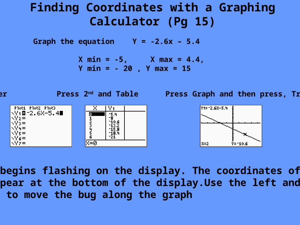
Finding Coordinates with a Graphing Calculator (Pg 15)

Press Y1 enter Press 2nd and Table Press Graph and then press, Trace and enter

“Bug” begins flashing on the display. The coordinates of the bug appear at the bottom of the display.Use the left and right arrows to move the bug along the graph

Graph the equation Y = -2.6x – 5.4

X min = -5, X max = 4.4, Y min = - 20 , Y max = 15

Using Graphing Calculator to solve the equation, (Pg 19)

Equation 572 – 23x = 181

Press Window and enter Press Y1 and Y2 and enter Press 2nd and Table

Press Graph and Trace

Y1 Y2

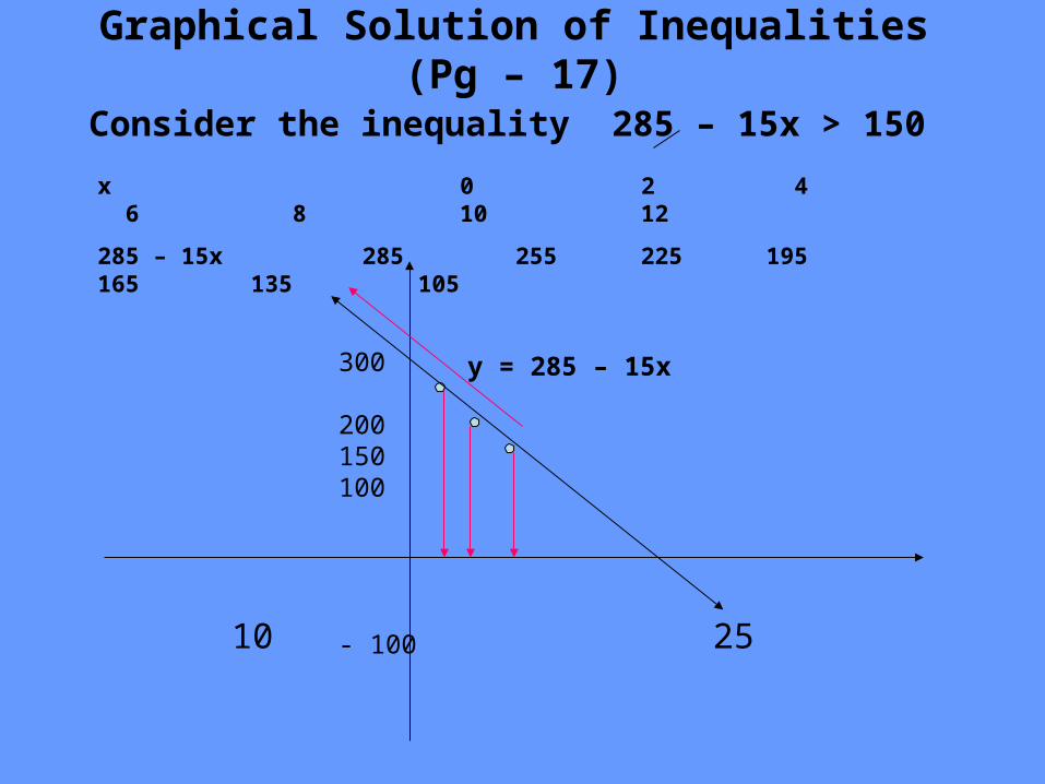
Graphical Solution of Inequalities (Pg – 17)

Consider the inequality 285 – 15x > 150

x 0 2 4 6 8 10 12

285 – 15x 285 255 225 195 165 135 105

10 25

300

200150100

- 100

y = 285 – 15x

1.3 Measuring Steepness ( pg 23)

Which path is more strenuous ?

5 ft

2 ft

Steepness measures how sharply the altitude increases..To compare the steepness of two inclined paths, we compute the ratio of changein horizontal distance for each path

1.3 Slope (Ex- 3, Pg 25)

Definition of Slope: The slope of a line is the ratio

Change in y- Coordinate

Change in x- coordinate

A B

0 2 3 4

54321

Slope = Change in y-coordinate = 5 - 4 = 1 Change in x- coordinate 4 – 2 2

Notation for Slope (Pg 26)

x

y

yxm = , where x is not equal to zero Slope of a line is given by

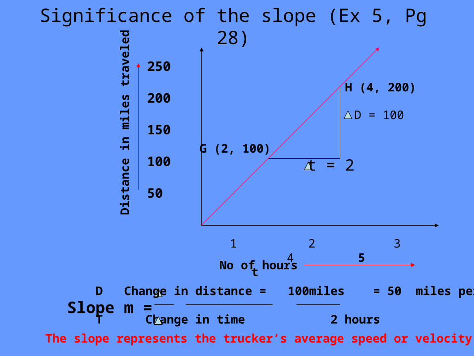
Significance of the slope (Ex 5, Pg 28)

1 2 3 4 5 t

250

200

150

100

50

t = 2

D = 100

H (4, 200)

G (2, 100)

D Change in distance = 100miles = 50 miles per hour

T Change in time 2 hoursSlope m =

No of hours

Dis

tan

ce i

n m

iles

tra

vele

d

The slope represents the trucker’s average speed or velocity

1.4 Equations of Lines ( Pg 40)

y = 2x

y = ½ x

y = -2x

These lines have the same y- intercept but different slopes

y = 2x + 3

y = 2x + 1

y = 2x - 2

These lines have the same slope but different y - intercepts

1.4 Slope – Intercept Formy = mx + b ( m is slope of a line, and b is the y- intercept)

3x + 4y = 6 Subtract 3x from both sides

4y = - 3x + 6 Divide both sides by 4

y = - 3x + 3

4 2

m= -3 and b = 3

4 2

General

Slope- Intercept Method of Graphing b Start here

New point

y = mx + b

x

y

A Formula for Slope

Slope Formula m = y2 – y1 = 9-(-6) -15 = - 3

x2 – x1 7 – 2 5

m = Y x

P1 (2, 9)

P2 (7, -6)

10

5

-5

10

The slope of the line passing through the points P1(x1, y1) and P2 ( x2, y2) is given by

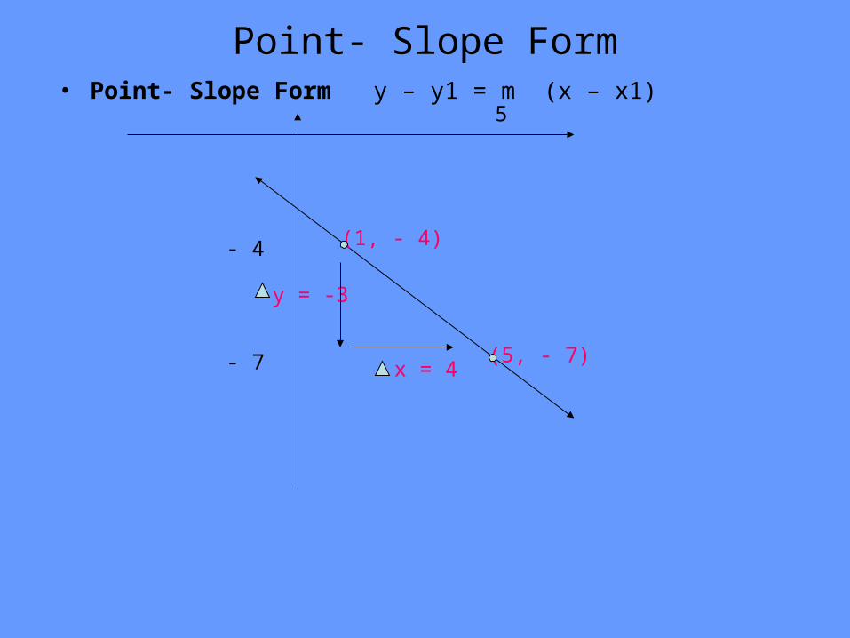
Point- Slope Form• Point- Slope Form y – y1 = m (x – x1)

x = 4

y = -3

(1, - 4)

(5, - 7)

5

- 7

- 4

ScatterPlots

scattered not organized decreasing trend increasing trend

1.5 Linear Regression (Lines of Best Fit)

The datas in the scatterplot are roughly linear, we can estimate the location of imaginary”lines best fit” that passes as close as possible to the data points

We can make the predictions about the data. The process of predicting a value

of y based on a straightline that fits the data is called a linear regression, and the line itself called the regression line.

The equation of the regression line is usually used(instead of graph) to predict values

Example of Linear Regression ( pg 55)

1000 2000Boiling Point 0 C

200

100

Hea

t of

Vap

oriz

atio

n (k

J)

(900, 100)

(1560, 170)

a) Slope = m= 170 – 100 = 0.106 1560 – 900The equation of regression line isy- y1 = m(x – x1)y – 100 = 0.106(x – 900) , y = 0.106x + 4.6

b) Regression equation for potassium bromide , x = 1435y = 0.106(1435) + 4.6

a) Estimate a line of best fit and find the equation of the regression lineb) Use the regression line to predict the heat of vaporization of potassium bromide, whose boiling temperature is 14350C

Choose two points in the regression line

112

96

80

64

48

20 40 60 80 100 Age (months)

The graph is not linear because her rate of growth is not constant; her growth slows down as she approaches her adult height. The short time of interval the graph is close to a line, and that line can be used to approximate the coordinates of points on the curve.

Hei

ght (

cm)

Interpolation- The process of estimating between known data points

Extrapolation- Making predictions beyond the range of known data

Ex 1.5 No 13, Pg 65

Loss in Mass (mg)

Vol. Of GasCubic cm

20 40 60 80 100

100

80

60

40

20

a) Student E made a mistake in the experiment since for a loss in mass of 88mg according to a line passing through the other points, volume should have been about 68cm3 instead of 76 cm3

b) The line of best fit passes through points (0,0) and (80, 60). The slope is m = 60/80 = 0.75 the equation of line is y = 0.75xc) Let y = 1000d) 1000= 0.75x , x = 1333 1/3 The mass of 1000cm3 of the gas is about 1333mge) The density of unknown gas is 1333mg = 1333mg = 1333mg = 1333 mg/liter 1000cm3 1000militers 1 literSince oxygen has a density of 1330mg/liter, oxygen is the most likely gas

Hydrogen 8mg/literNitrogen 1160 mg/literOxygen 1330 mg/literCarbon dioxide 1830 mg/liter

Using Graphing Calculator for Linear RegressionPg 59

Step 1 Press Stat , choose 1 press Enter

Step 3 Stat, right arrow go to 4And enter

Step 4Press Vars 5 ,Right,Right , Enter

Step 5 Press 2nd, Stat Plot and enter

Step 2 Enter Y = 1.95x – 7.86

Step 6 the graph ( Pg 60)

1.6 Additional Properties of Lines ( pg 68)

Horizontal Line

y = 4 Horizontal line4

X axis

Y axis

- 5 5

( - 1, 4) (2, 4)

y = k( const) Horizontal LineSlope = 0

Vertical Line

X axis

Y axis

- 5 5

5

-5

x = 3

(3, 1)

(3, 3)

x = k (const) Vertical line Slope is undefined

Perpendicular Lines

Two lines with slopes m1 and m2 are perpendicular if and only if m2 = - 1/m 1

5-5

-5

5

y = 2/3 x -2y = -3/2 x + 3 3

- 2

X axis

Y axis

m 1 = 2/3m2 = -3/2= - 1/ m1

m 1m2

Parallel Lines

-5 5

- 5

5 y = 2/3 x + 2

y = 2/3 x -2

Two lines with slopes m1 and m2 are parallel if and only if m1 = m 2

X axis

Y axis

Show that the triangle with vertices A(0, 8), B(6, 2) and C(-4, 4) is a right triangle

(-4, 4) (6, 2)

(0, 8)A

B

C

Slope of AB= m1 = 2 – 8 = - 6 = - 1 6 - 0 6Slope of AC =m2 = 4 – 8 = - 4 = 1 - 1 = -1 = 1 = m2

- 4 – 0 - 4 m1 -1

AB is Perpendicular to AC

X axis

Y axis

Example 33 Pg 77

• A) Sketch the triangle with vertices A(-6, -3) , B ( - 6, 3), and C(4, 5).

• B) Find the slope of the side AC.• C) Find the slope of the side of the altitude from point B to

side AC• D) Find an equation for the line that includes the altitude

from point B to side AC

A ( - 6, - 3)

C ( 4, 5)B ( - 6, 3 )

6

-6

-6 6B ) Slope of side AC = - 3 – 5 = - 8 = 4 - 6 – 4 - 10 5C) Slope of the altitude from Pt. B to side AC is perpendicular to AC and therefore – 5 4D) y – 3 = -5/4 ( x + 6) , y = 3/2 x + 15/2