introduction of dsp technology into the bioelectronics
TRANSCRIPT

Introduction of DSP technology into the
BioElectronics Laboratory Class
By: Richard Perng
Supervised by: Professor Steve Bums
Submitted to the Department of Electrical Engineering and Computer Science
in Partial Fulfillment of the Requirements for the Degrees of
Bachelor of Science in Electrical Engineering and Computer Science
and Master of Engineering in Electrical Engineering and Computer Science
at the Massachusetts Institute of Technology
May 1999
) Copyright 1998 Richard Pemg. All rights reserved.
The author hereby grants to M.I.T. permission to reproduce andDistribute publicly paper and electronic copies of this thesis MASSACHUSETTS INSTI E
and to grant others the right to do so.
L S
Author:Department of Electrical Engineering and Computer Science
May 1999
Certified by:Thesis Advisor
Accepted by~~Arthur C. Smith
Chairman, Department Committee on Graduate Theses
1

Introduction of DSP technology into the
BioElectronics Laboratory Class
By: Richard Pemg
Supervised by: Professor Steve Bums
Submitted to the Department of Electrical Engineering and Computer Science
in Partial Fulfillment of the Requirements for the Degrees of
Bachelor of Science in Electrical Engineering and Computer Science
and Master of Engineering in Electrical Engineering and Computer Science
ABSTRACT
The goal of the thesis project was to create a DSP component that system designers can use like
other analog components. Discussed here is the result of creating such a component. The main
aspect of the discussion focuses around a program that was created to help the designer use such
a component in his system design. The Windows-based program, DSP-Interface, creates an
abstraction barrier between the user and the internal workings of DSP chip. The DSP-Interface
uses ActiveX controls to create black boxes to help the user visualize the DSP system.
MATLAB is used for the program's math-intensive calculations and DSP algorithms. Lastly, the
program generates assembly code to be compiled and downloaded to the engine.
2

Table of Contents
ABSTRACT ......................- .. .. .------------------------------------................................. 2
Table of Contents.......................--.........................................................................................3
1 Introduction ..............-............ . .-------------------------................................................-------- 4
2 Background..................-......--..--... .-----------------------------------............................................... 62.1 D igital Design ......................................................-------------------------------------.-............................................... 6
2.1.1 D esign of D iscrete-Tim e Filters................................................................................- -... --------------........... 7
2.1.2 FIR Filter D esign ..........................................................................----.... ---------------................................. 9
2.2 Texas Instrum ent TM S320C 50 ................................................................................................................... 10
2.3 M icrosoft A ctiveX control.......................................................................................................................... 12
2.3.1 Active X history .........................-................ ---. ------------------------............................................... 12
2.3.2 D efinition of A ctiveX ........................................................................................................................... 13
2.3.3 Three Parts of the ActiveX control ......................................................................... .............. 14
2.4 M ATLAB API.........................................------... -... -----------------------.------------............................................... 15
3 Project DSP-I........------...-----------------------------------------------.......................................................163.1 ActiveX controls - Black Box........................................................--.-------.--............................................... 16
3.1.1 Input and Output Black Boxes..........................................................-............................................. 18
3.1.2 FIR Black Box...............................--- ............- .. . - --- --- -- --- --............................................... 19
3.2 ActiveX - DSP-I Interface ............................................................----.--.. . ----------------.................................. 19
3.3 D SP-Interface: M ain Program ..................................................................................................................... 24
3.4 M A TLAB -D SP-I Interface........................................................................................................................ 27
4 Results .................. .--...------------------------------------------------............................................... 294.1 Graphs Created by M A TLAB .................................................................................................................... 29
4.2 Assembly Files.............................-...-----------..---------------------------------------................................................-------
5 Conclusions............-.-.--....------------------------------------------------------...............................................315.1 Applications...............................- . -- . . . -----.----------------..-------............................................... 31
5.2 Im provem ents......................- .........----- .... . ---------------------------------------............................................... 32
5.1.1 M ain D SP-I.................. ..........------------------------------------------------..-----............................................... 32
5.1.2 M ATLAB function call.......................................-........- ... --------------------............................................... 34
5.1.3 Black Boxes................... .................. . .----------------.. - --- ----................................................ 34
6 Acknowledgements.......-........-......---...----------------------------...............................................36
7 Appendix...........--....--------------------------------------------------------------...............................................377.1 Sample output ASM file ..........................................--....- - - ... - - - ----..................................... 37
7.2 ActiveX control - D SP-I interface specifications......................................................................................... 39
7.3 CBaseD SPControl........................................------------- ..... . --- -----. --...............................................41
7 References ..........--.--.--..--------------------------------------------------------............................................... 46
3

1 Introduction
When designing a circuit board or machinery, the designer has certain tools to help him
finish his task. These tools may include computer aided design programs, books, and circuit
diagrams. He also has a collection of "components" in his inventory. These components include
oscillators, switched-capacitor filters, operational amplifiers, and power regulators. These
analog components are usually termed functional components because they do a specified task.
The manufacturers provide terminal specifications and examples of these components embedded
in working circuits. The designer is responsible for working within the specifications and
sometimes establishing his own parameters such as output voltage, cut-off frequencies for filters,
and oscillatory frequencies. All of these, components, books, and CAD programs, help the
designer solve problems.
An example of such a problem might be designing a differential instrumentation amplifier
intended to process an electrocardiogram (ECG) signal and present it to a recorder. This
instrument would require filtering for optimum signal-to-noise (SNR) performance. Most
designers would realize a filter using off-the-shelf components (such as the ones described
above). He would use CAD techniques to set the parameters of the filter such as the order of the
filter, the shape of the filter, and the pole-zero placement for the cut-off frequencies. CAD
programs would include FILT@, MATLAB@, National Instrumentation, and Simulink@. There
are reasons for this choice: cheap parts, analog signal, and familiar techniques for establishing
the specifications.
Now with cheaper and faster microprocessors, the designer can add DSP functional
components into his inventory. These DSP components would include a DSP "engine" which
acquires the signals, runs user-specified algorithms, and synthesizes the results. This engine
4

would include a library of algorithms and a set of tools. These tools would aid the designer to
select and load the algorithm into the engine, making it look like any other component in the
designer's inventory. The objective is to effectively use DSP technology in the same way analog
technology is used. With these tools, they serve to make the designer aware of the capabilities
and advantages of DSP technology without demanding that he know how to write the algorithms
or how to implement these algorithms on the engine.
An ideal situation would be as follows, taking the same example above with the differential
instrumentation amplifier. Say the designer wants a system that not only optimizes the SNR
performance but also wants linear phase filters. It is impossible to create a filter or series of
filters to have linear phase using analog components. This is commonly termed an unrealizable
analog filter. However using DSP components, this is conceivable. The designer will pick a
DSP component out of his inventory and use the component's tools to "program" the engine.
Then he will take this component and place it into his design as if the component was any of his
other analog components.
This paper talks about the implementation of such a DSP component. This DSP component
has a DSP engine, a library of algorithms, and a set of tools. The engine for this component is
the Texas Instrument (TI) DSK 320C50 starter kit. The algorithms are collected from selected
MATLAB@ functions that relate to digital signal processing. The set of tools includes the CAD
program DSP-Interface (DSP-I), compiler and linker. The DSP-I is a graphic window-based
program that helps the user program the engine. The compiler helps the user compile the code
generated by DSP-I to DSK format. The linker then downloads the DSK file into the engine and
starts the engine. Both the compiler and the linker come with the starter kit.
5

The paper is broken up as such: background, DSP-I, results, and conclusions. The
background talks about some of the necessary background information to understand the basis
behind. The DSP-I section explains the main project, the component that creates the barrier
between user and the underlying DSP engine. The results talks about the output files and graphs
generated by the DSP-I. Lastly, in the conclusions section, improvements are discussed.
2 Background
2.1 Digital Design
In the mid 1960s, digital signal processing started as a new branch of signal processing.
With the evolution of new and better digital processors, the idea of having real-time signal
processing became more feasible. Now, with faster and cheaper digital computers and
microprocessors, the idea of digital signal processing has become more of a feature than an
option. Fields such as data communications, sonar, radar, speech recognition, and biomedical
engineering have all benefited from DSP research and advancement. In the words of Oppenheim
and Schafer, "[t]he rapid evolution of digital computers and microprocessors together with some
important theoretical developments caused a major shift to digital technologies, giving rise to the
field of digital signal processing." (Oppenheim and Schafer, pg. 1)
s(t)
Continuous-Time Signal
s[n]
Sample of Continuous Signal
Figure 1 Sampling of CA signal to DT signal

"The fundamental aspect of digital signal processing is that it is based on processing of
sequences of samples." (Oppenheim and Schafer, pg.1-2) The most important part of these
sequencps of samples is the fact that they usually represent continuous-time (CT) signals. These
CT signals can be processed via digital technologies. In these cases, the continuous-time signals
are converted into discrete-time (DT) samples. After discrete-time processing, the samples are
converted back into CT signals. "Real-time operation is often desirable for such systems,
meaning that the discrete-time system is implemented so that samples of the output are computed
at the same rate at which the continuous-time signal is sampled." (Oppenheim and Schafer, pg.2)
The idea of using discrete-time filter and signal processing has come a long way for what it
was 20 to 40 years ago. Therefore, in order for the students to utilize as much of the
technological advances that DSP has to offer. The DSP-I will include all sorts of filters.
Therefore, the program must have implementation based on filter design issues. Furthermore,
there are two basic types of filters, infinite impulse response (IIR) and finite impulse response
(FIR).
2.1.1 Design of Discrete-Time Filters
The basic idea behind filters is the ability to modify certain frequencies relative to others.
The filter systems that use digital technology are commonly referred to as discrete-time filter.
When these DT filters are used for DT processing of CT signals, the specifications for both the
DT filters and CT filters are typically given in the frequency domain. Common frequency
domain filters include lowpass, bandpass, and highpass filters. Signals processed this way
usually proceed through three stages. First, the signal is sampled through an analog-to-digital
7

(A/D) converter. The signal then goes through the DT system. Finally, the processed signal is
converted back into a continuous-time signal through a digital-to-analog (D/A) converter.
In designing filters, they are usually calculated in continuous-time and then converted to
discrete-time because continuous-time filters design is more robust than discrete-time filters.
When converting filters from the continuous-time to the discrete-time case, there are two
methods of interest, impulse invariance and bilinear transform. "The concept behind impulse
invariance is the discrete-time system defined by sampling the impulse response of a continuous-
time filter" (Oppenheim and Schafer, pg. 407).
The other method is the bilinear transform. This is when the system function H(s) is changed
to the discrete-time equivalent H(z) or vise versa using the following equations:
S 2 (1 - 2-1)s= -4( (1)1d 1 + 2-1
Z 1 + (Td/ 2 )s (2)z = (2)
Equation 1 Bilinear Transform
This transformation wraps the imaginary axis of the s-plane around the unit circle of the z-
plane. (See figure below)
s-planeImage of
s=jQj (unit circle)
Image of
left half-plane
Figure 2 Bilinear mapping of s-plane and z-plane to each other
8

This transform avoids the problem of aliasing because it maps the entire imaginary axis of
the s-place onto the unit circle of the z-plane. However, this transformation has non-linear
frequency compression. The design of the discrete-time filters using this method must either
tolerate or compensate for this non-linearity. (Oppenheim and Schafer, pg. 417)
2.1.2 FIR Filter Design
The one type of discrete-time filters is the Finite Impulse Response (FIR) filter. The FIR
filter is finite in the time domain. This means that after a certain time n=No, the impulse
response of the filter is zero, i.e. h[n] = 0 for n > No. "FIR filters are almost entirely restricted to
discrete-time implementations [as opposed to the HR filters which are transforms based on
continuous time IIR filters]. Furthermore, most techniques for approximating the magnitude
response of an FIR system assumes linear phase constraint, thereby avoiding the problems of
spectrum factorization that complicates the direct design of IIR filters." (Oppenheim and
Schafer, pg. 444)
Different Window Types
STt% bmckma.. -k- + amm ng
0.8 e+(S a - rtl tt
n.60
~0.2
0~ - /02 0 05
Tim, / (Sam lesFiur 3 Comnyue idw
9

FIR filters can be created using different techniques such as windowing, remez, and
constrained least square. The windowing technique will be talked about here. There are eight
different types of windows: Bartlett, Blackman, Rectangular, Chebyshev, Hamming, Hanning,
Kaiser, and Triangular. The four common windows are shown in figure 3 below. By selecting
the right window, the FIR filter will have the desired mainlobe width and peak sidelobe
amplitude. For instance, the Bartlett window has a wider mainlobe but has smaller sidelobe
amplitude than the rectangular window.
For instance, when designing a lowpass filter, the designer picks the cut-off frequency and
the desired sidelobe peak. Using these two values, the designer can find out which window to
use for the desired sidelobe peak and the filter length for that window. Relative sidelobe peaks
are as follows: rectangular is -13 dB, Bartlett is -25dB, Hamming is -41dB, and Blackman is -
57 dB.
2.2 Texas Instrument TMS320C50
The project uses the TI TMS320C50 starter kit as its DSP component. The starter kit has a
TMS320C50 DSP chip for its engine. The DSP chip is an industry standard fixed-point DSP
with 50 ns instruction cycles. The starter kit has 10K on-chip RAM for storing user application
programs. There is also a 32K, 8-bit Programmable Read-Only Memory (PROM) for containing
the kernel program.
The DSK came with a window-based debugger for easy development and debugging. It also
comes with an assembler to assemble user written assembly code. The DSK communicates with
the PC through RS-232 serial port.
The kit also has a TLC32040 Analog Interface Circuit (AIC) for the kit's analog-to-digital
and digital-to-analog converter. The AIC is single-channel, input/output, and voice-quality
10
analog interface. It has a dynamic range of 14 bits. It also has variable D/A and A/D sampling
rate and filtering. The kit has two RCA jacks for receiving and transmitting analog signals. The
AIC is connected to the DSP chip through the 'C50 serial port. The 'C50 provides a maximal
10MIHz timer output to the master input clock of the AIC. The AIC is hard-wired for 16-bit
word mode operation and the reset pin of the AIC is connected to the BR pin of the 'C50.
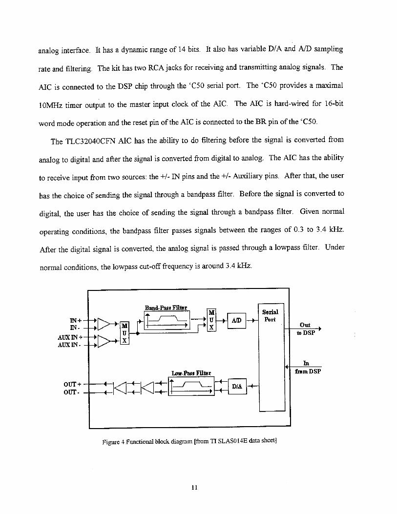
The TLC32040CFN AIC has the ability to do filtering before the signal is converted from
analog to digital and after the signal is converted from digital to analog. The AIC has the ability
to receive input from two sources: the +/- IN pins and the +/- Auxiliary pins. After that, the user
has the choice of sending the signal through a bandpass filter. Before the signal is converted to
digital, the user has the choice of sending the signal through a bandpass filter. Given normal
operating conditions, the bandpass filter passes signals between the ranges of 0.3 to 3.4 kHz.
After the digital signal is converted, the analog signal is passed through a lowpass filter. Under
normal conditions, the lowpass cut-off frequency is around 3.4 kHz.
Band-pass Filter -M Serial
IN+ - -+ -- +0 U -Po/ -- 1rtIN- - -- M T _XOu
A U X I N + - - + X
AUX IN - -
Low-Pass Filter frm DSP
OUT+ - ---- -- <-- - - DA +OUT - -+- -- 1
Figure 4 Functional block diagram [from TI SLASO14E data sheet]
11

The AIC sampling frequency works through six registers. They are divide three registers,
RA, RA', and RB, for the A/D conversion and three registers, TA, TA', and TB, for the D/A
conversion. The TA and RA are five bit registers with range from 4 to 31. The TA' and RA' are
six bit registers with range from 1 to 31. If TA or RA is ever lower than four, the AIC stops
working. If TA +/- TA' is lower than one, it will reset the AIC. TB and RB are six bit registers
with the range between 2 and 63. If TB or RB is zero or one, the registers are reprogrammed
with 24 hex.
The TA and TA' registers control the cut-off frequency for the lowpass filter. The RA and
RA' registers control the passband edges for the band-pass filter. Both filters are switch
capacitor filters. Therefore, the cut-off frequencies change depending on what clock frequency
is inputted into the filters.
For more information on the AIC used on the TMS320C50 starter kit, please refer to TI
SLASO14E data sheet. For more information on the starter kit, please refer to TMS320C5x DSP
Starter Kit: User's Guide.
2.3 Microsoft ActiveX control
2.3.1 Active X history
The DSP-Interface program uses ActiveX controls' for the "black boxes" found on the
editing area. The definition of ActiveX has gone through many changes since the name first
appeared. Before ActiveX and 32-bit Windows, Microsoft 16-bit Windows@ had Visual Basic
1 The definition of controls also has gone through a lot changes over the years. The definition that will be used in this paper is an
object/gizmo that can send and receive messages to its container. The container of the control can get/set properties and activates
methods.
12

Controls (VBX). These controls could export methods2 and exposed properties3 . These controls
were great for the 16-bit Windows system. However, the technique that made VBX controls
efficient in 16-bit Windows were heavily tied not only to the Intel chip, with lots of assembler
code, but also into the 16-bit segmented architecture, particularly the stack frame. When 32-bit
Windows came out, porting the VBX controls over would require a complete rewrite and lead to
other problems. Therefore, Microsoft decided to take the top-notch level concepts of the VBX
architecture and implement it using the new OLE4 2.0 specification, and they called their new
control mechanism OCX. In spring of 1996, the name was changed to ActiveX. (Platt, 144)
2.3.2 Definition of ActiveX
The definition of ActiveX control has gone through many changes. According to Platt:
"The term 'ActiveX' has gotten an enormous amount of airplay since its release in the spring of 1996. As
usual. once Microsoft finds an adjective they like, the tack it onto everything in sight until it loses all
meaning. as they did with the word 'Visual', leading to a great deal of confusion." (Platt, 145)
The term was originally defined:
-The term ActiveX originally referred to an extension of existing OLE and COM technologies, codenamed
"Sweeper", that allowed OLE-aware apps to do useful things with and over the Internet. A little later,
Microsoft declared that ActiveX controls was to be the new name of all OLE controls, whether or not they
had anything to do with the Internet Then ActiveX Components meant any in-proc COM or OLE server,
and then it meant all of COM except for object linking and embedding.... Then ActiveX Documents deal
2 Methods are functions that a container calls directly and passes an arbitrary number of parameters.
3 Properties are data values that the container could directly set or get
4 OLE stands for Object Linking and Embedding. Version 2.0 had better object linking and embedding functionality. Itcontained enhancements such as in-place activation and object linking that actually worked. It replaced the old Dynamic DataExchange (DDE) with Component Object Model (COM) as its underlying communication protocol. However, now a day, thedefmition of OLE is "just a collection of random syllables that Microsoft likes enough to trademark that refers to the entire set oftechnologies built on top of COM." (Platt, pg. 2)
13

with embedding and linking over the internet. But the term ActiveX isn't a replacement for the term
COM." (Platt, 145)
In this project, ActiveX controls mean the in-proc server with properties and methods, events
user interfaces and programming support, of the type created by the MFC.
2.3.3 Three Parts of the ActiveX control
When creating ActiveX controls in Microsoft Visual C++, each ActiveX control has three
main classes: a subclass of COleControl, a subclass of COleControlModule, and a subclass of
COlePropertyPage.
When inheriting from the COleControl class, the in-proc activation code and underlying
control technology is coded. Therefore, the user does not need to code these properties. The
class provides most of the nuts-and-bolts functionality common to all ActiveX controls. Two
important functions include event firing and dispatch map.
Get or set prperties.
Fire events. to the e
Figure 5 Interaction Between an ActiveX Control Container and aWindowed ActiveX Control
Event firing is similar to sending messages to control containers when certain conditions are
met. These events are used to notify the control container when something important happens in
the control. Additional information about an event can be sent to the control container by
attaching parameters to the event. (MSDN, ActiveX Controls)
The other important feature is the dispatch map, which is used to expose a set of functions
(called methods) and attributes (called properties) to the control user. Properties allow the
14

control container or the control user to manipulate the control in various ways. The user can
change the appearance of the control, change certain values of the control, or make requests of
the control, such as accessing a specific piece of data that the control maintains. This interface is
determined by the control developer. (MSDN, ActiveX control)
The COleControlModule class gives the ActiveX control the ability to act like a server. This
gives the subclass ActiveX control the ability to initialize the application (and each instance of it)
and to run the control as a server.
Lastly, the COlePropertyPage class lets the user of the ActiveX control to change properties
at run-time and at design-time. "These properties are accessed by invoking a control properties
dialog box, which contains one or more property pages that provides a customized, graphical
interface for viewing and editing the control properties." (MSDN, ActiveX Controls: Property
Pages.)
For more information concerning ActiveX controls, see MSDN Library Visual Studio 6.0.
2.4 MATLAB API
MATLAB is able to run as its own program or secondary to another program. In this project,
MATLAB is used for its math capabilities. The MATLAB engine can be accessed through the
dynamic link library (DLL) libeng.dll. The DLL has six main methods: engClose,
engEvalString, engGetArray, engOpen, engOutputBuffer, and engPutArray. The engOpen
method turns on the MATLAB engine. The engClose method turns off the MATLAB engine.
The engEvalString method is called to evaluate the MATLAB code. The engPutArray and
engGetArray place and grab matrices from MATLAB. Using the engOutputBuffer method, the
caller can grab output from MATLAB.
15

MATLAB also gives the ability to manipulate matrices after they are retrieved from the
engine. The dynamic link library libmx.dll has all the methods for manipulating matrices. In
this project, the libmx.dll is used to retrieve the data from matrices returned by the method
engGetArray. The libmx.dll has a myriad of methods for creating matrices and retrieving data
from matrices.
For more information on MATLAB, please go to the website http://www.mathworks.com.
3 Project DSP-I
The main aspect of the thesis is the development of the user interface. This interface
program, DSP-I, creates an abstraction barrier between the TI assembly code and DSP
algorithms. With this software, the designer who wants to add a DSP component into his design
need only insert the desired effects into the software and download the algorithm into the DSP
engine. He is not required to understand or even write engine specific assembly code to use the
DSP engine in his design.
This main section is broken down into mini-sections. The first section describes the black
boxes. The next section discusses the interface between the black boxes and the program. The
third section describes how the main DSP-I program works. Finally, the last section explains the
interface between the DSP-I and the MATLAB engine.
3.1 ActiveX controls - Black Box
In the DSP-I program, the user uses "black boxes" to create his system. These black boxes
can be created, destroyed, moved around, and linked to other boxes. These "Lego-style" black
boxes are constructed using ActiveX control technology. ActiveX controls can be dynamically
16

loaded at run-time and are also independent and self-contained. They have interfaces that link to
the outside world. These afore mentioned attributes are needed for a system that does not
provide prior knowledge to the containers.. Since the DSP-I program only specifies the
interface for the black boxes, the ActiveX control technology can be used to create these black
boxes.
Each black box is created separate from the others. Each box has its own way of handling
data, its own way of dealing with user-input, and its own way of managing event handles. Thus,
each box can be radically different from each other.
Microsoft Visual C++ ActiveX control builder was used to create the three black boxes in the
program: input box, output box, and FIR box. Originally, these boxes were designed to be a
subclass of a general template ActiveX control class which handled the basic features such as
drawing the control, resizing the control, and handling mouse events. However, an efficient way
Input
OutPut
Figure 6 how messages and calls are handled using the Template Control Class as the base classfor handling events.
17

to subclass the general ActiveX control was not found, so a template control class was created.
The figure above describes how the new template control class interacts with the ActiveX control
and the dialog window.
The Template Control Class is also used for storing data. Data used by the dialog box and
the ActiveX control are both stored here as information. After the user inputs his desired
information, the data are transferred to the subclassed Template Control Class. Other uses of the
subclassed Template Control Class are described in later sections.
For gathering user-input, the Dialog Window format was used instead of the Property Page
format in order to keep the black boxes self-contained. In this project, the black box handles the
display of the dialog window. For example, if the property page format is used, the main
program will obtain the property page and display the page.
3.1.1 Input and Output Black Boxes
The first two boxes created were the Input and Output Black Boxes. These boxes contain the
information necessary to setup the analog interface control (AIC) for gathering input and
synthesizing output. Each of these boxes contains two dialog boxes, a basic dialog window and
an advanced dialog window. The basic dialog window assumes that the user has no knowledge
of the inner working of the AIC, so it calculates the actual sampling frequencies from a
theoretical frequency. In the advanced mode, the user is given the control of actual registers
inside the AIC.
The Input Black Box contains other options found on the AIC. This box lets the user choose
to tell the AIC to use regular inputs or auxiliary inputs. The box also contains a gain selector for
selecting the amount of gain desired. Lastly, it gives the option to activate a 300 Hz to 3.4 kHz
bandpass filter on the AIC.
18

As for added features of the Output Black Box, it gives the user the ability to adjust the
lowpass filter found on the AIC. The lowpass filter is located between the D-to-A converter and
the output. The user selects the desired lowpass filter cut-off frequency, and the black box
computes the frequency that can be obtained with the settings. If the user is in advanced mode,
he can change the AIC register directly to find the most-suitable cut-off.
3.1.2 FIR Black Box
The FIR Black Box is the ActiveX control which contains the functionality for creating a
Finite Impulse Response (FIR) filter. This includes the ability to choose between different types
of FIR filter designs. The user may view filter he designed, in both the time and the frequency
domain. The FIR Black Box also lets the user change the MATLAB code before it is sent to the
MATLAB engine. Furthermore, it lets the user change the filter tap values.
The FIR Black Box uses the MATLAB engine for all math-related functions. When the user
needs to view the filter that he has designed, the FIR box again uses MATLAB to plot the
desired view. This includes frequency response plots and time-domain plots. When the user is
ready to save the filter, the box uses MATLAB to calculate the filter tap values. The only FIR
design choice the user can select is the FIR1. [See Conclusions - Improvements section for
more detail.]
3.2 ActiveX - DSP-I Interface
As stated in the background section, the ActiveX control has three ways of communicating
with its parent: events, methods, and properties. The black boxes also use these channels to
communicate with the DSP-Interface. Because the container calls and receives events, methods
and properties via explicit identification (id) values, each box's interface with the container has
19

to be created explicitly in order. Using the incorrect order can cause faulty interpretation of
events, wrong assessments of box properties, and incorrect calling of box methods.
All the black boxes possess these events: MouseDown, MouseMove, KeyDown, Evaluate,
GetMatrix, DoneWithMatrix, and GetSamplingFrequency. The first three events are stock
events5 . The Evaluate event fires when the black box needs to compute something using
MATLAB. The black box uses the GetMatrix event to signal to the DSP-I to retrieve a matrix
from MATLAB. The black box fires the DoneWithMatrix event to tell the DSP-Interface that it
is finished with the matrix. Finally, the black box fires the GetSamplingFrequency event to find
the sampling frequency value of the system.
The black boxes have a way of communicating to the DSP-I, so the DSP-I must also have a
way of communicating to the black boxes. The black boxes have 13 methods and 3 properties
through which the DSP-I can communicate. The properties are ImageSize, Animate, and
SamplingFrequency. The ImageSize property controls the size of the box. The Animate
property controls the animation sequence of the box. Lastly, the SamplingFrequency property
holds the value of the sampling frequency for the black box.
The black box's 13 methods help the DSP-I set and grab values. The DSP-Interface uses the
first two methods, SetMouseDown and SetMouseUp, to inform the black box that it has been
selected or unselected, respectively. If the black box is selected, it shows a different picture in
the window than when it is unselected.
Since black boxes are the building blocks of the system, they must convey to the container
which connections are valid. The DSP-I uses the methods GetInputType and GetOutputType to
make sure the connections are correct. These two methods return 0, 1, 2, and 3 depending what
20

the box can take (input) or give (output). If the method returns a zero, it means that an error
occurred while calling the method. A return value of one means the black box has no input for
GetlnputType and no output for GetOutputType. For GetInputType method, a value of two
means the black box receives time based values. A value of three corresponds to the black box
receiving frequency-based values. For GetOutputType, a value of two means that the black box
outputs values in time, and a value of three means that the black box outputs values in frequency.
Besides knowing what connections are valid, the black boxes must also convey to the
container where to draw these connections. The boxes support two methods, GetlnputLinePoint
and GetOutputLinePoint, to tell the container where to draw these connections. These two
methods return the coordinates in the form of strings. Each string is created in this order: x-
coordinate followed by a comma then the y-coordinate6 . The coordinate's origin is the top-left
corner of the black box.
DSP-Interface Black Box
Start MATLAB Evaluation
Create BSTR memoryblock for holding MATLABcode string
Process MATLAB code - - Fire Evaluation Event
l DDestroy BSTR memoryClDoneWithEvaluation block
Any more strings Yesto evaluate?
Figure 7 Flow Chart of how the black box talks to the DSP-I to calculate MATLAB code
5 Stock Events are events that Microsoft Visual C++ think that the programmer will most likely use, so they are preconstructedwith their own set of identification numbers and parameters. I.e. MouseDown has the id number of DISPIDMOUSEDOWN,and KeyDown has the id number of DISPID_KEYDOWN.6,"xy -ie "1,3"or"2_34,569"
21

Since the black boxes may need to know when MATLAB is done computing, the DSP-I must
relate this information to the black box. The three methods, PlaceMatrix, DestroyMatrix, and
DoneWithEvaluation, work with the events Evaluation, GetMatrix, and DoneWithMatrix to
communicate back and forth with the DSP-I to execute MATLAB calls. The picture above
shows how the black box and DSP-I use the Evaluation Event and the DoneWithEvalution
method to execute MATLAB code.
The following picture shows how the black box and the DSP-I communicate to retrieve
matrix values from MATLAB to the black box. The Matrix Object is a structure that holds the
DSP-Interface Black Box
Gather Data from MATLAB4,
Create BSTR memory blockfor string name of the matrix
4,Create Matrix Object 4 Fire GetMatrix Event
Get Matrix from MATLAB
Call PlaceMatrix -+ Get Data from Matnx
Destroy Matrix Object -- - Fire DoneWithMatrix Event
Call DestroyMatrix -- + Destroy BSTR memory block
More data to get from YesMATLAB?
Figure 8 Flow Chart of how MATLAB data is retrieved from the DSP-I.
matrix values found in MATLAB. These values must be of type double. If the value is not a
double or an array of doubles, the PlaceMatrix method will not work. The assumption in making
PlaceMatrix only transfer doubles is due to the fact that the filter tap are usually given as type
22

double. Therefore, the DSP-I does not need other methods to transfer other types of data to the
black box. In both, executing MATLAB code and retrieving data, the BSTR memory blocks are
created and destroyed to free resources.
Since all the data is stored on the black box, the DSP-Interface acquires this data to compile
the TI specific assembly code and download this code to the TI DSP chip. The four remaining
methods help the DSP-Interface obtain TI assembly code from the black box. The first of the
four methods is ReadyForDownload. This method returns true if the black box is ready for
compilation and downloads. The DSP-I uses this method to figure out if it is ready to call the
last three methods. If the method returns false, the DSP-I knows the black box is not ready for
download and the information returned from the last three methods may not be correct.
The last three methods, GetVariables, GetMemoryLayout, and GetExecutionCode, returns
the information needed for the DSP-I to place the black box's system into the overall system
assembly code. The GetVariables method returns a string of all the variables used in the
memory layout and the execution code. Each variable in the string is separated by a comma.
There are two variables not included in the GetVariables: <INPUT> and <OUTPUT>. These
two variables are assumed to be a part of every Execution code. If the black box has an output,
then it will have an <OUTPUT> variable in the execution code. If the black box has an input,
then it will have an <INPUT> variable in the execution code.
The GetMemoryLayout method returns a string containing the memory layout. It includes
constants and variables that are used in the execution code. In the FIR black box, the memory
layout includes the filter taps and the previous input values.
The GetExecutionCode method returns the string containing the assembly code for running
the engine. The DSP-I looks for six tags in the execution code: RECEIVEBEGIN,
23

RECEIVEEND, TRANSMIT_BEGIN, TRANSMIT_END, WAITBEGIN, and WAITEND.
These tags tell the DSP-I compiler where to place the assembly code. Some code must be run
immediately after the engine receives the receive interrupt. Other code requires the code be run
when the engine receives a transmit interrupt. Finally, codes that do not need execution after
interrupts are placed in the "wait" section of the code. The "wait" codes are executed when the
engine is waiting for either a transmit interrupt or a receive interrupt.
For a complete listing of the events, methods, and properties and their specifications, please
see the Appendix.
3.3 DSP-Interface: Main Program
The DSP-Interface is the main program that the user will interact with once he starts up the
program. The main program dynamically loads, holds, and displays the black boxes. It is in a
document/view form. The program threads a secondary thread for processing MATLAB code.
Furthermore, it handles all events coming from the secondary thread and black boxes. Lastly,
the program takes the different assembly codes from black boxes and compiles them for
download to the TI DSP chip.
The main program is in the Document/View architecture. The document stores all the data
while the view displays the data. This architecture is selected because it separates the display of
the data from the data. This makes it possible for future designs to change the look and feel of
the program without changing the underlying data structure and functions. For further
information on the document/view architecture, please refer to MSDN Library Visual Studio 6.0.
In order for the DSP-Interface to dynamically create the black boxes, the DSP-I interfaces
with all the black boxes through a base class. This base class is a wrapper around the ActiveX
control. The wrapper has all the events, methods, and properties described above. It converts
24
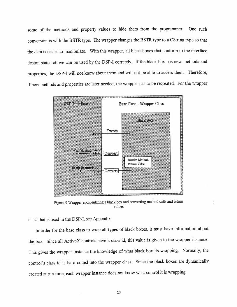
some of the methods and property values to hide them from the programmer. One such
conversion is with the BSTR type. The wrapper changes the BSTR type to a CString type so that
the data is easier to manipulate. With this wrapper, all black boxes that conform to the interface
design stated above can be used by the DSP-I correctly. If the black box has new methods and
properties, the DSP-I will not know about them and will not be able to access them. Therefore,
if new methods and properties are later needed, the wrapper has to be recreated. For the wrapper
Base Class -Wrapper Class
Events. . .............
....one . rt..M. o
Figure 9 Wrapper encapsulating a black box and converting method calls and returnvalues
class that is used in the DSP-I, see Appendix.
In order for the base class to wrap all types of black boxes, it must have information about
the box. Since all ActiveX controls have a class id, this value is given to the wrapper instance.
This gives the wrapper instance the knowledge of what black box its wrapping. Normally, the
control's class id is hard coded into the wrapper class. Since the black boxes are dynamically
created at run-time, each wrapper instance does not know what control it is wrapping.
25

Besides creating and maintaining the black boxes, the DSP-I also activates the MATLAB
engine and passes MATLAB related functions from the black boxes to the MATLAB engine. At
the start of the program, the MATLAB engine is closed, however the associated dynamically
linked libraries are accessed and opened. When requested, the engine opens and MATLAB runs
in the background. If the user needs, he can bring the window up to the front and access
MATLAB directly.
The MATLAB engine is opened on a secondary thread. The reason for having the MATLAB
engine resides on another thread is to allow the main program to continue while waiting for a
response from MATLAB. If anything goes wrong, the user can terminate the secondary thread
without affecting the main program. Furthermore, the user can continue to work while
MATLAB is computing.
Lastly, the DSP-I has the task of compiling the assembly code into a file. The program
checks the black boxes that are connected to either the Input Black Box or the Output Black Box
to see if they are ready for assembly. If any of the black boxes are not ready, the program
highlights the black box and cancels the compilation. If all the connecting boxes are ready, then
the program starts receiving data from the boxes.
The program goes through a series of checks and arrangements as it goes through the list of
boxes starting from the Input Black Box. With each box, the program checks the variables for
uniqueness. If there are similar variables found, the program changes the latest one by adding a
'x' to the end of the variable and changes the variable found in the memory layout and the
execution code.
With each black box, there is a possibility of an input and an output. If the compiler finds an
<INPUT> tag, it creates a variable INPUT*, where the * is the number of INPUT variables
26

found so far in the program. The compiler changes the tag in the execution code and places the
new variable in the memory layout. A similar task is performed on the <OUTPUT> tag. The
INPUT* and the OUTPUT* are the methods through which data is transferred between boxes in
assembly language.
In next step, the compiler deals with placing the execution code from each box in the rightful
place. There are three sections that the code can be placed: wait, receive, and transmit. The tags,
described in the previous section, are located, parsed, and placed into the correct section.
Finally, the compiler adds two pre-made files. The first file manages the initialization of the
DSP chip. The second file handles the initialization of the AIC.
3.4 MATLAB -DSP-I Interface
The interface between the DSP-I and MATLAB is performed through a threaded class
wrapper. The wrapper class hides the internal working of MATLAB functions from the main
program. This class supports the basic MATLAB API methods of opening the MATLAB
engine, closing the MATLAB engine, accessing output data, and obtaining matrices. The
wrapper class also has two other methods, CloseDLL and OpenDLL, for opening and closing the
MATLAB engine DLL, libeng.dll.
The DSP-I and the MATLAB wrapper communicate with each other through the posting of
messages. These messages go into a message queue. When a WMSTARTMATLAB-
COMPUTING tagged message is found in the MATLAB wrapper message queue, the wrapper
knows that the DSP-I wants the wrapper to start a MATLAB computation. Once the wrapper
receives this message, it creates an object that stores the necessary information, places it into a
MATLAB queue, and calls a queue service routine. The service routine is notified if there is
27

something in the queue. If there is something in the queue, the service routine will take the first
item, remove that item from the queue, and process the data stored in the first item.
Figure 10 Flow Chart of how MATLAB code is executed between the DSP-I and the MATLAB thread
28

Once the data has been passed into MATLAB, there are two possible results. One result
occurs when the user cancels the call, causing MATLAB to end prematurely. The MATLAB
wrapper sends a canceled message to DSP-I. The other result occurs when MATLAB finishes
executing the code. Then, the MATLAB wrapper to sends a message to the DSP-I stating that the
MATLAB code finished.
4 Results
4.1 Graphs Created by MATLAB
The FIR black box helps the user visualize the filter he has created by displaying the filter
through graphs. The FIR box calls MATLAB to display the theoretical filter and the actual
Frequency Plot with Rectangular W indow
1.5
0.5
00 1000 2000 3000 4000 6000 6000 7000 8000
50
0
-10
-1500 1000 2000 3000 4000 5000 6000 7000 8000
Frequency ( hz )
Figure 11 Plots displayed by the FIR Black Box through the MATLAB engine
29
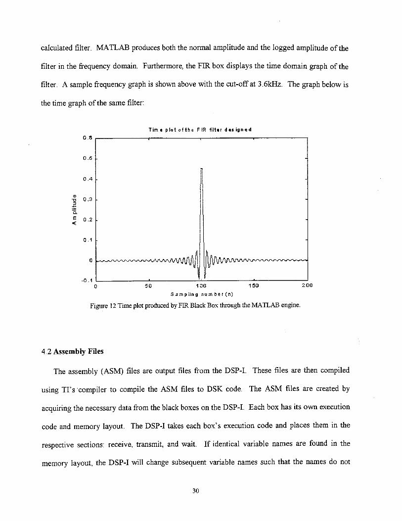
calculated filter. MATLAB produces both the normal amplitude and the logged amplitude of the
filter in the frequency domain. Furthermore, the FIR box displays the time domain graph of the
filter. A sample frequency graph is shown above with the cut-off at 3.6kHz. The graph below is
the time graph of the same filter:
Time plot of the FIR filter designed
0.6
0.4
0.3 -
E 0.2
0.1
-0.10 50 100 150 200
Sampling number(n)
Figure 12 Time plot produced by FIR Black Box through the MATLAB engine.
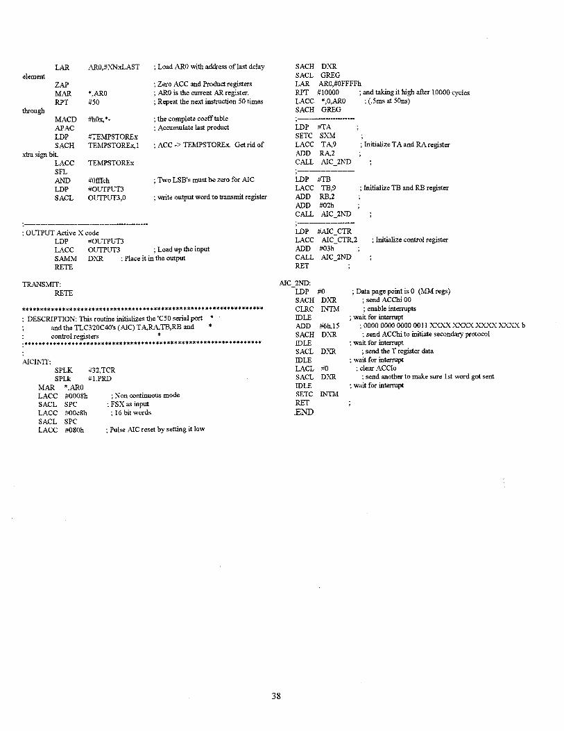
4.2 Assembly Files
The assembly (ASM) files are output files from the DSP-I. These files are then compiled
using TI's compiler to compile the ASM files to DSK code. The ASM files are created by
acquiring the necessary data from the black boxes on the DSP-I. Each box has its own execution
code and memory layout. The DSP-I takes each box's execution code and places them in the
respective sections: receive, transmit, and wait. If identical variable names are found in the
memory layout, the DSP-I will change subsequent variable names such that the names do not
30

interfere with each other. Besides assembly code found in the black boxes, the DSP-I inserts
assembly code for initializing the AIC given the variables found in the Input box and the Output
box. The program also places an interrupt initialization code for the DSP engine for interrupts
that deal with receiving data from the AIC and transmitting data to the AIC. Sample assembly
code can be found in the Appendix of this paper.
5 Conclusions
The DSP-Interface provides an abstraction barrier between the assembly code and the filter
design. The user needs only to know how he wants his filter to act, and the rest is done by the
interface program. The user can create different types of FIR filters using different window
designs and different cut-off frequencies. The user can change the sampling rate of the AIC on
the TI starter kit. Finally, the user has the ability to view his filter through graphs. Adding this
program to the TI compiler and TI linker completes the DSP component. The user has the
needed algorithms and the needed set of tools to help him set up the component to fit into the
system and act as any other component in his library.
5.1 Applications
There are many applications for the DSP-Interface. In schools, the professor can use the
program to help teach students digital signal processing through hands-on experience. The layer
of abstraction between the digital signal processing and TI specific assembly code helps the
professor give students the hands-on experience without the complications of teaching assembly
code. This lets the professor focus on teaching digital signal processing. Companies can use the
program to help simulate and test basic DSP systems and ideas before investing money into
creating the real system. DSP-I can also be used at home. Since programming the chip will be
31

easy, home-users and enthusiasts can place DSP engines throughout their system for different
purposes without programming in assembly.
DSP-I is a functional tool for the DSP component. The designer has the ability to use DSP
technology inside his designs without worrying about how to code the DSP engine. An example
is a student taking a laboratory class. The student is required to increase the SNR in his system.
Before, the student had only analog components at his disposal. With DSP-I, he is able to use
the TI starter kit as a component in his system. The student then generates the necessary ASM
code for operating the TI kit using the same program. He downloads the generated assembly file
and hooks up the TI Starter Kit to the rest of his system.
5.2 Improvements
As with all programs, there is never an end to the improvements and features one can add.
There will always be better ways of handling routines and designing dialog boxes. There will be
better ways of handling data storage and calculations. There will always be better ways of
writing help guides. The improvements given below are broken down into sections. Most of the
improvements address either the robustness7 of the program or key methods that were left out
due to time constraints.
5.1.1 Main DSP-I
One of the essential methods that were left out of the main DSP-I was the ability for the
program to call the TI compiler and TI linker. Currently the user must manually assemble the
code and download it onto the DSP chip. By adding this feature, the user can click on a menu
item and let the program handle the compilation and download. This feature was originally in
Robustness usually refers to the ability of the program to stay running if there is a human or computer generated eror. This
usually includes the wrong button push or wrong file access call.
32

the proposal. However, due to time constraint, this part of the program was never implemented.
The framework for including this feature is already in place. The remaining ideas and code to to
implement include determining how Microsoft VC++ handles DOS commands and how to
invoke executables from within the main program. By adding this feature, the program will truly
abstract the user from the TI assembly code and assembly calls.
The main program displays the MATLAB output in a window. Currently the program has
difficulties when accessing this window. Sometimes the program will crash when the window is
opened and then closed. Sometimes the program will crash with the window is opened, but the
error is not repeatable. Due to time constraint, the source of error was not found. Further
research should be conducted into correcting this error. For now, when using this program, be
careful when using the output window.
Another feature absent is the ability to dynamically add ActiveX controls to the program.
Currently, the ActiveX control class ID is hard-coded into the code. The user is unable to
dynamically add or subtract controls. Future versions will include the ability to dynamically
load user written ActiveX controls and dynamically change the different types of black boxes
available for the user at run-time.
Another feature missing is the ability to delete connections from one black box to another.
Currently the only way to delete connections is to delete the boxes that are connected. Some
attempts to implement this feature were made, but they all ended in failure. Future version will
make it possible to create connections and delete them without having to delete the boxes that are
connected.
Finally, the current program can only connect black boxes in series. The program is unable
to process connections in parallel. Adding this feature will be able to give the user more
33

flexibility in the way he creates the DSP component. This feature should be implemented after
the connection feature, as stated in the above paragraph.
5.1.2 MATLAB function call
The MATLAB engine currently is activated and called through threaded function calls.
Access to the MATLAB engine is relegated to a secondary thread. The reason behind this
design choice is that the MATLAB API does not seem to have a time-out response or cancel
function. Without either of these two features, the main program can call MATLAB and get
hung, locking out user input. However, during one of the many test runs, a dialog box appeared
from MATLAB stating that there in fact is a time-out in the MATLAB engine.
If MATLAB does have this time-out response mechanism, then it is possible for the
MATLAB engine to run on the main thread. By running MATLAB engine on the main thread, it
makes it possible to run this program with one less thread. Extra threads are taxing on the
system and memory. Furthermore, the program will not have to worry about faulty user input to
MATLAB because the MATLAB engine will return a time-out error.
5.1.3 Black Boxes
Because of time constraints, only the FIR black box was created, and it was created with
minimal functionality. Improvements would include finishing the FIR black box and adding
other boxes such as an Infinite Impulse Response (IIR) Black Box. These new boxes will help
the user create more sophisticated DSP components. Currently the interface between the
ActiveX control and the DSP-Interface is rigid and basic. Further research can redefine the
interface and make it more intuitive for future programmers to write their own black boxes.
34

The assembly code found in the black boxes was written hastily and not modular. Future
black boxes should have more efficient and more robust code.
Another improvement would be to give control of the bandpass cut-off frequencies to the
Input Black Box. Currently, the bandpass frequency is locked. By adding this new feature, the
user will have more control.
Finally, another improvement would be the ability to directly subclass from ActiveX
controls. Currently, the subclass is indirect. (See ActiveX controls - Black Box section for more
detail). If it is possible to directly subclass from an ActiveX control, then extra method calls8
can be saved, which in turn will create a more efficient system.
8 Method calls are expensive because they have overhead such as, stack pushes, stack pops, setting and cleaning local variables,and returning pointer.
35

6 Acknowledgements
I would like to thank my professor for helping through this thesis, from the proposal to
encouraging me while I programmed, and to the writing of the thesis. I would like to thank my
friends for not bugging me while I worked in my room. I would especially want to thank my
friend Shiu-Chung Au for proofreading my thesis and laughing at my grammar mistakes. I
would like to thank CBF for praying for me and making sure that I was doing okay. I want to
thank Janet Liu and Theresa Huang for being awake early in the morning to talk to me while I
wake up.
I want to that GOD for carrying me through the past two months of hard work. HE pulled
me through this tough endeavor.
36

7 Appendix
7.1 Sample output ASM file
DSPInterface Program Generated File!!!!!!;- -------- -------- --- .- - -- - - -
.MMREGS
.ds Of00hRA .word 18RB .word 20RAP .word 1AIC_CTR .word 8
SETC INTMLDP #0OPL #0834bPMSTLACC #0SAMM CWSRSAMM PDWSRSETC SXM SXM MUST BE SETSPLK #022hIMR ; This turns on receive interrupt only
OUTPUT1.word 0TEMPSTORE word 0
; FilterCoefficient Generator......hO .word 413,0,-448,1.491,0.,-542,1,607,0hi .word -686,1,793,0,-936,1,1145,0,-1472,1h2 .word 2061,0,-3434,1,10305,16186,10305,1,-3434,0h3 .word 2061,1,-1472,0,1145,1,-936,0.793.1h4 .word -686.0.607.1,-542,0.491.1,-448.0h5 .word 413
XNo
XN2XN3
.word 0,0,0,0,0,0,0.0,0,0
.word 0,0.0.0,0,0.0.0,0,0
.word 0.0.0.0.0,0,0.0.0.0
.word 0.0.0.0,0.0.0.0,0,0XN4 .word 0.0.0.0.0.0.0.0.0.0XNLAST .word 0
OUTPUT2.wordTEMPSTOREx
0.word 0
: FilterCoefficient Generator......hOx .word 413.0,-448.1.491.0,-542.1,607.0hl .word -686,1,793.0.-936.1.1145.0.-1472.1h2 .word 2061,0.-3434,1.10305,16186,10305,1,-3434,0h3 .word 2061.1.-1472.0,1145.1.-936.0,793,1h4 .word -686.0,607.1.-542,0.491,1,-448,0h5 .word 413
XNxo .wordXNx1 .wordXNx2 .wordXNx3 .wordXNx4 .wordXNxLAST.word
OUTPUT3.wordTA .wordTB .wordTAP .word
CALL AICINITSPLK #12hIMRCLRC OVMSPM 0CLRC INTM
WAIT:B WAIT
RECEIVE:--------- -------
INPUT Active X codeLAMM DRRLDP #OUTPUT1SACL OUTPUT1,0
FIR Active X code
CLRC INTMDEBUGGING DSK PURPOSES
LDP #OUTPUT1LACC OUTPUT1LDP #XNOSACL XN0LAR ARO,#XNLAST
elementZAP
through
0.0.0,0,0.0.0.0,0,00.0,0,0,0,0,0.0,0,00,0.0,0,0,0.0.0,0,00.0.0.0,0.0.0,0,0.00,0.0,0,0,0,0,0.0,0
18201
MAR *,ARORPT #50
MACD #hO,*-APACLDP #TEMPSTORESACH TEMPSTORE,1
xtra sign bit.LACC TEMPSTORESFLAND #0fffchLDP #OUTPUT2SACL OUTPUT2,0
;-------------- ---------FIR Active X code
CLRC INTMDEBUGGING DSK PURPOSES
LDP #OUTPUT2LACC OUTPUT2LDP #XNxOSACL XNx0
Start of Execution Code---------------------- --- ---- -- -- -- ------
.ps 0080ahrint: B RECEIVExint: B TRANSMIT
.ps OaOOh.entry
Load up the input
; Place it in for others to use
ENABLE INTERRUPTS FOR
Store OUTPUT1 value into a variableLoad ARO with address of last delay
Zero ACC and Product registers; ARO is the current AR register.; Repeat the next instruction 50 times
the complete coeff tableAccumulate last product
ACC -> TEMPSTORE. Get rid of
Two LSB's must be zero for AIC
write output word to transmit register
ENABLE INTERRUPTS FOR
Store OUTPUT2 value into a variable
37
element
through
LAR ARO,#XNxLAST
ZAPMARRPT
MACDAPACLDPSACH
xtra sign bit.LACCSFLANDLDPSACL
*,ARO#50
#hOx,*-
#TEMPSTORExTEMPSTOREx,1
TEMPSTOREx
#Offfch#OUTPUT3OUTPUT3,0
; Load ARO with address of last delay
; Zero ACC and Product registers; ARO is the current AR register.; Repeat the next instruction 50 times
; the complete coeff table; Accumulate last product
ACC -> TEMPSTOREx. Get rid of
Two LSBs must be zero for AIC
write output word to transmit register
SACH DXRSACL GREGLAR ARO,#OFFFFRPT #10000LACC *,0,AROSACH GREG;-----------------LDP #TASETC SXMLACC TA,9ADD RA,2CALL AIC_2ND
LDP #TBLACC TB,9ADD RB,2ADD #02hCALL AIC_2ND
and taking it high after 10000 cycles(.5ms at 50ns)
Initialize TA and RAregister
Initialize TB and RB register
OUTPUT Active X codeLDP #OUTPUT3LACC OUTPUT3SAMMRETE
; Load up the inputDXR ; Place it in the output
LDPLACCADDCALLRET
#AICCTRAICCTR,2
#03hAIC_2ND
; Initialize control register
TRANSMIT:RETE
DESCRIPTION: This routine initializes the 'C50 serial port *
and the TLC320C40's (AIC) TA,RA.TB,RB and *
; control registers *
AICINIT:SPLK #32,TCRSPLk #LPRD
MAR *,AROLACC #0008hSACL SPCLACC #00c8hSACL SPCLACC #080h
Non continuous modeFSX as input: 16 bit words
AIC_2ND:LDP #0SACH DXRCLRC INTMIDLEADD #6h,15SACH DXRIDLESACL DXRIDLELACL #0SACL DXRIDLESETC INTMRET.END
Data page point is 0 (MM regs)send ACChi 00enable interrupts
wait for interrupt0000 0000 0000 0011 XXXX XXXX XXXX XXXX bsend ACChi to initiate secondary protocol
wait for interrupt; send the T register data
wait for interruptclear ACClo; send another to make sure 1st word got sent
wait for interrupt
; Pulse AIC reset by setting it low
38

7.2 ActiveX control - DSP-I interface specifications
As stated in the main text, the interface between the ActiveX control and the DSP-I is rigid. The identificationnumbers have to be exact and the passing of arguments and results has to be exact. Below states the rules forcreating new ActiveX controls for use in the DSP-I.
Argument(s): Return type:
1 ImageSize float float
2 Animate boolean boolean3 SamplingFrequency double double
Methods:4 SetMouseDown void void5 SetMouseUp void void6 GetinputType void short
7 GetOutputType void short
8 GetinputLinePoint void BSTR9 GetOutputLinPoint void BSTR10 PlaceMatrix boolean, BSTR*, double* void11 DestroyMatrix BSTR* void
12 DoneWithEvaluation boolean void13 ReadyForDownload void boolean
14 GetVariables void BSTR15 GetMemoryLayout void BSTR
16 GetExecutionCode void BSTR
Events:DISPIDMOUSEDOWNDISPIDMOUSEMOVEDISPIDKEYDOWN1234
MouseDownMouseMoveKeyDownEvaluateGetMatrixDoneWithMatrixGetSamplingFrequency
short, snort, ULEA, ULEY
short, short, OLE_X, OLE_Yshort, shortBSTR*BSTR*BSTR*void
voidvoidvoidvoidvoidvoidvoid
The methods GetInputType and GetOutputType returns a short with the following number:0 errorI no connection2 time-based3 frequency-based
The methods GetinputLinePoint and GetOutputLinePoint returns a string in a specific order:
"<x-coordinate>,<y-coordinate>" if this is not followed correct, the DSP-I will not know where to paint the
connection lines.
The method GetVariables should return all the variables found in GetMemoryLayout. If not all the variables are
included here, there is a possibility that the compiler will miss identical variables. This might confuse the
assembler and the execution of the code after it is rnnning on the DSP chip
39
Type:Properties
Id: Name:

The method GetExecutionCode should have tags in it The tags used are RECEIVEBEGIN, RECEIVEEND,TRANSMITBEGIN, TRANSMITEND, WAITBEGIN, and WAITEND. These correspond to the different
sections that the TI assembly code can be placed: receive, transmit, and wait.
40

7.3 CBaseDSPControl
This class was used as wrapper for wrapping the black boxes found in the DSP-I
There is the header file and the CPP file:
41

// Machine generated IDispatch wrapper class(es) created by Microsoft Visual C++
/NOTE: Do not modify the contents of this file. If this class is regenerated by// Microsoft Visual C++, your modifications will be overwritten.
// CBaseDSPControl wrapper class
class CBaseDSPControl : public CWnd
{protected:
DECLAREDYNCREATE(CBaseDSPControl)public:
CLSID GetClsid() { return m clsid; }
void SetClsid(CLSID clsid) { m_clsid = clsid; }
virtual BOOL Create(LPCTSTR lpszClassName,LPCTSTR lpszWindowName, DWORD dwStyle,const RECT& rect,CWnd* pParentWnd, UINT nID,CCreateContext* pContext = NULL)
{ return CreateControl(GetClsidO, lpszWindowName, dwStyle, rect, pParentWnd, n]D); }
BOOL Create(LPCTSTR lpszWindowName, DWORD dwStyle,const RECT& rect, CWnd* pParentWnd, UINT nID,CFile* pPersist = NULL, BOOL bStorage = FALSE,BSTR bstrLicKey = NULL)
{ return CreateControl(GetClsido, lpszWindowName, dwStyle, rect, pParentWnd, nID,pPersist, bStorage, bstrLicKey); }
// Attributespublic:
float GetlmageSizeo;void SetImageSize(float);BOOL GetAnimateo)void SetAnimate(BOOL);double GetSamplingFrequencyo;void SetSamplingFrequency(double);
/Operationspublic:
void SetMouseDownO;void SetMouseUpo;short GetlnputTypeo;short GetOutputTypeo)CString GetInputLinePointo;CString GetOutputLinePointo;void PlaceMatrix(BOOL FoundIt, BSTR* variable, double* value);void DestroyMatrix(BSTR* variable);void DoneWithEvaluation(BOOL flag);BOOL ReadyForDownloadO;CString GetVariableso;CString GetMemoryLayouto;CString GetExecutionCodeo;void AboutBoxo;
private:CLSID m_clsid;
}
42

/ Machine generated IDispatch wrapper class(es) created by Microsoft Visual C++
/NOTE: Do not modify the contents of this file. If this class is regenerated by// Microsoft Visual C++, your modifications will be overwritten.
#include "stdafx.h"#include "templatedspcontroll.h"
// CBaseDSPControl
IMPLEMENTDYNCREATE(CBaseDSPControl, CWnd)
// CBaseDSPControl properties
float CBaseDSPControl::GetImageSize()
float result;GetProperty(Oxl, VTR4, (void*)&result);return result;
}
void CBaseDSPControl::SetmageSize(float propVal)
SetProperty(Ox1, VT_R4, propVal);
BOOL CBaseDSPControl::GetAnimate(){
BOOL result;GetProperty(0x2, VTBOOL, (void*)&result);return result;
}
void CBaseDSPControl::SetAnimate(BOOL propVal)
{SetProperty(Ox2, VT_BOOL, propVal);
}
double CBaseDSPControl::GetSamplingFrequency(){
double resultGetProperty(Ox3, VTR8, (void*)&result);return result
}
void CBaseDSPControl::SetSamplingFrequency(double propVal)
{SetProperty(0x3, VTR8, propVal);
// CBaseDSPControl operations
void CBaseDSPControl::SetMouseDown()
{InvokeHelper(0x4, DISPATCH_METHOD, VT_EMPTY, NULL, NULL);
void CBaseDSPControl::SetMouseUp(){
43

InvokeHelper(0x5, DISPATCH_METHOD, VT_EMPTY, NULL, NULL);}
short CBaseDSPControl::GetlnputType(){
short result;InvokeHelper(0x6, DISPATCH_METHOD, VTI2, (void*)&result, NULL);return result;
I
short CBaseDSPControl::GetOutputType(){
short result;InvokeHelper(0x7, DISPATCH_METHOD, VT_I2, (void*)&result, NULL);return result;
I
CString CBaseDSPControl::GetInputLinePoint()
CString result;InvokeHelper(0x8, DISPATCH_METHOD, VT_BSTR, (void*)&result, NULL);return result
}
CString CBaseDSPControl::GetOutputLinePoint(){
CString resultInvokeHelper(0x9, DISPATCH_METHOD, VTBSTR, (void*)&result, NULL);return result;
}
void CBaseDSPControl::PlaceMatrix(BOOL FoundIt, BSTR* variable, double* value){
static BYTE parns[]=VTS_BOOL VTS_PBSTR VTSPR8;
InvokeHelper(Oxa, DISPATCH_METHOD, VT_EMPTY, NULL, parms,FoundIt, variable, value);
}
void CBaseDSPControl::DestroyMatrix(BSTR* variable)
static BYTE parms[]=VTSPBSTR;
InvokeHelper(Oxb, DISPATCH_METHOD, VT_EMPTY, NULL, parms,variable);
}
void CBaseDSPControl::DoneWithEvaluation(BOOL flag)
static BYTE parms[]=VTSBOOL;
InvokeHelper(Oxc, DISPATCH_METHOD, VT_EMPTY, NULL, parms,flag);
}
BOOL CBaseDSPControl::ReadyForDownload(){
BOOL result;InvokeHelper(Oxd, DISPATCH_METHOD, VTBOOL, (void*)&result, NULL);return result;
I
44

CString CBaseDSPControl::GetVariables()
{CString result;InvokeHelper(Oxe, DISPATCH_METHOD, VTBSTR, (void*)&result, NULL);return result;
I
CString CBaseDSPControl::GetMemoryLayout(){
CString result;InvokeHelper(Oxf, DISPATCH_METHOD, VTBSTR, (void*)&result, NULL);return result;
}
CString CBaseDSPControl::GetExecutionCode(){
CString result;InvokeHelper(Ox10, DISPATCH_METHOD, VTBSTR, (void*)&result, NULL);return result
I
void CBaseDSPControl::AboutBox(){
InvokeHelper(Oxfffffdd8, DISPATCH_METHOD, VT_EMPTY, NULL, NULL);
I
45

7 References
1) Oppenheim, Alan V. and Schafer, Ronald W, Discrete-Time Signal Processing, Englewood Cliffs, New Jersey,
Prentice Hall, 1989, pg. 1-2, 403-490.
2) Bums, Steve, "An electrocardiogram Detector for the Boston Museum of Science", MIT 6.121 class notes,
Cambridge, MA, 1998.
3) Huhta, James C. and Webster, J. G. "60-Hz Interference in Electrocardiography", IEEE Transactions on
Biomedical Engineering vol. BME-20, no. 2, March 1973.
4) Lilly, L. S., Pathophysiology of Heart Disease, pg. 65-71.
5) Bums, Steve, "General Overview", handout for MIT 6.121 class on BioElectronics Laboratory class, February,
1998.
6) Platt, Daivd S., The Essence of COM with ActiveX: A programmer's workbook. 2 d edition, Upper Saddle
River. NJ, Prentice Hall PTR, 1998.
7) MSDN Visual Studio CD Helper
8) MATLAB webpage: http://www.matworks.com
9) MATLAB: External Interface Guide. The MathWorks, Inc. 1994.
10) MATLAB: Student Edition User's Guide. Version 5. The MathWorks, Inc. Prentice-Hall, Inc. Upper Saddle
River, NJ. 1997.
11) TI TMS320C5x User's Guide. Custom Printing Company. Owensville Missouri. 1996.
12) TI TMS320C5x DSP Starter Kit: User's
Company. Owensville Missouri. 1996.
Guide Microprocessor Development Systems, Custom Printing
13) Analog Interface Circuit Data Sheet number SLASO14E - May 1995. Texas Instruments Incorporated.
46