introduction robotics lecture - day 3 out of 7.ppt · scara geometry introduction robotics, lecture...

1/39

Introduction Robotics

Introduction Robotics, lecture 3 of 7

dr Dragan Kostić

WTB Dynamics and Control

September-October 2009

Introduction Robotics

2/39

• Recapitulation

• Forward kinematics

Outline


• Inverse kinematics problem

3/39

Recapitulation


Recapitulation

4/39

Robot manipulators

• Kinematic chain is series

of links and joints.SCARAgeometry


• Types of joints:

– rotary (revolute, θ)

– prismatic (translational, d).

geometry

schematic representations of robot joints

5/39

Common geometries of robot manipulators


6/39

Forward kinematics problem

• Determine position and orientation of the end-effector as

function of displacements in robot joints.


7/39

DH convention for homogenous transformations (1/2)

• An arbitrary homogeneous transformation is based on 6

independent variables: 3 for rotation + 3 for translation.

• DH convention reduces 6 to 4, by specific choice of

the coordinate frames.


the coordinate frames.

• In DH convention, each homogeneous transformation has the form:

8/39

DH convention for homogenous transformations (2/2)

• Position and orientation of coordinate frame i with respect to

frame i-1 is specified by homogenous transformation matrix:

qi

q0

qi+1

xn

z0

zn


ai

qi

qi

x0

xi-1

xi

zi

zi-1

y0 yn

zn

di

αi‘0’ ‘ ’n

where

9/39

Physical meaning of DH parameters• Link length ai is distance from zi-1 to

zi measured along xi.

• Link twist αi is angle between zi-1

and zi measured in plane normal

to x (right-hand rule). ai

qi

q0

qi+1

xx

zi

xn

y0 yn

z0

zn

αi‘0’ ‘ ’n


to xi (right-hand rule).

• Link offset di is distance from origin

of frame i-1 to the intersection xi

with zi-1, measured along zi-1.

• Joint angle θi is angle from xi-1 to xi

measured in plane normal to zi-1

(right-hand rule).

ai

qi

x0

xi-1

xi

zi-1di

10/39

DH convention to assign coordinate frames1. Assign zi to be the axis of actuation for joint i+1 (unless otherwise stated zn

coincides with zn-1).

2. Choose x0 and y0 so that the base frame is right-handed.

3. Iterative procedure for choosing oixiyizi depending on oi-1xi-1yi-1zi-1 (i=1, 2, …, n-1):

a) zi−1 and zi are not coplanar; there is an unique shortest line segment from zi−1 to

zi, perpendicular to both; this line segment defines xi and the point where the


zi, perpendicular to both; this line segment defines xi and the point where the

line intersects zi is the origin oi; choose yi to form a right-handed frame,

b) zi−1 is parallel to zi; there are infinitely many common normals; choose xi as

the normal passes through oi−1; choose oi as the point at which this normal

intersects zi; choose yi to form a right-handed frame,

c) zi−1 intersects zi; axis xi is chosen normal to the plane formed by zi and zi−1;

it’s positive direction is arbitrary; the most natural choice of oi is the

intersection of zi and zi−1, however, any point along the zi suffices;

choose yi to form a right-handed frame.

11/39

Forward Kinematics


Forward Kinematics

12/39

Forward kinematics (1/2)

• Homogenous transformation matrix relating the frame oixiyizi to

oi-1xi-1yi-1zi-1:


Ai specifies position and orientation of oixiyizi w.r.t. oi-1xi-1yi-1zi-1.

• Homogenous transformation matrix Tji expresses position and

orientation of ojxjyjzj with respect to oixiyizi:

jjiiij AAAAT 121 −++= K

13/39

• Forward kinematics of a serial manipulator with n joints can be

represented by homogenous transformation matrix Hn0 which

defines position and orientation of the end-effector’s (tip)

frame o x y z relative to the base coordinate frame o x y z :

Forward kinematics (2/2)


frame onxnynzn relative to the base coordinate frame o0x0y0z0:

=

⋅⋅==

×1

)()()(

),()()()(

13

00

0

11

00

0

qqq

qq

nn

n

nnnn

xRH

qAqATH K

[ ];00013 =×

0

[ ]Tnqq L1=q

14/39

Case-study: RRR robot manipulator

-q3

x

x2

x3

y1

y2

y3

d2a3

d3

z2

z3

elbow

Introduction Robotics, lecture 3 of 7 x0

q1

q2

x1

y0

y1

z0

α1

d1

a2

z1

z2

waist

shoulder

elbow

α1 - twist angle

ai - link lenghts

di - link offsets

qi - displacements

15/39

DH parameters of RRR robot manipulator


16/39

Forward kinematics of RRR robot manipulator (1/2)

• Coordinate frame o3x3y3z3 is related with the base frame o0x0y0z0 via

homogenous transformation matrix:

== 32103 (q)(q)A(q)AA(q)T


=

× 131

03

03

0

(q)x(q)R

whereT

qqq ][ 321=qT

zyx ][)(03 =qx

]000[31 =×0

17/39

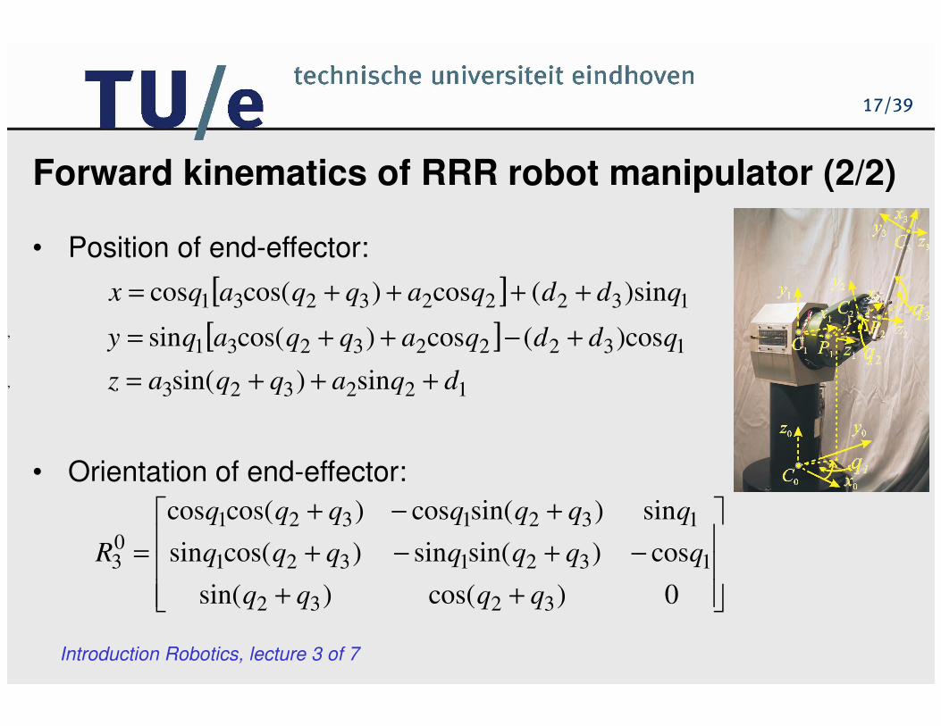
Forward kinematics of RRR robot manipulator (2/2)

,

• Position of end-effector:

[ ] 132223231 )sin(cos)cos(cos qddqaqqaqx ++++=

[ ] 132223231 )cos(cos)cos(sin qddqaqqaqy +−++=


, 122323 sin)sin( dqaqqaz +++=

• Orientation of end-effector:

++

−+−+

+−+

=

0)cos()sin(

cos)sin(sin)cos(sin

sin)sin(cos)cos(cos

3232

1321321

132132103

qqqq

qqqqqqq

qqqqqqq

R

18/39

Inverse Kinematics


Inverse Kinematics

19/39

Inverse kinematics problem

• Inverse kinematics (IK): determine displacements in robot joints that

correspond to given position and orientation of the end-effector.


20/39

Illustration: IK for planar RR manipulator (1/2)

• Elbow down IK solution


21/39

Illustration: IK for planar RR manipulator (2/2)

• Elbow up IK solution


22/39

The general IK problem (1/2)• Given a homogenous transformation matrix H∈SE(3)

find (multiple) solution(s) q1,…,qn to equation


find (multiple) solution(s) q1,…,qn to equation

• Here, H represents the desired position and orientation of the tip

coordinate frame onxnynzn relative to coordinate frame o0x0y0z0

of the base; T0n is product of homogenous transformation

matrices relating successive coordinate frames:

23/39

The general IK problem (2/2)

• Since the bottom rows of both T0n and H are equal to [0 0 0 1],

equation


gives rise to 4 trivial equations and 12 equations in n unknowns

q1,…,qn:

Here, Tij and Hij are nontrivial elements of T0n and H.

24/39

Illustration: Stanford manipulator


25/39

FK of Stanford manipulator


26/39

Example of IK solution for Stanford manipulator• Rotational equations (correspond to R0

6):


• Positional equations (correspond to o06):• One solution:

27/39

Nature of IK solutions• FK problem has always unique solution whereas IK problem may

or may not have a solution; if IK solution exists, it may or may not

be unique; solving IK equations, in general, is much too difficult.

• It is preferable to find IK solutions in closed-form:


– faster computation (e.g. at sampling time of 1 [ms]),

– if multiple IK solutions exist, then closed-form allows us to develop

rules for choosing a particular solution among several.

• Existence of IK solutions depends on mathematical as well as

engineering considerations.

• We assume that the given position and orientation is such that at

least one IK solution exists.

28/39

Kinematic decoupling (1/3)

• General IK problem is difficult BUT for manipulators having 6 joints

with the last 3 joint axes intersecting at one point, it is possible to

decouple the general IK problem into two simpler problems:

inverse position kinematics and inverse orientation kinematics.


inverse position kinematics and inverse orientation kinematics.

• IK problem: for given R and o solve 9 rotational and 3 positional

equations:

29/39


• Spherical wrist as paradigm.


• Let oc be the intersection of the last 3 joint axes; as z3, z4, and z5

intersect at oc, the origins o4 and o5 will always be at oc;

the motion of joints 4, 5 and 6 will not change the position of oc;

only motions of joints 1, 2 and 3 can influence position of oc.

30/39



⇒ q1, q2, q3

⇒

⇒ q4, q5, q6

31/39

Articulated manipulator: inverse position problem


• Inverse tangent function Atan2(xc,yc) is defined for all (xc,yc)≠(0,0)

and equals the unique angle θ1 such that:

,cos22

1

cc

c

yx

x

+=θ .sin

221

cc

c

yx

y

+=θ

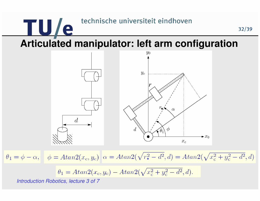
32/39

Articulated manipulator: left arm configuration

r


*

*

33/39

Articulated manipulator: right arm configuration

Introduction Robotics, lecture 3 of 7 +π*

*

r

34/39

*

r

Articulated manipulator: IK solution for θθθθ3


• Law of cosines:

+ elbow down; - elbow up

35/39

Articulated manipulator: IK solution for θθθθ2

υυυυ θ =υ - υ


υυυυ1

υυυυ2 θ2=υ1- υ2

υ1=Atan2(r,s)

υ2=Atan2(a2+a3cosθ3,a3sinθ3)

36/39

Four IK solutions θθθθ1-θθθθ3 for articulated manipulator

• PUMA robot as

an example of

the articulated

geometry.


geometry.

37/39

Articulated manipulator: inverse orientation problem

Introduction Robotics, lecture 3 of 7 • Equation to solve:

38/39

Articulated manipulator: IK solutions for θθθθ4 and θθθθ5

• Equations given by the third column in :


• If not both right-hand sides of the first two equations are zero:

±

• If positive square root is chosen in solution for θ5:

39/39

Articulated manipulator: IK solutions for θθθθ6

• The first two equations given by the last row in :

-s5c6 = s1r11 - c1r21

s5s6 = s1r12 - c1r22


• Analogous approach if negative square root is chosen in

solution for θ5.

• From these equations it follows:

introduction robotics lecture - day 3 out of 7.ppt · scara geometry introduction robotics, lecture...

Documents