introduction - 北海道大学eprints3.math.sci.hokudai.ac.jp/2409/1/pre1101.pdf · in summary, we...

AN ENERGETIC VARIATIONAL APPROACH FOR NONLINEAR

DIFFUSION EQUATIONS IN MOVING THIN DOMAINS

TATSU-HIKO MIURA, YOSHIKAZU GIGA, AND CHUN LIU

Abstract. This paper concerns the processes of nonlinear diffusion in a mov-ing domain which lies on a moving closed surface. The nonlinear diffusion

equations and corresponding energy identities are derived by regarding the

moving surface as a thin width (thickness) limit of moving thin domains, forwhich suitable boundary conditions are imposed to insure that there is no

exchange of mass between the thin domains and the environments. We also

employ an energetic variational approach to derive these nonlinear diffusionequations. Most of all, we show that these nonlinear energetic variational

procedures can commute with the passing to the zero width limits.

1. Introduction

In this paper, we are interested in deriving diffusion equations on a movingsurface, by regarding it as a limit of the problem in a moving thin domain with itswidth tends to zero.

Let us begin with an equation of the conservation of mass ρ with velocity u in amoving domain Ω(t) in Rn of the form

∂tρ+ div(ρu) = 0,(1.1)

which represents the local conservation of mass. Considering the situation thatthere is no exchange of mass on the boundary, i.e.

u · νΩ = V NΩ(1.2)

on the boundary, where V NΩ is the normal velocity of the boundary of the moving

domain Ω(t) in the direction of the outward normal vector field νΩ of the boundary.Similar conservation law of mass η with velocity v on a moving surface Γ(t) canbe derived from the local conservation of mass. It turns out (see Section 3) that,when the normal component of v is equal to the outward normal velocity V N

Γ ofthe moving surface Γ(t), the resulting equation is of the form:

∂η − V NΓ Hη + divΓ(ηvT ) = 0,(1.3)

where ∂ = ∂t + V NΓ νΓ is the normal time derivative, νΓ is the outward normal

vector field of Γ(t), H is the (n − 1 times) mean curvature of Γ(t), divΓ is thesurface divergence operator on Γ(t), and vT is a tangential vector field satisfyingv = V N

Γ νΓ + vT . Note that this equation is obtained as the zero width limit of thecorresponding equation (1.1) in a moving thin domain Ωε(t) defined as the set ofall points in Rn with distance less than ε from Γ(t) (see Remark 4.2).

The conventional diffusion equations, or even the porous-media equations, canbe viewed as the combination of incompressible fluids with the damping in the formof Darcy’s law. Take the usual Darcy’s law for the velocity u:

−ρu = ∇p(ρ)(1.4)

2010 Mathematics Subject Classification. 35B25, 35K55, 76R50.Key words and phrases. Nonlinear diffusion equation, Zero thickness limit, Moving surface,

Energetic variational approaches.

1

2 T.-H. MIURA, Y. GIGA, AND C. LIU

in the moving thin domain Ωε(t), where p is the pressure, then we can prove (seeTheorem 4.1) that the zero width limit of the diffusion equations (1.1) with (1.4)yields diffusion equations on the moving surface Γ(t): (1.3) and Darcy’s law

−ηvT = ∇Γp(η).(1.5)

Here vT is the tangential component of the velocity v and ∇Γ is the tangentialgradient on Γ(t).

The diffusion equations (1.1), (1.4) and (1.3), (1.5) possess specific energy iden-tities. It can be easily proven (see Section 5) that for ρ and u satisfying (1.1) and(1.4) the energy identity

d

dt

∫Ω(t)

ω(ρ) dx = −∫

Ω(t)

ρ|u|2 dx−∫∂Ω(t)

p(ρ)V NΩ dHn−1(1.6)

holds. Here ω is a function satisfying p(ρ) = ω′(ρ)ρ− ω(ρ). Similarly, for η and vsatisfying (1.3) and (1.5) we have

d

dt

∫Γ(t)

ω(η) dHn−1 = −∫

Γ(t)

η|vT |2 dHn−1 +

∫Γ(t)

p(η)V NΓ H dHn−1,(1.7)

where Hn−1 is the (n− 1)-dimensional Hausdorff measure. Fortunately, the energyidentity (1.7) on the moving surface can be derived as the zero width limit of theenergy identity (1.6) in the moving thin domain (see Theorem 5.3).

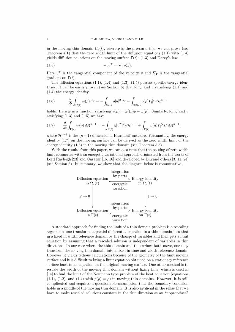
With the results from this paper, we can also note that the passing of zero widthlimit commutes with an energetic variational approach originated from the works ofLord Rayleigh [23] and Onsager [15, 16] and developed by Liu and others [3, 11, 24](see Section 6). In summary, we show that the diagram below is commutative.

Diffusion equationin Ωε(t)

integrationby parts //

ε→ 0

Energy identityin Ωε(t)energetic

variation

oo

ε→ 0

Diffusion equation

in Γ(t)

integrationby parts // Energy identity

on Γ(t)energeticvariation

oo

A standard approach for finding the limit of a thin domain problem is a rescalingargument: one transforms a partial differential equation in a thin domain into thatin a fixed in width reference domain by the change of variables and then gets a limitequation by assuming that a rescaled solution is independent of variables in thindirections. In our case where the thin domain and the surface both move, one maytransform the moving thin domain into a fixed in time and width reference domain.However, it yields tedious calculations because of the geometry of the limit movingsurface and it is difficult to bring a limit equation obtained on a stationary referencesurface back to an equation on the original moving surface. One other method is torescale the width of the moving thin domain without fixing time, which is used in[14] to find the limit of the Neumann type problem of the heat equation (equations(1.1), (1.2), and (1.4) with p(ρ) = ρ) in moving thin domains. However, it is stillcomplicated and requires a questionable assumption that the boundary conditionholds in a middle of the moving thin domain. It is also artificial in the sense that wehave to make rescaled solutions constant in the thin direction at an “appropriate”

ENERGETIC VARIATION FOR NONLINEAR DIFFUSION IN MOVING THIN DOMAINS 3

point to derive the limit energy identity and if we take a wrong point then we geta wrong limit (see Remarks 5.5).

To derive a limit with more straightforward calculations, we use another methodwhich comes from an idea for determining coefficients of polynomials of formalexpansion with respect to the width parameter ε: if A0, A1, . . . , An are independentof ε and

A0 + εA1 + · · ·+ εnAn +O(εn+1) = 0

for all ε > 0, then A0 = A1 = · · · = An = 0. We follow this idea but do not rescalethe width of the moving thin domain. Since the moving surface Γ(t) admits thenormal coordinate system

x = π(x, t) + d(x, t)νΓ(π(x, t), t)

for x ∈ Ωε(t), where π(x, t) is the projection onto Γ(t) and d(x, t) is the signeddistance function from Γ(t) increasing in the direction of the normal vector fieldνΓ, we expand the density ρ and the velocity u defined on Ωε(t) in powers of thesigned distance:

ρ(x, t) = η(π(x, t), t) + d(x, t)η1(π(x, t), t) + · · · ,u(x, t) = v(π(x, t), t) + d(x, t)v1(π(x, t), t) + · · · .

We differentiate both sides of the above equations and substitute them for equa-tions (1.1), (1.2), and (1.4). Then under suitable assumptions we obtain the limitequations (1.3) and (1.5) as the zeroth order terms of expansions in the signeddistance (or ε) of the original equations (1.1), (1.2), and (1.4) (see Section 4). Thesame idea is valid for derivation of the energy identity (1.7) on the moving surfacefrom that in the moving thin domain (1.6) (see Section 5). To get the limit energyidentity we also use integral transformation formulas from surface integrals overthe level-set surfaces x ∈ Rn | d(x, t) = r (−ε < r < ε) into that over the zerolevel-set surface Γ(t) (see Lemma 5.4).

There is a long history in the study of partial differential equations in thindomains, such as the pioneering work by Hale and Raugel [7, 8], where they in-vestigated damped hyperbolic equations and reaction-diffusion equations in a flatstationary thin domain of the form

Ωε = (x′, xn) ∈ Rn | x′ ∈ ω, 0 < xn < εg(x′),(1.8)

where ω is an open set in Rn−1 and g is a function on ω. There is also a large numberof the literature on reaction-diffusion equations in various types of thin domainssuch as a thin L-shaped domain [9], a moving flat thin domain of the form (1.8)with g time-dependent [17], and flat and curved thin domains with holes [18, 19, 20](here a curved thin domain is a thin domain degenerating into a lower dimensionalmanifold). A main subject in the above literature is to compare the dynamicsof equations in thin domains with that of limit equations in their degenerate setsrather than to find the limit equations of the original equations in the thin domains,since their degenerate sets are stationary and thus the rescaling argument workswell for finding the limit equations. The Navier–Stokes equations in thin domainshas been also studied well [10, 12, 22, 25, 26] since fluid flows in thin domains oftenappear in natural sciences like the flow of water in a large lake, geophysical flows,etc. Researchers are especially interested in the relation between the smallness ofthe width of thin domains and the large time behavior of solutions to the Navier–Stokes equations in thin domains. We refer to [21] and therein for other types ofthin domains degenerating into stationary sets and mathematical analysis of partialdifferential equations in such thin domains.


In the case where the degenerate set of a thin domain moves, derivation of thelimit of a partial differential equation in the thin domain is more complicated sincethe geometry of the degenerate set changes as it moves. Such a problem was firstconsidered in [14] where the author derived both formally and rigorously the limitequation of the Neumann type problem of the heat equation (equations (1.1), (1.2),and (1.4) with p(ρ) = ρ) in a moving thin domain degenerating into a closed smoothmoving surface. He also found that the normal velocity and the mean curvature ofthe degenerate moving surface affects the limit equation, which is not observed inthe case where the degenerate set of a thin domain does not move.

The rest of this paper is organized as follows. In Section 2, we fix some nota-tions on various quantities related to the moving surface. In Section 3, we brieflyobserve that the transport equations in the moving domain and the moving surfaceare equivalent to the local mass conservation. In Section 4, we derive the limitequations (1.3) and (1.5) on the moving surface from the diffusion equations (1.1),(1.2), and (1.4) on the moving thin domain by means of expansion in terms of thesigned distance. In Section 5, we derive the energy identities (1.6) and (1.7) fromcorresponding diffusion equations and then show that the energy identity (1.7) onthe moving surface is the zero width limit of the energy identity (1.6) on the movingthin domain. In Section 6, we apply an energetic variational approach to the energyidentities (1.6) and (1.7) to obtain Darcy’s laws (1.4) and (1.5).

2. Quantities on a moving surface

We start with several notations for a moving surface. Let Γ(t), t ∈ [0, T ] be aclosed (that is, compact and without boundary), connected, oriented and smoothmoving surface in Rn with n ≥ 2. We write νΓ(·, t) and V N

Γ (·, t) for the unit outwardnormal vector field and the scalar outward normal velocity of Γ(t), respectively (notethat to describe the evolution of a closed surface it is sufficient to give the normalvelocity). Since the smooth closed surface Γ(t) varies smoothly in time, the principalcurvatures κ1(·, t), . . . , κn−1(·, t) of Γ(t) are bounded uniformly in t ∈ [0, T ]. Thenthere exists a constant δ > 0 independent of t such that the tubular neighborhood

N(t) := x ∈ Rn | dist(x,Γ(t)) < δ

of Γ(t) admits the normal coordinate system

x = π(x, t) + d(x, t)νΓ(π(x, t), t)(2.1)

for each x ∈ N(t), where π(·, t) is the orthogonal projection onto Γ(t) and d(·, t) isthe signed distance function from Γ(t) (see [5, Section 14.6] for example). Here wesuppose that d(·, t) increases along the direction of νΓ(·, t). Then we have

∇d(x, t) = νΓ(π(x, t), t), x ∈ N(t),(2.2)

∂td(y, t) = −V NΓ (y, t), y ∈ Γ(t).

Moreover, differentiating both sides of

d(x, t) = x− π(x, t)∇d(x, t), d(π(x, t), t) = 0

with respect to t we easily obtain

∂td(x, t) = ∂td(π(x, t), t) = −V NΓ (π(x, t), t), x ∈ N(t).(2.3)

We write PΓ := In − νΓ ⊗ νΓ for the orthogonal projection onto the tangent spaceof Γ(t). Here In denotes the identity matrix of size n and a ⊗ b = (aibj)i,j is thetensor product of two vectors a = (a1, . . . , an) and b = (b1, . . . , bn) in Rn. We define


the tangential gradient of a function f on Γ(t) and the surface divergence of a (notnecessarily tangential) vector field F on Γ(t) as

∇Γf := PΓ∇f , divΓF := tr[PΓ∇F ].

Here f and F are the constant extension of f and F in the normal direction ofΓ(t) given by f(x) := f(π(x, t)) and F (x) := F (π(x, t)) for x ∈ N(t). Also, tr[M ]denotes the trace of a square matrix M and we use the notation

∇G =

∂1G1 . . . ∂1Gn

.... . .

...∂nG1 . . . ∂nGn

for the gradient matrix of a vector field G = (G1, . . . , Gn). Note that ∇Γf · νΓ = 0for any function f on Γ(t). We also define the (n− 1 times) mean curvature H ofΓ(t) as

H(y, t) := −divΓνΓ(y, t)(2.4)

for y ∈ Γ(t), t ∈ [0, T ]. Note that the mean curvature defined as above is equal tothe sum of the principal curvatures:

H(y, t) =

n−1∑i=1

κi(y, t), y ∈ Γ(t).(2.5)

Finally, we write ∂ = ∂t + V NΓ νΓ · ∇ for the normal time derivative (the time

derivative along the normal velocity). Note that the formula

∂f(y, t) =d

dt

(f(π(y, t), t)

), y ∈ Γ(t)(2.6)

holds for a function f(·, t) on Γ(t) (see [2, Section 3.4]).

3. Transport equation in a moving domain and on a moving surface

In this section we give the transport equation for a scalar quantity in a movingdomain and on a moving surface. We use some of the same terminology and tech-niques as in [13]. We first consider transportation of a scalar quantity in a boundedmoving domain Ω(t) in Rn. Let ρ(x, t) and u(x, t) be the density and the velocityfield of the scalar quantity at x ∈ Ω(t), respectively. Our starting point is the localmass conservation

d

dt

∫U(t)

ρ dx = 0(3.1)

for any portion U(t) (relatively open set) of Ω(t) moving with velocity u(·, t). Sincethe left-hand side is equal to

∫U(t)∂tρ+div(ρu) dx by the Reynolds transport the-

orem [6] and the divergence theorem, the condition (3.1) for any U(t) is equivalentto the transport equation

∂tρ+ div(ρu) = 0 in Ω(t), t ∈ (0, T ).(3.2)

To make the total mass∫

Ω(t)ρ dx conserved, we impose the boundary condition

u · νΩ = V NΩ on ∂Ω(t), t ∈ (0, T ),(3.3)

where νΩ(·, t) and V NΩ (·, t) are the unit outward normal vector field and the scalar

outward normal velocity of ∂Ω(t), respectively. The boundary condition (3.3) phys-ically means that the quantity in Ω(t) moves along the boundary of Ω(t) and it doesnot go into and out of Ω(t).

Next we give the transport equation for a scalar quantity on a moving surface.Let Γ(t) be a closed, connected, oriented moving surface in Rn. As in Section 2, we


write νΓ(·, t) and VΓ(·, t) for the outward normal vector field and the scalar outwardnormal velocity of Γ(t), respectively. Suppose that a scalar quantity on Γ(t) hasthe density η(y, t) for each y ∈ Γ(t) and moves with velocity

v(y, t) = VΓ(y, t)νΓ(y, t) + vT (y, t), y ∈ Γ(t),

where vT (·, t) is a given tangential velocity field on Γ(t). Then its local massconservation is expressed as ∫

U(t)

η dHn−1 = 0(3.4)

for any portion U(t) (relatively open set) of Γ(t) moving with velocity v(·, t). TheLeibniz formula [4, Lemma 2.2] yields

d

dt

∫U(t)

η dHn−1 =

∫U(t)

∂η − V NΓ Hη + divΓ(ηvT ) dHn−1.

From this formula, the condition (3.4) for any U(t) is equivalent to

∂η − V NΓ Hη + divΓ(ηvT ) = 0 on Γ(t), t ∈ (0, T ).(3.5)

This is the transport equation on the moving surface Γ(t).

4. Zero width limit for nonlinear diffusion equations

Let us consider nonlinear diffusion of a scalar quantity in Ω(t) with density ρand velocity u. Suppose that the diffusion process is described by the transportequation (3.2) and Darcy’s law −ρu = ∇p(ρ), where

p(ρ) := ω′(ρ)ρ− ω(ρ)(4.1)

is the pressure with a given function ω(ρ), ρ ∈ R. We impose the boundary condi-tion (3.3). Hence the nonlinear diffusion equations we deal with are

∂tρ+ div(ρu) = 0 in Ω(t), t ∈ (0, T ),(4.2)

−ρu = ∇p(ρ) in Ω(t), t ∈ (0, T ),(4.3)

u · νΩ = V NΩ on ∂Ω(t), t ∈ (0, T ).(4.4)

We consider these equations in a moving thin domain. For sufficiently small ε > 0,we define a moving thin domain Ωε(t) as the set of all points in Rn with distanceless than ε from the moving surface Γ(t):

Ωε(t) := x ∈ Rn | dist(x,Γ(t)) < ε.(4.5)

Our goal in this section is to find the limit equations of (4.2)–(4.4) in Ω(t) = Ωε(t)as ε goes to zero, that is, the moving thin domain Ωε(t) degenerates into the movingsurface Γ(t). According to the normal coordinate system (2.1), we expand ρ and uin powers of the signed distance d(x, t) as

ρ(x, t) = η(π(x, t), t) + d(x, t)η1(π(x, t), t) +R(d(x, t)2)(4.6)

and

u(x, t) = v(π(x, t), t) + d(x, t)v1(π(x, t), t) +R(d(x, t)2).(4.7)

Here R(d(x, t)k) (k ∈ N) is the terms of order equal to or higher than k with respectto small d(x, t). In particular, R(f(x, t)) for a function f(x, t) can be of the form

R(f(x, t)) = f(x, t)g(x, t)

with some (bounded) function g(x, t). Note that we can differentiate R(d(x, t)k)and its j-th order derivative is of the form R(d(x, t)k−j) for j ≤ k although wecannot differentiate O(d(x, t)k) since it only represents a quantity whose absolute


value is bounded above by |d(x, t)|k. Also, R(d(x, t)k) = O(εk) holds for x ∈ Ωε(t)and k ∈ N since d(x, t) is of order ε on Ωε(t).

Under the expansions (4.6) and (4.7), the limit equations of (4.2)–(4.4) in Ωε(t)as ε goes to zero are given as equations η and v satisfy on Γ(t).

Theorem 4.1. Let ρ and u satisfy the equations (4.2)–(4.4) in the moving thindomain Ω(t) = Ωε(t) given by (4.5). Also, let η and v be the zeroth order terms inthe expansions (4.6) and (4.7) of ρ and u, respectively. Then v is of the form

v = V NΓ νΓ + vT on Γ(t), t ∈ (0, T )(4.8)

with some tangential velocity field vT on Γ(t), and η and v satisfy the equations

∂η − V NΓ Hη + divΓ(ηvT ) = 0,(4.9)

−ηvT = ∇Γp(η)(4.10)

on Γ(t), t ∈ (0, T ).

Proof. For the sake of simplicity, we use the abbreviations

f(π, t) = f(π(x, t), t), R(dk) = R(d(x, t)k)(4.11)

for a functions f(·, t) on Γ(t) and k ∈ N. We also abbreviate the product of severalfunctions with the same argument like

[u! · u2](x, t) = u1(x, t) · u2(x, t)(4.12)

for vector fields u1(·, t) and u2(·, t) on Ωε(t). First we show that v is of the form(4.8). By the definition (4.5) of the moving thin domain Ωε(t), the unit outwardnormal vector and the outward normal velocity of its boundary are given by

νΩ(x, t) = ±νΓ(π, t), V NΩ (x, t) = ±V N

Γ (π, t)(4.13)

for x ∈ ∂Ωε(t) with d(x, t) = ±ε (double-sign corresponds). Hence the boundarycondition (4.4) reads

u(x, t) · νΓ(π, t) = V NΓ (π, t)

for x ∈ ∂Ωε(t). We substitute (4.7) for u in the above equality. Then

[v · ν](π, t)± ε[v1 · ν](π, t) +O(ε2) = V NΓ (π, t).

Since v, v1, νΓ, and V NΓ are independent of ε, it follows that

[v · ν](π, t) = V NΓ (π, t),(4.14)

[v1 · ν](π, t) = 0,(4.15)

and thus v is of the form (4.8) with some tangential velocity field vT on Γ(t).Let us derive the equations (4.9)–(4.10). We differentiate both sides of (4.6)

with respect to t and apply (2.3) and (2.6) to get

∂tρ(x, t) = ∂η(π, t)− [V NΓ η1](π, t) +R(d).(4.16)

Next we compute div(ρu) = tr[∇(ρu)]. Differentiating both sides of

π(x, t) = x− d(x, t)νΓ(π, t)

with respect to x and applying (2.2) we have

∇π(x, t) = PΓ(π, t) +R(d).(4.17)

From the expansions (4.6) and (4.7),

[ρu](x, t) = V (π, t) + d(x, t)V 1(π, t) +R(d2),(4.18)


where

V (π, t) := [ηv](π, t),(4.19)

V 1(π, t) := [ηv1](π, t) + [η1v](π, t).(4.20)

We differentiate both sides of (4.18) with respect to x. Then by (2.2) and (4.17),

[∇(ρu)](x, t) = ∇π(x, t)∇V (π, t) +∇d(x, t)⊗ V 1(π, t) +R(d)

= [PΓ∇V ](π, t) + [νΓ ⊗ V 1](π, t) +R(d).

From this formula and tr[νΓ ⊗ V 1] = νΓ · V 1, the divergence of ρu is

[div(ρu)](x, t) = divΓV (π, t) + [νΓ · V 1](π, t) +R(d).

Since v is of the form (4.8) and V is given by (4.19),

divΓV = divΓ[η(V NΓ νΓ + vT )]

= ∇Γ(ηV NΓ ) · νΓ + ηV N

Γ divΓνΓ + divΓ(ηvT )

= −ηV NΓ H + divΓ(ηvT )

on Γ(t) by the definition of the tangential gradient and the mean curvature. More-over, by (4.14), (4.15), and (4.20),

[νΓ · V 1](π, t) = [η1V NΓ ](π, t).

Hence we have

(4.21) [div(ρu)](x, t) = −[V NΓ Hη](π, t) + [divΓ(ηvT )](π, t)

+ [η1V NΓ ](π, t) +R(d).

Substituting (4.16) and (4.21) for (4.2), we obtain

∂η(π, t)− [V NΓ Hη](π, t) + [divΓ(ηvT )](π, t) = R(d).

Since each term on the right-hand side is independent of d = d(x, t), we concludethat η and v = V N

Γ νΓ + vT satisfy (4.9).Let us derive (4.10). We expand the pressure p(ρ) in d(x, t) as

p(ρ(x, t)) = p0(π, t) + d(x, t)p1(π, t) +R(d2).(4.22)

Then it follows form the expansions (4.6) and (4.22) that

p0(π, t) = p(η(π, t)).(4.23)

Moreover, we differentiate both sides of (4.22) with respect to x and apply (2.2)and (4.17) to get

∇p(ρ(x, t)) = ∇π(x, t)∇p0(π, t) + p1(π, t)∇d(x, t) +R(d)

= ∇Γp0(π, t) + [p1νΓ](π, t) +R(d).

We substitute this for (4.3) and apply (4.8). Then we have

−[ηvT ](π, t)− [ηV NΓ νΓ](π, t) +R(d) = ∇Γp

0(π, t) + [p1νΓ](π, t) +R(d).

Since all terms except of R(d) are independent of d = d(x, t) and the vectors vT

and ∇Γp0 are tangential to Γ(t), it follows that

−[ηvT ](π, t) = ∇Γp0(π, t),(4.24)

−[ηV NΓ ](π, t) = p1(π, t).(4.25)

From (4.23) and (4.24) we obtain (4.10).


Remark 4.2. By the proof of Theorem 4.1 we observe that the transport equation(3.5) on the moving surface Γ(t) can be derived as the limit of the transport equation(3.2) in the moving thin domain Ω(t) = Ωε(t) with the boundary condition (3.3) asε goes to zero.

5. Energy law

The subject in this section is the energy law for nonlinear diffusion equations(4.2)–(4.4) and (4.9)–(4.10). As in Section 4, the pressure p(ρ) is given by (4.1)with a given function ω(ρ).

Proposition 5.1. Assume that ρ and u satisfy (4.2)–(4.4). Then

d

dt

∫Ω(t)

ω(ρ) dx = −∫

Ω(t)

ρ|u|2 dx−∫∂Ω(t)

p(ρ)V NΩ dHn−1.(5.1)

Proof. By the Reynolds transport theorem,

d

dt

∫Ω(t)

ω(ρ) dHn−1 =

∫Ω(t)

∂tω(ρ) dx+

∫∂Ω(t)

ω(ρ)V NΩ dHn−1.

Since ∂tω(ρ) = ω′(ρ)∂tρ and the transport equation (4.2) is satisfied,

∂tω(ρ) = −ω′(ρ)div(ρu) = −div(ω′(ρ)ρu) +∇ω′(ρ) · (ρu).

Hence the divergence theorem and (4.4) yield∫Ω(t)

∂tω(ρ) dx = −∫∂Ω(t)

ω′(ρ)ρV NΩ dHn−1 +

∫Ω(t)

∇ω′(ρ) · (ρu) dx.

Using this formula we get

d

dt

∫Ω(t)

ω(ρ) dx =

∫Ω(t)

∇ω′(ρ) · (ρu) dx−∫∂Ω(t)

ω′(ρ)ρ− ω(ρ)V NΩ dHn−1.

The energy law (5.1) follows from this equality, (4.1), and

u = −∇p(ρ)

ρ= −∇ω′(ρ)

by (4.1) and (4.3).

Proposition 5.2. Suppose that η and v of the form (4.8) satisfy (4.9) and (4.10).Then

d

dt

∫Γ(t)

ω(η) dHn−1 = −∫

Γ(t)

η|vT |2 dHn−1 +

∫Γ(t)

p(η)V NΓ H dHn−1.(5.2)

Proof. By the Leibniz formula [4, Lemma 2.2],

d

dt

∫Γ(t)

ω(η) dHn−1 = I −∫

Γ(t)

ω(η)V NΓ H dHn−1,

where

I =

∫Γ(t)

∂ω(η) + divΓ(ω(η)vT ) dHn−1.

By ∂ω(η) = ω′(η)∂η and the transport equation (4.9),

∂ω(η) = ω′(η)V NΓ Hη − divΓ(ηvT )

= ω′(η)V NΓ Hη +∇Γω

′(η) · (ηvT )− divΓ(ω′(η)ηvT ).


Hence

I =

∫Γ(t)

ω′(η)V NΓ Hη +∇Γω

′(η) · (ηvT ) dHn−1

+

∫Γ(t)

divΓ[(ω(η)− ω′(η)η)vT ] dHn−1.

The second integral on the right-hand side vanishes by the Stokes formula and thefact that vT is tangential and Γ(t) has no boundary. Therefore,

d

dt

∫Γ(t)

ω(η) dHn−1 =

∫Γ(t)

∇Γω′(η) · (ηvT ) dHn−1

+

∫Γ(t)

ω′(η)η − ω(η)V NΓ H dHn−1.

Applying

vT = −∇Γp(η)

η= −∇Γω

′(η),

which follows from (4.1) and (4.10), to the first term on the right-hand side and(4.1) to the second term, we get the energy identity (5.2).

Next we derive the energy law (5.2) as a limit of the energy law (5.1) with themoving thin domain Ω(t) = Ωε(t) when ε goes to zero. As in Section 4, we expand ρand u in powers of the signed distance as (4.6) and (4.7) and determine the equationη and v satisfy.

Theorem 5.3. Let ρ and u satisfy the energy law (5.1) in the moving thin domainΩ(t) = Ωε(t) given by (4.5). Also, let η and v be the zeroth order terms in theexpansions (4.6) and (4.7) of ρ and u, respectively. Assume that v is of the form(4.8) with some tangential velocity field vT on Γ(t) and Darcy’s law (4.3) holds inΩε(t). Then η and v satisfy the energy law (5.2).

We give change of variables formulas for integrals which we use in the proof ofTheorem 5.3. For y ∈ Γ(t) and ρ ∈ [−ε, ε] we set

J(y, t, r) :=

n−1∏i=1

1− rκi(y, t),(5.3)

where κ1(·, t), . . . , κn−1(·, t) are the principal curvatures of Γ(t). It is the Jacobianthat appears when we change variables of integrals over a tubular neighborhoodx ∈ Rn | −r < d(x, t) < r (r > 0) of Γ(t) and a level-set surface x ∈ Rn |d(x, t) = s (s ∈ R) in terms of the normal coordinate system around Γ(t) (see[5, Section 14.6] for example). The first formula in Lemma 5.4 is often called theco-area formula.

Lemma 5.4. For a function f(x) on Ωε(t), the identity∫Ωε(t)

f(x) dx =

∫Γ(t)

∫ ε

−εf(y + rνΓ(y, t))J(y, t, r) dr dHn−1(y)(5.4)

holds. Moreover,

(5.5)

∫∂Ωε(t)

f(x) dHn−1(x) =

∫Γ(t)

f(y + ενΓ(y, t))J(y, t, ε) dHn−1(y)

+

∫Γ(t)

f(y − ενΓ(y, t))J(y, t,−ε) dHn−1(y).


Proof of Theorem 5.3. As in the proof of Theorem 4.1, we use the abbreviations(4.11) and (4.12). Let us calculate each term of (5.1). We expand ω(ρ) in powersof the signed distance d(x, t) as

ω(ρ(x, t)) = ω(η(π, t)) + d(x, t)ω1(π, t) +R(d2).

Here the zeroth order term is ω(η(π, t)) since the zeroth order term of ρ(x, t) isη(π, t). We divide the integral of ω(ρ) over Ωε(t) as∫

Ωε(t)

ω(ρ(x, t)) dx = I1 + I2 + I3,

where

I1 :=

∫Ωε(t)

ω(η(π, t)) dx,

I2 :=

∫Ωε(t)

d(x, t)ω1(π, t) dx,

I3 :=

∫Ωε(t)

R(d(x, t)2) dx.

By the co-area formula (5.4) and the fact that J(y, t, r) is a polynomial in r whosecoefficients are polynomials in the principal curvatures and J(y, t, 0) = 1, we have

I1 =

∫Γ(t)

∫ ε

−εω(η(y, t))J(y, t, r) dr dHn−1(y)

= 2ε

∫Γ(t)

ω(η(y, t)) dHn−1(y) + ε2f1(ε, t),

where f1(ε, t) is a polynomial in ε with time-dependent coefficients. Therefore,

dI1dt

= 2εd

dt

∫Γ(t)

ω(y, t) dHn−1(y) +O(ε2).(5.6)

Similarly we have

I2 =

∫Γ(t)

∫ ε

−εrω1(y, t)J(y, t, r) dr dHn−1(y) = ε2f2(ε, t)

with a polynomial f2(ε, t) in ε with time-dependent coefficients and thus

dI2dt

= O(ε2).(5.7)

We apply the Reynolds transport theorem to the time derivative of I3. Then, sincethe time derivative of R(d(x, t)2) is R(d(x, t)), we have

dI3dt

=

∫Ωε(t)

R(d(x, t)) dx+

∫∂Ωε(t)

R(d(x, t)2)V NΩ (x, t) dHn−1(x).

Since J(y, t, r) is bounded independently of ε, the co-area formula (5.4) yields∫Ωε(t)

R(d(x, t)) dx =

∫Γ(t)

∫ ε

−εR(r)J(y, t, r) dr dHn−1(y) = O(ε2).

Moreover, applying (4.13) and (5.5) to the integral over ∂Ωε(t) and observing thatR(d(x, t)2) = R(ε2) holds for x ∈ ∂Ωε(t) we have∫

∂Ωε(t)

R(d(x, t)2)V NΩ (x, t) dHn−1(x) = O(ε2).

Thus, we get the estimate

dI3dt

= O(ε2).(5.8)


Since the integral of ω(ρ) over Ωε(t) is the sum of I1, I2, and I3, it follows from(5.6), (5.7), and (5.8) that

d

dt

∫Ωε(t)

ω(ρ(x, t)) dx = 2εd

dt

∫Γ(t)

ω(η(y, t)) dHn−1(y) +O(ε2).(5.9)

Next we calculate the first term in the right-hand side of (5.1). From the expansions(4.6) and (4.7), the product ρ|u|2 is of the form

[ρ|u|2](x, t) = [η|v|2](π, t) +R(d).

Hence, by (5.4),∫Ωε(t)

[ρ|u|2](x, t) dx =

∫Γ(t)

∫ ε

−ε[η|v|2](y, t) +R(r)J(y, t, r) dr dHn−1(y)

= 2ε

∫Γ(t)

[η|v|2](y, t) dHn−1(y) +O(ε2).

(5.10)

Let us compute the last term in the right-hand side of (5.1). We expand the pressurep(ρ) in d(x, t) as (4.22). Then, by the assumption that v is of the form (4.8) andDarcy’s law (4.3) holds, we get (4.23) and (4.25) as in the proof of Theorem 4.1and thus we can write

p(ρ(x, t)) = p(η(π, t))− d(x, t)[ηV NΓ ](π, t) +R(d2).

Therefore, by (4.13) and (5.5),∫∂Ωε(t)

[p(ρ)V NΩ ](x, t) dHn−1(x) = J1 + J2 +O(ε2),

where

J1 :=

∫Γ(t)

[p(η)V NΓ ](y, t)J(y, t, ε)− J(y, t,−ε) dHn−1(y),

J2 := −ε∫

Γ(t)

[η|V NΓ |2](y, t)J(y, t, ε) + J(y, t,−ε) dHn−1(y).

By (5.3) and (2.5) we have

J(y, t, ε)− J(y, t,−ε) = −2εH(y, t) +O(ε2),

J(y, t, ε) + J(y, t,−ε) = 2 +O(ε).

Hence it follows that

J1 = −2ε

∫Γ(t)

[p(η)V NΓ H](y, t) dHn−1(y) +O(ε2),

J2 = −2ε

∫Γ(t)

[η|V NΓ |2](y, t) dHn−1(y) +O(ε2).

Thus, the integral of p(ρ)V NΩ over ∂Ωε(t) becomes

(5.11)

∫∂Ωε(t)

[p(ρ)V NΩ ](x, t) dHn−1(x)

= −2ε

∫Γ(t)

[p(η)V NΓ H](y, t) dHn−1(y)

− 2ε

∫Γ(t)

[η|V NΓ |2](y, t) dHn−1(y) +O(ε2).


Finally, substituting (5.9), (5.10), and (5.11) for (5.1), dividing both sides by 2ε,and observing that |v|2 = |V N

Γ |2 + |vT |2 we obtain

d

dt

∫Γ(t)

ω(η(y, t)) dHn−1(y) = −∫

Γ(t)

[η|vT |2](y, t) dHn−1(y)

+

∫Γ(t)

[p(η)V NΓ H](y, t) dHn−1(y) +O(ε).

In the above equality all terms except O(ε) are independent of ε. Hence we concludethat η and v satisfy the energy law (5.2).

Remark 5.5 (A failure of a simple rescaling argument for a moving surface). Wecan also get the limit energy identity by the rescaling argument but it is somewhatmisleading. Let ρ and u satisfy the energy identity (5.1) in the moving thin domainΩ(t) = Ωε(t). For y ∈ Γ(t), t ∈ (0, T ), and r ∈ (−1, 1), we set

η(y, t, r) := ρ(y + εrνΓ(y, t), t), v(y, t, r) := u(y + εrνΓ(y, t), t).

Then by (4.13) and the integral transformation formulas (5.4) and (5.5) we canwrite (5.1) in terms of η and v as

(5.12) εd

dt

∫Γ(t)

∫ 1

−1

ω(η(y, r))J(y, εr) dr dHn−1(y)

= −ε∫

Γ(t)

∫ 1

−1

[η|v|2](y, r)J(y, εr) dr dHn−1(y)

−∫

Γ(t)

p(η(y, 1))V NΓ (y)J(y, ε) dHn−1(y)

+

∫Γ(t)

p(η(y,−1))V NΓ (y)J(y,−ε) dHn−1(y).

Here we used the abbreviation (4.12) and suppressed the argument t of functions.If we assume that η and v are independent of the variable r in (5.12), then since

J(y, ε)− J(y,−ε) = −2εH(y) +O(ε2)

by (5.3) and (2.5), it follows that

2εd

dt

∫Γ(t)

ω(η(y)) dHn−1(y) = −2ε

∫Γ(t)

[η|v|2](y) dHn−1(y)

+ 2ε

∫Γ(t)

[p(η)V NΓ H](y) dHn−1(y) +O(ε2)

and by dividing both sides by 2ε and taking the principal term we obtain

d

dt

∫Γ(t)

ω(η) dHn−1 = −∫

Γ(t)

η|v|2 dHn−1 +

∫Γ(t)

p(η)V NΓ H dHn−1.

In this equality v should be of the form v = V NΓ νΓ + vT with some tangential

velocity field vT , since it is the velocity of a substance on the moving surface Γ(t)with the normal velocity V N

Γ . Hence we get

d

dt

∫Γ(t)

ω(η) dHn−1 = −∫

Γ(t)

η(|V NΓ |2 + |vT |2) dHn−1 +

∫Γ(t)

p(η)V NΓ H dHn−1,

which includes an additional term∫

Γ(t)η|V N

Γ |2 dHn−1 compared to the limit energy

identity (5.2). This improper term appears because we ignore the difference betweenp(η(y, t, 1)) and p(η(y, t,−1)) in (5.12). Of course it vanishes if the shape of thesurface does not change, i.e. V N

Γ = 0. This is the reason why this simple rescaling


argument is popular to derive a thin width limit problem in a formal level whenthe degenerate set of a thin domain does not change its shape.

Remark 5.6 (Corrected rescaling argument). To obtain the correct limit (5.2) weshould rewrite the sum of the last two terms in the right-hand side of (5.12) intothe sum of

I1 = −∫

Γ(t)

p(η(y, 1))− p(η(y,−1))V NΓ (y) dHn−1(y),

I2 = ε

∫Γ(t)

p(η(y, 1)) + p(η(y,−1))[V NΓ H](y) dHn−1(y),

and a residual term O(ε2) and calculate them properly (here we again suppressedthe argument t of functions). For I2 we merely assume that η is independent of rto get

I2 = 2ε

∫Γ(t)

[p(η)V NΓ H](y) dHn−1(y).(5.13)

For a proper calculation of I1 we need to impose Darcy’s law (4.3) in Ωε(t) anddescribe it in terms of the rescaled functions. By the definition of η,

p(ρ(x)) = p(η(π(x), ε−1d(x)))

for x ∈ Ωε(t). We differentiate both sides in x and use (2.2) and (4.17). Then

∇p(ρ(x)) = ∇Γp(η(π, ε−1d)) + ε−1∂rp(η(π, ε−1d))νΓ(π) +O(ε),

where we abbreviate π(x) and d(x) to π and d in the right-hand side. Substitutingthis for (4.3) and taking the normal component of the resulting equation we obtain

∂rp(η(y, r)) = −ε[ηv](y, r) · νΓ(y) +O(ε2)(5.14)

for y ∈ Γ(t) and r ∈ (−1, 1). We apply the mean value theorem and (5.14) to thedifference between p(η(y, 1)) and p(η(y,−1)). Then

p(η(y, 1))− p(η(y,−1)) = 2∂rp(η(y, θ)) = −2ε[ηv](y, θ) · νΓ(y) +O(ε2)

with some θ = θ(y, t) ∈ (−1, 1). Hence I1 is expressed as

I1 = 2ε

∫Γ(t)

[ηv](y, θ) · νΓ(y)V NΓ (y) dHn−1(y) +O(ε2)

and by assuming that η and v are independent of the third argument we get

I1 = 2ε

∫Γ

[η(v · νΓ)V NΓ ](y) dHn−1(y) +O(ε2).(5.15)

We substitute (5.13) and (5.15) for (5.12), assume that the rescaled functions areconstant in the variable r for the left-hand side and the first term on the right-handside, and divide both sides by 2ε after calculations. Then the principal term on theresulting equation is

d

dt

∫Γ(t)

ω(η) dHn−1 = −∫

Γ(t)

η|v|2 dHn−1 +

∫Γ(t)

η(v · νΓ)V NΓ dHn−1

+

∫Γ(t)

p(η)V NΓ H dHn−1.

Finally we suppose that v is of the form v = V NΓ νΓ + vT with some tangential

velocity vT , which is natural since it is the velocity of a substance on the movingsurface Γ(t) with the normal velocity V N

Γ as we mentioned. Then we obtain theproper limit energy identity (5.2) form the above equality.


6. Energetic variation for derivation of Darcy’s law

In this section we discuss the energetic variational approach [3, 11, 24] for non-linear diffusion equations in a moving domain and on a moving surface. For ageneral non-equilibrium thermodynamic system, if the system is isothermal, thenthe combination of the first and second laws of thermodynamics yields

d

dtEtotal = W −∆,

where Etotal = K + F is the sum of the kinetic energy K and the Helmholtz freeenergy F , ∆ is the entropy production, and W is the rate of change of work bythe external environment. If the system is closed, i.e., W = 0, we further get theenergy dissipation law

d

dtEtotal = −2D,

where D = ∆/2 is sometimes called the energy dissipation. For a conservativesystem (∆ = 0), the principle of least action (LAP) [1] states that the variationof the kinetic and the free energy with respect to the flow map in Lagrangiancoordinates. Formally it can be written as

δ

(∫ T

0

K dt

)=

∫ T

0

∫(Fi · δx) dx dt,

δ

(∫ T

0

F dt

)=

∫ T

0

∫(Fc · δx) dx dt,

where δ represents the procedure of variation. Sometimes such a calculation is alsoreferred to as the principle of virtual work. The LAP gives the inertial force Fi andthe conservative force Fc, respectively, and the equation of motion is described bybalance of forces:

Fi = Fc.

For a dissipative system, we use the maximum dissipation principle (MDP) [15, 16]to the dissipative force Fd: by taking the variation of the dissipation with respectto the velocity in Eulerian coordinates, we have

δD = Fd · δu.When all forces are derived, the equation of motion for a dissipative system isformulated as balance of forces (Newton’s third law):

Fi = Fc + Fd.

Let us apply the above energetic variational framework to the energy laws (5.1)and (5.2). For (5.1),

K = 0, F =

∫Ω(t)

ω(ρ) dx,

D =1

2

∫Ω(t)

ρ|u|2 dx, W = −∫∂Ω(t)

p(ρ)V NΩ dHn−1.

Let x(·, t) : Ω(0)→ Ω(t) be the flow map of the velocity field u, i.e.,

x(X, 0) = X,d

dtx(X, t) = u(x(X, t), t), X ∈ Ω(0).

We write F for the deformation matrix of x:

F (X, t) =∂x

∂X(X, t).


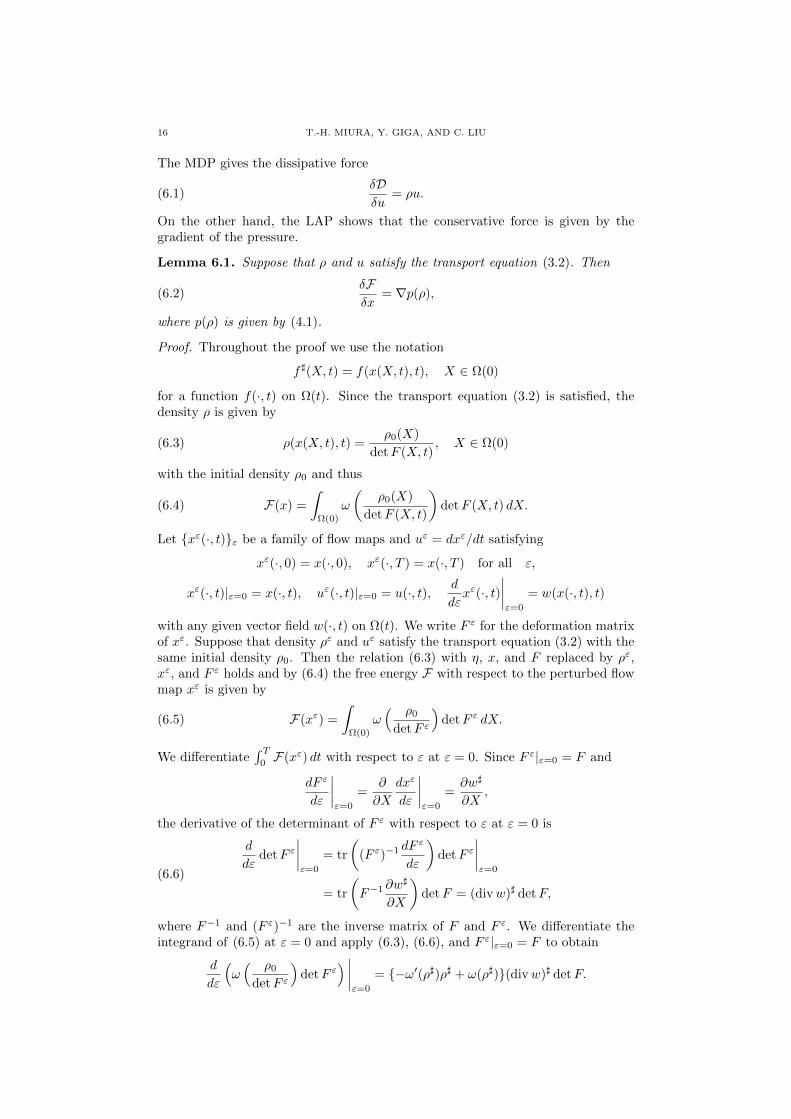
The MDP gives the dissipative force

δDδu

= ρu.(6.1)

On the other hand, the LAP shows that the conservative force is given by thegradient of the pressure.

Lemma 6.1. Suppose that ρ and u satisfy the transport equation (3.2). Then

δFδx

= ∇p(ρ),(6.2)

where p(ρ) is given by (4.1).

Proof. Throughout the proof we use the notation

f ](X, t) = f(x(X, t), t), X ∈ Ω(0)

for a function f(·, t) on Ω(t). Since the transport equation (3.2) is satisfied, thedensity ρ is given by

ρ(x(X, t), t) =ρ0(X)

detF (X, t), X ∈ Ω(0)(6.3)

with the initial density ρ0 and thus

F(x) =

∫Ω(0)

ω

(ρ0(X)

detF (X, t)

)detF (X, t) dX.(6.4)

Let xε(·, t)ε be a family of flow maps and uε = dxε/dt satisfying

xε(·, 0) = x(·, 0), xε(·, T ) = x(·, T ) for all ε,

xε(·, t)|ε=0 = x(·, t), uε(·, t)|ε=0 = u(·, t), d

dεxε(·, t)

∣∣∣∣ε=0

= w(x(·, t), t)

with any given vector field w(·, t) on Ω(t). We write F ε for the deformation matrixof xε. Suppose that density ρε and uε satisfy the transport equation (3.2) with thesame initial density ρ0. Then the relation (6.3) with η, x, and F replaced by ρε,xε, and F ε holds and by (6.4) the free energy F with respect to the perturbed flowmap xε is given by

F(xε) =

∫Ω(0)

ω( ρ0

detF ε

)detF ε dX.(6.5)

We differentiate∫ T

0F(xε) dt with respect to ε at ε = 0. Since F ε|ε=0 = F and

dF ε

dε

∣∣∣∣ε=0

=∂

∂X

dxε

dε

∣∣∣∣ε=0

=∂w]

∂X,

the derivative of the determinant of F ε with respect to ε at ε = 0 is

d

dεdetF ε

∣∣∣∣ε=0

= tr

((F ε)−1 dF

ε

dε

)detF ε

∣∣∣∣ε=0

= tr

(F−1 ∂w

]

∂X

)detF = (divw)] detF,

(6.6)

where F−1 and (F ε)−1 are the inverse matrix of F and F ε. We differentiate theintegrand of (6.5) at ε = 0 and apply (6.3), (6.6), and F ε|ε=0 = F to obtain

d

dε

(ω( ρ0

detF ε

)detF ε

) ∣∣∣∣ε=0

= −ω′(ρ])ρ] + ω(ρ])(divw)] detF.


Therefore,

d

dε

∫ T

0

F(xε) dt

∣∣∣∣ε=0

=

∫ T

0

∫Ω(0)

−ω′(ρ])ρ] + ω(ρ])(divw)] detF dX dt

=

∫ T

0

∫Ω(t)

−ω′(ρ)ρ+ ω(ρ)divw dxdt

=

∫ T

0

∫Ω(t)

∇[ω′(ρ)ρ− ω(ρ)] · w dxdt

and thus (6.2) follows.

By (6.1), (6.2), and K = 0, the balance of forces

δKδx

=δFδx

+δDδu

is of the form

0 = ∇p(ρ) + ρu, i.e., − ρu = ∇p(ρ),

which is exactly Darcy’s law in a moving domain. Combining this with the transportequation (3.2), we obtain the nonlinear diffusion equations

∂tρ+ div(ρu) = 0, −ρu = ∇p(ρ)

in the moving domain Ω(t), where p(ρ) is given by (4.1).From the above discussion, we expect that the energetic variational approach for

(5.2) yields Darcy’ law (4.10) on a moving surface. For (5.2), we have

K = 0, F =

∫Γ(t)

ω(η) dHn−1,

D =1

2

∫Γ(t)

η|vT |2 dHn−1, W =

∫Γ(t)

p(η)HV NΓ dHn−1.

The variation of D with respect to the total velocity v = V NΓ ν + vT gives

δDδv

= ηvT ,(6.7)

since vT = PΓv. Let us apply the LAP to the free energy F .

Lemma 6.2. Suppose that η and v of the form (4.8) satisfy the transport equation(3.5). Then

δFδy

= ∇Γp(η),(6.8)

where p(η) is given by (4.1).

We localize the integral over Γ(t) with a partition of unity of Γ(t) as in [13,Section 2.4] and take the variation of F with respect to a flow map in “local La-grangian coordinates.” Let y(·, t) : U → Γ(t) be a mapping defined on an open setU in Rn−1 such that

y(Y, 0) ∈ Γ(0),d

dty(Y, t) = v(y(Y, t), t), Y ∈ U.(6.9)

We consider a localized surface integral

F(y) =

∫y(U,t)

ω(η) dHn−1(6.10)


and take its variation with respect to y. Let yε(·, t)ε be a family of flow mapson Γ(t) in local Lagrangian coordinates, i.e. yε(·, t) : U → Γ(t) for each ε, anddyε/dt = vε such that

yε(·, 0) = y(·, 0), yε(·, T ) = y(·, T ) for all ε,

yε(·, t)|ε=0 = y(·, t), vε(·, t)|ε=0 = v(·, t), d

dεyε(·, t)

∣∣∣∣ε=0

= w(y(·, t), t)(6.11)

with any given tangential vector field w(·, t) on Γ(t). We use the notation

f ](Y, t) = f(y(Y, t), t), Y ∈ U(6.12)

for a function f(·, t) on Γ(t).

Lemma 6.3. Let g = (gij)i,j be a matrix given by

gij =∂y

∂Yi· ∂y∂Yj

, i, j = 1, . . . , n− 1(6.13)

and gε = (gεij)i,j be a matrix given as above with y replaced by yε. Then

d

dε

√det gε

∣∣∣∣ε=0

= (divΓw)]√

det g.(6.14)

Proof. Since gε|ε=0 = g and

d

dεdet gε = tr

((gε)−1 dg

ε

dε

)det gε,

where (gε)−1 is the inverse matrix of gε, we have

d

dε

√det gε

∣∣∣∣ε=0

=1

2tr

(g−1 dg

ε

dε

∣∣∣∣ε=0

)√det g,(6.15)

where g−1 = (gij)i,j is the inverse matrix of g. Moreover, since

dgεijdε

∣∣∣∣ε=0

=

(∂

∂Yi

dyε

dε· ∂y

ε

∂Yj+∂yε

∂Yj· ∂

∂Yj

dyε

dε

) ∣∣∣∣ε=0

=∂w]

∂Yi· ∂y∂Yj

+∂y

∂Yi· ∂w

]

∂Yj

for each i, j = 1, . . . , n−1, where we used the notation (6.12), and g−1 is symmetric,

tr

(g−1 dg

ε

dε

∣∣∣∣ε=0

)=

n−1∑i,j=1

gij(∂w]

∂Yi· ∂y∂Yj

+∂y

∂Yi· ∂w

]

∂Yj

)

= 2

n−1∑i,j=1

gij∂w]

∂Yi· ∂y∂Yj

= 2(divΓw)].

Substituting this for (6.15), we get (6.14).

Proof of Lemma 6.2. We first express the free energy F in “local Lagrangian co-ordinates.” Let U be an open set in Rn−1 and y(·, t) : U → Γ(t) be a flow mapsatisfying (6.9). For every open subset U ′ of U , the integral∫

U ′(t)

η(y, t) dHn−1(y) =

∫U ′η(y(Y, t), t)

√det g(Y, t) dY,

where U ′(t) = y(U ′, t), is constant in t, since η and v satisfy the transport equation(3.5). Hence

η(y(Y, t), t)√

det g(Y, t) = η(y(Y, 0), 0)√

det g(Y, 0), Y ∈ U(6.16)


and the localized surface integral (6.10) is expressed as

F(y) =

∫U

ω(η(y(Y, t), t))√

det g(Y, t) dY

=

∫U

ω

(η0(Y )√

det g(Y, t)

)√det g(Y, t) dY,

(6.17)

where η0(Y ) is given by the right-hand side of (6.16), where g is the function ofy = y(Y, t) as (6.13).

Next we take a variation of F with respect to the flow map y. Let yε(·, t)εbe a family of flow maps on Γ(t) in local Lagrangian coordinates satisfies (6.11).Suppose that density ηε and vε = dyε/dt satisfy the transport equation (3.5) andηε|t=0 = η|t=0 holds on yε(U, 0) = y(U, 0). Then the relation (6.16) with ηε, yε,and gε holds and by (6.17) the free energy F with respect to the perturbed flowmap yε is given by

F(yε) =

∫U

ω

(η0√

det gε

)√det gε dY.

Note that the right-hand side of (6.16) with ηε, yε, and gε is equal to η0(Y ) sinceηε|t=0 = η|t=0, yε|t=0 = y|t=0, and gε|t=0 = g|t=0. We differentiate the integrandof the right-hand side with respect to ε at ε = 0. Then by (6.14), (6.17), andgε|ε=0 = g we get

d

dε

(ω

(η0√

det gε

)√det gε

) ∣∣∣∣ε=0

= −ω′(η])η] + ω(η])(divΓw)]√

det g.

Here we used the notation (6.12). Hence

d

dε

∫ T

0

F(yε) dt

∣∣∣∣ε=0

=

∫ T

0

∫U

−ω′(η])η] + ω(η])(divΓw)]√

det g dY dt

=

∫ T

0

∫U(t)

−ω′(η)η + ω(η)divΓw dHn−1 dt

=

∫ T

0

∫U(t)

∇Γ[ω′(η)η − ω(η)] · w dHn−1 dt,

where U(t) = y(U, t). (Note that, since we localize the surface integral by using apartition of unity of Γ(t), we may assume the function ω′(η)η − ω(η) is compactlysupported in U(t).) Since w is an arbitrary tangential vector field on Γ(t), weconclude from the above equality that (6.8) holds.

By (6.7), (6.8), and K = 0, the balance of forces

δKδy

=δFδy

+δDδv

is of the form

0 = ∇Γp(η) + ηvT , i.e., − ηvT = ∇Γp(η),

which is Darcy’s law on a moving surface as we expected. Finally, combining thiswith the transport equation (3.5) we obtain the nonlinear equation

∂η − V NΓ Hη + divΓ(ηvT ) = 0,

−ηvT = ∇Γp(η)

on the moving surface Γ(t), where p(η) is given by (4.1).


Acknowledgments

The work of the first author was supported by JSPS through the Grant-in-Aidfor JSPS Fellows (No. 16J02664) and by MEXT through the Program for LeadingGraduate Schools. The work of the second author was partly supported by JSPSthrough the Grants Kiban S (No. 26220702) and Kiban B (No. 16H03948). Thework of the third author was partially supported by NSF grants DMS-141200 andDMS-1216938. A part of this work was done when the third author was visitingthe University of Tokyo in 2016.

References

[1] V. I. Arnol′d, Mathematical methods of classical mechanics, vol. 60 of Graduate Texts in

Mathematics, Springer-Verlag, New York, second ed., 1989. Translated from the Russian byK. Vogtmann and A. Weinstein.

[2] P. Cermelli, E. Fried, and M. E. Gurtin, Transport relations for surface integrals arising

in the formulation of balance laws for evolving fluid interfaces, J. Fluid Mech., 544 (2005),pp. 339–351.

[3] Q. Du, C. Liu, R. Ryham, and X. Wang, Energetic variational approaches in modeling

vesicle and fluid interactions, Phys. D, 238 (2009), pp. 923–930.[4] G. Dziuk and C. M. Elliott, Finite elements on evolving surfaces, IMA J. Numer. Anal.,

27 (2007), pp. 262–292.

[5] D. Gilbarg and N. S. Trudinger, Elliptic partial differential equations of second order,Classics in Mathematics, Springer-Verlag, Berlin, 2001. Reprint of the 1998 edition.

[6] M. E. Gurtin, An introduction to continuum mechanics, vol. 158 of Mathematics in Science

and Engineering, Academic Press, Inc. [Harcourt Brace Jovanovich, Publishers], New York-London, 1981.

[7] J. K. Hale and G. Raugel, A damped hyperbolic equation on thin domains, Trans. Amer.Math. Soc., 329 (1992), pp. 185–219.

[8] , Reaction-diffusion equation on thin domains, J. Math. Pures Appl. (9), 71 (1992),

pp. 33–95.[9] , A reaction-diffusion equation on a thin L-shaped domain, Proc. Roy. Soc. Edinburgh

Sect. A, 125 (1995), pp. 283–327.

[10] L. T. Hoang and G. R. Sell, Navier-Stokes equations with Navier boundary conditions foran oceanic model, J. Dynam. Differential Equations, 22 (2010), pp. 563–616.

[11] Y. Hyon, D. Y. Kwak, and C. Liu, Energetic variational approach in complex fluids: max-imum dissipation principle, Discrete Contin. Dyn. Syst., 26 (2010), pp. 1291–1304.

[12] D. Iftimie, G. Raugel, and G. R. Sell, Navier-Stokes equations in thin 3D domains with

Navier boundary conditions, Indiana Univ. Math. J., 56 (2007), pp. 1083–1156.[13] H. Koba, C. Liu, and Y. Giga, Energetic variational approaches for incompressible fluid

systems on an evolving surface, Quart. Appl. Math. , (2016).

[14] T.-H. Miura, Zero width limit of the heat equation on moving thin domains, Interfaces FreeBound. to appear.

[15] L. Onsager, Reciprocal relations in irreversible processes. I., Phys. Rev., 37 (1931), pp. 405–

426.[16] , Reciprocal relations in irreversible processes. II., Phys. Rev., 38 (1931), pp. 2265–

2279.[17] J. V. Pereira and R. P. Silva, Reaction-diffusion equations in a noncylindrical thin domain,

Bound. Value Probl., (2013), pp. 2013:248, 10.

[18] M. Prizzi, M. Rinaldi, and K. P. Rybakowski, Curved thin domains and parabolic equa-tions, Studia Math., 151 (2002), pp. 109–140.

[19] M. Prizzi and K. P. Rybakowski, The effect of domain squeezing upon the dynamics ofreaction-diffusion equations, J. Differential Equations, 173 (2001), pp. 271–320.

[20] M. Prizzi and K. P. Rybakowski, On inertial manifolds for reaction-diffusion equations ongenuinely high-dimensional thin domains, Studia Math., 154 (2003), pp. 253–275.

[21] G. Raugel, Dynamics of partial differential equations on thin domains, in Dynamical sys-tems (Montecatini Terme, 1994), vol. 1609 of Lecture Notes in Math., Springer, Berlin, 1995,

pp. 208–315.[22] G. Raugel and G. R. Sell, Navier-Stokes equations on thin 3D domains. I. Global attractors

and global regularity of solutions, J. Amer. Math. Soc., 6 (1993), pp. 503–568.[23] J. W. Strutt, Some general theorems relating to vibrations, Proceedings of the London

Mathematical Society, s1-4 (1871), pp. 357–368.


[24] H. Sun and C. Liu, On energetic variational approaches in modeling the nematic liquid

crystal flows, Discrete Contin. Dyn. Syst., 23 (2009), pp. 455–475.

[25] R. Temam and M. Ziane, Navier-Stokes equations in three-dimensional thin domains withvarious boundary conditions, Adv. Differential Equations, 1 (1996), pp. 499–546.

[26] , Navier-Stokes equations in thin spherical domains, in Optimization methods in partialdifferential equations (South Hadley, MA, 1996), vol. 209 of Contemp. Math., Amer. Math.

Soc., Providence, RI, 1997, pp. 281–314.

Graduate School of Mathematical Sciences, University of Tokyo, 3-8-1 Komaba,

Meguro-ku, Tokyo, 153-8914, JapanE-mail address: [email protected]

Graduate School of Mathematical Sciences, University of Tokyo, 3-8-1 Komaba,Meguro-ku, Tokyo, 153-8914, Japan

E-mail address: [email protected]

Department of Mathematics, Penn State University, University Park, PA 16802,

United States

E-mail address: [email protected]

introduction - 北海道大学eprints3.math.sci.hokudai.ac.jp/2409/1/pre1101.pdf · in summary, we...

Documents