introduction the ozone layer - university of richmondsabrash/110/ozonelayer-slides...introduction...

Introduction

Formation ofthe OzoneLayer

Depletion ofthe OzoneLayer

Ozone LayerRecovery

1 of 31

The Ozone LayerFormation, Depletion and Recovery

Introduction



Ozone LayerRecovery

2 of 31

Outline of Topics

1 IntroductionFunction of the Ozone LayerEffects of Ozone DepletionStructure of the Ozone Layer

2 Formation of the Ozone LayerThe Chapman CycleProblems with the Chapman Cycle

3 Depletion of the Ozone LayerCatalytic Destruction of OzoneCFC-induced DepletionComparison of Ozone SinksThe Ozone Hole

4 Ozone Layer RecoveryThe Montreal ProtocolGlobal Trends in Ozone

Introduction

Function of theOzone Layer

Effects of OzoneDepletion

Structure of theOzone Layer



Ozone LayerRecovery

3 of 31

What does the ozone layer do for us?

• 200-280 nm: UV-C (unaffected by O3 depletion)

• 280-320 nm: UV-B (O3 depletion affects this)

• 320-380 nm: UV-C (barely affected by O3 depletion)

Introduction






Ozone LayerRecovery

4 of 31

Give more detail on uv attenuation in the stratosphere.

• 50 km:λ > 185 nm

• Stronglyabsorbed near250 nm

• 200–210 nmpenetratesmore deeply

• 0 km:λ > 295 nm

Introduction






Ozone LayerRecovery

5 of 31

At what wavelengths does dioxygen, O2, attenuate light inthe atmosphere?

• note that y-axis is logarithmic in both plots

• absorbs strongly 130–170 nm

• absorbs weekly out to 205 nm

• absorption in Schumann-Runge bands is important in stratosphere

Introduction






Ozone LayerRecovery

6 of 31

How about absorption by ozone, O3? Why is it different thanabsorption by O2? What causes the stratospheric ‘spectralwindow?’

Dioxygen bonding O O

Ozone bonding OO

O OO

O

Introduction






Ozone LayerRecovery

7 of 31

So it filters out some uv light. Is that a big deal?

• B(λ) is the‘biological damagefunction’ of lighton DNA

• F (λ) is thepredicted lightintensity at twoO3 levels

• Product B(λ)F (λ)shows effect ofdepletion

Introduction






Ozone LayerRecovery

8 of 31

Lecture Question

Where is the ozone layer and how concentrated is it?

• left plot is (log) absolute conc, right is relative conc

• absolute more important for most purposes, max 25–30 km

• relative: O3 is 1–8 ppm, max at 35 km

Introduction


The ChapmanCycle

Problems withthe ChapmanCycle


Ozone LayerRecovery

9 of 31

Lecture Question

How is the stratospheric ozone layer formed?

Initiation: O2hν

2 O (λ ≤ 242 nm)

Cycling: O + O2 O3 + heat

Cycling: O3hν

O2 + O (λ ≤ 340 nm)

Termination: O3 + O 2 O2

Introduction


The ChapmanCycle



Ozone LayerRecovery

10 of 31

How does the Chapman cycle predict a stratospheric ozonelayer as well as the stratospheric thermal inversion?

• Rate of heating is det’d by rate of Ox cycling

• Heat is supplied by O3 photodissociation followed by O + O3

• Light is converted to heat• Controlled by rate of O3 photodissociation. Upper

stratosphere: 20 cycles/hr, lower stratosphere 1 cycle/hr.

• Conc of ozone (Ox) det’d largely by the source: rate of O2

photodissociation

• Depends on intensity of light 130–205 nm and absolute concof O2

• Mesosphere: lots of light but air is v thin• Troposphere: lots of O2 but no UV light below 295 nm

Introduction


The ChapmanCycle



Ozone LayerRecovery

11 of 31

Is the Chapman cycle correct? How could we evaluate it‘quantitatively’ (and what does that mean)?

• Qualitative agreement is notenough

• Quantitative: mustmeasure/predict reaction rates

• Off by factor of 2–4, dependingon altitude

Introduction


The ChapmanCycle



Ozone LayerRecovery

12 of 31

What’s wrong with the Chapman model and how can it befixed?

• Related: what does the term steady-state ozone mean (inthe previous figure)?

• Ox source too strong or sink too weak?

Introduction



CatalyticDestruction ofOzone

CFC-inducedDepletion

Comparison ofOzone Sinks

The Ozone Hole

Ozone LayerRecovery

13 of 31

What are the mechanisms that Chapman missed to destroyozone?

• Missing sink(s): catalytic destruction of Ox

• Why is it important that the destruction process becatalytic?

Introduction






The Ozone Hole

Ozone LayerRecovery

14 of 31

What are the catalytic species that deplete the ozone layer?

• Stratospheric NOx

• Stratospheric HOx

• Stratospheric ClOx and BrOx

Introduction






The Ozone Hole

Ozone LayerRecovery

15 of 31

Lecture Question

What are CFCs, and what are they used for?

• CFCs are chlorofluorocarbons: small molecules that contain Cl, Fand C atoms.

• Usually are only 1–2 carbon atoms

• Sometimes called Freons (trade name for DuPont)

• CFCs referred to by a number, most common are: CFC-11,CFC-12, CFC-113

• HCFCs are CFCs that contain hydrogen.

This makes them more reactive to the OH radical, decreasingtheir tropospheric lifetime. That means that, on apound-per-pound basis, HCFCs (’soft CFCs’) destroy lessstratospheric ozone than CFCs (‘hard CFCs’) because a smallerfraction of HCFCs reach the stratosphere.

Introduction






The Ozone Hole

Ozone LayerRecovery

16 of 31

What do the vertical concentration profiles of CFCs suggestabout their fate in the atmosphere?

• VMR is constant for the first 15 km or so (ie, the troposphere).What does this mean?

• Rate of removal of CFCs from the troposphere is slow:

• No photodissociation in troposphere• These CFCs do not react with OH• CFCs not water soluble

• Once in the stratosphere, rate of removal is faster than rate ofvertical mixing. Why?

Introduction






The Ozone Hole

Ozone LayerRecovery

17 of 31

What are the tropospheric sources of stratospheric chlorine?

CFC-11: CFCl3CFC-12: CF2Cl2CFC-113: CF3CCl3

HCFC-22: CHF2Cl

• More than 80% of stratospheric Cl is anthropogenic

• HCl is very water soluble

Introduction






The Ozone Hole

Ozone LayerRecovery

18 of 31

Lecture Question

Let’s put it all together: how do CFCs deplete the strato-spheric ozone layer? Explain in detail.

1. CFC discharged to the troposphere

2. After 5–10 yr, CFCs enter the stratosphere

3. Soon after entering the stratosphere they photodissociate.

CFCl3hν

CFCl2 + Cl (λ ≤ 225 nm)

4. Cl atoms destroy Ox catalytically

Cl + O3 ClO + O2

ClO + O Cl + O2

net: O3 + O 2 O2

Introduction






The Ozone Hole

Ozone LayerRecovery

19 of 31

What are the sources of stratospheric NOx , HOx , and BrOx?How much is due to human activity?

Q.17

Figure Q7-1. Stratospheric source gases. A variety of halogen source gases emitted from natural sources and by human activities transport chlorine and bromine into the stratosphere . Ozone-depleting substances (ODSs) are the subset of these gases emitted by human activities that are controlled by the Montreal Protocol . These partitioned columns show the sources and abundances of chlorine- and bromine-containing gases entering the stratosphere in 2008 . The approximate amounts are derived from tropospheric observations of each gas in 2008 . Note the large difference in the vertical scales: total chlorine entering the stratosphere is 150 times more abundant than total bromine . Human activities are the largest source of chlorine reaching the stratosphere and the CFCs are the most abundant chlorine-containing gases . Methyl chloride is the primary natural source of chlorine . HCFCs, which are substitute gases for CFCs and also controlled under the Montreal Protocol, are a small but growing fraction of chlorine-containing gases . For bromine entering the stratosphere, halons and methyl bromide are the largest contributors . Methyl bromide has an additional, much larger, natural source . Natural sources provide a much larger fraction of total bromine entering the stratosphere than of total chlorine . (The unit “parts per trillion” is used here as a measure of the relative abundance of a gas in air: 1 part per trillion equals the presence of one molecule of a gas per trillion (=1012) total air molecules .)

Lifetimes and emissions . After emission, halogen source gases are either naturally removed from the atmosphere or undergo chemical conversion in the troposphere or strato-sphere. The time to remove or convert about 60% of a gas is often called its atmospheric lifetime. Lifetimes vary from less than 1 year to 100 years for the principal chlorine- and bromine-containing gases (see Table Q7-1). The long-lived gases are primarily destroyed in the stratosphere and essen-tially all of the emitted halogen is available to participate in the destruction of stratospheric ozone. Gases with the short lifetimes (e.g., the HCFCs, methyl bromide, methyl chloride, and the very short-lived gases) are substantially destroyed in the troposphere and, therefore, only a fraction of the emitted halogen contributes to ozone depletion in the stratosphere.

The amount of an emitted gas that is present in the atmo-

sphere represents a balance between the emission rate and the lifetime of the gas. Emission rates and atmospheric lifetimes vary greatly for the source gases, as indicated in Table Q7-1. For example, the atmospheric abundances of most of the principal CFCs and halons have decreased since 1990 while those of the leading substitute gases, the hydrochlorofluoro-carbons (HCFCs), continue to increase under the provisions of the Montreal Protocol (see Q16). In the coming decades, the emissions and atmospheric abundances of all controlled gases are expected to decrease under these provisions.

Ozone Depletion Potential (ODP). Halogen source gases are compared in their effectiveness to destroy stratospheric ozone using the ODP, as listed in Table Q7-1 (see Q18). A gas with a larger ODP destroys more ozone over its atmospheric lifetime. The ODP is calculated relative to CFC-11, which has

Section II: THE OZONE DEPLETION PROCESS 20 Questions: 2010 Update

Chlorine source gases Bromine source gases

1000

2000

30003320

016.6%

CFC-12 (CCl2F2)32.3%

CFC-11 (CCl3F)

Carbon tetrachloride (CCl4)10.8%

22%

Methyl chloroform (CH3CCl3) 1%

Methyl chloride (CH3Cl)

Other gases 2.9%

10

20

0

Other gases 4.3%21.6

15

5

HCFCs (e.g., HCFC-22 = CHClF2)7.5%CFC-113 (CCl2FCClF2)6.9%

Very short-lived gases(e.g., bromoform = CHBr3)

27.8%

29.8%

Halon-1211 (CBrClF2)19.3%

Halon-1301 (CBrF3)14.7%

4.1%

Hum

an-a

ctivi

ty s

ourc

es

Ozo

ne-d

eple

ting

subs

tanc

es (O

DSs)

Hum

an-a

ctivi

tyso

urce

s

ODS

s

Naturalsources

Natu

ral s

ourc

es

Halogen Source Gases Entering the Stratosphere in 2008

Tota

l chl

orin

e am

ount

(par

ts p

er tr

illion

)

Tota

l bro

min

e am

ount

(par

ts p

er tr

illion

)

Methyl bromide(CH3Br)

• Stratospheric BrOx shown infigure; 40–45% increase in BrOx

due to human activities.

• Stratospheric NOx

Source is tropospheric N2O.15–20% increase due to humanactivities. Use of nitrogenousfertilizers and fossil fuelcombustion are the main causes.

• Stratospheric HOx

Sources: tropospheric CH4, H2,H2O. 150% increase in CH4 due toa variety of human activities.

Introduction






The Ozone Hole

Ozone LayerRecovery

20 of 31

How do the different mech-anisms of ozone depletioncompare?

• Ox is Chapman:O3 + O 2 O2.Never the dominantmechanism.

• NOx is dominant inmiddle stratosphere,HOx in lower andupper.

• ClOx is significant butnever dominant, BrOx

is even less.

Introduction






The Ozone Hole

Ozone LayerRecovery

21 of 31

How do the different mechanisms of ozone depletioncompare?

Above are absolute rates. Approx 60% of all loss due to NOx , 20%due to Chapman, 20% due to all others.

Introduction






The Ozone Hole

Ozone LayerRecovery

22 of 31

Lecture Question

What is the ozone hole and where does it form?

• Left: O3 hole for Sept 2006

• The ozone hole is the regionover Antarctica withTCO < 220 DU.

• 1 DU is equivalent to 10 µmat STP

• Typical TCO is 300 DU

Introduction






The Ozone Hole

Ozone LayerRecovery

23 of 31

Lecture Question

Is the ozone hole a permanent feature of the Antarctic? Ifnot, when does it form?

The ozone hole appears soon after the sun rises in the spring (thereis no sun in the polar winter).

Introduction






The Ozone Hole

Ozone LayerRecovery

24 of 31

Lecture Question

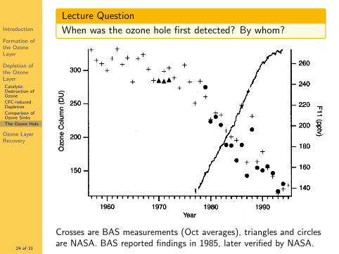
When was the ozone hole first detected? By whom?

Crosses are BAS measurements (Oct averages), triangles and circlesare NASA. BAS reported findings in 1985, later verified by NASA.

Introduction






The Ozone Hole

Ozone LayerRecovery

25 of 31

Lecture Question

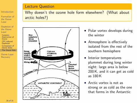
Why doesn’t the ozone hole form elsewhere? (What aboutarctic holes?)

• Polar vortex develops duringthe winter

• Atmosphere is effectivelyisolated from the rest of thesouthern hemisphere

• Interior temperaturesplummet during long winternight: large area is below200 K, and it can get as coldas 180 K

• Arctic vortex is not asstrong or as cold as the onethat forms in the Antarctic

Introduction






The Ozone Hole

Ozone LayerRecovery

26 of 31

Do we know that stratospheric chlorine from CFCs is respon-sible for the ozone hole?

The above ‘smoking gun’ measurement was part of a conclusive bodyof research conducted in 1985–1989 showing ozone holes were due tostratospheric Cl and Br.

Introduction






The Ozone Hole

Ozone LayerRecovery

27 of 31

Lecture Question

So how does the ozone hole form?

Introduction



Ozone LayerRecovery

The MontrealProtocol

Global Trends inOzone

28 of 31

Lecture Question

What treaty was signed to control ozone depletion, and whendid it go into effect? How effective has it been in controllingstratospheric chlorine levels?

10

Emissions from the current banks (in 2015) over the next 35 years are projected to contribute more to ozone depletion over the coming few decades than emissions associated with future ODS production, assuming compliance with the Montreal Protocol (Figure ADM 1-4). The halon and CFC banks are projected to contribute roughly equally to future ozone depletion. However, the halon banks are more amenable to recapture than the CFC banks.8 Capture and destruction of CFC, halon, and HCFC banks could avoid 1.8 million ODP-tonnes of future emission through 2050, while the future production could contribute roughly 0.85 million ODP-tonnes, assuming compliance with the Protocol. These values are to be compared with an estimated 1.6 million ODP-tonnes of emissions from banks between 2005–2014.

Midlatitude EESC, the metric used to estimate the extent of chemical ozone layer depletion, will return to its 1980 values between 2040 and 2060 (see Figure ADM 1-3). Model simulations that take into account the effects on ozone from ODSs and GHGs provide estimates for return dates of total column ozone abundances to 1980 levels. These calculated ranges of dates within which we expect the return of ozone to 1980 values have not changed since the last Assessment. They are:

• 2025 to 2040 for global mean annually averaged ozone (see Fig. ADM 1-5)

• 2030 to 2040 for annually averaged Southern Hemisphere midlatitude ozone

• 2015 to 2030 for annually averaged Northern Hemisphere midlatitude ozone

• 2025 to 2035 for springtime Arctic ozone (see Figure ADM 1-6)

• 2045 to 2060 for springtime Antarctic ozone (see Figure ADM 1-6)

Highlight 1-6

Total column ozone will recover toward the 1980 benchmark levels over most of the globe under continued compliance with the Montreal Protocol. [Chapter 2: Sections 2.4 and 2.5]

CCl4

CH Br3

HCFCs

halons

CFCs

HCFCs

HCFCs

2.0

0.8

0.4

1.2

1.6

0.0Production 2015 Banks

Mill

ions

of O

DP-

Wei

ghte

d To

nnes

Figure ADM 1-4. A comparison of the cumulative projected emissions from current banks of the CFCs, halons, and HCFCs between 2015 and 2050 with the cumulative projected emissions from production of ODSs during the same period.

-6

-3

0

3

6

Tota

l Ozo

ne C

olum

n Ch

ange

(%)

Models ±2σ

Observations

1960

0

1000

2000

EESC

(ppt

)

Equivalent EffectiveStratospheric Chlorine

total ozone column 60°S-60°N

2000 2040 2080

1960 2000 2040 2080

Figure ADM 1-5. Top Panel: Variation in EESC at midlatitudes between 1960 and 2100. The future EESC is for the baseline scenario (described in the text before Highlight 1-1). Bottom panel: The average total column ozone changes over the same period, from multiple model simulations (see Chapter 2), are shown as a solid gray line. This is compared with the observed column ozone changes between 1965 and 2013 (blue line), the period for which observations are available.

8 IPCC-TEAP Special Report, Safeguarding the Ozone Layer and the Global Climate System: Issues Related to Hydrofluorocarbons and Perfluorocarbons, Cambridge University Press, Cambridge, U.K., 488 pp., 2005.

• The MontrealProtocol wassigned in 1987and went intoeffect in 1989

• Regulated CFCsand HCFCsseparately

• Phase-outschedules relaxedfor LDCs

• Stratospheric Cllevels have beendecreasing sincethe late 1990s.

Introduction



Ozone LayerRecovery



29 of 31

Lecture Question

What treaty was signed to control ozone depletion, and whendid it go into effect? How effective has it been in controllingstratospheric chlorine levels?

Q.46

20 Questions: 2010 Update Section IV: CONTROLLING OZONE-DEPLETING SUBSTANCES

ful UV-B radiation would have increased substantially at Earth’s surface, causing a global rise in skin cancer and cataract cases (see Q17).

▶ Montreal Protocol provisions. International compliance with only the 1987 provisions of the Montreal Protocol and the later 1990 London Amendment would have sub-stantially slowed the projected growth of EESC. Not until the 1992 Copenhagen Amendments and Adjustments did the Protocol projections show a decrease in future EESC values. The provisions became more stringent with the Amendments and Adjustments adopted in Beijing in 1999 and Montreal in 1997 and 2007. Now, with full compli-ance to the Protocol, most ODSs will be almost completely phased out, with some exemptions for critical uses (see Q16). Global EESC is slowly decaying from its peak value in the late 1990s and is expected to reach 1980 values in the mid-21st century. The success of the Montreal Protocol to date is demonstrated by the decline in ODP-weighted emissions of ODSs shown in Figure Q0-1. Total emissions peaked in 1988 at values about 10-fold higher than natural

emissions. Between 1988 and 2010, ODS emissions from human activities have decreased by over 80%.

▶ Zero emissions. EESC values in the coming decades will be influenced by (1) the slow natural removal of ODSs still present in the atmosphere, (2) emissions from continued production and use of ODSs, and (3) emissions from cur-rently existing banks containing a variety of ODSs. ODS banks are associated with applications that involve long-term containment of halogen gases. Examples are CFCs in refrigeration equipment and insulating foams, andhalons in fire-fighting equipment. New emissions are pro-jected based on continued production and consumption ofODSs, particularly in developing nations, under existing Protocol provisions.

The zero-emissions case demonstrates the EESC values that would occur if it were possible to set all ODS emis-sions to zero beginning in 2011. This would eliminate the contributions from new production and bank emissions. Significant differences from the Montreal 2007 projections are evident in the first decades following 2011 because the

Figure Q15-1. Effect of the Montreal Protocol. The objective of the Montreal Protocol is the pro-tection of the ozone layer through control of the global production and consumption of ODSs . Projections of the future abundances of ODSs expressed as equivalent effective stratospheric chlorine (EESC) values (see Q16) are shown separately for the midlatitude stratosphere for (1) no Protocol provisions, (2) the provisions of the original 1987 Montreal Protocol and some of its subsequent Amendments and Adjust-ments, and (3) zero emissions of ODSs starting in 2011 . The city names and years indicate whereand when changes to the original 1987 Protocol provisions were agreed upon (see Figure Q0-1) . EESC is a relative measure of the potential for stratospheric ozone depletion that combinesthe contributions of chlorine and bromine from ODS surface observations (see Q16) . Without the Protocol, EESC values are projected to haveincreased significantly in the 21st century . Only with the Copenhagen (1992) and subsequentAmendments and Adjustments did projected EESC values show a long-term decrease .

198019600

2000 2020 2040 2060 2080 2100Year

Montreal1987

London1990

Beijing1999

Montreal2007

Zero Emissionsin 2011

Copenhagen1992

No Protocol

EESC

(rel

ativ

e am

ount

s)

Effect of the Montreal ProtocolLong-term changes in equivalent effective

stratospheric chlorine (EESC)

Natural sources

1

3

2

4

• Montreal Protocol could berevised as new scientificevidence was discovered

• Results/projections oforiginal treaty and ofrevisions on stratospheric Clshown in the figure

Introduction



Ozone LayerRecovery



30 of 31

Lecture Question

How severe has stratospheric ozone depletion been in the mid-latitudes? When is it expected to recover?

Chapter 2

2.50

Increasing methane, on the other hand, will generally increase ozone levels by tying up chlorine and by enhancing ozone production in the lower stratosphere. In the second half of the century, lower chlorine levels, stratospheric cooling, and other factors will reduce the efficiency by which CH4 and N2O emissions affect ozone. Continued monitoring Apart from future ODS levels, future levels of GHGs, especially carbon dioxide (CO2), nitrous oxide (N2O), methane (CH4), and water vapor (H2O) are expected to have important effects on the evolution of stratospheric ozone. Although most scenarios predict a recovery of stratospheric ozone, only continued measurements of ozone and these trace gases, and the combination of observations and model simulations, can verify that the ozone layer is recovering.

1960 2000 2040 2080

-4

0

4

8oz

one

anom

aly

[%]

CCMVal-2 ±2Vobservations

total ozone column 60°S to 60°N

Figure 2-26. Simulated and observed evolution of the near global total ozone column. Observations are annual mean anomalies averaged over all available ground- and satellite-based measurements (blue line). Black line and gray range give multi-model mean and ±2 standard deviations of simulated individual model annual mean anomalies for the CCMVal-2 simulations already used in WMO (2011). Only the subset of 9 models performing runs for fixed ODS and for all forcings is used. All data are referenced to the 1998 to 2008 period. Up to 2000, the simulations account for changing ODSs, GHGs, observed sea surface temperatures and sea ice, volcanic aerosol, the 11-year solar-cycle, and the QBO (REF-B1 scenario, Eyring et al., 2010; WMO, 2011). After 2000 the adjusted A1 scenario of WMO (2007) is used for ODSs, the SRES A1B scenario is used for GHGs, sea surface temperatures and sea ice are from other models, the QBO is generated internally, there is no volcanic aerosol, and most models, except for 3, do not include the solar cycle (REF-B2 scenario, Eyring et al., 2010; WMO, 2011).

Introduction



Ozone LayerRecovery



31 of 31

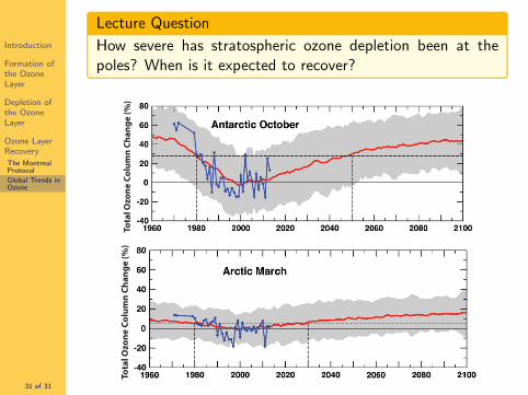
Lecture Question

How severe has stratospheric ozone depletion been at thepoles? When is it expected to recover?

11

Tropical column ozone is projected by models to remain below 1980s values over the coming decades because of a strengthened Brewer-Dobson circulation (see Box ADM 3-1, page 21) from tropospheric warming due to increased greenhouse gases (see Highlight 3-4), which acts to decrease ozone in the tropical lower stratosphere.

Model results suggest that global stratospheric ozone depletion due to ODSs did occur prior to 1980. The midlatitude EESC wasabout 570 ppt in 1960 and nearly 1150 ppt by 1980 (see Figure ADM 1-3). The 1980 baseline for ozone recovery was chosen, as in the pastAssessments, based upon the onset of a discernible decline in observed global total column ozone. Between 1960 and 1980, the depletionwas not large enough to be clearly distinguishable from the year-to-year variability, especially given the sparsity of observations. If the 1960value were chosen as the baseline, the EESC would return to that value well after 2100 (see Figure ADM 1-3 and Figure ADM 1-5 top panel).

Box ADM 1-2: Climate Metrics

There are many metrics used to measure the influence of a chemical or an emission on the climate system. The choice of metric depends on the issue being addressed. The most common of these metrics are: (1) radiative forcing (RF); (2) Global Warming Potential (GWP); (3) GWP-weighted emissions; and (4) Global Temperature change Potential (GTP). These four metrics are briefly described below in simple terms. Further details can be found in the “Additional Information of Interest to Decision-Makers” section of this document, as well as Chapter 5 of this 2014 Assessment and references therein.

Radiative Forcing (RF): This is a measure of the change in the radiation flux from the troposphere due to the presence of a greenhouse gas (GHG) in the atmosphere. There are various constraints on how this is calculated. RF is not an observed quantity, but can be estimated from the molecular properties and atmospheric abundance of the GHG, and atmospheric properties. This metric allows comparison of different forcing agents and is based on there being a clear relationship between the globally averaged radiative forcing and the globally averaged annual mean surface temperature.

Global Warming Potential (GWP): This represents the climate effect from a pulse emission of a GHG by integrating the radiative forcing over a specific time interval and comparing it to the integrated forcing by emissions of the same weight of CO2. It is a relative measure, very roughly speaking, of the total energy added to the climate system by a component under consideration relative to that added by CO2 over the time period of the chosen time horizon. The choice of the time horizon is based on policy choices. The most common choice is 100 years. In this report, the 100-year GWP (GWP100) is used unless specified otherwise. GWP is the most widely used metric for assessing the climate impact of GHGs.

GWP-Weighted Emissions (gigatonnes CO2-equivalent): This quantity is the product of the mass of a substance emitted and its GWP100

and expressed in gigatonnes CO2-equivalent. This product yields a simple measure of the future time-integrated climate impact of an emission.

Global Temperature change Potential (GTP): This is a relative measure of the temperature increase at a specific time horizon per unit mass pulse emission of a GHG relative to that for the emission of the same mass of CO2. This quantity is calculated using climate models. As in the case of GWPs, GTPs can be calculated for any time horizon of choice. This metric is not used in the current Assessment, but is used in the recent IPCC Assessment. Readers are referred to the IPCC Assessment 9 for the GTP values. GTP-weighted emissions are also calculated by multiplying the mass of emission by the GTP of that gas.

Tota

l Ozo

ne C

olum

n Ch

ange

(%)

Figure ADM 1-6. Total column ozone changes for the Arctic in March (left) and Antarctic in October (right). The red line is the model average, while gray shading shows the model range (±2σ) (see Chapter 3). Satellite observations are shown in blue. This figure is a composite adaption of Figure 3-16 of Chapter 3 for the model output and Figure 3-4 of Chapter 3 for the observations.

9 IPCC AR5, Climate Change 2013: The Physical Science Basis, Contribution of Working Group I to the Fifth Assessment Report of the Intergovernmental Panel on Climate Change, Cambridge University Press, 1535 pp., 2013.

11

Tropical column ozone is projected by models to remain below 1980s values over the coming decades because of a strengthened Brewer-Dobson circulation (see Box ADM 3-1, page 21) from tropospheric warming due to increased greenhouse gases (see Highlight 3-4), which acts to decrease ozone in the tropical lower stratosphere.

Model results suggest that global stratospheric ozone depletion due to ODSs did occur prior to 1980. The midlatitude EESC was about 570 ppt in 1960 and nearly 1150 ppt by 1980 (see Figure ADM 1-3). The 1980 baseline for ozone recovery was chosen, as in the past Assessments, based upon the onset of a discernible decline in observed global total column ozone. Between 1960 and 1980, the depletion was not large enough to be clearly distinguishable from the year-to-year variability, especially given the sparsity of observations. If the 1960 value were chosen as the baseline, the EESC would return to that value well after 2100 (see Figure ADM 1-3 and Figure ADM 1-5 top panel).

Box ADM 1-2: Climate Metrics

There are many metrics used to measure the influence of a chemical or an emission on the climate system. The choice of metric depends on the issue being addressed. The most common of these metrics are: (1) radiative forcing (RF); (2) Global Warming Potential (GWP); (3) GWP-weighted emissions; and (4) Global Temperature change Potential (GTP). These four metrics are briefly described below in simple terms. Further details can be found in the “Additional Information of Interest to Decision-Makers” section of this document, as well as Chapter 5 of this 2014 Assessment and references therein.

Radiative Forcing (RF): This is a measure of the change in the radiation flux from the troposphere due to the presence of a greenhouse gas (GHG) in the atmosphere. There are various constraints on how this is calculated. RF is not an observed quantity, but can be estimated from the molecular properties and atmospheric abundance of the GHG, and atmospheric properties. This metric allows comparison of different forcing agents and is based on there being a clear relationship between the globally averaged radiative forcing and the globally averaged annual mean surface temperature.

Global Warming Potential (GWP): This represents the climate effect from a pulse emission of a GHG by integrating the radiative forcing over a specific time interval and comparing it to the integrated forcing by emissions of the same weight of CO2. It is a relative measure, very roughly speaking, of the total energy added to the climate system by a component under consideration relative to that added by CO2 over the time period of the chosen time horizon. The choice of the time horizon is based on policy choices. The most common choice is 100 years. In this report, the 100-year GWP (GWP100) is used unless specified otherwise. GWP is the most widely used metric for assessing the climate impact of GHGs.

GWP-Weighted Emissions (gigatonnes CO2-equivalent): This quantity is the product of the mass of a substance emitted and its GWP100 and expressed in gigatonnes CO2-equivalent. This product yields a simple measure of the future time-integrated climate impact of an emission.

Global Temperature change Potential (GTP): This is a relative measure of the temperature increase at a specific time horizon per unit mass pulse emission of a GHG relative to that for the emission of the same mass of CO2. This quantity is calculated using climate models. As in the case of GWPs, GTPs can be calculated for any time horizon of choice. This metric is not used in the current Assessment, but is used in the recent IPCC Assessment. Readers are referred to the IPCC Assessment 9 for the GTP values. GTP-weighted emissions are also calculated by multiplying the mass of emission by the GTP of that gas.

Tota

l Ozo

ne C

olum

n Ch

ange

(%)

Figure ADM 1-6. Total column ozone changes for the Arctic in March (left) and Antarctic in October (right). The red line is the model average, while gray shading shows the model range (±2σ) (see Chapter 3). Satellite observations are shown in blue. This figure is a composite adaption of Figure 3-16 of Chapter 3 for the model output and Figure 3-4 of Chapter 3 for the observations.

9 IPCC AR5, Climate Change 2013: The Physical Science Basis, Contribution of Working Group I to the Fifth Assessment Report of the Intergovernmental Panel on Climate Change, Cambridge University Press, 1535 pp., 2013.

introduction the ozone layer - university of richmondsabrash/110/ozonelayer-slides...introduction...

Documents