introduction to advanced mathematics pete l. clark

Introduction to Advanced Mathematics

Pete L. Clark

Contents

Chapter 1. Sets 71. Introducing Sets 72. Subsets 123. Power Sets 134. Operations on Sets 135. Families of Sets 156. Partitions 177. Cartesian Products 188. Exercises 20

Chapter 2. Logic 231. Statements 232. Logical Operators 243. Logical Equivalence, Tautologies and Contradictions 264. Implication 275. The Logic of Contradiction 306. Logical Expressions Revisited 307. Open Sentences and Quantifiers 338. Negating Statements 399. Exercises 43

Chapter 3. Counting Finite Sets 451. Cardinality of a Finite Union 452. Independent Choices and Cartesian Products 483. Counting Irredundant Lists and Subsets 514. The Binomial Theorem 535. The Inclusion-Exclusion Principle 556. The Pigeonhole Principle 587. Exercises 60

Chapter 4. Number Systems 631. Field Axioms for R 632. Well-Ordering 65

Chapter 5. Number Theory 691. The Division Theorem 692. Divisibility 703. Infinitely Many Primes 724. Greatest Common Divisors 735. The GCD as a Linear Combination 76

3

4 CONTENTS

6. Euclid’s Lemma 787. The Least Common Multiple 798. The Fundamental Theorem of Arithmetic 819. Exercises 82

Chapter 6. Fundamentals of Proof 851. Vacuously True and Trivially True Implications 852. Direct Proof 873. Contrapositive 884. Contradiction 885. Without Loss of Generality 886. Biconditionals and Set Equality 88

Chapter 7. Induction 891. Introduction 892. The (Pedagogically) First Induction Proof 913. The (Historically) First(?) Induction Proof 924. Closed Form Identities 945. More on Power Sums 956. Inequalities 977. Extending binary properties to n-ary properties 998. Miscellany 1019. One Theorem of Graph Theory 10110. The Principle of Strong/Complete Induction 10411. Solving Homogeneous Linear Recurrences 10612. The Well-Ordering Principle 10913. Upward-Downward Induction 11014. The Fundamental Theorem of Arithmetic 11215. Exercises 115

Chapter 8. Relations and Functions 1171. Relations 1172. Equivalence Relations 1223. Composition of Relations 1244. Functions 1245. Exercises 132

Chapter 9. Countable and Uncountable Sets 1351. Introducing equivalence of sets, countable and uncountable sets 1352. Some further basic results 1413. Some final remarks 1444. Exercises 145

Chapter 10. Order and Arithmetic of Cardinalities 1471. The fundamental relation ≤ 1472. Addition of cardinalities 1493. Subtraction of cardinalities 1504. Multiplication of cardinalities 1515. Cardinal Exponentiation 1526. Note on sources 155

CONTENTS 5

7. Exercises 155

Chapter 11. Well-Ordered Sets, Ordinalities and the Axiom of Choice 1571. The Calculus of Ordinalities 1572. The Axiom of Choice and some of its equivalents 1703. Exercises 174

Bibliography 175

CHAPTER 1

Sets

1. Introducing Sets

Sets are the first of the three languages of mathematics. They are the most basickind of mathematical structure; all other structures are built out of them.1

A set is a collection of mathematical objects. This is not a careful definition;it is an informal description meant to convey the correct intuition.

1.1. Many Examples. We begin with some familiar examples.

Example 1.1. One can think of a set as a kind of club; some things are mem-bers; some things are not. So for instance current UGA students form a set. Youare a member; I am not. Past or present presidents of the United States form aset. Barack Obama is a member. Hillary Clinton is not.

Example 1.2. For any whole number n ≥ 1, {1, 2, . . . , n} is a set, whoseelements are indeed 1, 2, 3, . . . , n. Let us denote this set by [n]. So for instance

5 ∈ [9] = {1, 2, 3, 4, 5, 6, 7, 8, 9}

and

9 /∈ [5] = {1, 2, 3, 4, 5}.(For whole numbers a, b ≥ 1, we have a ∈ [b] precisely when a ≤ b.)

Example 1.3. The positive integers

Z+ = {1, 2, 3, . . .}

are a set. The positive integer 1 is an element, or member of Z+: we write thisstatement as

1 ∈ Z+.

So is the positive integer 2: we write

2 ∈ Z+.

Similarly,

3 ∈ Z+, 4 ∈ Z+, and so forth.

1Like most broad, sweeping statements made at the beginning of courses, this one is not

completely true. Mathematics is at least 2500 years old: Pythagoras died circa 495 BCE. Thepractice of describing all mathematical objects in terms of sets dates from approximately 1900.

Many mathematicians have at least contemplated basing mathematics on other kinds of objects;

something called “categories,” first introduced in the 1940’s by Eilenberg and Mac Lane, havelong had a significant (though minority) popularity. Nevertheless every student or practitioner of

mathematics must speak the language of sets, which is what we are now introducing.

7

8 1. SETS

The negative integer −3 is not an element of Z+. We write this as

−3 /∈ Z+.

The integer 0, which is not positive (this is an explanation of terminology, not amathematical fact), is not a member of Z+:

0 /∈ Z+.

Also 45 /∈ Z,

√2 /∈ Z+ and Barack Obama /∈ Z+. Of course lots of things are not

in Z+: we had better move on.

Example 1.4. The non-negative integers, or natural numbers

N = {0, 1, 2, 3, . . . , }are a set. The only difference between Z+ and N is that 0 ∈ N whereas 0 /∈ Z+.(This may seem silly, but it is actually useful to have both Z+ and N around.)

Example 1.5. The integers, both positive and negative

Z = {. . . ,−3,−2,−1, 0, 1, 2, 3, . . .}form a set. This time −3 ∈ Z, but still 4

5 /∈ Z,√

2 /∈ Z and Barack Obama /∈ Z.

Example 1.6. A rational number is a quotient of two integers ab with b 6= 0.

Rational numbers have many such representations, but ab = c

d exactly when ad = bc.

The rational numbers form a set, denoted Q.√

2 /∈ Q (this is an important theoremof ancient Greek mathematics that we will discuss later); Barack Obama /∈ Q.

Example 1.7. The real numbers form a set, denoted R. A real number can berepresented as an integer followed by an infinite decimal expansion. Still BarackObama /∈ R.

Example 1.8. A complex number is an expression of the form a+ bi, wherea, b ∈ R and i2 = −1. The set of complex numbers is denoted by C. i is a member;still Barack Obama /∈ C.

Actually, apart from Example 1, Barack Obama is not going to be a member ofany of the sets we will introduce. (Nor Mitt Romney, nor Olivia Rodrigo, nor...)To be honest, although we insisted that anything can be an element of a set, inmathematics – apart from preliminary discussions of exactly the sort you have justseen – we only consider sets that contain as members mathematical objects.

On the one hand, this is not surprising because mathematics is, obviously,the study of mathematical things. On the other hand, the notion of a “non-mathematical object” brings some philosophical difficulties. In particular, sincesets contain objects without any notion of multiplicity, in order to form a set, giventwo objects x and y, we need to have a clean answer to the question “Does x = y?”When considering identity of non-mathematical objects we are drawn into delicateissues of spatio-temporal continuity.2

We did not begin by saying that “A set is a collection of mathematical objects”because we were not – and are still not now – ready to address the natural followupquestion “What is a mathematical object?” But here is a taste of a kind of answer:

2E.g.: is the you of 2021 the same person as the you of 2005? Your atoms are different. If

a worm is divided into two, are the old worm and the two new worms one, two or three differentobjects? And so forth. These are fun questions, but not they have absolutely nothing to do with

mathematics.

1. INTRODUCING SETS 9

Any set of mathematical objects is itself a mathematical object. For now this prob-ably sounds both circular and insufficient. It turns out that neither of those thingsis true. You may – or may not; it’s by no means necessary – understand why a bitbetter by the end of the course.

Example 1.9. The Euclidean plane forms a set, denoted R2. Its elements arethe points in the plane, i.e., ordered pairs (x, y) with x, y real numbers: we writex, y ∈ R. For a positive integer n, n-dimensional Euclidean space forms a set,whose elements are ordered tuples (x1, . . . , xn) of real numbers. It is denoted Rn.

Example 1.10. Here are some examples from geometry / linear algebra:

a) The lines ` in the Euclidean plane R2 form a set.b) The planes P in Euclidean space R3 form a set.

Example 1.11. The continuous functions f : [0, 1]→ R form a set.

Some of these examples were an excuse to introduce common mathematicalnotation. But I hope the idea of a set is clear by now: it is a collection of (for us:mathematical!) objects. Practically speaking, this amounts to the following: if Sis a set and x is any object, then exactly one of the following must hold: x ∈ S orx /∈ S. That’s the point of a set: if you know exactly what is and is not a memberof a set, then you know the set. Thus a set is like a bag of objects...but not a redbag or a cloth bag. The bag itself has no features: it is no more and no less thanthe objects it contains.

Remark 1.12. For most of the sets one initially meets in mathematics, allthe elements are either numbers of some kind or points in some kind of geometricspace. Examples 10 and 11 are included specifically to show that this need not bethe case. In fact both of these kinds of examples – sets of subsets of some kind ofspace and sets of functions – are ubiquitous in higher mathematics.

Sometimes it is helpful to think of the elements of an arbitrary set as “points,”but this is just a heuristic: they need not actually be points. For that matter, “point”is not something that has an agreed upon definition throughout mathematics.

Example 1.13. The empty set, denoted ∅, is a set. This is a set that containsno objects whatsoever: for any object x, we have x /∈ ∅.

Not only is ∅ a wholly legitimate set, in some sense it is the single most im-portant example of a set!

1.2. Equality of Sets. We reiterate the following basic principle of sets:two sets S and T are equal precisely when they contain exactly the same objects:that is, for any object x, if x ∈ S then x ∈ T , and conversely if x ∈ T then x ∈ S.

An important consequence of this basic principle is that whereas above we saidthat the empty set ∅ is a set which contains no objects whatsoever, in fact it isthe set which contains no such objects: any two sets which contain nothing containexactly the same things!

1.3. Finite Lists and Finite Sets. A finite list of elements is somethingof the form x1, x2, . . . , xn, where n is a positive integer, and for each 1 ≤ i ≤ n, xiis an object. It is convenient to also allow the empty list when n = 0. Note wellthat this is really a different concept from that of a finite set in that the order is

10 1. SETS

taken into account and that the objects in the list are not required to be distinct.For instance,

(1) `1 : 1, 1, 1

and

(2) `2 : 1, 1, 1, 1, 1, 1

are two finite lists, and they are different: `1 has length 3, while `2 has length 6.

A set is finite if there is a finite list ` : x1, . . . , xn such that

S = {x1, . . . , xn}.

In other words, for any object x, we have x ∈ S precisely when x = xi for somei. We say that S is the finite set associated to the finite list `. The empty set isassociated to the empty list.

Notice that the set associated to a finite list of length n has at most n elements, butit may have fewer: by Exercise 1.2 this happens exactly when there are repetitionsin the list.

We make some terminology that facilitates further exploration of this point. Afinite list ` : x1, . . . , xn is called irredundant if the entries are all distinct: for all1 ≤ i 6= j ≤ n we have xi 6= xj . Thus Exercise 1.2 shows that if ` is a finite list oflength n with associated finite set A, we have #A = n precisely when the list ` isirredundant.

Moreover the same finite set may be associated to two different finite lists: e.g.the finite set associated to the list `1 of (1) is {1}, and the finite set associatedto the list `2 of (2) is also {1}. In fact every nonempty finite set is associated toinfinitely many finite lists: Exercise 1.3.

A set is infinite if it is not finite. The cardinality of a finite set is the leastnumber n of elements such that the set is associated to a list of n elements: inother (perhaps simpler) terms, it is the number of elements of a defining irredun-dant finite list. I will denote the cardinality of a finite set by #S.

(At the end of the course we will explore a notion of cardinality for infinite sets.This is much more interesting!)

Example 1.14. Finite vs. Infinite:

a) The set [n] = {1, 2, . . . , n} is finite, and #[n] = n.b) The sets, Z+, Z, Q, R, C are all infinite.

(In fact most interesting mathematical sets are infinite.)

We call will the process of defining a set using a finite list an extensionaldefinition of a set. The other way of giving a set, called intentional, is by givinga defining property of the set. When we write

Z+ = {1, 2, 3, . . .}

1. INTRODUCING SETS 11

it looks like we’re giving an extensional definition, but there is an “ellipsis” . . .:what does this mean? The only honest answer to give now is that the ellipsisstands for “and so on” and is thus a shorthand for the intentional concept of apositive whole number. Which is a fancy way of saying that I am assuming thatyou are familiar with the concept of a positive whole number and I am just referringto it, rather than giving some kind of precise, comprehensive description of it.

Thus the intentional description of a set is as the collection of objects satisfyinga certain property. This description however must be taken with a grain of salt:for any set S there is a corresponding property of objects...namely the property ofbeing in that set! Thus being an element of {17, 2016, 74 , π,blue} defines a property,although in the everyday sense there is certainly no evident rule that is being usedto form this set. Again, think of a set as any collection of objects; the difficultieswe have in describing or specifying a set – especially, an infinite set – are “ourproblem”. They do not restrict the notion of a set.

1.4. Pure Sets.

Example 1.15. Here are some more examples of sets:

a) {∅}.b) {∅, {∅}}.c) {∅, {∅}, {∅, {∅}}}.d) {∅, {∅}, {∅, {∅}}, {∅, {∅}, {∅, {∅}}}}.

The sets above have a new feature: the elements are themselves sets! This isabsolutely permissible. While we have not given a definition of an object, a setabsolutely qualifies. Starting with the empty set and using our extensional methodin a recursive way, we can swiftly build a large family of sets...of a sort which isactually a bit confusing and needs to be thought about carefully. Thus for in-stance, the sets ∅ and {∅} are certainly not equal: the first set has zero elementsand the second set has one element, which happens to be the set which has zeroelements. In other terms (not guaranteed to be less confusing!), we must distin-guish a bag which is empty from a bag which contains, precisely, an empty bag.Part b) shows how this madness3 can be continued. You should think carefullyabout the difference between the sets in parts c) and d): the set in part c) hassome elements that are sets and some elements which are numbers. It also has 3elements. Every element of the set in part d) is itself a set, and there are 4 elements.

We call a set pure if all its elements are sets. Although I will not try to jus-tify this, in fact all of mathematics could be done only with pure sets. This meansthat everything in sight can be defined to be a set of some kind. So for instancenumbers like 0 and 1 would have to be defined to be sets. I will not say anythingmore about this now: if this interests you, you might want to think of a reasonabledefinition for 0, 1, 2,. . . in terms of the empty set and lots of brackets. If thistroubles you: never mind, we move on!

3Not really.

12 1. SETS

2. Subsets

Let S and T be sets. We say that S is a subset of T if every element of S is alsoan element of T . Otherwise put, for all objects x, if x ∈ S then also x ∈ T . Thesymbol for this is

S ⊆ T.It is useful to have vocabulary to describe S ⊆ T “from T ’s perspective.” And wedo: if S ⊆ T , we say that T contains S. However this comes with a

WARNING!!! If x ∈ S, then we often say “S contains x.” However, if S ⊆ Twe also say “T contains S.” So if the object x happens to be a set, then saying“S contains x” is ambiguous: it could mean x ∈ S or also x ⊆ S. These need notbe the same thing! Thus we should not say “S contains x” when x is a set unlessthe context makes completely clear what is intended; if necessary we could say “Scontains x as an element” to mean x ∈ S.

A subset S of T is proper if S 6= T : every element of S is an element of T ,but at least one element of T is not an element of S. We denote this by S ( T .

Remark 1.16. For real numbers x and y, if x is less than y we write x < yrather than the more complicated x � y. This suggests that if S is a proper subset ofT we ought to write S ⊂ T . This notation is used in this way in some undergraduatetexts, but beware: in mathematics as a whole it is much more common to use S ⊂ Tto mean merely that S is a subset of T , i.e., what we are here denoting by S ⊆ T .I will try to use the notation S ⊆ T in this course, but I think it is likely that I willsometimes slip and write S ⊂ T : by this I mean S ⊆ T , not S ( T .

Example 1.17. With regard to our previously defined sets of numbers, we have

Z+ ( N ( Z ( Q ( R ( C.The complex numbers are not “the end of the line” in any set-theoretic sense: wecould take for instance the set of things which are either complex numbers or linesin the plane, and that would be bigger. In fact there are also “number systems”that extend the complex numbers – e.g. there is something called the quaternions– but they are not as ubiquitous as the number systems we have given above.

Proposition 1.18. For sets S and T , we have S = T precisely when S ⊆ Tand T ⊆ S.

Proof. If S = T , then they have exactly the same elements. Therefore everyelement of S is also an element of T , and every element of T is also an element ofS.

Conversely, if S 6= T then the two sets do not have exactly the same elements.That means that there is some object x such that either (x ∈ S and x /∈ T ) or(x ∈ T and x /∈ S). (Both cannot hold for the same object x; but there may beone object x for which the former holds and another object y for which the latterholds.) But if there is x such that x ∈ S and x /∈ T then S is not a subset of T ,while if there is x such that x ∈ T and x /∈ S then T is not a subset of X. �

Although Proposition 1.18 is almost obvious, it is also very useful: in practice, itcan be much easier to show each “one-sided containment” S ⊆ T and T ⊆ S thento show S = T all at once. This is analogous to the method of showing that two

4. OPERATIONS ON SETS 13

real numbers x and y are equal by showing x ≤ y and then that y ≤ x. (Theset-theoretic method comes up more often.)

3. Power Sets

For a set X, the power set of X is the set of all subsets of X. We denote thepower set of X by 2X .

(This is a standard notation, but not the most standard. Another very commonnotation for the power set of X is P(X).)

Example 1.19. Some Small Power Sets:

0) The set ∅ has 0 elements. Its power set is 2∅ = {∅}, which has 1 = 20

elements.1) The set [1] = {1} has 1 element. Its power set is 2[1] = {∅, {1}}, which

has 2 = 21 elements.2) The set [2] = {1, 2} has 2 elements. Its power set is {∅, {1}, {2}, {1, 2}},

which has 4 = 22 elements.

Proposition 1.20. Let S be a finite set of cardinality n. Then the power set2S is finite of cardinality 2n.

Proof. A set of cardinality n can be given as {x1, . . . , xn}. To form a subset,we must choose whether to include x1 or not: that’s two options. Then, indepen-dently, we choose whether to include x2 or not: two more options. And so forth:all in all, we get a subset precisely by decidind, independently, whether to includeor exclude each of the n elements. This gives us 2 · · · 2 (n times) = 2n optionsaltogether. �

Proposition 1.20 gives some justification for our notation: for a finite set S, we have

#2S = 2#S .

Moving on, we observe that for sets S and T we have T ⊆ S precisely when T ∈ 2S .Thus one feature of the power set is to convert the relation ⊆ to the relation ∈.

4. Operations on Sets

We wish here to introduce some – rather familiar, I hope – operations on sets.

For sets S and T , we define their union

S ∪ Tto be the set of all objects x which are elements of S, elements of T or both.(As we will see in the next chapter, in mathematics, the term “or” is always usedinclusively.) We define their intersection

S ∩ Tto be the set of all objects which are elements of both S and T . Two sets S and Tare disjoint if S ∩ T = ∅; i.e., they have no objects in common.

For sets S and T , we define their set-theoretic difference

S \ T = {x | x ∈ S and x /∈ T}.

14 1. SETS

If we are only considering subsets of a fixed set X, then for Y ⊆ X we define itscomplement Y c to be X \ Y .

Example 1.21. Let X = Z, the integers. Let E be the set of even integers,i.e., integers of the form 2n for n ∈ Z. Let O be the subset of odd integers, i.e.,integers of the form 2n+ 1 for n ∈ Z. Then:

a) We have E ∩ O = ∅: that is, no integer is both even and odd. Indeed, if2m = x = 2n + 1, then 1 = 2(m − n), and thus m − n = 1

2 . But that’s

ridiculous: if m,n are integers, so is m− n, and 12 /∈ Z.

b) We have E ∪ O = Z. First note that if x ∈ E then x = 2m, so −x =−2m = 2(−m) ∈ E; similarly if x ∈ O then x = 2n + 1, so −x =−2n − 1 = −2n − 2 + 2 − 1 = 2(−n − 1) + 1 ∈ O. Moreover 0 ∈ E and1 ∈ O, so it is enough to show that every integer n ≥ 2 is either even orodd. The key observation is now that if for any k ∈ Z+, if x − 2k ∈ Ethen x ∈ E, and if x − 2k ∈ O then x ∈ O. Now consider x − 2. Sincex ≥ 2, x − 2 ≥ 0. If x − 2 ∈ {0, 1}, then x − 2 is either even or odd,so x is either even or odd. Otherwise x − 2 ≥ 2, so consider x − 4. Wemay continue in this way: in fact, there is a unique positive integer k suchthat x− 2k ∈ {0, 1}: if we keep subtracting 2, then eventually we will getsomething negative, and if we add back 2 then we must have either 0 or1. This shows what we want.

c) Taking complements with respect to the fixed set X, we have Oc = E andEc = O. We say that E and O are complementary subsets of the integers.

Proposition 1.22 (DeMorgan’s Laws for Sets). Let A and B be subsets of afixed set X. Then:

a) We have (A ∪B)c = Ac ∩Bc.b) We have (A ∩B)c = Ac ∪Bc.

Proof.a) Since A ∪ B consists of all elements of X which lie in A or in B (or both), thecomplement (A ∪ B)c consists of all elements of X which lie in neither A nor B.That is, it consists precisely of elements which do not lie in A and do not lie in B,hence of elements which lie in the complement of A and in the complement of B.b) Since A∩B consists of all elements of X which in both A and B, the complement(A∩B)c consists of all elements of X which do not lie in both A and B. An elementof X does not lie in both A and B precisely when it does not lie in A or it does notlie in B (or both), i.e., we get precisely the elements of Ac ∪Bc. �

Although these things can be converted to “word problems” and sounded out withlittle trouble, many people prefer a more visual approachl For this Venn diagramsare useful. A Venn diagram for two subsets A and B of a fixed set X consists of alarge rectangle (say) representing X and within it two smaller, overlapping circles,representing A and B. Notice that this divides the rectangle X into four regions:

• A ∩B is the common intersection of the two circles.• A \B is the part of A which lies outside B.• B \A is the part of B which lies outside A.• (A ∪B)c is the part of X which lies outside both A and B.

5. FAMILIES OF SETS 15

Proposition 1.23. (Distributive Laws) Let A,B,C be sets. Then:a) We have (A ∪B) ∩ C = (A ∩ C) ∪ (B ∩ C).b) We have (A ∩B) ∪ C = (A ∪ C) ∩ (B ∪ C).That is: intersection distributes over union and union distributes over intersection.

Proof. a) We will use the technique of showing that two sets are equal byshowing that each contains the other. Suppose x ∈ (A ∪ B) ∩ C. Then x ∈ C andx ∈ A ∪ B, so either x ∈ A or x ∈ B. If x ∈ A then x ∈ A ∩ C, whereas if x ∈ Bthen x ∈ B ∩ C, so either way x ∈ (A ∩ C) ∪ (B ∩ C). Thus

(A ∪B) ∩ C ⊆ (A ∩ C) ∪ (B ∩ C).

Conversely, suppose x ∈ (A ∩ C) ∪ (B ∩ C). Then x ∈ A ∩ C or x ∈ B ∩ C. Sinceboth A and B are subsets of A ∪B, either way we have x ∈ (A ∪B) ∩ C, so

(A ∩ C) ∪ (B ∩ C) ⊆ (A ∪B) ∩ C.

b) This is similar; I leave it to you as an exercise. �

Remark 1.24. The more familiar distributive law is that multiplication – sayof complex numbers – distributes over addition: for all x, y, z ∈ C we have

(x+ y) · z = (x · z) + (y · z).

It is interesting that in the set theoretic context each of union and intersectiondistributes over the other. This is a pleasant symmetry which is not present in thecase of numbers: for most x, y, z ∈ C we do not have (x · y) + z = (x+ z) · (y + z).For instance try it with x = y = z = 1.

5. Families of Sets

We can define unions and intersections for more than two sets. Let A1, . . . , An besubsets of a fixed set X. Then we define A1 ∩ . . . ∩ An to be the set of all objectswhich lie in all of the Ai’s, and we define A1 ∪ . . . ∪An to be the set of all objectswhich lie in at least one of the Ai’s.

There is another, rather more sophisticated perspective to take on the expressionA1, . . . , An: namely that it is a family of sets indexed by the set [n] = {1, . . . , n}.Really this is a kind of function (although functions will not be formally definedand considered until much later in the course), by which I mean that it is anassignment of a set Ai to each i ∈ {1, . . . , n}: we write

1 7→ A1, 2 7→ A2, . . . , n 7→ An.

More generally, a family of sets indexed by a set I is just a nonempty set I andan assignment of each i ∈ I a set Ai. This is a construction that comes up widelyin mathematics. For now we will just say that it makes sense to take unions andintersections over an indexed family of sets: we define the union⋃

i∈IAi

to be the set of x that lie in Ai for at least one i ∈ I and the intersection⋂i∈I

Ai

16 1. SETS

to be the elements x which lie in Ai for all i ∈ I. Thus the union is the set ofelements lying in some set of the family and the intersection is the set of elementslying in every set in the family. This generalizes the kind of union and intersectionwe studied before when I has two elements or has finitely many elements.

Example 1.25. Some Examples of Indexed Families of Sets:

a) If I = Z+ then we have a sequence of sets

A1, A2, . . . .

b) Suppose I = Z and for all n ∈ I we put An = {n}. Then⋃n∈Z{n} = Z

and ⋂n∈Z{n} = ∅.

c) More generally, let I be any set which contains more than one element,and for i ∈ I put Ai = {i}. Then⋃

i∈IAi = I

and ⋂i∈I

Ai = ∅.

(Why is it important here that I have more than one element?)

Example 1.26. Monotone Sequences of Sets:

a) For n ∈ Z+ we put

An = [−n, n] ⊆ R.Then we have

A1 = [−1, 1] ⊆ A2 = [−2, 2] ⊆ . . . ⊆ An = [−n, n] ⊆ . . . .In this case we have ⋃

n∈Z+

An = R,

since every real number has absolute value less than n for some integer n.More easily, we have ⋂

n∈Z+

An = [−1, 1].

This sequence of sets has the interesting property that An ⊆ An+1 for alln. For any such sequence of sets, the common intersection of all the setsis just A1. One might call this an increasing sequence of sets.

b) For n ∈ Z+ we put

Bn = (−1− nn

,n+ 1

n) ⊆ R.

Thus we have

B1 = (−2, 2) ⊇ B2 = (−3

2,

3

2) ⊇ B3 = (

−4

3,

4

3) ⊇ . . . ⊇ Bn ⊇ . . .

6. PARTITIONS 17

This time we have ⋃n∈Z+

Bn = B1 = (−2, 2)

and the more interesting case is⋂n∈Z+

Bn = [−1, 1].

Thus the intersection of an infinite sequence of open intervals turns outto be a closed interval. This sequence has the interesting property thatBn ⊇ Bn+1 for all n: we call this a decreasing sequence of sets or anested sequence of sets. For any nested sequence of sets, the union isthe first set B1: Exercise 1.11a).

A family {Ai}i∈I of sets is pairwise disjoint if for all i 6= j we have Ai ∩Aj = ∅.

Example 1.27. Let I = Z, and for all n ∈ Z let An := R. This is a family ofsets indexed by Z each element of which is the set of real numbers. This exampleillustrates that an indexed family of sets is more than just a set of sets; it consistsof an assignment of a set to each element of an index set I. We are allowed toassign the same set to two different elements of I.

6. Partitions

Let X be a nonempty set. A partition of X is, roughly, an exhaustive division ofX into nonoverlapping nonempty pieces. More precisely, a partition of X is a setP of subsets of X satisfying all of the following properties:

(P1)⋃S∈P S = X.

(P2) For distinct elements S 6= T in P, we have S ∩ T = ∅.(P3) If S ∈ P then S 6= ∅.

Example 1.28. Let X = [5] = {1, 2, 3, 4, 5}. Then:

a) The set P1 = {{1, 3}, {2}, {4, 5}} is a partition of X.b) The set P2 = {{1, 2, 3}, {4}} is not a partition of X: 5 ∈ X, but 5 is not

an element of any element of P2, so (P1) fails. However, (P2) and (P3)both hold.

c) The set P3 = {{1, 2, 3}, {3, 4, 5}} is not a partition of X: {1, 2, 3} and{3, 4, 5} are not disjoint, so (P2) fails. However, (P1) and (P3) bothhold.

d) The set P4 = {{1, 2, 3, 4, 5},∅} is not a partition of X because it containsthe empty set, so (P3) fails. However, (P1) and (P2) both hold.

Example 1.29. More Partitions:

a) Let X = [1] = {1}. There is exactly one partition, P = {X}.b) Let X = [2] = {1, 2}. There are two partitions on X,

P1 = {{1, 2}}, P2 = {{1}, {2}}.c) Let X be any set with more than one element. Then the analogues of the

above partitions exist: namely there is the trivial partition (or indis-crete partition)

Pt = {X}

18 1. SETS

and the discrete partition

PD = {{x} | x ∈ X}.

I hope the notation does not distract from the simplicity of what’s hap-pening here: in the trivial partition we “break X up into one piece” (orin another words, we don’t break it up at all). In the discrete partition we“break X up into the largest possible number of pieces”: one-element sets.

d) If X has more than two elements then there are partitions on X otherthan the trivial partition and the discrete partition. For instance on X =[3] = {1, 2, 3} there are three more:

{{1}, {2, 3, }}, {{2}, {1, 3}, }, {{3}, {1, 2}}.

These three partitions share a common feature: namely for each positiveinteger n, they have the same number of pieces of size n. If we countpartitions on a set altogether, we find ourselves counting many similar-looking decompositions that are labelled differently, as above. It is a classicnumber theory problem to count partitions on [n] up to the various sizesof the pieces. In other words, in this sense 3 has 3 partitions:

3 = 3 = 2 + 1 = 1 + 1.

Similarly, in this sense 4 has 5 partitions:

4 = 4 = 3 + 1 = 2 + 2 = 2 + 1 + 1 = 1 + 1 + 1 + 1.

For a positive integer n, define P (n) to be the number of partitions of nin this sense, so what we’ve seen so far is

P (1) = 1, P (2) = 2, P (3) = 3, P (4) = 5.

There is an enormous amount of deep 20th century mathematics studyingthe asymptotic behavior of the partition function P (n): in other words,how quickly it grows as a function of n.

Example 1.30. Let E be the set of even integers, and let O be the set of oddintegers. Then {E,O} is a partition of Z. This serves to illustrate why partitionsof sets are important: one can think of elements of the same set in a partition assharing a common property, in this case the property that they are both even (ifthey are both in E) or that they are both odd (if they are both in O).

Later we will see that conversely, a certain type of property of objects of a set X– called an equivalence relation – determines a partition of X and that converselyevery partition on X arises from an equivalence relation on X.

7. Cartesian Products

Let X and Y be sets. Then the Cartesian product X × Y is the set of orderedpairs (x, y) where x ∈ X and y ∈ Y .

Example 1.31. The main example – the trope-namer, in the terminology of thepopular website https: // tvtropes. org/ – is R2 = R× R, the Cartesian plane.

From an operational perspective, ordered pairs are easy: for every x ∈ X and y ∈ Ythere is an ordered pair (x, y), and for x1, x2 ∈ X and y1, y2 ∈ Y we have

(x1, y1) = (x2, y2) ⇐⇒ x1 = x2 and y1 = y2.

7. CARTESIAN PRODUCTS 19

In other words, just as two points P1 and P2 in the plane coincide if the x-coordinateof P1 is equal to the x-coordinate of P2 and the y-coordinate of P1 is equal to they-coordinate of P2, two ordered pairs are equal if and only if their first componentsare equal to each other and their second components are equal to each other.

Nevertheless, one may ask what an ordered pair (x, y) “really is.” This questiondidn’t occur to me until after I got my PhD in mathematics, so this discussion iscertainly not essential, but still...one may ask. For instance, if (as is most commonamong mathematicians who think seriously about set theory) one pursues a “pureset theory” in which every element of a set is again a set, if x and y are sets thenwe don’t want (x, y) to be some new kind of object: it needs to be some set definedin terms of x and y.

Kuratowski suggested the following definition:

(x, y) := {{x}, {x, y}}.Well, that is certainly a set. Our only other requirement is the just mentioned onethat we want (x1, y1) = (x2, y2) if and only if x1 = x2 and y1 = y2; you are askedto show this in Exercise 1.12a).4

More generally, if X1, . . . , Xn are sets then the Cartesian product X1 × . . .×Xn isthe set of all ordered n-tuples (x1, . . . , xn) with x1 ∈ X1, . . . , xn ∈ Xn.

One can ask (although I didn’t think to do so until after I got my PhD in mathe-matics) what an ordered pair “really is.” And one can give an actual set-theoreticdefinition: this was done by various people in the early 20th century, and nowadaysmost like Kuratowski’s definition best. This is pursued in one of the typed prob-lems on the second problem set. More seriously though, it doesn’t matter whatkind of object (x, y) is; what matters is when two ordered pairs are equal, and theanswer is that (x1, x2) = (y1, y2) precisely when x1 = y1 and x2 = y2. Similarly,two ordered n-tuples (x1, . . . , xn) and (y1, . . . , yn) are equal precisely when x1 = y1,x2 = y2,...,xn = yn.

In the same vein of asking whether everything can be a set, we can ask whatkind of set a finite list is. If ` is a finite list of length n with associated set S, thenwe may think of it as element of the n-fold Cartesian product

Sn := S × S × . . .× S.This does not make for a good exercise: the correspondence is just

` : x1, . . . , xn 7→ (x1, . . . , xn).

There is just one minor point here: every finite list of length n is an element of somen-fold Cartesian product, but not every finite list of length n is an element of thesame n-fold Cartesian product (unless we believe in a set that contains all objects,which may sound reasonable, but trust me for now – this has some problems). Toclean this up it is helpful to conisder finite lists of length n with elements drawn

4To be honest, I bring up Kuratowski’s definition of ordered pairs mostly because checking

this property is this a nice exercise for students first learning about sets. It also seems mildlyinteresting, but it is not important: in fact it will never come up again (in this course, and most

likely, in your life).

20 1. SETS

from a fixed set S: these are precisely the elements of Sn. In fact, if we have setsA1, . . . , An, then we may view A1 × An as the set of finite lists ` : x1, . . . , xn oflength n where for all 1 ≤ i ≤ n, the ith element Xi is drawn from the set Ai. Thisis indeed very useful, and we will return to it soon.

Finally, if I is a nonempty set and {Xi}i∈I is an indexed family of sets, thenwe can consider the Cartesian product

∏i∈I Xi. An element of this is an object

{xi}i∈I : that is, for each i ∈ I, an element xi ∈ Xi.

8. Exercises

Exercise 1.1. Let S := {1, 2}.a) Find all finite lists of length 2 with associated set S.b) Find all finite lists of length 3 with associated set S.c) Find all finite lists of length 4 with associated set S.

Exercise 1.2. Let ` : x1, . . . , xn be a finite list, and let S := {x1, . . . , xn} bethe associated finite set.

a) Show that if ` is irredundant, then #S = n.b) Show that if the list has at least one repetition, then #S < n.

Exercise 1.3. Let S be a nonempty finite set, of cardinality n.

a) Show that for k ∈ N there is a finite list of length k with associated finiteset S if and only if k ≥ n.

b) Deduce: there are infinitely many finite lists with associated set S.

Exercise 1.4. Let T be a finite set, and let S ⊆ T . Show: #S ≤ #T .(Suggestion: start with an irredundant finite list `T with associated set T , hence oflength #T . What do you have to do to `T to get an analogous finite list for S?)

Exercise 1.5. Let S be a set.

a) Show: ∅ ⊂ S.b) Show that ∅ ( S precisely when S 6= ∅.

Exercise 1.6. Use Venn diagrams to prove DeMorgan’s Laws for Sets.

Exercise 1.7. A Venn diagram for three subsets A,B,C of a fixed set Xconsists of three circles inside a rectangle X positioned so as to divide X into8 = 23 regions in all (this comes from being in A vs. not being in A, being in B vs.not being in B, and being in C vs. not being in C). This is no problem to achieve:just draw three circles with the same radius and noncolinear centers sufficientlyclose together. Use this kind of Venn diagram to prove the distributive laws.

Exercise 1.8. Show that DeMorgan’s Laws extend to n sets (for any n ≥ 2):

(A1 ∪ . . . ∪An)c = Ac1 ∩ . . . ∩Acnand

(A1 ∩ . . . ∩An)c = Ac1 ∪ . . . ∪Acn.

Exercise 1.9. State and prove an extension of the distributive laws to n sets.

Exercise 1.10. Are there Venn diagrams for n sets with n ≥ 4?(Hint: yes, but you cannot use circles.)

8. EXERCISES 21

Exercise 1.11. Let B1 ⊃ B2 ⊃ . . . ⊃ Bn ⊃ . . . be a nested sequence of sets.

a) Show:⋃∞n=1Bn = B1.

b) Show by example that we may have⋂∞n=1Bn = ∅ even if Bn is nonempty

for all n.

Exercise 1.12. Defining Ordered Pairs

a) Above we mentioned Kuratowksi’s definition of an ordered pair:

(a, b) := {{a}, {a, b}}.Show that for all objects a1, a2, b1, b2 we have

(a1, b1) = (a2, b2) ⇐⇒ a1 = a2 and b1 = b2

and thus Kuratowski’s definition meets our only requirement.b) Do you have any comments or reservations about this definition.

(For instance: is it the only possible definition, or can you think of otherreasonable ones? Do you find this definition helpful?) Discuss.

Exercise 1.13. Show: for sets A, B and C, we have

(A \B)× C = (A× C) \ (B × C).

Exercise 1.14. Let I be an index set, and let {Ai}i∈I be an indexed family ofsets. For any subset J ⊆ I we get a subfamily {Aj}j∈J indexed by J .

Exercise 1.15. Let A and B be sets.

a) Show: if A = B then A×B = B ×A. (Yes, it is as easy as it looks.)b) Show: if A and B are nonempty and A×B = B ×A, then A = B.c) Show: if either A or B is empty then A×B = ∅ = B ×A.

CHAPTER 2

Logic

1. Statements

A statement is an assertion that is unambiguously true or false, and not both.

Example 2.1. All of the following are statements:

a) The smallest prime number is 2.b) Every square is a rectangle.c) There is no largest real number.

In fact, they are all true.

Example 2.2. All of the following are statements:

a) The number 57 is prime.b) Every rectangle is a square.c) 73 > 37.

In fact, they are all false. (We have 57 = 3 · 19. For instance the shape of theAmerican flag is a rectangle that is not a square. And 73 = 343 < 2187 = 37.)

Example 2.3. All of the following are not statements:

a) Are we going to have Thai food tonight?b) The number 2021 is large.c) The integer x is prime.

In part a), we have a question, which is clearly not a statement. In part b), we havea statement that is too fuzzy/subjective to assign a clear truth value...unless “large”is a technical term that has previously been defined.1 The failure of part c) to be astatement is of most relevance to us: for any particular integer x, asserting that xis prime is a statement. The problem is that here what appears is an unspecifiedinteger x, and clearly the truth or falsity depends on which integer x is.

Here we are not in any way taking on the task of determing what kind of syntacticconstructions do or not give rise to a statement. When it comes to ordinary English,your own prior education and training far outstrips anything we could say here. Inits further development logic studies formal languages in which one specifies rulesthat determine which finite strings of certain symbols constitute statements. Wewon’t have the need for this here. For our purposes it is sufficient to imagine asupply of “primitive statements” {Pi | i ∈ I} indexed by some set I, such that for

1I remember from my undergraduate career a True/False question of the form: “The largest

positive integer n such that [some linear algebra assertion involving n] is true is pretty small.” It

turned out that the largest n that had the property in question is 1. I correctly figured this out,and answered True. Another – really excellent – student wrote False. He claimed that he also

figured out that the largest such n is 1, but thought that 1 wasn’t that small!

23

24 2. LOGIC

each i ∈ I we can entertain the possibility that Pi is true and also the possibilitythat Pi is false and that all these possibilities can be entertained independently.

2. Logical Operators

Just as in Chapter 1 we considered operations that generate new sets from old ones,now we will do the same with statements.

The first operator we introduce is negation. If P is a statement, then we geta new statement ¬P , which we read as “the negation of P” or “not P .” By def-inition, ¬P is true exactly when P is false. So a good way of thinking of ¬ assomething that, when applied, “toggles the truth value,” much like a light switch.

To be formal about it, the following is the definition of the operator ¬:

P ¬PT FF T

The next operator that we consider is or. If P and Q are statements, then we geta new statement P ∨Q that is true when at least one of P and Q is true. Here isthe official definition:

P Q P ∨QT T TT F TF T TF F F

Note in particular the first column: T ∨ T = T . This means that the logical oper-ator ∨ is inclusive: P ∨ Q means P or Q (or both!). The inclusive use of “or” iscompletely standard throughout mathematics. In ordinary language the situationis much more complicated: sometimes the context suggests that an “or” is meantexclusively. E.g. if on a restaurant menu you encounter “served with a biscuit orgrits” then probably you cannot order both (without paying more). On the otherhand, I looked up the state of Georgia’s voter identification requirements, and itcontains the following passage:

“Valid employee photo ID from any branch, department, agency, or entity of theU.S. Government, Georgia, or any county, municipality, board, authority or otherentity of this state.”

Here it looks like the “or” appearing before “any county” may be intended ex-clusively, whereas the other “or’s” seem iintended inclusively. For instance, sup-pose you show up with employee ID from the U.S. Department of Defense. TheD.O.D. happens to be both a department and an agency (I just looked it up),but of course that does not invalidate this as a form of ID. Most careful writ-ers are aware of the fuzziness inherit in the English word “or” and take painsto minimize its use when the ambiguity would lead to trouble. (If you carefullyread the webpage https://sos.ga.gov/index.php/elections/georgia_voter_

identification_requirements2, you can see that they took pains to avoid using

2. LOGICAL OPERATORS 25

the word “or” in the highest level instructions: it only appears in the fine print.)The use of “and/or” often appears in legal writing.2

Here is a question: why is T ∨ T = T? How do we know that T ∨ T = F isnot correct? The answer is very important: this is our definition of ∨. Defini-tions are whatever we say they are: there is no inherent correctness or incorrectnessto them.3 The reason that T ∨T = T is no more and no less than you are listeningto me now, and this is what I say that it means.4 If you are writing a book likethis, you could absolutely define ∨ in the exclusive sense. That might cause someconfusion for your students, who would be using the symbol in a way different fromthat of most other mathematical practitioners, but no mathematical error wouldbe made.

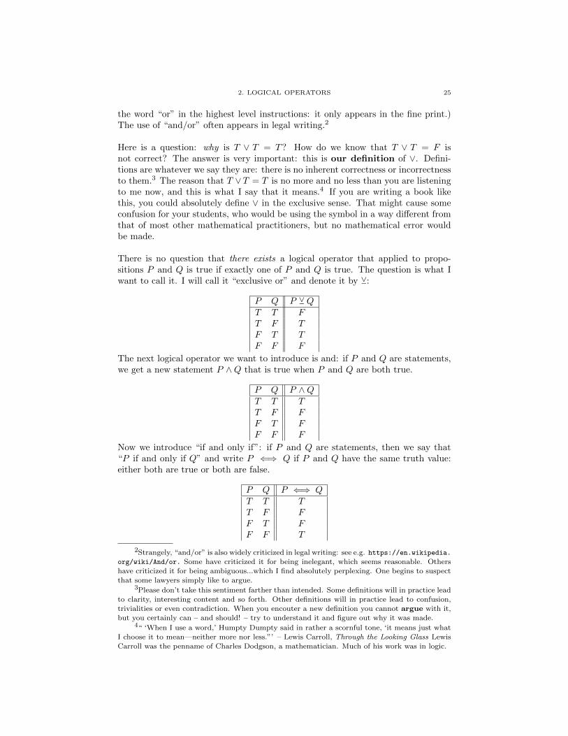
There is no question that there exists a logical operator that applied to propo-sitions P and Q is true if exactly one of P and Q is true. The question is what Iwant to call it. I will call it “exclusive or” and denote it by Y:

P Q P YQT T FT F TF T TF F F

The next logical operator we want to introduce is and: if P and Q are statements,we get a new statement P ∧Q that is true when P and Q are both true.

P Q P ∧QT T TT F FF T FF F F

Now we introduce “if and only if”: if P and Q are statements, then we say that“P if and only if Q” and write P ⇐⇒ Q if P and Q have the same truth value:either both are true or both are false.

P Q P ⇐⇒ QT T TT F FF T FF F T

2Strangely, “and/or” is also widely criticized in legal writing: see e.g. https://en.wikipedia.

org/wiki/And/or. Some have criticized it for being inelegant, which seems reasonable. Othershave criticized it for being ambiguous...which I find absolutely perplexing. One begins to suspect

that some lawyers simply like to argue.3Please don’t take this sentiment farther than intended. Some definitions will in practice lead

to clarity, interesting content and so forth. Other definitions will in practice lead to confusion,

trivialities or even contradiction. When you encouter a new definition you cannot argue with it,but you certainly can – and should! – try to understand it and figure out why it was made.

4“ ‘When I use a word,’ Humpty Dumpty said in rather a scornful tone, ‘it means just whatI choose it to mean—neither more nor less.”’ – Lewis Carroll, Through the Looking Glass Lewis

Carroll was the penname of Charles Dodgson, a mathematician. Much of his work was in logic.

26 2. LOGIC

3. Logical Equivalence, Tautologies and Contradictions

Let P1, . . . , Pn be statements. We say that two expressions X and Y formed fromthese statements using logical operators are logically equivalent if for each of the2n possible combinations of truth values of P1, . . . , Pn, the two expressions havethe same truth value. We write this for now as X ↔ Y .5

Here are some simple first examples of logical equivalence.

Example 2.4. Let P and Q be statements. Then:

a) We have

P ↔ ¬(¬P ).

Indeed, P is true exactly when ¬P is false exactly when ¬(¬P ) is true.b) We have

(P ∧Q)↔ (Q ∧ P ) :

Eeach expression is true precisely when P and Q are both true.c) We have

(P ∨Q)↔ (Q ∨ P ) :

Each expression is true precisely when at least one of P and Q is true.

Two logical expressions that are equal are certainly logically equivalent. The con-verse is not true: ¬(¬P ) is a different expression from P , but they are logicallyequivalent. This example already shows that for many purposes logical equivalenceis actually a more useful concept than equality. Consider the two statements “Itis raining” and “It is not the case that it is not raining.” Technically speakingthey are different statements, but that just means they are expressed with differentwords. In all cases where we actually care about the information conveyed by thestatements, they are interchangeable.

In Exercise 2.1 you are asked to establish that ∧ and ∨ are commutative andassociative, up to logical equivalence.

Here is a very useful logical equivalence.

Proposition 2.5 (Logical DeMorgan’s Laws). Let P and Q be statements.

a) We have ¬(P ∨Q)↔ (¬P ) ∧ (¬Q).b) We have ¬(P ∧Q)↔ (¬P ) ∨ (¬Q).

Proof. These and similar logical equivalences can be verified in a straight-forward way: here, we actually write down all four possible combinations of thetruth/falsity of P and the truth/falsity of Q and check that in each of these fourcases, the first logical expression involving P and Q is true exactly when the secondlogical expression involving P and Q is true.a) The following truth table establishes ¬(P ∨Q)↔ (¬P ) ∧ (¬Q).

5Yes, this is very similar to the previously introduced notation X ⇐⇒ Y . This will beelaborated upon shortly.

4. IMPLICATION 27

P Q ¬(P ∨Q) (¬P ) ∧ (¬Q)T T F FT F F FF T F FF F T T

b) The following truth table establishes ¬(P ∧Q)↔ (¬P ) ∨ (¬Q).

P Q ¬(P ∧Q) (¬P ) ∨ (¬Q)T T F FT F T TF T T TF F T T

�

A tautology is a logical expression involving statements P1, . . . , Pn that is true forall 2n possible truth values of the individual statements Pi. A contradiction isa logical expression involving statements P1, . . . , Pn that is false for all 2n possibletruth values of the individual statements Pi.

Thus a logical expression X is a tautology precisely when its negation ¬X is acontradiction.

Example 2.6.a) The statement P ∨ (¬P ) is a tautology: exactly one of P and ¬P is true and thusP ∨ (¬P ) is always true.

b) The statement P ∧ (¬P ) is a contradiction: exactly one of P and ¬P is true andthus P ∧ (¬P ) is false.

c) Indeed, using Proposition 2.5 we find that

¬(P ∨ (¬P ))↔ (¬P ) ∧ (¬¬P )↔ (¬P ) ∧ P ↔ P ∧ (¬P ).

Thus the logical expression of P ∧ (¬P ) is logically equivalent to the negation of thetautology P ∨ (¬P ), so it is a contradiction.

Here is a simple but fundamental observation:

Proposition 2.7. Let X and Y be logical expressions involving statementsP1, . . . , Pn. Then X ↔ Y holds exactly when X ⇐⇒ Y is a tautology.

Proof. The assertion X ↔ Y means that for each of the 2n possible truthvalues of P1, . . . , Pn, the expression X is true exactly when the expression Y istrue. If so, then for each of the 2n possible truth values of P1, . . . , Pn, we haveX ⇐⇒ Y . Similarly, if X ⇐⇒ Y is a tautology then for each of the 2n possibletruth values of P1, . . . , Pn the expression X ⇐⇒ Y is true, which means that foreach of the 2n possible truth values of P1, . . . , Pn, the expression X is true exactlywhen the expression Y is true. �

4. Implication

We now come to the most important logical operator: implication. For statementsP and Q, write P =⇒ Q and say “P implies Q” for the operator defined as follows:

28 2. LOGIC

P Q P =⇒ QT T TT F FF T TF F T

As mentioned above, like Humpty Dumpty I can make any definition I want. Sothat’s what implication means because I say so. You can’t argue!

Well....you can’t argue, but you can still wonder why I made my definition oreven be confused about it. For many people, the last two lines of the defining truthtable are confusing: why is P =⇒ Q true whenever P is false?

One can think of the implication P =⇒ Q as working like a contract: if youdo P , I promise to do Q. How can such a contract be broken? To be more con-crete, suppose that P is that you have a completed Jittery Joe’s punch card andQ is that you get a free drink of your choosing at Jittery Joe’s. Then the wholebusiness is encapsulated in the contract P implies Q: if you turn in your punchcard, you get a free drink. What would constitute breaking this contract? The onlyway is that if you turn in the punchcard and they refuse to give you a free drink:T =⇒ F is precisely what shouldn’t happen. Can the contract become broken ifyou do not turn in your punch card? No, of course not. If you don’t turn in yourpunch card, you might still get a free drink6, and if you do that certainly doesn’tinvalidate the contract. What if you don’t turn in your punch card and don’t geta free drink? Of course that’s what’s happening at most points in your life: thatdoesn’t invalidate the contract either.

I find it useful to think of binary logical operators – i.e., expressions involvingP and Q defined by 4 row truth tables – in terms of the number of times thatthey are true...in the sense of the number of T’s that appear in the defining columnof the table. A tautology is defined by being true four our of four times, whilea contradiction is defined by being true zero out of four times. Knowing that anoperator is true one, two or three times out of four doesn’t determine the operatorup to logical equivalence, but it is still useful information. Like ∨, the operator=⇒ is true 3 out of 4 times.

Why is this useful? Well, for instance one of the mistakes that students at thislevel make again and again is thinking that ¬(P =⇒ Q) comes out again as somekind of implication. But the above reasoning shows that this is not possible. Sincean implication is true 3 out of 4 times, its implication is true 1 out of 4 times...henceis not an implication. In fact this reasoning puts us on the right track for a logicallyequivalent operator to ¬(P =⇒ Q): what other operators do we know that aretrue 1 out of 4 times? The one that springs to mind is ∧. This does not mean that¬(P =⇒ Q)↔ P ∧Q and in fact this isn’t true: since P ∧Q is true exactly whenP and Q are true, while ¬(P =⇒ Q) is true exactly when P =⇒ Q is false,which as just mentioned is exactly when P is true and Q is false. Aha!

6As someone who has spent countless hours in various Jittery Joe’s, I am here to tell youthat punch cardless free drinks happen every now and again.

4. IMPLICATION 29

Proposition 2.8. Let P and Q be statements.

a) We have ¬(P =⇒ Q)↔ P ∧ (¬Q).b) We have (P =⇒ Q)↔ (¬P ) ∨Q.

Proof. a) This was discussed above: ¬(P =⇒ Q) and P ∧ (¬Q) are eachtrue when P is true and Q is false and in none of the other 3 cases.b) Using Proposition 2.5 we get

P =⇒ Q↔ ¬(¬(P =⇒ Q)↔ ¬(P ∧ (¬Q))

↔ (¬P ) ∨ (¬¬Q)↔ (¬P ) ∨Q. �

Thus the two “three out of four” operators ∨ and =⇒ are not logically equiva-lent...but =⇒ is logically equivalent to an operator involving ∨.

Here are some more important logical equivalences involving implication.

Proposition 2.9. For statements P and Q, we have

P ⇐⇒ Q↔ (P =⇒ Q) ∧ (Q =⇒ P ).

Proof. Any assertion about logical equivalence of binary logical expressions,no matter how fancy-looking, can be established just by writing out the four-rowedtruth table. So here we go:

P Q P ⇐⇒ Q (P =⇒ Q) ∧ (Q =⇒ P )T T T TT F F FF T F FF F T T

�

One all-important consequence is that two statements are equivalent precisely wheneach implies the other. In practice, it is most often the case that to prove A ⇐⇒ Bwe prove A =⇒ B and then B =⇒ A.

We now introduce three variants on the implication P =⇒ Q:

1) The converse implication Q =⇒ P .2) The inverse implication (¬P ) =⇒ (¬Q).3) The contrapositive (¬Q) =⇒ (¬P ).

The key question is which of these variations on implication are logically equiv-alent and especially, whether any of them is logically equivalent to P =⇒ Q. Andagain, no problem to answer any question of this type: just make a truth table:

P Q P =⇒ Q Q =⇒ P (¬P ) =⇒ (¬Q) (¬Q) =⇒ (¬P )T T T T T TT F F T T FF T T F F TF F T T T T

Contemplation of the table establishes the following result.

30 2. LOGIC

Proposition 2.10. Let P and Q be statements.

a) The implication P =⇒ Q and the contrapositive (¬Q) =⇒ (¬P ) arelogically equivalent to each other.

b) The converse implication Q =⇒ P and the inverse implication (¬P ) =⇒(¬Q) are logically equivalent to each other.

c) The implication is not logically equivalent to either the converse implica-tion or to the inverse implication.

For students of mathematics, distinguishing between P =⇒ Q and Q =⇒ P isusually not a problem: all squares are rectangles, but not all rectangles are squares.OK! However, in everyday life confusion between these two assertions is so abun-dant that there is a name for it: the converse fallacy.

Proposition 2.10a) will later become the basis for an important proof technique,proof by contraposition.

5. The Logic of Contradiction

Proposition 2.11. For any statements P and Q, the following is a tautology:

((¬P ) =⇒ (Q ∧ ¬Q)) =⇒ P.

Proof. Of course we could establish this with a truth table. But instead, letus talk it out: like any implication, it is true unless its hypothesis is true and itsconclusion is false, so we must rule that out. Namely, we must rule out that both

(¬P ) =⇒ (Q ∧ ¬Q)

and

¬Phold. But if so, then Q ∧ ¬Q holds, which it doesn’t. �

In Proposition 2.11 we could replace (Q∧¬Q) with any logical contradiction: thatis, with any statement that evalues to false whether P itself is true or false. Howeverthe idea of Proposition 2.11 is that it models the most common form of a proof bycontradiction: you want to establish P , so for the sake of argument suppose that Pis false. If from this you can deduce two contradictory statements Q and ¬Q, thenyour argument has reached a false conclusion so you must have a false premise. Butyour only premise was that P was false, so it must be that P is true.

6. Logical Expressions Revisited

Let us think a bit more about logical expressions in the statements P1, . . . , Pn.What is such a thing?

If we construe syntactically different expressions as different, thn even using theexpressions we have already defined, there are clearly infinitely many different log-ical expressions involving even one statement P , e.g.

P, (P ∨ P ),¬¬P, (P ∧ P ∧ P )

and so forth. So it makes much more sense to consider logical expressions inP1, . . . , Pn only up to logical equivalence. How many such expressions are there,and can we describe them all?

6. LOGICAL EXPRESSIONS REVISITED 31

To define a logical expression up to logical equivalence really means filling in acolumn of a truth table with 2n rows – each row corresponding to one of the pos-sible combinations of the truth values of P1, . . . , Pn. Since we have 2n entries tofreely fill in with either T or F , it follows that there are precisely 22

n

inequivalentlogical expressions involving the statements P1, . . . , Pn.

Example 2.12. Let’s write down all the inequivalent logical expressions in the

statement P . There are 221

= 4 such expressions. We have seen them all already:they are P , ¬P , T – i.e., the tautology: always true – and F – i.e., the contradiction:always false.

We haven’t defined a “tautology symbol” or a “contradiction symbol” yet – dowe need to? No, as mentioned before we have

T ↔ P ∨ (¬P ), F ↔ P ∧ (¬P ).

So all of the inequivalent logical expressions in P are obtained from P , ∨, ∧ and ¬.

Example 2.13. Let’s write down all the inequivalent logical expressions in the

statements P and Q. There are 222

= 16 of them. Here they are.

a) T ↔ P ∨ (¬P ).b) P ∨Q.c) (P =⇒ Q)↔ (¬P ) ∨Q.d) (Q =⇒ P )↔ (¬Q) ∨ P .e) P =⇒ (¬Q)↔ (¬P ) ∨ (¬Q).f) P .g) ¬P .h) Q.i) ¬Q.j) P ⇐⇒ Q↔ (P ∧Q) ∨ (¬P ∧ ¬Q).k) P ⇐⇒ (¬Q)↔ (P ∧ ¬Q) ∨ (¬P ∧Q).l) P ∧Q.

m) (¬P ) ∧Q.n) P ∧ (¬Q).o) (¬P ) ∧ (¬Q).p) F ↔ P ∧ (¬P ).

How do we know all these expressions are inequivalent? All we have to do is writedown the truth tables – you are asked to do this in Exercise 2.3. When the mostfamiliar version of this expression is not built up out of P , Q, ¬, ∨ and ∧ we havegiven an equivalent expression that is built up in this way. This shows that thereare no “essentially new” logical expressions in P and Q: the ones we have alreadyintroduced can be combined to yield every logical expression (up to equivalence).

Example 2.14. There are 223

= 256 inequivalent logical expressions in thestatements P1, P2 and P3. We could list them all in a truth table with 23 = 8 rows

and 223

= 256 columns. Then we can, one by one, try to write these expressions interms of P1, P2, P3, ¬, ∨ and ∧. Do you want to do this? Me neither – let us tryto come up with a more general, conceptual approach.

Let P1, . . . , Pn be statements. For any list ` : a1, . . . , an of length n with entries in{T, F}, we can build a logical expression out of P1, . . . , Pn, ¬ and ∧ that is true

32 2. LOGIC

precisely when for all 1 ≤ i ≤ n the truth value of Pi is ai: for 1 ≤ i ≤ n let us put

P aii :=

{Pi if ai = T

¬Pi if ai = F.

Then the expression we have in mind is

(P a11 ) ∧ (P a22 ) ∧ . . . ∧ (P ann ).

For instance, if the list is ` : T, T, F, F, T then the expression is

X` : P1 ∧ P2 ∧ (¬P3) ∧ (¬P4) ∧ P5.

This expression evaluates to true if and only if the truth value of Pi is ai for all i, soit does what we want. This corresponds to a logical expression whose correspondingcolumn in the truth table has a single T in the row corresponding to the list ` andhas all 2n − 1 other entries F.

As above, the contradiction F can be achieved as P1 ∧ (¬P1). Every other log-ical expression has some number 1 ≤ m ≤ 2n entries equal to T , and these entriescorrespond to certain lists `1, . . . , `m of length n with entries in {T, F}. Thereforethe logical expression that gives the correct column in the truth table is

X`1 ∨X`2 ∨ . . . ∨X`m .

We have shown the following result:

Proposition 2.15. Every logical expression in P1, . . . , Pn can (up to logicalequivalence) be built up out of P1, . . . , Pn, ¬, ∨ and ∧.

Could we go further? That is, do we need all of ¬, ∨ and ∧? Well, just by takingn = 1 we see that we need ¬, since P ∧P ↔ P ∨P ↔ P . On the other hand, giventhat we use ¬, we do not need both of ∨ and ∧: Proposition 2.5 tells us how toexpress either one of ∨, ∧ in terms of the other and ¬. Thus we get:

Proposition 2.16. a) Every logical expression in P1, . . . , Pn can (up tological equivalence) be built up out of P1, . . . , Pn, ¬ and ∨.

b) Every logical expression in P1, . . . , Pn can (up to logical equivalence) bebuilt up out of P1, . . . , Pn, ¬ and ∧.

Proposition 2.16 looks like the end of this road: using P1, . . . , Pn and ¬ it is clearthat we can build up exactly 2n logically inequivalent expressions:

P1, ¬P1, P2,¬P2, . . . , Pn,¬Pn.When n = 1 this gives us all 2n inequivalent expressions, but for n ≥ 2 it does not.However we can go further: I claim there is a binary logical operator X(P1, P2)such that using P1, P2 and X(P1, P2) one can build ¬ and ∧ and thus every logicalexpression. In fact, I claim that precisely 2 of the 16 binary logical operators inExample 2.13 have this property. You are asked to show this in Exercise 2.4.

Is Exercise 2.4 significant? Not to us, no...though it seems interesting. But there areconnections between logical expressions and electrical engineering: one can think ofan n-ary logical circuit (or “gate”) as something that takes n different wires as in-put and has 1 output wire. Depending upon which of the input wires carry current,the circuit decides whether the output wire carries current. Letting T correspondto “carries current” and F correspond to “does not carry current,” the possible

7. OPEN SENTENCES AND QUANTIFIERS 33

n-ary logical circuits correspond to the 22n

logical expressions in P1, . . . , Pn. Now22n

grows very rapidly: e.g. there are 65, 536 different 4-ary logical circuits. Itwould be ridiculous for someone to need 65, 536 different kinds of circuits on hand.Proposition 2.15 shows that we can get away with one unary circuit (a “not gate”that converts current into no current and vice versa) and two binary circuits corre-sponding to ∧ and ∨. Proposition 2.16 shows that we only need one of the ∧ andthe ∨. Finally, Exercise 2.4 shows that one in fact needs just one binary circuit outof which all other logical circuits can be built. In my experience this fact is indeedbetter known to electrical engineers and computer scientists than mathematicians.

7. Open Sentences and Quantifiers

Consider the following sentence:

P (x, y): We have y = x2.

The sentence P (x, y) is not a statement, because its truth value depends on whatx and y are, and they are unspecified. Suppose that we consider x and y rangingover the real numbers. Then, of course, there are some pairs (x, y) ∈ R2 for whichP is true and other pairs (x, y) ∈ R2 for which P (x, y) is false. Indeed the graphof the function f(x) = x2 is precisely

{(x, y) ∈ R2 | P (x, y) is true},

so it is a parabola in the Cartesian plane.

We say that P (x, y) is an open sentence. In general, an open sentence P is likea statement, but it contains variables x1, . . . , xn which we understand to rangeover certain nonempty sets S1, . . . , Sn. We sometimes speak of

∏ni=1 Si as the do-

main of the open sentence P . Thus for each element (x1, . . . , xn) ∈∏ni=1 Si we

can “plug it into P” and thereby get a statement P (x1, . . . , xn). The truth valueof P (x1, . . . , xn) may of course depend upon the choice of (x1, . . . , xn), and then asabove we can consider the truth locus of P , namely

T(P ) := {(x1, . . . , xn) ∈n∏i=1

Si | P (x1, . . . , xn) is true}.

Proposition 2.17. Let P = P (x) be an open sentence with variable x rangingover the nonempty set S. Then we have

T(¬P ) = S \ T(P ).

You are asked to prove Proposition 2.17 in Exercise 2.6.

Thus an open sentence is a bit more interesting than a statement: whereas a state-ment is either true or false, or an open sentence we get to ask for which values it istrue and for which values it is false. However, it is very useful to be able to “col-lapse” an open sentence into a statement, which we can do by asserting somethingabout its truth locus T(P ). There are two standard ways to do this.

Universal quantifier: We introduce a new symbol ∀ that we read as “for all.”

34 2. LOGIC

Suppose that P = P (x) is an open sentence involving a variable x that ranges overthe nonempty set S. Then

(3) ∀x ∈ S, P (x)

is a statement: in words, it is “For all elements x in S, we have that P (x) is true.”It is true if and only if P (x) is true for all x ∈ S, or equivalently if the truth locusT(P ) is all of S. We call ∀ the universal quantifier. This terminology is because(I think) we are viewing S as our universal set, so if the truth locus is S then thesentence is “universally true” – that is, it holds for all elements of the universal set.

Example 2.18. a) We start with the open sentence P (x) : x2 + 1 > 0,where x ranges over the real numbers. Applying the universal quantifierwe get the statement

∀x ∈ R, x2 + 1 > 0.

The quantified statement is true, since for any real number x we havex2 ≥ 0 and thus x2 + 1 ≥ 1 > 0.

b) We start with the open sentence Q(x) : x2 − 1 > 0, where x ranges overthe real numbers. Applying the universal quantifier we get the statement

∀x ∈ R, x2 − 1 > 0.

The quantified statement is false: in order to be true it would have tohold for all x ∈ R, but it is false e.g. for x = 0. More precisely, we have

T(Q) = {x ∈ R | x2 − 1 > 0} = (−∞,−1) ∪ (1,∞).

So the truth locus of Q is the union of two intervals on the real line. Thatlocus is not all of R, so the universally quantified sentence is false.

c) We start with the open sentence R(x) : x2 + 1 ≤ 0, where x ranges overthe real numbers. Applying the universal quantifier we get the statement

∀x ∈ R, x2 + 1 ≤ 0.

The quantified statement is false. Indeed, R(x) = ¬P (x), so since thesentence P (x) holds for all x ∈ R, the sentence Q(x) holds for no x ∈ R:its truth locus T(R) is ∅.

Existential quantifier: We introduce a new symbol ∃ that we read as “thereexists.” Suppose that P = P (x) is an open sentence involving a varaible x thatranges over the nonempty set S. Then

(4) ∃x ∈ S, P (x)

is a statement: in words, it is “There exists x in S such that P (x) is true.” (Noticethat in translating (3) to words we added “we have”: this was just for reasonsof English usage, as it it better not to start a phrase with a symbol. The words“we have” add nothing to the meaning. Similarly, in translating (4) to words weadded “such that”: this is necessary in order to get a grammatically correct Englishsentence, but it does not make any mathematical change.) It is true if and only ifP (x) is true for some (i.e., at least one) x ∈ S, or equivalently if the truth locusT(P ) is nonempty. We call ∃ the “existential quantifier” for reasons that seem moreclear: elements of T(P ) exist.

Example 2.19. We revisit Example 2.18 with ∃ in place of ∀.


a) Consider the statement

∃x ∈ R, x2 + 1 > 0.

This is true, and to verify that it is enough to find one real number xsuch that x2 + 1 > 0. Since 02 + 1 = 1 > 0, that suffices. Previously weestablished that ∀x ∈ R, x2 + 1 was true. Observe that this is a strongerstatement: if something is true for all x ∈ R it is most certainly truefor some x ∈ R. This observation is completely general: for any opensentence P (x) with x ranging over the nonempty7 set S, we have

(∀x ∈ S, P (x)) =⇒ (∃x ∈ S, P (x)).

b) Consider the statement

∃x ∈ R, x2 − 1 > 0.

Since 22− 1 = 3 > 0, indeed there is an x ∈ R such that x2− 1 > 0. Thusthe statement is true. This was not a surprise, since earlier we observedthat T(Q) = (−∞,−1) ∪ (1,∞). In particular T(Q) 6= ∅, which is all weneed to see that the existentially quanitified statement is true.

c) Consider the statement

∃x ∈ R, x2 + 1 ≤ 0.

This is false: since for all x ∈ R we have x2 + 1 > 0, for no x ∈ R dowe have x2 + 1 ≤ 0. Here we started with an open sentence P (x) thatwas universally true and passed to its negation ¬P (x), which is thereforeuniversally false: the truth set switches from the universal set to the emptyset. Symbolically:

(5) ∀x ∈ S, P (x) ⇐⇒ ¬(∃x ∈ S, ¬P (x)).

We record an equivalent version of this observation as Proposition 2.20a),coming up next.

Proposition 2.20. Let P (x) be an open sentence with a variable x rangingover the nonempty set S.

a) We have

¬(∀x ∈ S, P (x)) ⇐⇒ ∃x ∈ S, ¬P (x).

b) We have

¬(∃x ∈ S, P (x)) ⇐⇒ ∀x ∈ S, ¬P (x).

Proof. a) By Proposition 2.17 we have

T(¬P ) = S \ T(P ).

So ¬(∀x ∈ S, P (x)) holds if and only if T(P ) ( S if and only if T(¬P ) = S\T(P ) 6=∅ (a subset of a universal set is proper if and only if its complement is nonempty)if and only if ∃x ∈ S, ¬P (x).

Alternately, we may apply ¬ to both sides of (5).b) Since ∃x ∈ S, P (x) holds if and only if T(P ) 6= ∅, we have ¬(∃x ∈ S, P (x)) ifand only if T(P ) = ∅ if and only if T(¬P ) = S if and only if (∀x ∈ S, ¬P (x)). �

7We are actually using here that the set S is nonempty.

36 2. LOGIC

One might expect there to be other quantifiers besides ∃ and ∀, but I only know ofone that is in common use: when we write

∃! x ∈ S, P (x)

and say “There is a unique x ∈ S such that P (x) holds” to mean that the setT(P ) of x ∈ S such that P (x) holds has exactly one element. (In general, theword “unique” is used in mathematics to mean that there is at most one.) It issomewhat tempting to invent new quantifiers, for instance ∃∞ could mean “Thereare infinitely many.” However it turns out that one can do quite well enough withthe old standbys of ∀ and ∃ (and occasionally ∃!). I will let you reflect on why thismight be the case.

We introduced open sentences as having several variables, but our discussion ofquantifiers has thus far been with sentences involving only one variable. In general,if you have an open sentence P (x1, . . . , xn) in which xi ranges over Si for 1 ≤ i ≤ n,one can apply either ∀, ∃ or neither one to each variable separately. In order toget a statement we should apply either quantifier to all of the variables; if we onlyquantify some of the variables then we are left with an open sentence whose domainis the Cartesian product of the unquantified variables. In logic one often speaks ofa variable as being bound by a quantifier and as unbound or free if no quantifieris applied. This terminology will be (only) occasionally helpful to us.

Example 2.21. One can think of ∃ as inducing a projection on the truth set.We illustrate this with two examples.

a) Consider the open sentence

P (x, y) : x = y2

with domain (x, y) ∈ R × R. Its truth locus is the horizontally openingparabola. Now consider

Q(x) : ∃x (x = y2),

with domain x ∈ R. For x ∈ R, Q(x) is true if and only if x is the squareof some other real number y, which holds if and only if x ≥ 0. Thus thetruth locus of Q is [0,∞). But now notice that if we project the parabola{(x, y) ∈ R2 | x = y2} onto the x-axis we get T(Q) = [0,∞).

b) Consider the sentence

P (x, y) :x2

4+y2

9= 1

with domain (x, y) ∈ R × R. Its truth locus is an ellipse centered at theorigin. The truth locus of

Q(x) : ∃y (x2

4+y2

9= 1)

is the set of x ∈ R such that 9(1 − x2

4 ) has a real square root, which

happens if and only if 1 − x2

4 ≥ 0, which happens if and only if |x| ≤ 2,so T(Q) = [−2, 2]. This is the projection of the ellipse onto the x-axis.Similarly for

R(y) : ∃x (x2

4+y2

9= 1)


the truth locus of R(y) is the set of y ∈ R such that 4(1 − y2

9 ) has a realsquare root, which happens if and only if |y| ≤ 3, so T(R) = [−3, 3]. Thisis the projection of the ellipse onto the y-axis.

Example 2.22. We consider various quantifications of the open sentence

P (x, y) : y > x

with domain (x, y) ∈ R× R.

a) If we don’t quanitify at all, then T(P ) is the set of points in the planelying over the 45 degree line y = x.

b) Consider

Q(x) : ∀y ∈ R, y > x.

Here we have written Q(x) because the variable y is bound by the quantifiery and therefore “used up”: we can’t plug in values for y. However, we canstill plug in values for x and thus we get an open sentence with domainx ∈ R. If we plug in x ∈ R, the statement Q(x) asserts that x is less thanevery real number. This is false no matter what x is, so T(Q) = ∅.

c) Consider

R(x) : ∃y ∈ R, y > x.

Again we get an open sentence with domain x ∈ R. If we plug in x ∈ R,the statement Q(x) asserts that some real number is greater than x. Thisis true no matter what x is: we can take y = x+ 1. So T(R) = R.

d) Consider the statement

∀x ∈ R, ∃y ∈ R y > x.

This statement asserts that R(x) is true for all x ∈ R, which as we sawabove is true, so the statement is true.

e) The statement

∀x ∈ R,∀y ∈ R, y > x

asserts that every real number is greater than every other real number.This is false.

f) The statement

∃x ∈ R,∃y ∈ R, y > x

asserts that there are real numbers x and y such that y > x. This is true:1 > 0.

g) Consider the statement

∃x ∈ R, ∀y ∈ R, y > x.

This statement asserts that there is a real number x that is smaller thanevery real number. This is false.

Now for a very important observation: the statements

∀x ∈ R, ∃y ∈ R y > x

and

∃x ∈ R, ∀y ∈ R, y > x

are identical except for the order of the quantifiers: the first one has ∀ then ∃,whereas the second has ∃ then ∀. The first statement is true and the second state-ment is false. Thefore changing the order of the quantifiers can change the

38 2. LOGIC

meaning and truth value of a statement. More precisely, swapping ∃ and ∀can change the meaning of a statement: in fact it usually does in a dramatic way.Moving two existential quantifiers past each other does not change the meaning oftruth value of a statement (or the meaning or truth locus of an open sentence):∃x1 ∈ S1, ∃x2 ∈ S2 means “There is x1 in S1 and x2 in S2 such that...” whichmeans the same thing as “there is x2 ∈ S2 and x1 ∈ S2 such that...”

Often it is a reasonable perspective to count repeated instances of the same quan-tifier as one single quantifier: this is because e.g.

∀x1 ∈ S1,∀x2 ∈ S2

means the same thing as∀(x1, x2) ∈ S1 × S2.

On the other hand, the more “alternating quantifiers” a statement has, the morecomplex it is both logically and mathematically. A statement with a single quan-tifier is usually immediately understood. Statements with two quantifiers oftenrequire a little thought. Statements with at least three quantifiers often requirespecial training to properly understand.

Example 2.23. Let f : R→ R be a function. The definitions of “limx→c f(x)”and “f is continuous at c” involve three quantifiers. It is probably because of theirlogical complexity that they are not introduced in freshman calculus. For instance,here is the definition of continuity at 0: the function f is continuous at x = 0 if:

∀ε > 0 ∃δ > 0 ∀x ∈ R, |x| < δ =⇒ |f(x)− f(c)| < ε.

A note on uses of quantifiers: throughout much of mathematics, explicit use ofthe symbols ∀ and ∃ is not much encountered in formal mathematical writing: itis often preferable to use the words “for all” and “there exists” (or even “thereis”) instead. These symbols are more commonly encountered on the blackboard,in handwritten notes, and other less formal mathematical presentations. On theother hand there is a branch of mathematics, mathematical logic in which logicand its interactions with other parts of mathematics are studied (many of theseinteractions are more interesting and less “foundational” or “philosophical” thanone might expect), and in this part of mathematics the symbols ∃ and ∀ abound.

Perhaps because undergraduate “foundations” courses such as this one are afairly recent invention, mathematicians also differ among each other in how explicitthey are in their quantification. All mathematicians make use of quantifiers, butsome mathematicians prefer to leave certain quantifications explicit. As the previ-ous sentence suggests, I am not one of those mathematicians, and I think explicituse of quantifiers is a key part of accurate mathematical communication. But youshould be aware that “implied quantification” exists. When this happens, it is usu-ally the case that the implied quantifier is ∀, not ∃. This creates problems for somestudents, who when in doubt may supply the missing quantifier as ∃ because afterall that is a weaker assertion and therefore easier to prove.

Example 2.24. Horace is asked to prove: “A non-negative real number hasa real square root.” His answer: “The real number 9 is non-negative, and since32 = 9, we have that 3 is a real square root of 9.” Do you see the issue?

Horace has interpreted the statement as “There exists a non-negative real num-ber that has a real square root.” Outside of the context of mathematical discourse,

8. NEGATING STATEMENTS 39

one could defend his decision: after all the sentence begins with “A”. Perhaps Ho-race, as a student, is used to thinking of mathematical assertions as problems thatare being posed to him rather than logical statements that are either true or false.If one tacked the word “Find” onto the beginning of the sentence,we would not havea statement to prove but a command to follow, and what Horace wrote correctlyfollows that command.

But any mathematician would hear the unspoken universal quantifier and in-terpret the statement as “For all real numbers a ≥ 0, there is b ∈ R such thatb2 = a.” This is a much deeper assertion. It can be solved using the IntermediateValue Theorem from calculus (a result which, by the way, is not usually proved untila more advanced course) as follows: let a ≥ 0. If a = 0 then 0 is a real square rootof a, so we may assume a > 0. Now consider the function f : R→ R defined by

f(x) = x2 − a.We have f(0) = −a < 0. We also have

f(a+ 1) = (a+ 1)2 − a = a2 + a+ 1 > a2 − 2a+ 1 = (a− 1)2 ≥ 0.

Since f is a continuous function, f(0) < 0 and f(a+1) > 0, the Intermediate ValueTheorem implies that there is b ∈ R with 0 < b < a+ 1 such that

0 = f(b) = b2 − a.This means that b2 = a, so b is a square root of a.

In mathematics we usually want to prove “general statements” and not “examples.”So in the vast majority of mathematical results, we have a universally quantifiedstatement. In fact the most common form of a mathematical theorem is:

∀x ∈ S, P (x) =⇒ Q(x)

where P and Q are both open sentences with domain x. (The sentences P and Qmay themselves involve other quantifiers and often do.)

8. Negating Statements

In this section we have the relatively modest goal of giving some tips and practiceon negating statements.

Let us begin here: why would we want to negate statements? How does thiscome up in practice?

It is often said that the main goal in pure mathematics is to prove theorems. Thisis approximately true. But it omits something important: since we (not exclusively,but especially and most excitingly) want to prove new theorems, and a proof of atheorem is how we know the theorem is true, a somewhat more accurate statementof mathematical practice is that we have statements that we are very interestedin either proving or disproving statements. How does one go about disproving astatement P?

I can think of two good ways to do this.

First Method: Prove ¬P .

40 2. LOGIC

This works of course, since P is false if and only if ¬P is true. Construed thisway, the task of disproving has no formal difference from the task of proving: we’rejust trying to prove a different statement.

Second Method: Assume that P is true and deduce a logical contradiction.

This works too, of course, since if it cannot be the case that P is true, then itmust be that P is false.

Of these, the first method involves negating P . The second ostensibly does not.

Example 2.25. a) The Pythagorean school famously disproved that√

2is a rational number. The proof, which is perhaps the most famous of allmathematical proofs, will be given in full later, but it really does begin byassuming that

√2 is a rational number, writing

√2 = a

b for integers a andb with b 6= 0, and deducing a contradiction. There is no negation here (atleast, not yet).

b) Goldbach’s Conjecture states that every even integer n ≥ 4 is the sum oftwo prime numbers. It is widely believed to be true and known to hold forall 4 ≤ n ≤ 4 · 1018, but it is not currently proved. How could we dis-prove Goldbach’s Conjecture? My first point is that the idea of disprovingGoldbach’s Conjecture by contradiction seems ridiculous: we assume thatevery even integer n ≥ 4 is the sum of two primes and then try to reacha contradiction? How in the world are we going to do that?

In this case the only plausible way of disproving Goldbach’s conjectureis to prove its negative. Goldbach’s conjecture is that for all even n ≥ 4,there are prime numbers p1 and p2 such that n = p1 + p2. So its negationis: there exists an even n ≥ 4 such that for all prime numbers p1 and p2,we have n 6= p1 + p2. If this (the negation) is true and I give you the n,it is easy to check: for all prime numbers p < n you compute that n − pis not prime.

Negating statements also comes up when we are trying to prove P , not just disproveit. Most mathematical theorems have the form:

∀x ∈ S, P (x) =⇒ Q(x).

There are three basic ways of doing this:

I. Direct Proof: Let x ∈ S. (What follows either must work for all x ∈ S atthe same time or be divided into cases. We will discuss this in much more detaillater.) Assume that P (x) is true, and deduce that Q(x) is true.

II. Proof by Contrapositive: Let x ∈ S. (Same parenthetical comment asabove). Assume that ¬Q(x) is true and deduce that ¬P (x) is true.

III. Proof by Contradiction: Let x ∈ S. (Same parenthetical....) Assumethat P (x) is true and that ¬Q(x) is true and deduce a contradiction.

Two out of the three methods involve negating statements. Taken together, that ispretty good motivation!

8. NEGATING STATEMENTS 41

Next issue: isn’t the process of negation pretty trivial? Here, I will negate anarbitrary statement P :

¬P.In words, for any statement P its negation is “It is not the case that P holds.”

However, although this negation just by tacking “It is not the case that...” onthe front of a statement is logically valid, it is practically not very useful. Thepoint is that mathematical reasoning is all about deduction. We can build onsomething that is the case; it is much harder to build directly on what is not thecase. Here is a first example:

Proposition 2.26. For all x ∈ Z, if x2 is even, then x is even.

Proof. We will use the contrapositive: for x ∈ Z, if x is not even, then x2 is noteven. Okay, but what does it mean not to be even? In pre-university mathematicsone often defines an even number to be a whole number that is twice another wholenumber and an odd number to be a whole number that is not even...but this is notdirectly helpful. How do we build on the fact that x cannot be written as 2n forsome n ∈ Z? The key to moving on is to find an equivalent “positive” statement.As mentioned in Example 1.21 (and as we will prove later on), it turns out that ifan integer x is not even then it is of the form 2n + 1 for some n ∈ Z. This finallyis telling us something about x, and we can use it: if x = 2n+ 1 then

x2 = (2n+ 1)2 = 4n2 + 4n+ 1 = 2(2n2 + 2n) + 1

is also odd, completing the proof. �

That an integer that is not even is od the form 2n + 1 is an excellent example ofa “good negation.” The best (most useful) kind of negation doesn’t have the word“not” in it at all: instead of asserting the absence of something it is asserts thepresence of some other, complementary property. Exactly how this works dependson the particular example, but at a formal level our goal is to “work the negationfrom the outside in”: you will know that you’ve negated a logical expression in agood way when the negations just get applied to basic propositions, not to morecomplicated expressions.

Example 2.27. Some Good Negations:

a) A good negation of P =⇒ Q is P ∧ (¬Q). (This is as far as we can goin so much generality, but in practice you are left with the task of findinga good negation of Q.)

This example also comes with a warning: the negation of an im-plication is NOT an implication of any kind. In my experience,many students know this in pleasant circumstances but upon being suf-ficiently pressured (e.g. in an exam setting) will write something like“¬(P =⇒ Q) ↔ (¬P ) =⇒ (¬Q).” This is terribly wrong. I hopethat a “quantitative” approach helps here: as I stresed above, any impli-cation is a “3/4 operator”: one that is true for 3 out of 4 of the possiblecombinations of the basic truth values. Its negation therefore must be a“1/4 operator,” which is not a negation at all.

42 2. LOGIC

b) A good negation of P1 ∧ P2 ∧ P3 ∧ P4 is

(¬P1) ∨ (¬P2) ∨ (¬P3) ∨ (¬P4).

A good negation of Q1 ∨Q2 ∨Q3 is

(¬Q1) ∧ (¬Q2) ∧ (¬Q3).

These are logical DeMorgan’s Laws.c) A good negation of ∀x ∈ S, P (x) is

∃x ∈ S, ¬P (x).

A good negation of ∃x ∈ S, P (x) is

∀x ∈ S, ¬P (x).

Again, this shows that we want to work our negations “from the outsideto the inside.”

We now move on to some practical examples.

Example 2.28. We negate the statement “If I’m lying, I’m dying.’This statement has the form P =⇒ Q where P is “I’m lying” and Q is “I’mdying.” Following the template of Example 2.27a), a good negation would be:

I’m lying and I’m not dying.

It might be even better to express “I’m not dying” in a positive way, but I don’tknow a simple English construction that expresses this meaning exactly.

Example 2.29. We negate the statement “For every real number x there is alarger real number y.” More symbolically this is

∀x ∈ R ∃y ∈ R, y > x.

Let’s negate it from the outside in:

¬(∀x ∈ R ∃y ∈ R, y > x)

↔ ∃x ∈ R(¬(∃y ∈ R, y > x))

↔ ∃x ∈ R(∀y ∈ R,¬(y > x))

↔ ∃x ∈ R∀y ∈ R, y ≤ x.Thus the negated statement asserts that there is a largest real number, which meansthat the original statement could have been more pithily expressed as “There is nolargest real number.”

Example 2.30. We negate the following sentence8: “You can fool some of thepeople all of the time and all of the people some of the time, but you cannot fool allof the people all of the time.”

First we have to realize that the “but” is playing the logical role of an “and” sothe statement has the form A ∧B ∧ C with

A : You can fool some of the people all of the time.

B : You can fool all of the people some of the time.

C : You cannot fool all of the people all of the time.

8This sentence is traditionally attributed to Abraham Lincoln, but it does not seem clearwhether he actually said it.

9. EXERCISES 43

So the negation is ¬(A ∧B ∧C)↔ (¬A) ∨ (¬B) ∨ (¬C). Now we have to work onA, B and C individually, which are all themselves quantified statements.

Statement A takes the form: “For all times, there exists a person you can fool,”or more schematically “∀t ∃P such that you can fool P .” So its negation is: thereexists a time at which you can’t fool anyone.

Statement B takes the form “There exists a time such that you can fool all thepeople,” or more schematically “∃t ∀P you can fool P .” So its negation is: At alltimes, there is at least one person you can’t fool.

Happily, C has the form of a “cheaply negated” statement: “It is not the casethat you can fool all of the people all of the time.” So its negation is “At all times,you can fool all of the people.” Final answer:

At least one of the following holds: (i) There is at least one time where youcan’t fool anyone, or (ii) At all times there is someone you can’t fool, or (iii) At alltimes, you can fool everyone.

9. Exercises

Exercise 2.1. Let P , Q and R be statements.

a) Show: (P ∨Q)↔ (Q ∨ P ).b) Show: (P ∧Q)↔ (Q ∧ P ).c) Show: (P ∧Q) ∧R↔ P ∧ (Q ∧R).d) Show: (P ∨Q) ∨R↔ P ∨ (Q ∨R).

In light of parts c) and d) we usually write P ∧Q∧R in place of either (P ∧Q)∧R)or P ∧ (Q ∧R) and P ∨Q ∨R in place of either (P ∨Q) ∨R or P ∨ (Q ∨R).

Exercise 2.2. (Logical Distributive Laws) Let P , Q and R be statements.

a) Show: P ∨ (Q ∧R)↔ (P ∨Q) ∧ (P ∨R).b) Show: P ∧ (Q ∨R)↔ (P ∧Q) ∨ (P ∧R).

Exercise 2.3. Write down a truth table with 4 rows and 16 columns thatverifies that the 16 logical expressions written down in Example 2.13 are all logicallyinequivalent.

Exercise 2.4. Let P1 and P2 be statements.

a) Show that there is a logical expression X(P1, P2) such that using P1, P2

and X(P1, P2 one can build both ¬ and ∧. Hence all 22n

n-ary logicalexpressions can be built up out of P1, . . . , Pn and the expression X(P1, P2).(Hint: in fact we will have X(P1, P1) = ¬P1.)

b) Show that precisely 2 out of the 16 binary logical expressions have thisproperty.

Exercise 2.5. Prove the following tautology:9 For statements P and Q,

(P ∧ (P =⇒ Q)) =⇒ Q.

Exercise 2.6. Prove Proposition 2.17.

Exercise 2.7. How is Proposition 2.20 related to DeMorgan’s Laws? Discuss.

9It is called modus ponens. This name is not however much used by those in mathematicsbut rather in other academic subjects in which logic arises, like philosophy.

CHAPTER 3

Counting Finite Sets

1. Cardinality of a Finite Union

The basic problem we are interested in is the following: suppose we have finitesets A1, . . . , AN , and let

A :=

N⋃i=1

Ai

be their union. Suppose that we know the sizes #A1, . . .#AN of these sets. Canwe determine the size of A?

No, we cannot. Suppose A1 is the set of people in Athens, GA who own a carand A2 is the set of people in Athens, GA who own a cell-phone, so A is the set ofpeople in Athens, GA who own a car or a cell-phone (or both). If #A1 = n1 and#A2 = n2, then what we can say is that

max(n1, n2) ≤ #A ≤ n1 + n2.

Here, for real numbers x and y, max(x, y) denotes the larger of x and y.

The first inequality is pretty clear: a subset of a finite set has size at most that of theset itself (Exercise 1.4), which shows that n1 ≤ #A and n2 ≤ #A; since max(n1, n2)is equal to n1 or n2 (or both, if n1 = n2) it follows that max(n1, n2) ≤ #A. Asfor the inequality #A ≤ n1 + n2, it can be seen as follows: if we make a list ofeveryone who has a car in Athens and then we make a list of everyone who has acell-phone in Athens, and then tape the second list to the bottom of the first list,then we get a list whose associated set is A. However, #A could be smaller thann1 +n2, because even assuming that the first two lists were irredundant so that thefirst list `1 has size n1 and the second list `2 has size n2, the new list, say ` thatwe get by putting `1 and `2 together may be redundant, which by Exercise 1.2 iswhat would cause the associated set A to have cardinality less than the length of `.1

This motivates us to establish several things in more generality and with morecare, as we now do. First of all, if `1 and `2 are finite lists, it does make perfectsense to “combine them” into another finite list. This could be done in severaldifferent ways, but the way we just alluded to is perfectly good: if we have lists

`1 : x1, . . . , xm

of length m and`2 : y1, . . . , yn

1In this case we certainly do have #A < n1 +n2: not to brag too much, but I live in Athensand I have both a car and a cell-phone.

45

46 3. COUNTING FINITE SETS

of length n, we define the concatenated list

`1 + `2 : x1, . . . , xm, y1, . . . , yn,

of length m + n. For that matter we can do the same with any finite number offinite lists `1, . . . , `N . This allows us to establish the following:

Theorem 3.1 (Sum Theorem).

Let A1, . . . , AN be finite sets, and put A :=⋃Ni=1Ai. Then:

a) We have

max(#A1, . . . ,#AN ) ≤ #A ≤ #A1 + . . .+ #AN .

b) We have that #A = #A1 + . . .+ #AN if and only if the sets are pairwisedisjoint: for all 1 ≤ i 6= j ≤ N we have Ai ∩Aj = ∅.

Proof. a) Let 1 ≤ i ≤ N . Then Ai ⊆ A, so by Exercise 1.4 we have #Ai ≤#A. Again max(#A1, . . . ,#AN ) = #Ai for some 1 ≤ i ≤ N , so we have

max(#A1, . . . ,#AN ) ≤ #A.

Now for 1 ≤ i ≤ N , let ì be an irredundant finite list with associated set Ai, so byExercise 1.2 the list ì has length #Ai. Now form the list

` := `1 + . . .+ `N ,

it has length #A1 + . . . + #AN and associated set A since every element of Aappears on at least one of the lists, and conversely every entry in each list is anelement of A. By Exercise 1.3 this shows that #A ≤ #A1 + . . .+ #AN , completingthe proof of part a).b) Exercise 1.2 shows that #A is equal to the length of the list ` if and only ifthe list ` is irredundant. Since ` was contained by concatenating irredundant lists`1,. . . ,`N , a repetition in ` occurs if and only if there are 1 ≤ i 6= j ≤ N such thatsome entry on the list ì is equal to some entry on the list `j , which happens if andonly if Ai ∩Aj 6= ∅. �

Despite the somewhat heavy notation and pedantic proof, the ideas behind Theo-rem 3.1 are very simple and familiar. The result says that if we partition a finiteset into parts, then the size of the set is equal to the sum of the sizes of the parts:okay! On the other hand, if we express a finite set as a union of overlapping subsets,then the sum of the sizes of the subsets will be an overestimate on the size of theset...because elements in overlapping sets get counted at least twice.

Indeed, overlap is a key word here. In the motivating example, the extra pieceof information we need is the number of Athenians who have both a car and acell-phone: this number should be subtracted off from #A1 + #A2 (the number ofpeople who have a car plus the number of people who have a cell-phone). So:

Proposition 3.2. Let A1 and A2 be finite sets, and put A := A1 ∪A2. Then:

#A = #A1 + #A2 −#(A1 ∩A2).

Proof. Let us give two proofs.First Proof: Let’s go back to our construction with lists: let `1 be an irredundantfinite list with associated set A1, let `2 be a finite list without repeittions withassociated set A2, and let ` := `1 + `2. What we said so far is that ` is a finitelist, of length #A1 + #A2 with associated set A, but if A1 ∩ A2 6= ∅ then it is

1. CARDINALITY OF A FINITE UNION 47

redundant. There is just one new thing to say: the number of repetitions in ` is#A1 ∩ A2. More precisely, each element x ∈ A1 ∩ A2 appears (exactly once) ineach of `1 and `2; if we remove the second occurrence of each such element x, thenwe have removed #(A1 ∩ A2) elements to get a list `′ with no repeated elementsand still with associated set A. Thus the size of A is the length of `′, which is thelength of ` minus #(A1 ∩A2), which is #A1 + #A2 −#(A1 ∩A2).Second Proof: We define subsets

B1 := A1 \A2,

B2 := A1 ∩A2,

B3 := A2 \A1.

As we can see immediately from a Venn diagram, we have

A = B1

∐B2

∐B3,

so Theorem 3.1 gives

#A = #B1 + #B2 + #B3.

A Venn diagram also easily shows us that

A1 = B1

∐B2 and A2 = B2

∐B3,

so applying Theorem 3.1 once again, we get

#A1 + #A2 −#(A1 ∩A2) = (#B1 + #B2) + (#B2 + #B3)−#B2

= #B1 + #B2 + #B3 = #A. �

Let’s look for an analogue of Proposition 3.2 when we have three finite sets A1, A2

and A3 and A = A1 ∪A2 ∪A3. Again the interesting case is when the sets A1, A2,A3 are not pairwise disjoint; in this case Theorem 3.1 tells us that

#A < #A1 + #A2 + #A3,

but now “overlap” has become more complicated: presumably it should involvesome or all of

A1 ∩A2, A1 ∩A3, A2 ∩A3, A1 ∩A2 ∩A3.

If we guessed that “pairwise overlap was enough” we might try showing that #Ais equal to

(6) #A1 + #A2 + #A3 −#(A1 ∩A2)−#(A1 ∩A3)−#(A2 ∩A3).

However in the case that A = A1 = A2 = A3 the above formula evaluates to 0 ratherthan #A. This may suggest that just as #A1 + #A2 + #A3 is an overestimatefor #A and needs to be corrected by subtracting pairwise intersections, then (6) isan (albeit better) underestimate for #A and needs to be corrected by adding thetriple intersection. This turns out to be true:

Proposition 3.3. Let A1, A2, A3 be finite sets; put A := A1 ∪A2 ∪A3. Then:(7)#A = #A1+#A2+#A3−#(A1∩A2)−#(A1∩A3)−#(A2∩A3)+#(A1∩A2∩A3).


One way to prove Proposition 3.3 is to use Venn diagrams as above: we breakA1 ∪ A2 ∪ A3 into the 23 − 1 = 7 “elementary regions” that comprise the Venndiagram, one of which is A1 ∩A2 ∩A3. Breaking A1, A2, A3, A1 ∩A2, A1 ∩A3 andA2 ∩A3 into unions of elementary regions, one arrives a slightly tedious but totallydoable calculation, which the reader is asked to do in Exercise 3.1.

This is however neither the most enlightening approach nor the one that is mostamenable to general N , in which one would have to deal with a Venn diagram with2N −1 regions. Here is a different approach. The basic idea is to focus on how eachelement x ∈ A contributes to the right hand side of (7). If you ask me to state thatformally, I will respond that we want to check that for all x ∈ A, we have

1 = #(A1 ∩ {x}) + #(A2 ∩ {x}) + #(A3 ∩ {x})

−#(A1∩A2∩{x})−#(A1∩A3∩{x})−#(A2∩A3∩{x})+#(A1∩A2∩A3∩{x}),

for then summing that over all x ∈ A gives (7). But after seeing the argument youmight want to think about how it makes the most sense to you.

Case 1: Suppose that x lies in exactly one of A1, A2, A3, hence in none of thesets A1 ∩ A2, A1 ∩ A3, A2 ∩ A3 or A1 ∩ A2 ∩ A3, so it contributes 1 to the righthand side of (7).

Case 2: Suppose that x lies in exactly 2 of A1, A2, A3, hence in exactly one ofA1∩A2, A1∩A3, A2∩A3 and does not lie in A1∩A2∩A3. Therefore x contributes1 + 1− 1 = 1 to the right hand side of (7).

Case 3: Suppose that x lies in all of A1, A2, A3 and hence also in all of A1∩A2,A1∩A3, A2∩A3 and A1∩A2∩A3. Then overall x contributes 1+1+1−1−1+1 = 1to the right hand side of (7).

2. Independent Choices and Cartesian Products

How many cards are in a standard deck of playing cards? 52. Why?

That’s a bit of a strange question, but we can answer it in terms of some otherfamiliar facts:

• Every card has exactly one of four suits: clubs, diamonds, hearts or spades.• Every card has exactly one of thirteen values: two, three, four, five, six, seven,eight, nine, ten, jack, queen, king, or ace.• Every possible combination of suit and value occurs exactly once.

Given this, the answer is that 4 · 13 = 52.

This is an example of the Principle of Independent Choices. Suppose thatwe have two choices to make. For each choice, there are finitely many options:say that we have n1 ∈ Z+ options for the first choice and n2 ∈ Z+ options for thesecond choice. Suppose also that the choices are independent in the sense that what-ever we choose among the first set of options does not restrict our choice among thesecond set of options. Then the total number of ways to make these choices is n1 ·n2.

We can state a result with any finite number N ∈ Z+ of choices instead of two:

2. INDEPENDENT CHOICES AND CARTESIAN PRODUCTS 49

Proposition 3.4 (Principle of Independent Choices). Let N ∈ Z+. Supposethat we have N choices to make. For 1 ≤ i ≤ N , suppose that we have ni ∈ Z+

options for the ith choice. Suppose further that the choices are independent, in thesense that all combinations of choices among different options are possible. Thenthe total number of ways to make these N choices is n1 · · ·nN .

What do we think about Proposition 3.4? Is it obvious? Does it require proof?

My answers are “yes” and “yes, if possible.” Notice that in the proof of Proposition1.20 we already used the Principle of Indpendent Choices to argue that a set withN elements has 2N subsets: we observed that forming a subset of {x1, . . . , xN}amounts to successively choosing to include or exclude xi for 1 ≤ i ≤ N ; this givesN independent choices with two options each, hence by Proposition 3.4 there are2N options all together.

But in theoretical mathematics everything must be proved in terms of some setof assumptions, including basic ones called axioms. Although we do not needto have the basic axioms in full view at all (or even most) times, nevertheless inprinciple there should be a fixed set of axioms: we don’t add to our list of axiomseverytime something sounds obvious and we don’t know how to prove it. Thiswould turn mathematics into some kind of second-rate comic book, where the heroresolves their latest scrape by means of a superpower that has never been mentionedbefore that issue.

In this course we do not consider formal axioms for sets, but rather manipulatethem in intuitively plausible ways (that can, and have, been justified by formalaxioms). We also do not construct any of the basic number systems or the basicoperations on them, and therefore some properties of numbers will not be provableby us because the proofs are too closely bound to the constructions of these sys-tems. Are we in one of these cases now?

Sort of. To clarify what is going on, we observe that Proposition 3.4 is equiva-lent to the following result.

Proposition 3.5 (Cardinality of Finite Cartesian Products). Let N ∈ Z+,and let A1, . . . , AN be finite sets. Then

#(A1 × . . . AN ) = (#A1)× . . . (#AN ).

To see the relationship between Propositions 3.4 and 3.5, we observe that in thesetting of Proposition 3.4 we can let A1 be the set of options for the first choice, A2

be the set of options for the second choice, and so forth, finally letting AN be theset of options for the Nth choice. Then a collection of independent choices fromthese sets is precisely a finite list of length N ,

` : c1, . . . , cN

with ci ∈ Ai. As above, just by adding parentheses: c1, . . . , cN 7→ (c1, . . . , cN ), suchlists may be identified with elements of the Cartesian product A1× . . .×AN . Thisshows that Proposition 3.5 implies Proposition 3.4, and the converse implication is


almost the same.2

Let us now concentrate on Proposition 3.5 instead, since it is formulated in termsof sets rather than choices. Let us first concentrate on the case N = 2: if we havetwo finite sets A1 and A2 then

#(A1 ×A2) = #A1 ×#A2.

How would we prove this?

My answer is that this is a key interpretation of multiplication that we learn inelementary school. At an early age we learn that for positive integers m and n, theproduct m× n is the number of dots in an m by n rectangular array of dots. Thisis the content of Proposition 3.5. But that’s not all we learn in elementary schoolabout m× n. Another explanation of m× n is as repeated addition:

m× n = n+ n+ . . . n (m times).

Geometrically, this corresponds to regarding the rectangular array of m by n dotsas m columns of n dots each. (We could also swap the rows and the columns here,of course.) This gives us a proof idea:

If #A1 = m and #A2 = n, write A1 = {x1, . . . , xm} and A2 = {y1, . . . , yn}.Then we can partition A1 ×A2 into “columns”

C1 := {(x1, y1), (x1, y2), . . . , (x1, yn)},

C2 := {(x2, y1), (x2, y2), . . . , (x2, yn)},

...

Cm := {(xm, y1), (xm, y2), . . . , (xm, yn).

Each Ci has n elements. So by Theorem 3.1 we have

#(A1 ×A2) = #C1 + . . .+ #Cm = n+ . . .+ n (m times) = m× n = #A1 ·#A2.

This proves the N = 2 case of Proposition 3.5 (and hence also of Proposition 3.4).The general case requires no new ideas. For instance, for N = 3 we have

#A1 ×A2 ×A3 = #((A1 ×A2)×A3),

and then using the N = 2 case twice we get

#(A1 ×A2)×A3) = #(A1 ×A2) ·#A3 = #A1 ×#A2 ×#A3.

For general N this is a textbook case for mathematical induction. Literally: we willlearn this later, and completing the proof of Proposition 3.5 will be an exercise.

2There is one small wrinkle: in Proposition 3.5 the sets A1, . . . , AN are allowed to be empty;if Ai = ∅ for some i, then the Cartesian product A1 × . . . × AN is empty (and conversely). On

the choosing side, a choice with 0 options sounds ominous. But this is a rather trivial case.

3. COUNTING IRREDUNDANT LISTS AND SUBSETS 51

3. Counting Irredundant Lists and Subsets

Here is another set-theoretic counting problem. It is easy but useful, and itserves as a steppingstone to more interesting set-theoretic counting problems.

For positive integers n and k, let P (n, k) be the number of irredundant finite listsof length k drawn from an n element set, say from [n] = {1, . . . , n}.

Proposition 3.6. Let n, k ∈ Z+.

a) If n < k, then P (n, k) = 0.b) If n ≥ k, then P (n, k) = n(n− 1) · · · (n− k + 1).

Proof. a) If ` is an irredundant list of length k with entries in [n], then theassociated set S has size k and is a subset of [n], k = #S ≤ #[n] = n. Therefore ifn < k there are no such lists, so P (n, k) = 0.b) To build an irredundant list

` : x1, . . . , xk

of length k from [n] = {1, . . . , n}, we have n choices for the first entry x1. Havingchosen x1, we cannot choose it again, so we have n− 1 choices for the second entryx2. It continues in this manner: for each entry we have one fewer choice than wedid before, so the number of such lists is

n · (n− 1) · · · (n− (k − 1)). �

For later use, it is also convenient to define P (n, k) when one or both of n and kare allowed to be zero. Namely, for all n ≥ 0, we put

P (n, 0) := 1.

This corresponds to the fact that there is exactly one list of length zero with ele-ments drawn from any set, namely the empty list. Also, for all k ≥ 1 we put

P (0, k) := 0.

This corresponds to the fact that there is no list of positive length with elementsdrawn from the empty set.

The counting problem solved in the proof of Proposition 3.6 may help to clar-ify what “independent choices” mean, because this time our choices are dependent :each choice we make restricts our optons on the next choice.

Once again, that this is the solution to our (simple) counting problem seemsvery intuitive, but one could ask for an argument from basic principles. For thiswe can also make the following argument: if

` : x1, . . . , xk

is an irredundant list of length k drawn from [n] = {1, . . . , n}, let

`′ : x2, . . . , xk.

Then` = x1 + `′,

and `′ is an irredundant list drawn from the set [n]\{x1}, which has n−1 elements.Conversely, for any element x1 ∈ [n], if `′ is an irredundant list of length k− 1 withelements drawn from the n−1 element set [n]\{x1}, then x1+`′ is an irredundant list


of length k drawn from the set [n]. Thus we have partitioned the set of irredundantlists of length k into n different subsets – according to the first entry in the list –each of which has P (n− 1, k − 1) elements. This shows the following:

Proposition 3.7. For all 1 ≤ k ≤ n we have

(8) P (n, k) = nP (n− 1, k − 1).

The formula (8) allows us to calculate P (n, k) in all cases: e.g. we have

P (5, 3) = 5P (4, 2) = 5 · 4 · P (3, 1) = 5 · 4 · 3 · P (2, 0) = 5 · 4 · 3 · 1 = 5 · 4 · 3.

To formally derive Proposition 3.6b) from (8) is good exercise in mathematical in-duction, which will occur later in this course.

Here is a useful piece of notation: we put

n! := P (n, n).

Thus

0! = 1

and for n ≥ 1 we have

n! = n(n− 1) · · · (n− n+ 1) = n(n− 1) · · · 1.

Now for non-negative integers k and n, we denote by(nk

)the number of k element

subsets of an n element set, say of [n] = {1, . . . , n}.

It turns out that the quantities(nk

)and P (n, k) are closely related. Indeed, every

k-element subset of [n] is associated to an irredundant list of length k. However, inmost cases different irredundant lists will yield the same set, e.g.

`1 : 1, 3, 2, 4 and `2 : 4, 1, 2, 3

both yield the set {1, 2, 3, 4}.In order to “fix this,” we need to count the number of irredundant lists that

yield the same associated set S. But these are the irredundant lists of length kwith elements drawn from the k-element set S, so there are precisely P (k, k) = k!of them. This argument shows that

(9) P (n, k) =

(n

k

)P (k, k).

Since P (k, k) = k! is always a positive integer, we deduce:

Proposition 3.8. For all n, k ≥ 0 we have

(10)

(n

k

)=P (n, k)

P (k, k)=n(n− 1) · · · (n− k + 1)

k!=

n!

k!(n− k)!.

Proof. Dividing (9) by P (k, k) gives the first equality, and the second equalityjust uses that P (k, k) = k!. Finally, we have

n(n− 1) · · · (n− k + 1) =n!

(n− k)!. �

4. THE BINOMIAL THEOREM 53

In particular(nk

)is always a non-negative integer. It is positive if and only if P (n, k)

is positive, namely when k ≤ n. Indeed this is the condition for an n-element setto have at least one k-element subset.

The expression(nk

)is called a “binomial coefficient” for reasons that we explain

in the next section.

There are many identities involving binomial coefficients. Here is one of the mostbasic and useful:

Proposition 3.9. For positive integer n and k we have(n

k

)=

(n− 1

k − 1

)+

(n− 1

k

).

Proof. We have that(nk

)is the number of k-element subsets of [n] = {1, . . . , n}.

Since every subset S ⊂ [n] either contains n or not and not both, if N1 is the num-ber of k-element subsets containing n and N2 is the number of k-element subsetsnot containing n, then (

n

k

)= N1 +N2.

Moreover, if S ⊂ [n] is a k-element subset containing n, then S \ {n} is a (k − 1)-element subset of [n− 1], and conversely if T is a (k − 1)-element subset of [n− 1]then T ∪ {n} is a k-element subset of [n] containing n, which shows that

N1 =

(n− 1

k − 1

).

Similarly but more easily, if S ⊂ [n] is a k-element subset not containing n, then Sis a k-element subset of [n− 1], and conversely. So

N2 =

(n− 1

k

).

This implies the result. �

4. The Binomial Theorem

The following identities are probably familiar:

(x+ y)2 = x2 + 2xy + y2,

(x+ y)3 = x3 + 3x2y + 3xy2 + y3.

(x+ y)4 = x4 + 4x3y + 6x2y2 + 4xy3 + y4.

In these identities it actually doesn’t matter much what x and y are, as long aswe can add and multiply them subject to some familiar properties for addition andmultiplication – certainly including xy = yx. In order not to get derailed by ab-stract algebraic considerations, let us just assume that x and y are real numbers.

We want a general formula for the expansion of the binomial (x+y)n for a positiveinteger n. Our main task is to understand the connection to the material of theprevious section. To see this, let’s look at an example:

(x+ y)3 = (x+ y)(x+ y)(x+ y) = xxx+xxy+xyx+xyy+ yxx+ yxy+ yyx+ yyy.


We have eight terms in the sum. Why? To get a term of (x+y)(x+y)(x+y) we mustchoose either x or y for each of the three instances of (x + y). By the Principleof Independent Choices we are making three independent binary (i.e., with twodifferent options each: here, x versus y) choices, and this leads to 2 · 2 · 2 = 23 = 8terms. Because xy = yx it doesn’t matter in what order the factors occur: e.g.

yxx = xyx = xxy.

So every term is going to be of the form xn−kyk for some 0 ≤ k ≤ 3.For a general n we will have 2n terms altogether, and every term can be written

in the form xn−kyk for some 0 ≤ k ≤ n. The question becomes: for each fixed0 ≤ k ≤ n, how many times do we get xn−kyk?

As we saw in Proposition 1.20, a collection of n independent binary choices canbe used to build a subset of [n] = {1, . . . , n} and conversely: here, the elements ofthe subset are the “indices” of the factors in which we choose y. Perhaps this ismost clear if we spell it out completely for n = 3:

xxx↔ ∅,

xxy ↔ {3},

xyx↔ {2},

xyy ↔ {2, 3},

yxx↔ {1},

yxy ↔ {1, 3},

yyx↔ {1, 2},

yyy ↔ {1, 2, 3}.

Notice that the size of the subset is equal to the number of instances of y in the list,which in turn is equal to the k when we rewrite the term as xn−kyk. Therefore thenumber of terms xn−kyk is equal to the number of k element subsets of [n], whichis(nk

). Aha! This establishes an important result:

Theorem 3.10 (Binomial Theorem). For real numbers x and y and a non-negative integer n we have

(x+ y)n =

(n

0

)xny0 +

(n

1

)xn−1y+ . . .+

(n

k

)xn−kyk + . . .+

(n

1

)xyn−1 +

(n

n

)yn.

The following is an immediate consequence:

Corollary 3.11. For a positive integer n, we have(n

0

)−(n

1

)+

(n

2

)− . . .+ (−1)n

(n

n

)= 0.

Proof. We apply the Binomial Theorem with x = 1 and y = −1. �

5. THE INCLUSION-EXCLUSION PRINCIPLE 55

5. The Inclusion-Exclusion Principle

Finally, we return to the problem that we had only solved in special cases: if wehave finite sets A1, . . . , AN , we want a formula for the size of

A :=

N⋃i=1

Ai

in terms of the sizes of the sets Ai and their various intersections. Perhaps youknow what the formula should be; even so, writing it down is a bit of a chore.Fix 1 ≤ k ≤ N . By a k-wise intersection of the sets A1, . . . , AN , we meanan intersection over any k of the sets. More formally, for each k-element subsetS ⊆ [N ] we define

AS :=⋂i∈S

Ai.

Let us also write([N ]k

)for the set of all k-element subsets of [N ]. Then we want

our formula for #A to involve the terms

Sk(A1, . . . , AN ) :=∑

S∈([N]k )

#AS .

For example, we have

S1(A1, . . . , AN ) = #A1 + . . .+ #AN

is the sum of the sizes of the sets themselves,

S2(A1, . . . , AN ) = #(A1∩A2)+#(A1∩A3)+. . .+#(A1∩AN )+#(A2∩AN )+. . .+#(AN−1∩AN ),

is the sum of the sizes of their pairwise intersections, and

SN (A1, . . . , AN ) = #(A1 ∩A2 ∩ . . . ∩AN )

the size of their mutual intersection.

Theorem 3.12 (Principle of Inclusion-Exclusion). For finite sets A1, . . . , ANand A =

⋃Ni=1Ai, we have

(11) #A = S1(A)− S2(A) + . . .+ (−1)N+1SN (A).

Proof. We adapt the proof of Proposition 3.3, which is the N = 3 case.Namely, for each x ∈ A we need to show that x contributes 1 to S1(A)− S2(A) +. . .+ (−1)NSN (A) in the above sense. Let

T := {i ∈ [N ] | x ∈ Ai.}.That is, T keeps track of the indices of the subsets in which x lies. We put

n := T.

Then:• The element x lies in exactly n of the sets A1, . . . , AN so contributes k to S1(A).• The pairwise intersections Ai ∩ Aj that contain x are indexed by the elements

of(T2

), i.e., the 2-element subsets of T , of which there are

(k2

). So the element x

contributes(n2

)to S2(A).

• Similarly, for any 1 ≤ k ≤ n, the k-fold intersections that contain x are indexedby the elements of

(Tk

), i.e., by the k-element subsets of T , of which there are

(nk

).

So the element x contributes(nk

)to Sk(A).


• If k > n then x lies in no k-fold intersection, so contributes nothing to Sk(A).Therefore the entire contribution of x to the right hand side of (11) is(

n

1

)−(n

2

)+

(n

3

)− . . .+ (−1)n+1

(n

n

)= 1.

Here the last equality follows by applying Corollary 3.11: bring all the terms exceptfor(n0

)to the other side of the equation. This shows that indeed x contributes one

to the right hand side of (11); certainly x contributes to 1 to the left hand side,establishing the result. �

Theorem 3.12 is clearly the most complex result we have encountered so far. It isalso by far the most interesting and useful. In fact it has been applied thousandsof times over in various contexts and also vastly generalized. We will now give onerelatively simple, but beautiful, application.

For N ∈ Z+, we call elements of P(N,N) permutations on N elements. Thusa permutation on N elements is a finite irredundant list

` : x1, . . . , xN

of length N drawn from [N ] = {1, . . . , N} and thus consists of all the integers from1 to N written in some order. We may thus think of ` as giving a “reordering” ofthe standard permutation 1, 2, 3, . . . , N . For 1 ≤ i ≤ N we say that i is a fixedpoint of the permutation ` if xi = i. We can think of a fixed point as an elementthat “keeps its place” under the reodering given by `. For example, the 3! = 6elements of P (3, 3) and their fixed points are:

`1 : 1, 2, 3. The points 1,2,3 are fixed points.

`2 : 1, 3, 2.The point 1 is a fixed point.


`4 : 2, 3, 1.There are no fixed points.

`5 : 3, 1, 2.There are no fixed points.


We notice that two out of the six elements of P (3, 3) have no fixed points at all: inthe reordering, no element stays in its original place.

A derangement is a permutation without fixed points. Let DN be the set ofpermutations on N elements that are derangements. Thus above we computedthat #D3 = 2. Similarly but more easily we see that D1 = 0 and D2 = 1. In Exer-cise 3.6 you are asked to find all elements of D4 and thereby show that #D4 = 9.

It is not hard to see that #DN increases rapidly with N , so in some ways it ismore interesting to consider the fraction #DN

P (N,N) = #DNN ! . Using the most basic

language of probability, this fraction is the probability that a permtuation on Nelements has no fixed points.3

We will apply Theorem 3.12 will be to compute #DN for all positive integers

3Although we neither develop nor use probability in this course, there is really nothing up

our sleeves: if we have a finite nonempty set T of outcomes that we consider equally likely, for a

subset S ⊆ T , the probability that the outcome lies in S is defined to be #S#T

.

5. THE INCLUSION-EXCLUSION PRINCIPLE 57

N , and then just by dividing by N ! we will get a (nicer!) formula for #DNP (N,N) .

Let A be the set of permutations on N elements with a fixed point. Thus DN =P(N,N) \A, so

#DN = N !−#A,

so it suffices to compute #A. Here’s the key observation: for 1 ≤ i ≤ N , let Aibe the set of permutations for which i is a fixed point. Since a permutation has afixed point if and only if i is a fixed point for some 1 ≤ i ≤ N , we have

A =

N⋃i=1

Ai.

Now we will apply Theorem 3.12 to A1, . . . , AN . Fix 1 ≤ k ≤ N and let S bea k-element subset of [N ]. Then AS =

⋂i∈S Ai is the set of permutations on N

elements in which every i in S is a fixed point. Removing all the elements of S fromthe list `, we get an irredundant list of length N − k with elements drawn from the(N − k)-element subset [N ] \ S, and every irredundant list of length N − k withelements drawn from [N ] \ S arises exactly once in this way. This shows that

#AS = P (N − k,N − k) = (N − k)!.

Since this holds for every S ∈([N ]k

)and there are

(Nk

)such subsets, overall we have

Sk := Sk(A1, . . . , AN ) =

(N

k

)(N − k)! =

N !

k!.

Therefore Theorem 3.12 gives:

#A = S1 − S2 + . . .+ (−1)N+1SN =

N∑k=1

(−1)k+1N !

k!.

It follows that

(12)#DN

P (N,N)=N !−#A

N != 1 +

N∑k=1

(−1)k

k!=

N∑k=0

(−1)k

k!.

Equation (12) is really remarkable. Let us borrow from calculus the fact that forall x ∈ R we have

ex =

∞∑k=0

xk

k!.

It then follows that

limN→∞

#DNP (N,N)

=

∞∑k=0

(−1)k

k!= e−1 ≈ 0.36787944117.

This means that as the length N of the permutation increases without bound,the probability that a randomly chosen permutation of length N is a derangementconverges to 1

e . Still borrowing from caclulus, the error estimate that accompaniesthe Alternating Series Test [Cl-HC, Thm. 11.28b)] gives∣∣∣∣#DNN !

− 1

e

∣∣∣∣ < 1

(N + 1)!,

which implies that the convergence is very rapid indeed. For instance:• Since 1

(N+1)! <1

100 for all N ≥ 4, the probability that a permutation of length N


is a derangement lies within .01 of 1e for all N ≥ 4.

• Since 1(N+1)! <

11010 for all N ≥ 13, the probability that a permutation of length

N is a derangement lies within 11010 of 1

e for all N ≥ 13.

Exercise 3.7 gives a real life application of this fact.

6. The Pigeonhole Principle

The traditional statement of the Pigeonhole Principle is as follows: suppose wehave a (finite!) flock of pigeons that return from flight to a mesh of pigeonholes.Each hole is large enough to contain several pigeons. Suppose that the number ofpigeons, say P , exceeds the number of holes, say H. Then, once all the pigeonsland, there must be at least one hole that contains at least two pigeons.

Why? Well, suppose not, label the holes 1 through H, and for 1 ≤ i ≤ H let pibe the number of pigeons that land in the ith hole. Then by assumption we havepi ∈ {0, 1} for all i, and so on the one hand we have

p1 + . . .+ pH = P

and on the other hand we have

p1 + . . .+ pH ≤ 1 + . . .+ 1 = H,

soP = p1 + . . .+ pH ≤ H,

contradicting our assumption that P > H. (Later we will recognize this as betterphrased as a proof by contrapositive, but contradiction.)

A little thought shows that when the number of pigeons is significantly greaterthan the number of holes, we can make a stronger conclusion.

Example 3.13. Suppose that 50 people are waiting to go through airport secu-rity, and they can choose any of four different lines, each with a TSA agent waitingat the end. If everyone lines up then at least one line must contain at least 13people: if not, all four lines would contain at most 12 people, and then there couldbe at most 48 people altogether.

To enunciate the stronger conclusion is not so hard, but to do so it is useful tointroduce the following notation: for a real number x, the ceiling of x dxe is theleast integer n such that n ≥ x. In other words, dxe = x if x is already an integer,and if not then we round up to the nearest integer.

In Exercise 3.8 you are asked to show: if x ∈ Z, y ∈ R and x ≥ y, then alsox ≥ dye.

Theorem 3.14 (Strong Pigeonhole Principle). Let P,H ∈ Z+. If P pigeonsfly into H holes, then at least one hole contains at least d PH e pigeons.

Proof. Again label the holes 1 through H, and for 1 ≤ i ≤ H let pi be thenumber of pigeons that land in the ith hole, so we have

p1 + . . .+ pH = P.

Suppose that we had pi <PH for all 1 ≤ i ≤ H. Then

P = p1 + . . .+ pH <P

H+ . . .+

P

H(H times) = P,

6. THE PIGEONHOLE PRINCIPLE 59

which is a contradiction. Therefore for at least one i we have pi ≥ PH . Since pi is

the size of a finite set, it is an integer, so by Exercise 3.8 we conclude pi ≥ d PH e. �

It may be surprising that in Theorem 3.14 the hypothesis that the number of pi-geons was greater than the number of holes did not appear. However if P ≤ Hthen 0 < d PH e ≤ 1, so the conclusion is that at least one hole contains at least onepigeon: true, but not profound.

It should be clear that the Pigeonhole Principle is not really about pigeons. Itis really a statement about functions from one finite set to another. We will speakabout functions later on in this text. For now we observe that it has a formula-tion in terms of finite lists: indeed, the basic form of the Pigeonhole Princple isequivalent to the following assertion: if P > H are positive integers and

` : x1, . . . , xP

is a finite list of length P with elements drawn from a finite set S of size H,then the list ` is redundant. Indeed, if ` were irredundant than the associated setT := {x1, . . . , xP } would on the one hand have P elements and on the other handbe a subset of S hence should have at most #S = H < P elements, a contradiction.In Exercise 3.9 you are asked to interpret Theorem 3.14 as a statement involvingfinite lists and then prove it directly using lists. The proof is however not muchdifferent from the one we gave.

We are about to give a (famous) example of a statement proved via the PigeonholePrinciple. First, we recall that two positive integers x and y are coprime if theyhave no common divisor d > 1. Any two consecutive positive integers N and N + 1must be relatively prime, since if N is exactly divisble by d > 1, then N + 1 leavesa remainder of 1 upon division by d and thus is exactly divisible by d.

Proposition 3.15. Let n ∈ Z+. If S is a subset of [2n] = {1, . . . , 2n} of sizeat least n+ 1, then S contains coprime integers x and y.

Proof. We let the pigeons be the elements of S and the pigeonholes be

H1 := {1, 2}, H2 := {3, 4}, . . . ,Hi := {2i− 1, 2n}, . . . ,Hn := {2n− 1, 2n}.

The pigeon x ∈ S flies into the hole Hi if and only if x ∈ Hi: then each pigeon goesinto exactly one hole because {H1, . . . ,Hn} is a partition of [2n]. By assumption wehave more pigeons than holes, so two pigeons must fly in the same hole: for some1 ≤ i ≤ n we have 2i− 1 ∈ S and also 2i ∈ S. As said above, any two consecutivepositive integers are coprime, so 2i− 1 and 2i are coprime elements of S. �

In Proposition 3.15, if S ( [2n] had size at most n, then the Pigeonhole Principleargument would not work: we need more pigeons than holes. And indeed theconclusion can fail for sets with at most n elements: take e.g.

S = {2, 4, 6, . . . , 2n}.

Then #S = n and every element of S is divisible by 2.

In Exercise 3.11 you are asked to show that under the hypotheses of Proposition3.15 there are always x, y ∈ S such that y is a multiple of x.


Proposition 3.16. A family {Xi}i∈I is called pairwise intersecting if forall i, j ∈ I we have Xi ∩ Xj 6= ∅. Let n ∈ Z+, and let F ⊆ 2[n] be a pairwiseintersecting set of subsets of [n]. Then we have #F ≤ 2n−1.

Proof. We will show the contrapositive: let F be a family of subsets of 2[n]

with #F > 2n−1; we will show that F is not pairwise intersecting.To see this we consider the partition P of 2[n] into 2n−1 parts, where each part

is of the form {S, Sc} for a subset S ⊂ [n] and its complement Sc = [n] \ S. Wecan view the elements of F as pigeons and map S ∈ F to the unique element of Pthat contains it as an element: namely {S, Sc}. Because we have more than 2n−1

pigeons and 2n−1 pigeonholes, there must be a subset S ⊆ [n] such that S, Sc areboth elements of F , but then S ∩ Sc = ∅, so F is not pairwise intersecting. �

In Exercise 3.14 you are asked to show that Proposition 3.16 is sharp in the sensethat for all n ∈ Z+ there are pairwise intersecting families of [n] with exactly 2n−1

elements.

7. Exercises

Exercise 3.1. Use the Venn diagram for A1 ∪ A2 ∪ A3 to prove Proposition3.3.

Exercise 3.2. In the proof of Proposition 3.6b), we did not explicitly use theassumption that n ≥ k. Did we in fact use it somehow? If not, and the argumentis correct, this means that the conclusion still holds when n < k: is that true?

Exercise 3.3. Earlier we gave a set-theoretic counting argument to show (10).Show (10) algebraically: i.e., prove that

n!

k!(n− k)!=

(n− 1)!

(k − 1)!(n− k)!+

(n− 1)!

k!(n− 1− k)!.

Exercise 3.4. The goal of this exercise to establish

(13) For all k, n ∈ N, we have

(n

k

)=

(n

n− k

).

a) Show (13) by direct algebraic manipulation.b) Show (using sets) that the number of k-element subsets of [n] is equal to

the number of (n− k)-element subsets of [n].

Exercise 3.5. Let k, n ∈ Z with 0 ≤ k ≤ n.

a) Show: we have(nk

)≤(nk+1

)⇐⇒ k ≤ n−1

2 .

b) Suppose n is even. Show:(n

0

)≤(n

1

)≤ . . . ≤

(n

n/2

)≥ . . . ≥

(n

n− 1

)≥(n

n

).

c) Suppose n is odd. Show:(n

0

)≤(n

1

)≤ . . . ≤

(nn−12

)=

(nn+12

)≥ . . . ≥

(n

n− 1

)≥(n

n

).

Exercise 3.6. Write down all elements of D4 – i.e., the permutations on fourelements without fixed points – and thereby show that #D4 = 9.

7. EXERCISES 61

Exercise 3.7. Consider the following game: you and I will each take a standarddeck of 52 playing cards. We will exchange decks and shuffle until we are convincedthey are random. Then, one by one, we will each turn over our cards at the sametime. If we ever turn over the same card (both rank and suit) at the same time, Iwin the game and you pay me 1 dollar. If we always turn over different cards, youwin the game and you pay me 1 dollar.

a) Do you want to play this game with me? (Hint: no, you don’t. Why?)b) What is the correct, fair price you should pay when I win the game?

Exercise 3.8. Show: if x ∈ Z, y ∈ R and x ≥ y, then x ≥ dye.

Exercise 3.9. Finite Lists and the Strong Pigeonhole Principle:

a) Give a statement of the Strong Pigeonhole Principle (Theorem 3.14) interms of limiting the number of repetitions in a finite list of length P withelements drawn from a finite set of size H.

b) Give a direct proof of your statement from part a). Do you like this anybetter than the given proof of Theorem 3.14?

Exercise 3.10. Let X and I be nonempty sets. A I-pseudopartition of X

is an I-indexed family P = {Yi}i∈I of X such that:

(i) We have⋃i∈I Yi = X, and

(ii) For all i 6= j ∈ I, we have Yi ∩ Yj 6= ∅.

A pseudopartition of X is an I-pseudopartition for some nonempty index set I.

a) Let P be an I-pseudopartition of X such that for all i ∈ I we have Yi 6= ∅.Show that P := {Yi | i ∈ I} is a partition of X and #P = #I.(In other words, every pseudopartition consisting of nonempty subsets ofX induces a partition.)

b) Formulate a version of Proposition ?? using pseudopartitions, and showthat this version is equivalent to the Strong Pigeonhole Principle (in thesense that each can easily be deduced from the other).

Exercise 3.11. Show that under the hypotheses of Proposition 3.15 there arealways x, y ∈ S such that x | y.

Exercise 3.12. Show: at a party with at least 2 (and finitely many!) people,there are at least two different people at the party that have the same number offriends at the party. (Assume that if X is friends with Y then Y is friends with Xand that no one is friends with themself.)

Exercise 3.13. Show: given any five points on a sphere, there is a closedhemisphere containing at least four of them.

Exercise 3.14. a) Let n ∈ Z+. Find a pairwise intersecting set F ofsubsets of [n] of size 2n−1.(Hint: you can even find such a family such that

⋂S∈F S 6= ∅.)

b) In fact, find n different such families.(If you did part a), this should be easy.)

c) Are there any other pairwise intersecting families of subsets of [n] of size2n−1 other than the ones you found in part b)?

CHAPTER 4

Number Systems

1. Field Axioms for R

Two basic structures of the real numbers are the addition and multiplication oper-ations. These are given as functions

+ : R× R→ R

and

· : R× R→ R.This means that given any two real numbers x, y we have a well-defined real num-ber x + y and a well-defined real number x · y. (Functions are studied in detail inChapter F.) We can, and will, define subtraction and division in terms of additionand multiplication, using certain familiar properties these operations satisfy calledfield axioms. They go as follows:

(A1) (Commutativity of Addition) ∀lx, y ∈ R, x+ y = y + x.(A2) (Associativity of Addition) ∀ x, y, z ∈ R, (x+ y) + z = x+ (y + z).(A3) (Identity for Addition) ∃ 0 ∈ R, 0 + x = x = x+ 0.(A4) (Inverses for Addition) ∀ x ∈ R,∃ y ∈ R x+ y = 0 = y + x.(M1) (Commutativity of Multiplication) ∀x, y ∈ R, x · y = y · x.(M2) (Associativity of Multiplication) ∀x, y, z ∈ R, (x · y) · z = x · (y · z).(M3) (Identity for Multiplication) ∃1 ∈ R, ∀x ∈ R, x · 1 = x = 1 · x.(M4) (Inverses for Multiplication) ∀x ∈ R \ {0}, ∃y ∈ R x · y = 1 = y · x.(D) (Distributivity) ∀x, y, z ∈ R, x · (y + z) = (x · y) + (x · z).(ND) (Nondegeneracy) We have 1 6= 0.

The above formulation is slightly sloppy in that the additive and multiplicativeidentities are asserted to exist in (A3) and (M3) and then (A4), (M4) and (ND) arephrased as though we are given an additive identity 0 and a multiplicative iden-tity 1. The following result shows, among other things, that there is actually noambiguity, since the axioms imply that there is a unique additive identity, whichwe may therefore denote by 0, and a unique multiplicative identity, which we maytherefore denote by 1.

Proposition 4.1. Let (F,+, ·) be a number system satisfying the field axioms.Then:

a) For all x ∈ F , we have 0 · x = 0.b) There is a unique identity element for addition, which we may therefore

denote by 0.c) There is a unique identity element for multiplication, which we may there-

fore denote by 1.

63

64 4. NUMBER SYSTEMS

d) For all x ∈ F , the additive inverse of x is unique. If −1 is the additiveinverse of −1, then the additive inverse of x is (−1) · x.

e) For all x ∈ F , the multiplicative inverse of F is unique; we may thereforedenote it by x−1.

Proof. a) We have

0 · x = (0 + 0) · x = (0 · x) + (0 · x).

Let y be the additive inverse of 0 · x. Adding y to both sides, we get

0 = 0 · x.b) Let a and a′ be two elements of F satisfying (A3). Then we have

a = a+ a′ = a′.

c) Let m and m′ be two elements of F satisfying (M3). Then we have

m = m ·m′ = m′.

d) Let x ∈ F , and let y, z ∈ F be two additive inverses of x, so we have

y + x = 0 = x+ z.

Adding y to both sides, we get

y = y + 0 = y + (x+ z) = (y + x) + z = 0 + z = z.

Moreover we have

(−1) · x+ x = (−1) · x+ 1 · x = (−1 + 1) · x = 0 · x = 0.

e) Let x ∈ F \ {0}, and let y, z ∈ F be two multiplicative inverses of x, so we have

y · x = 1 = x · z.Multiplying both sides by y, we get

y = y · 1 = y · (x · z) = (y · x) · z = 1 · z = z. �

Notice that Proposition 4.1 implies that 0 does not have a multiplicative inverse.Thus the axioms for addition and multiplication are very similar but not identical.

Our take on subtraction is that it is an operation defined in terms of addition:by x− y we mean x+ (−y): i.e., x plus the additive inverse of y. More fundamen-tally, in any number system F satisfying the field axioms, we have

x− y = z

if and only if

x = y + z.

Thus x− y is the unique element of F such that when we add y to x− y we get x.A similar discussion holds for division. For x, y ∈ F with y 6= 0, by x

y we mean

xy−1, where y−1 is the multiplicative inverse of y. Again the equationx

y= z

holds if and only if

x = y · z.Thus x

y is the unique element of F such that when we multiply xy by y we get x.

2. WELL-ORDERING 65

Proposition 4.2. Let (F,+, ·) be a number system satisfying the field axioms.For x, y ∈ F , the following are equivalent:

(i) We have x = 0 or y = 0.(ii) We have xy = 0.

Proof. (i) =⇒ (ii): If x = 0, then by Proposition 4.1 we have xy = 0 · y = 0.Similarly, if y = 0, then x · 0 = 0 · x = 0.(ii) =⇒ (i): We argue by contradiction: suppose that xy = 0 but x 6= 0 and y 6= 0.Multiplying both sides by y−1x−1 we get

1 = xy(y−1x−1) = 0 · (y−1x−1) = 0,

contradicting Nondegeneracy (ND). �

2. Well-Ordering

Let S ⊂ R. We say that x ∈ S is a minimum element of S if it is less than everyother element of S: that is,

∀y ∈ S, x ≤ y.We say that x ∈ S is a maximum element of S if it is greater than every otherelement of S: that is,

∀y ∈ S, x ≥ y.A subset may have no minimum or one minimum, but it cannot have more thanone minimum: if x and y are each less than every other element of S, then x ≤ yand y ≤ x, so x = y. In other words, the minimum may not exist but if it does itmust be unique. Exactly the same goes for the maximum.

Example 4.3. Some subsets of R:

a) The empty set ∅ has neither maximum nor minimum elements. Indeed ithas no elements at all!

b) The set Z has no maximum element: for any integer n, we have a largerinteger n+ 1 and a smaller integer n− 1.

c) The set N of non-negative integers has a minimum element, 0, but nomaximum. The set Z+ of positive integers has a minimum element, 1,but no maximum.

d) If S ⊂ R is finite and nonempty, then it has a maximum and minimumelement. To see that a minimum exists: let N := #S, and let x1 ∈ S beany element. If x1 is not a minimum, there is x2 < x1. If x2 is not aminimum, there is x3 < x2. By the transitivity of strict inequality we havex3 < x2 < x1, so these are three different elements. We can continue thisprocedure as many times as we like.1 Once we perform it N times, we get

x1 > x2 > . . . > . . . > xN > xN+1.

Thus we have an irredundant list of length N + 1 drawn from elements ofS, which contradicts #S = N . The argument for the maximum is verysimilar and left to the reader as Exercise 5.1.

e) For any a ≤ b, the closed bounded interval

{[a, b] := {x ∈ R | a ≤ x ≤ b}has a as a minimum element and b as a maximum element.

1But please read Remark 4.5.

66 4. NUMBER SYSTEMS

In Exercise 5.2 you are asked to show that no infinite subset of Z has both aminimum and a maximum element.

A subset S of R is well-ordered if every nonempty subset T ⊆ S has aminimum element.

Theorem 4.4 (Well-Ordering Principle). The natural numbers N are well-ordered.

Here is an argument for the Well-Ordering Principle: Let S ⊆ N be a nonemptysubset. Then S has an element x1 ≥ 0. Consider the set

T := S ∩ [0, x1] = {x ∈ S | x ≤ x1}.

The set T is finite: indeed, each of its elements is an integer x with 0 ≤ x ≤ x1,so #T ≤ x1 + 1. By Example 4.3, the set T has a minimum m. Since x1 ∈ T , wehave in particular that m ≤ x1.

We claim that this element m is also a minimum for S: indeed, let x ∈ S. Ifx ≤ x1 then x ∈ T , so m ≤ x. If x /∈ S then m ≤ x1 < x.

Remark 4.5. The careful reader will notice that above we spoke of an “argu-ment,” not a “proof.” Later in these notes we will discuss Mathematical Induction,the most important of all proof techniques, and we will justify it using the Well-Ordering Principle. One can also justify the Well-Ordering Principle in terms ofMathematical Induction. Believe it or not, we already have: in Example 4.3d) whenwe said “we can continue this procedure as many times as we like,” we are actuallyappealing to Mathematical Induction.

The truth is that Well-Ordering and Mathematical Induction are equivalentfoundational properties of the integers: this means that they are so basic that theycan only be justified by a formal construction of Z, which would in turn rely oncertain set-theoretic axioms. We will not be so formal in this course (and in factmost mathematicians do not want to be this formal, but rely on certain other math-ematicians who have thought these things through).

Corollary 4.6 (Principle of Infinite Descent). – There is no infinite strictlydecreasing sequence

(14) x1 > x2 > . . . > xn > . . .

of positive integers.

Proof. From the strictly decreasing sequence (14) we form the associated set

S := {xn | n ∈ Z+} ⊆ Z+.

This is a nonempty subset of Z+ but it cannot have a minimum: every element isof the form xn for some n ∈ Z+, and then xn+1xn. �

Theorem 4.7 (Infinite Subsets of N). Let S ⊆ N be an infinite subset. Then:

a) For all n ∈ Z+ there is a non-negative integer an such that:(i) We have a1 < a2 < . . . < an < . . ., and(ii) S = {an | n ∈ Z+}.

b) The infinite list a1, a2, . . . of part a) is unique: that is, if b1, b2, . . . isanother infinite list of non-negative integers satisfying the conditions (i)and (ii) of part a), then an = bn for all n ∈ Z+.

2. WELL-ORDERING 67

Proof. a) The basic idea is that since S is infinite, it is nonempty and remainsnonempty (indeed infinite) after removing any finite number of elements. First, Sis a nonempty subset of N, so by Well Ordering it has a least element a1. ThenS1 := S \ {a1} is still an infinite subset of N, so it has a least element a2, whichis then the second smallest of all the elements of S. We continue in this way: forn ∈ Z+, after having defined an and observed that it is the nth smallest elementof S, we let an+1 be the least element of S \ {a1, . . . , an} and observe that an+1 isthe (n+ 1)st smallest element of S. Because S is infinite, this argument works forall n ∈ Z+, and it is clear that the resulting infinite list a1, a2, . . . , an, . . . satisfiesproperty (i) of part a). Now let N ∈ S. Since every an is an integer and

0 ≤ a1 < a2 < . . . < aN < aN+1

we must have a1 ≥ 0, a2 ≥ 1, and so forth, hence finally aN+1 ≥ N . This showsthat N is no larger than the (N + 1)st smallest element of S, so we must haveN = an for some 0 ≤ n ≤ N + 1. In particular every element of S is of the form anfor some n ∈ Z+, showing (ii).b) Above we chose an to be the nth smallest element of S and then checked thatthis infinite list satisfies properties (i) and (ii), but going the other way around iseven easier: if S = {bn | n ∈ Z+ and b1 < b2 < b3 < . . . then clearly b1 is the leastelement of S, b2 is the second smallest element of S, and so forth: in general bn isthe nth smallest element of S, so bn = an. �

CHAPTER 5

Number Theory

1. The Division Theorem

In elementary school, when one divides one whole number by another, the answeris again a whole number together with a remainder, e.g.:

7÷ 3 = 2 r 1.

As one goes on in mathematics, one learns fractions and then loses one’s distastefor “improper fractions.” If you ask a fully grown person what is 7 ÷ 3 they areliable to answer: 7

3 .

Both answers are correct, and each has its merits. The idea of turning a “divi-sion problem” into a new kind of number – i.e., a rational number – is absolutelymagnificent. Yet division with remainder has its uses in higher mathematics. Thefollowing result, which is a theoretical abstraction of the elementary school divisionprocess, is extremely useful in the deeper study of integers.

Theorem 5.1 (Division Theorem). Let a ∈ Z, and let b ∈ Z+.

a) There are q, r ∈ Z such that a = qb+ r and 0 ≤ r < b.b) The integers q and r are unique, subject to the properties they are asserted

to have: that is, if q1, q2, r1, r2 ∈ Z are such that 0 ≤ r1, r2 < b andq1b+ r1 = a = q2b+ r2, then q1 = q2 and r1 = r2.

c) If a ≥ 0 then also q ≥ 0.

Proof. a) Consider the set

S := {a+ nb | n ∈ Z} ∩ N.That is, S is the set of all non-negative integers of the form a+nb for some integern. First we observe that S 6= ∅: indeed, if a ≥ 0 then a + 0 · b = a ∈ S, while ifa < 0 then a + (−a)b = a(1 − b) ≥ 0 since a ≤ 0 and 1 − b ≤ 0, and thus in thiscase we have a+ (−a)b ∈ S.

By the Well-Ordering Principle, the set S has a minimum: say a+Nb. Put

q := −N, r := a+Nb.

By our choice of N we have r = a+Nb ≥ 0. If we had r ≥ b then

0 ≤ r − b = (a+Nb)− b < a+Nb

and thus r − b would be a smaller element of S than a + Nb, a contradiction.Moreover we have

qb+ r = −Nb+ (a+Nb) = a.

b) Let q1, q2, r1, r2 ∈ Z be such that 0 ≤ r1, r2 < b and

q1b+ r1 = a = q2b+ r2.

69

70 5. NUMBER THEORY

Then

(q1 − q2)b = (r2 − r1),

so b | r2 − r1. Since 0 ≤ r1, r2 < b we have

r2 − r1 ≥ −r1 > −b

and

r2 − r1 ≤ r2 < b.

The only multiple of b that lies strictly in between −b and b is 0, so r2 − r1 = 0,i.e., r1 = r2. It now follows that q1b = q2b, and since b 6= 0, we conclude q1 = q2.c) In the setting of part a), we suppose that q < 0. Then q+1 ≤ 0; since also b > 0,we have

a = qb+ r < qb+ b = (q + 1)b ≤ 0.

This establishes part c) by contraposition. �

We call q the quotient obtained by dividing a by b, and we call r the remainderobtained by dividing a by b. (The uniqueness assertion of Theorem 5.1b) is whatlets us speak of “the” quotient and “the” remainder.)

Here is a first application of the Division Theorem: let n ∈ Z. Applying theDivision Theorem with a = n and b = 2 we get that exactly one of the following istrue: either n = 2q for some q ∈ Z or 2n = 2q + 1 for some q ∈ Z. In the formercase we say that n is even; in the latter case we say that n is odd. We thus get apartition of Z into two parts, the even integers and the odd integers.

2. Divisibility

Let a and b be integers. We say that a divides b and write a | b if there is aninteger c such that ac = b.

• Suppose a 6= 0. We claim that a | b if and only if ba ∈ Z. Indeed, if b

a = c ∈ Z thenmultiplying through by a gives b = ac and thus a | b. Conversely, if a | b then thereis an integer c such that ac = b, and then dividing through by a gives b

a = c ∈ Z.

• Suppose a = 0. We claim that 0 | b if and only if b = 0. Indeed, for anyc ∈ Z we have 0 · c = 0, showing that 0 | 0. Conversely, if 0 | b then there is c ∈ Zsuch that b = 0 · c = 0, so b = 0.

Thus, while the definition of divisibility is “there is an integer c such that ac = b,”if a | b and a 6= 0 then the unique c ∈ Z such that ac = b is c = b

a . (On the otherhand every c ∈ Z satisfies 0 · c = 0.)

When a | b we may also say that b is divisible by a. Once upon a time itwas also common to say “b is evenly divisible by a.” The following result explainswhy and gives another good way to think about divisibility when a > 0.

Proposition 5.2. Let a ∈ Z+ and b ∈ Z. The following are equivalent:

(i) We have a | b.(ii) When we write b = qa+ r with q, r ∈ Z and 0 ≤ r < a as in Theorem 5.1,

we have r = 0

2. DIVISIBILITY 71

Proof. (i) =⇒ (ii): Suppose a | b and let c ∈ Z be such that ac = b. Then

qa+ r = b = ac,

so

r = a(c− q),so

|r| = |a||c− q|.Since c, q ∈ Z, if c− q 6= 0, then |c− q| ≥ 1 and thus

a = |a| ≤ |a||c− q| = |r| = r,

contradicting the fact that r < a. So we must have c− q = 0, i.e., q = c, and thusr = b− qa = b− ca = b− b = 0.(ii) =⇒ (i): If b = qa+ 0 = qa then certainly a | b. �

In fact Proposition 5.2 is more useful for understanding divisbility then it may firstappear, because whether one integer divides another is “independent of sign”:

Proposition 5.3. For integers a, b ∈ Z, the following are equivalent:

(i) We have a | b.(ii) We have −a | b.(iii) We have a | −b.

Proof. (i) =⇒ (ii): If a | b, there is c1 ∈ Z such that ac1 = b. Then−a(−c1) = b, showing that −a | b.(ii) =⇒ (iii): If −a | b, there is c2 ∈ Z such that −ac2 = b. Then ac2 = −b,showing that a | −b.(ii) =⇒ (iii): If a | −b, there is c3 ∈ Z such that ac3 = −b. Then a(−c3) = b,showing that a | b. �

In Exercise 5.6 you are asked to show that the conditions of Proposition 5.3 arealso equivalent to −a | −b. (This is not the hardest exercise in the book!)

Proposition 5.4. Let a, b, c ∈ Z.

a) If a | b and b | c, then a | c.b) If a | b and a | c, then for all d, e ∈ Z we have a | db+ ec.c) The following are equivalent:

(i) We have a | b and b | a.(ii) We have |a| = |b|.

Proof. a) Since a | b, there is x ∈ Z such that ax = b. Since b | c, there isy ∈ Z such that by = c. Then

c = by = (ax)y = a(xy),

so a | c.b) Since a | b, there is x ∈ Z such that ax = b. Since a | c, there is z ∈ Z such thataz = c. Then

db+ ec = d(ax) + e(az) = a(dx+ ez),

so a | db+ ec.c) (i) =⇒ (ii): If a | b and b | a there are x, y ∈ Z such that a = xb and b = ya.Then

a = xb = x(ya) = a(xy),

72 5. NUMBER THEORY

so

a(xy − 1) = 0.

So either a = 0 or xy = 1. If a = 0 then b = y · 0 = 0, so |a| = 0 = |b|. If xy = 1,then since x, y ∈ Z we have either x = y = 1 or x = y = −1 (see Exercise 5.7). Ifx = y = 1 then a = b, while if x = y = −1 then a = −b; either way, |a| = |b|.(ii) =⇒ (i): If |a| = |b| then a = b or a = −b. Either way, a | b and b | a. �

3. Infinitely Many Primes

A prime number is an integer p > 1 such that if a positive integer d divides p,then either d = 1 or d = p.

For example, 2, 3, 5 and 7 are primes, while 4 and 6 are not.

We call an integer n > 1 composite if n is not prime. In n is composite, then ithas a divisor a with 1 < a < n. Then we also have n

a | n and 1 < na < n. Writing

n = a · na , we have established the following characterization of composite numbers.

Proposition 5.5. An integer n > 1 is composite if and only if there are integersa, b with 1 < a, b < n such that n = ab.

Proposition 5.6. Every integer n > 1 is divisible by some prime number.

Proof. The idea of the proof is as follows: if n is actually a prime number,then it is divisible by itself, and we’re done. Otherwise, by definition we have n = abwith 1 < a, b < n. Then we can ask whether a and b are prime numbers. If eitherone is, we get a prime divisor of n. If not, we can further factor both a and b.This process can’t continue forever, so eventually we will get a prime divisor of n.The question is how best to nail down the “can’t continue forever” part, and theWell-Ordering Theorem provides a natural context for this.

Namely, let S be the set of positive integers n > 1 that do not have a primedivisor. We are trying to show that S = ∅, so seeking a contradiction we assumethat S 6= ∅. The, by the Well-Ordering Theorem there is a minimum n ∈ S: thatis, n is an integer that is greater than one, has no prime divisor, and is the smallestsuch integer. Certainly n is composite, so we may write n = ab for integers a, bwith 1 < a, b < n. Since a and b are each less than n, they do not lie in S, andtherefore each has a prime divisor. In particular there is a prime number p suchthat p | a. Since also a | n we conclude p | n, a contradiction. �

Soon enough we will use almost the same argument to show that every integern > 1 is a product of prime numbers.

Theorem 5.7 (Euclid). There are infinitely many prime numbers.

Proof. If there were finitely many prime numbers, we could put them all in afinite, irredundant list p1, . . . , pn. So it is enough to show that (i) there is at leastone prime number and (ii) given prime numbers p1, . . . , pn we can produce a newprime number that is not on the list.

The first order of business is certainly no problem: as mentioned above, 2 is aprime number, so there is at least one prime.

4. GREATEST COMMON DIVISORS 73

Now suppose that p1, . . . , pn are all prime numbers (we may as well assumethey are distinct), and consider

N := (p1 · · · pn) + 1.

Since each pi is at least 2, the product p1 · · · pn is also at least 2, hence N =p1 · · · pn + 1 ≥ 3. By Proposition 5.6 there is a prime number p that divides N .However, for no 1 ≤ i ≤ n does pi divide N : if so, then also pi | N − p1 · · · pn = 1,a contradiction. So this prime p is a new prime number not on our arbitrary finitelist of prime numbers. This shows that the set of prime numbers is infinite. �

4. Greatest Common Divisors

Early on in school one studies the greatest common divisor of two positive integers.This treatment misses some subleties that we want to discuss here, so let us makethe following distinction: if a and b are integers, not both 0, then the biggestcommon divisor bcd(a, b) is the largest integer d such that d | a and d | b. Inother words, we are asserting that the set

D(a, b) := {n ∈ Z | n | a and n | b}has a maximum, and we call that bcd(a, b). To see why this is true: first of all1 ∈ D(a, b), so the set is nonempty.

Suppose first that a 6= 0. If d | a, then there is c ∈ Z \ {0} such that cd = a, so|c| ≥ 1 and thus

|d| = |a||c|≤ |a|.

The set of integers of absolute value less than |a| is {−|a|,−|a|+1, . . . , 0, 1, . . . , |a|},so D(a, b) is nonempty and finite and thus has a maximum. Since 1 ∈ D(a, b), thatmaximum must be a postive integer. If instead b 6= 0 then the argument is identical.

In contrast, because every integer divides 0, we have

D(0, 0) = {n ∈ Z | n | 0 and n | 0} = Z,which does not have a maximum. So there is no such thing as bcd(0, 0).

Now let a, b ∈ Z. We say that an integer d is a greatest common divisor ofa and b if for every e ∈ Z such that e | a and e | b, we also have e | d. In otherwords, here the optimization is not using the usual ≤ relation on Z but using thedivisibility relation. Otherwise put, while above we saw that for any a, b ∈ Z notboth 0 the set D(a, b) of common divisors has a maximum, we now want to knowwhether D(a, b) contains a “maximally divisible element,” i.e., an element that isdivisible by every other element.

Proposition 5.8. An integer d is a greatest common divisor of 0 and 0 if andonly if d = 0.

Proof. To see that 0 is a common divisor of 0 and 0, the key observation isthat every integer divides 0. This shows that for any e ∈ Z we have that e is acommon divisor of 0 and 0 and (for the third time!) e | 0, so 0 is a greatest commondivisor of 0 and 0.

Conversely, let d be a nonzero integer. Then 2d | 0 and 2d | 0 (yes, the samething twice), but 2d - d, so d is not a greatest common divisor of 0 and 0. �

74 5. NUMBER THEORY

Thus, while bcd(0, 0) does not exist, we have gcd(0, 0) = 0.

The next case to look at is when one of a and b is 0 and the other is nonzero.Without loss of generality we may suppose that a 6= 0 and b = 0.

Proposition 5.9. Let a be a nonzero integer.

a) We have bcd(a, 0) = |a|.b) An integer d is a greatest common divisor of a and 0 if and only if d = a

or d = −a.

Proof. a) Since every integer divides 0, an integer d is a common divisor of aand 0 iff d | a. As we saw above, if d | a then |d| ≤ |a|. Since |a| | a, it follows that|a| is the biggest among all divisors of a.b) The assertion that a is a greatest common divisor of a and a unwinds to: if d | aand d | 0 then d | a. That is certainly true. Also, for any integers d and a we haved | a ⇐⇒ d | −a, so −a is also a greatest common divisor of a and a. If d is anydivisor of a other than a or −a, then |d| < |a|, so a - d. �

So we may assume that a and b are both nonzero integers: this is by far the mostinteresting case.

Essentially the same argument as in the proof of Proposition 5.9b) shows thatif d is a greatest common divisor of a and b, then so too is −d. You are asked toconfirm this in Exercise 5.9.

Proposition 5.10. Let a and b be nonzero integers.

a) If d is a greatest common divisor of a and b, then d is also a greatestcommon divisor of −a and b, of a and −b, and of −a and −b.

b) If d is a greatest common divisor of a and b then the greatest commondivisors of a and b are precisely d and −d.

Proof. a) You are asked to show this in Exercise Y.Y.b) If d is a greatest common divisor of a and b, then by Exercise 5.9, so is −d. Nowsuppose that f ∈ Z is a greatest common divisor of a and b. In particular:• Since f is a common divisor of a and b and d is a greatest common divisor of aand b, we have f | d.• Since d is a common divisor of a and b and f is a greatest common divisor of aand b, we have d | f .This gives that |f | ≤ |d| and |d| ≤ |f |, so |d| = |f | and thus f = ±d. �

Proposition 5.10b) shows that if nonzero integers a and b have any greatest commondivisors at all, then they have precisely two greatest common divisors, a positiveone d and a negative one −d. Because of this, for integers a and b, not both 0,by convention we write gcd(a, b) = d to mean the unique positive greatest commondivisor of a and b...assuming one exists.

Proposition 5.11. Let a and b be integers, not both zero, and suppose that aand b have a greatest common divisor. Then:

bcd(a, b) = gcd(a, b).

4. GREATEST COMMON DIVISORS 75

Proof. As above, let d be the positive integer that is a greatest commondivisor of a and b. Let e ∈ D(a, b), i.e., e is a common divisor of a and b. Thene | d, so

e ≤ |e| ≤ |d| = d.

This shows that d is the maximum of D(a, b). �

Thus after clearing away a certain amount of smoke, our core task remains: showthat any two positive integers a and b have a greatest common divisor. If they do,then the unique positive greatest common divisor is bcd(a, b).

Proposition 5.12. Let a, b ∈ Z. Then:

a) For any n ∈ Z, we have

D(a, b) = D(b, a− nb).

b) Suppose b ∈ Z+. Then there are q, r ∈ Z with a = qb + r and 0 ≤ r < b,and we have

(15) D(a, b) = D(b, r).

Proof. a) Let e ∈ D(a, b), so e | a and e | b. Thus there are c1, c2 ∈ Z suchthat ec1 = a and ec2 = b. It follows that a − nb = ec1 − n(ec2) = e(c1 − nc2), soe | a− nb. Thus e is also a common divisor of b and a− nb. Conversely, if e | b ande | a− nb then there are c3, c4 ∈ Z such that ec3 = b and ec4 = a− nb, and then

a = nb+ (a− nb) = n(ec3) + (ec4) = e(nc3 + c4).

Thus e is also a common divisor of a and b.b) The first assertion is precisely the Division Theorem. By part a) we get D(a, b) =D(b, a− qb) = D(b, r). �

If you have never seen (15) before, your first reaction may be “Okay, it’s true, butwho cares?” The point is that writing D(a, b) = D(b, r) is making progress on theproblem of not only showing that a and b have a greatest common divisor but alsoon computing it.

Indeed, if r = 0 then D(a, b) = D(b, 0) is the set of all divisors of b, and then asseen above we would have gcd(a, b) = gcd(b, 0) = b. For reasons that will becomeclear shortly, let us put

r−1 := a, r0 := b, r1 := r.

If r1 is again positive, then we can apply the Division Algorithm again: there areq2, r2 ∈ Z with

b = q2r1 + r2 and 0 ≤ r2 < r

and we have

D(a, b) = D(b, r) = D(r, r2).

If r2 = 0 then we have

gcd(a, b) = gcd(b, r) = gcd(r, 0) = r.

If r2 > 0, we can apply the Division Algorithm yet again: there are q3, r3 ∈ Z with

r = q3r2 + r3 and 0 ≤ r3 < r2

and

D(a, b) = D(b, r) = D(r, r2) = D(r2, r3).

76 5. NUMBER THEORY

Can this process go on forever? No, it cannot: that would yield an infinite sequence

b = r0 > r1 > r2 > r3 > . . .

of positive integers, contradicitng the Principle of Infinite Descent (Corollary 4.6).

This shows that for any a ∈ Z and any b ∈ Z+ (above we reduced the case ofb any integer to this case), not only does gcd(a, b) exist, but it can actually becomputed by the above procedure of repeated division with remainder: we get afinite sequence

r0, r1r2, . . . , rn, 0

with b = r0 > r1 > r2 > . . . rn > rn+1 = 0, and then gcd(a, b) = rn.

This procedure for computing the gcd of two positive integers is called the Eu-clidean Algorithm.

In Exercise 5.4 you are asked to show that for a ∈ Z+ and b ∈ Z, if a | b thengcd(a, b) = a.

5. The GCD as a Linear Combination

Theorem 5.13. Let a, b ∈ Z. Then there are integers x and y such that

gcd(a, b) = xa+ yb.

Proof. First: as we saw above, gcd(0, 0) = 0. Since for any x, y ∈ Z we have0 = x · 0 + y · 0, we are done in this case.Next: If b = 0, then

gcd(a, b) = |a| = (±1)a+ 0 · b,so we are done in this case. The same argument handles the case of a = 0. So wemay assume that a, b ∈ Z \ {0}. Since gcd(−a, b) = gcd(−a,−b) = gcd(a,−b) =gcd(a, b), we reduce to the case a and b being positive: for instance, since

gcd(−3,−5) = 1 = 3 · (−3) + (−2) · (−5),

we have

gcd(3, 5) = 1 = (−3) · 3 + 2 · 5.So suppose x, y ∈ Z+. Now we consider the set

L+(a, b) := {xa+ yb | x, y ∈ Z} ∩ Z+,

i.e., the set of positive integers that are integer linear combinations of x and y. Thisset contains a = 1 · a+ 0 · b (and also b = 0 · a+ 1 · b), hence is nonempty. By theWell-Ordering Princple, the set L+(a, b) has a minimum element

d = xa+ yb.

We claim that d = gcd(a, b). Because d ∈ Z+, to see this we must show that d is adivisor of both a and b and that for any integer e, if e | x and e | y then e | d.

To see that d | a we apply the Division Theorem: there are q, r ∈ N such thata = qd+ r and 0 ≤ r < d. If r = 0 then d | a and we’re done. If r > 0, then

r = a− qd = x− q(xa+ yb) = (1− qx)a+ yb,

5. THE GCD AS A LINEAR COMBINATION 77

so r is an element of L+(a, b) that is smaller than d, contradicting the fact that dis the least element of L+(a, b). The proof that d | b is nearly identical.

Moreover, if e ∈ Z is such that e | a and e | b, then e | xa+ yb = d. �

The proof of Theorem 5.13 is a little theoretical. Here – unusually for this text! –we do not intend that as a complement. If one is given specific a, b ∈ Z+, it wouldbe nice to actually find x, y ∈ Z such that gcd(a, b) = xa+ by. The proof we gavedoes not do this: it tells us that the minimum of a certain set L+(x, y) of positiveintegers does the job but does not tell us how to find that minimum.

Euclid himself knew how to do better: in fact the Euclidean algorithm, whichprovides an efficient procedure for finding the gcd of two positive integers, can betweaked to express this gcd as a linear combination of them.

Example 5.14. Let a = 37, b = 27. We perform the Euclidean algorithm, ateach stage solving the resulting equation for the remainder

37 = 1 · 27 + 10, so 10 = 37− 1 · 27,

27 = 2 · 10 + 7, so 7 = 27− 2 · 10,

10 = 1 · 7 + 3, so 3 = 10− 1 · 7,7 = 2 · 3 + 1, so 1 = 7− 2 · 3.

The last step of the algorithm is

3 = 3 · 1 + 0,

which shows that gcd(37, 27) = gcd(1, 0) = 1. Now we reverse the steps:

gcd(37, 27) = 1 = 7− 2 · 3

= 7− 2 · (10− 1 · 7) = −2 · 10 + 3 · 7−2 · 10 + 3 · (27− 2 · 10) = 3 · 27− 8 · 10

= 3 · 27− 8 · (37− 1 · 27) = 11 · 27− 8 · 37.

It is not hard to see that this procedure of reversing the Euclidean Algorithm worksin general for a, b ∈ Z+ to find x, y ∈ Z such that gcd(a, b) = xa + yb: each stepof the Euclidean Algorithm expresses the next remainder as an explicit Z-linearcombination of the previous two remainders, hence upon repeated substitution, ofr−1 = a and r0 = b.

Theorem 5.15. For integers a, v, let

L(a, b) := {xa+ yb | x, y ∈ Z}be the set of Z-linear combinations of a and b. For n ∈ Z, the following areequivalent:

(i) We have n ∈ L(a, b).(ii) We have gcd(a, b) | n.

Proof. (i) =⇒ (ii): If n ∈ L(a, b) then n = xa+ yb for some x, y ∈ Z. Sincegcd(a, b) divides both a and b, it also divides xa+ yb.(ii) =⇒ (i): If gcd(a, b) | n then we may write n = c gcd(a, b) for some c ∈ Z. Bytheorem 5.13 there are x, y ∈ Z such that

gcd(a, b) = xa+ yb.

78 5. NUMBER THEORY

Multiplying through by c, we get that

n = c gcd(a, b) = (cx)a+ (cy)b ∈ L(a, b). �

An important consequence of Theorem 5.15 is that for integers a and b, not both0, the least positive integer that is a Z-linear combination of a and b is gcd(a, b).This observation is enough to prove the following useful result.

Theorem 5.16 (Scaling Property of GCDs). Let a, b ∈ Z and let d ∈ Z+. Thenwe have

(16) gcd(da, db) = d gcd(a, b).

Proof. We have that gcd(da, db) is the least positive element of L(da, db).Every element of L(da, db) is a multiple of d, and for all n ∈ Z we have n ∈ L(da, db)if there are x, y ∈ Z such that n = x(da) + y(db) if and only if there are x, y ∈ Zsuch that n

d = xa+ yb if and only if nd ∈ L(a, b). This shows that

L(da, db) = {dn | n ∈ L(a, b)},i.e., the elements of L(da, db) are obtained from the elements of L(a, b) by mul-tiplying by d. Therefore since the least positive element of L(a, b) is gcd(a, b),the least positive element of L(da, db) is d gcd(a, b). It follows that d gcd(a, b) =gcd(da, db). �

Corollary 5.17. For integers a and b, not both 0, we have

gcd(a

gcd(a, b),

b

gcd(a, b)) = 1.

Proof. There are a′, b′ ∈ Z such that a = gcd(a, b)a′ and b = gcd(a, b)b′.Using Theorem 5.16 we get

gcd(a, b) = gcd(gcd(a, b)a′, gcd(a, b)b′) = gcd(a, b) gcd(a′, b′).

Sicne gcd(a, b) 6= 0, we conclude that

1 = gcd(a′, b′) = gcd

(a

gcd(a, b),

b

gcd(a, b)

).

�

6. Euclid’s Lemma

We say that a, b ∈ Z are coprime if gcd(a, b) = 1. e integer p > 1 whose onlypositive integer divisors are 1 and p.

Proposition 5.18. Let p be a prime number, and let n ∈ Z.

a) If p | n, then gcd(p, n) = p.b) If p - n, then gcd(p, n) = 1.

Proof. a) This is a case of Exercise 5.5.b) Let d = gcd(p, n), so d | p and d | n. By definition of a prime number, we haveeither d = 1 or d = p. If d = p then p | n, contrary to our hypothesis. So d = 1. �

We can now prove an important number-theoretic result.

Theorem 5.19 (Euclid’s Lemma). Let p be a prime number, and let a, b ∈ Z.If p | ab, then p | a or p | b.

7. THE LEAST COMMON MULTIPLE 79

Proof. A good way to show A =⇒ (B ∨ C) is to assume A and ¬B anddeduce C. So in this case: we may assume that p | ab and p - a and show that p | b.

Since p is prime and p - a, by Proposition 5.18 we have gcd(p, a) = 1, and thenby Theorem 5.13 there are integers x and y such that

xp+ ya = 1.

Multiplying this through by b, we get

xpb+ yab = b.

Since p | ab, we get p | xpb+ yab = b. �

The following is a generalization:

Theorem 5.20 (Generalized Euclid’s Lemma). Let a, b, c ∈ Z. If a | bc andgcd(a, b) = 1, then a | c.

You are asked to prove Theorem 5.20 in Exercise 5.12. (Happily, the proof of The-orem 5.19 carries over easily.)

We also need the following extension of Euclid’s Lemma to products with morethan two terms.

Theorem 5.21 (n-fold Euclid’s Lemma). Let p be a prime number, let k ∈ Z+,and let n1, . . . , nk ∈ Z. If p | n1 · · ·nk then p | ni for some 1 ≤ i ≤ k.

Theorem 5.21 will be easy to deduce from Theorem 5.19 when we have the prooftechnique of induction available. We will return then to this in Chapter 6.

7. The Least Common Multiple

For positive integers a and b, along with the greatest common divisor gcd(a, b)one also learns early on about their least common multiple. We want to givea discussion of this parallel to that of greatest common divisors given above. Sowhereas above for a, b ∈ Z we considered the set

D(a, b) = {n ∈ Z | n | a and n | b}of common divisors of a and b, now we wish to consider the set

M(a, b) := {n ∈ Z | a | n and b | n}of common multiples of a and b.

Once again we begin by disposing of the cases in which a or b is 0. Since theonly integer that 0 divides is 0, the only multiple of 0 is 0, and therefore if either aor b is 0 we have

M(a, b) = {0}.In this case 0 is the only common multiple.

So suppose now that a, b ∈ Z \ {0}. If a and b have the same sign, then ab isa positive element of M(a, b), while if a and b have opposite signs, then −ab is apositive element of M(a, b). Either way the set M(a, b) ∩ Z+ is a nonempty set ofpositive integers, so has a least element. We call this least element scm(a, b) andcall it the smallest common multiple of a and b.

The situation here is analogous to the one considered above for common divisors:

80 5. NUMBER THEORY

for a, b ∈ Z+ what we have called the smallest common multiple scm(a, b) is what inpre-university mathematics is simply called the least common multiple. However,again we wish to reserve that name for a divisor that is “minimal with respect todivisibility,” not merely minimal with respect to size. So we make the followingdefinition: for a, b ∈ Z, an integer m is a least common multiple of a and b if forevery n ∈ Z such that a | n and b | n we have m | n. Thus a least common multipleof a and b is any integer in M(a, b) that divides every element of M(a, b).

Proposition 5.22. Let a, b ∈ Z.

a) If one of a, b is 0, then 0 is the unique least common multiple of a and b.b) If both a and b are nonzero integers, then 0 is not a least common multiple

of a and b.

You are asked to prove Proposition 5.22 in Exercise C.C.

Proposition 5.23. Let a, b ∈ Z \ {0}.a) The set of common multiples of a and b does not depend upon the signs

of a and b: we have

M(a, b) = M(−a, b) = M(a,−b) = M(−a,−b).

b) If m is a least common multiple of a and b, then the least common multi-ples of a and b are precisely m and −m.

You are asked to prove Proposition 5.22 in Exercise D.D. In view of this result, iftwo nonzero integers have a least common multiple, they have precisely one positiveleast common multiple, which we denote by lcm(a, b). If one of a and b is 0 thenProposition 5.22 justifies our putting lcm(a, b) = 0, and we will (though this is arather degernerate case).

Proposition 5.24. Let a, b ∈ Z\{0}. If a and b have a least common multiple,then we have

scm(a, b) = lcm(a, b).

Proof. If a and b have a least common multiple, then the set M(a, b) of allcommon multiples is just the set {n lcm(a, b) | n ∈ Z} of all integer multiples of thepositive integer lcm(a, b). It follows that lcm(a, b) is the least positive element ofM(a, b). �

Proposition 5.25. Let a, b ∈ Z be coprime: i.e., gcd(a, b) = 1. Then ab is aleast common multiple of a and b.

Proof. For any integers a and b, certainly ab is a common multiple of a and b.Now let n be any common multiple of a and b; we must show that ab | n. Since b | n,there is e ∈ Z such that n = be, and thus we have a | n = be. Since gcd(a, b) = 1,by Theorem 5.20 we have a | e, so there is f ∈ Z such that af = e. It follows thatn = be = baf , so ab | n. �

Proposition 5.26 (Scaling Property of LCMs). Let a and b be two nonzerointegers that have a least common multiple. Then for all d ∈ Z+, the integers dand db have a least common multiple, and moreover we have

lcm(da, db) = d lcm(a, b).

8. THE FUNDAMENTAL THEOREM OF ARITHMETIC 81

Proof. Under the assumption that a and b have a least common multiple, theset M(a, b) is the set of all integer multiples of lcm(a, b). For any n ∈M(da, db), wehave da | n and db | n. Certainly then d | n. Moreover there are x, y ∈ Z such thatn = dax and n = dby, so n

d = ax and nd = by, which shows that a | nd and b | nd , so

nd ∈M(a, b). Similarly, if n

d ∈M(a, b) then n ∈M(da, db), and we conclude that

M(da, db) = {dn | n ∈M(a, b)} = {dn lcm(a, b) | n ∈ Z},

and thus every element of M(da, db) is a multiple of the positive integer d lcm(a, b).It follows that lcm(da, db) exists and equals d lcm(a, b). �

Finally we can prove that every pair of nonzero integers has a least common multipleand give a formula for it at the same time.

Theorem 5.27. Let a, b ∈ Z\{0}. Then a and b a least common multiple, andmoreover we have

lcm(a, b) =|ab|

gcd(a, b).

Proof. In view of Proposition 5.23a), we may assume that a and b are positiveand show that lcm(a, b) exists and is equal to ab

gcd(a,b) .

Put a′ = agcd(a,b) and b′ = b

gcd(a,b) . By Corollary 5.17 we have gcd(a′, b′) = 1,

so by Proposition 5.25 the least common multiple of a′ and b′ exists and is equalto a′b′. Finally, Proposition 5.26 implies that a = gcd(a, b)a′ and b = gcd(a, b)b′

have a least common multiple, which is equal to gcd(a, b) lcm(a′, b′) = gcd(a, b)a′b′.Thus

lcm(a, b) = gcd(a, b)a′b′ = gcd(a, b)a

gcd(a, b)

b

gcd(a, b)=

ab

gcd(a, b).

�

8. The Fundamental Theorem of Arithmetic

Theorem 5.28 (Fundamental Theorem of Arithmetic). Let n > 1 be an integer.

a) There is k ∈ Z+ and prime numbers p1, . . . , pk such that

(17) n = p1 · · · pk.

b) The factorization of (17) is unique, up to the order of the prime factors.That is: suppose that

n = p1 · · · pk = q1 · · · ql,

are two factorizations of n into primes, with p1 ≤ . . . ≤ pk and q1 ≤ . . . ≤ql. Then k = l and pi = qi for all 1 ≤ i ≤ k.

Proof. a) Let S be the set of integers n > 1 that cannot be written as aproduct of prime numbers as in 17. Our task is to show that the subset S ⊂ Z+ isempty, so assume it isn’t: by the Well-Ordering Principle there is then a minimumelement n ∈ S. The element n cannot be prime, for otherwise it would be of theform (17) with k = 1. (In other words, though we speak of “products of primes,” weallow there to be just one factor, in which case nothing is actually being multiplied.)Therefore we may write n = ab with 1 < a, b < n. Since a and b are each smaller

82 5. NUMBER THEORY

than the minimum of S, they cannot lie in S, so they are each products of primes:there are k1, k2 ∈ Z+ and primes p1, . . . , pk1 , q1, . . . , qk2 such that

a = p1 · · · pk1 , b = q1 · · · qk2 .

But then we have

n = ab = p1 · · · pk1q1 · · · qk2 ,showing that n is a product of primes and thus not an element of S: contradiction.It follows that S = ∅.b) Similarly to the proof of part a) above, let T be the set of integers n > 1 thatadmit at least two different factorizations into primes: that is, we can write

n = p1 · · · pk = q1 · · · ql

with p1 <≤ . . . ≤ pk and q1 ≤ . . . ≤ ql and such that the two finite lists p1, . . . , pkand q1, . . . , ql are not the same. If T is nonempty, let n be its minimum, and write

n = p1 · · · pk = q1 · · · ql.

Then p1 | n = q1 · · · ql, so by the n-fold Euclid’s Lemma (Theorem 5.21) we havep1 | qi for some 1 ≤ i ≤ l. This may hold for several indices i, and we choose theleast one for which this is the case. Since qi is a prime number, its only divisoramong integers greater than one is qi itself, whereas the prime number p1 is aninteger greater than 1 that divides qi. So we have p1 = qi, and we can write

n

p1= p2 · · · pk = q1 · · · qi−1qi+1 · · · ql.

Since np1< n, we cannot have n

p1∈ T . This forces k = l and p2 = q1, p3 = q2, and

so forth. Since p1 ≤ pi for all 1 ≤ i ≤ k, it follows that qj ≥ p1 for all 1 ≤ j ≤ l;since also qi = p1, we conclude that q1 = p1 and therefore i = 1. That is, we have

q1 = p1, q2 = p2, . . . , ql = qk = pk

so in fact the two prime factorizations of n were the same. This contradiction showsthat T is empty and completes the proof. �

9. Exercises

Exercise 5.1. Let S be a finite nonempty subset of R of size N .

a) Show: S has a maximum element.b) Show: we may write S = {x1, . . . , xN} with x1 < x2 < . . . < xN .

Exercise 5.2. Let S be an infinite subset of Z. Show: S cannot have both aminimum and a maximum.(Suggestions: (i) you may assume that S has a minimum element x1. The logic isas follows: to prove A =⇒ (B ∨ C), it suffices to assume A ∧ (¬B) and prove C.(ii) Show that S \ {x1} has an element x2 ≥ x1 + 1. (iii) Repeat.)

Exercise 5.3. For a subset S ⊆ Z, show that the following are equivalent:

(i) The set S is well-ordered.(ii) The set S has a minimum element.

Exercise 5.4. Show that for a ∈ Z+ and b ∈ Z, if a | b then gcd(a, b) = a.

9. EXERCISES 83

Exercise 5.5. The Frog Got Wet:Here is a generalization of the key idea behind the proof of the Division Theorem:

Suppose a frog is jumping its way down a road, from left to right. Not all of itsjumps need to have the same length, but there is a maximum distance b > 0 thatthe frog can jump. Suppose there is a puddle whose length ` is at least b. If after acertain number of jumps the frog lies to the left of the puddle and if after a largernumber of jumps the frog lies to the right of the puddle, then the frog got wet:after at least one jump the frog must have landed in the puddle.

We formalize this as possible: let 0 < b ≤ ` be real numbers. Consider anincreasing sequence

x1 < x2 < . . . < xn < . . .

of real numbers, let a ∈ R, and suppose:(i) For all n ∈ Z+ we have that xn+1 − xn ≤ b.(ii) There are n1, n2 ∈ Z+ such that xn1 < b and xn2 ≥ b+ `.Then: there is n3 ∈ Z+ such that n1 < n3 < n2 and

xn3∈ [a, a+ `).

a) Think about how our mathematical setup models the jumping frog. Whataspects of the “frog story” correspond to conditions (i) and (ii)?

b) Prove it. (Suggestion: consider the least n ∈ Z+ such that xn ≥ b+ `.)c) We modelled a “puddle of length `” with the interval [a, a + `). Explain

why this is stronger than working with the interval [a, a+ `] and that theresult is not true for the open interval (a, a+ `).

Exercise 5.6. Show: the conditions of Proposition 5.3 are also equivalent to:(iv) We have −a | −b.

Exercise 5.7. Let x, y ∈ Z be such that xy = 1. Show: either x = y = 1 orx = y = −1.

Exercise 5.8. Let a ∈ Z+ and b ∈ Z. Show: if a | b, then gcd(a, b) = a.

Exercise 5.9. Let a, b, d ∈ Z. Show: if d is a greatest common divisor of aand b, then so is −d.

Exercise 5.10. A subset I ⊂ Z is an ideal if I 6= ∅, for all x, y ∈ I we havex+ y ∈ I and for all n ∈ Z and x ∈ I we have nx ∈ I.

a) Show: if I is an ideal, then 0 ∈ I.b) Show: {0} is an ideal. If {0} ( I, then I contains a positive integer.c) For integers a1, . . . , an, we put

〈a1, . . . , an〉 := {x1a1 + . . .+ xnan | x1, . . . , xn ∈ Z}.

Show: 〈a1, . . . , an〉 is an ideal. An ideal of the form 〈a1〉 = {na1 | n ∈ Z}is called principal.

d) Explain why it follows from Theorems 5.13 and 5.15 that every ideal ofthe form 〈a, b〉 is principal.

e) Show that in fact every ideal is principal.(Suggestion: Since {0} = 〈0〉, we may assume that {0} ( I and thus Icontains positive elements. Show that if d is the least positive element ofI then I = 〈d〉.

84 5. NUMBER THEORY

Exercise 5.11. For the sake of this exercise alone, we call an integer n Eu-clidean if it satisfies the conclusion of Euclid’s Lemma: that is: for all a, b ∈ Zif n | ab then n | a or n | b. With this new terminology, Euclid’s Lemma can berestated as: every prime number is Euclidean.

Determine exactly which integers are Euclidean (and prove your answer!).

Exercise 5.12.

a) Prove the Generalized Euclid’s Lemma (Theorem 5.20).(Suggestion: Adapt the proof of Theorem 5.19.)

b) Explain why the Generalized Euclid’s Lemma implies Euclid’s Lemma.

Exercise 5.13. For a, b, n ∈ Z show that the following are equivalent:

(i) We have a | n and b | n.(ii) We have lcm(a, b) | n.

CHAPTER 6

Fundamentals of Proof

1. Vacuously True and Trivially True Implications

As mentioned in §2.8, here is by far the most common form of results that we wantto prove: we have a nonempty (usually infinite) set S, open sentences P (x) andQ(x) with domain x ∈ S, and we wish to show the universally quantified implication

(18) ∀x ∈ S, P (x) =⇒ Q(x).

We normally conceptualize and prove this by establishing a logical relationship be-tween P (x) and Q(x): even the way we read the symbol =⇒ , “implies” suggestsa logical entailment between P (x) and Q(x). However, as we discussed when defin-ing the symbol =⇒ , this is not strictly speaking the case. In fact, there are twoextreme cases in which (18) holds even though P (x) and Q(x) may have nothingto do with each other.

Example 6.1. Consider the following implication:For all x ∈ Z, if 6x is a prime number, then the Riemann Hypothesis holds.Now the Riemann Hypothesis is the most famous open problem in mathematics.1

If you solve it correctly you will receive one million dollars, but I would say that’san underbilling of its importance. However, the above implication is clearly trueeven though we don’t know whether the Riemann Hypothesis holds. This is because6x is never a prime number: x needs to be positive in order for 6x to even be apositive integer, and then it is divisible by 1, 2, 3, and 6. Since an implication istrue whenever its hypothesis is false, this implication is true for all x ∈ Z.

We say (the terminology here is rather standard) that the quantified implication(18) is vacuously true if the hypothesis is never true: that is, for no x ∈ S doesP (x) hold. What is notable here – and may seem at terms silly or distressing– is that a vacuously true implication is indeed true, but not because of any logi-cal relationship between P (x) and Q(x), as the above example (I hope) makes clear.

Here is an example of a similar phenomenon.

Example 6.2. Consider the following implication:For all k ∈ Z+, if

∑∞n=1

1n2k+1 is irrational, then 2k + 1 is odd.

We learn in calculus that for a real number p, the series∑∞n=1

1np converges

if and only if p > 1 [Cl-HC, Thm. 11.15]. Whether it converges to a rationalnumber is a much more delicate question. Taking k = 1 we are asking whether∑∞n=1

1n3 is irrational. In one of the more surprising mathematical developments

of the 20th century, this was shown in 1979 by Apery [Ap79]. Taking k = 2, we

1For the problem statement by the organization that has endowed the prize, see https:

//www.claymath.org/millennium-problems/riemann-hypothesis.

85

86 6. FUNDAMENTALS OF PROOF

are asking whether∑∞n=1

1n5 is irrational. This remains unknown. (It is known

that there are infinitely many k ∈ Z+ such that∑∞n=1

1n2k+1 is irrational: we just

don’t know which k these are, apart from k = 1!) On the other hand, look at theconclusion: 2k+ is odd. Well, yes, of course it is. So whereas the hypothesis of theimplication is believed to always be true but is extremely difficult to establish evenfor particular values of k, the conclusion is (obviously) always true, and thereforethe implication is true.

In [CPZ], Chartrand Polimeni and Zhang call a universally quantified implicationtrivially ture if Q(x) is true for all x ∈ S. This terminology is not standard, butI like it and will use it. The implication of Example 6.2 is trivially true.

To me it is clear that the concepts of vacuous truth and trivial truth have some ped-agogical value in understanding the rules of an implication. One can ask whetherthey have any real use in mathematical practice. As for vacuous truth, the meritof an implication P =⇒ Q is that if you are in a situation where you know that Pis true, you can deduce Q, and among all true implications the vacuously true onesare precisely those for which this will never occur. For a trivially true implication:okay, there may be values of x for which P (x) is true, in which case you can deduceQ(x) (in Example 6.2 this holds for k = 1), but...wouldn’t it be much more usefuljust to record ∀x ∈ S,Q(x) in this case rather than (18)?

The answer to this if that if you know that (18) is vacuously true or trivially true,then expressing it as an implication is not very helpful for precisely the reasons justmentioned. However, in practice we may be able to show the implication (18) bythe usual means of finding a logical entailment, and then we may ask whether theimplication is in fact vacuously or trivially true. Both of these possibilities arise innormal mathematical practice.

That a proven implication may turn out to be vacuously true is a sort of “gradstudent’s bane” – there are many horror stories of students who spend months oryears proving a statement of the form (18) only to be asked at their thesis defenseof an example of x ∈ S for which P (x) is true, and the conclusion is either theydon’t know any or (worse) a professor on their committee tells them that there isno such x ∈ S: i.e., the implication is vacuously true and therefore tells us nothingwe didn’t already know. Like most horror stories, this almost never happens inthe literal form in which it was told, but the fear is of something real. In general,one can work very hard to prove a quantified implication (18) and it may look likeimportant work, but the question of how often the hypothesis is true is importantin evaluating the merit of the result...and can be hard to evaluate.

In mathematics we often prove statements that we think are trivially true butdo not know are trivially true. That is, we want to show that Q(x) holds for allx ∈ S but we can only show this based on some other hypothesis P (x) that we donot know to be true for all x ∈ S. Such a result in mathematics is called condi-tional. Often these conditions are major conjectures that are widely believed butseem difficult to prove. In fact, notice the second word of “Riemann Hypothesis”:indeed this assertion (and also certain generalizations, which go under the name“GRH”) is often used to prove other results. In this case one says that one hasproved a result conditionally on GRH, and in my branch of mathematics thereare many results like this (I have a few).

2. DIRECT PROOF 87

I will admit though that in the context of coures like this – i.e., undergraduatecourses introducing logic and proof – it is common for instructors to ask studentsto prove quantified implications (18) in situations where the implication is eithervacuously true or trivially true. So beware!

In the following sections we discuss the three basic proof formats: direct proof,contrapositive and proof by contradiction.

2. Direct Proof

To directly prove∀x ∈ S, P (x) =⇒ Q(x)

we need to show that for every x ∈ S such that P (x) is true, we also have thatQ(x) is true. Such an argument begins and ends as follows:

“Let x ∈ S and suppose that P (x) is true. [. . .] Then Q(x) is true.”

(Obviously it’s what’s in the middle that counts!) Here it is understood that weare not choosing an element of S; rather, the argument supplied in the [. . .] mustapply to every x ∈ S such that P (x) is true. There two ways to do this:

I. We make an argument that is sufficiently general in character that it appliessimultaneously to all x ∈ X.

This is somehow touching on the essence of pure mathematics: we want to findgeneral arguments that explain why something is always true. However, sometimesthis aspiration is not quite attained, and we may need to argue differently for dif-ferent x ∈ S. To be formal about it, this works as follows:

II. We find an indexed family {Yi}i∈I of subsets Yi ⊂ S such that⋃i∈I Yi = S

(by the way, this condition is often expressed by saying that the family {Yi}i∈Icovers S) and then for each i ∈ I we show separately that

∀x ∈ Yi, P (x) =⇒ Q(x).

Let us see some simple examples.

Proposition 6.3. For all x ∈ Z, if x is even then x2 + 2021 is odd.

Proof. Here we can follow strategy I.:Let x be an even integer. Then we may write x = 2a for some (unique!) a ∈ Z,

and we find that

x2 + 2021 = (2a)2 + 2021 = 4a2 + 2021 = 2(2a2 + 1010) + 1

is odd. �

Proposition 6.4. For all x ∈ Z, the integer x2 + x is even.

Before doing the proof, we observe that x2 + x = x(x + 1). Here the result seemsmore clear in a certain case: if x is even, then x(x+ 1) is also even. If we can alsohandle the case in which x is odd, then we’ll be done, and once one has this ideaof dividing into cases in this way, it is not hard to finish the proof.

88 6. FUNDAMENTALS OF PROOF

Proof. Let x ∈ Z. We consider cases:Case 1: Suppose x is even, so x = 2a for some a ∈ Z. Then

x(x+ 1) = 2a(x+ 1) = 2(a(x+ 1))

is even.Case 2: Suppose x is odd, so x = 2a+ 1 for some a ∈ Z. Then

x(x+ 1) = x(2a+ 1 + 1) = x(2a+ 2) = 2(x(a+ 1))

is even. �

One might notice that the statement of Proposition 6.4 doesn’t quite adhere to thetemplate ∀x ∈ S, P (x) =⇒ Q(x) because there is no hypothesis P (x). Rather weare being asked to show a statement of the form

∀x ∈ S, Q(x).

This did not trouble us. If we just want to “put things as they were,” we could saythat P (x) is the statement “x ∈ S.” This converts any statement of the form

∀x ∈ S, Q(x)

to an implication of the form

∀x ∈ S, (x ∈ S) =⇒ Q(x)

which is a bit repetitive but certainly equivalent.In general, when setting up mathematical statements there is some leeway

between domain and hypothesis.

3. Contrapositive

4. Contradiction

5. Without Loss of Generality

6. Biconditionals and Set Equality

CHAPTER 7

Induction

1. Introduction

Principle of Mathematical Induction for setsLet S be a subset of the positive integers. Suppose that:(i) 1 ∈ S, and(ii) ∀ n ∈ Z+, n ∈ S =⇒ n+ 1 ∈ S.Then S = Z+.

The intuitive justification is as follows: by (i), we know that 1 ∈ S. Now ap-ply (ii) with n = 1: since 1 ∈ S, we deduce 1 + 1 = 2 ∈ S. Now apply (ii) withn = 2: since 2 ∈ S, we deduce 2 + 1 = 3 ∈ S. Now apply (ii) with n = 3: since3 ∈ S, we deduce 3 + 1 = 4 ∈ S. And so forth.

This is not a proof. (No good proof uses “and so forth” to gloss over a key point!)But the idea is as follows: we can keep iterating the above argument as many timesas we want, deducing at each stage that since S contains the natural number whichis one greater than the last natural number we showed that it contained. Now itis a fundamental part of the structure of the positive integers that every positiveinteger can be reached in this way, i.e., starting from 1 and adding 1 sufficientlymany times. In other words, any rigorous definition of the natural numbers (forinstance in terms of sets, as alluded to earlier in the course) needs to incorporate,either implicitly or (more often) explicitly, the principle of mathematical induction.Alternately, the principle of mathematical induction is a key ingredient in any ax-iomatic characterization of the natural numbers.

It is not a key point, but it is somewhat interesting, so let us be a bit more spe-cific. In Euclidean geometry one studies points, lines, planes and so forth, but onedoes not start by saying what sort of object the Euclidean plane “really is”. (Atleast this is how Euclidean geometry has been approached for more than a hundredyears. Euclid himself gave such “definitions” as: “A point is that which has posi-tion but not dimensions.” “A line is breadth without depth.” In the 19th centuryit was recognized that these are descriptions rather than definitions, in the sameway that many dictionary definitions are actually descriptions: “cat: A small car-nivorous mammal domesticated since early times as a catcher of rats and mice andas a pet and existing in several distinctive breeds and varieties.” This helps you ifyou are already familiar with the animal but not the word, but if you have neverseen a cat before this definition would certainly not allow you to determine withcertainty whether any particular animal you encountered was a cat, and still lesswould it allow you to reason abstractly about the cat concept or “prove theorems

89

90 7. INDUCTION

about cats.”) Rather “point”, “line”, “plane” and so forth are taken as undefinedterms. They are related by certain axioms, or abstract properties that they mustsatisfy.

In 1889, the Italian mathematician and proto-logician Gisueppe Peano came upwith a similar (and, in fact, much simpler) system of axioms for the natural num-bers. In slightly modernized form, this goes as follows:

The undefined terms are zero, number and successor.

There are five axioms that they must satisfy, the Peano axioms. The first four are:

(P1) Zero is a number.(P2) Every number has a successor, which is also a number.(P3) No two distinct numbers have the same successor.(P4) Zero is not the successor of any number.

Using set-theoretic language we can clarify what is going on here as follows: thestructures we are considering are triples (X, 0, S), where X is a set, 0 is an elementof X, and S : X → X is a function, subject to the above axioms.

From this we can deduce quite a bit. First, we have a number (i.e., an elementof X) called S(0). Is 0 = S(0)? No, that is prohibited by (P4). We also have anumber S(S(0)), which is not equal to 0 by (P4) and it is also not equal to S(0),because then S(0) = S(S(0)) would be the successor of the distinct numbers 0and S(0), contradicting (P3). Continuing in this way, we can produce an infinitesequence of distinct elements of X:

(19) 0, S(0), S(S(0)), S(S(S(0)), . . . .

In particular X itself is infinite. The crux of the matter is this: is there any elementof X which is not a member of the sequence (19), i.e., is not obtained by startingat 0 and applying the successor function finitely many times?

The axioms so far do not allow us to answer this question. For instance, supposethat the “numbers” consisted of the set [0,∞) of all non-negative real numbers, wedefine 0 to be the real number of that name, and we define the successor of x to bex + 1. This system satisfies (P1) through (P4) but has much more in it than justthe natural numbers we want, so we must be missing an axiom! Indeed, the lastaxiom is:

(P5) If Y is a subset of the set X of numbers such that 0 ∈ Y and such thatx ∈ Y implies S(x) ∈ Y , then Y = X.

Notice that the example we cooked up above fails (P5), since in [0,∞) the subsetof natural numbers contains zero and contains the successor of each of its elementsbut is a proper subset of [0,∞).

Thus it was Peano’s contribution to realize that mathematical induction is an ax-iom for the natural numbers in much the same way that the parallel postulate is

2. THE (PEDAGOGICALLY) FIRST INDUCTION PROOF 91

an axiom for Euclidean geometry.

On the other hand, it is telling that this work of Peano is little more than onehundred years old, which in the scope of mathematical history is quite recent.Traces of what we now recognize as induction can be found from the mathematicsof antiquity (including Euclid’s Elements!) on forward. According to the (highlyrecommended!) Wikipedia article on mathematical induction, the first mathemati-cian to formulate it explicitly was Blaise Pascal, in 1665. During the next hundredyears various equivalent versions were used by different mathematicians – notablythe methods of infinite descent and minimal counterexample, which we shall dis-cuss later – and the technique seems to have become commonplace by the end ofthe 18th century. Not having an formal understanding of the relationship betweenmathematical induction and the structure of the natural numbers was not muchof a hindrance to mathematicians of the time, so still less should it stop us fromlearning to use induction as a proof technique.

Principle of mathematical induction for predicatesLet P (x) be a sentence whose domain is the positive integers. Suppose that:(i) P (1) is true, and(ii) ∀n ∈ Z+, P (n) =⇒ P (n+ 1).Then P (n) is true for all positive integers n.

Variant 1: Suppose instead that P (x) is a sentence whose domain is the natu-ral numbers, i.e., with zero included, and in the above principle we replace (i) bythe assumption that P (0) is true and keep the assumption (ii). Then of course theconclusion is that P (n) is true for all natural numbers n. This is more in accordancewith the discussion of the Peano axioms above.1

2. The (Pedagogically) First Induction Proof

There are many things that one can prove by induction, but the first thing thateveryone proves by induction is invariably the following result.

Proposition 7.1. For all n ∈ Z+, 1 + . . .+ n = n(n+1)2 .

Proof. We go by induction on n.

Base case (n = 1): Indeed 1 = 1(1+1)2 .

Induction step: Let n ∈ Z+ and suppose that 1 + . . .+ n = n(n+1)2 . Then

1 + . . .+ n+ n+ 1 = (1 + . . .+ n) + n+ 1IH=n(n+ 1)

2+ n+ 1

=n2 + n

2+

2n+ 2

2=n2 + 2n+ 3

2=

(n+ 1)(n+ 2)

2=

(n+ 1)((n+ 1) + 1)

2.

Here the letters “IH” signify that the induction hypothesis was used. �

Induction is such a powerful tool that once one learns how to use it one can provemany nontrivial facts with essentially no thought or ideas required, as is the case inthe above proof. However thought and ideas are good things when you have them!

1In fact Peano’s original axiomatization did not include zero. What we presented above is astandard modern modification which is slightly cleaner to work with.

92 7. INDUCTION

In many cases an inductive proof of a result is a sort of “first assault” which raisesthe challenge of a more insightful, noninductive proof. This is certainly the casefor Proposition 7.1 above, which can be proved in many ways.

Here is one non-inductive proof: replacing n by n− 1, it is equivalent to show:

(20) ∀n ∈ Z, n ≥ 2 : 1 + . . .+ n− 1 =(n− 1)n

2.

We recognize the quantity on the right-hand side as the binomial coefficient(n2

):

it counts the number of 2-element subsets of an n element set. This raises theprospect of a combinatorial proof, i.e., to show that the number of 2-elementsubsets of an n element set is also equal to 1 + 2 + . . . + n − 1. This comes outimmediately if we list the 2-element subsets of {1, 2, . . . , n} in a systematic way:we may write each such subset as {i, j} with 1 ≤ i ≤ n− 1 and i < j ≤ n. Then:

The subsets with least element 1 are {1, 2}, {1, 3}, . . . , {1, n}, a total of n− 1.The subsets with least element 2 are {2, 3}, {2, 4}, . . . , {2, n}, a total of n− 2....The subset with least element n− 1 is {n− 1, n}, a total of 1.

Thus the number of 2-element subsets of {1, . . . , n} is on the one hand(n2

)and

on the other hand (n − 1) + (n − 2) + . . . + 1 = 1 + 2 + . . . + n − 1. This gives acombinatorial proof of Proposition 7.1.

For a very striking pictorial variation of the above argument, go tohttp://mathoverflow.net/questions/8846/proofs-without-words and scroll downto the first diagram.

3. The (Historically) First(?) Induction Proof

Theorem 7.2. (Euclid) There are infinitely many prime numbers.

Proof. For n ∈ Z+, let P (n) be the assertion that there are at least n primenumbers. Then there are infinitely many primes if and only if P (n) holds for allpositive integers n. We will prove the latter by induction on n.Base Case (n = 1): We need to show that there is at least one prime number. Forinstance, 2 is a prime number.Induction Step: Let n ∈ Z+, and assume that P (n) holds, i.e., that there are atleast n prime numbers p1 < . . . < pn. We need to show that P (n + 1) holds, i.e.,there is at least one prime number different from the numbers we have alreadyfound. To establish this, consider the quantity

Nn = p1 · · · pn + 1.

Since p1 · · · pn ≥ p1 ≥ 2, Nn ≥ 3. In particular it is divisible by at least one primenumber, say q.2 But I claim that Nn is not divisible by pi for any 1 ≤ i ≤ n. Indeed,if Nn = api for some a ∈ Z, then let b = p1···pn

pi∈ Z. Then kpi = p1 · · · pn + 1 =

bpi + 1, so (k − b)pi = 1 and thus pi = ±1, a contradiction. So if we take q to be,

2Later in these notes we will prove the stronger fact that any integer greater than one maybe expressed as a product of primes. For now we assume this (familiar) fact.

3. THE (HISTORICALLY) FIRST(?) INDUCTION PROOF 93

for instance, the smallest prime divisor of Nn, then there are at least n + 1 primenumbers: p1, . . . , pn, q. �

Remark: The proof that there are infinitely many prime numbers first appearedin Euclid’s Elements (Book IX, Proposition 20). Euclid did not explicitly useinduction (no ancient Greek mathematician did), but in retrospect his proof isclearly an inductive argument: what he does is to explain, as above, how givenany finite list p1, . . . , pn of distinct primes, one can produce a new prime which isnot on the list. (In particular Euclid does not verify the base case, and he musthave regarded it as obvious that there is at least one prime number. And it is –but it should be included as part of the proof anyway!) What is strange is thatin our day Euclid’s proof is generally not seen as a proof by induction. Rather,it is often construed as a classic example of a proof by contradiction – which itisn’t! Rather, Euclid’s argument is perfectly contructive. Starting with any givenprime number – say p1 = 2 – and following his procedure, one generates an infinitesequence of primes. For instance, N1 = 2+1 = 3 is prime, so we take p2 = 3. ThenN2 = 2 · 3 + 1 = 7 is again prime, so we take p3 = 7. Then N3 = 2 · 3 · 7 + 1 = 43 isalso prime, so we take p4 = 43. But this time something more interesting happens:

N4 = 2 · 3 · 7 · 43 + 1 = 13 · 139

is not prime.3 For definiteness let us take p5 to be the smallest prime factor of N4,so p5 = 13. In this way we generate an infinite sequence of prime numbers – so theproof is unassailably constructive.

By the way, this sequence of prime numbers is itself rather interesting. Itis often called the Euclid-Mullin sequence, after Albert A. Mullin who askedquestions about it in 1963 [Mu63]. The next few terms are

53, 5, 6221671, 38709183810571, 139, 2801, 11, 17, 5471, 52662739, 23003,

30693651606209, 37, 1741, 1313797957, 887, 71, 7127, 109, 23, . . . .

Thus one can see that it is rather far from just giving us all of the prime numbersin increasing order! In fact, since to find pn+1 we need to factor Nn = p1 · · · pn + 1,a quantity which rapidly increases with n, it is in fact quite difficult to compute theterms of this sequence, and as of 2010 only the first 47 terms are known. PerhapsMullin’s most interesting question about this sequence is: does every prime num-ber appear in it eventually? This is an absolutely open question. At the momentthe smallest prime which is not known to appear in the Euclid-Mullin sequence is 31.

Remark: Some scholars have suggested that what is essentially an argument bymathematical induction appears in the later middle Platonic dialogue Parmenides,lines 149a7-c3. But this argument is of mostly historical and philosophical interest.The statement in question is, very roughly, that if n objects are placed adjacentto another in a linear fashion, the number of points of contact between them isn− 1. (Maybe. To quote the lead in the wikipedia article on the Parmenides: “Itis widely considered to be one of the more, if not the most, challenging and enig-matic of Plato’s dialogues.”) There is not much mathematics here! Nevertheless,for a thorough discussion of induction in the Parmenides the reader may consult[Ac00] and the references cited therein.

3Many mathematical amateurs seem to have the idea that Nn = p1 · · · pn+1 is always prime,but clearly it isn’t.

94 7. INDUCTION

4. Closed Form Identities

The inductiive proof of Proposition 7.1 is a prototype for a certain kind ofinduction proof (the easiest kind!) in which P (n) is some algebraic identity: sayLHS(n) = RHS(n). In this case to make the induction proof work you need only(i) establish the base case and (ii) verify the equality of successive differences

LHS(n+ 1)− LHS(n) = RHS(n+ 1)−RHS(n).

We give two more familiar examples of this.

Proposition 7.3. For all n ∈ Z+, 1 + 3 + . . .+ (2n− 1) = n2.

Proof. Let P (n) be the statement “1+3+ . . .+(2n−1) = n2”. We will showthat P (n) holds for all n ∈ Z+ by induction on n.Base case n = 1: indeed 1 = 12.

Induction step: Let n be an arbitrary positive integer and assume P (n):

(21) 1 + 3 + . . .+ (2n− 1) = n2.

Adding 2(n+ 1)− 1 = 2n+ 1 to both sides, we get

(1 + 3 + . . .+ (2n− 1) + 2(n+ 1)− 1 = n2 + 2(n+ 1)− 1 = n2 + 2n+ 1 = (n+ 1)2.

This is precisely P (n+ 1), so the induction step is complete. �

Proposition 7.4. For all n ∈ Z+, 12 + 22 + . . .+ n2 = n(n+1)(2n+1)6 .

Proof. By induction on n.Base case: n = 1.

Induction step: Let n ∈ Z+ and suppose that 12 + . . .+ n2 = n(n+1)(2n+1)6 . Then

1 + . . .+ n2 + (n+ 1)2IH=n(n+ 1)(2n+ 1)

6+ (n+ 1)2 =

2n3 + 3n2 + n+ 6 + 6n2 + 12n+ 1

6=

2n3 + 9n2 + 13n+ 7

6.

On the other hand, expanding out (n+1)((n+1)+1)(2(n+1)+1)6 , we also get 2n3+9n2+13n+7

6 .�

Often a non-inductive proof, when available, offers more insight. Again returningto our archetypical example: 1 + . . .+ n, it is time to tell the story of little Gauss.As a child of no more than 10 or so, Gauss and his classmates were asked to add upthe numbers from 1 to 100. Most of the students did this by a laborious calculationand got incorrect answers in the end. Gauss reasoned essentially as follows: put

Sn = 1 + . . .+ (n− 1) + n.

Of course the sum is unchanged if we we write the terms in descending order:

Sn = n+ (n− 1) + . . .+ 2 + 1.

Adding the two equations gives

2Sn = (n+ 1) + (n+ 1) + . . .+ (n+ 1) = n(n+ 1),

so

Sn =n(n+ 1)

2.

5. MORE ON POWER SUMS 95

This is no doubt preferable to induction, so long as one is clever enough to see it.

Mathematical induction can be viewed as a particular incarnation of a much moregeneral proof technique: try to solve your problem by reducing it to a previouslysolved problem. A more straightforward application of this philosophy allows us todeduce Proposition 7.3 from Proposition 7.1:

1+3+. . .+(2n−1) =

n∑i=1

(2i−1) = 2

n∑i=1

i−n∑i=1

1 = 2

(n(n+ 1)

2

)−n = n2+n−n = n2.

5. More on Power Sums

Suppose now we want to find a formula for∑ni=1 i

3 = 13+. . .+n3.4 A key point: wecan’t use induction yet because we don’t know what the answer is! (As we will seeagain and again, this is, like Kryptonite for Superman, induction’s only weakness.)

So let’s try to actually think about what’s going on. We previously found a formulafor∑ni=1 i which was a quadratic polynomial in n, and then a formula for

∑ni=1 i

2

which was a cubic polynomial in n. We might therefore guess that the desiredformula for

∑ni=1 i

3 is a fourth degree polynomial in n, say

a4n4 + a3n

3 + a2n2 + a1n+ a0.

If we think more seriously about Riemann sums, the fundamental theorem of calcu-

lus and the fact that x4

4 is an antiderivative for x3, this guess becomes more likely,

and we can even guess that a4 = 14 . Also by looking at the other examples we

might guess that a0 = 0. So we are looking for (presumably rational?) numbersa1, a2, a3 such that

13 + . . .+ n3 =1

4n4 + a3n

3 + a2n2 + a1n.

Now, inspired by the partial fractions technique in calculus, we can simply plug ina few values and solve for the coefficients. For instance, taking n = 1, 2, 3 we get

13 = 1 =1

4+ a3 + a2 + a1,

13 + 23 = 9 = 4 + 8a3 + 4a2 + 2a1,

13 + 23 + 33 = 9 + 33 = 36 =81

4+ 27a3 + 9a2 + 3a1.

This gives us the linear system

a1 + a2 + a3 =3

4

2a1 + 4a2 + 8a3 = 5

3a1 + 9a2 + 27a3 =63

4.

4Why might we want this? For instance, such sums arise in calculus as Riemann sums for the

integral∫ ba x

3dx. Of course there is a better way to evaluate such integrals, via the FundamentalTheorem of Calculus. Perhaps it is safest to say that finding closed formulas for sums is an

intrinsically interesting, and often quite challenging, endeavor.

96 7. INDUCTION

I will leave it to you to do the math here, in what way seems best to you.5 Theunique solution is a1 = 0, a2 = 1

4 , a3 = 12 , so that our conjectural identity is

(22) 13 + . . .+ n3 =n4

4+n3

2+n2

4=n2

4(n2 + 2n+ 1) =

(n(n+ 1)

2

)2

.

In Exercise 7.2 you are asked to use induction to prove that (22) holds for alln ∈ Z+. In Exercise 7.3 you are asked to use a similar technique to discover andprove a closed form expression for

∑ni=1 i

4.

The above method is a useful one for solving many types of problems: make aguess as to the general form the answer may take, plug that guess in and fine tunethe constants accordingly. In this case the method has two limitations: first, it in-volves a rather large amount of calculation, and second we cannot find out whetherour general guess is correct until after all the calculations have been made. In thiscase, there is a better way to derive formulas for the power sums

Sd(n) = 1d + . . .+ nd.

We begin with the sum

S =

n∑i=1

((i+ 1)d+1 − id+1

),

which we evaluate in two different ways. First, writing out the terms gives

S = 2d+1−1d+1+3d+1−2d+1+. . .+nd+1−(n−1)d+1+(n+1)d+1−nd+1 = (n+1)d+1−1.

Second, by first expanding out the binomial (i+ 1)d+1 we get

S =

n∑i=1

((i+ 1)d+1 − id+1

)=

n∑i=1

(id+1 +

(d+ 1

1

)id + . . .+

(d+ 1

d

)i+ 1− id−1

)=

n∑i=1

(

(d+ 1

1

)id + . . .+

(d+ 1

d

)i) =

(d+ 1

1

) n∑i=1

id + . . .+

(d+ 1

d

) n∑i=1

i+

n∑i=1

1 =

d∑j=0

(d+ 1

d+ 1− j

)Sj(n) =

d∑j=0

(d+ 1

j

)Sj(n).

Equating our two expressions for S, we get

(n+ 1)d+1 − 1 =

d∑j=0

(d+ 1

j

)Sj(n).

Solving this equation for Sd(n) gives

(23) Sd(n) =(n+ 1)d+1 −

(∑d−1j=0

(d+1j

)Sj(n)

)− 1

(d+ 1).

This formula allows us to compute Sd(n) recursively: that is, given exact formulasfor Sj(n) for all 0 ≤ j < d, we get an exact formula for Sd(n). And getting the ballrolling is easy: S0(n) = 10 + . . .+ n0 = 1 + . . . 1 = n.

5Yes, this is an allusion to The Return of the King.

6. INEQUALITIES 97

Example 7.5. (d = 1): Our formula gives

1+. . .+n = S1(n) = (1

2)((n+1)2−S0(n)−1) = (

1

2)(n2+2n+1−n−1) =

n(n+ 1)

2.

Example 7.6. (d = 2): Our formula gives 12 + . . .+ n2 = S2(n) =

(n+ 1)3 − S0(n)− 3S1(n)− 1

3=n3 + 3n2 + 3n+ 1− n− 3

2n2 − 3

2n− 1

3=

2n3 + 3n2 + n

6=n(n+ 1)(2n+ 1)

6.

Our formula (23) also has theoretical applications: with it in hand we can applyinduction to a loftier goal, namely the proof of the following result.

Theorem 7.7. For every positive integer d, there exist a1, . . . , ad ∈ Q suchthat for all n ∈ Z+ we have

1d + . . .+ nd =nd+1

d+ 1+ adn

d + . . .+ a1n.

You are asked to prove Theorem 7.7 in Exercise 7.4.

6. Inequalities

I remind the reader that for me, N denotes the non-negative integers {0, 1, 2, 3, . . .}.

Proposition 7.8. For all n ∈ N, 2n > n.

Proof analysis: For n ∈ N, let P (n) be the statement “2n > n”. We want to showthat P (n) holds for all natural numbers n by induction.Base case: n = 0: 20 = 1 > 0.

Induction step: let n ∈ N and asusme P (n): 2n > n. Then

2n+1 = 2 · 2n > 2 · n.

We would now like to say that 2n ≥ n + 1. But in fact this is true if and onlyif n ≥ 1. Well, don’t panic. We just need to restructure the argument a bit: weverify the statement separately for n = 0 and then use n = 1 as the base case ofour induction argument. Here is a formal writeup:

Proof. Since 20 = 1 > 0 and 21 = 2 > 1, it suffices to verify the statementfor all natural numbers n ≥ 2. We go by induction on n.Base case: n = 2: 22 = 4 > 2.

Induction step: Assume that for some natural number n ≥ 2 we have 2n > n.Then

2n+1 = 2 · 2n > 2 · n > n+ 1,

since n > 1. �

Exercise 7.5 reminds us that induction is not the only tool to prove inequalities.

Proposition 7.9. There exists N0 ∈ Z+ such that for all n ≥ N0, 2n ≥ n3.

98 7. INDUCTION

Proof analysis: A little experimentation shows that there are several small valuesof n such that 2n < n3: for instance 29 = 512 < 93 = 729. On the other hand, itseems to be the case that we can take N0 = 10: let’s try.Base case: n = 10: 210 = 1024 > 1000 = 103.

Induction step: Suppose that for some n ≥ 10 we have 2n ≥ n3. Then

2n+1 = 2 · 2n ≥ 2n3.

Our task is then to show that 2n3 ≥ (n+ 1)3 for all n ≥ 10. (By considering limitsas n → ∞, it is certainly the case that the left hand side exceeds the right handside for all sufficiently large n. It’s not guaranteed to work for n ≥ 10; if not, wewill replace 10 with some larger number.) Now,

2n3 − (n+ 1)3 = 2n3 − n3 − 3n2 − 3n− 1 = n3 − 3n2 − 3n− 1 ≥ 0

⇐⇒ n3 − 3n2 − 3n ≥ 1.

Since everything in sight is a whole number, this is in turn equivalent to

n3 − 3n2 − 3n > 0.

Now n3 − 3n2 − 3n = n(n2 − 3n − 3), so this is equivalent to n2 − 3n − 3 ≥ 0.

The roots of the polynomial x2 − 3x − 3 are x = 3±√21

2 , so n2 − 3n − 3 > 0 if

n > 4 = 3+√25

2 > 3+√21

2 . In particular, the desired inequality holds if n ≥ 10, so

by induction we have shown that 2n ≥ n3 for all n ≥ 10.

We leave it to to the student to convert the above analysis into a formal proof.

Remark 7.10. More precisely, we have 2n ≥ n3 for all natural numbers nexcept n = 2, 3, 4, 6, 7, 8, 9. It is interesting that the desired inequality is true for alittle while (i.e., at n = 0, 1) then becomes false for a little while longer, and thenbecomes true for all n ≥ 10. It follows from our analysis that if for any N ≥ 4we have 2N ≥ N3, then this equality remains true for all larger natural numbersn. Thus from the fact that 29 < 93, we can in fact deduce that 2n < n3 for all4 ≤ n ≤ 8.

Proposition 7.11. For all n ∈ Z+, 1 + 14 + . . .+ 1

n2 ≤ 2− 1n .

Proof analysis: By induction on n.Base case (n = 1): 1 ≤ 2− 1

1 .

Induction step: Suppose that for some n ∈ Z+ we have 1 + 14 + . . . + 1

n2 ≤ 2 − 1n .

Then

1 +1

4+ . . .+

1

n2+

1

(n+ 1)2≤ 2− 1

n+

1

(n+ 1)2.

We want the left hand side to be less than 2 − 1n+1 , so it will suffice to establish

the inequality

2− 1

n+

1

(n+ 1)2< 2− 1

n+ 1.

Equivalently, it suffices to show

1

n+ 1+

1

(n+ 1)2<

1

n.

7. EXTENDING BINARY PROPERTIES TO n-ARY PROPERTIES 99

But we have1

n+ 1+

1

(n+ 1)2=n+ 1 + 1

(n+ 1)2=

n+ 2

(n+ 1)2.

Everything in sight is positive, so by clearing denominators, the desired inequalityis equivalent to

n2 + 2n = n(n+ 2) < (n+ 1)2 = n2 + 2n+ 1,

which, at last, is a true inequality. Thus we have all the ingredients of an inductionproof, but again we need to put things together in proper order, a task which weleave to the reader.

Remark: Taking limits as n → ∞, it follows that∑∞n=1

1n2 ≤ 2. In particular,

this argument shows that the infinite series converges. The exact value of the sum

is, in fact, π2

6 [Cl-HC, Thm. 14.1].

7. Extending binary properties to n-ary properties

We begin by trying to prove a very unlikely sounding statement.

Dubious Claim: All horses have the same color.

Proposed proof: There are only finitely many horses in the world, so it will sufficeto show that for all n ∈ Z+, P (n) holds, where P (n) is the statement that in anyset of n horses, all of them have the same color.

Base case: In any set S of one horse, all of the horses in S have the same color!

Induction step: We suppose that for some n ∈ Z+, in any set of n horses, allhorses have the same color. Consider now a set of n+1 horses, which for specificitywe label H1, H2, . . . ,Hn, Hn+1. Now we can split this into two sets of n horses:

S = {H1, . . . , Hn}and

T = {H2, . . . ,Hn, Hn+1}.By induction, every horse in S has the same color as H1: in particular Hn hasthe same color as H1. Similarly, every horse in T has the same color as Hn: inparticular Hn+1 has the same color as Hn. But this means that H2, . . . ,Hn, Hn+1

all have the same color as H1. It follows by induction that for all n ∈ Z+, in anyset of n horses, all have the same color.

Proof analysis: Naturally one suspects that there is a mistake somewhere, andthere is. However it is subtle, and occurs in a perhaps unexpected place. In factthe argument is completely correct, except the induction step is not valid whenn = 1: in this case S = {H1} and T = {H2} and these two sets are disjoint:they have no horses in common. We have been misled by the “dot dot dot” no-tation which suggests, erroneously, that S and T must have more than one element.

In fact, if only we could establish the argument for n = 2, then the proof goesthrough just fine. For instance, the result can be fixed as follows: if in a finite setof horses, any two have the same color, then they all have the same color.

100 7. INDUCTION

There is a moral here: one should pay especially close attention to the smallestvalues of n to make sure that the argument has no gaps. On the other hand,there is a certain type of induction proof for which the n = 2 case is the mostimportant (often it is also the base case, but not always), and the induction stepis easy to show, but uses once again the n = 2 case. Here are some examples of this.

The following is a fundamental fact of number theory, called Euclid’s Lemma.

Proposition 7.12. Let p be a prime number, and a, b ∈ Z+. If p | ab, p | a orp | b.

Later in these notes we will give a proof of Euclid’s Lemma (yes, by induction!).For now we simply assume it to be true. Our point is that we can swiftly deducethe following useful generalization.

Proposition 7.13. Let p be a prime number, n ∈ Z+ and a1, . . . , an ∈ Z+. Ifp | a1 · · · an, then p | ai for some 1 ≤ i ≤ n.

Proof. This is trivial for n = 1. We show that it holds for all n ≥ 2 byinduction.Base case: n = 2: This is precisely Euclid’s Lemma.Induction Step: We assume that for a given n ∈ Z+ and a1, . . . , an ∈ Z+, if aprime p divides the product a1 · · · an, then it divides at least one ai. Now leta1, . . . , an, an+1 ∈ Z, and that a prime p divides a1 · · · anan+1. Then p | (a1 · · · an)an+1,so by Euclid’s Lemma, p | a1 · · · an or p | an+1. If the latter holds, we’re done. Ifthe former holds, then by our inductive hypothesis, p | ai for some 1 ≤ i ≤ n, sowe are also done. �

Comment: In this and other induction proofs of this type, it is the base case whichis nontrivial, and the induction step is essentially the same argument every time.

Corollary 7.14. Let p be a prime, n ∈ Z+, a ∈ Z+ such that p | an. Thenp | a.

Proposition 7.15. Let n ≥ 3 be an integer, and let f1, . . . , fn : R → R bedifferentiable functions. Then

(f1 · · · fn)′ = f ′1f2 · · · fn + f1f′2 · · · fn + . . .+ f1 · · · fn−1f ′n.

Proof. We argue by induction on n.Base case (n = 2): The assertion is (f1f2)′ = f ′1f2 + f1f

′2, which is the product rule

from differential calculus.Induction step: We assume the result is true for any n differentiable functions. Iff1, . . . , fn+1 are all differentiable, then

(f1 · · · fnfn+1)′ = ((f1 · · · fn)fn+1)′∗= (f1 · · · fn)′fn+1 + f1 · · · fnf ′n+1 =

(f ′1f2 · · · fn)fn+1∗∗= f1f

′2f3 · · · fnfn+1 + . . .+ f1 · · · fn−1f ′nfn+1 + f1 · · · fnf ′n+1.

Note that in the first starred equality we have applied the usual product rule andin the second starred equality we have applied the induction hypothesis. �

Corollary 7.16. For all n ∈ Z+, if f(x) = xn, then f ′(x) = nxn−1.

9. ONE THEOREM OF GRAPH THEORY 101

You are asked to prove Corollary 7.16 in Exercise 7.7.When teaching freshman calculus, it is very frustrating not to be able to prove

the power rule by this simple inductive argument!

8. Miscellany

Proposition 7.17. Let f(x) = ex2

. Then for all n ∈ Z+ there exists a poly-nomial Pn(x), of degree n, such that

dn

dxnf(x) = Pn(x)ex

2

.

Proof. By induction on n.Base case (n = 1):ddxe

x2

= 2xex2

= P1(x)ex2

, where P1(x) = 2x, a degree one polynomial.

Inductive step: Assume that for some positive integer n there exists Pn(x) of degree

n such that dn

dxn ex2

= Pn(x)ex2

. So dn+1

dxn+1 ex2

=

d

dx

dn

dxnex

2 IH=

d

dxPn(x)ex

2

= P ′n(x)ex2

+ 2xPn(x)ex2

= (P ′n(x) + 2xPn(x)) ex2

.

Now, since Pn(x) has degree n, P ′n(x) has degree n − 1 and 2xPn(x) has degreen + 1. If f and g are two polynomials such that the degree of f is different fromthe degree of g, then deg(f + g) = max(deg(f),deg(g)). In particular, Pn+1(x) :=P ′n(x) + 2xPn(x) has degree n+ 1, completing the proof of the induction step. �

Proposition 7.18. For all n ∈ N,∫∞0xne−xdx = n!.

Proof. By induction on n.Base case (n = 0): We have∫ ∞

0

e−x = −e−x∣∣∣∣∞0

= −e−∞ − (−e0) = −0− (−1) = 1 = 0!

Induction step: let n ∈ N and assume∫∞0xne−xdx = n!. Now to make progress in

evaluating∫∞0xn+1e−xdx, we integrate by parts, taking u = xn + 1, dv = e−xdx.

Then du = (n+ 1)xndx, v = e−x, and∫ ∞0

xn+1e−xdx = (n+ 1)xne−x|oo0 −∫ ∞0

(−e−x(n+ 1)xn)dx

= (0− 0) + (n+ 1)

∫ ∞0

xne−xdxIH= (n+ 1)n! = (n+ 1)!

To evaluate the improper integral at∞ we used limx→∞(n+1)xn

ex = 0, as establishedin Exercise 7.8. �

9. One Theorem of Graph Theory

In this section we will give a micro-introduction to the field of mathematics knownas graph theory, which is relatively new but is rapidly becoming one of the mostactive branches of contemporary mathematical research.

We will consider graphs which are simple, undirected and finite. Such a graphis given by a finite set V of vertices, together with a set E ⊆ 2V of two-elementsubsets {x, y} of V . Most practicing graph theorists would roll their eyes a little at

102 7. INDUCTION

the formality of this definition. What it really means is: given any pair of distinctvertices, they are either connected by an edge or they are not. (Because are graphsare “simple,” we do not allow an edge to connect a vertex to itself, and we do notallow more than one edge between the same pair of vertices.) Thus to give a graph

on a finite set V with n elements, you range over all n(n−1)2 pairs of elements of

V , and for each one you get to decide, independently, whether you have an edge ornot. When two vertices x and y are connected by an edge we call them adjacent,and when we are feeling lazy we will abbreviate “x is adjacent to y” by “x ∼ y.”

Let G = (V,E) be a finite graph. The degree of a vertex v is the number ofvertices which are adjacent to v; equivalently, it is the number of edges comingout of v (formally, the number of e ∈ E for which v is a member). A vertex v isisolated if it has degree 0: i.e., it has no edges coming out of it at all. For instance,if V consists of a single element, we are not allowed to have any edges and thatvertex must be isolated. More generally for any finite set V we can make a graphwith no edges whatsoever: every vertex is isolated. (This is not a very interestinggraph, but it’s a legal one.) A vertex v is pendant if it has degree 1, i.e., there isexactly one edge coming out of V .

A path in a finite graph G = (V,E) is a sequence of distinct vertices v0, . . . , vnsuch that for all 0 ≤ i ≤ n − 1, vi is adjacent to vi+1. We say the path is from v0to vn, that v0 is the initial vertex, and that vn is the terminal vertex. The lengthof the path is n, i.e., the number of edges in the path. It may seem a bit silly, butit will be convenient to regard a v0 as giving a path of length 0. A finite graph isconnected if for any pair of vertices vi 6= vj ∈ V , there is a path from vi to vj .

A cycle in a finite graph G = (V,E) is a sequence of vertices v0, . . . , vn (withn ≥ 2) such that vi is adjacent to vi+1 for all 0 ≤ i ≤ n− 1, such that v0, . . . , vn−1are all distinct and vn = v0. (Thus a cycle looks like a path until we traverse thevery last edge and discover that we are back where we started.)

I heartily suggest that you draw some pictures of finite graphs: give yourself somepoints in the plane, and connect some of them with edges. The only subtlety hereis that the “edges” are not actually required to be curves in the Euclidean plane,so you should not worry if the edges that you draw cross each other: you really canhave as many or as few edges as you like. In particular you should draw enoughpictures to convince you that the definition of connected is a good one: it corre-sponds perfectly to the intuitive idea that a graph should have “one piece.”

Here is our final, key, definition.

A (finite) tree is a finite, connected graph with no cycles.

Now you should draw all possible shapes of trees with a small number of vertices.The graph with one vertex (and no edges, necessarily) is a tree, quite trivially.There is (“up to isomorphism,” a concept we will not formalize here) one tree withtwo vertices: we connect the two vertices with an edge, getting a path of length 2.There is one tree with three vertices: a path of length 3. At four vertices, things

9. ONE THEOREM OF GRAPH THEORY 103

get more interesting: in addition to the path of length 4 there is a “star” obtainedby putting one vertex in the middle and drawing edges between it and each of theother three vertices. The middle vertex has degree 3, so this is different from anypath. How many trees are there on five vertices?

Our goal now is to prove the following result, which occurs in the first pages ofmost graph theory texts.

Theorem 7.19. Let T = (V,E) be a finite tree. Then #V = 1 + #E. That is,the number of vertices is one more than the number of edges.

Theorem 7.19 provides a nice example of a certain kind of induction proof, in whichwe have a problem of discrete “complexity” and we solve it by showing that we canalways “reduce the complexity” at every step. We need a preliminary result.

Lemma 7.20. Let T = (V,E) be a finite tree with more than one vertex. ThenT has a pendant (i.e., degree one) vertex.

Proof. Let G be a finite graph with n vertices. Then G has a path v0 ∼ . . . ∼vk of maximal length k ≤ n. Why? Well, we can start with a path of length 0.Being given a path of length k, to say it is not of maximal length means that wecan add one more edge at the beginning or end to get a longer path. Since thevertices of a path are required to be distinct and we have n vertices in the entiregraph, this process of extending the path if necessary can occur at most n times.

That was true in any finite graph. Now in our finite tree let v0 ∼ v1 ∼ . . . ∼ vkbe our path of maximal length. First note that k ≥ 1: indeed any edge in a graphgives a path of length 1, and if we have more than two vertices and no edges wecannot have a connected graph! So v0 6= vk. I claim that in fact v0 and vk are bothpendant vertices. The argument is the same, so we look at vk. If it is not pendant,then there is another edge coming out of vk making it adjacent to some vertex v′.If v′ is different form all the vi, 0 ≤ i ≤ k then we can take vk+1 = v′ and we haveextended our maximal length path: contradiction. If on the other hand v′ = vi forsome 0 ≤ i < k, then vi ∼ vi+1 ∼ . . . ∼ vk ∼ vi is a cycle in T : contradiction. �

In fact the argument showed that any finite tree with more than one vertex hastwo pendant vertices, and this is the best possible result: for any n ≥ 1 a path oflength n has exactly two pendant vertices.

Proof of Theorem 7.19:We go by induction on n, the number of vertices of our finite tree T .Base Case (n = 1): If there is one vertex, there are no edges, and 1 = 1 + 0: OK.Induction Step: Let n ∈ Z+, assume that every finite tree with n vertices has n− 1edges, and let T be a finite tree with n + 1 vertices. By Lemma 7.20 we have apendant vertex v, so that there is exactly one edge e coming out of v. Here is thecrux of the entire proof: we may prune the tree by removing the pendant vertex vand its edge e. This leaves us with a tree T ′. Certainly T ′ has no cycles: if we startwith a graph with no cycles and remove stuff, certainly we have no cycles. Moreovera pendant vertex cannot occur in the middle of a path (i.e., as neither the initial orterminal vertex of the path), because being a middle vertex in a path means thereare at least two edges coming out of it. If v1 and v2 are distinct vertices in T ′, thenwhatever path connected them in T cannot include the removed pendant vertex v,

104 7. INDUCTION

so it still gives a path in T ′. The tree T ′ has n− 1 vertices, so by induction it hasn − 2 edges. On the other hand, clearly T ′ has one less edge than T , so T musthave n− 2 + 1− n− 1 edges. We’re done.

10. The Principle of Strong/Complete Induction

Problem: A sequence is defined recursively by a1 = 1, a2 = 2 and an = 3an−1 −2an−2. Find a general formula for an and prove it by induction.

Proof analysis: Unless we know something better, we may as well examine thefirst few terms of the sequence and hope that a pattern jumps out at us. We have

a3 = 3a2 − 2a1 = 3 · 2− 2 · 1 = 4.

a4 = 3a3 − 2a2 = 3 · 4− 2 · 2 = 8.

a5 = 3a4 − 2a3 = 3 · 8− 2 · 4 = 16.

a6 = 3a5 − 2a4 = 3 · 16− 2 · 8 = 32.

The evident guess is therefore an = 2n−1. Now a key point: it is not possible toprove this formula using the version of mathematical induction we currently have.Indeed, let’s try: assume that an = 2n−1. Then

an+1 = 3an − 2an−1.

By the induction hypothesis we can replace an with 2n−1, getting

an+1 = 3 · 2n−1 − 2an−1;

now what?? A little bit of thought indicates that we think an−1 = 2n−2. If forsome reason it were logically permissible to make that substitution, then we’d bein good shape:

an+1 = 3 · 2n−1 − 2 · 2n−2 = 3 · 2n−1 − 2n−1 = 2 · 2n−1 = 2n = 2(n+1)−1,

which is what we wanted to show. Evidently this goes a bit beyond the type ofinduction we have seen so far: in addition to assuming the truth of a statementP (n) and using it to prove P (n+ 1), we also want to assume the truth of P (n− 1).

There is a version of induction that allows this, and more:

Principle of Strong/Complete Induction:Let P (n) be a sentence with domain the positive integers. Suppose:(i) P (1) is true, and(ii) For all n ∈ Z+, if P (1), . . . , P (n− 1), P (n) are all true, then P (n+ 1) is true.Then P (n) is true for all n ∈ Z+.

Thus, in a nutshell, strong/complete induction allows us to assume not only thetruth of our statement for a single value of n in order to prove it for the next valuen + 1, but rather allows us to assume the truth of the statement for all positiveinteger values less than n+ 1 in order to prove it for n+ 1.

10. THE PRINCIPLE OF STRONG/COMPLETE INDUCTION 105

It is easy to see that PS/CI implies the usual principle of mathematical induc-tion. The logical form of this is simply6

(A =⇒ C) =⇒ (A ∧B =⇒ C).

In other words, if one can deduce statement C from statement A, then one canalso deduce statement C from A together with some additional hypothesis or hy-potheses B. Specifically, we can take A to be P (n), C to be P (n+ 1) and B to beP (1) ∧ P (2) ∧ . . . ∧ P (n− 1).7

Less obviously, one can use our previous PMI to prove PS/CI. To most mathemati-cians this is a comforting fact: one does not want to keep introducing additional“axioms” or “assumptions” in order to solve problems. Again the proof is not hardbut slightly tricky. Suppose that we believe in PMI and we wish to prove PS/CI.Let P (n) be any sentence with domain the positive integers and satisfying (i) and(ii) above. We wish to show that P (n) is true for all positive integers n, using onlyordinary induction.

The trick is to introduce a new predicate Q(n), namely

Q(n) = P (1) ∧ P (2) ∧ . . . ∧ P (n).

Notice that Q(1) = P (1) and that (ii) above tells us that Q(n) =⇒ P (n + 1).But if we know Q(n) = P (1) ∧ . . . ∧ P (n) and we also know P (n + 1), then weknow P (1) ∧ . . . ∧ P (n) ∧ P (n + 1) = Q(n + 1). So Q(1) holds and for all n,Q(n) =⇒ Q(n+ 1). So by ordinary mathematical induction, Q(n) holds for all n,hence certainly P (n) holds for all n.

Here is an application which makes full use of the “strength” of PS/CI.

Proposition 7.21. Let n > 1 be an integer. Then there exist prime numbersp1, . . . , pk (for some k ≥ 1) such that n = p1 · · · pk.

Proof. We go by strong induction on n.Base case: n = 2. Indeed 2 is prime, so we’re good.

Induction step: Let n > 2 be any integer and assume that the statement is true forall integers 2 ≤ k < n. We wish to show that it is true for n.Case 1: n is prime. As above, we’re good.Case 2: n is not prime. By definition, this means that there exist integers a, b, with1 < a, b < n, such that n = ab. But now our induction hypothesis applies to botha and b: we can write a = p1 · · · pk and b = q1 · · · ql, where the pi’s and qj ’s are allprime numbers. But then

n = ab = p1 · · · pkq1 · · · qlis an expression of n as a product of prime numbers: done! �

This is a good example of the use of induction (of one kind or another) to give avery clean proof of a result whose truth was not really in doubt but for which amore straightforward proof is wordier and messier.

6The symbol ∧ denotes logical conjunction: in other words, A ∧B means “A and B”.7I do admit that the underlying logical reasoning here is rather abstract and hence mildly

confusing. If you want to follow along, give yourself some time and a quiet place to work it out!

106 7. INDUCTION

11. Solving Homogeneous Linear Recurrences

Recall our motivating problem for PS/CI: we were given a sequence defined bya1 = 1, a2 = 2, and for all n ≥ 1, an = 3an−1 − 2an−2. By trial and error weguessed that an = 2n−1, and this was easily confirmed using PS/CI.

But this was very lucky (or worse: the example was constructed so as to be easyto solve). In general, it might not be so obvious what the answer is, and as above,this is induction’s Kryptonite: it has no help to offer in guessing the answer.

Example: Suppose a sequence is defined by x0 = 2, xn = 5xn−1 − 3 for all n ≥ 1.

Here the first few terms of the sequence are x1 = 7, x2 = 32, x3 = 157, x4 = 782,x5 = 3907. What’s the pattern? It’s not so clear.

This is a case where a bit more generality makes things much clearer: it is ofteneasier to detect a pattern involving algebraic expressions than a pattern involvingintegers. So suppose that we have any three real numbers a, b, c, and we define asequence recursively by x0 = c, xn = axn−1 + b for all n ≥ 1. Now let’s try again:

x1 = ax0 + b = ac+ b.

x2 = ax1 + b = a(ac+ b) + b = ca2 + ba+ b.

x3 = ax2 + b = a(ca2 + ba+ b) + b = ca3 + ba2 + ba+ b.

x4 = ax3 + b = a(ca3 + ba2 + ba+ b) + b = ca4 + ba3 + ba2 + ba+ b.

Aha: it seems that we have for all n ≥ 1.

xn = can + ban−1 + . . .+ ba+ b.

Now we have something that induction can help us with: it is true for n = 1.Assuming it is true for n, we calculate

xn+1 = axn+bIH= a(can+ban−1+ . . .+ba+b)+b) = can+1+ban+ · · ·+ba2+ba+b,

which is what we wanted. So the desired expression is correct for all n. Indeed, wecan simplify it:

xn = can + b

n∑i=1

ai = can + b

(an+1 − 1

a− 1

)=

(ab+ ac− c)an − ba− 1

.

In particular the sequence xn grows exponentially in n.

Let us try our hand on a famous two-term recurrence, the Fibonacci numbers:

F1 = F2 = 1, ∀n ≥ 1, Fn+2 = Fn+1 + Fn.

Again we list some values:

F3 = 2, F4 = 3, F5 = 5, F6 = 8, F7 = 13, F8 = 21, F9 = 34, F10 = 55,

F11 = 89, F12 = 144, F13 = 233, F14 = 377, F15 = 377,

F200 = 280571172992510140037611932413038677189525,

F201 = 453973694165307953197296969697410619233826.

11. SOLVING HOMOGENEOUS LINEAR RECURRENCES 107

This partial list suggests that Fn again grows exponentially in n. Indeed, if wecompare ratios of successive values, it seems that the base of the exponential issomewhere between 1 and 2. Especially,

F201

F200= 1.618033988749894848204586834 . . . .

If you happen to be very familiar with numbers, you might just recognize this as

the golden ratio ϕ = 1+√5

2 .

However, let’s consider a more general problem and make a vaguer guess. Namely,for real numbers b, c we consider an recurrence of the form

(24) x1 = A1, x2 = A2, ∀n ≥ 1, xn+2 = bxn+1 + cxn.

In all the cases we have looked at, the solution was, roughly, exponential. Solet’s guess an exponential solution: xn = Crn. By plugging this in, we can getinformation about r:

Crn+2 = xn+2 = b(Crn+1) + c(Crn),

which simplifies tor2 − br − cr = 0.

Evidently the solutions to this are

r =b±√b2 + 4c

2.

Some cases to be concerned about are the case c = −b24 , in which case we have

only a single root r = b2 , and the case c < −b2

4 in which case the roots are complexnumbers. But for the moment let’s look at the Fibonacci case: b = c = 1. Thenr = 1±

√5

2 . So we recover the golden ratio ϕ = 1+√5

2 – a good sign! – as well as

1−√

5

2= 1− ϕ = −.618033988749894848204586834 . . . .

So we have two different bases – what do we do with that? A little thought showsthat if rn1 and rn2 are both solutions to the recurrence xn+2 = bxn+1cxn (with anyinitial conditions), then so is C1r

n1 +C2r

n2 for any constants C1 and C2. Therefore

we propose xn = C1rn1 + C2r

n2 as the general solution to the two-term homo-

geneous linear recurrence (24) and the two initial conditions x1 = A1, x2 = A2

provide just enough information to solve for C1 and C2.

Trying this for the Fibonacci sequence, we get

1 = F1 = C1ϕ+ C2(1− ϕ).

1 = F2 = C1(ϕ)2 + C2(1− ϕ)2.

Multiplying the first equation by ϕ and subtracting it from the second equationwill give us a linear equation to solve for C2, and then we plug the solution intoeither of the equations and solve for C1. It turns out that

C1 =1√5, C2 =

−1√5.

Interlude: This is easily said and indeed involves nothing more than high schoolalgebra. But one cannot say that the calculation is much fun. It is always fun to

108 7. INDUCTION

find some clever way to circumvent a tedious calculation, so in that spirit I presentthe following alternate argument. Namely, instead of determining the constants byevaluating Fn at n = 1 and n = 2, it would be much easier algebraically to evaluateat n = 1 and n = 0, because then we have

F0 = C1ϕ0 + C2(1− ϕ)0 = C1 + C2.

But for this to work we need to know F0, which we have not defined. Can it bedefined in a sensible way? Yes! Writing the basic recurrence in the form Fn+1 =Fn + Fn−1 and solving for Fn−1 gives:

Fn−1 = Fn+1 − Fn.This allows us to define Fn for all integers n. In particular, we have

F0 = F2 − F1 = 1− 1 = 0.

Thus we get0 = C1 + C2,

whereas plugging in n = 1 gives

1 = C1(ϕ) + C2(1− ϕ) = C1(ϕ)− C1(1− ϕ) = (2ϕ− 1)C1,

C1 =1

2ϕ− 1=

1

2(

1+√5

2

)− 1

=1√5, C2 =

−1√5.

Now we are ready to prove the following result.

Theorem 7.22. (Binet’s Formula) For any n ∈ Z, the nth Fibonacci numberis

Fn =1√5

(ϕn − (1− ϕ)n) ,

where ϕ = 1+√5

2 .

Proof. We go by strong/complete induction on n. The base cases are n = 1and n = 2, but we have already checked these: we used them to determine theconstants C1 and C2. So now assume that n ≥ 3 and that the formula is correctfor all positive integers smaller than n+ 2. Then, using the identities

ϕ2 = ϕ+ 1,

(1− ϕ) = −ϕ−1,1− ϕ−1 = ϕ−2 = (−ϕ)−2,

we compute

Fn+2 = Fn+1 + Fn =1√5

(ϕn+1 + ϕn − (1− ϕ)n+1 − (1− ϕ)n))

=1√5

(ϕn(ϕ+ 1)− (1− ϕ)n(1− ϕ+ 1) =

1√5

(ϕn(ϕ2)− (−ϕ)−n((−ϕ)−1 + 1)

=1√5

(ϕn+2 − (−ϕ)−n(−ϕ)−2) =1√5

(ϕn+2 − (−ϕ)−(n+2))

=1√5

(ϕn+2 − (1− ϕ)n+2). �

12. THE WELL-ORDERING PRINCIPLE 109

It is not quite true that any solution (24) must have exponential growth. Forinstance, consider the recurrence

x1 = 1, x2 = 2, ∀n ≥ 1, xn+2 = 2xn+1 − xn.Then

x3 = 2x2 − x1 = 2 · 2− 1 = 3, x4 = 2x3 − x2 = 2 · 3− 2 = 4, x5 = 2 · 4− 3 = 5.

It certainly looks as though xn = n for all n. Indeed, assuming it to be true for allpositive integers smaller than n+ 2, we easily check

xn+2 = 2xn+1 − xn = 2(n+ 1)− n = 2n+ 2− n = n+ 2.

What happened? The characteristic polynomial in this case is r2−2r+1 = (r−1)2,so that it has repeated roots. One solution is C11n = C1 (i.e., xn is a constantsequence). This occurs if and only if x2 = x1, so clearly there are nonconstantsolutions as well. It turns out that in general, if the characteristic polynomial is(x− r)2, then the two basic solutions are xn = rn and also xn = nrn. It is unfor-tunately harder to guess this in advance, but it is not hard to check that this givesa solution to a recurrence of the form xn+2 = 2r0xn+1 − r20xn (which is the mostgeneral recurrence whose characteristic polynomial is (r − r0)2.

These considerations will be eerily familiar to the reader who has studied homoge-neous linear differential equations. For a more systematic exposition on “discreteanalogues” of calculus concepts (with applications to the determination of powersums as in §3), see [Cl-DC].

12. The Well-Ordering Principle

There is yet another form of mathematical induction that can be used to give whatis, arguably, an even more elegant proof of Proposition 7.21 (and of course has otheruses as well). Namely:

Theorem 7.23. (Well-Ordering Principle) Let S be any nonempty subset ofthe positive integers. Then S has a least element, i.e., there exists s ∈ S such thatfor all t ∈ S, s ≤ t.

Intutitively, the statement is true by the following reasoning: first we ask: is 1 ∈ S?If so, it is certainly the least element of S. If not, we ask: is 2 ∈ S? If so, it iscertainly the least element of S. And then we continue in this way: if we eventuallyget a “yes” answer then we have found our least element. But if for every n theanswer to the question “Is n an element of S?” is negative, then S is empty!

The well-ordering principle (henceforth WOP) is often useful in its contraposi-tive form: if a subset S ⊂ Z+ does not have a least element, then S = ∅.

Although WOP may be more intuitively clear than PMI and PS/CI, it is nev-ertheless interesting to know that it is logically equivalent to these two principles.

First, we will assume PS/CI and show that WOP follows. For this, observethat WOP holds iff P (n) holds for all n ∈ Z+, where P (n) is the following statement:

P (n): If S ⊂ Z+ and n ∈ S, then S has a least element.

110 7. INDUCTION

Indeed, if P (n) holds for all n and S ⊂ Z is nonempty, then it contains somepositive integer n, and then we can apply P (n) to see that S has a least element.Now we can prove that P (n) holds for all n by complete induction: first, if 1 ∈ S,then indeed 1 is the least element of S, so P (1) is certainly true. Now assume P (k)for all 1 ≤ k ≤ n, and suppose that n + 1 ∈ S. If n + 1 is the least element of S,then we’re done. If it isn’t, then it means that there exists k ∈ S, 1 ≤ k ≤ S. Sincewe have assumed P (k) is true, therefore there exists a least element of S.

Conversely, let us assume WOP and prove PMI. Namely, let S ⊂ Z and supposethat 1 ∈ S, and that for all n, if n ∈ S then n + 1 ∈ S. We wish to show thatS = Z+. Equivalently, putting T = Z+ \ S, we wish to show that T = ∅. If not,then by WOP T has a least element, say n. Reasoning this out gives an immediatecontradiction: first, n 6∈ S. By assumption, 1 ∈ S, so we must have n > 1, so thatwe can write n = m+ 1 for some m ∈ Z+. Further, since n is the least element ofT we must have n − 1 = m ∈ S, but now our inductive assumption implies thatn+ 1 = n ∈ S, contradiction.

So now we have shown that PMI ⇐⇒ PS/CI =⇒ WOP =⇒ PMI. Thusall three are logically equivalent.

Let us give another proof of Proposition 7.21 using WOP. We wish to show thatevery integer n > 1 can be factored into primes. Similarly, to the above, let S be theset of integers n > 1 which cannot be factored into primes. Seeking a contradiction,we assume that S is nonempty. In that case, by WOP it has a least element, sayn. Now n is certainly not prime, since otherwise it can be factored into primes. Sowe must have n = ab with 1 < a, b < n. But now, since a and b are integers greaterthan 1 which are smaller than the least element of S, they must each have primefactorizations, say a = p1 · · · pk, b = q1 · · · ql. But then

n = ab = p1 · · · pkq1 · · · qlitself can be expressed as a product of primes, contradicting our assumption. there-fore S is empty: every integer greater than 1 is a product of primes.

This kind of argument is often called proof by minimum counterexample.

Upon examination, the two proofs of Proposition 7.21 are very close: the differencebetween a proof using strong induction and a proof using well ordering is more amatter of literary taste than mathematical technique.

13. Upward-Downward Induction

Proposition 7.24. (Upward-Downward Induction) Let P (x) be a sentence withdomain the positive integers. Suppose that:(i) For all n ∈ Z+, P (n+ 1) is true =⇒ P (n) is true, and(ii) For every n ∈ Z+, there exists N > n such that P (N) is true.Then P (n) is true for all positive integers n.

Proof. Let S be the set of positive integers n such that P (n) is false. Seekinga contradiction we suppose that S is nonempty. Then by Well-Ordering S has aleast element n0. By condition (ii) there exists N > n0 such that P (N) is true.

13. UPWARD-DOWNWARD INDUCTION 111

Now an inductive argument using condition (i) shows that P (N) is true for allpositive integers less than N . To be formal about it, for any negative integer letP (n) be any true statement (e.g. 1 = 1). Then, for n ∈ N, define Q(n) = P (N−n).Then Q(0) = P (N) holds, and for all n ∈ N, if Q(n) = P (N − n) holds, then by(ii) P (N − (n+ 1)) = Q(n+ 1) holds, so by induction Q(n) holds for all n, whichmeans that P (n) holds for all n < N .

In particular P (n0) is true, contradiction. �

It is not every day that one proves a result by Upward-Downward Induction. Butthere are a few nice applications of it, including the following argument of Cauchy.

Theorem 7.25. (Arithmetic-Geometric Mean Inequality) Let n ∈ Z+ and leta1, . . . , an be positive real numbers. Then:

(25) (a1 · · · an)1n ≤ a1 + . . .+ an

n.

Equality holds in (25) iff a1 = . . . = an.

Proof. Step 0: We will prove the result by Upward-Downward Induction onn. For n ∈ Z+ let P (n) be the statement of the theorem. Then we will show:• P (1) and P (2) hold.• For all n ∈ Z+, if P (n) holds, then P (2n) holds.• For all n > 1, if P (n) holds then P (n− 1) holds.By Proposition 7.24 this suffices to prove the result.Step 1 (Base Cases): P (1) is simply the assertion that a1 = a1, which is indeedtrue. Now let a1, a2 be any two positive numbers. Then(

a1 + a22

)2

− a1a2 =a21 + 2a1a2 + a22

4− 4a1a2

4=

(a1 − a2)2

4≥ 0,

with equality iff a1 = a2. This proves P (2).Step 2 (Doubling Step): Suppose that for some n ∈ Z+ P (n) holds, and leta1, . . . , a2n be any positive numbers. Applying P (n) to the n positive numbersa1, . . . , an and then to the n positive numbers an+1, . . . , a2n we get

a1 + . . .+ an ≥ n (a1 · · · an)1n

and

an+1 . . .+ a2n ≥ n (an+1 · · · a2n)1n .

Adding these inequalities together gives

a1 + . . .+ a2n ≥ n(

(a1 · · · an)1n + (an+1 · · · a2n

) 1n

.

Now apply P(2) with α = (a1 · · · an)1n and β = (an+1 · · · a2n)

1n to get

n(a1 · · · an)1n + n(an+1 · · · a2n)

1n = n(α+ β) ≥ 2n(

√αβ)

= 2n (a1 · · · a2n)12n ,

soa1 + . . .+ a2n

2n≥ (a1 · · · a2n)

12n .

Also equality holds iff a1 = . . . = an, an+1 = . . . = a2n and α = β iff a1 = . . . = a2n.Step 3 (Downward Step): Let n > 1 and suppose P (n) holds. Let a1, . . . , an−1 be

112 7. INDUCTION

any positive numbers, and put s = a1 + . . .+ an−1, an = sn−1 . Applying the result

with a1, . . . , an we get

a1 + . . .+ an = s+s

n− 1=

(n

n− 1

)s ≥ n

(a1 · · · an−1s

n− 1

) 1n

,

so

sn−1n ≥ (n− 1)

n−1n (a1 · · · an−1)

1n

and thus

a1 + . . .+ an−1 = s ≥ (n− 1)(a1 · · · an−1)1

n−1 .

We have equality iff a1 = . . . = an iff a1 = . . . = an−1. �

14. The Fundamental Theorem of Arithmetic

14.1. Euclid’s Lemma and the Fundamental Theorem of Arithmetic.

The following are the two most important theorems in beginning number theory.

Theorem 7.26 (Euclid’s Lemma). Let p be a prime number and a, b be positiveSuppose that p | ab. Then p | a or p | b.

Theorem 7.27. (Fundamental Theorem of Arithmetic) The factorization ofany integer n > 1 into primes is unique, up to the order of the factors. Explicitly,suppose that

n = p1 · · · pk = q1 · · · ql,are two factorizations of n into primes, with p1 ≤ . . . ≤ pk and q1 ≤ . . . ≤ ql. Thenk = l and pi = qi for all 1 ≤ i ≤ k.

Let us say that a prime factorization n = p1 · · · pk is in standard form if, asabove, we have p1 ≤ . . . ≤ pk. Every prime factorization can be put in standardform by ordering the primes from least to greatest, and dealing with standard formfactorizations is a convenient bookkeeping device, since otherwise our uniquenessstatement would have to include a proviso “up to the order of the factors”, whichmakes everything slightly more complicated.

Remark: When I teach number theory I state the existence of prime factoriza-tions as the first part of the Fundamental Theorem of Arithmetic and the aboveuniqueness statement as the second part. Since we have already proven – twice! –that every integer greater than one may be factored into a product of primes, itdoesn’t seem necessary to restate it here. Anyway, the uniqueness of prime factor-izations lies much deeper than the existence.

We wish to draw the reader’s attention to the following important point: givenProposition 7.21 – i.e., the existence of prime factorizations, Theorems 7.26 and7.27 are equivalent: each can be easily deduced from the other.

EL implies FTA: Assume Euclid’s Lemma. As we have already seen, this im-plies the Generalized Euclid’s Lemma (Proposition 7.13): if a prime divides anyfinite product of integers it must divide one of the factors. Our proof will be byminimal counterexample: suppose that there are some integers greater than one

14. THE FUNDAMENTAL THEOREM OF ARITHMETIC 113

which factor into primes in more than one way, and let n be the least such integer,so

(26) n = p1 · · · pk = q1 · · · ql,

where each of the primes is written in nonincreasing order. Evidently p1 | n =q1 · · · ql, so by the Generalized Euclid’s Lemma (Proposition 7.13), we must havethat p1 | qj for some 1 ≤ j ≤ l. But since qj is also prime, this means that p1 = qj .Therefore we can cancel them from the expression, getting

(27)n

p1= p2 · · · pk = q1 · · · qj−1qj+1 · · · ql.

But now np1

is strictly less than the least integer which has two different factor-

izations into primes, so it must have a unique factorization into primes, meaningthat the primes on the left hand side of (27) are equal, in order, to the primes onthe right hand side of (27). This also implies that p1 = qj is less than or equal toall the primes appearing on the right hand side, so j = 1. Thus we have k = l,p1 = qj = q1 and pi = qi for 2 ≤ i ≤ j. But this means that in (26) the twofactorizations are the same after all! Done.

FTA implies EL: Assume that every integer greater than one factors uniquelyinto a product of primes, and let p be a prime, and let a and b be positive integerssuch that p | ab. If either a or b is 1, then the other is just p and the conclusion isclear, so we may assume that a and b are both greater than one and therefore haveunique prime factorizations

a = p1 · · · pr, b = q1 · · · qs;

our assumption that p divides ab means ab = kp for some k ∈ Z+ and thus

ab = p1 · · · prq1 · · · qs = kp.

The right hand side of this equation shows that p must appear in the prime factor-ization of ab. Since the prime factorization is unique, we must have at least one pi orat least one qj equal to p. In the first case p divides a; in the second case p divides b.

The traditional route to FTA is via Euclid’s Lemma, and the traditional routeto Euclid’s Lemma (employed, famously, by Euclid in his Elements) is via a seriesof intermediate steps including the Euclidean algorithm and finding the set of allinteger solutions to equations of the form ax+ by = 1. This route takes some timeto develop – perhaps a week in an elementary number theory course. It is there-fore remarkable that one can bypass all these intermediate steps and give directinductive proofs of both EL and FTA. We will give each of these in turn.

14.2. Rogers’ Inductive Proof of Euclid’s Lemma.

Here is a proof of Euclid’s Lemma using the Well-Ordering Principle, followingK. Rogers [Ro63].

As we saw earlier in the course, one can prove Euclid’s Lemma for any partic-ular prime p by consideration of cases. In particular we have already seen thatEuclid’s Lemma holds for all a and b when p = 2, and so forth. So suppose for acontradiction that there exists at least one prime such that Euclid’s Lemma does

114 7. INDUCTION

not hold for that prime, and among all such primes, by WOP we consider the leastone, say p. What this means that there exist a, b ∈ Z+ such that p | ab but p - aand p - b. Again we apply WOP to choose the least positive integer a such thatthere exists at least one positive integer b with p | ab and p - a, p - b.

Now consider the following equation:

ab = (a− p)b+ pb,

which shows that p | ab ⇐⇒ p | (a− p)b. There are three cases:

Case 1: a − p is a positive integer. Then, since 0 < a − p < a and a was byassumption the least positive integer such that Euclid’s Lemma fails for the primep, we must have that p | a − p or p | b. By assumption p - b, so we must havep | a− p, but then p | (a− p) + p = a, contradiction!Case 2: We have a = p. But then p | a, contradiction.Case 3: We have a < p. On the other hand, certainly a > 1 – if p | 1 ·b, then indeedp | b! – so that a is divisible by at least one prime (a consequence of Proposition7.21) q, and q | a < p, so q < p. Therefore q is a prime which is smaller than theleast prime for which Euclid’s Lemma fails, so Euclid’s Lemma holds for q. Sincep | ab, we may write pk = ab for some k ∈ Z+, and now q | a =⇒ q | ab = pk, soby Euclid’s Lemma for q, q | p or q | k. The first case is impossible since p is primeand 1 < q < p, so we must have q | k. Therefore

p

(k

q

)=

(a

q

)b,

so p | aq b. But 1 < aq < a and a is the least positive integer for which Euclid’s

Lemma fails for p and a, so it must be that p | aq (so in particular p | a) or p | b.Contradiction. Therefore Euclid’s Lemma holds for all primes p.

14.3. The Lindemann-Zermelo Inductive Proof of FTA.

Here is a proof of FTA using the Well-Ordering Principle, following Lindemann[Li33] and Zermelo [Ze34].

We claim that the standard form factorization of a positive integer is unique. As-sume not; then the set of positive integers which have at least two different standardform factorizations is nonempty, so has a least elment, say n, where:

(28) n = p1 · · · pr = q1 · · · qs.

Here the pi’s and qj ’s are prime numbers, not necessarily distinct from each other.However,we must have p1 6= qj for any j. Indeed, if we had such an equality, thenafter relabelling the qj ’s we could assume p1 = q1 and then divide through byp1 = q1 to get a smaller positive integer n

p1. By the assumed minimality of n, the

prime factorization of np1

must be unique: i.e., r − 1 = s − 1 and pi = qi for all

2 ≤ i ≤ r. But then multiplying back by p1 = q1 we see that we didn’t have twodifferent factorizations after all. (In fact this shows that for all i, j, pi 6= qj .)

In particular p1 6= q1. Without loss of generality, assume p1 < q1. Then, if wesubtract p1q2 · · · qs from both sides of (28), we get

(29) m := n− p1q2 · · · qs = p1(p2 · · · pr − q2 · · · qs) = (q1 − p1)(q2 · · · qs).

15. EXERCISES 115

Evidently 0 < m < n, so by minimality of n, the prime factorization of m mustbe unique. However, (29) gives two different factorizations of m, and we can usethese to get a contradiction. Specifically, m = p1(p2 · · · pr − q2 · · · qs) shows thatp1 | m. Therefore, when we factor m = (q1 − p1)(q2 · · · qs) into primes, at leastone of the prime factors must be p1. But q2, . . . , qj are already primes which aredifferent from p1, so the only way we could get a p1 factor is if p1 | (q1 − p1). Butthis implies p1 | q1, and since q1 is also prime this implies p1 = q1. Contradiction!

15. Exercises

Exercise 7.1. Let N0 be an integer. Let P (x) be a sentence whose domaincontains the set of all integers n ≥ N0. Suppose that:

(i) P (N0) is true, and(ii) ∀n ≥ N0, P (n) =⇒ P (n+ 1).

Show that P (n) is true for all integers n ≥ N0.(Suggestion: define a new predicate Q(n) with domain Z+ by making a “change ofvariables” in P .)

Exercise 7.2. Show by induction that for all n ∈ Z+, we have

13 + . . .+ n3 =n4

4+n3

2+n2

4=n2

4(n2 + 2n+ 1) =

(n(n+ 1)

2

)2

.

Exercise 7.3. We presented a technique for guessing closed form identites forpower sums and used the technique to derive a closed form expression for

∑ni=1 i

3.Use a similar technique to guess a formula for

∑ni=1 i

4 and then use induction toprove that your formula is correct.

Exercise 7.4. Prove Theorem 7.7.

Exercise 7.5. Use calculus to show:

∀x ∈ R, 2x > x.

(Suggestion: it should be helpful to graph the two functions. Of course, merelydrawing a picture will not be a sufficient proof.)

Exercise 7.6. Use Corollary 7.14 to show that if p is a prime number andn ≥ 2, then p

1n is irrational.

Exercise 7.7. Prove Corollary 7.16.

Exercise 7.8. Use induction and L’Hopital’s rule to show that for all n ∈ Z+,we have

limx→∞

xn

ex= 0.

Exercise 7.9. State and prove an analogue of Exercise 7.1 for strong/completeinduction.

Exercise 7.10. Use induction to prove that every finite nonempty subset S ⊂ Rhas a minimum element.(Suggestion: induct on the size of S.)

116 7. INDUCTION

Exercise 7.11. Proposition 3.5 that for N ≥ 2 and finite sets A1, . . . , AN wehave

#(

N∏i=1

Ai) =

N∏i=1

#Ai.

We proved this for N = 2. Use induction to deduce the general case from this.

Exercise 7.12. Recall that we extended the Fibonacci numbers Fn to negativeinteger indices as well. Find all n ∈ Z such that Fn < 0.

CHAPTER 8

Relations and Functions

1. Relations

1.1. The idea of a relation. Let X and Y be two sets. We would like toformalize the idea of a relation between X and Y . Intuitively speaking, this is awell-defined “property” R such that given any x ∈ X and y ∈ Y , either x bears theproperty R to y, or it doesn’t (and not both!). Some important examples:

Example 8.1. Let X be a set of objects and let Y be a set of sets. Then“membership” is a relation R from X to Y : i.e., we have xRy if x ∈ y.

Example 8.2. Let S be a set, and let X = Y = 2S, the power set of S (recallthat this is the set of all subsets of S. Then containment, A ⊆ B is a relationbetween X and Y . (Proper containment, A ( B, is also a relation.)

Example 8.3. Let X = Y . Then equality is a relation from X to Y : we sayxRy iff x = y. Also inequality is a relation between X and Y : we say xRy iffx 6= y.

Example 8.4. Let X = Y = R. Then ≤, <,≥, > are relations between R andR.

Example 8.5. Let f : R → R be a function. Then we can define a relationfrom R to R, by xRy if and only if y = f(x).

Example 8.6. Let X = Y = Z. Then divisibility is a relation between Z andZ: we say xRy if x | y.

Example 8.7. Let X = Y = Z. Then “having the same parity” is a relationbetween Z and Z.

In many of the above examples we have X = Y . This will often (but certainly notalways!) be the case, and when it is we may speak of relations on X.

1.2. The formal definition of a relation.

We still have not given a formal definition of a relation between sets X and Y .In fact the above way of thinking about relations is easily formalized, as was sug-gested by Adam Osborne1: namely, we can think of a relation R as a function fromX×Y to the two-element set {TRUE,FALSE}. In other words, for (x, y) ∈ X×Y ,we say that xRy if and only if f((x, y)) = TRUE.

This is a great way of thinking about relations. It has however one foundationaldrawback: it makes the definition of a relation depend on that of a function, whereas

1Adam Osborne was a student in my 2009 Math 3200 course at UGA.

117

118 8. RELATIONS AND FUNCTIONS

the standard practice for about one hundred years is the reverse: we want to de-fine a function as a special kind of relation (c.f. Example 5 above). The familiarcorrespondence between logic and set theory leads us to the official definition:

A relation R between two sets X and Y is a subset of the Cartesian product X×Y .

(Thus we have replaced the basic logical dichotomy “TRUE/FALSE” with the basicset-theoretic dichotomy “is a member of/ is not a member of”.) This definition hassome geometric appeal: we are essentially identifying a relation R with its graph inthe sense of precalculus mathematics.

We take advantage of the definition to adjust the terminology: rather than speaking(slightly awkwardly) of relations “from X to Y ” we will now speak of relations onX × Y. When X = Y we may (sometimes) speak of relations on X.

Example 8.8. Any curve2 in R2 defines a relation on R × R. E.g. the unitcircle

x2 + y2 = 1

is a relation in the plane: it is just a set of ordered pairs.

1.3. Basic terminology and further examples. Let X and Y be sets. Weconsider the set of all relations on X × Y and denote it by R(X,Y ). According toour formal definition we have

R(X,Y ) = 2X×Y ,

i.e., the set of all subsets of the Cartesian product X × Y .

Example 8.9. Relations on Empty Sets:

a) Suppose X = ∅. Then X × Y = ∅ and R(X × Y ) = 2∅ = {∅}. That is:if X is empty, then the set of ordered pairs (x, y) for x ∈ X and y ∈ Y isempty, so there is only one relation: the empty relation.

b) Suppose Y = ∅. Again X × Y = ∅ and the discussion is the same asabove.

Example 8.10. Relations on a One Point Set:

a) Suppose X = {•} consists of a single element. Then X × Y = {(•, y) |y ∈ Y }; in other words, X × Y is essentially just Y itself, since the firstcoordinate is always the same. Thus a relation R on X × Y correspondsto a subset of Y : formally, the set of all y ∈ Y such that •Ry.

b) Suppose Y = {•} consists of a single element. The discussion is analogusto that of part a), and relations on X × Y correspond to subsets of X.

Example 8.11. Couting Relations:Suppose X and Y are finite nonempty sets, with #X = m and #Y = n. ThenR(X,Y ) = 2X×Y is finite, of cardinality

#2X×Y = 2#X×Y = 2#X·#Y = 2mn.

The function 2mn grows rapidly with both m and n, and the upshot is that if X andY are even moderately large finite sets, the set of all relations on X × Y is verylarge. For instance if X = {a, b} and Y = {1, 2} then there are 22·2 = 16 relations

2Amusingly, this is true whatever definition of “curve” one chooses to take.

1. RELATIONS 119

on X × Y . In Exercise 8.1 you are asked to write them all down. However, ifX = {a, b, c} and Y = {1, 2, 3} then there are 23·3 = 512 relations on X × Y , andwriting them all down is not as easy as the Jackson Five would have us believe.

In Exercise 8.2 you are asked to show that if X and Y are nonempty sets, at leastone of which is infinite, then R(X,Y ) is infinite.

Given two relations R1 and R2 between X and Y , it makes sense to say thatR1 ⊆ R2: this means that R1 is “stricter” than R2 or that R2 is “more permis-sive” than R1. This is a very natural idea: for instance, if X is the set of peoplein the world, R1 is the brotherhood relation – i.e., (x, y) ∈ R1 iff x and y arebrothers – and R2 is the sibling relation – i.e., (x, y) ∈ R2 iff x and y are siblings –then R1 ( R2: if x and y are brothers then they are also siblings, but not conversely.

Among all elements of R(X,Y ), there is one relation R∅ which is the strictestof all, namely R∅ = ∅:3 that is, for no (x, y) ∈ X × Y do we have (x, y) ∈ R∅. In-deed R∅ ⊂ R for any R ∈ R(X,Y ). At the other extreme, there is a relation whichis the most permissive, namely RX×Y = X×Y itself: that is, for all (x, y) ∈ X×Ywe have (x, y) ∈ RX×Y . And indeed R ⊂ RX×Y for any R ∈ R(X,Y ).

Example 8.12. Let X = Y . The equality relation R = {(x, x) | x ∈ X} can bethought of geometrically as the diagonal of X × Y .

The domain of a relation R ⊆ X × Y is the set of x ∈ X such that there existsy ∈ Y with (x, y) ∈ R. In other words, it is the set of all elements in x which relateto at least one element of Y .

Example 8.13. The relation {(x, y) ∈ R2 | x2 + y2 = 1} has domain [−1, 1].

Given a relation R ⊂ X ×Y , we can define the inverse relation R−1 ⊂ Y ×X byinterchanging the order of the coordinates. Formally, we put

R−1 = {(y, x) ∈ Y ×X | (x, y) ∈ R}.Geometrically, this corresponds to reflecting across the line y = x.

Example 8.14. Consider the relation R ⊂ R × R attached to the functionf(x) = x2:

R = {(x, x2) | x ∈ R}.The graph of this relation is an upward-opening parabola: it can also be describedby the equation y = x2. The inverse relation R−1 is {(x2, x) | x ∈ R}, whichcorresponds to the equation x = y2 and geometrically is a parabola opening right-ward. Note that the domain of the original relation R is R, whereas the domain ofR−1 is [0,∞). Moreover, R−1 is not a function, since some values of x relate tomore than one y-value: e.g. (1, 1) and (1,−1) are both in R−1.

Example 8.15. Consider the relation attached to the function f(x) = x3:

R = {(x, x3) | x ∈ R}.This relation is described by the equation y = x3; certainly it is a function, and itsdomain is R. Consider the inverse relation

R−1 = {(x3, x) | x ∈ R},

3The notation here is just to emphasize that we are viewing ∅ as a relation on X × Y .


which is described by the equation x = y3. Since every real number has a uniquereal cube root, this is equivalent to y = x

13 . Thus this time R−1 is again a function,

and its domain is R.

Later we will study functions in detail and one of our main goals will be to under-stand the difference between Examples 8.14 and 8.15.

1.4. Properties of relations.

Let X be a set. We now consider various properties that a relation R on X –i.e., R ⊂ X ×X may or may not possess.

Reflexivity: For all x ∈ X, (x, x) ∈ R.

In other words, each element of X bears relation R to itself. Another way tosay this is that the relation R contains the equality relation on X. Let us denotethe equality relation by ∆:

∆ := {(x, x) | x ∈ X}.Then we get a geometric interpretation: if we visualize the Cartesian product X×Xas a square, a relation is reflexive if and only if it contains the diagonal ∆.

Anti-reflexivity: For all x ∈ X, (x, x) /∈ R.

In other words, a relation is anti-reflexive if and only if it is disjoint from thediagonal ∆.

No relation on X is both reflexive and anti-reflexive (except in the trivial caseX = ∅, when both properties hold vacuously). However, when X has more thanone element, a relation need not be either reflexive nor anti-reflexive: it may con-tain some, but not all, points of ∆.

Symmetry: For all x, y ∈ X, if (x, y) ∈ R, then (y, x) ∈ R.

Again, this has a geometric interpretation in terms of symmetry across the diagonaly = x. For instance, the relation associated to the function y = 1

x is symmetricsince interchanging x and y changes nothing, whereas the relation associated to thefunction y = x2 is not. (Looking ahead a bit, a function y = f(x) is symmetric iffit coincides with its own inverse function.)

Example 8.16. Let V be a set. A (simple, loopless, undirected) graph –in the sense of graph theory, not graphs of functions! – is given by a relation E onV that is anti-reflexive and symmetric. Thus: for x, y ∈ V , we say that x and y areadjacent if (x, y) ∈ E. Moreover x is never adjacent to itself, and the adjacencyof x and y is a property of the unordered pair {x, y}: if x is adjacent to y then y isadjacent to x.

Anti-Symmetry: for all x, y ∈ X, if (x, y) ∈ R and (y, x) ∈ R, then x = y.

Transitivity: for all x, y, z ∈ X, if (x, y) ∈ R and (y, z) ∈ R, then (x, z) ∈ R.

1. RELATIONS 121

“Being a parent of” is not transitive, but “being an ancestor of” is transitive.

Now we make two further defintions of relations that possess certain combinationsof these basic properties. The first is the most important definition in this section.

An equivalence relation on a set X is a relation on X which is reflexive, sym-metric and transitive.

A partial ordering on a set X is a relation on X which is reflexive, anti-symmetricand transitive.

We often denote equivalence relations by a tilde – x ∼ y – and read x ∼ y as“x is equivalent to y”. For instance, the relation “having the same parity” on Z isan equivalence relation, and x ∼ y means that x and y are both even or both odd.Thus it serves to group the elements of Z into subsets which share some commonproperty. In this case, all the even numbers are being grouped together and allthe odd numbers are being grouped together. We will see shortly that this is acharacteristic property of equivalence relations: every equivalence relation on a setX determines a partition on X and conversely, given any partition on X we candefine an equivalence relation.

The concept of a partial ordering should be regarded as a “generalized less thanor equal to” relation. Perhaps the best example is the containment relation ⊆ onthe power set P(S) of a set S. This is a very natural way of regarding one set as“bigger” or “smaller” than another set. Thus the insight here is that containmentsatisfies many of the formal properties of the more familiar ≤ on numbers. Howeverthere is one property of ≤ on numbers that does not generalize to ⊆ (and hencenot to an arbitrary partial ordering): namely, given any two real numbers x, y wemust have either x ≤ y or y ≤ x. However for sets this does not need to be the case(unless S has at most one element). For instance, in the power set of the positiveintegers, we have A = {1} and B = {2}, so neither is it true that A ⊆ B or thatB ⊆ A. This is a much stronger property of a relation:

Totality: For all x, y ∈ X, either (x, y) ∈ R or (y, x) ∈ R.

A total ordering (or linear ordering) on a set X is a partial ordering thatalso has the property of totality.

Example 8.17. The relation ≤ on R is a total ordering.

There is an entire branch of mathematics – order theory – devoted to the studyof partial orderings.4 In my opinion order theory gets short shrift in the standardmathematics curriculum (especially at the advanced undergraduate and graduatelevels): most students learn only a few isolated results which they apply frequentlybut with little context or insight. Unfortunately we are not in a position to combatthis trend: partial and total orderings will get short shrift here as well!

4There is even a journal called Order, which published in particular the following: [Cl15].


2. Equivalence Relations

Let X be a set, and let ∼ be an equivalence relation on X.

For x ∈ X, we define the equivalence class of x as

c(x) = {y ∈ X | y ∼ x}.For example, if ∼ is the relation “having the same parity” on Z, then

c(2) = {. . . ,−4,−2, 0, 2, 4, . . .},i.e., the set of all even integers. Similarly

c(1) = {. . .− 3,−1, 1, 3, . . .}is the set of all odd integers. But an equivalence class in general has many “repre-sentatives”. For instance, sticking with the equivalence relation of having the sameparity, the equivalence class c(4) is the set of all integers having the same parity as4, so is again the set of all even integers:

c(4) = c(2).

More generally, we have

∀ even integers n, c(n) = c(0)

and

∀ odd integers n, c(n) = c(1).

Thus we we have partitioned the integers into two subsets: the even integers andthe odd integers.

We claim that given any equivalence relation ∼ on a set X, the set {c(x) | x ∈ X}forms a partition of X. Before we proceed to demonstrate this, observe that weare now strongly using our convention that there is no “multiplicity” associated tomembership in a set: e.g. the sets {4, 2 + 2, 11 + 30 + 21} and {4} are equal. Theabove representation {c(x) | x ∈ X} is highly redundant: for instance in the aboveexample we are writing down the set of even integers and the set of odd integersinfinitely many times, but it only “counts once” in order to build the set of subsetswhich gives the partition.

With this disposed of, the verification that P = {c(x) | x ∈ X} gives a parti-tion of X comes down to recalling the definition of a partition and then followingour noses. There are three properties to verify:

(i) That every element of P is nonempty. Indeed, the element c(x) is nonemptybecause it contains x! This is by reflexivity: x ∼ x, so x ∈ {y ∈ X | y ∼ x}.(ii) That the union of all the elements of P is all of X. But again, the union isindexed by the elements x of X, and we just saw that x ∈ c(x), so every x in X isindeed in at least one element of P.(iii) Finally, we must show that if c(x) ∩ c(y) 6= ∅, then c(x) = c(y): i.e., anytwo elements of P which have a common element must be the same element. Sosuppose that there exists z ∈ c(x) ∩ c(y). Writing this out, we have z ∼ x andz ∼ y. By symmetry, we have y ∼ z; from this and z ∼ x, we deduce by transitivitythat y ∼ x, i.e., y ∈ c(x). We claim that it follows from this that c(y) ⊆ c(y). To

2. EQUIVALENCE RELATIONS 123

see this, take any w ∈ c(y), so that w ∼ y. Since w ∼ x, we conclude w ∼ x, sow ∈ c(x). Rerunning the above argument with the roles of x and y interchangedwe get also that c(y) ⊆ c(x), so c(x) = c(y). This completes the verification.

Note that the key fact underlying the proof was that any two equivalence classes[x] and [y] are either disjoint or coincident. Note also that we did indeed use allthree properties of an equivalence relation.

Now we wish to go in the other direction. Suppose X is a set and P = {Ui}i∈I is apartition of X(here I is just an index set). We can define an equivalence relation ∼on X as follows: we say that x ∼ y if there exists i ∈ I such that x, y ∈ Ui. In otherwords, we are decreeing x and y to be equivalent exactly when they lie in the same“piece” of the partition. Let us verify that this is an equivalence relation. First, letx ∈ X. Then, since P is a partition, there exists some i ∈ I such that x ∈ Ui, andthen x and x are both in Ui, so x ∼ x. Next, suppose that x ∼ y: this means thatthere exists i ∈ I such that x and y are both in Ui; but then sure enough y and xare both in Ui (“and” is commutative!), so y ∼ x. Similarly, if we have x, y, z suchthat x ∼ y and y ∼ z, then there exists i such that x and y are both in Ui and apossibly different index j such that y and z are both in Uj . Since y ∈ Ui ∩ Uj , wemust have Ui = Uj so that x and z are both in Ui = Uj and x ∼ z.

Moreover, the processes of passing from an equivalence relation to a partition andfrom a partition to an equivalence relation are mutually inverse: if we start withan equivalence relation R, form the associated partition P(R), and then form theassociated equivalence relation ∼ (P(R)), then we get the equivalence relation Rthat we started with, and similarly in the other direction.

2.1. Examples of equivalence relations.

Example 8.18. (Congruence modulo n) Let n ∈ Z+. There is a partition of Zinto n parts generalizing the above partition into even and odd. Namely, we put

Y1 = {. . . ,−2n,−n, 0, n, 2n, . . .} = {kn | k ∈ Z}the set of all multiples of n,

Y2 = {. . . ,−2n+ 1,−n+ 1, 1, n+ 1, 2n+ 1 . . .} = {kn+ 1 | k ∈ Z},and similarly, for any 0 ≤ d ≤ n− 1, we put

Yd = {. . . ,−2n+ d,−n+ d, d, n+ d, 2n+ d . . .} = {kn+ d | kinZ}.That is, Yd is the set of all integers which, upon division by n, leave a remainder ofd. Earlier we showed that the remainder upon division by n is a well-defined integerin the range 0 ≤ d < n. Here by “well-defined”, I mean that for 0 ≤ d1 6= d2 < n,the sets Yd1 and Yd2 are disjoint. Recall why this is true: if not, there exist k1, k2such that k1n+ d1 = k2n+ d2, so d1 − d2 = (k2 − k1)n, so d1 − d2 is a multiple ofn. But −n < d1 − d2 < n, so the only multiple of n it could possibly be is 0, i.e.,d1 = d2. It is clear that each Yd is nonempty and that their union is all of Z, so{Yd}n−1d=0 gives a partition of Z.

The corresponding equivalence relation is called congruence modulo n. We writeit as follows:

x ≡ y (mod n).


What this means is that x and y leave the same remainder upon division by n.

Proposition 8.19. For integers x, y ∈ Z, the following are equivalent:

(i) We have x ≡ y (mod n).(ii) We have n | x− y.

Proof. Suppose that x ≡ y (mod n). Then they leave the same remainder,say d, upon division by n: there exist k1, k2 ∈ Z such that x = k1n+d, y = k2n+d,so x− y = (k1− k2)n and indeed n | x− y. Conversely, suppose that x = k1n+ d1,y = k2n+ d2, with d1 and d2 distinct integers both in the interval [0, n− 1]. Then,if n divides x − y = (k1 − k2)n + (d1 − d2), then it also divides d1 − d2, which asabove is impossible since −n < d1 − d2 < n. �

Example 8.20. (Fibers of a function) Let f : X → Y be a function. Wedefine a relation R on X by (x1, x2) ∈ R iff f(x1) = f(x2). This is an equivalencerelation. The equivalence class of c(x) of x is called the fiber over f(x).

3. Composition of Relations

Suppose we have a relation R ⊆ X × Y and a relation S ⊆ Y ×Z. We can define acomposite relation S ◦ R ⊆ X × Z in a way which will generalize compositionsof functions. Compared to composition of functions, composition of relations ismuch less well-known, although as with many abstract concepts, once it is pointedout to you, you begin to see it “in nature’. This section is certainly optional reading.

The definition is simply this:

S ◦R = {(x, z) ∈ X × Z | ∃y ∈ Y such that (x, y) ∈ R and (y, z) ∈ S}.In other words, we say that x in the first set X relates to z in the third set Z ifthere exists at least one intermediate element y in the second set such that x relatesto y and y relates to z.

Exercise 8.9 asks you to show that composition of relations is associative.

We can always compose relations on a single set X. As a special case, given arelation R, we can compose it with itself: say

R(2) = R ◦R = {(x, z) ∈ X ×X | ∃y ∈ X such that xRy and yRz}.

Proposition 8.21. For a relation R on X, the following are equivalent:

(i) The relation R is transitive.(ii) We have R(2) ⊆ R.

4. Functions

Let X and Y be sets. A function f : X → Y is a special kind of relation betweenX and Y . Namely, it is a relation R ⊆ X × Y satisfying the following condi-tion: for all x ∈ X there exists exactly one y ∈ Y such that (x, y) ∈ R. Becauseelement of y attached to a given element x of X is unique, we may denote it by f(x).

Geometrically, a function is a relation which passes the vertical line test: ev-ery vertical line x = c intersects the graph of the function in exactly one point. Inparticular, the domain of any function is all of X.

4. FUNCTIONS 125

Example 8.22. The equality relation {(x, x) | x ∈ X} on X is a function:f(x) = x for all x. We call this the identity function and denote it by 1X .

Example 8.23. a) Let Y be a set. Then ∅ × Y = ∅, so there is a uniquerelation on ∅× Y . This relation is – vacuously – a function.b) Let X be a set. Then X ×∅ = ∅, so there is a unique relation on X ×∅, withdomain ∅. If X = ∅, then we get the empty function f : ∅ → ∅. If X 6= ∅ thenthe domain is not all of X so we do not get a function.

If f : X → Y is a function, the second set Y is called the codomain of f . Note theasymmetry in the definition of a function: although every element x of the domainX is required to be associated to a unique element y of Y , the same is not requiredof elements y of the codomain: there may be multiple elements x in X such thatf(x) = y, or there may be none at all.

The image of f : X → Y is {y ∈ Y such that y = f(x) for some x ∈ X.}5

In calculus one discusses functions with domain some subset of R and codomain R.Moreover in calculus a function is usually (but not always...) given by some rela-tively simple algebraic/analytic expression, and the convention is that the domainis the largest subset of R on which the given expression makes sense.

Example 8.24.a) The function y = 3x is a function from R to R. Its range is all of R.b)The function y = x2 is a function from R to R. Its range is [0,∞).c) The function y = x3 is a function from R to R. Its range is all of R.d) The function y =

√x is a function from [0,∞) to R. Its range is [0,∞).

e) The arctangent y = arctanx is a function from R to R. Its range is (−π2 ,π2 ).

4.1. The set of all functions from X to Y .

Let X and Y be sets. We denote the set of all functions f : X → Y by Y X .Why such a strange notation? The following simple and useful result gives themotivation. Recall that for n ∈ Z+, we put [n] = {1, 2, . . . , n}, and we also put[0] = ∅. Thus #[n] = n for all n ∈ N.

Proposition 8.25. Let m,n ∈ N. Then we have

#[m][n] = mn.

In words: the set of all functions from {1, . . . , n} to {1, . . . ,m} has cardinality mn.

Proof. To define a function f : {1, . . . , n} → {1, . . . ,m}, we must specify asequence of elements f(1), . . . , f(n) in {1, . . . ,m}. There are m possible choicesfor f(1), also m possible choices for f(2), and so forth, up to m possible choicesfor f(n), and these choices are independent. Thus we have m · · ·m n times = mn

choices overall. �

5Some people call this the range, but also some people call the set Y (what we called thecodomain) the range, so the term is ambiguous and perhaps best avoided.


4.2. Injective functions.

From the perspective of our course, the most important material on functions arethe concepts injectivity, surjectivity and bijectivity and the relation of these prop-erties with the existence of inverse functions.

A function f : X → Y is injective if every element y of the codomain is asso-ciated to at most one element x ∈ X. That is, f is injective if for all x1, x2 ∈ X,f(x1) = f(x2) implies x1 = x2.

Let us meditate a bit on the property of injectivity. One way to think about itis via a horizontal line test: a function is injective if and only if each horizontal liney = c intersects the graph of f in at most one point. Another way to think aboutan injective function is as a function which entails no loss of information. That is,for an injective function, if your friend tells you x ∈ X and you tell me f(x) ∈ Y ,then I can, in principle, figure out what x is because it is uniquely determined.

Consider for instance the two functions f(x) = x2 and f(x) = x3. The firstfunction f(x) = x2 is not injective: if y is any positive real number then there aretwo x-values such that f(x) = y, x =

√y and x = −√y. Or, in other words, if

f(x) = x2 and I tell you that f(x) = 1, then you are in doubt as to what x is: itcould be either +1 or −1. On the other hand, f(x) = x3 is injective, so if I tell youthat f(x) = x3 = 1, then we can conclude that x = 1.

How can we verify in practice that a function is injective? One way is to con-struct an inverse function, which we will discuss further later. But in the specialcase when f : R→ R is a continuous function, the methods of calculus give usefulcriteria for injectivity.

Before stating the result, let us first recall the definitions of increasing and de-creasing functions. A function f : R → R is (strictly) increasing if for allx1, x2 ∈ R, x1 < x2 =⇒ f(x1) < f(x2). Similarly, f is (strictly) decreasing iffor all x1, x2 ∈ R, x1 < x2 =⇒ f(x1) > f(x2). Notice that a function which isincreasing or decreasing is injective. The “problem” is that a function need not beeither increasing or decreasing, although “well-behaved” functions of the sort oneencounters in calculus have the property that their domain can be broken up intointervals on which the function is either increasing or decreasing. For instance, thefunction f(x) = x2 is decreasing on (−∞, 0) and increasing on (0,∞).

Theorem 8.26. Let f : R→ R be a continuous function.a) If f is injective, then f is either increasing or decreasing.b) If f is differentiable and either f ′(x) > 0 for all x ∈ R or f ′(x) < 0 for allx ∈ R, then f is injective.

It is something of a sad reflection on our calculus curriculum that useful and basicfacts like this are not established in a standard calculus course. However, the fulldetails are somewhat intricate. We sketch a proof below.

Proof. We prove part a) by contraposition: that is, we assume that f iscontinuous and neither increasing nor decreasing, and we wish to show that it isnot injective. Since f is not decreasing, there exist x1 < x2 such that f(x1) ≤

4. FUNCTIONS 127

f(x2). Since f is not increasing, there exist x3 < x4 such that f(x3) ≥ f(x4). Iff(x3) = f(x4). We claim that it follows that there exist a < b < c such that eitherCase 1:f(b) ≥ f(a) and f(b) ≥ f(c), orCase 2: f(b) ≤ f(a) and f(b) ≤ f(c).This follows from a somewhat tedious consideration of cases as to in which order thefour points x1, x2, x3, x4 occur, which we omit here. Now we apply the IntermediateValue Theorem to f on the intervals [a, b] and [b, c]. In Case 1, every number smallerthan f(b) but sufficiently close to it is assumed both on the interval [a, b] and againon the interval [b, c], so f is not injective. In Case 2, every number larger than f(b)but sufficiently close to it is assumed both on the interval [a, b] and again on [b, c],so again f is not injective.As for part b), we again go by contraposition and assume that f is not injective:that is, we suppose that there exist a < b such that f(a) = f(b). Applying theMean Value Theorem to f on [a, b], we get that there exists c, a < c < b, such that

f ′(c) =f(b)− f(a)

b− a= 0,

contradicting the assumption that f ′(x) is always positive or always negative. �

Remark: The proof shows that we could have replaced part b) with the apparentlyweaker hypothesis that for all x ∈ R, f ′(x) 6= 0. However, it can be shown that thisis equivalent to f ′ always being positive or always being negative, a consequence ofthe Intermediate Value Theorem For Derivatives.

Example 8.27. a) Let f : R→ R by f(x) = arctanx. We claim f is injective.Indeed, it is differentiable and its derivative is f ′(x) = 1

1+x2 > 0 for all x ∈ R.Therefore f is strictly increasing, hence injective.b) Let f : R → R by f(x) = −x3 − x. We claim f is injective. Indeed, it isdifferentiable and its derivative is f ′(x) = −3x2−1 = −(3x2 +1) < 0 for all x ∈ R.Therefore f is strictly decreasing, hence injective.

Example 8.28. Let f : R→ R be given by f(x) = x3. One meets this functionin precalculus and calculus mathematics, and one certainly expects it to be injective.Unfortunately the criterion of Theorem 8.26 falls a bit short here: the derivative isf ′(x) = 3x2, which is always non-negative but is 0 at x = 0.

We will show “by hand” that f is indeed injective. Namely, let x1, x2 ∈ R andsuppose x31 = x32. Then

0 = x31 − x32 = (x1 − x2)(x21 + x1x2 + x22).

Seeking a contradiction, we suppose that x1 6= x2. Then x1 − x2 6= 0, so we candivide through by it, getting

0 = x21 + x1x2 + x22 =(x1 +

x22

)2+

3

4x22.

Because each of the two terms in the sum is non-negative, the only way the sumcan be zero is if (

x1 +x22

)2=

3

4x22 = 0.

The second equality implies x2 = 0, and plugging this into the first inequality givesx21 = 0 and thus x1 = 0. So x1 = 0 = x2: contradiction.


We gave a proof of the injectivity of f : x 7→ x3 to nail down the fact that Theorem8.26 gives a sufficient but not necessary criterion for a differentiable function to beinjective. But we would really like to able to improve Theorem 8.26 so as to handlethis example via the methods of caclulus. For instance, let n be a positive integer.Then we equally well believe that the function f : R→ R by f(x) = x2n+1 shouldbe injective. It is possible to show this using the above factorization method....butit is real work to do so. The following criterion comes to the rescue to do this andmany other examples easily.

Theorem 8.29. Let f : R→ R be a differentiable function.a) Suppose that f ′(x) ≥ 0 for all x and that there is no a < b such that f ′(x) = 0for all x ∈ (a, b). Then f is strictly increasing (hence injective).b) Suppose that f ′(x) ≤ 0 for all x and that there is no a < b such that f ′(x) = 0for all x ∈ (a, b). Then f is strictly decreasing (hence injective).

Proof. We prove part a); the proof of part b) is identical. Again we go bycontrapositive: suppose that f is not strictly increasing, so that there exists a < bsuch that f(a) ≤ f(b). If f(a) < f(b), then applying the Mean Value Theorem, weget a c in between a and b such that f ′(c) < 0, contradiction. So we may assumethat f(a) = f(b). Then, by exactly the same MVT argument, f ′(x) ≥ 0 for all ximplies that f is at least weakly increasing, i.e., x1 ≤ x2 =⇒ f(x1) ≤ f(x2). Buta weakly increasing function f with f(a) = f(b) must be constant on the entireinterval [a, b], hence f ′(x) = 0 for all x in (a, b), contradicting the hypothesis. �

Example 8.30. We will show that for any n ∈ Z+, the function f : R → Rgiven by x 7→ x2n+1 is injective. Indeed we have f ′(x) = (2n + 1)x2n, which isnon-negative for all x ∈ R and is 0 only at x = 0. So Theorem 8.29a) applies toshow that f is strictly increasing, hence injective.

4.3. Surjective functions. A function f : X → Y if its image f(X) is equalto the codomain Y . More plainly, for all y ∈ Y , there is x ∈ X such that f(x) = y.

In many ways surjectivity is the “dual property” to injectivity. For instance, itcan also be verified by a horizontal line test: a function f is surjective if and onlyif each horizontal line y = c intersects the graph of f in at least one point.

Example 8.31. Let m and b be real numbers. Is f(x) = mx+ b surjective?indent Answer: It is surjective if and only if m 6= 0. First, if m = 0, then f(x) = bis a constant function: it maps all of R to the single point b and therefore is at theopposite extreme from being surjective. Conversely, if m 6= 0, write y = mx + band solve for x: x = y−b

m . Note that this argument also shows that if m 6= 0, f isinjective: given an arbitary y, we have solved for a unique value of x.

By the intermediate value theorem, if a continuous function f : R → R takes ontwo values m ≤ M , then it also takes on every value in between. In particular, ifa continuous function takes on arbitrarily large values and arbitrarily small values,then it is surjective.

Theorem 8.32. Let a0, . . . , an ∈ R and suppose an 6= 0. Let P : R→ R by

P (x) = anxn + . . .+ a1x+ a0.

Thus P is a polynomial of degree n. Then: P is surjective if and only if n is odd.

4. FUNCTIONS 129

Proof. Suppose that n is odd. Then, if the leading term an is positive, then

limx→∞

P (x) = +∞, limx→−∞

P (x) = −∞,

whereas if the leading term an is negative, then

limx→∞

P (x) = −∞, limx→−∞

P (x) = +∞,

so either way P takes on arbitarily large and small values. By the IntermediateValue Theorem, its range must be all of R.Now suppose n is even. Then if an is positive, we have

limx→∞

P (x) = limx→−∞

P (x) = +∞.

It follows that there is a real number M ≥ 0 such that if |x| ≥M , we have P (x) ≥ 0.On the other hand, since the restriction of P to [−M,M ] is a continuous functionon a closed interval, it is bounded below: there is m ∈ R such that P (x) ≥ m forall x ∈ [−M,M ]. Therefore P (x) ≥ m for all x, so it is not surjective. Similarly, ifan is negative, we can show that P is bounded above so is not surjective. �

4.4. Bijective functions.

A function f : X → Y is bijective if it is both injective and surjective.

A function is bijective iff for every y ∈ Y , there exists a unique x ∈ X suchthat f(x) = y.

The following result is easy but of the highest level of importance.

Theorem 8.33. For a function f : X → Y , the following are equivalent:

(i) The function f is bijective.(ii) The inverse relation f−1 : Y → X = {(f(x), x) | x ∈ X} is itself a

function.

Proof. We need f to be surjective so that the domain of f−1 is all of Y . Weneed f to be injective so that each y ∈ Y is associated to no more than one xvalue. �

4.5. Composition of functions.

Probably the most important and general property of functions is that they can,under the right circumstances, be composed.6 For instance, in calculus, complicatedfunctions are built up out of simple functions by plugging one function into another,e.g.√x2 + 1, or esin x, and the most important differentiation rule – the Chain Rule

– tells how to find the derivative of a composition of two functions in terms of thederivatives of the original functions.

Let f : X → Y and g : Y → Z: that is, the codomain of f is equal to thedomain of g. Then we can define a new function g ◦ f : X → Z by:

x 7→ g(f(x)).

6This is a special case of the composition of relations, but since that was optional material,we proceed without assuming any knowledge of that material.


Remark 8.34. The expression g ◦ f means first perform f and then performg. Thus function composition proceeds from right to left, counterintuitively at first.There was a time when this bothered mathematicians enough to suggest writingfunctions on the right, i.e., (x)f rather than f(x). But that time is past.

Remark 8.35. The condition for composition can be somewhat relaxed: it isnot necessary for the domain of g to equal the codomain of f . What is preciselynecessary and sufficient is that for every x ∈ X, f(x) lies in the domain of g, i.e.,

Range(f) ⊆ Codomain(g).

Example 8.36. The composition of functions is generally not commutative. Infact, if g◦f is defined, f ◦g need not be defined at all. For instance, suppose f : R→R is the function which takes every rational number to 1 and every irrational numberto 0 and g : {0, 1} → {a, b} is the function 0 7→ b, 1 7→ a. Then g ◦f : R→ {a, b} isdefined: it takes every rational number to a and every irrational number to b. Butf ◦ g makes no sense at all:

f(g(0)) = f(b) = ???.

Even when g ◦ f and f ◦ g are both defined – e.g. when f, g : R→ R, they neednot be equal. This is again familiar from precalculus mathematics. If f(x) = x2

and g(x) = x+ 1, then

g(f(x)) = x2 + 1, whereas f(g(x)) = (x+ 1)2 = x2 + 2x+ 1.

Remark 8.37. Those who have taken linear algebra will notice the analogy withthe multiplication of matrices: if A is an m× n matrix and B is an n× p matrix,then the product AB is defined, an m× p matrix. But if m 6= p, the product BA isnot defined. (In fact this is more than an analogy, since an m× n matrix A can beviewed as a linear transformation LA : Rn → Rm. Matrix multiplication is indeeda special case of composition of functions.)

On the other hand, function composition is always associative: if f : X → Y ,g : Y → Z and h : Z →W are functions, then we have

(h ◦ g) ◦ f = h ◦ (g ◦ f).

Indeed the proof is trivial, since both sides map x ∈ X to h(g(f(x)).7

4.6. Basic facts about injectivity, surjectivity and composition.

Here we establish a small number of very important facts about how injectivity,surjectivity and bijectivity behave with respect to function composition. First:

Theorem 8.38. Let f : X → Y and g : Y → Z be two functions.a) If f and g are injective, then so is g ◦ f .b) If f and g are surjective, then so is g ◦ f .c) If f and g are bijective, then so is g ◦ f .

Proof. a) We must show that for all x1, x2 ∈ X, if g(f(x1)) = g(f(x2)),then x1 = x2. But put y1 = f(x1) and y2 = f(x2). Then g(y1) = g(y2). Since gis assumed to be injective, this implies f(x1) = y1 = y2 = f(x2). Since f is alsoassumed to be injective, this implies x1 = x2.

7As above, this provides a conceptual reason behind the associativity of matrix multiplication.

4. FUNCTIONS 131

b) We must show that for all z ∈ Z, there exists at least one x in X such thatg(f(x)) = z. Since g : Y → Z is surjective, there exists y ∈ Y such that g(y) = z.Since f : X → Y is surjective, there exists x ∈ X such that f(x) = y. Theng(f(x)) = g(y) = z.c) Finally, if f and g are bijective, then f and g are both injective, so by part a)g ◦ f is injective. Similarly, f and g are both surjective, so by part b) g ◦ f issurjective. Thus g ◦ f is injective and surjective, i.e., bijective, qed. �

Now we wish to explore the other direction: suppose we know that g◦f is injective,surjective or bijective? What can we conclude about the “factor” functions f and g?

The following example shows that we need to be careful.

Example 8.39. Let X = Z = {0}, let Y = R. Define f : X → Y be f(0) = π(or your favorite real number; it would not change the outcome), and let f be theconstant function which takes every real number y to 0: note that this is the uniquefunction from R to {0}. We compute g ◦ f : g(f(0)) = g(π) = 0. Thus g ◦ f is theidentity function on X: in particular it is bijective. However, both f and g are farfrom being bijective: the range of f is only a single point {π}, so f is not surjective,whereas g maps every real number to 0, so is not injective.

On the other hand, something is true: namely the “inside function” f is injec-tive, and the outside function g is surjective. This is in fact a general phenomenon.

Theorem 8.40. Let f : X → Y and g : Y → Z be functions.

a) If g ◦ f is injective, then f is injective.b) If g ◦ f is surjecitve, then g is surjective.c) If g ◦ f is bijective, then f is injective and g is surjective.

Proof. a) We proceed by contraposition. If f is not injective, there are x1 6=x2 in X such that f(x1) = f(x2). But then g(f(x1)) = g(f(x2)), so that thedistinct points x1 and x2 become equal under g ◦ f : that is, g ◦ f is not injective.b) Again by contraposition: suppose that g is not surjective: then there existsz ∈ Z such that for no y in Y do we have z = g(y). But then we certainly cannothave an x ∈ X such that z = g(f(x)), because if so taking y = f(x) shows that zis in the range of g, contradiction.c) If g ◦ f is bijective, it is injective and surjective, so we apply parts a) and b). �

4.7. Inverse Functions.

Finally we come to the last piece of the puzzle: let f : X → Y be a function.We know that the inverse relation f−1 is a function if and only if f is injective andsurjective. But there is another (very important) necessary and sufficient conditionfor invertibility in terms of function composition. Before stating it, recall that fora set X, the identity function 1X is the function from X to X such that 1X(x) = xfor all x ∈ X. (Similarly 1Y (y) = y for all y ∈ Y .)

We say that a function g : Y → X is the inverse function to f : X → Y ifboth of the following hold:

(IF1) g ◦ f = 1X : i.e., for all x ∈ X, g(f(x)) = x.


(IF2) f ◦ g = 1Y : i.e., for all y ∈ Y , f(g(y)) = y.

In other words, g is the inverse function to f if applying one function and thenthe other – in either order! – brings us back where we started.

The point here is that g is supposed to be related to f−1, the inverse relation.Here is the precise result:

Theorem 8.41. Let f : X → Y .

a) The following are equivalent:(i) The function f is bijective.

(ii) The inverse relation f−1 : Y → X is a function.(iii) The function f has an inverse function g.

b) When the equivalent conditions of part a) hold, then the inverse functiong is uniquely determined: it is the function f−1.

Proof. a) We already know that (i) ⇐⇒ (ii): this is Theorem 8.33 above.(ii) =⇒ (iii): Assume (ii), i.e., that the inverse relation f−1 is a function. Weclaim that it is then the inverse function to f in the sense that f−1 ◦ f = 1X andf ◦ f−1 = 1Y . We just do it: for x ∈ X, f−1(f(x)) is the unique element of Xwhich gets mapped under f to f(x): since x is such an element and the uniquenessis assumed, we must have f−1(f(x)) = x. Similarly, for y ∈ Y , f−1(y) is the uniqueelement x of X such that f(x) = y, so f(f−1(y)) = f(x) = y.(iii) =⇒ (i): We have g ◦ f = 1X , and the identity function is bijective. ByTheorem 8.40, this implies that f is injective. Similarly, f ◦ g = 1Y is bijective, soby Theorem 8.40, this implies that f is surjective. Therefore f is bijective.8

b) Suppose that we have any function g : Y → X such that g ◦ f = 1X andf ◦g = 1Y . By the proof of part a), we know that f is bijective and thus the inverserelation f−1 is a function such that f−1 ◦ f = 1X , f ◦ f−1 = 1Y . Thus

g = g ◦ 1Y = g ◦ (f ◦ f−1) = (g ◦ f) ◦ f−1 = 1X ◦ f−1 = f−1. �

In summary, for a function f , being bijective, having the inverse relation (obtainedby “reversing all the arrows”) be a function, and having another function g whichundoes f by composition in either order, are all equivalent.

5. Exercises

Exercise 8.1. Write down all 16 relations from the set X = {a, b} to the setY = {1, 2}.

Exercise 8.2. Let X and Y be nonempty sets, at least one of which is infinite.Show: R(X,Y ) is infnite.

Exercise 8.3. Which of the relations in Examples 1.1 through 1.15 are reflex-ive?

Exercise 8.4. Which of the relations in Examples 1.1 through 1.15 are sym-metric?

Exercise 8.5. Which of the relations in Examples 1.1 through 1.16 are anti-symmetric?

8A very similar argument shows that g is bijective as well.

5. EXERCISES 133

Exercise 8.6. Which of the relations in Examples 1.1 through 1.15 are tran-sitive?

Exercise 8.7. Let R be a relation on X. Show the following are equivalent:

(i) The relation R is both symmetric and anti-symmetric.(ii ) The relation R is a subrelation of the equality relation.

Exercise 8.8. Which of the relations in Examples 1.1 through 1.16 are equiv-alence relations? Which are partial orderings?

Exercise 8.9. Show that the composition of relations is associative: if

R ⊆W ×X, S ⊆ X × Y, T ⊆ Y × Zare relations, then

(R ◦ S) ◦ T = R ◦ (S ◦ T ).

Exercise 8.10. Show: (S ◦R)−1 = R−1 ◦ S−1.

Exercise 8.11. Let f : X → Y .

a) Show: f ◦ 1X = f .b) Show: 1Y ◦ f = f .

Exercise 8.12. Show: for any set X, the identity function 1X : X → X by1X(x) = x is bijective.

Exercise 8.13. Determine which of the functions introduced so far in thissection are bijective.

Exercise 8.14. Let f : X → Y be a function.

a) Show: for all A ⊆ X we have f−1(f(A)) ⊇ A.b) Show that the following are equivalent:

(i) For all A ⊆ X we have f−1(f(A)) = A.(ii) The function f is injective.

c) Show: for all B ⊂ Y we have f(f−1(B)) ⊆ B.d) Show that the following are equivalent:

(i) For all B ⊆ Y we have f(f−1(B)) = B.(ii) The function f is surjective.

CHAPTER 9

Countable and Uncountable Sets

1. Introducing equivalence of sets, countable and uncountable sets

We assume known the set Z+ of positive integers, and the set N = Z+ ∪ {0} ofnatural numbers. For any n ∈ Z+, we denote by [n] the set {1, . . . , n}. We take itas obvious that [n] has n elements, and also that the empty set ∅ has 0 elements.Just out of mathematical fastidiousness,1 let’s define [0] = ∅ (why not?).

It is pretty clear what it means for an arbitrary set S to have 0 elements: itmust be the empty set. That is – and this is a somewhat curious property of theempty set – ∅ as a set is uniquely characterized by the fact that it has 0 elements.

What does it mean for an arbitrary set S to have n elements? By definition,it means that there exists a bijection ι : S → [n], i.e., a function which is both in-jective and surjective; or, equivalently, a function for which there exists an inversefunction ι′ : [n]→ S.2

Let us call a set finite if it has n elements for some n ∈ N, and a set infiniteif it is not finite.

Certainly there are some basic facts that we feel should be satisfied by these defi-nitions. For instance:

Fact 9.1. The set Z+ is infinite.

Proof. The set Z+ certainly nonempty, so we would like to show that for non ∈ Z+ is there a bijection ι : [n] → Z+. This seems obvious. Unfortunately,sometimes in mathematics we must struggle to show that the obvious is true (andsometimes what seems obvious is not true!). Here we face the additional problemof not having formally axiomatized things, so it’s not completely clear what’s “fairgame” to use in a proof. But consider the following: does Z+ have one element?Absolutely not: for any function ι : [1] = {1} → Z+, ι is not surjective because itdoes not hit ι(1) + 1. Does Z+ have two elements? Still, no: if ι is not injective,the same argument as before works; if ι is injective, its image is a 2 element subsetof Z+. Since Z+ is totally ordered (indeed well-ordered), one of the two elementsin the image is larger than the other, and then that element plus one is not in theimage of our map. We could prove it for 3 as well, which makes us think we shouldprobably work by induction on n. How to set it up properly? Let us try to show

1Well, not really: this will turn out to be quite sensible.2I am assuming a good working knowledge of functions, injections, surjections, bijections and

inverse functions. This asserts at the same time (i) a certain amount of mathematical sophistica-tion, and (ii) a certain amount of metamathematical informality.

135

136 9. COUNTABLE AND UNCOUNTABLE SETS

that for all n and all ι : [n]→ Z+, there exists N = N(ι) such that ι([n]) ⊆ [N ]. Ifwe can do this, then since [N ] is clearly a proper subset of Z+ (it does not containN + 1, and so on) we will have shown that for no n is there a surjection [n]→ Z+

(which is in fact stronger than what we claimed). But carrying through the proofby induction is now not obvious but (much better!) very easy, so is left to thereader. �

What did we use about Z+ in the proof? Some of the Peano axioms for Z+, mostimportantly that it satisfies the principle of mathematical induction (PMI). Sinceit is hard to imagine a rigorous proof of a nontrivial statement about Z+ that doesnot use PMI, this is a good sign: things are proceeding well so far.

What about Z: is it too infinite? It should be, since it contains an infinite subset.This is logically equivalent to the following fact:

Fact 9.2. A subset of a finite set is finite.

Proof: More concretely, it suffices to show that for any n ∈ N and and subsetS ⊆ [n], then for some m ∈ N there exists a bijection ι : S → [m]. As above, forany specific value of n, it straightforward to show this, so again we should inducton n. Let’s do it this time: assume the statement for n, and let S ⊂ [n + 1]. PutS′ = S ∩ [n], so by induction there exists a bijection ι′ : [m]→ S′ for some m′ ∈ N.Composing with the inclusion S′ ⊂ S we get an injection ι : [m] → S. If n + 1 isnot an element of S, then S′ = S and ι is a bijection. If n+ 1 ∈ S, then extendingι′ to a map from [m+ 1] to S by sending m+ 1 to n+ 1 gives a bijection. Done.

Again, by contraposition this shows that many of our most familiar sets of numbers– e.g. Z, Q, R, C – are infinite.

There is one more thing we should certainly check: namely, we have said thata set S has n elements if it can be put in bijection with [n] for some n. But wehave not shown that this n is unique: perhaps a set can have n elements and alson+ 691 elements? Of course not:

Fact 9.3. For distinct natural numbers n, n′, there is no bijection from [n] to[n′].

Of course, we even know a more precise result:

Fact 9.4. Let S be a set with m elements and T a set with n elements.a) If there exists a surjection ϕ : S → T , then m ≥ n.b) If there exists an injection ϕ : S → T , then m ≤ n.

Remark: For instance, part b) is the famous “Pigeonhole” or “Dirichlet’s box”principle, and is usually regarded as obvious. Of course, if we play the game of for-malized mathematics, then “obvious” means “following from our axioms in a waywhich is so immediate so as not to deserve mention,” and Fact 9.4 is not obvious inthis sense. (But one can give a proof in line with the above induction proofs, onlya bit longer.)

Let us press on to study the properties of infinite sets.

1. INTRODUCING EQUIVALENCE OF SETS, COUNTABLE AND UNCOUNTABLE SETS137

Basic Definition (Cantor): We say that S and T as equivalent, and write S ∼= T ifthere exists a bijection ι : S → T .

Historical Remark: When there exists a bijection between S and T , Cantor firstsaid that S and T have the same power.3 As is often the case in mathematics, thisforces us to play a linguistic-grammatical game – given that a definition has beenmade to have a certain part of speech, write down the cognate words in other partsof speech.4 Thus a faithful rendition of Cantor’s definition in adjectival form wouldbe something like equipotent. The reader should be warned that it would be morecommon to use the term equinumerous at this point.

However, we have our reasons for choosing to use “equivalent.” The term“equinumerous,” for instance, suggests that the two sets have the same number ofelements, or in other words that there is some numerical invariant we are attachingto a single set with the property that two sets can be put in bijection exactly whenboth have the same value of this numerical invariant. But we would like to viewthings in exactly the opposite way. Let us dilate a bit on this point.

It was Cantor’s idea that we should regard two sets as “having the same size”iff they are equivalent, i.e., iff their elements can be paired off via a one-to-onecorrespondence. Certainly this is consistent with our experience from finite sets.There is, however, a brilliant and subtle twist: colloquially one thinks of countingor measuring something as a process which takes as input one collection of objectsand outputs a “number.” We therefore have to have names for all of the “numbers”which measure the sizes of things: if you like, we need to count arbitrarily high. Notevery civilization has worked out such a general counting scheme: I have heard tellthat in a certain “primitive tribe” they only have words for numbers up to 4 andanything above this is just referred to as “many.” Indeed we do not have propernames for arbitrarily large numbers in the English language (except by recourse toiteration, e.g., million million for a trillion).

But notice that we do not have to have such an elaborate “number knowl-edge” to say whether two things have the same size or not. For instance, one maypresume that shepherding predates verbal sophistication, so the proto-linguisticshepherd needs some other means of making sure that when he takes his sheepout to graze in the countryside he returns with as many as he started with. Theshepherd can do this as follows: on his first day on the job, as the sheep come in,he has ready some sort of sack and places stones in the sack, one for each sheep.Then in the future he counts his sheep, not in some absolute sense, but in relationto these stones. If one day he runs out of sheep before stones, he knows that he ismissing some sheep (at least if he has only finitely many sheep!).

Even today there are some situations where we test for equivalence rather thancount in an absolute sense. For instance, if you come into an auditorium and ev-eryone is sitting in a (unique!) seat then you know that there are at least as manyseats as people in the room without counting both quantities.

What is interesting about infinite sets is that these sorts of arguments break down:the business of taking away from an infinite set becomes much more complicated

3Or rather, he said something in German that gets translated to this. Such pedantic remarks

will be omitted from now on!4This is a game that some play better than others, viz.: generization, sobrification, unicity.


than in the finite case, in which, given a set S of n elements and any elementx ∈ S, then S \ x has n− 1 elements. (This is something that you can establish byconstructing a bijection and is a good intermediate step towards Fact 9.4.) On theother hand, Z+ and N are equivalent, since the map n 7→ n − 1 gives a bijectionbetween them. Similarly Z+ is equivalent to the set of even integers (n 7→ 2n).Indeed, we soon see that much more is true:

Fact 9.5. For any infinite subset S ⊂ Z+, S and Z+ are equivalent.

Proof: Using the fact that Z+ is well-ordered, we can define a function from S toZ+ by mapping the least element s1 of S to 1, the least element s2 of S \ {s1} to2, and so on. If this process terminates after n steps then S has n elements, so isfinite, a contradiction. Thus it goes on forever and clearly gives a bijection.

It is now natural to wonder which other familiar infinite sets are equivalent toZ+ (or N). For this, let’s call a set equivalent to Z+ countable.5 A slight variationof the above argument gives

Fact 9.6. Every infinite set has a countable subset.

(Indeed, for infinite S just keep picking elements to define a bijection from Z+

to some subset of S; we can’t run out of elements since S is infinite!) As a firstexample:

Fact 9.7. The two sets Z and Z+ are equivalent.

We define an explicit bijection Z → Z+ as follows: we map 0 7→ 1, then 1 7→ 2,−1 7→ 3, 2 7→ 4, −2 7→ 5 and so on. (If you are the kind of person who thinksthat having a formula makes something more rigorous, then we define for positiven, n 7→ 2n and for negative n, n 7→ 2|n|+ 1.)

The method proves something more general, a “splicing” result.

Fact 9.8. Suppose that S1 and S2 are two countable sets. Then S1

⋃S2 is

countable.

Indeed, we can make a more general splicing construction:

Fact 9.9. Let {Si}i∈I be an indexed family of pairwise disjoint nonempty sets;assume that I and each Si is at most countable (i.e., countable or finite). ThenS :=

⋃i∈I Si is at most countable. Moreover, S is finite iff I and all the Si are

finite.

We sketch the construction: since each Si is at most countable, we can order theelements as sij where either 1 ≤ j ≤ ∞ or 1 ≤ j ≤ Nj . If everything in sight isfinite, it is obvious that S will be finite (a finite union of finite sets is finite). Oth-erwise, we define a bijection from Z+ to S as follows: 1 7→ s11, 2 7→ s12, 3 7→ s22,4 7→ s13, 5 7→ s23, 6 7→ s33, and so on. Here we need the convention that whensij does not exist, we omit that term and go on to the next element in the codomain.

Fact 9.9 is used very often in mathematics. As one immediate application:

5Perhaps more standard is to say “countably infinite and reserve “countable” to mean count-ably infinite or finite. Here we suggest simplifying the terminology.

1. INTRODUCING EQUIVALENCE OF SETS, COUNTABLE AND UNCOUNTABLE SETS139

Fact 9.10. The set of rational numbers Q is countable.

Proof: Each nonzero rational number α can be written uniquely as ±ab , wherea, b ∈ Z+. We define the height h(α) of α to be max a, b and also h(0) = 0. It isclear that for any height n > 0, there are at most 2n2 rational numbers of heightn,6 and also that for every n ∈ Z+ there is at least one rational number of heightn, namely the integer n = n

1 . Therefore taking I = N and putting some arbitraryordering on the finite set of rational numbers of height n, Fact 9.9 gives us a bijec-tion Z+ → Q.

In a similar way, one can prove that the set Q of algebraic numbers is countable.

Fact 9.11. If A and B are countable, then the Cartesian product A × B iscountable.

The buck stops with R. Let’s first prove the following theorem of Cantor, which isarguably the single most important result in set theory. Recall that for a set S, itspower set 2S is the set of all subsets of S.

Theorem 9.12. (First Fundamental Theorem of Set Theory)There is no surjection from a set S to its power set 2S.

Remark: When S is finite, this is just saying that for all n ∈ N, 2n > n, whichis, albeit true, not terribly exciting. On the other hand, taking S = Z+ Cantor’s

Theorem provides us with an uncountable set 2Z+

. In fact it tells us much morethan this, as we shall see shortly.

Proof of Cantor’s Theorem: It is short and sweet. Suppose that f : S → 2S isany function. We will produce an element of 2S which is not in the image of f .Namely, let T be the set of all x ∈ S such that x is not an element of f(x), so Tis some element of 2S . Could it be f(s) for some s ∈ S? Well, suppose T = f(s)for some s ∈ S. We ask the innocent question, “Is s ∈ T?” Suppose first that it is:s ∈ T ; by definition of T this means that s is not an element of f(s). But f(s) = T ,so in other words s is not an element of T , a contradiction. Okay, what if s is not inT? Then s ∈ f(s), but again, since f(s) = T , we conclude that s is in T . In otherwords, we have managed to define, in terms of f , a subset T of S for which thenotion that T is in the image of f is logically contradictory. So f is not surjective!

What does this have to do with R? Let us try to show that the interval (0, 1]is uncountable. By Fact 9.5 this implies that R is uncountable. Now using binaryexpansions, we can identify (0, 1] with the power set of Z+. Well, almost: there isthe standard slightly annoying ambiguity in the binary expansion, that

.a1a2a3 · · · an01111111111 . . . = .a1a2a2 · · · an1000000000 . . . .

There are various ways around this: for instance, suppose we agree to representevery element of (0, 1] by an element which does not terminate in an infinite stringof zeros. Thus we have identified (0, 1] with a certain subset T of the power set ofZ+, the set of infinite subsets of Z+. But the set of finite subsets of Z+ is countable(Fact 9.9 again), and since the union of two countable sets would be countable (and

6I will resist the temptation to discuss how to replace the 2 with an asymptotically correctconstant.


again!), it must be that T is uncountable. Hence so is (0, 1], and so is R.

There are many other proofs of the uncountability of R. For instance, we could con-template a function f : Z+ → R and, imitating the proof of Cantor’s theorem, showthat it cannot be surjective by finding an explicit element of R not in its image. Wecan write out each real number f(n) in its decimal expansion, and then construct areal number α ∈ [0, 1] whose nth decimal digit αn is different from the nth decimaldigit of f(n). Again the ambiguity in decimal representations needs somehow to beaddressed: here we can just stay away from 9’s and 0’s. Details are left to the reader.

A more appealing, albeit more advanced, proof comes from a special case of theBaire category theorem: in any complete metric space, the intersection of a count-able number of dense open subsets remains dense (although not necessarily open, ofcourse). Dualizing (i.e., taking complements), we get that in any complete metricspace, the union of a countable number of closed subsets with empty interior alsohas empty interior. Thus:

Corollary 9.13. A complete metric space without isolated points is uncount-able.

Proof. Apply the dual form of Baire’s theorem to the one-point subsets ofthe space. �

Thus, since R is by definition the completion of Q with respect to the standardEuclidean metric, and has no isolated points, R must be uncountable. For thatmatter, even Q has no isolated points (which is strictly stronger: no element ofthe completion of a metric space minus the space itself can be isolated, since thiswould contradict the density of a space in its completion), so since we know it is

countable, we deduce that it is incomplete without having to talk about√

2 orany of that sort of thing. Indeed, the same argument holds for Q endowed with ap-adic metric: there are no isolated points, so Qp is uncountable and not equal to Q.

The above was just one example of the importance of distinguishing between count-able and uncountable sets. Let me briefly mention some other examples:

Example 9.14. (Measure theory) A measure is a [0,∞]-valued function definedon a certain family of subsets of a given set; it is required to be countably additivebut not uncountably additive. For instance, this gives us a natural notion of size onthe unit circle, so that the total area is π and the area of any single point is 0. Thewhole can have greater measure than the sum of the measures of the parts if thereare uncountably many parts!

Example 9.15. Given a differentiable manifold M of dimension n, then anysubmanifold of dimension n−1 has, in a sense which is well-defined independent ofany particular measure on M , measure zero. In particular, one gets from this thata countable family of submanifolds of dimension at most n− 1 cannot “fill out” ann-dimensional manifold. In complex algebraic geometry, such stratifications occurnaturally, and one can make reference to a “very general” point on a variety as apoint lying on the complement of a (given) countable family of lower-dimensionalsubvarieties, and be confident that such points exist!

2. SOME FURTHER BASIC RESULTS 141

Example 9.16. *Example 4 Model theory is a branch of mathematics whichtends to exploit the distinction between countable and uncountable in rather sneakyways. Namely, there is the Lowenheim-Skolem theorem, which states in particularthat any theory (with a countable language) that admits an infinite model admitsa countable model. Moreover, given any uncountable model of a theory, there isa countable submodel which shares all the same “first order” properties, and con-versely the countable/uncountable dichotomy is a good way to get an intuition onthe difference between first-order and second-order properties.

2. Some further basic results

2.1. Dedekind’s characterization of infinite sets.

Fact 9.17. A set S is infinite iff it is equivalent to a proper subset of itself.

Proof: One direction expresses an obvious fact about finite sets. Conversely, let Sbe an infinite set; as above, there is a countable subset T ⊂ S. Choose some bijec-tion ι between T and N. Then there is a bijection ι′ between T ′ := T \ ι−1(0) andT (just because there is a bijection between N and Z+. We therefore get a bijectionbetween S′ := S \ι−1(0 and S by applying ι′ from T ′ to T and the identity on S \T .

This characterization of infinite sets is due to Dedekind. What is ironic is that insome sense it is cleaner and more intrinsic than our characterization of finite sets,in which we had to compare against a distinguished family of sets {[n] | n ∈ N}.Thus perhaps we should define a set to be finite if it cannot be put in bijection witha proper subset of itself! (On the other hand, this is not a “first order” property,so is not in reality that convenient to work with.)

2.2. An uncountable set not of continuum type. Notice that in makingthe definition “uncountable,” i.e., an infinite set which is not equivalent to Z+, wehave essentially done what we earlier made fun of the “primitive tribes” for doing:giving up distinguishing between very large sets. In some sense, set theory beginswhen we attempt to classify uncountable sets up to equivalence. This turns outto be quite an ambitious project – we will present the most basic results of thisproject in the next installment – but there are a few further facts that one shouldkeep in mind throughout one’s mathematical life.

Let us define a set S to be of continuum type (or, more briefly, a continuum7)if there is a bijection ι : S → R. One deserves to know the following:

Fact 9.18. There exists an uncountable set not of continuum type, namely 2R.

Proof: By Theorem 9.12 there is no surjection from R to 2R, so 2R is certainlynot of continuum type. We must however confirm what seems intuitively plausible:that 2R is indeed uncountable. It is certainly infinite, since via the natural injectionι : R → 2R, r 7→ {r}, it contains an infinite subset. But indeed, this also showsthat 2R is uncountable, since if it were countable, its subset ι(R) ∼= R would becountable, which it isn’t.

7This has a different meaning in general topology, but no confusion should arise.


2.3. Some sets of continuum type. For any two sets S and T , we defineTS as the set of all functions f : S → T . When T = [2], the set of all functionsf : S → [2] is naturally identified with the power set 2S of S (so the notation isalmost consistent: for full consistency we should be denoting the power set of S by[2]S , which we will not trouble ourselves to do).

Fact 9.19. The sets (0, 1], 2Z+

and RZ+

are of continuum type.

Proof: Earlier we identified the unit interval (0, 1] in R with the infinite subsetsof Z+ and remarked that, since the finite subsets of Z+ form a countable set, thisimplies that (0, 1] hence R itself is uncountable. Let us refine this latter observationslightly:

Lemma 9.20. Let S be an uncountable set and C ⊂ S an at most countablesubset. Then S \ C ∼= S.

Proof: Suppose first that C is finite, say C ∼= [n]. Then there exists an injec-tion ι : Z+ → S such that ι([n]) = C (as follows immediately from Fact 6). LetC∞ = ι(Z+). Now we can define an explicit bijection β from S \ C to S: namely,we take β to be the identity on the complement of C∞ and on C∞ we defineβ(ι(k)) = ι(k − n).

Now suppose C is countable. We do something rather similar. Namely, tak-ing C1 = C, since S \ C1 is uncountable, we can find a countably infinite subsetC2 ⊂ S \ C1. Proceeding in this way we can find a family {Ci}i∈Z+ of pairwisedisjoint countable subsets of S. Let us identify each of these subsets with Z+, get-ting a doubly indexed countable subset C∞ :=

⋃i Ci = {cij} – here cij is the jth

element of Ci. Now we define a bijection β from S \C1 to S by taking β to be theidentity on the complement of C∞ and by putting β(cij) = c(i−1)j . This completesthe proof of the lemma.

Thus the collection of infinite subsets of Z+ – being a subset of 2Z+

with countable

complement – is equivalent to 2Z+

, and hence (0, 1] ∼= 2Z+. So let us see that (0, 1] isof continuum type. One way is as follows: again by the above lemma, [0, 1] ∼= (0, 1),and R is even homeomorphic to (0, 1): for instance, the function

arctan(π(x− 1

2)) : (0, 1)

∼−→ R.

For the case of (Z+)R: since R ∼= 2Z+

, it is enough to find a bijection from (Z+)2Z+

to 2Z+

. This is in fact quite easy: we are given a sequence aij of binary sequencesand want to make a single binary sequence. But we can do this just by choosing abijection Z+ × Z+ → Z+.

A little more abstraction will make this argument seem much more reasonable:

Lemma 9.21. Suppose A, B and C are sets. Then there is a natural bijection

(AB)C ∼= AC×B .

Proof. Indeed, given a function F from C to AB and an ordered pair (c, b) ∈C×B, F (c) is a function from B to A and so F (c)(b) is an element of a. Conversely,every function from C ×B to A can be viewed as a function from C to the set AB

of functions from B to A, and these correspondences are mutually inverse.8 �

8This is canonical bijection is sometimes called “adjunction.”

2. SOME FURTHER BASIC RESULTS 143

So what we said above amounts to

2Z+ ∼= 2Z

+×Z+ ∼= (2Z+

)Z+

.

It is also the case that (Z+)Z+

is of continuum type. At the moment I do not see aproof of this within the framework we have developed. What we can show is that

there exists an injection R ↪→ (Z+)Z+

– indeed, since R ∼= 2Z+

, this is obvious –

and also that there exists an injection (Z+)Z+

↪→ 2Z+ ∼= R.

To see this latter statement: given any sequence of positive integers, we wantto return a binary sequence – which it seems helpful to think of as “encoding” ouroriginal sequence – in such a way that the decoding process is unambiguous: we canalways reconstruct our original sequence from its coded binary sequence. The firstthought here is to just encode each positive integer ai in binary and concatenatethem. Of course this doesn’t quite work: the sequence 2, 3, 1, 1, 1 . . . gets codedas 1011 followed by an infinite string of ones, as does the sequence 11, 1, 1, 1 . . ..But this can be remedied in many ways. One obvious way is to retreat from binarynotation to unary notation: we encode ai as a string of i ones, and in between eachstring of ai ones we put a zero to separate them. This clearly works (it seems almostcruelly inefficient from the perspective of information theory, but no matter).

Roughly speaking, we have shown that (Z+)Z+ is “at least of continuum type”and “at most of continuum type,” so if equivalences of sets do measure some rea-sonable notion of their size, we ought to be able to conclude from this that (Z+)Z+

is itself of continuum type. This is true, a special case of the important Schroder-Bernstein theorem whose proof we defer until the next installment.

2.4. Lots of inequivalent uncountable sets. From the fundamental The-orem 9.12 we first deduced that not all infinite sets are equivalent to each other,

because the set 2Z+

is not equivalent to the countable infinite set Z+. We also saw

that 2Z+ ∼= R so called it a set of continuum type. Then we noticed that Cantor’s

theorem implies that there are sets not of continuum type, namely 2R ∼= 22Z+

. Bynow one of the most startling mathematical discoveries of all time must have oc-curred to the reader: we can keep going!

To simplify things, let us use (and even slightly abuse) an obscure9 but colorfulnotation due to Cantor: instead of writing Z+ we shall write i0. For 2Z+ we shallwrite i1, and in general, for n ∈ N, having defined in (informally, as the n-folditerated power set of Z+), we will define in+1 as 2in . Now hold on to your hat:

Fact 9.22. The infinite sets {in}n∈N are pairwise inequivalent.

Proof. Let us first make the preliminary observation that for any nonemptyset S, there is a surjection 2S → S. Indeed, pick your favorite element of S, sayx; for every s ∈ S we map {s} to s, which is “already” a surjection; we extend themapping to all of 2S by mapping every other subset to x.

Now we argue by contradiction: suppose that for some n > m there exists evena surjection s : im → in. We may write n = m+k. By the above, by concatenating(finitely many) surjections we get a surjection β : im+k → im+1. But then β ◦ s :im → im+1 = 2im is a surjection, contradicting Cantor’s theorem. �

9At least, I didn’t know about it until recently; perhaps this is not your favorite criterion forobscurity.


Thus there are rather a lot of inequivalent infinite sets. Is it possible that the in’sare all the infinite sets? In fact it is not : define iω :=

⋃n∈N in. This last set iω

is certainly not equivalent to in for any n, because it visibly surjects onto in+1.Are we done yet? No, we can keep going, defining iω+1 := 2iω .

To sum up (!!), we have a two-step process for generating a mind-boggling ar-ray of equivalence classes of sets. The first step is to pass from a set to its powerset, and the second stage is to take the union over the set of all equivalence classesof sets we have thus far considered. Inductively, it seems that each of these pro-cesses generates a set which is not surjected onto by any of the sets we have thusfar considered, so it gives a new equivalence class. Does the process ever end?!?

Well, the above sentence is an example of the paucity of the English languageto describe the current state of affairs, since even the sequence i0, i1, i2 . . . doesnot end in the conventional sense of the term. Better is to ask whether or not wecan reckon the equivalence classes of sets even in terms of infinite sets. At least wehave only seen countably many equivalence classes of sets10 thus far: is it possiblethat the collection of all equivalence classes of sets is countable?

No again, and in fact that’s easy to see. Suppose {Si}i∈N is any countable col-lection of pairwise inequivalent sets. Then – playing both of our cards at once! –one checks immediately that there is no surjection from any Si onto 2

⋃i∈N Si . In

fact it’s even stranger than this:

Fact 9.23. For no set I does there exists a family of sets {Si}i∈I such thatevery set S is equivalent to Si for at least one i.

Proof. Again, take Sbigger = 2⋃i∈I Si . There is no surjection from

⋃i∈I Si

onto Sbigger, so for sure there is no surjection from any Si onto Sbigger. �

3. Some final remarks

Fact 20 is a truly amazing result. Once you notice that it follows readily fromCantor’s Theorem 9.12, you may believe, as I do, that this theorem is the singlemost amazing result in all of mathematics.

There is also the question of whether this result is disturbing, or paradoxical.Can we then not speak of the set of all equivalence classes of sets (let alone, theset of all sets)? Evidently we cannot. There are too many sets to wrap all of themup into a single set. Some people have referred to this as Cantor’s Paradox, al-though I do not favor this terminology: as far as I am aware, Cantor did not regardhis results as paradoxical, nor do I. It does destroy the “ultranaive” notion of a set,namely, that given any “property” P , there is a set SP = {x | P (x)}: according toCantor’s result, we cannot take P to be the property x = x. This was surprising inthe late 19th century. But now we know of such things as Russell’s paradox, whichshows that the property P (x) given by x 6∈ x does not give rise to a set: the set ofall sets which are not members of itself is a logical contradiction.

But in truth it is hard to find anyone in the 21st century who has thought formore than a few hours about sets and is this naive, i.e., who thinks that every

10The day you ever “see” uncountably many things, let me know.

4. EXERCISES 145

“property” of “objects” should give rise to a set. Indeed, as you can see from thequotation marks in the previous sentence, the idea that “all mathematical objects”is well-defined and meaningful has itself come to be regarded as problematic: whatis the definition of a “mathematical object”? In some sense our idea of what setsare has come to be more dynamic and iterative following Cantor’s work: we startwith some simple sets and some operations (like union, subsets, and power sets),and by applying various procedures these operations allow us to create new andmore complicated sets.

It is certainly true that deciding what “procedures” are legal is a difficult point:none of these procedures are of the sort that the truly finitistic mind need admit toas meaningful or possible. One can only say that in order to do mathematics thevast majority of us are willing to admit (indeed, unwilling to deny) the existence ofcertain infinite structures and processes: note that we began by saying “[w]e assumeknown the set Z+,” i.e., we assumed the existence of an infinite set. If you decide topress on to read about a more explicit examination of what properties we think setsshould satisfy, you will see that one of them baldly asserts the existence of infinitesets (of a certain kind). If we remove this axiom from the list, then the collection ofsets {[n] | n ∈ N} becomes a model (in the sense of mathematical logic) for all theremaining axioms: that is, it is entirely consistent and logical to believe that sets ofn elements exist for every n and not to believe that the collection of all n’s makessense as a set. It just happens to be extraordinarily useful and interesting – and,apparently, noncontradictory – to believe in the existence of infinite sets. Whencontemplating the “legality” of certain abstruse-looking set-theoretic constructions,it seems wise to keep in mind the leap of faith we make even to entertain Z+.

4. Exercises

Exercise 9.1. Give a proof of Fact 9.4 which is rigorous enough for your taste.

Exercise 9.2. Show: for nonempty sets S and T , the following are equivalent:

a) There is a surjection S → T .b) There is an injection T → S.

Exercise 9.3. Prove Fact 11. (Strategy 1: Reduce to the case of Z+ × Z+

and use the diagonal path from the proof of Fact 9.9. Strategy 2: Observe thatA×B ∼=

⋃a∈AB and apply Fact 9.9 directly.)

Exercise 9.4. Show: a subinterval of R containing more than one point is ofcontinuum type.

CHAPTER 10

Order and Arithmetic of Cardinalities

Here we pursue Cantor’s theory of cardinalities of infinite sets a bit more deeply.We also begin to take a more sophisticated approach in that we identify whichresults depend upon the Axiom of Choice and strive to give proofs which avoidit when possible. However, we defer a formal discussion of the Axiom of Choiceand its equivalents to a later installment, so the reader who has not encountered itbefore can ignore these comments and/or skip ahead to the next installment.

We warn the reader that the main theorem in this installment – Theorem 10.4(which we take the liberty of christening “The Second Fundamental Theorem ofSet Theory”) – will not be proved until the next installment, in which we give asystematic discussion of well-ordered sets.

For More Advanced Readers: We will mostly be content to use the Axiomof Choice (AC) in this handout, despite the fact that we will not discuss this axiomuntil Handout 3. However, whereas in the previous chapter we blithely used ACwithout any comment whatsoever, here for a theorem whose statement requires ACwe indicate that by calling it AC-Theorem. (If a theorem holds without AC, wesometimes still gives proofs which use AC, if they are easier or more enlightening.)

1. The fundamental relation ≤

Let’s look back at what we did in the last section. We introduced a notion ofequivalence on sets: namely S1 ≡ S2 if there is a bijection f : S1 → S2. This setsup a project of classifying sets up to equivalence. Looking at finite sets, we foundthat each equivalence class contained a representative of the form [n] for a uniquenatural number n. Thus the set of equivalence classes of finite sets is N. Then weconsidered whether all infinite sets were equivalent to each other, and found thatthey are not.

If we look back at finite sets (it is remarkable, and perhaps comforting, how much ofthe inspiration for some rather recondite-looking set-theoretic constructions comesfrom the case of finite sets) we can’t help but notice that N has so much more struc-ture than just a set. First, it is a semiring: this means that we have operations of+ and ·, but in general we do not have − or /. Second it has a natural ordering ≤which is indeed a well-ordering : that is, ≤ is a linear ordering on x in which everynon-empty subset has a least element. (The well-ordering property is easily seen tobe equivalent to the principle of mathematical induction.)

Remarkably, all of these structures generalize fruitfully to equivalence classes ofsets! What does this mean? For a set S, let #S stand for its equivalence class.

147

148 10. ORDER AND ARITHMETIC OF CARDINALITIES

(This construction is commonplace in mathematics but has problematic aspectsin set theory since the collection of sets equivalent with any nonempty set S doesnot form a set. Let us run with this notion for the moment, playing an importantmathematician’s trick: rather than worrying about what #S is, let us see how itbehaves, and then later we can attempt to define it in terms of its behavior.)

Definition 10.1. We write S1 ≤ S2 if there exists an injection ι : S1 ↪→ S2.

Proposition 10.2. Let S1 be a nonempty set and S2 a set. If there is aninjection from S1 to S2, then there is a surjection from S2 to S1.

Proof. Let ι : S1 → S2 be an injection. We define s : S2 → S1 as follows.Let x1 ∈ S2. If y ∈ ι(S1), then since ι is injective there is exactly one x ∈ S1

with ι(x) = y, and we set s(y) = x. If y /∈ ι(S1), we set s(y) = x1. This is asurjection. �

AC-Theorem 10.3. Let S1 be a nonempty set and S2 a set. If there is asurjection from S2 to S1, then there is an injection from S1 to S2.

Proof. Let s : S2 → S1 be a surjection. We define ι : S1 → S2 as follows. Foreach x ∈ S1, we choose y ∈ S2 with s(y) = x and define ι(x) = y. If for x1, x2 ∈ S1

we have ι(x1) = ι(x2), then x1 = s(ι(x1)) = s(ι(x2)) = x2, so ι is an injection. �

Let F be any family (i.e., set!) of sets Sα. Then our ≤ gives a relation on F ;what properties does it have? It is of course reflexive and transitive, which meansit is (by definition) a quasi-ordering. On the other hand, it is generally not a par-tial ordering, because Sα1 ≤ Sα2 and Sα2 ≤ Sα1 does not in general imply thatSα1

= Sα2: indeed, suppose have two distinct, but equivalent sets (say, two sets

with three elements apiece). However, given a quasi-ordering we can formally as-sociate a partial ordering, just by taking the quotient by the equivalence relationx ≤ y, y ≤ x. However, exactly how the associated partial ordering relates to thegiven quasi-ordering is in general unclear.

Therefore we can try to do something less drastic. Namely, let us write #S1 ≤ #S2

if S1 ≤ S2. We must check that this is well-defined, but no problem: indeed, ifSi ≡ Ti then choosing bijections βi : Si → Ti, we get an injection

β2 ◦ ι ◦ β−11 : T1 → T2.

Thus we can pass from the quasi-ordered set (F ,≤) to the quasi-ordered set ofequivalence classes (#F ,≤). Since we removed an obvious obstruction to the quasi-ordering being a partial ordering, it is natural to wonder whether or not this partialordering on equivalence classes is better behaved. If F is a family of finite sets,then #F is a subset of N so we have a well-ordering. The following stunning resultasserts that this remains true for infinite sets:

AC-Theorem 10.4. (Second Fundamental Theorem of Set Theory) For anyfamily F of sets, the relation ≤ descends to #F and induces a well-ordering.

In its full generality, Theorem 10.4 is best derived in the course of a systematicdevelopment of the theory of well-ordered sets, and we shall present this theorylater on. However, the following special case can be proved now:

Theorem 10.5. (Schroder-Bernstein) If M ≤ N and N ≤M , then M ≡ N .

2. ADDITION OF CARDINALITIES 149

Proof. Certainly we may assume that M and N are disjoint. Let f : M ↪→ Nand g : N ↪→ M . Consider the following function B on M ∪ N : if x ∈ M ,B(x) = f(x) ∈ N ; if x ∈ N , B(x) = g(x) ∈ M . Now we consider the B orbits onM ∪N . Put Bm = B ◦ . . . ◦B (m times). There are three cases:Case 1: The forward B-orbit of x is finite. Equivalently, for some m, Bm(x) = x.Then the backwards B-orbit is equal to the B-orbit, so the full B-orbit is finite.Otherwise the B-orbit is infinite, and we consider the backwards B-orbit.Case 2: The backwards B-orbit also continues indefinitely, so for all m ∈ Z we havepairwise disjoint elements Bm(x) ∈M ∪N .Case 3: For some m ∈ Z+, B−m(x) is not in the image of f or g.As these possibilities are exhaustive, we get a partition of M ∪N into three typesof orbits: (i) finite orbits, (ii) {Bm | m ≥ m0}, and (iii) {Bm | m ∈ Z}. We can usethis information to define a bijection from M to N . Namely, f itself is necessarilya bijection from the Case 1 elements of M to the Case 1 elements of N , and thesame holds for Case 3. f need not surject onto every Case 2 element of N , but theCase 2 element of M ∪ N have been partitioned into sets isomorphic to Z+, andpairing up the first element occurring in M with the first element occurring in N ,and so forth, we have defined a bijection from M to N ! �

Theorem 10.4 asserts that #S is measuring, in a reasonable sense, the size of theset S: if two sets are inequivalent, it is because one of them is larger than the other.This motivates a small change of perspective: we will say that #S is the cardinalityof the set S. Note well that we have not made any mathematical change: we havenot defined cardinalities in an absolute sense – i.e., we have not said what sort ofobject #N is – but only in a relational sense: i.e., as an invariant of a set thatmeasures whether a set is bigger or smaller than another set.

Notation: For brevity we will write

ℵ0 := #Nand

c := #R.Here ℵ is the Hebrew letter “aleph”, and ℵ0 is usually pronounced “aleph naught”or “aleph null” rather than “aleph zero”. Exactly why we are choosing such astrange name for |N| will not be explained until the third handout. In contrast, wewrite c for #R simply because “c” stands for continuum, and in Handout 1 we saidthat a set S if of continuum type if S ≡ R. In our new notation, [?, Fact 16] isreexpressed as

(30) 2ℵ0 = c.

2. Addition of cardinalities

For two sets S1 and S2, define the disjoint union S1

∐S2 to be S′1 ∪ S′2, where

S′i = {(s, 1) | s ∈ Si}. Note that there is an obvious bijection Si → S′i; the pointof this little artifice is that even if S1 and S2 are not disjoint, S′1 and S′2 will be.1

Now consider the set S1

∐S2.

Fact 10.6. The equivalence class #(S1

∐S2) depends only on the equivalence

classes #S1 and #S2.

1This in turn raises canonicity issues, which we will return to later.


Proof. : All this means is that if we have bijections βi : Si → Ti, then thereis a bijection from S1

∐S2 to T1

∐T2, which is clear: there is indeed a canonical

bijection, namely β1∐β2: by definition, this maps an element (s, 1) to (β1(s), 1)

and an element (s, 2) to (β2(s), 2). �

The upshot is that it makes formal sense to define #S1 + #S2 as #(S1

∐S2):

our addition operation on sets descends to equivalence classes. On finite sets thisamounts to

m+ n = #[m] + #[n] = #([m]∐

[n]) = #[m+ n]| = m+ n.

Theorem 10.7. Let S ≤ T be sets, with T infinite. Then #S + #T = #T .

There is a fairly quick and proof of Theorem 10.7, which however uses Zorn’s Lemma(which is equivalent to the Axiom of Choice). At this stage in the development ofthe theory the reader might like to see such a proof, so we will present it now(certainly Zorn’s Lemma is well known and used in “mainstream mathematics”).We begin with the following preliminary result which is of interest in its own right.

AC-Theorem 10.8. Any infinite set S is a disjoint union of countable subsets.

Proof. Consider the partially ordered set each of whose elements is a pairwisedisjoint family of countable subsets of S, and with ≤ being set-theoretic inclusion.Any chain Fi in this poset has an upper bound: just take the union of all theelements in the chain: this is certainly a family of countable subsets of S, and ifany element of Fi intersects any element of Fj , then Fmax(i,j) contains both of theseelements so is not a pairwise disjoint family, contradiction. By Zorn’s Lemma weare entitled to a maximal such family F . Then S \

⋃i∈F Si must be finite, so the

remaining elements can be added to any one of the elements of the family. �

AC-Theorem 10.9. For any infinite set A, there are disjoint subsets B andC with A = B ∪ C and #A = #B = #C.

Proof. Express A =⋃i∈F Ai, where each Ai ∼= Z+. So partition Si into Bi ∪

Ci where Bi and Ci are each countable, and take B =⋃i∈F Bi, C =

⋃i∈F Ci. �

Proof of Theorem 10.7: Let S and T be sets; by Theorem 10.4 we may assume#S ≤ #T . Then clearly #S + #T ≤ #T + #T , but the preceding result avers#T + #T = #T . So #S + #T ≤ #T . Clearly #T ≤ #S + #T , so by theSchroder-Bernstein Theorem we conclude #S + #T = #T .

AC-Theorem 10.10. For all infinite sets S and T , we have

#S + #T = max(#S,#T ).

3. Subtraction of cardinalities

It turns out that we cannot formally define a subtraction operation on infinitecardinalities, as one does for finite cardinalities using set-theoretic subtraction:given sets S1 and S2, to define |S1| − |S2| we would like to find sets Ti ≡ Si suchthat T2 ⊂ T1, and then define |S1| − |S2| to be |T1 \ T2|. Even for finite sets thisonly makes literal sense if |S2| ≤ |S1|; in general, we are led to introduce negativenumbers through a formal algebraic process, which we can recognize as the groupcompletion of a monoid (or the ring completion of a commutative semiring).

However, here the analogy between infinite and finite breaks down: given S2 ⊂

4. MULTIPLICATION OF CARDINALITIES 151

S1, T2 ⊂ T1 and bijections βi : Si → Ti, we absolutely do not in general have abijection S1 \ S2 → T1 \ T2. For instance, take S1 = T1 = Z+ and S2 = 2Z+, theeven numbers. Then |S1 \ S2| = |N|. However, we could take T2 = Z+ and thenT2 \ T1 = ∅. For that matter, given any n ∈ Z+, taking T2 to be Z+ \ [n], we getT1 \ T2 = [n]. Thus when attempting to define |N| − |N| we find that we get allconceivable answers, namely all equivalence classes of at most countable sets. Thisphenomenon does generalize:

Proposition 10.11. (Subtraction theorem) For any sets S1 ⊂ S2 ⊂ S3, thereare bijections β1 : S1 → T1, β3 : S3 → T3 such that T1 ⊂ T3 and |T3 \ T1| = |S2|.

Proof. If S1 and S2 are disjoint, we may take T1 = S1, T2 = S2 and T3 =S1 ∪ S2. Otherwise we may adjust by bijections to make them disjoint. �

4. Multiplication of cardinalities

Definition 10.12. Let S1 and S2 be sets. We define

#S1 ×#S2 := #(S1 × S2).

In Exercise 10.5 you are asked to show that this multiplication operation is well-defined.

At this point, we have what appears to be a very rich structure on our cardi-nalities: suppose that F is a family of sets which is, up to bijection, closed under∐

and ×. Then the family |F| of cardinalities of these sets has the structure of awell-ordered semiring.

Example: Take F to be any collection of finite sets containing, for all n ∈ N, atleast one set with n elements. Then |F| = N and the semiring and (well)-orderingare the usual ones.

Example: Take F to be a family containing finite sets of all cardinalities togetherwith N. Then, since N

∐N ∼= N and N×N ∼= N, the corresponding family of cardi-

nals |F| is a well-ordered semiring. It contains N as a subring and one other element,|N|; in other words, as a set of cardinalities it is N∪{N}, a slightly confusing-lookingconstruction which we will see much more of later on. As a well-ordered set we havejust taken N and added a single element (the element N!) which is is larger thanevery other element. It is clear that this gives a well-ordered set; indeed, givenany well-ordered set (S,≤) there is another well-ordered set, say s(S), obtainedby adding an additional element which is strictly larger than every other element(check and see that this gives a well-ordering). The semiring structure is, however,not very interesting: every x ∈ N ∪ {N}, x+N = x ·N = N. In particular, the ringcompletion of this semiring is the 0 ring. (It suffices to see this on the underlyingcommutative monoid. Recall that the group completion of a commutative monoidM can be represented by pairs (p,m) of elements of M with (p,m) ∼ (p′,m′) iffthere exists some x ∈ M such that x + p + m′ = x + p′ + m. In our case, takingx = N we see that all elements are equivalent.)

However multiplication of infinite cardinalities turns out not to be very interesting.


Theorem 10.13. Let T be infinite and S a nonempty subset of T . Then:

#S ×#T = #T.

The same remarks are in order here as for the addition theorem (Theorem 10.7):combining with cardinal trichotomy, we conclude that #S ×#T = max(#S,#T )for any infinite sets. This deduction uses the Axiom of Choice, whereas the theoremas stated does not. However, it is easier to give a proof using Zorn’s Lemma, whichis what we will do. Moreover, as for the additive case, it is convenient to firstestablish the case of S = T . Indeed, assuming that T × T ∼= T , we have

#S ×#T ≤ #T ×#T = #T ≤ #S ×#T.

So let us prove that for any infinite set T , T × T ∼= T .

Consider the poset consisting of pairs (Si, fi), where Si ⊂ T and fi is a bijectionfrom Si to Si×Si. Again the order relation is the natural one: (Si, fi) ≤ (Sj , fj) ifSi ⊂ Sj and fj |Si = fi. Now we apply Zorn’s Lemma, and, as is often the case, theverification that every chain has an upper bound is immediate because we can justtake the union over all elements of the chain. Therefore we get a maximal element(S, f).

Now, as for the case of the addition theorem, we need not have S = T ; putS′ = T \S. What we can say is that |S′| < |S|. Indeed, otherwise we have |S′| ≥ |S|,so that inside S′ there is a subset S′′ with |S′′| = |S|. But we can enlarge S × S to(S ∪ S′′)× (S ∪ S′′). The bijection f : S → S × S gives us that

|S′′| = |S| = |S| × |S| = |S′′| × |S′′|.

Thus using the addition theorem, there is a bijection g : S∪S′′ → (S∪S′′)×(S∪S′′)which can be chosen to extend f : S → S×S, contradicting the maximality of (S, f).

Thus we have that |S′| < |S| as claimed. But then we have |T | = |S ∪ S′| =max(|S|, |S′|) = |S|, so

|T | × |T | = |S| × |S| = |S| = |T |,

completing the proof.

5. Cardinal Exponentiation

For two sets S and T , we define ST to be the set of all functions f : T → S. Whydo we write ST instead of TS? Because the cardinality of the set of all functionsfrom [m] to [n] is nm: for each of the m elements of the domain, we must select oneof the n elements of the codomain. As above, this extends immediately to infinitecardinalities:

Definition 10.14. For any sets S and T , we put (#S)#T := #ST .

Henceforth we may as well assume that X has at least two elements.

Proposition 10.15. For any sets X, Y , Z we have

((#X)#Y )#Z = #X#Y ·#Z .

Proof. By [?, Lemma 18] we have (XY )Z ≡ XY Z . The result follows imme-diately. �

5. CARDINAL EXPONENTIATION 153

Proposition 10.16. For any sets X, Y , Z, we have

|X||Y |+|Z| = |X||Y | · |X||Z|

and(|X| · |Y |)|Z| = |X||Z| · |Y ||Z|.

You are asked to prove Proposition 10.16 in Exercise ??.

Theorem 10.17. Let X1, X2, Y1, Y2 be sets with Y1 6= ∅. If |X1| ≤ |X2| and|Y1| ≤ |Y2| then |X1||Y1| ≤ |X2||Y2|.

Proof. Let ιX : X1 → X2 be an injection. By Proposition 10.2, there is asurjection sY : Y2 → Y1. There is an induced injection XY1

1 → XY12 given by

f : Y1 → X1 7→ ιX ◦ f : Y1 → X2

and an induced injection XY12 → XY2

2 given by

f : Y1 → X2 7→ f ◦ sY : Y2 → X2.

Composing these gives an injection from XY11 to XY2

2 . �

If Y is finite, then |X||Y | = |X|·. . .·|X| so is nothing new. The next result evaluates,in a sense, |X||Y | when |Y | = ℵ0.

AC-Theorem 10.18. Let S be a set with |{1, 2}| ≤ |S| ≤ c. Then |S|ℵ0 = c.

Proof. There is an evident bijection from the set of functions N → {1, 2} tothe power set 2N, so |{1, 2}|ℵ0 = |2ℵ0 | = c. Combining this with Theorem 10.17and Proposition 10.16 we get

c = |{1, 2}|ℵ0 ≤ |S|ℵ0 ≤ cℵ0 = (|{1, 2}|ℵ0)ℵ0 = |{1, 2}|ℵ0×ℵ0 = |{1, 2}|ℵ0 = c.

�

What about |X||Y | when Y is uncountable? By Cantor’s Theorem we have

|X||Y | ≥ |{0, 1}||Y | = |2Y | > |Y |.Thus the first order of business seems to be the evaluation of |2Y | for uncountableY . This turns out to be an extremely deep issue with a very surprising answer.

What might one expect 2|S| to be? The most obvious guess seems to be the mini-malist one: since any collection of cardinalities is well-ordered, for any cardinalityκ, there exists a smallest cardinality which is greater than κ, traditionally calledκ+. Thus we might expect 2|S| = |S|+ for all infinite S.

But comparing to finite sets we get a little nervous about our guess, since 2n

is very much larger than n+ = n + 1. On the other hand, our simple formulas foraddition and multiplication of infinite cardinalities do not hold for finite cardinali-ties either – in short, we have no real evidence so are simply guessing.

Notice that we did not even “compute” |2N| in any absolute sense but only showedthat it is equal to the cardinality c of the real numbers. So already it makes senseto ask whether c is the least cardinality greater than ℵ0 or whether it is larger.The minimalist guess c = ℵ+0 was made by Cantor, who was famously unable toprove it, despite much effort: it is now called the Continuum Hypothesis (CH).Moreover, the guess that 2S = |S|+ for all infinite sets is called the Generalized


Continuum Hypothesis (GCH).

Will anyone argue if I describe the continuum hypothesis (and its generalization)as the most vexing problem in all of mathematics? Starting with Cantor himself,some of the greatest mathematical minds have been brought to bear on this prob-lem. For instance, in his old age David Hilbert claimed to have proved CH and heeven published his paper in Crelle, but the proof was flawed. Kurt Godel provedin 1944 that CH is relatively consistent with the ZFC axioms for set theory – inother words, assuming that the ZFC axioms are consistent (if not, all statementsin the language can be formally derived from them!), it is not possible to deduceCH as a formal consequence of these axioms. In 1963, Paul Cohen showed thatthe negation of CH is also relatively consistent with ZFC, and for this he receivedthe Fields Medal. Cohen’s work undoubtedly revolutionized set theory, and hismethods (“forcing”) have since become an essential tool. But where does this leavethe status of the Continuum Hypothesis?

The situation is most typically summarized by saying that Godel and Cohen showedthe undecidability of CH – i.e., that it is neither true nor false in the same waythat Euclid’s parallel postulate is neither true nor false. However, to accept this asthe end of the story is to accept that what we know about sets and set theory isexactly what the ZFC axiom scheme tells us, but of course this is a position thatwould require (philosophical as well as mathematical) justification – as well as aposition that seems to be severely undermined by the very issue at hand! Thus, amore honest admission of the status of CH would be: we are not even sure whetheror not the problem is open. From a suitably Platonistic mathematical perspective– i.e., a belief that what is true in mathematics is different from what we are able(in practice, or even in principle) to prove – one feels that either there exists someinfinite subset of R which is equivalent to neither Z+ nor R, or there doesn’t, andthe fact that none of the ZFC axioms allow us to decide this simply means thatthe ZFC axioms are not really adequate. It is worth noting that this position wasadvocated by both Godel and Cohen.

In recent years this position has begun to shift from a philosophical to a math-ematical one: the additional axioms that will decide CH one way or another areno longer hypothetical. The only trouble is that they are themselves very compli-cated, and “intuitive” mostly to the set theorists that invent them. Remarkably –considering that the Axiom of Choice and GCH are to some extent cognate (andindeed GCH implies AC) – the consensus among experts seems to be settling to-wards rejecting CH in mathematics. Among notable proponents, we mention theleading set theorist Hugh Woodin. His and other arguments are vastly beyond thescope of these notes.

To a certain extent, cardinal exponentation reduces to the problem of computingthe cardinality of 2S . Indeed, one can show the following result.

AC-Theorem 10.19. If X has at least 2 elements and Y has at least oneelement,

max(|X|, |2Y |) ≤ |X||Y | ≤ max(|2X |, |2Y |).We omit the proof for now.

7. EXERCISES 155

6. Note on sources

Most of the material of this installment is due to Cantor, with the exception ofthe Schroder-Bernstein theorem (although Cantor was able to deduce the SecondFundamental Theorem from the fact that every set can be well-ordered, which wenow know to be equivalent to the Axiom of Choice). Our proofs of Theorems 10.7and 10.13 follow Kaplansky’s text [K]. Godel’s views on the Continuum Prob-lem are laid out with his typical (enviable) clarity in What Is Cantor’s ContinuumProblem? It is interesting to remark that this paper was first written before Co-hen’s work – although a 1983 reprint in Benacerraf and Putnam’s Philosophy ofMathematics contains a short appendix acknowledging Cohen – but the viewpointthat it expresses (anti-formalist, and favoring the negation of CH) is perhaps moreaccepted today than it was at the time of its writing.

7. Exercises

Exercise 10.1. Suppose S1 = ∅. Under what conditions on S2 does Proposi-tion 10.2 remain valid? What about Theorem 10.3?

Exercise 10.2. Check that the definition of cardinal exponentiation is well-defined (i.e., does not depend upon the sets but only their cardinalities).

Exercise 10.3. Suppose X has at most one element. Compute |X||Y | for anyset Y .

Exercise 10.4. Prove the analogue of Proposition 10.11 for cardinal division.

Exercise 10.5. Check that the multiplication of cardinals is well-defined.

Exercise 10.6. Verify that + and · are commutative and associative operationson cardinalities, and that multiplication distributes over addition. (There are twoways to do this. One is to use the fact that |S| + |T | = |S| · |T | = max(|S|, |T |)unless S and T are both finite. On the other hand one can verify these identitiesdirectly in terms of identities on sets.)

Exercise 10.7. Prove Proposition 10.16.

Exercise 10.8. Let T be an infinite set, and let S be a nonempty subset of T .Show that S can be expressed as a disjoint union of subsets of cardinality #T .

Exercise 10.9. Deduce Theorem 10.10 from Theorem 10.4 and Theorem 10.7.

CHAPTER 11

Well-Ordered Sets, Ordinalities and the Axiom ofChoice

1. The Calculus of Ordinalities

1.1. Well-ordered sets and ordinalities.

The discussion of cardinalities in Chapter 2 suggests that the most interestingthing about them is their order relation, namely that any set of cardinalities formsa well-ordered set. So in this section we shall embark upon a systematic study ofwell-ordered sets. Remarkably, we will see that the problem of classifying sets upto bijection is literally contained in the problem of classifying well-ordered sets upto order-isomorphism.

Exercise 1.1.1: Show that for a linearly ordered set X, TFAE:(i) X satisfies the descending chain condition: there are no infinite strictly descend-ing sequences x1 > x2 > . . . in X.(ii) X is well-ordered.

We need the notion of “equivalence” of of well-ordered sets. A mapping f : S → Tbetween partially ordered sets is order preserving (or an order homomor-phism) if s1 ≤ s2 in S implies f(s1) ≤ f(s2) in T .

Exercise 1.1.2: Let f : S → T and g : T → U be order homomorphisms of partiallyordered sets.a) Show that g ◦ f : S → U is an order homomorphism.b) Note that the identity map from a partially ordered set to itself is an orderhomomorphism.(It follows that there is a category whose objects are partially ordered sets andwhose morphisms are order homomorphisms.)

An order isomorphism between posets is a mapping f which is order preserving,bijective, and whose inverse f−1 is order preserving. (This is the general – i.e.,categorical – definition of isomorphism of structures.)

Exercise 1.1.3: Give an example of an order preserving bijection f such that f−1

is not order preserving.

However:

Lemma 11.1. An order-preserving bijection whose domain is a totally orderedset is an order isomorphism.

157

158 11. WELL-ORDERED SETS, ORDINALITIES AND THE AXIOM OF CHOICE

Exercise 1.1.4: Prove Lemma 11.1.

Lemma 11.2. (Rigidity Lemma) Let S and T be well-ordered sets and f1, f2 :S → T two order isomorphisms. Then f1 = f2.

Proof: Let f1 and f2 be two order isomorphisms between the well-ordered sets Sand T , which we may certainly assume are nonempty. Consider S2, the set of ele-ments s of S such that f1(s) 6= f2(s), and let S1 = S \ S2. Since the least elementof S must get mapped to the least element of T by any order-preserving map, S1

is nonempty; put T1 = f1(S1) = f2(S1). Supposing that S2 is nonempty, let s2 beits least element. Then f1(s2) and f2(s2) are both characterized by being the leastelement of T \ T1, so they must be equal, a contradiction.

Exercise 1.1.5: Let S be a partially ordered set.a) Show that the order isomorphisms f : S → S form a group, the order auto-morphism group Aut(S) of S. (The same holds for any object in any category.)b) Notice that Lemma 11.2 implies that the automorphism group of a well-orderedset is the trivial group.1

c) Suppose S is linearly ordered and f is an order automorphism of S such that forsome positive integer n we have fn = IdS , the identity map. Show that f = IdS .(Thus the automorphism group of a linearly ordered set is torsionfree.)d) For any infinite cardinality κ, find a linearly ordered set S with |Aut(S)| ≥ κ.Can we always ensure equality?e)** Show that every group G is (isomorphic to) the automorphism group of somepartially ordered set.

Let us define an ordinality to be an order-isomorphism class of well-ordered sets,and write o(X) for the order-isomorphism class of X. The intentionally grace-less terminology will be cleaned up later on. Since two-order isomorphic sets areequipotent, we can associate to every ordinality α an “underlying” cardinality |α|:|o(X)| = |X|. It is natural to expect that the classification of ordinalities will besomewhat richer than the classification of cardinalities – in general, endowing a setwith extra structure leads to a richer classification – but the reader new to the sub-ject may be (we hope, pleasantly) surprised at how much richer the theory becomes.

From the perspective of forming “isomorphism classes” (a notion the ontologicaldetails of which we have not found it profitable to investigate too closely) ordinali-ties have a distinct advantage over cardinalities: according to the Rigidity Lemma,any two representatives of the same ordinality are uniquely (hence canonically!)isomorphic. This in turn raises the hope that we can write down a canonical repre-sentative of each ordinality. This hope has indeed been realized, by von Neumann,as we shall see later on: the canonical representatives will be called “ordinals.”While we are alluding to later developments, let us mention that just as we canassociate a cardinality to each ordinality, we can also – and this is much moreprofound – associate an ordinality o(κ) to each cardinality κ. This assignment isone-to-one, and this allows us to give a canonical representative to each cardinal-ity, a “cardinal.” At least at the current level of discussion, there is no purelymathematical advantage to the passage from cardinalities to cardinals, but it has a

1One says that a structure is rigid if it has no nontrivial automorphisms.

1. THE CALCULUS OF ORDINALITIES 159

striking ontological2 consequence, namely that, up to isomorphism, we may developall of set theory in the context of “pure sets”, i.e., sets whose elements (and whoseelements’ elements, and . . .) are themselves sets.

But first let us give some basic examples of ordinalities and ways to constructnew ordinalities from preexisting ones.

1.2. Algebra of ordinalities.

Example 1.2.1: Trivially the empty set is well-ordered, as is any set of cardinalityone. These sets, and only these sets, have unique well-orderings.

Example 1.2.2: Our “standard” example [n] of the cardinality n comes with awell-ordering. Moreover, on a finite set, the concepts of well-ordering and linearordering coincide, and it is clear that there is up to order isomorphism a uniquelinear ordering on [n]. Informally, given any two orderings on an n element set,we define an order-preserving bijection by pairing up the least elements, then thesecond-least elements, and so forth. (For a formal proof, use induction.)

Example 1.2.3: The usual ordering on N is a well-ordering. Notice that this isisomorphic to the ordering on {n ∈ Z | n ≥ n0} for any n0 ∈ Z. As is traditional,we write ω for the ordinality of N.

Exercise 1.2.4: For any ordering ≤ on a set X, we have the opposite ordering≤′, defined by x ≤′ y iff y ≤ x.a) If ≤ is a linear ordering, so is ≤′.b) If both ≤ and ≤′ are well-orderings, then X is finite.

For a partially ordered set X, we can define a new partially ordered set X+ :=X ∪ {∞} by adjoining some new element ∞ and decreeing x ≤ ∞ for all x ∈ X.

Proposition 11.3. If X is well-ordered, so is X+.

Proof: Let Y be a nonempty subset of X+. Certainly there is a least element if|Y | = 1; otherwise, Y contains an element other than∞, so that Y ∩X is nonempty,and its least element will be the least element of Y .

If X and Y are order-isomorphic, so too are X+ and Y +, so the passage fromX to X+ may be viewed as an operation on ordinalities. We denote o(X+) byo(X) + 1, the successor ordinality of o(X).

Note that all the finite ordinalities are formed from the empty ordinality 0 byiterated successorship. However, not every ordinality is of the form o′ + 1, e.g. ωis clearly not: it lacks a maximal element. (On the other hand, it is obtained fromall the finite ordinalities in a way that we will come back to shortly.) We will saythat an ordinality o is a successor ordinality if it is of the form o′ + 1 for someordinality o′ and a limit ordinality otherwise. Thus 0 and ω are limit ordinals.

2I restrain myself from writing “ontological” (i.e., with quotation marks), being like mostcontemporary mathematicians alarmed by statements about the reality of mathematical objects.


Example 1.2.6: The successor operation allows us to construct from ω the newordinals ω+ 1, ω+ 2 := (ω+ 1) + 1, and for all n ∈ Z+, ω+ n := (ω+ (n− 1)) + 1:these are all distinct ordinals.

Definition: For partially ordered sets (S1,≤1) and (S2,≤2), we define S1 + S2

to be the set S1

∐S2 with s ≤ t if either of the following holds:

(i) For i = 1 or 2, s and t are both in Si and s ≤i t;(ii) s ∈ S1 and s ∈ S2.

Informally, we may think of S1 + S2 as “S1 followed by S2.”

Proposition 11.4. If S1 and S2 are linearly ordered (resp. well-ordered), sois S1 + S2.

Exercise 1.2.5: Prove Proposition 11.4.

Again the operation is well-defined on ordinalities, so we may speak of the ordinalsum o+ o′. By taking S2 = [1], we recover the successor ordinality: o+ [1] = o+ 1.

Example 1.2.6: The ordinality 2ω := ω + ω is the class of a well-ordered set whichcontains one copy of the natural numbers followed by another. Proceeding induc-tively, we have nω := (n− 1)ω + ω, with a similar description.

Tournant dangereuse: We can also form the ordinal sum 1 + ω, which amountsto adjoining to the natural numbers a smallest element. But this is still order-isomorphic to the natural numbers: 1 + ω = ω. In fact the identity 1 + o = o holdsfor every infinite ordinality (as will be clear later on). In particular 1 + ω 6= ω + 1,so beware: the ordinal sum is not commutative! (To my knowledge it is the onlynon-commutative operation in all of mathematics which is invariably denoted by“+”.) It is however immediately seen to be associative.

The notation 2ω suggests that we should have an ordinal product, and indeed we do:

Definition: For posets (S1,≤1) and (S2,≤2) we define the lexicographic productto be the Cartesian product S1 × S2 endowed with the relation (s1, s2) ≤ (t1, t2)if(f) either s1 ≤ t1 or s1 = t1 and s2 ≤ t2. If the reasoning behind the nomenclatureis unclear, I suggest you look up “lexicographic” in the dictionary.3

Proposition 11.5. If S1 and S2 are linearly ordered (resp. well-ordered), sois S1 × S2.

Exercise 1.2.7: Prove Proposition 11.5.

As usual this is well-defined on ordinalities so leads to the ordinal product o · o′.

Example 1.2.8: For any well-ordered set X, [2] ·X gives us one copy {(1, x) | x ∈ X}followed by another copy {(2, x) | x ∈ X}, so we have a natural isomorphism of[2] ·X with X + X and hence 2 · o = o + o. (Similarly for 3o and so forth.) Thistime we should be prepared for the failure of commutativity: ω · n is isomorphic to

3Ha ha.


ω. This allows us to write down ω2 := ω × ω, which we visualize by starting withthe positive integers and then “blowing up” each positive integer to give a wholeorder isomorphic copy of the positive integers again. Repeating this operation givesω3 = ω2 ·ω, and so forth. Altogether this allows us to write down ordinalities of theform P (ω) = anω

n + . . .+a1ω+a0 with ai ∈ N, i.e., polynomials in ω with naturalnumber coefficients. It is in fact the case that (i) distinct polynomials P 6= Q ∈ N[T ]give rise to distinct ordinalities P (ω) 6= Q(ω); and (ii) any ordinality formed from[n] and ω by finitely many sums and products is equal to some P (ω) – even whenwe add/multiply in “the wrong order”, e.g. ω ∗ 7 ∗ω2 ∗ 4 +ω ∗ 3 + 11 = ω3 +ω+ 11– but we will wait until we know more about the ordering of ordinalities to try toestablish these facts.

Example 1.2.9: Let α1 = o(X1), . . . , αn = o(Xn) be ordinalities.a) Show that α1 × (α2 × α3) and (α1 × α2)× α3 are each order isomorphic to theset X1×X2×X3 endowed with the ordering (x1, x2, x3) ≤ (y1, y2, y3) if x1 < y1 or(x1 = y1 and (x2 < y2 or (x2 = y2 and x3 ≤ y3))). In particular ordinal multipli-cation is associative.b) Give an explicit definition of the product well-ordering on X1× . . .×Xn, another“lexicographic ordering.”

In fact, we also have a way to exponentiate ordinalities: let α = o(X) and β = o(Y ).Then by αβ we mean the order isomorphism class of the set Z = Z(Y,X) of allfunctions f : Y → X with f(y) = 0X (0X denotes the minimal element of X) for allbut finitely many y ∈ Y , ordered by f1 ≤ f2 if f1 = f2 or, for the greatest elementy ∈ Y such that f1(y) 6= f2(y) we have f1(y) < f2(y).

Some helpful terminology: one has the zero function, which is 0 for all values.For every other f ∈W , we define its degree ydeg to be the largest y ∈ Y such thatf(y) 6= 0 and its leading coefficient xl := f(ydeg).

Proposition 11.6. For ordinalities α and β, αβ is an ordinality.

Proof: Let Z be the set of finitely nonzero functions f : Y → X as above, and letW ⊂ Z be a nonempty subset. We may assume 0 is not in W , since the zero func-tion is the minimal element of all of Z. Thus the set of degrees of all elements of Wis nonempty, and we may choose an element of minimal degree y1; moreover, amongall elements of minimal degree we may choose one with minimal leading coefficientx1, say f1. Suppose f1 is not the minimal element of W , i.e., there exists f ′ ∈ W2

with f ′ < f1. Any such f ′ has the same degree and leading coefficient as f1, so thelast value y′ at which f ′ and f1 differ must be less than y1. Since f1 is nonzero atall such y′ and f1 is finitely nonzero, the set of all such y′ is finite and thus has amaximal element y2. Among all f ′ with f ′(y2) < f(y2) and f ′(y) = f(y) for ally > y2, choose one with x2 = f ′(y2) minimal and call it f2. If f2 is not minimal, wemay continue in this way, and indeed get a sequence of elements f1 > f2 > f3 . . . aswell as a descending chain y1 > y2 > . . .. Since Y is well-ordered, this descendingchain must terminate at some point, meaning that at some point we find a minimalelement fn of W .

Example 1.2.10: The ordinality ωω is the set of all finitely nonzero functions


f : N → N. At least formally, we can identify such functions as polynomi-als in ω with N-coefficients: Pf (ω) =

∑n∈N f(n)ωn. The well-ordering makes

Pf < Pg if the at the largest n for which f(n) 6= g(n) we have f(n) < g(n), e.g.ω3 + 2ω2 + 1 > ω3 + ω2 + ω + 100.

It is hard to ignore the following observation: ωω puts a natural well-orderingrelation on all the ordinalities we had already defined. This makes us look backand see that the same seems to be the case for all ordinalities: e.g. ω itself is orderisomorphic to the set of all the finite ordinalities [n] with the obvious order relationbetween them. Now that we see the suggested order relation on the ordinalities ofthe form P (ω) one can check that this is the case for them as well: e.g. ω2 can berealized as the set of all linear polynomials {aω + b | a, b ∈ N}.

This suggests the following line of inquiry:

(i) Define a natural ordering on ordinalities (as we did for cardinalities).(ii) Show that this ordering well-orders any set of ordinalities.

Exercise 1.2.11: Let α and β be ordinalities.a) Show that 0β = 0, 1β = 1, α0 = 1, α1 = α.b) Show that the correspondence between finite ordinals and natural numbers re-spects exponentiation.c) For an ordinal α, the symbol αn now has two possible meanings: exponentiationand iterated multiplication. Show that the two ordinalities are equal. (The proofrequires you to surmount a small left-to-right lexicographic difficulty.) In particular|αn| = |α|n = |α|.d) For any infinite ordinal β, show that |αβ | = max(|α|, |β|).

Tournant dangereuse: In particular, it is generally not the case that |αβ | = |α||β|:e.g. 2ω and ωω are both countable ordinalities. In fact, we have not yet seen anyuncountable well-ordered sets, and one cannot construct an uncountable ordinalfrom ω by any finite iteration of the ordinal operations we have described (nor bya countable iteration either, although we have not yet made formal sense of that).This leads us to wonder: are there any uncountable ordinalities?

1.3. Ordering ordinalities. Let S1 and S2 be two well-ordered sets. In anal-ogy with our operation ≤ on sets, it would seem natural to define S1 ≤ S2 if thereexists an order-preserving injection S1 → S2. This gives a relation ≤ on ordinalitieswhich is clearly symmetric and transitive.

However, this is not the most useful definition of ≤ for well-ordered sets, sinceit gives up the rigidity property. In particular, recall Dedekind’s characterizationof infinite sets as those which are in bijection with a proper subset of themselves,or, equivalently, those which inject into a proper subset of themselves. With theabove definition, this will still occur for infinite ordinalities: for instance, we caninject ω properly into itself just by taking N → N, n 7→ n + 1. Even if we requirethe least elements to be preserved, then we can still inject N into any infinite subsetof itself containing 0.


So as a sort of mild deus ex machina we will work with a more sophisticatedorder relation. First, for a linearly ordered set S and s ∈ S, we define

I(s) = {t ∈ S | t < s},an initial segment of S. Note that every initial segment is a proper subset. Letus also define

I[s] = {t ∈ S | t ≤ s}.

Now, given linearly ordered sets S and T , we define S < T if there exists anorder-preserving embedding f : S → T such that f(S) is an initial segment of T(say, an initial embedding). We define S ≤ T if S < T or S ∼= T .

Exercise 1.3.1: Let f : S1 → S2 and g : T1 → T2 be order isomorphisms of linearlyordered sets.a) Suppose s ∈ S1. Show that f(I(s)) = I(f(s)) and f(I[s])) = I(f [s]).b) Suppose that S1 < T1 (resp. S1 ≤ T1). Show that S2 < T2) (resp. S2 ≤ T2).c) Deduce that < and ≤ give well-defined relations on any set F of ordinalities.

Exercise 1.3.2: a) Show that if i : X → Y and j : Y → Z are initial embed-dings of linearly ordered sets, then j ◦ i : X → Z is an initial embedding.b) Deduce that the relation < on any set of ordinalities is transitive.

Definition: In a partially ordered set X, a subset Z is an order ideal if for allz ∈ Z and x ∈ X, if x < z then x ∈ Z. For example, the empty set and X itselfare always order ideals. We say that X is an improper order ideal of itself, andall other order ideals are proper. For instance, I[s] is an order ideal, which mayor may not be an initial segment.

Lemma 11.7. (“Principal ideal lemma”) Any proper order ideal in a well-ordered set is an initial segment.

Proof: Let Z be a proper order ideal in X, and s the least element of X \Z. Thena moment’s thought gives Z = I(s).

The following is a key result:

Theorem 11.8. (Ordinal trichotomy) For any two ordinalities α = o(X) andβ = o(Y ), exactly one of the following holds: α < β, α = β, β < α.

Corollary 11.9. Any set of ordinalities is linearly ordered under ≤.

Exercise 1.3.3: Deduce Corollary 11.9 from Theorem 11.8. Is the Corollary equiv-alent to the Theorem?

Proof of Theorem 11.8: Part of the assertion is that no well-ordered set X isorder isomorphic to any initial segment I(s) in X (we would then have botho(I(s)) < o(X) and o(I(s)) = o(X)); let us establish this first. Suppose to thecontrary that ι : X → X is an order embedding whose image is an initial segmentI(s). Then the set of x for which ι(x) 6= x is nonempty (otherwise ι would be theidentity map, and no linearly ordered set is equal to any of its initial segments), so


let x be the least such element. Then, since ι restricted to I(x) is the identity map,ι(I(x)) = I(x), so we cannot have ι(x) < x – that would contradict the injectivityof ι – so it must be the case that ι(x) > x. Since ι(X) is an initial segment, thismeans that x is in the image of ι, which is seen to be impossible.

Now if α < β and β < α then we have initial embeddings i : X → Y andj : Y → X. By Exercise 1.3.2 their composite j ◦ i : X → X is an initial em-bedding, which we have just seen is impossible. It remains to show that if α 6= βthere is either initial embedding from X to Y or vice versa. We may assume thatX is nonempty. Let us try to build an initial embedding from X into Y . A littlethought convinces us that we have no choices to make: suppose we have alreadydefined an initial embedding f on a segment I(s) of X. Then we must define f(s)to be the least element of Y \ f(I(s)), and we can define it this way exactly whenf(I(s)) 6= Y . If however f(I(s)) = Y , then we see that f−1 gives an initial em-bedding from Y to X. So assume Y is not isomorphic to an initial segment of X,and let Z be the set of x in X such that there exists an initial embedding fromI(z) to Y . It is immediate to see that Z is an order ideal, so by Lemma 11.7 wehave either Z = I(x) or Z = X. In the former case we have an initial embeddingfrom I(z) to Y , and as above, the only we could not extend it to x is if it is sur-jective, and then we are done as above. So we can extend the initial embeddingto I[x], which – again by Lemma 11.7 is either an initial segment (in which casewe have a contradiction) or I[x] = X, in which case we are done. The last caseis that Z = X has no maximal element, but then we have X =

⋃x∈X I(x) and a

uniquely defined initial embedding ι on each I(x). So altogether we have a mapon all of X whose image f(X), as a union of initial segments, is an order ideal.Applying Lemma 11.7 yet again, we either have f(X) = Y – in which case f is anorder isomorphism – or f(X) is an initial segment of Y , in which case X < Y : done.

Exercise 1.3.4: Let α and β be ordinalities. Show that if |α| > |β|, then α > β. (Ofcourse the converse does not hold: there are many countable ordinalities.)

Corollary 11.10. Any set F of ordinalities is well-ordered with respect to ≤.

Proof: Using Exercise 1.1.1, it suffices to prove that there is no infinite descendingchain in F = {oα}α∈I . So, seeking a contradiction, suppose that we have a se-quence of well-ordered sets S1, S2 = I(s1) for s1 ∈ S1, S3 = I(s2),. . .,Sn+1 = I(sn)for sn ∈ Sn,. . .. But all the Sn’s live inside S1 and we have produced an infinitedescending chain s1 > s2 > s3 > . . . > sn > . . . inside the well-ordered set S1, acontradiction.

Thus any set F of ordinalities itself generates an ordinality o(F), the ordinalityof the well-ordering that we have just defined on F !

Now: for any ordinality o, it makes sense to consider the set I(o) of ordinalities{o′ | o′ < o}: indeed, these are well-orderings on a set of cardinality at most thecardinality of o, so there are at most 2|o|×|o| such well-orderings. Similarly, define

I[o] = {o′ | o′ ≤ o}.Corollary 11.11. I(o) is order-isomorphic to o itself.

Proof. We shall define an order-isomorphism f : I(o) → o. Namely, eacho′ ∈ I(o) is given by an initial segment I(y) of o, so define f(o′) = y. That this


is an order isomorphism is essentially a tautology which we leave for the reader tounwind. �

1.4. The Burali-Forti “Paradox”.

Do the ordinalities form a set? As we have so far managed to construct onlycountably many of them, it seems conceivable that they might. However, Burali-Forti famously observed that the assumption that there is a set of all ordinalitiesleads to a paradox. Namely, suppose O is a set whose elements are the ordinalities.Then by Corollary 11.10, O is itself well-ordered under our initial embedding rela-tion ≤, so that the ordinality o = o(O) would itself be a member of O.

This is already curious: it is tantamount to saying that O is an element ofitself, but notice that we are not necessarily committed to this: (O,≤) is orderisomorphic to one of its members, but maybe it is not the same set. (Anyway,is o ∈ o paradoxical, or just strange?) Thankfully the paradox does not dependupon these ontological questions, but is rather the following: if o ∈ O, then con-sider the initial segment I(o) of O: we have O ∼= o ∼= I(o), but this means that Ois order-isomorphic to one of its initial segments, in contradiction to the OrdinalTrichotomy Theorem (Theorem 11.8).

Just as the proof of Cantor’s paradox (i.e., that the cardinalities do not form aset) can be immediately adapted to yield a profound and useful theorem – if S isa set, there is no surjection S → 2S , so that 2|S| > |S| – in turn the proof of theBurali-Forti paradox immediately gives the following result, which we have so farbeen unable to establish:

Theorem 11.12. (Burali-Forti’s Theorem) For any cardinal κ, the set Oκ ofordinalities o with |o| ≤ κ has cardinality greater than κ.

Proof: Indeed, Oκ is, like any set of ordinalities, well-ordered under our relation≤, so if it had cardinality at most κ it would contain its own ordinal isomorphismclass o as a member and hence be isomorphic to its initial segment I(o) as above.

So in particular there are uncountable ordinalities. There is therefore a least un-countable ordinality, traditionally denoted ω1. This least uncountable ordinalityis a truly remarkable mathematical object: mere contemplation of it is fascinatingand a little dizzying. For instance, the minimality property implies that all of itsinitial segments are countable, so it is not only very large as a set, but it is ex-tremely difficult to traverse: for any point x ∈ ω1, the set of elements less than x iscountable whereas the set of elements greater than x is uncountable! (This makesZeno’s Paradox look like kid stuff.) In particular it has no largest element so is alimit ordinal.4

On the other hand its successor ω+1 is also of interest.

Exercise 1.4.1 (Order topology): Let S be a totally ordered set. We endow Swith the order topology, which is the topology generated by by infinite rays ofthe form

(a,∞) = {s ∈ S | a < s}

4In fact this only begins to express ω1’s “inaccessibility from the left”; the correct concept,that of cofinality, will be discussed later.


and(−∞, b) = {s ∈ S | s < b}.

Equivalently, the open intervals (a, b) = (a,∞) ∩ (−∞, b) together with the aboverays and X = (−∞,∞)5 form a basis for the topology. A topological space whicharises (up to homeomorphism, of course) from this construction is called a linearlyordered space.a) Show that the order topology on an ordinal o is discrete iff o ≤ ω. What is theorder topology on ω + 1? On 2ω?b) Show that order topologies are Hausdorff.c) Show that an ordinality is compact iff it is a successor ordinality. In particularI[o] is the one-point compactification of I(o) ∼= o; deduce that the order topologyon an ordinality is Tychonoff.d)* Show that, in fact, any linearly ordered space is normal, and moreover all sub-spaces are normal.e) A subset Y of a linearly ordered set X can be endowed with two topologies:the subspace topology, and the order topology for the ordering on X restricted toY . Show that the subspace topology is always finer than the order topology; bycontemplating X = R, Y = {−1}∪{ 1n}n∈Z+ show that the two topologies need notcoincide.f) Show that it may happen that a subspace of a linearly ordered space need notbe a linearly ordered space (i.e., there may be no ordering inducing the subspacetopology). Suggestion: take X = R, Y = {−1} ∪ (0, 1). One therefore has the no-tion of a generalized order space, which is a space homeomorphic to a subspaceof a linearly ordered space. Show that no real manifold of dimension greater thanone is a generalized order space.g) Let X be a well-ordered set and Y a nonempty subset. Show that the embed-ding Y → X may be viewed as a net on X, indexed by the (nonempty well-ordered,hence directed) set Y . Show that for any ordinality o the net I(o) in I[o] convergesto o.

Exercise 1.4.2: Let F be a set of ordinalities. As we have seen, F is well-orderedunder our initial embedding relation < so gives rise to an ordinality o(F). In factthere is another way to attach an ordinality to F .a) Show that there is a least ordinality s such that α ≤ s for all α ∈ F . (Write

α = o(Xα), apply the Burali-Forti theorem to |2∐α∈F Xα |, and use Exercise 1.3.4.)

We call this s the ordinal supremum of the ordinalities in F .b) Show that an ordinality is a limit ordinality iff it is the supremum of all smallerordinalities.c) Recall that a subset T of a partially ordered set S is cofinal if for all s ∈ S thereexists t ∈ T such that s ≤ t. Let α be a limit ordinality, and F a subset of I(α).Show that F is cofinal iff α = supF .d) For any ordinality α, we define the cofinality cf(α) to be the minimal ordinalityof a cofinal subset F of I(α). E.g., an ordinality is a successor ordinality iff it hascofinality 1. Show that cf(ω) = ω and cf(ω1) = cf(ω1). What is cf(ω2)?e*) An ordinality is said to be regular if it is equal to its own cofinality. Show that

5This calculus-style interval notation is horrible when S has a maximal or minimal element,since it – quite incorrectly! – seems to indicate that these elements “±∞” should be excluded.

We will not use the notation enough to have a chance to get tripped up, but beware.


for every cardinality κ, there exists a regular ordinality o with |o| > κ.g) (For D. Lorenzini) For a cardinality κ, let o be a regular ordinality with |o| > κ.Show that any linearly ordered subset of cardinality at most κ has an upper boundin o, but I(κ) does not have a maximal element.6

1.5. Von Neumann ordinals.

Here we weish to report on an idea of von Neumann, which uses the relation I(o) ∼= oto define a canonical well-ordered set with any given ordinality. The constructionis often informally defined as follows: “we inductively define o to be the set of allordinals less than o.” Unfortunately this definition is circular, and not for reasonsrelating to the induction process: step back and see that it is circular in the mostobvious sense of using the quantity it purports to define!

However, it is quite corrigible: rather than building ordinals out of nothing, weconsider the construction as taking as input a well-ordered set S and returningan order-isomorphic well-ordered set vo(S), the von Neumann ordinal of S.The only property that we wish it to have is the following: if S and T are order-isomorphic sets, we want vo(S) and vo(T ) to be not just order-isomorphic but equal.Let us be a bit formal and write down some axioms:

(VN1) For all well-ordered sets S, we have vo(S) ∼= S.(VN2) For well-ordered S and T , S ∼= T =⇒ vo(S) = vo(T ).

Consider the following two additional axioms:

(VN3) vo(∅) = ∅.(VN4) For S 6= ∅, vo(S) = {vo(S′) | S′ < S}.

The third axiom is more than reasonable: it is forced upon us, by the fact thatthere is a unique empty well-ordered set. The fourth axiom is just expressing theorder-isomorphism I(o) ∼= o in terms of von Neumann ordinals. Now the point isthat these axioms determine all the von Neumann ordinals:

Theorem 11.13. (von Neumann) There is a unique correspondence S 7→ vo(S)satisfying (VN1) and (VN2).

Before proving this theorem, let’s play around with the axioms by discussing theirconsequences for finite ordinals. We know that vo(∅) = ∅ = [0]. What is vo([1])?Well, it is supposed to be the set of von Neumann ordinals strictly less than it.There is in all of creation exactly one well-ordered set which is strictly less than[1]: it is ∅. So the axioms imply

vo([1]) = {∅}.

How about vo([2])? The axioms easily yield:

vo([2]) = {vo[0], vo[1]} = {∅, {∅}}.

6This shows that one must allow chains of arbitrary cardinalities, and not simply ascendingsequences, in order for Zorn’s Lemma to hold.


Similarly, for any finite number n, the axioms give:

v0([n]) = {vo[0], vo[1], . . . , vo[n− 1]},

or in other words,

vo([n]) = {vo[n− 1], {vo[n− 1]}}.

More interestingly, the axioms tell us that the von Neumann ordinal ω is preciselythe set of all the von Neumann numbers attached to the natural numbers. Andwe can track this construction “by hand” up through the von Neumann ordinals of2ω, ω2, ωω and so forth. But how do we know the construction works (i.e., gives aunique answer) for every ordinality?

The answer is simple: by induction. We have seen that the axioms imply thatat least for sufficiently small ordinalities there is a unique assignment S 7→ vo(S).If the construction does not always work, there will be a smallest ordinality o forwhich it fails. But this cannot be, since it is clear how to define vo(o) given defi-nitions of all von Neumann ordinals of ordinalities less than o: indeed, (VN4) tellsus exactly how to do this.

This construction is an instance of transfinite induction. This is the extensionto general well-ordered sets of the principle of complete induction for the naturalnumbers: if S is a well-ordered set and T is a subset which is (i) nonempty and (ii)for all sinS, if the order ideal I(s) is contained in T , then s is in T ; then T mustin fact be all of S. We trust the proof is clear.

Note that transfinite induction generalizes the principle of complete induction,not the principle of mathematical induction which says that if 0 is in S andn ∈ S =⇒ n + 1 ∈ S, then S = N. This principle is not valid for any ordi-nality larger than ω, since indeed ω is (canonically) an initial segment of everylarger ordinality and the usual axioms of induction are satisfies for ω itself. Allthis is to say that in most applications of transfinite induction one must distinguishbetween the case of successor ordinals and the case of limit ordinals. For example:

Exercise 1.5.1: Show that for any well-ordered set S, vo(S+) = {vo(S), {vo(S)}}.

We should remark that this is not a foundationalist treatment of von Neumannordinals. It would also be possible to define a von Neumann ordinal as a certaintype of set, using the following exercise.

Exercise 1.5.2: Show that a set S is a von Neumann ordinal iff:(i) if x ∈ S implies x ⊂ S;(ii) the relation ⊂ is a well-ordering on elements of S.

For the rest of these notes we will drop the term “ordinality” in favor of “ordi-nal.” The reader who wants an ordinal to be something in particular can thus takeit to be a von Neumann ordinal. This convention has to my knowledge no realmathematical advantage, but it has some very convenient notational consequences,as for instance the following definition of “cardinal.”


1.6. A definition of cardinals. Here we allow ourselves the following result,which we will discuss in more detail later on.

Theorem 11.14. (Well-ordering theorem) Assuming the Axiom of Choice, ev-ery set S can be well-ordered.

We can use this theorem (“theorem”?) to reduce the theory of cardinalities to aspecial case of the theory of ordinalities, and thus, we can give a concrete definitionof cardinal numbers in terms of Von Neumann’s ordinal numbers.

Namely, for any set S, we define its cardinal |S| to be the smallest von Neumannordinal o such that o is equivalent to (i.e., in bijection with) S.

In particular, we find that the finite cardinals and the finite ordinals are the same:we have changed our standard n element set from [1, n] to the von Neumann ordinaln, so for instance 3 = {∅, {∅}, {∅, {∅}}}. On purely mathematical grounds, this isnot very exciting. However, if you like, we can replace our previous attitude to whatthe set [n] = {1, . . . , n} “really is” (which was, essentially, “Why are you botheringme with such silly questions?”) by saying that, in case anyone asks (we may stillhope that they do not ask), we identify the non-negative integer n with its vonNeumann ordinal. Again, this is not to say that we have discovered what 3 reallyis. Rather, we noticed that a set with three elements exists in the context of pureset theory, i.e., we do not have to know that there exist 3 objects in some boxsomewhere that we are basing our definition of 3 on (like the definition of a meterused to be based upon an actual meter stick kept by the Bureau of Standards). In

truth 3 is not a very problematic number, but consider instead n = 10101010

; thefact that n is (perhaps) greater than the number of distinct particles in the universeis, in our account, no obstacle to the existence of sets with n elements.

Let’s not overstate the significance of this for finite sets: with anything like amainstream opinion on mathematical objects7 this is completely obvious: we couldalso have defined 0 as ∅ and n as {n − 1}, or in infinitely many other ways. Itbecomes more interesting for infinite sets, though.

That is, we can construct a theory of sets without individuals – in which wenever have to say what we mean by an “object” as an element of a set, becausethe only elements of a set are other sets, which ultimately, when broken up enough(but possibly infinitely many) times, are lots and lots of braces around the emptyset. This is nice to know, most of all because it means that in practice we don’thave to worry one bit about what the elements of are sets are: we can take themto be whatever we want, because each set is equivalent (bijective) to a pure set. Ifyou would like (as I would) to take a primarily Bourbakistic view of mathematicalstructure – i.e., that the component parts of any mathematical object are of noimportance whatsoever, and that mathematical objects matter only as they relateto each other – then this is very comforting.

Coming back to the mathematics, we see then that any set of cardinals is in partic-ular a set of ordinals, and the notion of < on cardinals induced in this way is thesame as the one we defined before. That is, if α and β are von Neumann cardinals,

7The only contemporary mathematician I know who would have problems with this is DoronZeilberger.


then α < β holds in the sense of ordinals iff there exists an injection from α to βbut not an injection from β to α.

Exercise 1.6.1: Convince yourself that this is true.

Thus we have now, at last, proved the Second Fundamental Theorem of Set Theory,modulo our discussion of Theorem 11.14.

2. The Axiom of Choice and some of its equivalents

2.1. Introducing the Axiom of Choice.

Now we come clean. Many of the results of Chapter II rely on the following “fact”:

Fact 11.15. (Axiom of Choice (AC)): For any nonempty family I of nonemptysets Si, the product

∏i∈I Si is nonempty.

Remark: In other words, any product of nonzero cardinalities is itself nonzero. Thisis the version of the axiom of choice favored by Bertrand Russell, who called it the“multiplicative axiom.” Aesthetically speaking, I like it as well, because it seemsso simple and self-evident.

Exercise 2.1: Show that if (AC) holds for all families of pairwise disjoint sets Si, itholds for all nonempty families of nonempty sets.

However, in applications it is often more convenient to use the following refor-mulation of (AC) which spells out the connection with “choice”.

(AC′): If S is a set and I = {Si} is a nonempty family of nonempty subsets ofS, then there exists a choice function, i.e., a function f : I → S such that for alli ∈ I, f(Si) ∈ Si.

Let us verify the equivalence of (AC) and (AC′).(AC) =⇒ (AC′): By (AC), S =

∏i∈I Si is nonempty, and an element f of

S is precisely an assignment to each i ∈ I of an element f(i) ∈ Si ⊂ S. Thus fdetermines a choice function f : I → S.

(AC′) =⇒ (AC): Let I = {Si} be a nonempty family of nonempty sets. PutS =

⋃i∈I Si. Let f : I → S be a choice function: for all i ∈ I, f(Si) ∈ Si. Thus

{f(i)}i∈I ∈∏i∈I Si.

The issue here is that if I is infinite we are making infinitely many choices – possiblywith no coherence or defining rule to them – so that to give a choice function f isin general to give an infinite amount of information. Have any of us in our dailylives ever made infinitely many independent choices? Probably not. So the worrythat making such a collection of choices is not possible is not absurd and should betaken with some seriousness.

Thus the nomenclature Axiom of Choice: we are, in fact, asserting some feelingabout how infinite sets behave, i.e., we are doing exactly the sort of thing we hadearlier averred to try to avoid. However, in favor of assuming AC, we can say: (i)it is a fairly basic and reasonable axiom – if we accept it we do not, e.g., feel the

2. THE AXIOM OF CHOICE AND SOME OF ITS EQUIVALENTS 171

need to justify it in terms of something simpler; and (ii) we are committed to it,because most of the results we presented in Chapter II would not be true withoutit, nor would a great deal of the results of mainstream mathematics.

Every student of mathematics should be aware of some of the “facts” that areequivalent to AC. The most important two are as follows:

Fact 11.16. (Zorn’s Lemma) Let S be a partially ordered set. Suppose thatevery chain C – i.e., a totally ordered subset of S – has an upper bound in S. ThenS has a maximal element.

Theorem 11.17. The axiom of choice (AC), Zorn’s Lemma (ZL), and theWell-Ordering Theorem (WOT) are all equivalent to each other.

Remark: The fact that we are asserting the logical equivalence of an axiom, alemma and a theorem is an amusing historical accident: according to the theoremthey are all on the same logical footing.

WOT =⇒ AC: It is enough to show WOT =⇒ AC′, which is easy: let {Si}i∈Ibe a nonempty family of nonempty subsets of a set S. Well-order S. Then we maydefine a choice function f : I → S by mapping i to the least element of Si.

AC =⇒ ZL: Strangely enough, this proof will use transfinite induction (so thatone might initially think WOT would be involved, but this is absolutely not thecase). Namely, suppose that S is a poset in which each chain C contains an upperbound, but there is no maximal element. Then we can define, for every ordinal o,a subset C0 ⊂ S order-isomorphic to o, in such a way that if o′ < o, Co′ ⊂ Co.Indeed we define C∅ = ∅, of course. Assume that for all o′ < o we have definedCo′ . If o is a limit ordinal then we define Co :=

⋃o′<o Co′ . Then necessarily C0

is order-isomorphic to o: that’s how limit ordinals work. If o = o′ + 1, then wehave Co′ which is assumed not to be maximal, so we choose an element x of S \Co′and define xo := x. Thus we have inside of S well-ordered sets of all possibleorder-isomorphism types. This is clearly absurd: the collection o(|S|) of ordinalsof cardinality |S| is an ordinal of cardinality greater than the cardinality of S, ando(|S|) ↪→ S is impossible.

But where did we use AC? Well, we definitely made some choices, one for eachnon-successor ordinal. To really nail things down we should cast our choices in theframework of a choice function. Suppose we choose, for each well-ordered subsetW of X, an element xW ∈ X \W which is an upper bound for W . (This is easilyphrased in terms of a choice function.) We might worry for a second that in theabove construction there was some compatibility condition imposed on our choices,but this is not in fact the case: at stage o, any upper bound x for Co in S \Co willdo to give us Co+1 := Co ∪ {x}. This completes the proof.

Remark: Note that we showed something (apparently) slightly stronger: namely,that if every well-ordered subset of a poset S has an upper bound in S, then S hasa maximal element. This is mildly interesting but apparently useless in practice.

ZL =⇒ WOT: Let X be a non-empty set, and let A be the collection of pairs(A,≤) where A ⊂ X and ≤ is a well-ordering on A. We define a relation < on A:


x < y iff x is equal to an initial segment of y. It is immediate that < is a strictpartial ordering on A. Now for each chain C ⊂ A, we can define xC to be the unionof the elements of C, with the induced relation. xC is itself well-ordered with theinduced relation: indeed, suppose Y is a nonempty subset of xC which is not well-ordered. Then Y contains an infinite descending chain p1 > p2 > . . . > pn > . . ..But taking an element y ∈ C such that p1 ∈ y, this chain lives entirely inside y(since otherwise pn ∈ y′ for y′ > y and then y is an initial segment of y′, so pn ∈ y′,pn < p1 implies pn ∈ y), a contradiction.

Therefore applying Zorn’s Lemma we are entitled to a maximal element (M,≤M) of A. It remains to see that M = X. If not, take x ∈ X \M ; adjoining x to(M,≤M ) as the maximum element we get a strictly larger well-ordering, a contra-diction.

Remark: In the proof of AC =⇒ ZL we made good advantage of our theoryof ordinal arithmetic. It is possible to prove this implication (or even the directimplication AC =⇒ ZL) directly, but this essentially requires proving some of ourlemmata on well-ordered sets on the fly.

2.2. Some equivalents and consequences of the Axiom of Choice. Al-though disbelieving AC is a tenable position, mainstream mathematics makes thisposition slightly unpleasant, because Zorn’s Lemma is used to prove many quitebasic results. One can ask which of these uses are “essential.” The strongest pos-sible case is if the result we prove using ZL can itself be shown to imply ZL or AC.Here are some samples of these results:

Fact 11.18. For any infinite set A, |A| = |A×A|.

Fact 11.19. For sets A and B, there is an injection A ↪→ B or an injectionB ↪→ A.

Fact 11.20. Every surjective map of sets has a section.

Fact 11.21. For any field k, every k-vector space V has a basis.

Fact 11.22. Every proper ideal in a commutative ring is contained in a maximalproper ideal.

Fact 11.23. The product of any number of compact spaces is itself compact.

Even more commonly one finds that one can make a proof work using Zorn’s Lemmabut it is not clear how to make it work without it. In other words, many statementsseem to require AC even if they are not equivalent to it. As a simple example, tryto give an explicit well-ordering of R. Did you succeed? In a precise formal sensethis is impossible. But it is intuitively clear (and also true!) that being able towell-order a set S of any given infinite cardinality is not going to tell us that wecan well-order sets of all cardinalities (and in particular, how to well-order 2S), sothe existence of a well-ordering of the continuum is not equivalent to AC.

Formally, speaking one says that a statement requires AC if one cannot prove thatstatement in the Zermelo-Fraenkel axiomation of set theory (ZF) which excludesAC. (The Zermelo-Fraenkel axiomatization of set theory including the axiom ofchoice is abbreviated ZFC; ZFC is essentially the “standard model” for sets.) If onthe other hand a statement requires AC in this sense but one cannot deduce AC

2. THE AXIOM OF CHOICE AND SOME OF ITS EQUIVALENTS 173

from ZF and this statement, we will say that the statement merely requires AC.There are lots of statements that merely require AC:8

Theorem 11.24. The following facts merely require AC:

a) The countable union of countable sets is countable.b) Every infinite set is Dedekind infinite.c) There is a non(-Lebesgue-)measurable subset of R.d) The Banach-Tarski paradox.e) Every field has an algebraic closure.f) Every field extension has a relative transcendence basis.g) Every Boolean algebra contains a prime ideal (BPIT).h) Every Boolean algebra is isomorphic to a Boolean algebra of sets (Stone

representation theorem).i) Every subgroup of a free group is free.j) The Hahn-Banach theorem (on extension of linear functionals), the open

mapping theorem, the closed graph theorem, the Banach-Alaoglu theorem.k) The Baire category theorem.l) The existence of a Stone-Cech compactification of every completely regular

space.

Needless to say the web of implications among all these important theorems is amuch more complicated picture; for instance, it turns out that the BPIT is aninteresting intermediate point (e.g. Tychonoff’s theorem for Hausdorff spaces isequivalent to BPIT). Much contemporary mathematics is involved in working outthe various dependencies.

In summary, if your beliefs about sets are the same as the standard ones exceptthat you do not admit any form of AC (again, exactly what this means is somethingthat we have not spelled out), then you will find that there is an amazing array ofmathematical theorems that you will not be able to prove. If instead of being en-tirely agnostic about AC you believe a strong enough condemnation of it (i.e., youbelieve one of the many axioms which is independent of ZF and contradicts AC),then you will be able to prove false some of the results in standard mathematics.

Notable here is the existence of a relatively mild denial of AC which allows mostfamiliar analytic results to remain true but implies that every subset R is Lebesguemeasurable. There are analysts who advocate the use of this axiom, noting thatit simplifies the theory: in proving Fubini-type theorems on integrals over productmeasure spaces, one has to verify that the measurability of the given functions im-plies the measurability of certain auxiliary functions, a verification which is tediousand unpleasant (and nontrivial). Like most people who lost an hour of their livessomewhere in their early 20’s sitting through the proof of Fubini’s theorem, I havesome sympathy for this position.

What should your attitude be towards AC? You will, of course, have to decidefor yourself, although again a sincere agnosticism or disbelief could lead you tostate and prove different theorems. My own take on AC (which is rather stan-dard to the extent of coming uncomfortably close to parroting the correspondingparagraph in Kaplansky’s book [K], but it is nevertheless how I feel) is a sort of

8This list was compiled with the help of the Wikipedia page on the Axiom of Choice.


middle-ground: when you use a result which requires (merely or otherwise) AC, youshould acknowledge this – not necessarily with a large fanfare; if you used Zorn’sLemma somewhere it is plausible that your result requires AC, whether or not theset theorists have proven its independence from ZF – and take mental note: it meansthat there is some obstacle to making your result explicit in full generality. Now ifyou are working in some fairly concrete area of mathematics (like number theory),perhaps there are some interesting special cases of your general result which youmight be able to make explicit with a different and more perspicuous argument. Ingeneral when you prove a theorem asserting the existence of an object, it is good toknow whether or not you can actually construct, in some algorithmic sense, such anobject. The advent of computers has done wonders for constructive mathematics,a philosophy which only 50 years ago looked rather eccentric. You’ve proven theexistence of a genus one curve with certain properties, have you? Well, can youprogram a computer to find one? (I’m afraid I can’t, usually.)

One thing that the majority of working mathematicians would probably agree withis that while uncountable sets exist in the sense of convenience and noncontradic-tion, they do not exist in the same visceral sense of things that you can get yourcomputer to spit out. Twenty-first century mathematics is at the same time moreabstract and more concrete than mathematics one hundred years before.

3. Exercises

Bibliography

[Ac00] F. Acerbi, Plato: Parmenides 149a7-c3. A Proof by Complete Induction? Archive for

History of the Exact Sciences 55 (2000), 57–76.[Ap79] R. Apery, Irrationalite de ζ2 et ζ3. Luminy Conference on Arithmetic. Asterisque No.

61 (1979), 11–13.

[Cl15] P.L. Clark, A note on Euclidean order types. Order 32 (2015), 157–178.[Cl-DC] P.L. Clark, Discrete calculus. In preparation. Draft available on request.

[Cl-HC] Pete L. Clark, Honors Calculus. http://alpha.math.uga.edu/~pete/2400full.pdf

[CPZ] G. Chartrand, A.D. Polimeni and P. Zhang, Mathematical Proofs: A Transition toAdvanced Mathematics.

[K] I. Kaplansky, Set theory and metric spaces. Allyn and Bacon Series in AdvancedMathematics. Allyn and Bacon, Inc., Boston, Mass., 1972.

Mamakani, Khalegh (3-VCTR-C); Ruskey, Frank (3-VCTR-C) New roses: simple sym-

metric Venn diagrams with 11 and 13 curves. (English summary) Discrete Comput.Geom. 52 (2014), no. 1, 71–87.

[Li33] F.A Lindemann, The Unique Factorization of a Positive Integer. Quart. J. Math. 4,

319–320, 1933.[MR14] K. Mamakani and F. Ruskey, New roses: simple symmetric Venn diagrams with 11

and 13 curves. Discrete Comput. Geom. 52 (2014), 71–87.

[Mu63] A.A. Mullin, Recursive function theory (A modern look at a Euclidean idea). Bulletinof the American Mathematical Society 69 (1963), 737.

[Ro63] K. Rogers, Classroom Notes: Unique Factorization. Amer. Math. Monthly 70 (1963),

no. 5, 547–548.[Ze34] E. Zermelo, Elementare Betrachtungen zur Theorie der Primzahlen. Nachr. Gesellsch.

Wissensch. Gottingen 1, 43–46, 1934.

175

introduction to advanced mathematics pete l. clark

Documents