introduction to algorithms...february 13, 2003 (c) charles leiserson and piotr indyk l4.36 analysis...
TRANSCRIPT

Introduction to Algorithms6.046J/18.401J
Lecture 4Prof. Piotr Indyk

February 13, 2003 (c) Charles Leiserson and Piotr Indyk L4.2
Quicksor t
• Proposed by C.A.R. Hoare in 1962.
• Divide-and-conquer algorithm.
• Sorts “ in place” (like insertion sort, but not like merge sort).
• Very practical (with tuning).
February 13, 2003 (c) Charles Leiserson and Piotr Indyk L4.3
Divide and conquer
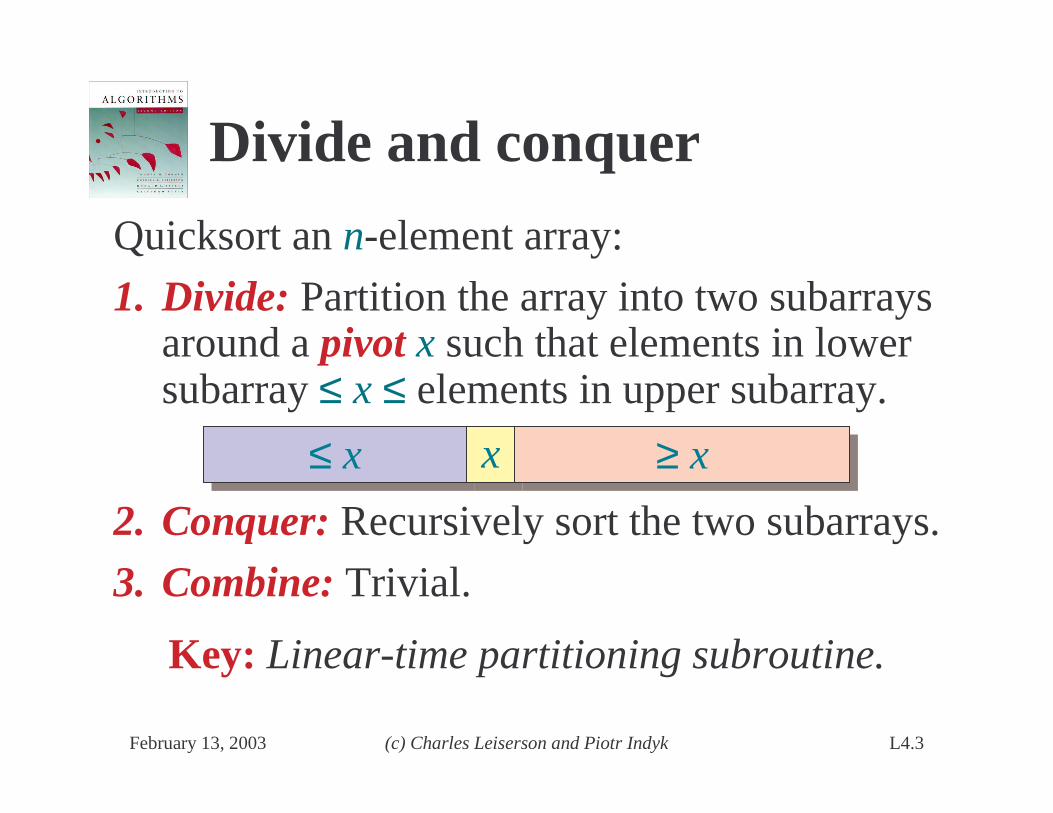
Quicksort an n-element array:
1. Divide: Partition the array into two subarrays around a pivot x such that elements in lower subarray ≤ x ≤ elements in upper subarray.
2. Conquer: Recursively sort the two subarrays.
3. Combine: Trivial.
≤ x≤ x xx ≥ x≥ x
Key: Linear-time partitioning subroutine.

February 13, 2003 (c) Charles Leiserson and Piotr Indyk L4.4
xx
Running time= O(n) for nelements.
Running time= O(n) for nelements.
Partitioning subroutinePARTITION(A, p, q) A[ p . . q]
x ← A[ p] pivot = A[ p]i ← pfor j ← p + 1 to q
do if A[ j] ≤ xthen i ← i + 1
exchangeA[i] ↔ A[ j]exchangeA[ p] ↔ A[i]return i
≤ x≤ x ≥ x≥ x ??p i qj
Invariant:

February 13, 2003 (c) Charles Leiserson and Piotr Indyk L4.5
Example of par titioning
i j66 1010 1313 55 88 33 22 1111

February 13, 2003 (c) Charles Leiserson and Piotr Indyk L4.6
Example of par titioning
i j66 1010 1313 55 88 33 22 1111

February 13, 2003 (c) Charles Leiserson and Piotr Indyk L4.7
Example of par titioning
i j66 1010 1313 55 88 33 22 1111

February 13, 2003 (c) Charles Leiserson and Piotr Indyk L4.8
Example of par titioning
66 1010 1313 55 88 33 22 1111
i j66 55 1313 1010 88 33 22 1111

February 13, 2003 (c) Charles Leiserson and Piotr Indyk L4.9
Example of par titioning
66 1010 1313 55 88 33 22 1111
i j66 55 1313 1010 88 33 22 1111

February 13, 2003 (c) Charles Leiserson and Piotr Indyk L4.10
Example of par titioning
66 1010 1313 55 88 33 22 1111
i j66 55 1313 1010 88 33 22 1111

February 13, 2003 (c) Charles Leiserson and Piotr Indyk L4.11
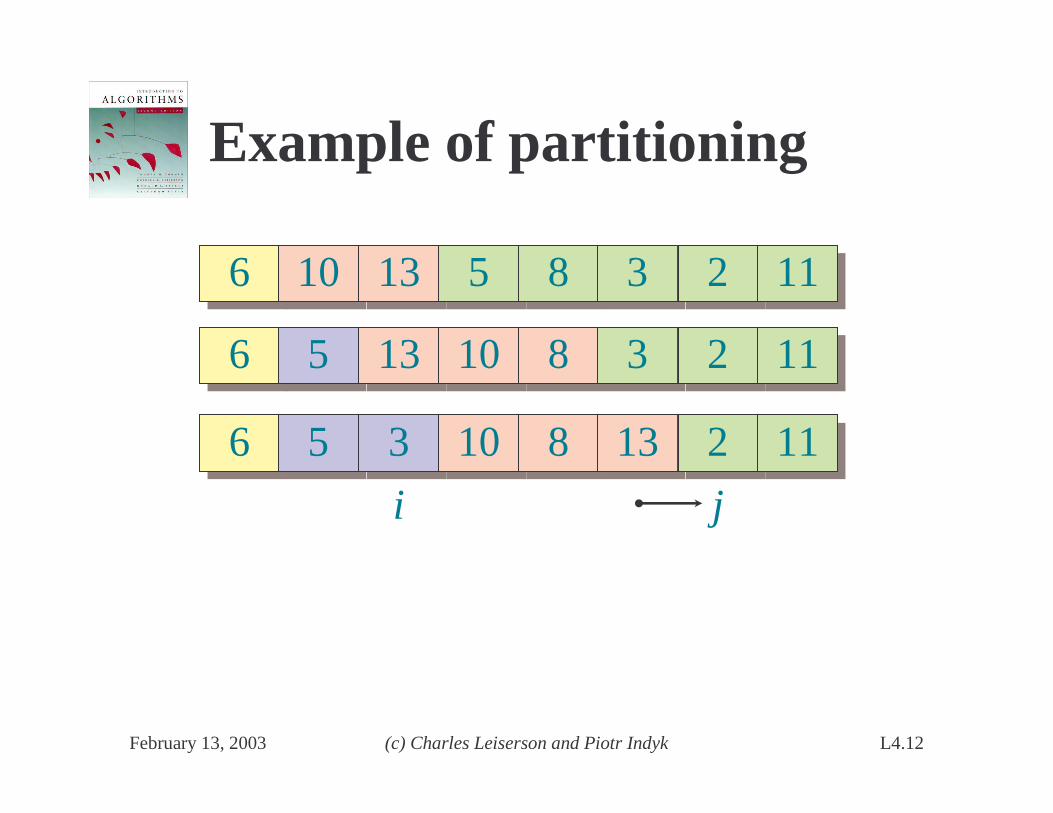
Example of par titioning
66 1010 1313 55 88 33 22 1111
i j66 55 33 1010 88 1313 22 1111
66 55 1313 1010 88 33 22 1111
February 13, 2003 (c) Charles Leiserson and Piotr Indyk L4.12
Example of par titioning
66 1010 1313 55 88 33 22 1111
i j66 55 33 1010 88 1313 22 1111
66 55 1313 1010 88 33 22 1111

February 13, 2003 (c) Charles Leiserson and Piotr Indyk L4.13
Example of par titioning
66 1010 1313 55 88 33 22 1111
66 55 33 1010 88 1313 22 1111
66 55 1313 1010 88 33 22 1111
i j66 55 33 22 88 1313 1010 1111

February 13, 2003 (c) Charles Leiserson and Piotr Indyk L4.14
Example of par titioning
66 1010 1313 55 88 33 22 1111
66 55 33 1010 88 1313 22 1111
66 55 1313 1010 88 33 22 1111
i j66 55 33 22 88 1313 1010 1111

February 13, 2003 (c) Charles Leiserson and Piotr Indyk L4.15
Example of par titioning
66 1010 1313 55 88 33 22 1111
66 55 33 1010 88 1313 22 1111
66 55 1313 1010 88 33 22 1111
i j66 55 33 22 88 1313 1010 1111
February 13, 2003 (c) Charles Leiserson and Piotr Indyk L4.16
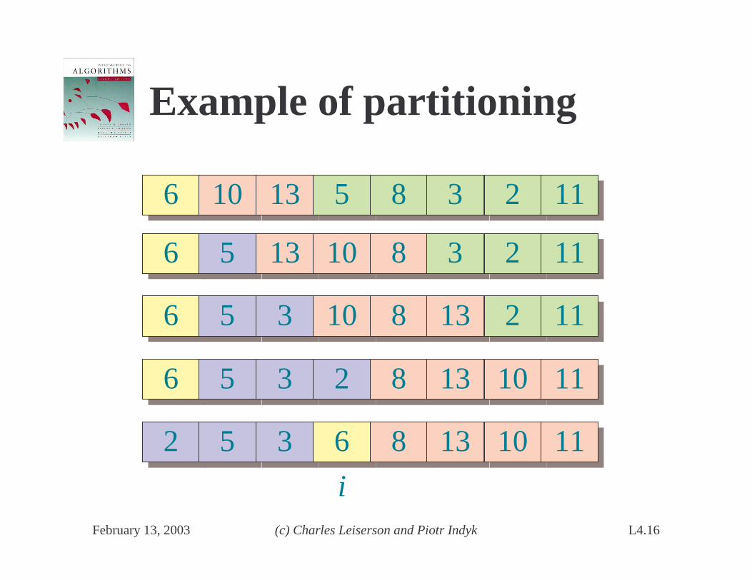
Example of par titioning
66 1010 1313 55 88 33 22 1111
66 55 33 1010 88 1313 22 1111
66 55 1313 1010 88 33 22 1111
66 55 33 22 88 1313 1010 1111
i22 55 33 66 88 1313 1010 1111

February 13, 2003 (c) Charles Leiserson and Piotr Indyk L4.17
Pseudocode for quicksor t
QUICKSORT(A, p, r)if p < r
then q ← PARTITION(A, p, r)QUICKSORT(A, p, q–1)QUICKSORT(A, q+1, r)
Initial call: QUICKSORT(A, 1, n)

February 13, 2003 (c) Charles Leiserson and Piotr Indyk L4.18
Analysis of quicksor t
• Assume all input elements are distinct.
• In practice, there are better partitioning algorithms for when duplicate input elements may exist.
• Let T(n) = worst-case running time on an array of n elements.

February 13, 2003 (c) Charles Leiserson and Piotr Indyk L4.19
Worst-case of quicksor t
• Input sorted or reverse sorted.• Partition around min or max element.• One side of partition always has no elements.
)(
)()1(
)()1()1(
)()1()0()(
2n
nnT
nnT
nnTTnT
Θ=Θ+−=
Θ+−+Θ=Θ+−+=
(arithmetic series)

February 13, 2003 (c) Charles Leiserson and Piotr Indyk L4.20
Worst-case recursion treeT(n) = T(0) + T(n–1) + cn

February 13, 2003 (c) Charles Leiserson and Piotr Indyk L4.21
Worst-case recursion treeT(n) = T(0) + T(n–1) + cn
T(n)

February 13, 2003 (c) Charles Leiserson and Piotr Indyk L4.22
cn
T(0) T(n–1)
Worst-case recursion treeT(n) = T(0) + T(n–1) + cn

February 13, 2003 (c) Charles Leiserson and Piotr Indyk L4.23
cn
T(0) c(n–1)
Worst-case recursion treeT(n) = T(0) + T(n–1) + cn
T(0) T(n–2)

February 13, 2003 (c) Charles Leiserson and Piotr Indyk L4.24
cn
T(0) c(n–1)
Worst-case recursion treeT(n) = T(0) + T(n–1) + cn
T(0) c(n–2)
T(0)
Θ(1)
�

February 13, 2003 (c) Charles Leiserson and Piotr Indyk L4.25
cn
T(0) c(n–1)
Worst-case recursion treeT(n) = T(0) + T(n–1) + cn
T(0) c(n–2)
T(0)
Θ(1)
�
( )2
1
nkn
k
Θ=���
����
�Θ �
=

February 13, 2003 (c) Charles Leiserson and Piotr Indyk L4.26
cn
Θ(1) c(n–1)
Worst-case recursion treeT(n) = T(0) + T(n–1) + cn
Θ(1) c(n–2)
Θ(1)
Θ(1)
�
( )2
1
nkn
k
Θ=���
����
�Θ �
=
T(n) = Θ(n) + Θ(n2)= Θ(n2)
h = n

February 13, 2003 (c) Charles Leiserson and Piotr Indyk L4.27
Best-case analysis(For intuition only! )
If we’ re lucky, PARTITION splits the array evenly:
T(n) = 2T(n/2) + Θ(n)= Θ(n lg n) (same as merge sort)
What if the split is always 109
101 : ?
( ) ( ) )()(109
101 nnTnTnT Θ++=
What is the solution to this recurrence?
February 13, 2003 (c) Charles Leiserson and Piotr Indyk L4.28
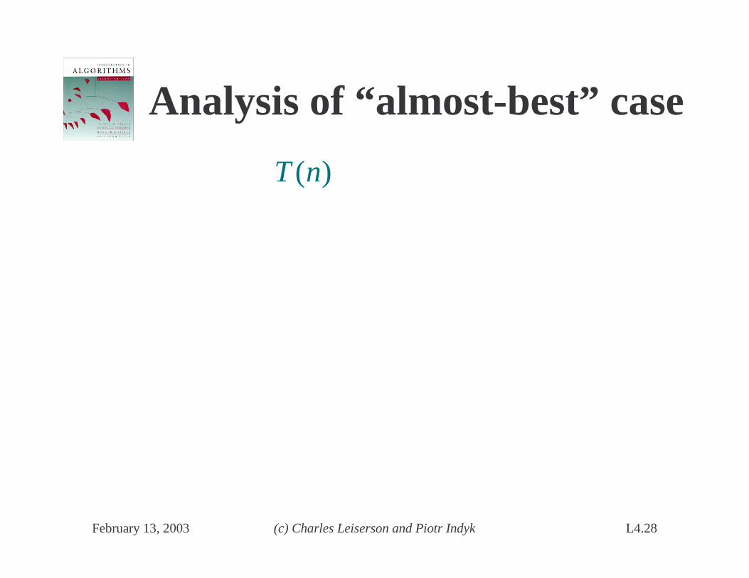
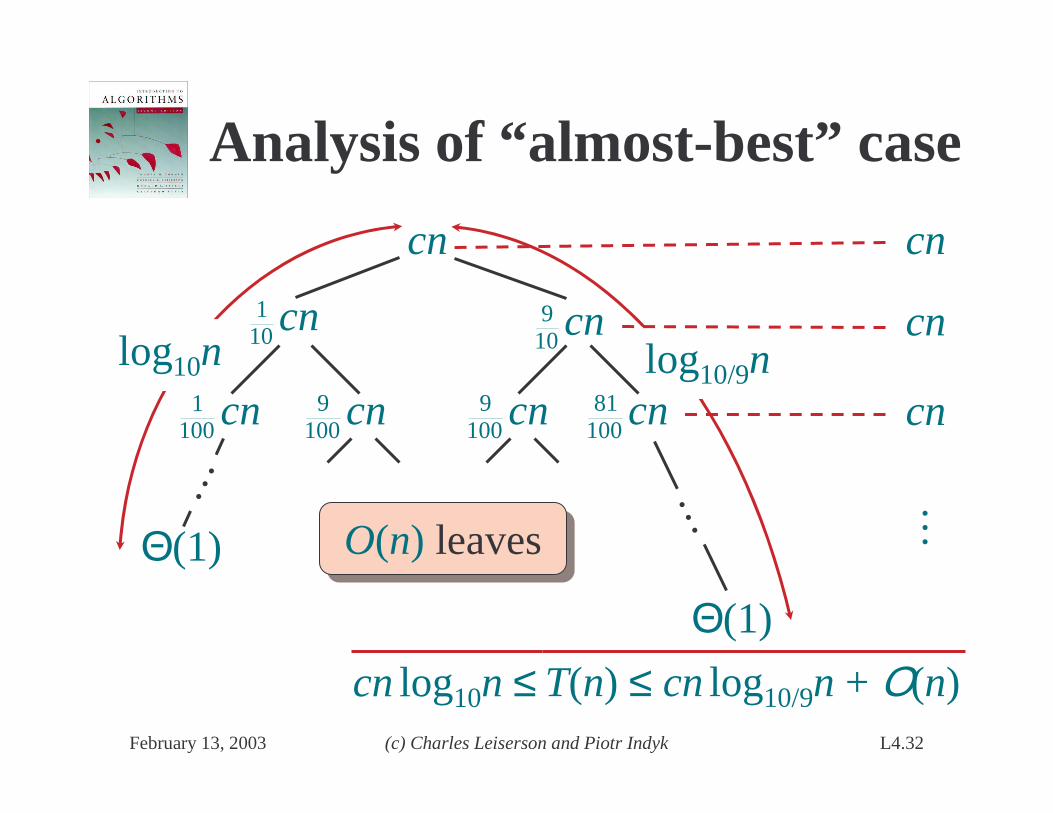
Analysis of “ almost-best” case
)(nT

February 13, 2003 (c) Charles Leiserson and Piotr Indyk L4.29
Analysis of “ almost-best” case
cn
( )nT101 ( )nT
109

February 13, 2003 (c) Charles Leiserson and Piotr Indyk L4.30
Analysis of “ almost-best” case
cn
cn101 cn
109
( )nT1001 ( )nT
1009 ( )nT
1009 ( )nT
10081

February 13, 2003 (c) Charles Leiserson and Piotr Indyk L4.31
Analysis of “ almost-best” case
cn
cn101 cn
109
cn1001 cn
1009 cn
1009 cn
10081
Θ(1)
Θ(1)
… …log10/9n
cn
cn
cn
…O(n) leavesO(n) leaves
February 13, 2003 (c) Charles Leiserson and Piotr Indyk L4.32
log10n
Analysis of “ almost-best” case
cn
cn101 cn
109
cn1001 cn
1009 cn
1009 cn
10081
Θ(1)
Θ(1)
… …log10/9n
cn
cn
cn
T(n) ≤ cn log10/9n + Ο(n)
…
cn log10n ≤
O(n) leavesO(n) leaves

February 13, 2003 (c) Charles Leiserson and Piotr Indyk L4.33
Randomized quicksor t
IDEA: Partition around a random element. I.e., around A[t] , where t chosen uniformly at random from {p…r}

February 13, 2003 (c) Charles Leiserson and Piotr Indyk L4.34
Randomized Algor ithms
• Algorithms that make decisions based on random coin flips.
• Can “ fool” the adversary.
• The running time (or even correctness) is a random variable; we measure the expectedrunning time.
• We assume all random choices are independent .
• This is not the average case !

February 13, 2003 (c) Charles Leiserson and Piotr Indyk L4.35
“ Paranoid” quicksor t
• Will modify the algorithm to make it easier to analyze:
• Repeat:• Choose the pivot at random• Perform PARTITION
• Until the resulting split is lucky, i.e., not worse than 1/10: 9/10• Recurseon both subarrays

February 13, 2003 (c) Charles Leiserson and Piotr Indyk L4.36
Analysis
• Let T(n) be an upper bound on the expectedrunning time on any array of n elements
• Consider any input of size n
• The time needed to sort the input is bounded from the above by a sum of
• The time needed to sort the left subarray
• The time needed to sort the right subarray
• The number of iterations until we get a lucky split, times cn

February 13, 2003 (c) Charles Leiserson and Piotr Indyk L4.37
Expectations
cnpartitionsEinTiTnT •+−+≤ ][#)()(max)(
• By linearity of expectation:
where maximum is taken over i ∈ [n/10,9n/10]
• We will show that E[#partitions] is less than 2
• Therefore:
]10/9,10/[,2)()(max)( nnicninTiTnT ∈+−+≤

February 13, 2003 (c) Charles Leiserson and Piotr Indyk L4.38
Final bound
• Can use the recursion tree argument:
• Tree depth is Θ(log n)
• Total work at each level is at most 2cn
• The total expected time is Ο(n log n)

February 13, 2003 (c) Charles Leiserson and Piotr Indyk L4.39
Lucky par titions
• The probability that a random pivot induces lucky partition is at least 8/10
(we are not lucky if the pivot happens to be among the smallest/largest n/10 elements)
• If we flip a coin, with heads prob. p=8/10 , the expected waiting time for the first head is 1/p = 10/8 < 2
February 13, 2003 (c) Charles Leiserson and Piotr Indyk L4.40
Quicksor t in practice
• Quicksort is a great general-purpose sorting algorithm.
• Quicksort is typically over twice as fast as merge sort.
• Quicksort can benefit substantially from code tuning.
• Quicksort behaves well even with caching and virtual memory.

February 13, 2003 (c) Charles Leiserson and Piotr Indyk L4.41
More intuition
Suppose we alternate lucky, unlucky, lucky, unlucky, lucky, ….
L(n) = 2U(n/2) + Θ(n) luckyU(n) = L(n – 1) + Θ(n) unlucky
Solving:L(n) = 2(L(n/2 – 1) + Θ(n/2)) + Θ(n)
= 2L(n/2 – 1) + Θ(n)= Θ(n lg n)
How can we make sure we are usually lucky?
Lucky!

February 13, 2003 (c) Charles Leiserson and Piotr Indyk L4.42
Randomized quicksor t analysis
Let T(n) = the random variable for the running time of randomized quicksort on an input of size n, assuming random numbers are independent.
For k = 0, 1, …, n–1, define the indicator random variable
Xk =1 if PARTITION generates a k : n–k–1 split,0 otherwise.
E[Xk] = Pr{ Xk = 1} = 1/n, since all splits are equally likely, assuming elements are distinct.

February 13, 2003 (c) Charles Leiserson and Piotr Indyk L4.43
Analysis (continued)
T(n) =
T(0) + T(n–1) + Θ(n) if 0 : n–1 split,T(1) + T(n–2) + Θ(n) if 1 : n–2 split,
�
T(n–1) + T(0) + Θ(n) if n–1 : 0 split,
( )�−
=Θ+−−+=
1
0
)()1()(n
kk nknTkTX .

February 13, 2003 (c) Charles Leiserson and Piotr Indyk L4.44
Calculating expectation
( )�
��
Θ+−−+= �
−
=
1
0
)()1()()]([n
kk nknTkTXEnTE
Take expectations of both sides.

February 13, 2003 (c) Charles Leiserson and Piotr Indyk L4.45
Calculating expectation
( )
( )[ ]�
�
−
=
−
=
Θ+−−+=
�
��
Θ+−−+=
1
0
1
0
)()1()(
)()1()()]([
n
kk
n
kk
nknTkTXE
nknTkTXEnTE
Linearity of expectation.

February 13, 2003 (c) Charles Leiserson and Piotr Indyk L4.46
Calculating expectation
( )
( )[ ]
[ ] [ ]�
�
�
−
=
−
=
−
=
Θ+−−+⋅=
Θ+−−+=
�
��
Θ+−−+=
1
0
1
0
1
0
)()1()(
)()1()(
)()1()()]([
n
kk
n
kk
n
kk
nknTkTEXE
nknTkTXE
nknTkTXEnTE
Independence of Xk from other random choices.

February 13, 2003 (c) Charles Leiserson and Piotr Indyk L4.47
Calculating expectation
( )
( )[ ]
[ ] [ ]
[ ] [ ] ���
�
�
�
−
=
−
=
−
=
−
=
−
=
−
=
Θ+−−+=
Θ+−−+⋅=
Θ+−−+=
�
��
Θ+−−+=
1
0
1
0
1
0
1
0
1
0
1
0
)(1)1(1)(1
)()1()(
)()1()(
)()1()()]([
n
k
n
k
n
k
n
kk
n
kk
n
kk
nn
knTEn
kTEn
nknTkTEXE
nknTkTXE
nknTkTXEnTE
Linearity of expectation; E[Xk] = 1/n .

February 13, 2003 (c) Charles Leiserson and Piotr Indyk L4.48
Calculating expectation
( )
( )[ ]
[ ] [ ]
[ ] [ ]
[ ] )()(2
)(1)1(1)(1
)()1()(
)()1()(
)()1()()]([
1
1
1
0
1
0
1
0
1
0
1
0
1
0
nkTEn
nn
knTEn
kTEn
nknTkTEXE
nknTkTXE
nknTkTXEnTE
n
k
n
k
n
k
n
k
n
kk
n
kk
n
kk
Θ+=
Θ+−−+=
Θ+−−+⋅=
Θ+−−+=
�
��
Θ+−−+=
�
���
�
�
�
−
=
−
=
−
=
−
=
−
=
−
=
−
=
Summations have identical terms.

February 13, 2003 (c) Charles Leiserson and Piotr Indyk L4.49
Hairy recurrence
[ ] )()(2)]([1
2
nkTEn
nTEn
k
Θ+= �−
=
(The k = 0, 1 terms can be absorbed in the Θ(n).)
Prove: E[T(n)] ≤ an lgn for constant a > 0.
Use fact: 21
2812
21 lglg nnnkk
n
k�
−
=−≤ (exercise).
• Choose a large enough so that an lgndominates E[T(n)] for sufficiently small n ≥ 2.

February 13, 2003 (c) Charles Leiserson and Piotr Indyk L4.50
Substitution method
[ ] )(lg2)(1
2
nkakn
nTEn
k
Θ+≤ �−
=
Substitute inductive hypothesis.

February 13, 2003 (c) Charles Leiserson and Piotr Indyk L4.51
Substitution method
[ ]
)(81lg
212
)(lg2)(
22
1
2
nnnnna
nkakn
nTEn
k
Θ+����
�� −≤
Θ+≤ �−
=
Use fact.

February 13, 2003 (c) Charles Leiserson and Piotr Indyk L4.52
Substitution method
[ ]
����
�� Θ−−=
Θ+����
�� −≤
Θ+≤ �−
=
)(4
lg
)(81lg
212
)(lg2)(
22
1
2
nannan
nnnnna
nkakn
nTEn
k
Express as desired – residual.

February 13, 2003 (c) Charles Leiserson and Piotr Indyk L4.53
Substitution method
[ ]
nan
nannan
nnnnna
nkakn
nTEn
k
lg
)(4
lg
)(81lg
212
)(lg2)(
22
1
2
≤
����
�� Θ−−=
Θ+����
�� −=
Θ+≤ �−
=
if a is chosen large enough so that an/4 dominates the Θ(n).
,

February 13, 2003 (c) Charles Leiserson and Piotr Indyk L4.54
• Assume