introduction to analytic perspectives spatial...

1

Introduction toSpatial Analysis

II. Spatial analysis of latticedataStuart SweeneyGEOG 172, Fall 2007

2

Module organization Basic concepts Analytic perspectives Space as container Space as indicator

Spatial dependence/autocorrelation Global Moran’s I Local Moran’s I

Spatial econometric models

3

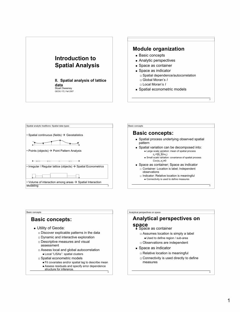
• Spatial continuous (fields) Geostatistics

• Points (objects) Point Pattern Analysis

• Irregular / Regular lattice (objects) Spatial Econometrics

• Volume of interaction among areas Spatial InteractionModeling

Spatial analytic traditions: Spatial data types

4

Spatial process underlying observed spatialpattern

Spatial variation can be decomposed into: Large scale variation: mean of spatial process

zs=f(Xs’B+es) Small scale variation: covariance of spatial process

Cov(ei,ej)=0

Space as container; Space as indicator Container: Location is label; Independent

observations Indicator: Relative location is meaningful

Connectivity is used to define measures

Basic concepts:

/

Basic concepts

5

Utility of Geoda: Discover explicable patterns in the data Dynamic and interactive exploration Descriptive measures and visual

assessment Assess local and global autocorrelation

Local “LISAs”: spatial clusters Spatial econometric models

Fit covariates and/or spatial lag to describe mean Assess residuals and specify error dependence

structure for inference.

Basic concepts:Basic concepts

6

Space as container Assumes location is simply a label

Used to define region / sub-area Observations are independent

Space as indicator Relative location is meaningful Connectivity is used directly to define

measures

Analytical perspectives onspace

Analytical perspectives on space

2

7

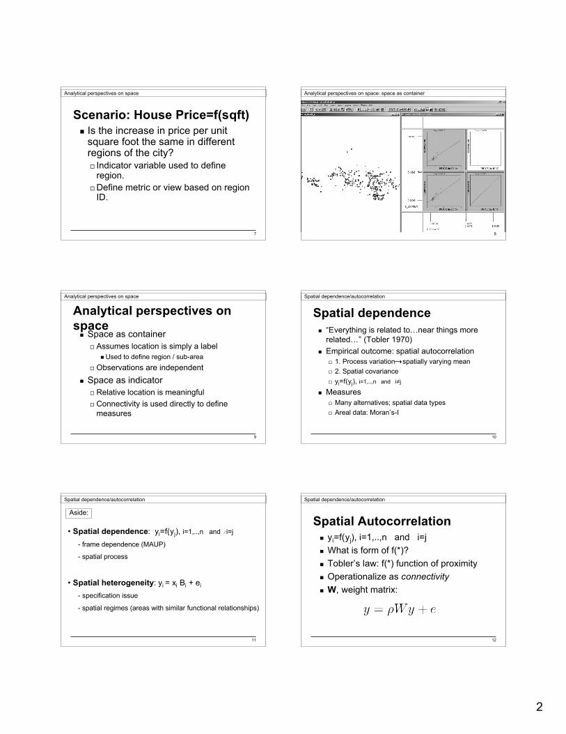
Scenario: House Price=f(sqft) Is the increase in price per unit

square foot the same in differentregions of the city? Indicator variable used to define

region. Define metric or view based on region

ID.


8

Space as container

Analytical perspectives on space: space as container

9

Space as container Assumes location is simply a label

Used to define region / sub-area Observations are independent

Space as indicator Relative location is meaningful Connectivity is used directly to define

measures

Analytical perspectives onspace


10

“Everything is related to…near things morerelated…” (Tobler 1970)

Empirical outcome: spatial autocorrelation 1. Process variation spatially varying mean 2. Spatial covariance yi=f(yj), i=1,..,n and i=j

Measures Many alternatives; spatial data types Areal data: Moran’s-I

Spatial dependenceSpatial dependence/autocorrelation

11

• Spatial dependence: yi=f(yj), i=1,..,n and i=j

- frame dependence (MAUP)

- spatial process

• Spatial heterogeneity: yi = xi Bi + ei

- specification issue

- spatial regimes (areas with similar functional relationships)

Spatial dependence/autocorrelation

Aside:

12

yi=f(yj), i=1,..,n and i=j What is form of f(*)? Tobler’s law: f(*) function of proximity Operationalize as connectivity W, weight matrix:

Spatial Autocorrelation


3

13

1 23

45

67

Connectivity example: Map of seven areas

Share border: Neighbor(1)={2,3,4,7}Neighbor(2)={1,3}..Neighbor(7)={1,3,6}

1 23

4

5

67

Recall:

W=~

0 1 1 1 0 0 11 0 1 0 0 0 01 1 0 1 1 1 11 0 1 0 1 0 00 0 1 1 0 1 00 0 1 0 1 0 11 0 1 0 0 1 0


14

Spatial Autocorrelation (cont.)Binary W matrix: Row standardized W matrix:


15

Geoda: W matrix


16

Read shapefile directly Can view properties of W matrix Can easily create multiple for sensitivity

analysis Can open and directly edit .GAL file

Demo I: Creating W matrix


17

Select: Tools>Weights>Create Input file: C:\temp\sbreal_tract_p.shp Output file: C:\temp\sbtrct_rook.gal Select “rook”, click on create

Select: Tools>Weights>Properties Open sbtrct_rook.gal in a text editor

(Notepad)

Application: Working with W


18

Activity: Map to W Draw an outline map containing eight

areas/regions. Write the numbers 1 through 8 in the

eight areas. Give the map to your neighbor. Write down the first two rows of the W

matrix using your neighbors map. Use arook contiguity rule.

Exchange maps with a different neighborand check each others work.

4

19

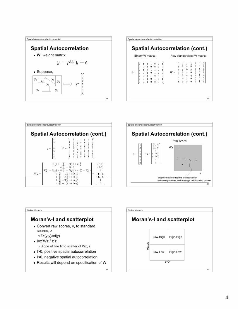
W, weight matrix:

Suppose,

Spatial Autocorrelation


y1 y2y3

y4 y5

y6y7

y=

20

Spatial Autocorrelation (cont.)Binary W matrix: Row standardized W matrix:


21

Spatial Autocorrelation (cont.)


22

Spatial Autocorrelation (cont.)Plot Wy, y:

Slope indicates degree of associationbetween y values and average neighboring values

Wy

y


23

Convert raw scores, y, to standardscores, z Z=(y-y)/sd(y)

I=z’Wz / z’z Slope of line fit to scatter of Wz, z

I>0, positive spatial autocorrelation I<0, negative spatial autocorrelation Results will depend on specification of W

Moran’s-I and scatterplot

Global Moran’s

24


z=0

Wz=

0

High-HighLow-High

High-LowLow-Low

Global Moran’s

5

25

W specification:


“The specification of which elements arenonzero in the spatial weights matrix is amatter of considerable arbitrariness and awide range of suggestions have been offeredin the literature.” Anselin and Bera (1998)

Global Moran’s

26

• first order contiguity: wij=1 if common border, 0 otherwise.

• Cliff-Ord weights:

• Spatial interaction / potential weights:

• Social or economic distance:

• Need to be exogenous and satisfy regularity conditions.

Aside: Alternative Weights Matrices

Global Moran’s

27

Geoda: Moran’s-I, scatterplotGlobal Moran’s

28

Visual and numeric assessment ofspatial autocorrelation

Visual assessment of distributionalassumptions Z-scores implies symmetric dist. Is your variable approximately symmetric?

Sensitivity analysis / leverage analysis

Demo II: Moran scatterplot

Global Moran’s

29

I=z’Wz / z’z I>0, positive spatial autocorrelation I<0, negative spatial autocorrelation Questions:

What does I>0 mean? Inference: Is significantly different from 0?

Ho: I=0, Ha:I>0

Moran’s-I: Interpretation

Global Moran’s

30

Moran’s-I: Interpretation

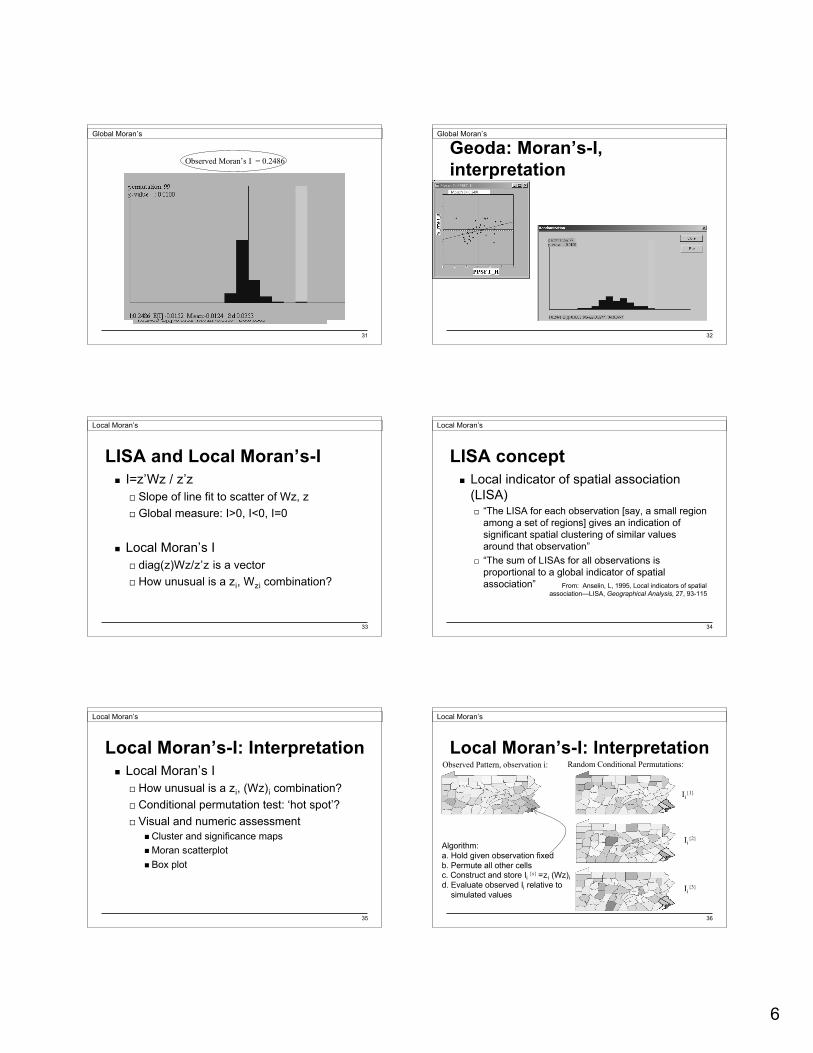
Observed Moran’s I = 0.2486

Observed Pattern: Random Permutations:

I{1} =0.0290

I{2} =0.0232

I{3} =0.0525

Global Moran’s

6

31

Observed Moran’s I = 0.2486

Global Moran’s

32

Geoda: Moran’s-I,interpretation

Global Moran’s

33

I=z’Wz / z’z Slope of line fit to scatter of Wz, z Global measure: I>0, I<0, I=0

Local Moran’s I diag(z)Wz/z’z is a vector How unusual is a zi, Wzi combination?

LISA and Local Moran’s-I

Local Moran’s

34

LISA concept Local indicator of spatial association

(LISA) “The LISA for each observation [say, a small region

among a set of regions] gives an indication ofsignificant spatial clustering of similar valuesaround that observation”

“The sum of LISAs for all observations isproportional to a global indicator of spatialassociation” From: Anselin, L, 1995, Local indicators of spatial

association—LISA, Geographical Analysis, 27, 93-115

Local Moran’s

35

Local Moran’s I How unusual is a zi, (Wz)i combination? Conditional permutation test: ‘hot spot’? Visual and numeric assessment

Cluster and significance maps Moran scatterplot Box plot

Local Moran’s-I: Interpretation

Local Moran’s

36

Local Moran’s-I: InterpretationObserved Pattern, observation i: Random Conditional Permutations:

Ii{1}

Ii{2}

Ii{3}

Algorithm:a. Hold given observation fixedb. Permute all other cellsc. Construct and store Ii {s}

=zi (Wz)id. Evaluate observed Ii relative to simulated values

Local Moran’s

7

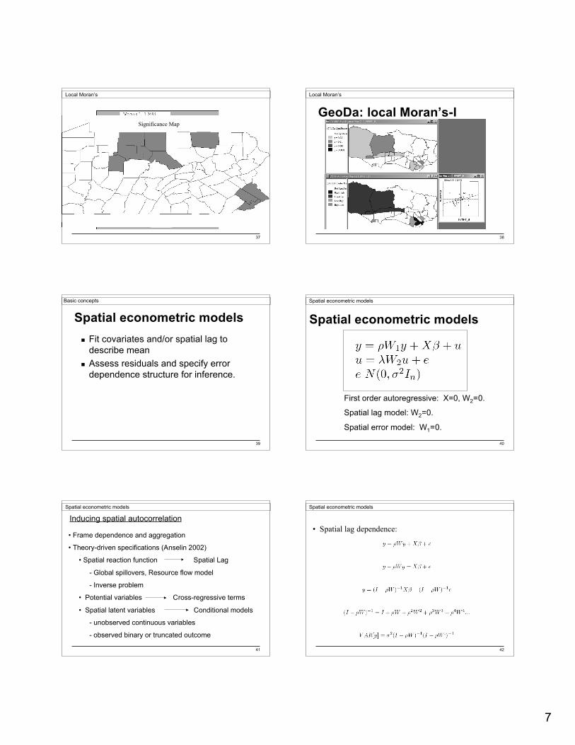
37

Cluster MapSignificance Map

Local Moran’s

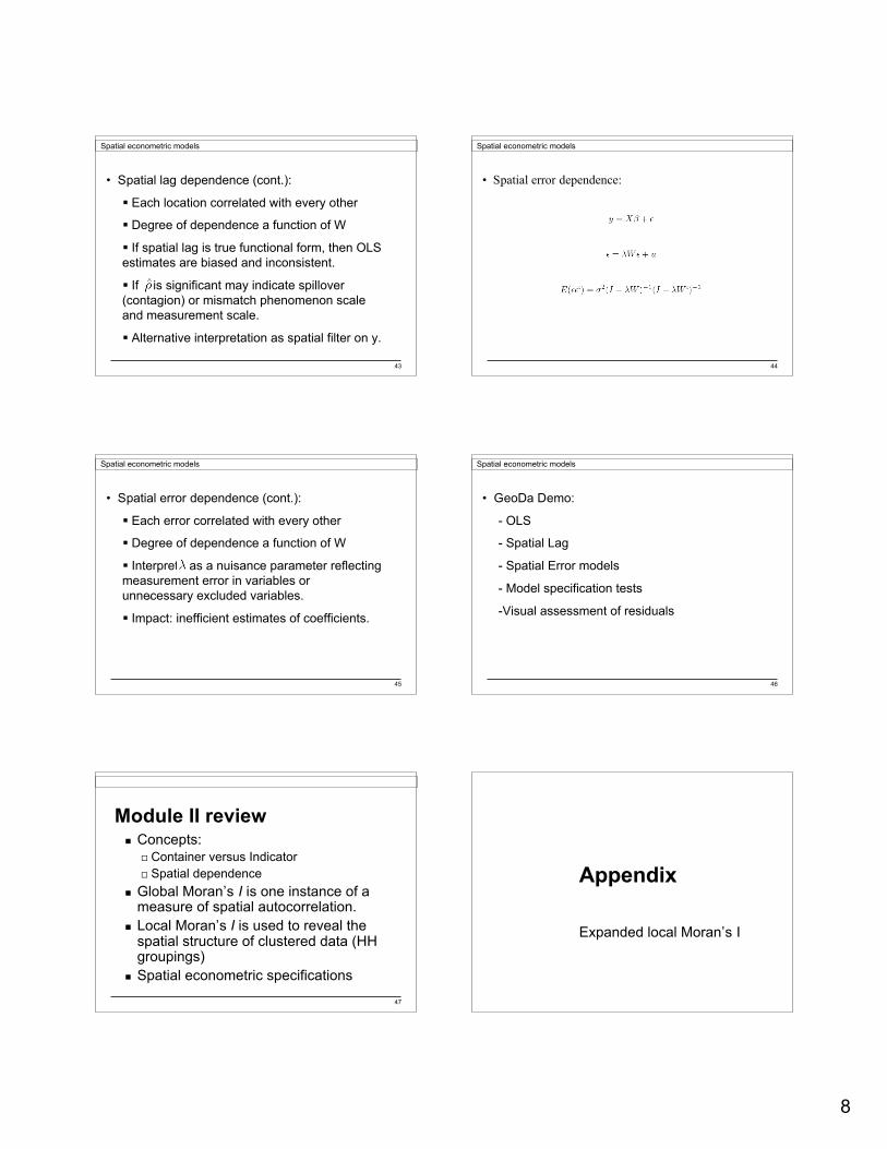
38

GeoDa: local Moran’s-ILocal Moran’s

39

Fit covariates and/or spatial lag todescribe mean

Assess residuals and specify errordependence structure for inference.

Spatial econometric modelsBasic concepts

40

First order autoregressive: X=0, W2=0.

Spatial lag model: W2=0.

Spatial error model: W1=0.



41

• Frame dependence and aggregation

• Theory-driven specifications (Anselin 2002)

• Spatial reaction function Spatial Lag

- Global spillovers, Resource flow model

- Inverse problem

• Potential variables Cross-regressive terms

• Spatial latent variables Conditional models

- unobserved continuous variables

- observed binary or truncated outcome

Inducing spatial autocorrelationSpatial econometric models

42

• Spatial lag dependence:


8

43

• Spatial lag dependence (cont.):

Each location correlated with every other

Degree of dependence a function of W

If spatial lag is true functional form, then OLSestimates are biased and inconsistent.

If is significant may indicate spillover(contagion) or mismatch phenomenon scaleand measurement scale.

Alternative interpretation as spatial filter on y.

^


44

• Spatial error dependence:


45

• Spatial error dependence (cont.):

Each error correlated with every other

Degree of dependence a function of W

Interpret as a nuisance parameter reflectingmeasurement error in variables orunnecessary excluded variables.

Impact: inefficient estimates of coefficients.^


46

• GeoDa Demo:

- OLS

- Spatial Lag

- Spatial Error models

- Model specification tests

-Visual assessment of residuals


47

Module II review Concepts:

Container versus Indicator Spatial dependence

Global Moran’s I is one instance of ameasure of spatial autocorrelation.

Local Moran’s I is used to reveal thespatial structure of clustered data (HHgroupings)

Spatial econometric specifications

Appendix

Expanded local Moran’s I

9

49

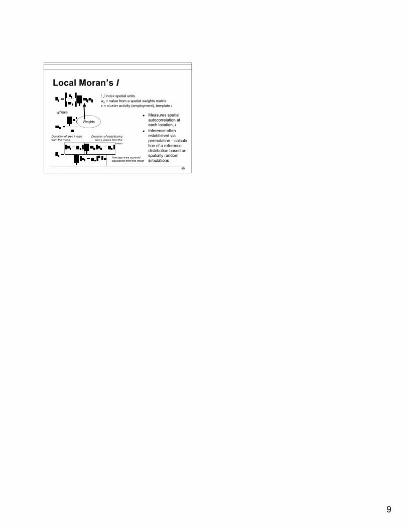
Local Moran’s I

Measures spatialautocorrelation ateach location, i

Inference oftenestablished viapermutation—calculation of a referencedistribution based onspatially randomsimulations

i, j index spatial unitswij = value from a spatial weights matrixx = cluster activity (employment), template i

Weights

where

Deviation of area i valuefrom the mean

Deviation of neighboringarea j values from the

mean

Average area squareddeviations from the mean

introduction to analytic perspectives spatial...

Documents