introduction to arules – a computational environment for mining
TRANSCRIPT

Introduction to arules – A computational
environment for mining association rules and
frequent item sets
Michael Hahsler
Southern Methodist UniversityBettina Grun
Johannes Kepler Universitat Linz
Kurt Hornik
Wirtschaftsuniversitat WienChristian Buchta
Wirtschaftsuniversitat Wien
Abstract
Mining frequent itemsets and association rules is a popular and well researched ap-proach for discovering interesting relationships between variables in large databases. TheR package arules presented in this paper provides a basic infrastructure for creating andmanipulating input data sets and for analyzing the resulting itemsets and rules. The pack-age also includes interfaces to two fast mining algorithms, the popular C implementationsof Apriori and Eclat by Christian Borgelt. These algorithms can be used to mine frequentitemsets, maximal frequent itemsets, closed frequent itemsets and association rules.
Keywords: data mining, association rules, apriori, eclat.
1. Introduction
Mining frequent itemsets and association rules is a popular and well researched method for dis-covering interesting relations between variables in large databases. Piatetsky-Shapiro (1991)describes analyzing and presenting strong rules discovered in databases using different mea-sures of interestingness. Based on the concept of strong rules, Agrawal, Imielinski, and Swami(1993) introduced the problem of mining association rules from transaction data as follows:
Let I = {i1, i2, . . . , in} be a set of n binary attributes called items. Let D = {t1, t2, . . . , tm}be a set of transactions called the database. Each transaction in D has an unique transactionID and contains a subset of the items in I. A rule is defined as an implication of the formX ⇒ Y where X,Y ⊆ I and X ∩ Y = ∅. The sets of items (for short itemsets) X and Yare called antecedent (left-hand-side or LHS) and consequent (right-hand-side or RHS) of therule.
To illustrate the concepts, we use a small example from the supermarket domain. The set ofitems is I = {milk, bread, butter, beer} and a small database containing the items is shown inFigure 1. An example rule for the supermarket could be {milk, bread} ⇒ {butter} meaningthat if milk and bread is bought, customers also buy butter.
To select interesting rules from the set of all possible rules, constraints on various measures of

2 Introduction to arules
significance and interest can be used. The best-known constraints are minimum thresholds onsupport and confidence. The support supp(X) of an itemset X is defined as the proportion oftransactions in the data set which contain the itemset. In the example database in Figure 1,the itemset {milk, bread} has a support of 2/5 = 0.4 since it occurs in 40% of all transactions(2 out of 5 transactions).
Finding frequent itemsets can be seen as a simplification of the unsupervised learning problemcalled “mode finding” or “bump hunting” (Hastie, Tibshirani, and Friedman 2001). For theseproblems each item is seen as a variable. The goal is to find prototype values so that theprobability density evaluated at these values is sufficiently large. However, for practicalapplications with a large number of variables, probability estimation will be unreliable andcomputationally too expensive. This is why in practice frequent itemsets are used instead ofprobability estimation.
The confidence of a rule is defined conf(X ⇒ Y ) = supp(X ∪ Y )/supp(X). For example, therule {milk, bread} ⇒ {butter} has a confidence of 0.2/0.4 = 0.5 in the database in Figure 1,which means that for 50% of the transactions containing milk and bread the rule is correct.Confidence can be interpreted as an estimate of the probability P (Y |X), the probability offinding the RHS of the rule in transactions under the condition that these transactions alsocontain the LHS (see e.g., Hipp, Guntzer, and Nakhaeizadeh 2000).
Association rules are required to satisfy both a minimum support and a minimum confidenceconstraint at the same time. At medium to low support values, often a great number offrequent itemsets are found in a database. However, since the definition of support enforcesthat all subsets of a frequent itemset have to be also frequent, it is sufficient to only mine allmaximal frequent itemsets, defined as frequent itemsets which are not proper subsets of anyother frequent itemset (Zaki, Parthasarathy, Ogihara, and Li 1997b). Another approach toreduce the number of mined itemsets is to only mine frequent closed itemsets. An itemsetis closed if no proper superset of the itemset is contained in each transaction in which theitemset is contained (Pasquier, Bastide, Taouil, and Lakhal 1999; Zaki 2004). Frequent closeditemsets are a superset of the maximal frequent itemsets. Their advantage over maximalfrequent itemsets is that in addition to yielding all frequent itemsets, they also preserve thesupport information for all frequent itemsets which can be important for computing additionalinterest measures after the mining process is finished (e.g., confidence for rules generated fromthe found itemsets, or all-confidence (Omiecinski 2003)).
A practical solution to the problem of finding too many association rules satisfying the supportand confidence constraints is to further filter or rank found rules using additional interestmeasures. A popular measure for this purpose is lift (Brin, Motwani, Ullman, and Tsur1997). The lift of a rule is defined as lift(X ⇒ Y ) = supp(X ∪ Y )/(supp(X)supp(Y )), and
transaction ID items
1 milk, bread2 bread, butter3 beer4 milk, bread, butter5 bread, butter
Figure 1: An example supermarket database with five transactions.

Michael Hahsler, Bettina Grun, Kurt Hornik, Christian Buchta 3
can be interpreted as the deviation of the support of the whole rule from the support expectedunder independence given the supports of the LHS and the RHS. Greater lift values indicatestronger associations.
In the last decade, research on algorithms to solve the frequent itemset problem has beenabundant. Goethals and Zaki (2004) compare the currently fastest algorithms. Among thesealgorithms are the implementations of the Apriori and Eclat algorithms by Borgelt (2003)interfaced in the arules environment. The two algorithms use very different mining strategies.Apriori, developed by Agrawal and Srikant (1994), is a level-wise, breadth-first algorithmwhich counts transactions. In contrast, Eclat (Zaki et al. 1997b) employs equivalence classes,depth-first search and set intersection instead of counting. The algorithms can be used tomine frequent itemsets, maximal frequent itemsets and closed frequent itemsets. The imple-mentation of Apriori can additionally be used to generate association rules.
This paper presents arules1, an extension package for R (R Development Core Team 2005)which provides the infrastructure needed to create and manipulate input data sets for themining algorithms and for analyzing the resulting itemsets and rules. Since it is common towork with large sets of rules and itemsets, the package uses sparse matrix representationsto minimize memory usage. The infrastructure provided by the package was also created toexplicitly facilitate extensibility, both for interfacing new algorithms and for adding new typesof interest measures and associations.
The rest of the paper is organized as follows: In the next section, we give an overview of thedata structures implemented in the package arules. In Section 2 we introduce the functionalityof the classes to handle transaction data and associations. In Section 3 we describe the waymining algorithms are interfaced in arules using the available interfaces to Apriori and Eclat asexamples. In Section 4 we present some auxiliary methods for support counting, rule inductionand sampling available in arules. We provide several examples in Section 5. The first twoexamples show typical R sessions for preparing, analyzing and manipulating a transactiondata set, and for mining association rules. The third example demonstrates how arules canbe extended to integrate a new interest measure. Finally, the fourth example shows howto use sampling in order to speed up the mining process. We conclude with a summary ofthe features and strengths of the package arules as a computational environment for miningassociation rules and frequent itemsets.
A previous version of this manuscript was published in the Journal of Statistical Software(Hahsler, Grun, and Hornik 2005a).
2. Data structure overview
To enable the user to represent and work with input and output data of association rulemining algorithms in R, a well-designed structure is necessary which can deal in an efficientway with large amounts of sparse binary data. The S4 class structure implemented in thepackage arules is presented in Figure 2.
For input data the classes transactions and tidLists (transaction ID lists, an alternative wayto represent transaction data) are provided. The output of the mining algorithms comprisesthe classes itemsets and rules representing sets of itemsets or rules, respectively. Both classes
1The arules package can be obtained from http://CRAN.R-Project.org and the maintainer can be contacted

4 Introduction to arules
associations
quality : data.frame
itemsets rules
itemMatrix
itemInfo : data.frame
tidLists
itemInfo : data.frame
transactionInfo : data.frame
Matrix
ngCMatrix
transactions
transactionInfo : data.frame
ASparameter
ECparameter APparameter
AScontrol
APcontrol ECcontrol
20..1
Figure 2: UML class diagram (see Fowler 2004) of the arules package.
directly extend a common virtual class called associations which provides a common interface.In this structure it is easy to add a new type of associations by adding a new class thatextends associations.
Items in associations and transactions are implemented by the itemMatrix class which providesa facade for the sparse matrix implementation ngCMatrix from the R package Matrix (Batesand Maechler 2005).
To control the behavior of the mining algorithms, the two classes ASparameter and AScontrol
are used. Since each algorithm can use additional algorithm-specific parameters, we imple-mented for each interfaced algorithm its own set of control classes. We used the prefix ‘AP’ forApriori and ‘EC’ for Eclat. In this way, it is easy to extend the control classes when interfacinga new algorithm.
2.1. Representing collections of itemsets
From the definition of the association rule mining problem we see that transaction databasesand sets of associations have in common that they contain sets of items (itemsets) togetherwith additional information. For example, a transaction in the database contains a transactionID and an itemset. A rule in a set of mined association rules contains two itemsets, one forthe LHS and one for the RHS, and additional quality information, e.g., values for variousinterest measures.
Collections of itemsets used for transaction databases and sets of associations can be rep-resented as binary incidence matrices with columns corresponding to the items and rowscorresponding to the itemsets. The matrix entries represent the presence (1) or absence (0) of

Michael Hahsler, Bettina Grun, Kurt Hornik, Christian Buchta 5
items
i1 i2 i3 i4milk bread butter beer
item
sets
X1 1 1 0 0
X2 0 1 0 1
X3 1 1 1 0
X4 0 0 1 0
Figure 3: Example of a collection of itemsets represented as a binary incidence matrix.
an item in a particular itemset. An example of a binary incidence matrix containing itemsetsfor the example database in Figure 1 on Page 2 is shown in Figure 3. Note that we need tostore collections of itemsets with possibly duplicated elements (identical rows), i.e, itemsetscontaining exactly the same items. This is necessary, since a transaction database can containdifferent transactions with the same items. Such a database is still a set of transactions sinceeach transaction also contains a unique transaction ID.
Since a typical frequent itemset or a typical transaction (e.g., a supermarket transaction)only contains a small number of items compared to the total number of available items, thebinary incidence matrix will in general be very sparse with many items and a very largenumber of rows. A natural representation for such data is a sparse matrix format. For ourimplementation we chose the ngCMatrix class defined in package Matrix. The ngCMatrix
is a compressed, sparse, logical, column-oriented matrix which contains the indices of theTRUE rows and the pointers to the initial indices of elements in each column of the matrix.Despite the column orientation of the ngCMatrix, it is more convenient to work with incidencematrices which are row-oriented. This makes the most important manipulation, selecting asubset of transactions from a data set for mining, more comfortable and efficient. Therefore,we implemented the class itemMatrix providing a row-oriented facade to the ngCMatrix whichstores a transposed incidence matrix2. In sparse representation the following informationneeds to be stored for the collection of itemsets in Figure 3: A vector of indices of the non-zero elements (row-wise starting with the first row) 1, 2, 2, 4, 1, 2, 3, 3 and the pointers 1, 3, 5, 8where each row starts in the index vector. The first two pointers indicate that the first rowstarts with element one in the index vector and ends with element 2 (since with element 3already the next row starts). The first two elements of the index vector represent the items inthe first row which are i1 and i2 or milk and bread, respectively. The two vectors are stored inthe ngCMatrix. Note that indices for the ngCMatrix start with zero rather than with one andthus actually the vectors 0, 1, 1, 3, 0, 3, 3 and 0, 3, 4, 7 are stored. However, the data structureof the ngCMatrix class is not intended to be directly accessed by the end user of arules. Theinterfaces of itemMatrix can be used without knowledge of how the internal representation ofthe data works. However, if necessary, the ngCMatrix can be directly accessed by developersto add functionality to arules (e.g., to develop new types of associations or interest measuresor to efficiently compute a distance matrix between itemsets for clustering). In this case, thengCMatrix should be accessed using the coercion mechanism from itemMatrix to ngCMatrix
via as().
2Note that the developers of package Matrix contains some support for a sparse row-oriented format, but
the available functionality currently is rather minimal. Once all required functionality is implemented, arules
will switch the internal representation to sparse row-oriented logical matrices.

6 Introduction to arules
In addition to the sparse matrix, itemMatrix stores item labels (e.g., names of the items) andhandles the necessary mapping between the item label and the corresponding column numberin the incidence matrix. Optionally, itemMatrix can also store additional information on items.For example, the category hierarchy in a supermarket setting can be stored which enables theanalyst to select only transactions (or as we later see also rules and itemsets) which containitems from a certain category (e.g., all dairy products).
For itemMatrix, basic matrix operations including dim() and subset selection ([) are available.The first element of dim() and [ corresponds to itemsets or transactions (rows), the secondelement to items (columns). For example, on a transaction data set in variable x the subsetselection ‘x[1:10, 16:20]’ selects a matrix containing the first 10 transactions and items 16to 20.
Since itemMatrix is used to represent sets or collections of itemsets additional functionality isprovided. length() can be used to get the number of itemsets in an itemMatrix. Technically,length() returns the number of rows in the matrix which is equal to the first element returnedby dim(). Identical itemsets can be found with duplicated(), and duplications can beremoved with unique(). match() can be used to find matching elements in two collectionsof itemsets.
With c(), several itemMatrix objects can be combined by successively appending the rowsof the objects, i.e., creating a collection of itemsets which contains the itemsets from allitemMatrix objects. This operation is only possible if the itemMatrix objects employed are“compatible,” i.e., if the matrices have the same number of columns and the items are in thesame order. If two objects contain the same items (item labels), but the order in the matrix isdifferent or one object is missing some items, recode() can be used to make them compatibleby reordering and inserting columns.
To get the actual number of items in the itemsets stored in the itemMatrix, size() is used.It returns a vector with the number of items (ones) for each element in the set (row sum inthe matrix). Obtaining the sizes from the sparse representations is a very efficient operation,since it can be calculated directly from the vector of column pointers in the ngCMatrix.For a purchase incidence matrix, size() will produce a vector as long as the number oftransactions in the matrix with each element of the vector containing the number of items inthe corresponding transaction. This information can be used, e.g., to select or filter unusuallylong or short transactions.
itemFrequency() calculates the frequency for each item in an itemMatrix. Conceptually, theitem frequencies are the column sums of the binary matrix. Technically, column sums can beimplemented for sparse representation efficiently by just tabulating the vector of row numbersof the non-zero elements in the ngCMatrix. Item frequencies can be used for many purposes.For example, they are needed to compute interest measures. itemFrequency() is also usedby itemFrequencyPlot() to produce a bar plot of item count frequencies or support. Sucha plot gives a quick overview of a set of itemsets and shows which are the most importantitems in terms of occurrence frequency.
Coercion from and to matrix and list primitives is provided where names and dimnames areused as item labels. For the coercion from itemMatrix to list there are two possibilities. Theusual coercion via as() results in a list of vectors of character strings, each containing theitem labels of the items in the corresponding row of the itemMatrix. The actual conversion isdone by LIST() with its default behavior (argument decode set to TRUE). If in turn LIST()

Michael Hahsler, Bettina Grun, Kurt Hornik, Christian Buchta 7
items
milk bread butter beer
tran
sactions 1 1 1 0 0
2 0 1 1 0
3 0 0 0 1
4 1 1 1 0
5 0 1 1 0
(a)
transaction ID lists
item
s
milk 1, 4
bread 1, 2, 4, 5
butter 2, 4
beer 3
(b)
Figure 4: Example of a set of transactions represented in (a) horizontal layout and in (b)vertical layout.
is called with the argument decode set to FALSE, the result is a list of integer vectors withcolumn numbers for items instead of the item labels. For many computations it is usefulto work with such a list and later use the item column numbers to go back to the originalitemMatrix for, e.g., subsetting columns. For subsequently decoding column numbers to itemlabels, decode() is also available.
Finally, image() can be used to produce a level plot of an itemMatrix which is useful for quickvisual inspection. For transaction data sets (e.g., point-of-sale data) such a plot can be veryhelpful for checking whether the data set contains structural changes (e.g., items were notoffered or out-of-stock during part of the observation period) or to find abnormal transactions(e.g., transactions which contain almost all items may point to recording problems). Spottingsuch problems in the data can be very helpful for data preparation.
2.2. Transaction data
The main application of association rules is for market basket analysis where large transactiondata sets are mined. In this setting each transaction contains the items which were purchasedat one visit to a retail store (see e.g., Berry and Linoff 1997). Transaction data are normallyrecorded by point-of-sale scanners and often consists of tuples of the form:
< transaction ID, item ID, . . . >
All tuples with the same transaction ID form a single transaction which contains all the itemsgiven by the item IDs in the tuples. Additional information denoted by the ellipsis dotsmight be available. For example, a customer ID might be provided via a loyalty program ina supermarket. Further information on transactions (e.g., time, location), on the items (e.g.,category, price), or on the customers (socio-demographic variables such as age, gender, etc.)might also be available.
For mining, the transaction data is first transformed into a binary purchase incidence matrixwith columns corresponding to the different items and rows corresponding to transactions.The matrix entries represent the presence (1) or absence (0) of an item in a particular trans-action. This format is often called the horizontal database layout (Zaki 2000). Alternatively,transaction data can be represented in a vertical database layout in the form of transaction

8 Introduction to arules
ID lists (Zaki 2000). In this format for each item a list of IDs of the transactions the item iscontained in is stored. In Figure 4 the example database in Figure 1 on Page 2 is depictedin horizontal and vertical layouts. Depending on the algorithm, one of the layouts is usedfor mining. In arules both layouts are implemented as the classes transactions and tidLists.Similar to transactions, class tidLists also uses a sparse representation to store its lists effi-ciently. Objects of classes transactions and tidLists can be directly converted into each otherby coercion.
The class transactions directly extends itemMatrix and inherits its basic functionality (e.g.,subset selection, getting itemset sizes, plotting item frequencies). In addition, transactionshas a slot to store further information for each transaction in form of a data.frame. The slotcan hold arbitrary named vectors with length equal to the number of stored transactions. Inarules the slot is currently used to store transaction IDs, however, it can also be used to storeuser IDs, revenue or profit, or other information on each transaction. With this informationsubsets of transactions (e.g., only transactions of a certain user or exceeding a specified profitlevel) can be selected.
Objects of class transactions can be easily created by coercion from matrix or list. If names ordimnames are available in these data structures, they are used as item labels or transactionIDs, accordingly. To import data from a file, the read.transactions() function is provided.This function reads files structured as shown in Figure 4 and also the very common formatwith one line per transaction and the items separated by a predefined character. Finally,inspect() can be used to inspect transactions (e.g., “interesting” transactions obtained withsubset selection).
Another important application of mining association rules has been proposed by Piatetsky-Shapiro (1991) and Srikant and Agrawal (1996) for discovering interesting relationships be-tween the values of categorical and quantitative (metric) attributes. For mining associationsrules, non-binary attributes have to be mapped to binary attributes. The straightforwardmapping method is to transform the metric attributes into k ordinal attributes by buildingcategories (e.g., an attribute income might be transformed into a ordinal attribute with thethree categories: “low”, “medium” and “high”). Then, in a second step, each categorical at-tribute with k categories is represented by k binary dummy attributes which correspond tothe items used for mining. An example application using questionnaire data can be found inHastie et al. (2001) in the chapter about association rule mining.
The typical representation for data with categorical and quantitative attributes in R is adata.frame. First, a domain expert has to create useful categories for all metric attributes.This task is supported in arules by functions such as discretize() which implements equalinterval length, equal frequency, clustering-based and custom interval discretization. Afterdiscretization all columns in the data.frame need to be either logical or factors. The secondstep, the generation of binary dummy items, is automated in package arules by coercing fromdata.frame to transactions. In this process, the original attribute names and categories arepreserved as additional item information and can be used to select itemsets or rules whichcontain items referring to a certain original attributes. By default it is assumed that missingvalues do not carry information and thus all of the corresponding dummy items are set tozero. If the fact that the value of a specific attribute is missing provides information (e.g., arespondent in an interview refuses to answer a specific question), the domain expert can createfor the attribute a category for missing values which then will be included in the transactionsas its own dummy item.

Michael Hahsler, Bettina Grun, Kurt Hornik, Christian Buchta 9
The resulting transactions object can be mined and analyzed the same way as market basketdata, see the example in Section 5.1.
2.3. Associations: itemsets and sets of rules
The result of mining transaction data in arules are associations. Conceptually, associations aresets of objects describing the relationship between some items (e.g., as an itemset or a rule)which have assigned values for different measures of quality. Such measures can be measuresof significance (e.g., support), or measures of interestingness (e.g., confidence, lift), or othermeasures (e.g., revenue covered by the association).
All types of association have a common functionality in arules comprising the following meth-ods:
❼ summary() to give a short overview of the set and inspect() to display individualassociations,
❼ length() for getting the number of elements in the set,
❼ items() for getting for each association a set of items involved in the association (e.g.,the union of the items in the LHS and the RHS for each rule),
❼ sorting the set using the values of different quality measures (sort()),
❼ subset extraction ([ and subset()),
❼ set operations (union(), intersect() and setequal()), and
❼ matching elements from two sets (match()),
❼ write() for writing associations to disk in human readable form. To save and loadassociations in compact form, use save() and load() from the base package.
❼ write.pmml() and read.pmml() can be used to write and read associations usingPMML (Predictive Model Markup Language) via package pmml (Williams 2008).
The associations currently implemented in package arules are sets of itemsets (e.g., used forfrequent itemsets of their closed or maximal subset) and sets of rules (e.g., association rules).Both classes, itemsets and rules, directly extend the virtual class associations and provide thefunctionality described above.
Class itemsets contains one itemMatrix object to store the items as a binary matrix whereeach row in the matrix represents an itemset. In addition, it may contain transaction ID listsas an object of class tidLists. Note that when representing transactions, tidLists store for eachitem a transaction list, but here store for each itemset a list of transaction IDs in which theitemset appears. Such lists are currently only returned by eclat().
Class rules consists of two itemMatrix objects representing the left-hand-side (LHS) and theright-hand-side (RHS) of the rules, respectively.
The items in the associations and the quality measures can be accessed and manipulated in asafe way using accessor and replace methods for items, lhs, rhs, and quality. In addition
10 Introduction to arules
the association classes have built-in validity checking which ensures that all elements havecompatible dimensions.
It is simple to add new quality measures to existing associations. Since the quality slotholds a data.frame, additional columns with new quality measures can be added. These newmeasures can then be used to sort or select associations using sort() or subset(). Addinga new type of associations to arules is straightforward as well. To do so, a developer hasto create a new class extending the virtual associations class and implement the commonfunctionality described above.
3. Mining algorithm interfaces
In package arules we interface free reference implementations of Apriori and Eclat by ChristianBorgelt (Borgelt and Kruse 2002; Borgelt 2003)3. The code is called directly from R by thefunctions apriori() and eclat() and the data objects are directly passed from R to theC code and back without writing to external files. The implementations can mine frequentitemsets, and closed and maximal frequent itemsets. In addition, apriori() can also mineassociation rules.
The data given to the apriori() and eclat() functions have to be transactions or some-thing which can be coerced to transactions (e.g., matrix or list). The algorithm parameters aredivided into two groups represented by the arguments parameter and control. The min-ing parameters (parameter) change the characteristics of the mined itemsets or rules (e.g.,the minimum support) and the control parameters (control) influence the performance ofthe algorithm (e.g., enable or disable initial sorting of the items with respect to their fre-quency). These arguments have to be instances of the classes APparameter and APcontrol forthe function apriori() or ECparameter and ECcontrol for the function eclat(), respectively.Alternatively, data which can be coerced to these classes (e.g., NULL which will give the de-fault values or a named list with names equal to slot names to change the default values)can be passed. In these classes, each slot specifies a different parameter and the values. Thedefault values are equal to the defaults of the stand-alone C programs (Borgelt 2004) exceptthat the standard definition of the support of a rule (Agrawal et al. 1993) is employed for thespecified minimum support required (Borgelt defines the support of a rule as the support ofits antecedent).
For apriori() the appearance feature implemented by Christian Borgelt can also be used.With argument appearance of function apriori() one can specify which items have to ormust not appear in itemsets or rules. For more information on this feature we refer to theApriori manual (Borgelt 2004).
The output of the functions apriori() and eclat() is an object of a class extending associationswhich contains the sets of mined associations and can be further analyzed using the function-ality provided for these classes.
There exist many different algorithms which which use an incidence matrix or transactionID list representation as input and solve the frequent and closed frequent itemset problems.Each algorithm has specific strengths which can be important for very large databases. Suchalgorithms, e.g. kDCI, LCM, FP-Growth or Patricia, are discussed in Goethals and Zaki(2003). The source code of most algorithms is available on the internet and, if a special
3Christian Borgelt provides the source code for Apriori and Eclat at http://www.borgelt.net/fpm.html.
Michael Hahsler, Bettina Grun, Kurt Hornik, Christian Buchta 11
algorithm is needed, interfacing the algorithms for arules is straightforward. The necessarysteps are:
1. Adding interface code to the algorithm, preferably by directly calling into the nativeimplementation language (rather than using files for communication), and an R functioncalling this interface.
2. Implementing extensions for ASparameter and AScontrol.
4. Auxiliary functions
In arules several helpful functions are implemented for support counting, rule induction,sampling, etc. In the following we will discuss some of these functions.
4.1. Counting support for itemsets
Normally, itemset support is counted during mining the database with a given minimumsupport constraint. During this process all frequent itemsets plus some infrequent candidateitemsets are counted (or support is determined by other means). Especially for databaseswith many items and for low minimum support values, this procedure can be extremely timeconsuming since in the worst case, the number of frequent itemsets grows exponentially inthe number of items.
If only the support information for a single or a few itemsets is needed, we might not wantto mine the database for all frequent itemsets. We also do not know in advance how high(or low) to set the minimum support to still get the support information for the itemsets inquestion. For this problem, arules contains support() which determines the support for aset of given sets of items (as an itemMatrix).
For counting, we use a prefix tree (Knuth 1997) to organize the counters. The used prefixtree is similar to the itemset tree described by Borgelt and Kruse (2002). However, we do notgenerate the tree level-wise, but we first generate a prefix tree which only contains the nodesnecessary to hold the counters for all itemsets which need to be counted. Using the nodesin this tree only, we count the itemsets for each transaction recursively. After counting, thesupport for each itemset is contained in the node with the prefix equal to the itemset. Theexact procedure is described in Hahsler, Buchta, and Hornik (2008).
In addition to determining the support of a few itemsets without mining all frequent itemsets,support() is also useful for finding the support of infrequent itemsets with a support so lowthat mining is infeasible due to combinatorial explosion.
4.2. Rule induction
For convenience we introduce X = {X1, X2, . . . , Xl} for sets of itemsets with length l. Anal-ogously, we write R for sets of rules. A part of the association rule mining problem is thegeneration (or induction) of a set of rules R from a set of frequent itemsets X . The imple-mentation of the Apriori algorithm used in arules already contains a rule induction engineand by default returns the set of association rules of the form X ⇒ Y which satisfy given

12 Introduction to arules
minimum support and minimum confidence. Following the definition of Agrawal et al. (1993)Y is restricted to single items.
In some cases it is necessary to separate mining itemsets and generating rules from itemsets.For example, only rules stemming from a subset of all frequent itemsets might be of interest tothe user. The Apriori implementation efficiently generates rules by reusing the data structuresbuilt during mining the frequent itemsets. However, if Apriori is used to return only itemsetsor Eclat or some other algorithm is used to mine itemsets, the data structure needed for ruleinduction is no longer available for computing rule confidence.
If rules need to be induced from an arbitrary set of itemsets, support values required tocalculate confidence are typically missing. For example, if all available information is anitemset containing five items and we want to induce rules, we need the support of the itemset(which we might know), but also the support of all subsets of length four. The missingsupport information has to be counted from the database. Finally, to induce rules efficientlyfor a given set of itemsets, we also have to store support values in a suitable data structurewhich allows fast look-ups for calculating rule confidence.
Function ruleInduction() provided in arules uses a prefix tree to induce rules for a givenconfidence from an arbitrary set of itemsets X in the following way:
1. Count the support values for each itemset X ∈ X and the subsets {X \ {x} : x ∈ X}needed for rule generation in a single pass over the database and store them in a suitabledata structure.
2. Populate set R by selectively generating only rules for the itemsets in X using thesupport information from the data structure created in step 1.
Efficient support counting is done as described in Section 4.1 above. After counting, allnecessary support counts are contained in the prefix tree. We can retrieve the needed sup-port values and generating the rules is straight forward. The exact procedure is describedin Hahsler et al. (2008).
4.3. Sampling from transactions
Taking samples from large databases for mining is a powerful technique which is especiallyuseful if the original database does not fit into main memory, but the sample does. However,even if the database fits into main memory, sampling can provide an enormous speed-up formining at the cost of only little degradation of accuracy.
Mannila, Toivonen, and Verkamo (1994) proposed sampling with replacement for associationrule mining and quantify the estimation error due to sampling. Using Chernov bounds onthe binomial distribution (the number of transactions which contains a given itemset in asample), the authors argue that in theory even relatively small samples should provide goodestimates for support.
Zaki, Parthasarathy, Li, and Ogihara (1997a) built upon the theoretic work by Mannila et al.(1994) and show that for an itemset X with support τ = supp(X) and for an acceptablerelative error of support ǫ (an accuracy of 1− ǫ) at a given confidence level 1− c, the neededsample size n can be computed by

Michael Hahsler, Bettina Grun, Kurt Hornik, Christian Buchta 13
n =−2ln(c)
τǫ2. (1)
Depending on its support, for each itemset a different sample size is appropriate. As aheuristic, the authors suggest to use the user specified minimum support threshold for τ .This means that for itemsets close to minimum support, the given error and confidence levelhold while for more frequent itemsets the error rate will be less. However, with this heuristicthe error rate for itemsets below minimum support can exceed ǫ at the given confidence leveland thus some infrequent itemsets might appear as frequent ones in the sample.
Zaki et al. (1997a) also evaluated sampling in practice on several data sets and conclude thatsampling not only speeds mining up considerably, but also the errors are considerably smallerthan those given by the Chernov bounds and thus samples with size smaller than obtainedby Equation 1 are often sufficient.
Another way to obtain the required sample size for association rule mining is progressive sam-pling (Parthasarathy 2002). This approach starts with a small sample and uses progressivelylarger samples until model accuracy does not improve significantly anymore. Parthasarathy(2002) defines a proxy for model accuracy improvement by using a similarity measure betweentwo sets of associations. The idea is that since larger samples will produce more accurate re-sults, the similarity between two sets of associations of two consecutive samples is low ifaccuracy improvements are high and increases with decreasing accuracy improvements. Thusincreasing sample size can be stopped if the similarity between consecutive samples reaches a“plateau.”
Toivonen (1996) presents an application of sampling to reduce the needed I/O overhead forvery large databases which do not fit into main memory. The idea is to use a randomsample from the data base to mine frequent itemsets at a support threshold below the setminimum support. The support of these itemsets is then counted in the whole database andthe infrequent itemsets are discarded. If the support threshold to mine the sample is pickedlow enough, almost all frequent itemsets and their support will be found in one pass over thelarge database.
In arules sampling is implemented by sample() which provides all capabilities of the standardsampling function in R (e.g., sampling with or without replacement and probability weights).
4.4. Generating synthetic transaction data
Synthetic data can be used to evaluate and compare different mining algorithms and to studythe behavior of measures of interestingness.
In arules the function random.transactions() can be used to create synthetic transactiondata. Currently there are two methods available. The first method reimplements the wellknown generator for transaction data for mining association rules developed by Agrawal andSrikant (1994). The second method implements a simple probabilistic model where eachtransaction is the result of one independent Bernoulli trial for each item (see (Hahsler, Hornik,and Reutterer 2005b)).
4.5. Sub-, super-, maximal and closed itemsets
For some calculations it is necessary to find all sub- or supersets for a specific itemset in a

14 Introduction to arules
set of itemsets. This functionality is implemented as is.subset() and is.superset(). Forexample, is.subset(x, y, proper = TRUE), finds all proper subsets of the itemsets in x inthe set y. The result is a logical matrix with length(x) rows and length(y) columns. Eachlogical row vector represents which elements in y are subsets of the corresponding element inx. If y is omitted, the sub- or superset structure within the set x is returned.
Similar methods, is.maximal() and is.closed(), can be used to find all maximal itemsetsor closed itemsets in a set. An itemset is maximal in a set if no proper superset of the itemsetis contained in the set (Zaki et al. 1997b). An itemset is closed, if it is its own closure (i.e.,for an items no superset with the same support exits) (Pasquier et al. 1999).
Note that these methods can be extremely slow and have high memory usage if the set containsmany itemsets.
4.6. Additional measures of interestingness
arules provides interestMeasure() which can be used to calculate a broad variety of interestmeasures for itemsets and rules. To speed up the calculation, we try to reuse the qualityinformation available from the sets of itemsets or rules (i.e., support, confidence, lift) and,only if necessary, missing information is obtained from the transactions used to mine theassociations.
For example, available measures for itemsets are:
❼ All-confidence (Omiecinski 2003)
❼ Cross-support ratio (Xiong, Tan, and Kumar 2003)
❼ Support
For rules the following measures are implemented:
❼ Chi square measure (Liu, Hsu, and Ma 1999)
❼ Conviction (Brin et al. 1997)
❼ Confidence
❼ Difference of Confidence (DOC) (Hofmann and Wilhelm 2001)
❼ Hyper-lift and hyper-confidence (Hahsler and Hornik 2007b)
❼ Leverage (Piatetsky-Shapiro 1991)
❼ Lift
❼ Improvement (Bayardo, Agrawal, and Gunopulos 2000)
❼ Support
❼ Several measures from Tan, Kumar, and Srivastava (2004) (e.g., cosine, Gini index,φ-coefficient, odds ratio)

Michael Hahsler, Bettina Grun, Kurt Hornik, Christian Buchta 15
4.7. Distance based clustering transactions and associations
To allow for distance based clustering (Gupta, Strehl, and Ghosh 1999), arules providesdissimilarity() which can be used to calculate dissimilarities and cross-dissimilarities be-tween transactions or associations (i.e., itemsets and rules). Currently, the following standardmeasures for binary data are available: Jaccard coefficient, simple matching coefficient anddice coefficient. Additionally, dissimilarity between transactions can be calculated based onaffinities between items (Aggarwal, Procopiuc, and Yu 2002).
The result of dissimilarity() is either a dist object, which can be directly used bymost clustering methods in R (e.g., hclust for hierarchical clustering), or an object of classar_cross_dissimilarity.
Since the number of transactions or associations in often too large to efficiently calculate adissimilarity matrix and apply a clustering algorithm, sample() can be used to cluster only asubset of transactions (associations). To assign the remaining transactions (associations) toclusters, predict() implements the nearest neighbor approach for predicting membershipsfor new data.
A small example can be found in Hahsler and Hornik (2007a).
5. Examples
5.1. Example 1: Analyzing and preparing a transaction data set
In this example, we show how a data set can be analyzed and manipulated before associationsare mined. This is important for finding problems in the data set which could make the minedassociations useless or at least inferior to associations mined on a properly prepared data set.For the example, we look at the Epub transaction data contained in package arules. Thisdata set contains downloads of documents from the Electronic Publication platform of theVienna University of Economics and Business available via http://epub.wu-wien.ac.at
from January 2003 to December 2008.
First, we load arules and the data set.
> library("arules")
> data("Epub")
> Epub
transactions in sparse format with
15729 transactions (rows) and
936 items (columns)
We see that the data set consists of 15729 transactions and is represented as a sparse matrixwith 15729 rows and 936 columns which represent the items. Next, we use the summary() toget more information about the data set.
> summary(Epub)

16 Introduction to arules
transactions as itemMatrix in sparse format with
15729 rows (elements/itemsets/transactions) and
936 columns (items) and a density of 0.001758755
most frequent items:
doc_11d doc_813 doc_4c6 doc_955 doc_698 (Other)
356 329 288 282 245 24393
element (itemset/transaction) length distribution:
sizes
1 2 3 4 5 6 7 8 9 10 11 12
11615 2189 854 409 198 121 93 50 42 34 26 12
13 14 15 16 17 18 19 20 21 22 23 24
10 10 6 8 6 5 8 2 2 3 2 3
25 26 27 28 30 34 36 38 41 43 52 58
4 5 1 1 1 2 1 2 1 1 1 1
Min. 1st Qu. Median Mean 3rd Qu. Max.
1.000 1.000 1.000 1.646 2.000 58.000
includes extended item information - examples:
labels
1 doc_11d
2 doc_13d
3 doc_14c
includes extended transaction information - examples:
transactionID TimeStamp
10792 session_4795 2003-01-01 19:59:00
10793 session_4797 2003-01-02 06:46:01
10794 session_479a 2003-01-02 09:50:38
summary() displays the most frequent items in the data set, information about the transactionlength distribution and that the data set contains some extended transaction information.We see that the data set contains transaction IDs and in addition time stamps (using classPOSIXct) for the transactions. This additional information can be used for analyzing the dataset.
> year <- strftime(as.POSIXlt(transactionInfo(Epub)[["TimeStamp"]]), "%Y")
> table(year)
year
2003 2004 2005 2006 2007 2008
987 1375 1611 3015 4050 4691
For 2003, the first year in the data set, we have 987 transactions. We can select the corre-sponding transactions and inspect the structure using a level-plot (see Figure 5).
Michael Hahsler, Bettina Grun, Kurt Hornik, Christian Buchta 17
Items (Columns)
Tran
sact
ions
(R
ows)
200
400
600
800
200 400 600 800
Figure 5: The Epub data set (year 2003).
> Epub2003 <- Epub[year == "2003"]
> length(Epub2003)
[1] 987
> image(Epub2003)
The plot is a direct visualization of the binary incidence matrix where the the dark dotsrepresent the ones in the matrix. From the plot we see that the items in the data set arenot evenly distributed. In fact, the mostly white area to the right side suggests, that in thebeginning of 2003 only very few items were available (less than 50) and then during the yearmore items were added until it reached a number of around 300 items. Also, we can see thatthere are some transactions in the data set which contain a very high number of items (denserhorizontal lines). These transactions need further investigation since they could originatefrom data collection problems (e.g., a web robot downloading many documents from thepublication site). To find the very long transactions we can use the size() and select verylong transactions (containing more than 20 items).
> transactionInfo(Epub2003[size(Epub2003) > 20])
transactionID TimeStamp
11092 session_56e2 2003-04-29 12:30:38
11371 session_6308 2003-08-17 17:16:12

18 Introduction to arules
We found three long transactions and printed the corresponding transaction information. Ofcourse, size can be used in a similar fashion to remove long or short transactions.
Transactions can be inspected using inspect(). Since the long transactions identified abovewould result in a very long printout, we will inspect the first 5 transactions in the subset for2003.
> inspect(Epub2003[1:5])
items transactionID TimeStamp
[1] {doc_154} session_4795 2003-01-01 19:59:00
[2] {doc_3d6} session_4797 2003-01-02 06:46:01
[3] {doc_16f} session_479a 2003-01-02 09:50:38
[4] {doc_11d,doc_1a7,doc_f4} session_47b7 2003-01-02 17:55:50
[5] {doc_83} session_47bb 2003-01-02 20:27:44
Most transactions contain one item. Only transaction 4 contains three items. For furtherinspection transactions can be converted into a list with:
> as(Epub2003[1:5], "list")
$session_4795
[1] "doc_154"
$session_4797
[1] "doc_3d6"
$session_479a
[1] "doc_16f"
$session_47b7
[1] "doc_11d" "doc_1a7" "doc_f4"
$session_47bb
[1] "doc_83"
Finally, transaction data in horizontal layout can be converted to transaction ID lists invertical layout using coercion.
> EpubTidLists <- as(Epub, "tidLists")
> EpubTidLists
tidLists in sparse format with
936 items/itemsets (rows) and
15729 transactions (columns)
For performance reasons the transaction ID list is also stored in a sparse matrix. To get alist, coercion to list can be used.

Michael Hahsler, Bettina Grun, Kurt Hornik, Christian Buchta 19
> as(EpubTidLists[1:3], "list")
$doc_11d
[1] "session_47b7" "session_47c2" "session_47d8"
[4] "session_4855" "session_488d" "session_4898"
[7] "session_489b" "session_489c" "session_48a1"
[10] "session_4897" "session_48a0" "session_489d"
[13] "session_48a5" "session_489a" "session_4896"
[16] "session_48aa" "session_48d0" "session_49de"
[19] "session_4b35" "session_4bac" "session_4c54"
[22] "session_4c9a" "session_4d8c" "session_4de5"
[25] "session_4e89" "session_5071" "session_5134"
[28] "session_51e6" "session_5227" "session_522a"
[31] "session_5265" "session_52e0" "session_52ea"
[34] "session_53e1" "session_5522" "session_558a"
[37] "session_558b" "session_5714" "session_5739"
[40] "session_57c5" "session_5813" "session_5861"
[43] "session_wu48452" "session_5955" "session_595a"
[46] "session_5aaa" "session_5acd" "session_5b5f"
[49] "session_5bfc" "session_5f3d" "session_5f42"
[52] "session_5f69" "session_5fcf" "session_6044"
[55] "session_6053" "session_6081" "session_61b5"
[58] "session_635b" "session_64b4" "session_64e4"
[61] "session_65d2" "session_67d1" "session_6824"
[64] "session_68c4" "session_68f8" "session_6b2c"
[67] "session_6c95" "session_6e19" "session_6eab"
[70] "session_6ff8" "session_718e" "session_71c1"
[73] "session_72d6" "session_7303" "session_73d0"
[76] "session_782d" "session_7856" "session_7864"
[79] "session_7a9b" "session_7b24" "session_7bf9"
[82] "session_7cf2" "session_7d5d" "session_7dae"
[85] "session_819b" "session_8329" "session_834d"
[88] "session_84d7" "session_85b0" "session_861b"
[91] "session_867f" "session_8688" "session_86bb"
[94] "session_86ee" "session_8730" "session_8764"
[97] "session_87a9" "session_880a" "session_8853"
[100] "session_88b0" "session_8986" "session_8a08"
[103] "session_8a73" "session_8a87" "session_8aad"
[106] "session_8ae2" "session_8db4" "session_8e1f"
[109] "session_wu53a42" "session_8fad" "session_8fd3"
[112] "session_9083" "session_90d8" "session_9128"
[115] "session_9145" "session_916e" "session_9170"
[118] "session_919e" "session_91df" "session_9226"
[121] "session_9333" "session_9376" "session_937e"
[124] "session_94d5" "session_9539" "session_9678"
[127] "session_96a0" "session_9745" "session_97b3"
[130] "session_985b" "session_9873" "session_9881"
20 Introduction to arules
[133] "session_9994" "session_9a20" "session_9a2f"
[136] "session_wu54edf" "session_9af9" "session_9b69"
[139] "session_9ba4" "session_9c27" "session_9c99"
[142] "session_9ce8" "session_9de3" "session_9e8a"
[145] "session_9ebc" "session_a051" "session_a16e"
[148] "session_a19f" "session_a229" "session_a24a"
[151] "session_a328" "session_a340" "session_a3ab"
[154] "session_a3ee" "session_a43a" "session_a4b2"
[157] "session_a515" "session_a528" "session_a555"
[160] "session_a5bb" "session_a62d" "session_a77a"
[163] "session_ab9c" "session_abe9" "session_ac0e"
[166] "session_ad30" "session_adc9" "session_af06"
[169] "session_af4a" "session_af8d" "session_b0b7"
[172] "session_b391" "session_b6d3" "session_b807"
[175] "session_b8c7" "session_b91f" "session_bb0b"
[178] "session_bb8a" "session_bc3d" "session_bc40"
[181] "session_bceb" "session_bea7" "session_bf9f"
[184] "session_c359" "session_c3c2" "session_c442"
[187] "session_c62d" "session_c6ba" "session_c936"
[190] "session_ca81" "session_cad3" "session_cbd4"
[193] "session_cbe1" "session_cd63" "session_d14f"
[196] "session_d370" "session_d69f" "session_d815"
[199] "session_d82e" "session_d849" "session_d8b5"
[202] "session_da68" "session_db51" "session_db75"
[205] "session_dbcd" "session_dde2" "session_deac"
[208] "session_dfb7" "session_dfe9" "session_e00a"
[211] "session_e2ad" "session_e3c7" "session_e7d2"
[214] "session_e7e5" "session_e7f2" "session_ea38"
[217] "session_edbc" "session_edf9" "session_edfc"
[220] "session_f0be" "session_f2d9" "session_f2fe"
[223] "session_f39b" "session_f5e9" "session_f650"
[226] "session_f853" "session_f989" "session_fab1"
[229] "session_fcef" "session_fd0e" "session_fe49"
[232] "session_fe4f" "session_ffa0" "session_10057"
[235] "session_1019a" "session_1028a" "session_10499"
[238] "session_10513" "session_105e3" "session_10b03"
[241] "session_10b53" "session_10c0c" "session_10cb2"
[244] "session_10e4d" "session_10e67" "session_10e92"
[247] "session_10fbd" "session_10fcc" "session_114f1"
[250] "session_116fb" "session_11822" "session_1185e"
[253] "session_118d0" "session_11b0d" "session_12182"
[256] "session_121af" "session_121ee" "session_12405"
[259] "session_126db" "session_12825" "session_12896"
[262] "session_12a0b" "session_12c7c" "session_12e21"
[265] "session_1346d" "session_13622" "session_13886"
[268] "session_13d33" "session_140bd" "session_14428"
[271] "session_14b8a" "session_14e58" "session_14fdc"

Michael Hahsler, Bettina Grun, Kurt Hornik, Christian Buchta 21
[274] "session_1517f" "session_151b2" "session_15549"
[277] "session_155a9" "session_1571b" "session_15b18"
[280] "session_15b99" "session_15d2c" "session_15e0c"
[283] "session_15f75" "session_15fbf" "session_16621"
[286] "session_16691" "session_16f0d" "session_17027"
[289] "session_173fe" "session_17eaf" "session_17ecd"
[292] "session_180dd" "session_18641" "session_187ae"
[295] "session_18a0b" "session_18b18" "session_18db4"
[298] "session_19048" "session_19051" "session_19510"
[301] "session_19788" "session_197ee" "session_19c04"
[304] "session_19c7a" "session_19f0c" "session_1a557"
[307] "session_1ac3c" "session_1b733" "session_1b76a"
[310] "session_1b76b" "session_1ba83" "session_1c0a6"
[313] "session_1c11c" "session_1c304" "session_1c4c3"
[316] "session_1cea1" "session_1cfb9" "session_1db2a"
[319] "session_1db96" "session_1dbea" "session_1dc94"
[322] "session_1e361" "session_1e36e" "session_1e91e"
[325] "session_wu6bf8f" "session_1f3a8" "session_1f56c"
[328] "session_1f61e" "session_1f831" "session_1fced"
[331] "session_1fd39" "session_wu6c9e5" "session_20074"
[334] "session_2019f" "session_201a1" "session_209f9"
[337] "session_20e87" "session_2105b" "session_212a2"
[340] "session_2143b" "session_wu6decf" "session_218ca"
[343] "session_21bea" "session_21bfd" "session_223e1"
[346] "session_2248d" "session_22ae6" "session_2324d"
[349] "session_23636" "session_23912" "session_23a70"
[352] "session_23b0d" "session_23c17" "session_240ea"
[355] "session_24256" "session_24484"
$doc_13d
[1] "session_4809" "session_5dbc" "session_8e0b" "session_cf4b"
[5] "session_d92a" "session_102bb" "session_10e9f" "session_11344"
[9] "session_11ca4" "session_12dc9" "session_155b5" "session_1b563"
[13] "session_1c411" "session_1f384" "session_22e97"
$doc_14c
[1] "session_53fb" "session_564b" "session_5697" "session_56e2"
[5] "session_630b" "session_6e80" "session_6f7c" "session_7c8a"
[9] "session_8903" "session_890c" "session_89d2" "session_907e"
[13] "session_98b4" "session_c268" "session_c302" "session_cb86"
[17] "session_d70a" "session_d854" "session_e4c7" "session_f220"
[21] "session_fd57" "session_fe31" "session_10278" "session_115b0"
[25] "session_11baa" "session_11e26" "session_12185" "session_1414b"
[29] "session_14dba" "session_14e47" "session_15738" "session_15a38"
[33] "session_16305" "session_17b35" "session_19af2" "session_1d074"
[37] "session_1fcc4" "session_2272e" "session_23a3e"

22 Introduction to arules
In this representation each item has an entry which is a vector of all transactions it occurs in.tidLists can be directly used as input for mining algorithms which use such a vertical databaselayout to mine associations.
In the next example, we will see how a data set is created and rules are mined.
5.2. Example 2: Preparing and mining a questionnaire data set
As a second example, we prepare and mine questionnaire data. We use the Adult dataset from the UCI machine learning repository (Asuncion and Newman 2007) provided bypackage arules. This data set is similar to the marketing data set used by Hastie et al.(2001) in their chapter about association rule mining. The data originates from the U.S.census bureau database and contains 48842 instances with 14 attributes like age, work class,education, etc. In the original applications of the data, the attributes were used to predictthe income level of individuals. We added the attribute income with levels small and large,representing an income of ≤ USD 50,000 and > USD 50,000, respectively. This data isincluded in arules as the data set AdultUCI.
> data("AdultUCI")
> dim(AdultUCI)
[1] 48842 15
> AdultUCI[1:2,]
age workclass fnlwgt education education-num marital-status
1 39 State-gov 77516 Bachelors 13 Never-married
2 50 Self-emp-not-inc 83311 Bachelors 13 Married-civ-spouse
occupation relationship race sex capital-gain capital-loss
1 Adm-clerical Not-in-family White Male 2174 0
2 Exec-managerial Husband White Male 0 0
hours-per-week native-country income
1 40 United-States small
2 13 United-States small
AdultUCI contains a mixture of categorical and metric attributes and needs some preparationsbefore it can be transformed into transaction data suitable for association mining. First, weremove the two attributes fnlwgt and education-num. The first attribute is a weight calcu-lated by the creators of the data set from control data provided by the Population Divisionof the U.S. census bureau. The second removed attribute is just a numeric representation ofthe attribute education which is also part of the data set.
> AdultUCI[["fnlwgt"]] <- NULL
> AdultUCI[["education-num"]] <- NULL
Next, we need to map the four remaining metric attributes (age, hours-per-week, capital-gainand capital-loss) to ordinal attributes by building suitable categories. We divide the at-tributes age and hours-per-week into suitable categories using knowledge about typical age
Michael Hahsler, Bettina Grun, Kurt Hornik, Christian Buchta 23
groups and working hours. For the two capital related attributes, we create a category calledNone for cases which have no gains/losses. Then we further divide the group with gains/lossesat their median into the two categories Low and High.
> AdultUCI[[ "age"]] <- ordered(cut(AdultUCI[[ "age"]], c(15,25,45,65,100)),
+ labels = c("Young", "Middle-aged", "Senior", "Old"))
> AdultUCI[[ "hours-per-week"]] <- ordered(cut(AdultUCI[[ "hours-per-week"]],
+ c(0,25,40,60,168)),
+ labels = c("Part-time", "Full-time", "Over-time", "Workaholic"))
> AdultUCI[[ "capital-gain"]] <- ordered(cut(AdultUCI[[ "capital-gain"]],
+ c(-Inf,0,median(AdultUCI[[ "capital-gain"]][AdultUCI[[ "capital-gain"]]>0]),Inf)),
+ labels = c("None", "Low", "High"))
> AdultUCI[[ "capital-loss"]] <- ordered(cut(AdultUCI[[ "capital-loss"]],
+ c(-Inf,0,
+ median(AdultUCI[[ "capital-loss"]][AdultUCI[[ "capital-loss"]]>0]),Inf)),
+ labels = c("none", "low", "high"))
Now, the data can be automatically recoded as a binary incidence matrix by coercing thedata set to transactions.
> Adult <- as(AdultUCI, "transactions")
> Adult
transactions in sparse format with
48842 transactions (rows) and
115 items (columns)
The remaining 115 categorical attributes were automatically recoded into 115 binary items.During encoding the item labels were generated in the form of <variable name >=<category
label >. Note that for cases with missing values all items corresponding to the attributeswith the missing values were set to zero.
> summary(Adult)
transactions as itemMatrix in sparse format with
48842 rows (elements/itemsets/transactions) and
115 columns (items) and a density of 0.1089939
most frequent items:
capital-loss=none capital-gain=None
46560 44807
native-country=United-States race=White
43832 41762
workclass=Private (Other)
33906 401333
24 Introduction to arules
element (itemset/transaction) length distribution:
sizes
9 10 11 12 13
19 971 2067 15623 30162
Min. 1st Qu. Median Mean 3rd Qu. Max.
9.00 12.00 13.00 12.53 13.00 13.00
includes extended item information - examples:
labels variables levels
1 age=Young age Young
2 age=Middle-aged age Middle-aged
3 age=Senior age Senior
includes extended transaction information - examples:
transactionID
1 1
2 2
3 3
The summary of the transaction data set gives a rough overview showing the most frequentitems, the length distribution of the transactions and the extended item information whichshows which variable and which value were used to create each binary item. In the firstexample we see that the item with label age=Middle-aged was generated by variable age andlevel middle-aged.
To see which items are important in the data set we can use the itemFrequencyPlot(). Toreduce the number of items, we only plot the item frequency for items with a support greaterthan 10% (using the parameter support). For better readability of the labels, we reduce thelabel size with the parameter cex.names. The plot is shown in Figure 6.
> itemFrequencyPlot(Adult, support = 0.1, cex.names=0.8)
Next, we call the function apriori() to find all rules (the default association type forapriori()) with a minimum support of 1% and a confidence of 0.6.
> rules <- apriori(Adult,
+ parameter = list(support = 0.01, confidence = 0.6))
Apriori
Parameter specification:
confidence minval smax arem aval originalSupport maxtime support minlen
0.6 0.1 1 none FALSE TRUE 5 0.01 1
maxlen target ext
10 rules FALSE

Michael Hahsler, Bettina Grun, Kurt Hornik, Christian Buchta 25
item
freq
uenc
y (r
elat
ive)
0.0
0.2
0.4
0.6
0.8
age=
Youn
g
age=
Midd
le−ag
ed
age=
Senior
workc
lass=
Privat
e
educ
ation
=HS−g
rad
educ
ation
=Som
e−co
llege
educ
ation
=Bac
helor
s
mar
ital−s
tatu
s=Divo
rced
mar
ital−s
tatu
s=M
arrie
d−civ
−spo
use
mar
ital−s
tatu
s=Nev
er−m
arrie
d
occu
patio
n=Adm
−cler
ical
occu
patio
n=Cra
ft−re
pair
occu
patio
n=Exe
c−m
anag
erial
occu
patio
n=Oth
er−s
ervic
e
occu
patio
n=Pro
f−sp
ecial
ty
occu
patio
n=Sale
s
relat
ionsh
ip=Hus
band
relat
ionsh
ip=Not
−in−f
amily
relat
ionsh
ip=Own−
child
relat
ionsh
ip=Unm
arrie
d
race
=Whit
e
sex=
Fem
ale
sex=
Male
capit
al−ga
in=Non
e
capit
al−los
s=no
ne
hour
s−pe
r−wee
k=Par
t−tim
e
hour
s−pe
r−wee
k=Full
−tim
e
hour
s−pe
r−wee
k=Ove
r−tim
e
nativ
e−co
untry
=Unit
ed−S
tate
s
incom
e=sm
all
incom
e=lar
ge
Figure 6: Item frequencies of items in the Adult data set with support greater than 10%.
Algorithmic control:
filter tree heap memopt load sort verbose
0.1 TRUE TRUE FALSE TRUE 2 TRUE
Absolute minimum support count: 488
set item appearances ...[0 item(s)] done [0.00s].
set transactions ...[115 item(s), 48842 transaction(s)] done [0.05s].
sorting and recoding items ... [67 item(s)] done [0.02s].
creating transaction tree ... done [0.05s].
checking subsets of size 1 2 3 4 5 6 7 8 9 10 done [1.72s].
writing ... [276443 rule(s)] done [0.07s].
creating S4 object ... done [0.19s].
> rules
set of 276443 rules
First, the function prints the used parameters. Apart from the specified minimum supportand minimum confidence, all parameters have the default values. It is important to notethat with parameter maxlen, the maximum size of mined frequent itemsets, is by defaultrestricted to 5. Longer association rules are only mined if maxlen is set to a higher value.After the parameter settings, the output of the C implementation of the algorithm with timinginformation is displayed.

26 Introduction to arules
The result of the mining algorithm is a set of 276443 rules. For an overview of the mined rulessummary() can be used. It shows the number of rules, the most frequent items contained in theleft-hand-side and the right-hand-side and their respective length distributions and summarystatistics for the quality measures returned by the mining algorithm.
> summary(rules)
set of 276443 rules
rule length distribution (lhs + rhs):sizes
1 2 3 4 5 6 7 8 9 10
6 432 4981 22127 52669 75104 67198 38094 13244 2588
Min. 1st Qu. Median Mean 3rd Qu. Max.
1.000 5.000 6.000 6.289 7.000 10.000
summary of quality measures:
support confidence lift count
Min. :0.01001 Min. :0.6000 Min. : 0.7171 Min. : 489
1st Qu.:0.01253 1st Qu.:0.7691 1st Qu.: 1.0100 1st Qu.: 612
Median :0.01701 Median :0.9051 Median : 1.0554 Median : 831
Mean :0.02679 Mean :0.8600 Mean : 1.3109 Mean : 1308
3rd Qu.:0.02741 3rd Qu.:0.9542 3rd Qu.: 1.2980 3rd Qu.: 1339
Max. :0.95328 Max. :1.0000 Max. :20.6826 Max. :46560
mining info:
data ntransactions support confidence
Adult 48842 0.01 0.6
As typical for association rule mining, the number of rules found is huge. To analyze theserules, for example, subset() can be used to produce separate subsets of rules for each itemwhich resulted form the variable income in the right-hand-side of the rule. At the same timewe require that the lift measure exceeds 1.2.
> rulesIncomeSmall <- subset(rules, subset = rhs %in% "income=small" & lift > 1.2)
> rulesIncomeLarge <- subset(rules, subset = rhs %in% "income=large" & lift > 1.2)
We now have a set with rules for persons with a small income and a set for persons witha large income. For comparison, we inspect for both sets the three rules with the highestconfidence (using head()).
> inspect(head(rulesIncomeSmall, n = 3, by = "confidence"))
lhs rhs support confidence lift count
[1] {workclass=Private,
marital-status=Never-married,

Michael Hahsler, Bettina Grun, Kurt Hornik, Christian Buchta 27
relationship=Own-child,
sex=Male,
hours-per-week=Part-time,
native-country=United-States} => {income=small} 0.01074895 0.7104195 1.403653 525
[2] {workclass=Private,
marital-status=Never-married,
relationship=Own-child,
sex=Male,
hours-per-week=Part-time} => {income=small} 0.01144507 0.7102922 1.403402 559
[3] {workclass=Private,
marital-status=Never-married,
relationship=Own-child,
sex=Male,
capital-gain=None,
hours-per-week=Part-time,
native-country=United-States} => {income=small} 0.01046231 0.7097222 1.402276 511
> inspect(head(rulesIncomeLarge, n = 3, by = "confidence"))
lhs rhs support confidence lift c
[1] {marital-status=Married-civ-spouse,
capital-gain=High,
native-country=United-States} => {income=large} 0.01562180 0.6849192 4.266398
[2] {marital-status=Married-civ-spouse,
capital-gain=High,
capital-loss=none,
native-country=United-States} => {income=large} 0.01562180 0.6849192 4.266398
[3] {relationship=Husband,
race=White,
capital-gain=High,
native-country=United-States} => {income=large} 0.01302158 0.6846071 4.264454
From the rules we see that workers in the private sector working part-time or in the serviceindustry tend to have a small income while persons with high capital gain who are born in theUS tend to have a large income. This example shows that using subset selection and sortinga set of mined associations can be analyzed even if it is huge.
Finally, the found rules can be written to disk to be shared with other applications. To saverules in plain text format the function write() is used. The following command saves a setof rules as the file named ‘data.csv’ in comma separated value (CSV) format.
> write(rulesIncomeSmall, file = "data.csv", sep = ",", col.names = NA)
Alternatively, with package pmml (Williams 2008) the rules can be saved in PMML (PredictiveModelling Markup Language), a standardized XML-based representation used my many datamining tools. Note that pmml requires the package XML which might not be available for alloperating systems.

28 Introduction to arules
> write.PMML(rulesIncomeSmall, file = "data.xml")
The saved data can now be easily shared and used by other applications. Itemsets (withwrite() also transactions) can be written to a file in the same way.
5.3. Example 3: Extending arules with a new interest measure
In this example, we show how easy it is to add a new interest measure, using all-confidenceas introduced by Omiecinski (2003). The all-confidence of an itemset X is defined as
all-confidence(X) =supp(X)
maxI⊂Xsupp(I)(2)
This measure has the property conf(I ⇒ X\I) ≥ all-confidence(X) for all I ⊂ X. This meansthat all possible rules generated from itemset X must at least have a confidence given by theitemset’s all-confidence value. Omiecinski (2003) shows that the support in the denominatorof equation 2 must stem from a single item and thus can be simplified to maxi∈X supp({i}).
To obtain an itemset to calculate all-confidence for, we mine frequent itemsets from thepreviously used Adult data set using the Eclat algorithm.
> data("Adult")
> fsets <- eclat(Adult, parameter = list(support = 0.05),
+ control = list(verbose=FALSE))
For the denominator of all-confidence we need to find all mined single items and their corre-sponding support values. In the following we create a named vector where the names are thecolumn numbers of the items and the values are their support.
> singleItems <- fsets[size(items(fsets)) == 1]
> ## Get the col numbers we have support for
> singleSupport <- quality(singleItems)$support
> names(singleSupport) <- unlist(LIST(items(singleItems),
+ decode = FALSE))
> head(singleSupport, n = 5)
66 63 111 60 8
0.9532779 0.9173867 0.8974243 0.8550428 0.6941976
Next, we can calculate the all-confidence using Equation 2 for all itemsets. The single itemsupport needed for the denomination is looked up from the named vector singleSupport andthe resulting measure is added to the set’s quality data frame.
> itemsetList <- LIST(items(fsets), decode = FALSE)
> allConfidence <- quality(fsets)$support /
+ sapply(itemsetList, function(x)
+ max(singleSupport[as.character(x)]))
> quality(fsets) <- cbind(quality(fsets), allConfidence)

Michael Hahsler, Bettina Grun, Kurt Hornik, Christian Buchta 29
The new quality measure is now part of the set of itemsets.
> summary(fsets)
set of 8496 itemsets
most frequent items:
capital-loss=None native-country=United-States
4082 3973
capital-gain=None race=White
3962 3781
workclass=Private (Other)
3142 21931
element (itemset/transaction) length distribution:sizes
1 2 3 4 5 6 7 8 9 10
36 303 1078 2103 2388 1689 706 171 21 1
Min. 1st Qu. Median Mean 3rd Qu. Max.
1.000 4.000 5.000 4.811 6.000 10.000
summary of quality measures:
support count allConfidence
Min. :0.05002 Min. : 2443 Min. :0.05247
1st Qu.:0.06038 1st Qu.: 2949 1st Qu.:0.06597
Median :0.07546 Median : 3686 Median :0.08428
Mean :0.10124 Mean : 4945 Mean :0.11667
3rd Qu.:0.11279 3rd Qu.: 5509 3rd Qu.:0.12711
Max. :0.95328 Max. :46560 Max. :1.00000
includes transaction ID lists: FALSE
mining info:
data ntransactions support
Adult 48842 0.05
It can be used to manipulate the set. For example, we can look at the itemsets which containan item related to education (using partial match with %pin%) and sort them by all-confidence(we filter itemsets of length 1 first, since they have per definition an all-confidence of 1).
> fsetsEducation <- subset(fsets, subset = items %pin% "education")
> inspect(sort(fsetsEducation[size(fsetsEducation)>1],
+ by = "allConfidence")[1 : 3])
items support count
[1] {education=HS-grad,hours-per-week=Full-time} 0.2090209 10209
[2] {education=HS-grad,income=small} 0.1807051 8826
30 Introduction to arules
[3] {workclass=Private,education=HS-grad} 0.2391794 11682
allConfidence
[1] 0.3572453
[2] 0.3570388
[3] 0.3445408
The resulting itemsets show that the item high school graduate (but no higher education) ishighly associated with working full-time, a small income and working in the private sector.All-confidence is along with many other measures of interestingness already implemented inarules as the function interestMeasure().
5.4. Example 4: Sampling
In this example, we show how sampling can be used in arules. We use again the Adult dataset.
> data("Adult")
> Adult
transactions in sparse format with
48842 transactions (rows) and
115 items (columns)
To calculate a reasonable sample size n, we use the formula developed by Zaki et al. (1997a)and presented in Section 4.3. We choose a minimum support of 5%. As an acceptable errorrate for support ǫ we choose 10% and as the confidence level (1− c) we choose 90%.
> supp <- 0.05
> epsilon <- 0.1
> c <- 0.1
> n <- -2 * log(c)/ (supp * epsilon^2)
> n
[1] 9210.34
The resulting sample size is considerably smaller than the size of the original database. Withsample() we produce a sample of size n with replacement from the database.
> AdultSample <- sample(Adult, n, replace = TRUE)
The sample can be compared with the database (the population) using an item frequencyplot. The item frequencies in the sample are displayed as bars and the item frequencies inthe original database are represented by the line. For better readability of the labels, we onlydisplay frequent items in the plot and reduce the label size with the parameter cex.names.The plot is shown in Figure 7.
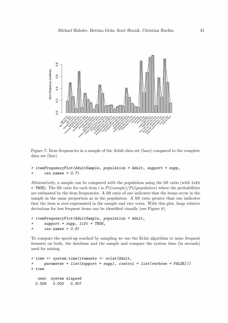
Michael Hahsler, Bettina Grun, Kurt Hornik, Christian Buchta 31
item
freq
uenc
y (r
elat
ive)
0.0
0.2
0.4
0.6
0.8
age=
Youn
g
age=
Midd
le−ag
ed
age=
Senior
workc
lass=
Loca
l−gov
workc
lass=
Privat
e
workc
lass=
Self−e
mp−
not−
inc
educ
ation
=HS−g
rad
educ
ation
=Som
e−co
llege
educ
ation
=Bac
helor
s
educ
ation
=Mas
ters
mar
ital−s
tatu
s=Divo
rced
mar
ital−s
tatu
s=M
arrie
d−civ
−spo
use
mar
ital−s
tatu
s=Nev
er−m
arrie
d
occu
patio
n=Adm
−cler
ical
occu
patio
n=Cra
ft−re
pair
occu
patio
n=Exe
c−m
anag
erial
occu
patio
n=M
achin
e−op
−insp
ct
occu
patio
n=Oth
er−s
ervic
e
occu
patio
n=Pro
f−sp
ecial
ty
occu
patio
n=Sale
s
relat
ionsh
ip=Hus
band
relat
ionsh
ip=Not
−in−f
amily
relat
ionsh
ip=Own−
child
relat
ionsh
ip=Unm
arrie
d
race
=Blac
k
race
=Whit
e
sex=
Fem
ale
sex=
Male
capit
al−ga
in=Non
e
capit
al−los
s=Non
e
hour
s−pe
r−wee
k=Par
t−tim
e
hour
s−pe
r−wee
k=Full
−tim
e
hour
s−pe
r−wee
k=Ove
r−tim
e
nativ
e−co
untry
=Unit
ed−S
tate
s
incom
e=sm
all
incom
e=lar
ge
Figure 7: Item frequencies in a sample of the Adult data set (bars) compared to the completedata set (line).
> itemFrequencyPlot(AdultSample, population = Adult, support = supp,
+ cex.names = 0.7)
Alternatively, a sample can be compared with the population using the lift ratio (with lift
= TRUE). The lift ratio for each item i is P (i|sample)/P (i|population) where the probabilitiesare estimated by the item frequencies. A lift ratio of one indicates that the items occur in thesample in the same proportion as in the population. A lift ratio greater than one indicatesthat the item is over-represented in the sample and vice versa. With this plot, large relativedeviations for less frequent items can be identified visually (see Figure 8).
> itemFrequencyPlot(AdultSample, population = Adult,
+ support = supp, lift = TRUE,
+ cex.names = 0.9)
To compare the speed-up reached by sampling we use the Eclat algorithm to mine frequentitemsets on both, the database and the sample and compare the system time (in seconds)used for mining.
> time <- system.time(itemsets <- eclat(Adult,
+ parameter = list(support = supp), control = list(verbose = FALSE)))
> time
user system elapsed
0.308 0.000 0.307

32 Introduction to arules
age=
Youn
gag
e=M
iddl
e−ag
edag
e=S
enio
rw
orkc
lass
=Lo
cal−
gov
wor
kcla
ss=
Priv
ate
wor
kcla
ss=
Sel
f−em
p−no
t−in
ced
ucat
ion=
HS
−gr
aded
ucat
ion=
Som
e−co
llege
educ
atio
n=B
ache
lors
educ
atio
n=M
aste
rsm
arita
l−st
atus
=D
ivor
ced
mar
ital−
stat
us=
Mar
ried−
civ−
spou
sem
arita
l−st
atus
=N
ever
−m
arrie
doc
cupa
tion=
Adm
−cl
eric
aloc
cupa
tion=
Cra
ft−re
pair
occu
patio
n=E
xec−
man
ager
ial
occu
patio
n=M
achi
ne−
op−
insp
ctoc
cupa
tion=
Oth
er−
serv
ice
occu
patio
n=P
rof−
spec
ialty
occu
patio
n=S
ales
rela
tions
hip=
Hus
band
rela
tions
hip=
Not
−in
−fa
mily
rela
tions
hip=
Ow
n−ch
ildre
latio
nshi
p=U
nmar
ried
race
=B
lack
race
=W
hite
sex=
Fem
ale
sex=
Mal
eca
pita
l−ga
in=
Non
eca
pita
l−lo
ss=
Non
eho
urs−
per−
wee
k=P
art−
time
hour
s−pe
r−w
eek=
Ful
l−tim
eho
urs−
per−
wee
k=O
ver−
time
nativ
e−co
untr
y=U
nite
d−S
tate
sin
com
e=sm
all
inco
me=
larg
e
lift r
atio
1.00
1.05
1.10
Figure 8: Deviations of the item frequencies in the sample from the complete Adult data set.
> timeSample <- system.time(itemsetsSample <- eclat(AdultSample,
+ parameter = list(support = supp), control = list(verbose = FALSE)))
> timeSample
user system elapsed
0.056 0.000 0.057
The first element of the vector returned by system.time() gives the (user) CPU time neededfor the execution of the statement in its argument. Therefore, mining the sample instead ofthe whole data base results in a speed-up factor of:
> # speed up
> time[1] / timeSample[1]
user.self
5.5
To evaluate the accuracy for the itemsets mined from the sample, we analyze the differencebetween the two sets.
> itemsets
set of 8496 itemsets

Michael Hahsler, Bettina Grun, Kurt Hornik, Christian Buchta 33
> itemsetsSample
set of 8427 itemsets
The two sets have roughly the same size. To check if the sets contain similar itemsets, wematch the sets and see what fraction of frequent itemsets found in the database were alsofound in the sample.
> match <- match(itemsets, itemsetsSample, nomatch = 0)
> ## remove no matches
> sum(match > 0) / length(itemsets)
[1] 0.9676318
Almost all frequent itemsets were found using the sample. The summaries of the supportof the frequent itemsets which were not found in the sample and the itemsets which werefrequent in the sample although they were infrequent in the database, respectively, give:
> summary(quality(itemsets[match == 0])$support)
Min. 1st Qu. Median Mean 3rd Qu. Max.
0.05002 0.05050 0.05110 0.05135 0.05190 0.05632
> summary(quality(itemsetsSample[-match])$support)
Min. 1st Qu. Median Mean 3rd Qu. Max.
0.05005 0.05060 0.05125 0.05155 0.05212 0.05646
This shows that only itemsets with support very close to the minimum support were falselymissed or found.
For the frequent itemsets which were found in the database and in the sample, we can calculateaccuracy from the the error rate.
> supportItemsets <- quality(itemsets[which(match > 0)])$support
> supportSample <- quality(itemsetsSample[match])$support
> accuracy <- 1 - abs(supportSample - supportItemsets) / supportItemsets
> summary(accuracy)
Min. 1st Qu. Median Mean 3rd Qu. Max.
0.8549 0.9598 0.9764 0.9721 0.9885 1.0000
The summary shows that sampling resulted in finding the support of itemsets with highaccuracy. This small example illustrates that for extremely large databases or for applicationwhere mining time is important, sampling can be a powerful technique.
34 Introduction to arules
6. Summary and outlook
With package arules we provide the basic infrastructure which enables us to mine associationsand analyze and manipulate the results. Previously, in R there was no such infrastructureavailable. The main features of arules are:
❼ Efficient implementation using sparse matrices.
❼ Simple and intuitive interface to manipulate and analyze transaction data, sets of item-sets and rules with subset selection and sorting.
❼ Interface to two fast mining algorithms.
❼ Flexibility in terms of adding new quality measures, and additional item and transac-tion descriptions which can be used for selecting transactions and analyzing resultingassociations.
❼ Extensible data structure to allow for easy implementation of new types of associationsand interfacing new algorithms.
There are several interesting possibilities to extend arules. For example, it would be veryuseful to interface algorithms which use statistical measures to find “interesting” itemsets(which are not necessarily frequent itemsets as used in an association rule context). Suchalgorithms include implementations of the χ2-test based algorithm by Silverstein, Brin, andMotwani (1998) or the baseline frequency approach by DuMouchel and Pregibon (2001). Also,the implementation of distance based clustering in arules could be used for visualization ofassociations (see e.g., Strehl and Ghosh 2003).
Acknowledgments
Part of arules was developed during the project “Statistical Computing with R” funded by ofthe “Jubilaumsstiftung der WU Wien.” The authors of arules would like to thank ChristianBorgelt for the implementation of Apriori and Eclat.
References
Aggarwal CC, Procopiuc CM, Yu PS (2002). “Finding Localized Associations in MarketBasket Data.” Knowledge and Data Engineering, 14(1), 51–62.
Agrawal R, Imielinski T, Swami A (1993). “Mining Association Rules between Sets of Itemsin Large Databases.” In Proceedings of the 1993 ACM SIGMOD International Conferenceon Management of Data, pp. 207–216. ACM Press. URL http://doi.acm.org/10.1145/
170035.170072.
Agrawal R, Srikant R (1994). “Fast Algorithms for Mining Association Rules.” In JB Bocca,M Jarke, C Zaniolo (eds.), Proc. 20th Int. Conf. Very Large Data Bases, VLDB, pp. 487–499. Morgan Kaufmann.

Michael Hahsler, Bettina Grun, Kurt Hornik, Christian Buchta 35
Asuncion A, Newman DJ (2007). UCI Repository of Machine Learning Databases. Universityof California, Irvine, Deptartment of Information and Computer Sciences. URL http:
//www.ics.uci.edu/~mlearn/MLRepository.html.
Bates D, Maechler M (2005). Matrix: A Matrix Package for R. R package version 0.95-5.
Bayardo R, Agrawal R, Gunopulos D (2000). “Constraint-based rule mining in large, densedatabases.” Data Mining and Knowledge Discovery, 4(2/3), 217–240.
Berry MJA, Linoff GS (1997). Data Mining Techniques for Marketing, Sales and CustomerSupport. Wiley Computer Publishing.
Borgelt C (2003). “Efficient Implementations of Apriori and Eclat.” In FIMI’03: Proceedingsof the IEEE ICDM Workshop on Frequent Itemset Mining Implementations.
Borgelt C (2004). Finding Association Rules/Hyperedges with the Apriori Algorithm. Work-ing Group Neural Networks and Fuzzy Systems, Otto-von-Guericke-University of Magde-burg, Universitatsplatz 2, D-39106 Magdeburg, Germany. URL http://fuzzy.cs.
uni-magdeburg.de/~borgelt/apriori.html.
Borgelt C, Kruse R (2002). “Induction of Association Rules: Apriori Implementation.” InProc. 15th Conf. on Computational Statistics (Compstat 2002, Berlin, Germany). PhysikaVerlag, Heidelberg, Germany.
Brin S, Motwani R, Ullman JD, Tsur S (1997). “Dynamic Itemset Counting and ImplicationRules for Market Basket Data.” In SIGMOD 1997, Proceedings ACM SIGMOD Interna-tional Conference on Management of Data, pp. 255–264. Tucson, Arizona, USA.
DuMouchel W, Pregibon D (2001). “Empirical Bayes Screening for Multi-Item Associations.”In F Provost, R Srikant (eds.), Proceedings of the ACM SIGKDD Intentional Conferenceon Knowledge Discovery in Databases & Data Mining (KDD01), pp. 67–76. ACM Press.
Fowler M (2004). UML Distilled: A Brief Guide to the Standard Object Modeling Language.third edition. Addison-Wesley Professional.
Goethals B, Zaki MJ (eds.) (2003). FIMI’03: Proceedings of the IEEE ICDM Workshop onFrequent Itemset Mining Implementations. Sun SITE Central Europe (CEUR).
Goethals B, Zaki MJ (2004). “Advances in Frequent Itemset Mining Implementations: Reporton FIMI’03.” SIGKDD Explorations, 6(1), 109–117.
Gupta GK, Strehl A, Ghosh J (1999). “Distance Based Clustering of Association Rules.” InProc. ANNIE 1999, St. Louis, volume 9, pp. 759–764. ASME. ISBN 0-7918-0098-9.
Hahsler M, Buchta C, Hornik K (2008). “Selective Association Rule Generation.” Computa-tional Statistics, 23(2), 303–315. ISSN ISSN 0943-4062.
Hahsler M, Grun B, Hornik K (2005a). “arules – A Computational Environment for MiningAssociation Rules and Frequent Item Sets.” Journal of Statistical Software, 14(15), 1–25.ISSN 1548-7660. URL http://www.jstatsoft.org/v14/i15/.

36 Introduction to arules
Hahsler M, Hornik K (2007a). “Building on the arules Infrastructure for Analyzing TransactionData with R.” In R Decker, HJ Lenz (eds.), Advances in Data Analysis, Proceedings of the30th Annual Conference of the Gesellschaft fur Klassifikation e.V., Freie Universitat Berlin,March 8–10, 2006, Studies in Classification, Data Analysis, and Knowledge Organization,pp. 449–456. Springer-Verlag.
Hahsler M, Hornik K (2007b). “New Probabilistic Interest Measures for Association Rules.”Intelligent Data Analysis, 11(5), 437–455. ISSN 1088-467X.
Hahsler M, Hornik K, Reutterer T (2005b). “Implications of Probabilistic Data Model-ing for Rule Mining.” Technical Report 14, Department of Statistics and Mathematics,Wirschaftsuniversitat Wien, Augasse 2-6, 1090 Wien. URL http://epub.wu-wien.ac.
at/dyn/openURL?id=oai:epub.wu-wien.ac.at:epub-wu-01_7f0.
Hastie T, Tibshirani R, Friedman J (2001). The Elements of Statistical Learning (DataMining, Inference and Prediction). Springer Verlag.
Hipp J, Guntzer U, Nakhaeizadeh G (2000). “Algorithms for Association Rule Mining – AGeneral Survey and Comparison.” SIGKDD Explorations, 2(2), 1–58.
Hofmann H, Wilhelm A (2001). “Visual comparison of association rules.” ComputationalStatistics, 16(3), 399–415. ISSN ISSN 0943-4062.
Knuth D (1997). The Art of Computer Programming, Sorting and Searching, volume 3,chapter Digital Searching, pp. 492–512. third edition.
Liu B, Hsu W, Ma Y (1999). “Pruning and summarizing the discovered associations.” InProceedings of the fifth ACM SIGKDD international conference on Knowledge discoveryand data mining (KDD-99), pp. 125–134. ACM Press.
Mannila H, Toivonen H, Verkamo AI (1994). “Efficient algorithms for discovering associationrules.” In UM Fayyad, R Uthurusamy (eds.), AAAI Workshop on Knowledge Discovery inDatabases (KDD-94), pp. 181–192. AAAI Press, Seattle, Washington.
Omiecinski ER (2003). “Alternative Interest Measures for Mining Associations in Databases.”IEEE Transactions on Knowledge and Data Engineering, 15(1), 57–69.
Parthasarathy S (2002). “Efficient Progressive Sampling for Association Rules.” In Proceedingsof the 2002 IEEE International Conference on Data Mining (ICDM’02), pp. 354–361. IEEEComputer Society.
Pasquier N, Bastide Y, Taouil R, Lakhal L (1999). “Discovering Frequent Closed Itemsets forAssociation Rules.” In Proceeding of the 7th International Conference on Database Theory,Lecture Notes In Computer Science (LNCS 1540), pp. 398–416. Springer.
Piatetsky-Shapiro G (1991). “Discovery, Analysis, and Presentation of Strong Rules.” InG Piatetsky-Shapiro, WJ Frawley (eds.), Knowledge Discovery in Databases. AAAI/MITPress, Cambridge, MA.
R Development Core Team (2005). R: A Language and Environment for Statistical Comput-ing. R Foundation for Statistical Computing, Vienna, Austria. ISBN 3-900051-07-0, URLhttp://www.R-project.org.

Michael Hahsler, Bettina Grun, Kurt Hornik, Christian Buchta 37
Silverstein C, Brin S, Motwani R (1998). “Beyond Market Baskets: Generalizing AssociationRules to Dependence Rules.” Data Mining and Knowledge Discovery, 2, 39–68.
Srikant R, Agrawal R (1996). “Mining Quantitative Association Rules in Large RelationalTables.” In HV Jagadish, IS Mumick (eds.), Int. Conf. on Management of Data, SIGMOD,pp. 1–12. ACM Press.
Strehl A, Ghosh J (2003). “Relationship-Based Clustering and Visualization for High-Dimensional Data Mining.” INFORMS Journal on Computing, 15(2), 208–230.
Tan PN, Kumar V, Srivastava J (2004). “Selecting the right objective measure for associationanalysis.” Information Systems, 29(4), 293–313.
Toivonen H (1996). “Sampling Large Databases for Association Rules.” In Proceedings of the22th International Conference on Very Large Data Bases, pp. 134–145. Morgan KaufmannPublishers Inc.
Williams G (2008). pmml: Generate PMML for various models. R package version 1.1.7.
Xiong H, Tan PN, Kumar V (2003). “Mining Strong Affinity Association Patterns in DataSets with Skewed Support Distribution.” In B Goethals, MJ Zaki (eds.), Proceedings ofthe IEEE International Conference on Data Mining, November 19–22, 2003, Melbourne,Florida, pp. 387–394.
Zaki MJ (2000). “Scalable Algorithms for Association Mining.” IEEE Transactions on Knowl-edge and Data Engineering, 12(3), 372–390.
Zaki MJ (2004). “Mining Non-Redundant Association Rules.” Data Mining and KnowledgeDiscovery, 9, 223–248.
Zaki MJ, Parthasarathy S, Li W, Ogihara M (1997a). “Evaluation of Sampling for Data Miningof Association Rules.” In Proceedings of the 7th International Workshop on Research Issuesin Data Engineering (RIDE ’97) High Performance Database Management for Large-ScaleApplications, pp. 42–50. IEEE Computer Society.
Zaki MJ, Parthasarathy S, Ogihara M, Li W (1997b). “New Algorithms for Fast Discoveryof Association Rules.” Technical Report 651, Computer Science Department, University ofRochester, Rochester, NY 14627.
Affiliation:
Michael HahslerEngineering Management, Information, and SystemsLyle School of EngineeringSouthern Methodist UniversityP.O. Box 750122Dallas, TX 75275-0122E-mail: [email protected]: http://lyle.smu.edu/~mhahsler